Estimating the cluster tree of a density byanalyzing the minimal spanning tree of a

sample

Werner Stuetzle ∗

Department of StatisticsUniversity of Washington

wxs@stat.washington.edu

February 12, 2003

Abstract

We present runt pruning, a new clustering method that attemptsto find modes of a density by analyzing the minimal spanning tree ofa sample. The method exploits the connection between the minimalspanning tree and nearest neighbor density estimation. It does notrely on assumptions about the specific form of the data density (e.g.,normal mixture) or about the geometric shapes of the clusters, and iscomputationally feasible for large data sets.

Keywords: Two-way, two-mode data; nearest neighbor density esti-mation; single linkage clustering; runt test; mixture models.

∗Supported by NSF grant DMS-9803226 and NSA grant 62-1942. Work partially per-formed while on sabbatical at AT&T Labs - Research. Author’s address: Department ofStatistics, Box 354322, University of Washington, Seattle, WA 98195-4322; email: wxs-stat.washington.edu

1

1 Introduction

The goal of clustering is to identify distinct groups in a two-mode, two-waydataset X = {x1, . . . ,xn} ⊂ Rm. For example, when presented with (atypically higher dimensional version of) a data set like the one in Figure 1we would like to detect that there appear to be (perhaps) five or six distinctgroups, and assign a group label to each observation.

Figure 1: Data set with 5–6 apparent groups.

To cast clustering as a statistical problem we regard the data x1, . . . ,xn

as an iid sample form some unknown probability density p(x). There aretwo statistical approaches to clustering. The parametric approach (Fraleyand Raftery 1998, 1999; McLachlan and Peel 2000) is based on the assump-tion that each group g is represented by a density pg(x) that is a memberof some parametric family, such as the multivariate Gaussian distributions.The density p(x) then is a mixture of the group densities, and the numberof mixture components and their parameters are estimated from the data.Observations can be labeled using Bayes’s rule.

In contrast, the nonparametric approach adopted in this paper is basedon the premise that groups correspond to modes of the density p(x). The

2

goal then is to find the modes and assign each observation to the “domainof attraction” of a mode. Searching for modes as a manifestation of thepresence of groups was first advocated in D. Wishart’s (1969) paper on ModeAnalysis. According to Wishart, clustering methods should be able to detectand “resolve distinct data modes, independently of their shape and variance”.

Hartigan (1975, Section 11; 1981) expanded on Wishart’s idea and madeit more precise by introducing the notion of high density clusters. Define thelevel set L(λ; p) of a density p at level λ as the subset of the feature spacefor which the density exceeds λ:

L(λ; p) = {x | p(x) > λ}.The high density clusters at level λ are the maximally connected subsets ofL(λ; p).

Hartigan also pointed out that the collection of high density clusters hasa hierarchical structure: for any two clusters A and B (possibly at differentlevels) we have either A ⊂ B or B ⊂ A or A ∩ B = ∅. This hierarchicalstructure is summarized by the cluster tree of p. Each node N of the treerepresents a subset D(N) of the support L(0; p) of p — a high density clusterof p — and is associated with a density level λ(N). The cluster tree is easiestto define recursively. The root node represents the entire support of p, andhas associated density level λ(N) = 0. To determine the descendents of anode N we find the lowest level λd for which L(λ; p) ∩ D(N) has two ormore connected components. If there is no such λd then p has only onemode in D(N), and N is a leaf of the tree. Otherwise, let C1, . . . , Ck be theconnected components of L(λd; p)∩D(N). If k = 2 (the usual case) we createdaughter nodes representing the connected components C1 and C2, both withassociated level λd, and apply the definition recursively to the daughters. Ifk > 2 we create daughter nodes representing C1 and C2∪· · ·∪Ck and recurse.

Figure 2 shows a density and the corresponding cluster tree. Estimatingthe cluster tree is a fundamental goal of nonparametric cluster analysis.

1.1 Previous work

Several previously suggested clustering methods can be described in termsof levels sets and high density clusters.

Probably the earliest such method is Wishart’s (1969) one level modeanalysis. The goal of one level mode analysis is to find the high density clus-

3

Figure 2: Density and corresponding tree of high density clusters.

ters at a given density level λ chosen by the user. The idea is to first computea kernel density estimate p (Silverman 1986, Chapter 4) and set aside all ob-servations with p(xi) ≤ λ, i.e., all observations not in the level set L(λ; p).If the population density has several well separated high density clusters atlevel λ then the remaining high density observations should fall into clearlyseparated groups. Wishart suggests using single linkage clustering of thehigh density observations to identify the groups. One level mode analysisanticipates some of the “sharpening” ideas later put forth by P.A. Tukeyand J.W. Tukey (1981).

A reincarnation of one level mode analysis is the DBScan algorithm ofEster, Kriegel, Sander, and Xu (1996). DBScan consists of four steps: (a)for each data point calculate a kernel density estimate using a sphericaluniform kernel with radius r; (b) choose a density threshold λ and findthe observations with p(xi) > λ; (c) construct a graph connecting each highdensity observation to all other observations within distance r; (d) define theclusters to be the connected components of this graph. All observations notwithin distance r of a high density observation are considered “noise”.

A weakness of one level mode analysis is apparent from Figure 2. The

4

degree of separation between connected components of L(λ; p), and thereforeof L(λ; p), depends critically on the choice of the cut level λ, which is left tothe user. Moreover, there might not be a single value of λ that reveals allthe modes.

Citing the difficulty in choosing a cut level, Wishart (1969) proposed hi-erarchical mode analysis, which can be regarded as a heuristic for comput-ing the cluster tree of a kernel density estimate p, although it appears thatWishart did not view it thus. (The word “tree” does not occur in the sectionof his paper on hierarchical mode analysis.) We use the term “heuristic”because there is no guarantee that hierarchical mode analysis will indeedcorrectly compute the cluster tree of p as defined above. Wishart’s (1969)algorithm constructs the tree by iterative merging (i.e., is an agglomerativealgorithm). It is quite complex, probably because its iterative approach isnot well matched to the tree structure it is trying to generate.

The basic weakness of one level mode analysis was also noted by Ankerst,Breuning, Kriegel, and Sander (1999) who proposed OPTICS, an algorithmfor “Ordering Points to Identify the Clustering Structure”. OPTICS gen-erates a data structure that allows one to calculate efficiently the result ofDBScan for any desired density threshold λ. It also produces a graphicalsummary of the cluster structure. The idea behind their algorithm is hardto understand.

1.2 Outline of runt pruning

An obvious way of estimating the cluster tree of a density p from a sampleis to first compute a density estimate p and then use the cluster tree of p asan estimate for the cluster tree of p. A difficulty with this approach is thatfor most density estimates computing the cluster tree seems computationallyintractable. To determine the number of connected components of a levelset L(λ; p) one would have to rely on heuristics, like the ones suggested byWishart (1969) and Ester et al. (1996), which is at the very least an estheticdrawback. A notable exception is the nearest neighbor density estimate

p1(y) =1

n V d(y,X )p,

where V is the volume of the unit sphere in Rm and d(y,X ) = mini d(y,xi).In Section 2 we show that the cluster tree of the nearest neighbor density

5

estimate is isomorphic to the single linkage dendogram. The argument ex-ploits a connection between the minimal spanning tree (MST) and nearestneighbor density estimation first pointed out by Hartigan (1985).

The nearest neighbor density estimate has some undesirable properties.For example, it has a high variance and it cannot be normalized. As weare not interested in estimating the density itself but rather its cluster tree,these flaws are not necessarily fatal. However, it also has a singularity atevery data point, leading to a cluster tree with as many leaves as there areobservations. Therefore the cluster tree has to be pruned.

Our pruning method, runt pruning, is based on the runt test for multi-modality proposed by Hartigan and Mohanty (1992). In Section 3 we describerunt pruning, provide a heuristic justification for the method, and presentan algorithm.

In Section 4 we compare runt pruning to the standard single linkagemethod for extracting clusters from a MST. In Section 5 we show runt prun-ing in action, illustrate diagnostic tools that can be helpful in choosing therunt size threshold determining tree size, and compare its performance toother clustering methods. In Section 6 we discuss some general issues suchas the underlying assumptions and the relative merits of parametric andnonparametric clustering methods. Section 7 concludes the paper with asummary and ideas for future work.

2 Nearest neighbor density estimation and

the Euclidean minimal spanning tree

In this section we show that the cluster tree of the nearest neighbor densityestimate can be obtained from the MST of the data, and that it is isomorphicto the single linkage dendogram. For a given density level λ, define

r(λ) =(

1

n V λ

) 1p

.

By definition, p1(y) > λ iff d(y,X ) < r(λ), and therefore L(λ; p1) is theunion of (open) spheres of radius r(λ), centered at the observations:

L(λ; p1) =⋃i

◦S (xi, r(λ)) .

6

Let T be the Euclidean MST of X , that is, the graph with shortest totaledge length connecting all the observations. Breaking all MST edges withlength ≥ 2r(λ) defines a partition of the MST into k subtrees T1, . . . , Tk (pos-sible k = 1) and a corresponding partition of the observations into subsetsX1, . . . ,Xk.

Proposition 1: (Hartigan 1985): The sets Li =⋃

i∈Xj

◦S (xi, r(λ)) are

the connected components of L(λ; p1).

Proof: Each of the sets Li is connected, because by construction themaximum edge length of the corresponding MST fragment Ti is smaller than2r(λ), and therefore the MST fragment is a subset of Li.

On the other hand, Li and Lj are disconnected for i �= j. Otherwise therewould have to be observations x∗ and x∗∗ in Xi and Xj , respectively, withd(x∗,x∗∗) < 2r(λ). We could then break an edge of length ≥ 2r(λ) in theMST path connecting fragments Ti and Tj and insert an edge connecting x∗

and x∗∗, thereby obtaining a spanning tree of smaller total edge length. Thiscontradicts the assumption that T was the MST.

Proposition 1 implies that we can compute the cluster tree of the nearestneighbor density estimate by breaking the longest edge of the MST, therebysplitting the MST into two subtrees, and then applying the splitting oper-ation recursively to the subtrees. Gower and Ross (1969) show that thisalgorithm finds the single linkage dendogram, which demonstrates that thecluster tree of the nearest neighbor density estimate and the single linkagedendogram are isomorphic.

3 Runt pruning

The nearest neighbor density estimate has a singularity at every observation,and consequently its cluster tree — the single linkage dendogram — has asmany leaves as there are observations and is a poor estimate for the clustertree of the underlying density. It has to be pruned.

Runt pruning is based on the runt test for multimodality proposed byHartigan and Mohanty (1992). They define the runt size of a dendogramnode N as the smaller of the number of leaves of the two subtrees rootedat N . If we interpret the single linkage dendogram as the cluster tree of

7

the nearest neighbor density estimate p1, then a node N and its daughtersrepresent high density clusters of p1. The runt size of N can therefore alsobe regarded as the smaller of the number of observations falling into the twodaughter clusters. As each node of the single linkage dendogram correspondsto an edge of the MST, we can also define the runt size for an MST edge e:Break all MST edges that are as long or longer than e. The two MST nodesoriginally joined by e are the roots of two subtrees of the MST, and the runtsize of e is the smaller of the number of nodes of those subtrees.

The idea of runt pruning is to consider a split of a high density clusterof p1 into two connected components to be “real” or “significant” if bothdaughters contain a sufficiently large number of observations, i.e., if the runtsize of the corresponding dendogram node is larger than some threshold. Therunt size threshold controls the size of the estimated cluster tree.

3.1 Heuristic justification

MST edges with large runt size indicate the presence of multiple modes,as was first observed by Hartigan and Mohanty (1992). We can verify thisassertion by considering a simple algorithm for computing a MST: Definethe distance between two groups of observations G1 and G2 as the minimumdistance between observations:

d(G1, G2) = minx∈G1

miny∈G2

d(x,y) .

Initialize each observation to form its own group. Find the two closest groups,add the shortest edge connecting them to the graph, and merge the twogroups. Repeat this merge step until only one group remains. The runt sizeof an edge is the size of the smaller of the two groups connected by the edge.

Suppose now that the underlying density is multimodal. Initial mergestend to take place in high density regions where interpoint distances aresmall, and tree fragments will tend to grow in those regions. Eventually,those fragments will have to be joined by edges, and those edges will havelarge runt sizes, as illustrated in Figure 3. Panel (a) shows a sample from abimodal density, and panel (b) shows the corresponding rootogram of runtsizes. (A rootogram is a version of a histogram where the square roots ofthe counts are plotted on the vertical axis.) There is one edge with runt size75. Panel (c) shows the MST after removal of all edges with length greater

8

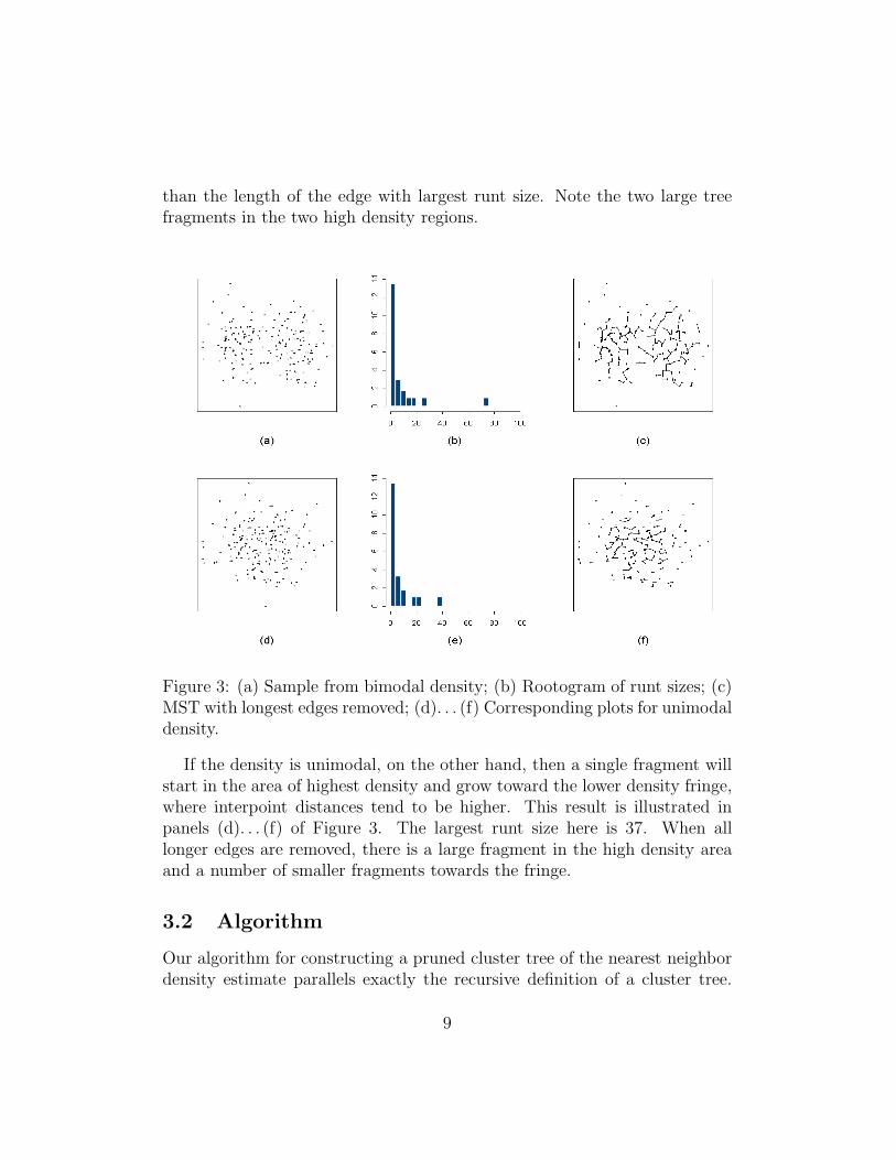
than the length of the edge with largest runt size. Note the two large treefragments in the two high density regions.

Figure 3: (a) Sample from bimodal density; (b) Rootogram of runt sizes; (c)MST with longest edges removed; (d). . . (f) Corresponding plots for unimodaldensity.

If the density is unimodal, on the other hand, then a single fragment willstart in the area of highest density and grow toward the lower density fringe,where interpoint distances tend to be higher. This result is illustrated inpanels (d). . . (f) of Figure 3. The largest runt size here is 37. When alllonger edges are removed, there is a large fragment in the high density areaand a number of smaller fragments towards the fringe.

3.2 Algorithm

Our algorithm for constructing a pruned cluster tree of the nearest neighbordensity estimate parallels exactly the recursive definition of a cluster tree.

9

Each node N represents a high density cluster D(N) of p1, a sample clustercore X (N) consisting of the observations in D(N), and a subtree T (N) of theMST, and is associated with a density level λ(N). The root node representsthe entire feature space, sample, and MST, and is associated with densitylevel λ = 0.

To determine the descendents of a node N we find the lowest density levelλ or, equivalently, the longest edge e in T (N) with runt size larger than ourchosen threshold. If there is no such edge then N is a leaf of the tree.

Otherwise, we create daughter nodes Nr and Nl associated with densitylevel

λ(Nl) = λ(Nr) =2m

nV ‖e‖m.

Breaking all edges of T (N) with length ≥ ‖e‖ results in a subgraph of T (N);the sample cluster cores X (Nl) and X (Nr) consist of the observations in thefragments rooted at the ends of e. The high density clusters D(Nl) andD(Nr) are unions of spheres of radius ‖e‖/2 centered at the observations inX (Nl) and X (Nr), respectively. The trees T (Nl) and T (Nr) are obtained bybreaking the edge e of T (N).

We refer to the observations in T (N) as the sample cluster or, if there isno ambiguity, simply as the cluster represented by N . If N1, . . . , Nk are theleaves of the cluster tree, then the corresponding clusters form a partition ofthe sample. The cluster cores X (Ni) are subsets of the corresponding clusterslocated in the high density regions.

4 Runt pruning and single linkage clustering

The standard method for extracting clusters from a MST is single linkageclustering: to create k clusters, break the k − 1 longest edges in the MST.This approach can be successful if the groups are clearly separated, i.e.,if the Hausdorff distance between groups is large compared to the typicalnearest neighbor distance. For an illustration, see the “Bullseye”” example inSection 5.2. However, in situations where the grouping is not quite as obvious,single linkage clustering tends to fail, and it has acquired a (deservedly) badreputation. There are two reasons for this failure.

First, single linkage clustering tends to generate many small clusters be-cause the longest edges of the minimal spanning tree will be in low density

10

regions, which typically are at the periphery of the data: long edges tend toconnect stragglers to the bulk.

Second, choosing a single edge length threshold for defining clusters isequivalent to looking at a single level set of the nearest neighbor densityestimate. However, as Figure 2 illustrates, there are densities where no singlelevel set will reveal all the modes. Therefore single linkage clustering cannotbe “repaired” by simply discarding all small clusters and considering onlythe large ones as significant — the problem is more fundamental.

5 Examples

We present four examples. The first, simulated data with highly nonlinearcluster shapes, demonstrates that runt analysis can indeed find such structurefor which other algorithms, like average linkage, complete linkage, and model-based clustering fail.

The second example, simulated data with spherical Gaussian clusters, isdesigned to be most favorable for model-based clustering and suggests thatthe performance penalty of runt pruning in such cases is not disastrous.

The third example, data on the chemical compositions of 572 olive oilsamples from nine different areas of Italy, is used to illustrate how we mightset a runt size threshold, and how we can use diagnostic plots to assesswhether clusters are real or spurious.

The fourth example, 256-dimensional data encoding the shapes of hand-written digits, shows that runt pruning can be reasonably applied to high-dimensional data, despite the fact that it is based on a poor density estimate.

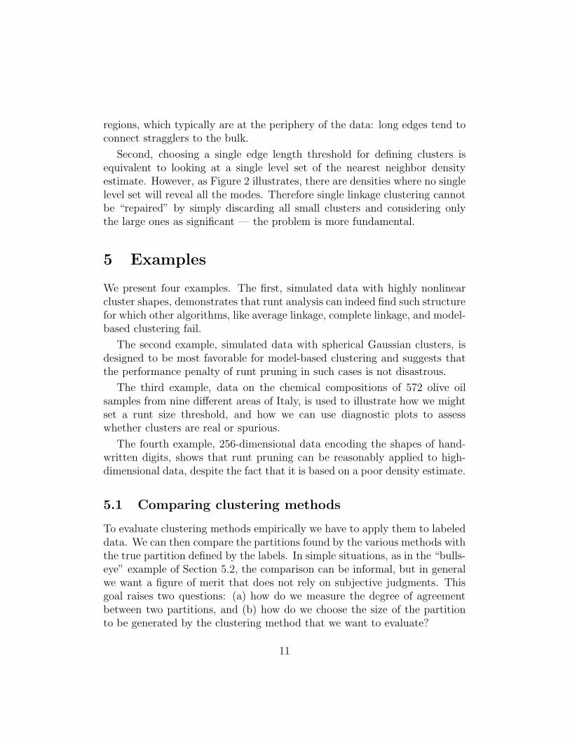
5.1 Comparing clustering methods

To evaluate clustering methods empirically we have to apply them to labeleddata. We can then compare the partitions found by the various methods withthe true partition defined by the labels. In simple situations, as in the “bulls-eye” example of Section 5.2, the comparison can be informal, but in generalwe want a figure of merit that does not rely on subjective judgments. Thisgoal raises two questions: (a) how do we measure the degree of agreementbetween two partitions, and (b) how do we choose the size of the partitionto be generated by the clustering method that we want to evaluate?

11

Measuring agreement between partitions. Let P1 and P2 be twopartitions of a set of n objects. The partitions define a contingency table:let nij be the number of objects that belong to subset i of partition P1 andto subset j of partition P2. We measure the agreement between P1 and P2

by the adjusted Rand index (Hubert and Arabie 1985) defined as

R =

∑ij

(nij

2

)− ∑

i

(ni·2

) ∑j

(n·j2

)/(

n2

)12

(∑i

(ni·2

)+

∑j

(n·j2

))− ∑

i

(ni·2

) ∑j

(n·j2

)/(

n2

) .

Here ni· =∑

j nij , and n·j is defined analogously.

The adjusted Rand index has a maximum value of 1 which is achievedwhen the two partitions are identical up to re-numbering of the subsets. Ithas expected value 0 under random assignment of the objects to the subsetsof P1 and P2 that leave the marginals ni· and n·j fixed.

Choosing a partition size. Choosing a partition size is a difficult issue,especially for nonparametric clustering methods, for which there is as yetno automatic method, and subjective judgment is required. To eliminatethe subjective element from the comparisons, we decompose the clusteringproblem into two subproblems: (a) determining the number of groups, and(b) finding the groups, given their number. We compare the performance onsubproblem (b), using two different rules for setting the number of groups.First, we have each method produce the true number of groups. Second, wegenerate a range of partitions of different sizes, calculate the adjusted Randindex for each of them, and then report the maximum value of the indexachieved by the method and the corresponding partition size.

5.2 Nonlinear clusters — Bullseye

The data used in this example are shown in Figure 4(a). There are 500observations uniformly distributed over the center of the bullseye and thering. Figure 4(b) shows the 2-partition generated by runt pruning of theMST. Figures 4(c),. . . , 4(e) show the 2-partitions generated by single, av-erage, and complete linkage, respectively. Figure 4(f) shows the 2-partitiongenerated by fitting Gaussian mixtures. We used the software described inFraley and Raftery (1999). The Gaussians were constrained to have equalspherical covariance matrices.

12

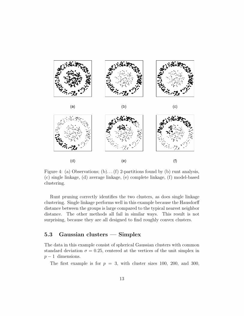
Figure 4: (a) Observations; (b). . . (f) 2-partitions found by (b) runt analysis,(c) single linkage, (d) average linkage, (e) complete linkage, (f) model-basedclustering.

Runt pruning correctly identifies the two clusters, as does single linkageclustering. Single linkage performs well in this example because the Hausdorffdistance between the groups is large compared to the typical nearest neighbordistance. The other methods all fail in similar ways. This result is notsurprising, because they are all designed to find roughly convex clusters.

5.3 Gaussian clusters — Simplex

The data in this example consist of spherical Gaussian clusters with commonstandard deviation σ = 0.25, centered at the vertices of the unit simplex inp − 1 dimensions.

The first example is for p = 3, with cluster sizes 100, 200, and 300,

13

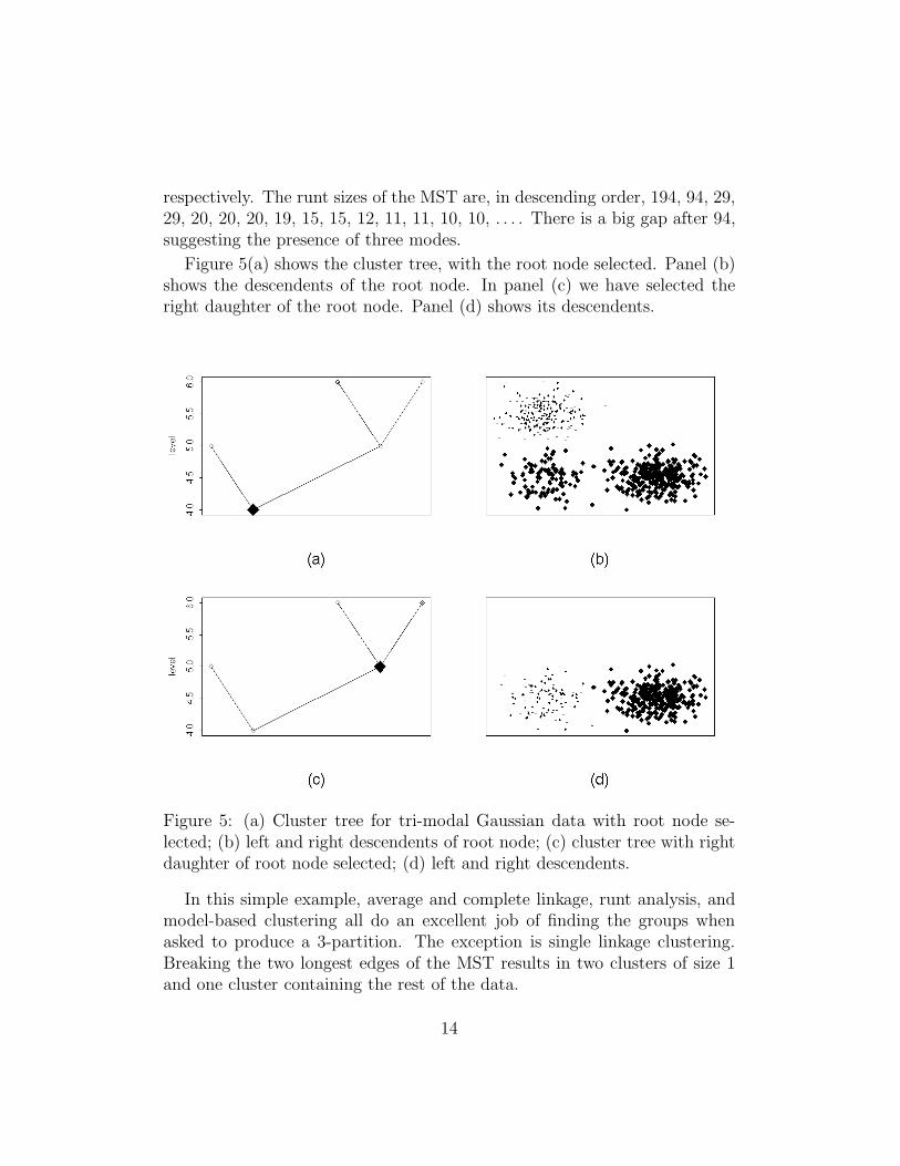
respectively. The runt sizes of the MST are, in descending order, 194, 94, 29,29, 20, 20, 20, 19, 15, 15, 12, 11, 11, 10, 10, . . . . There is a big gap after 94,suggesting the presence of three modes.

Figure 5(a) shows the cluster tree, with the root node selected. Panel (b)shows the descendents of the root node. In panel (c) we have selected theright daughter of the root node. Panel (d) shows its descendents.

Figure 5: (a) Cluster tree for tri-modal Gaussian data with root node se-lected; (b) left and right descendents of root node; (c) cluster tree with rightdaughter of root node selected; (d) left and right descendents.

In this simple example, average and complete linkage, runt analysis, andmodel-based clustering all do an excellent job of finding the groups whenasked to produce a 3-partition. The exception is single linkage clustering.Breaking the two longest edges of the MST results in two clusters of size 1and one cluster containing the rest of the data.

14

SL AL CL RP MC-EI MC-VI0.0 (0.03) 0.92 (0.01) 0.92 (0.04) 0.82 (0.05) 0.93 (0.02) 0.92 (0.01)0.0 (0.08) 0.92 (0.01) 0.92 (0.02) 0.90 (0.03) 0.93 (0.02) 0.92 (0.01)

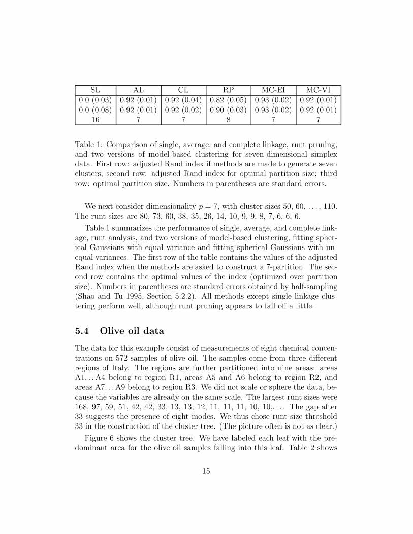
16 7 7 8 7 7

Table 1: Comparison of single, average, and complete linkage, runt pruning,and two versions of model-based clustering for seven-dimensional simplexdata. First row: adjusted Rand index if methods are made to generate sevenclusters; second row: adjusted Rand index for optimal partition size; thirdrow: optimal partition size. Numbers in parentheses are standard errors.

We next consider dimensionality p = 7, with cluster sizes 50, 60, . . . , 110.The runt sizes are 80, 73, 60, 38, 35, 26, 14, 10, 9, 9, 8, 7, 6, 6, 6.

Table 1 summarizes the performance of single, average, and complete link-age, runt analysis, and two versions of model-based clustering, fitting spher-ical Gaussians with equal variance and fitting spherical Gaussians with un-equal variances. The first row of the table contains the values of the adjustedRand index when the methods are asked to construct a 7-partition. The sec-ond row contains the optimal values of the index (optimized over partitionsize). Numbers in parentheses are standard errors obtained by half-sampling(Shao and Tu 1995, Section 5.2.2). All methods except single linkage clus-tering perform well, although runt pruning appears to fall off a little.

5.4 Olive oil data

The data for this example consist of measurements of eight chemical concen-trations on 572 samples of olive oil. The samples come from three differentregions of Italy. The regions are further partitioned into nine areas: areasA1. . . A4 belong to region R1, areas A5 and A6 belong to region R2, andareas A7. . . A9 belong to region R3. We did not scale or sphere the data, be-cause the variables are already on the same scale. The largest runt sizes were168, 97, 59, 51, 42, 42, 33, 13, 13, 12, 11, 11, 11, 10, 10,. . . . The gap after33 suggests the presence of eight modes. We thus chose runt size threshold33 in the construction of the cluster tree. (The picture often is not as clear.)

Figure 6 shows the cluster tree. We have labeled each leaf with the pre-dominant area for the olive oil samples falling into this leaf. Table 2 shows

15

Figure 6: Cluster tree for olive oil data. Nodes have been labeled withpredominant area.

the distribution of areas over clusters. Table 3 summarizes the performanceof clustering methods for the olive oil date. Runt pruning with threshold 33(eight clusters) gives an adjusted Rand index of 0.57. Again, single linkageis the lone outlier.

The split represented by the root node separates region R3 from regionsR1 and R2. The left daughter separates region R1 from region R2. Themethod erroneously splits area A3 into two clusters and was not successfulin identifying areas A1 and A4. This raises two questions: (a) do the oliveoils from area A3 really have a bimodal density, and (b) does the densityreally have modes corresponding to areas A1 and A4?

The first question is at least partly answered by Figure 7. Panel (a) showsthe cluster tree. We have selected the node N that has partitioned area A3.Panel (b) shows a rootogram (histogram with the roots of the cell countsplotted on the vertical axis) of the cluster represented by N , projected ontothe Fisher discriminant direction calculated to separate the daughter clusters.(The idea for this diagnostic plot comes from Gnanadesikan, Kettenring, andLandwehr (1982). The Fisher discriminant direction maximizes the ratioof between-cluster variance to within-cluster variance of the projected data(Mardia, Kent, and Bibby 1979, Section 11.5). In that sense it is the direction

16

1 2 3 4 5 6 7 8A1 0 1 0 0 0 17 0 7A2 0 51 1 0 0 4 0 0A3 90 11 103 1 0 0 1 0A4 5 13 4 0 0 14 0 0A5 0 0 0 64 1 0 0 0A6 0 0 0 0 33 0 0 0A7 0 3 0 0 0 43 0 4A8 0 2 0 0 0 2 45 1A9 0 0 0 0 0 0 0 51

Table 2: Olive oil data: cluster number (horizontal axis) tabulated againstarea (vertical axis).

that best reveals separation between clusters.) The rootogram does not lookbimodal. While this does not conclusively show that there is only one mode— there might be two modal regions with nonlinear shapes, so that theseparation does not manifest itself in the projection — it is an indication,and we might want to prune the tree by removing the daughters. In contrast,the rootogram in panel (d) where we have selected the node separating areaA2 from area A3, shows clear bimodality. Note that this diagnostic can beused in practical problems because it does not require knowing the true labelsof the observations.

To answer the question whether areas A1 and A4 really are separated fromareas A2 and A3 and correspond to modes of the density, we project theobservations from the four areas onto the first two discriminant coordinates(Mardia, Kent, and Bibby 1979, Section 12.5). Figure 8 shows that whileareas A2 (open circle) and A3 (filled circle) form fairly obvious groups, thisis not true for areas A1 (triangle) and A4 (cross). Again, finding this is notstrictly conclusive because we are seeing only a two-dimensional projectionof the eight-dimensional data but it is a good indication. Note that thisapproach is not an “operational” diagnostic, because in practice the truelabels of the observations would be unknown. We use it here merely to helpevaluate the performance of our method.

17

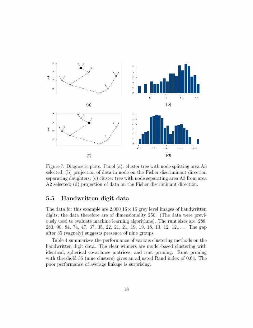
Figure 7: Diagnostic plots. Panel (a): cluster tree with node splitting area A3selected; (b) projection of data in node on the Fisher discriminant directionseparating daughters; (c) cluster tree with node separating area A3 from areaA2 selected; (d) projection of data on the Fisher discriminant direction.

5.5 Handwritten digit data

The data for this example are 2,000 16×16 grey level images of handwrittendigits; the data therefore are of dimensionality 256. (The data were previ-ously used to evaluate machine learning algorithms). The runt sizes are 288,283, 90, 84, 74, 47, 37, 35, 22, 21, 21, 19, 19, 18, 13, 12, 12,. . . . The gapafter 35 (vaguely) suggests presence of nine groups.

Table 4 summarizes the performance of various clustering methods on thehandwritten digit data. The clear winners are model-based clustering withidentical, spherical covariance matrices, and runt pruning. Runt pruningwith threshold 35 (nine clusters) gives an adjusted Rand index of 0.64. Thepoor performance of average linkage is surprising.

18

Figure 8: Projection of areas A1 (triangle), A2 (open circle), A3 (filled circle),and A4 (cross) on the plane spanned by first two discriminant coordinates.

6 Remarks

We address three issues: (a) relationship between parametric and nonpara-metric clustering; (b) distinction between clustering and compact partition-ing; (c) non-modal groups.

6.1 Parametric versus nonparametric clustering

The most appealing feature of parametric or model-based clustering is that itseems to offer a way of estimating the number of groups: Fit a mixture model

19

SL AL CL RP MC-EI MC-VI0.0 (0.03) 0.61 (0.07) 0.43 (0.04) 0.50 (0.06) 0.45 (0.04) 0.37 (0.04)0.0 (0.1) 0.64 (0.05) 0.50 (0.04) 0.70 (0.06) 0.58 (0.05) 0.61 (0.05)

15 12 7 5 8 5

Table 3: Comparison of single, average, and complete linkage, runt pruning,and two versions of model-based clustering for the olive oil data. First row:adjusted Rand index if methods are made to generate nine clusters; secondrow: adjusted Rand index for optimal partition size; third row: optimalpartition size. Numbers in parentheses are standard errors.

SL AL CL RP MC-EI MC-VI0.0 (0.0) 0.07 (0.05) 0.28 (0.05) 0.58 (0.04) 0.62 (0.03) 0.33 (0.04)0.0 (0.0) 0.29 (0.04) 0.36 (0.03) 0.69 (0.04) 0.63 (0.03) 0.36 (0.03)

20 20 19 7 15 8

Table 4: Comparison of single, average, and complete linkage, runt analysis,and two versions of model-based clustering for the handwritten digit data.First row: adjusted Rand index if methods are made to generate ten clus-ters; second row: adjusted Rand index for optimal partition size; third row:optimal partition size. Numbers in parentheses are standard errors.

to the sample and use a criterion such as BIC (Schwartz 1978) to estimatethe number of mixture components, which is then taken as an estimate forthe number of groups (Fraley and Raftery 1998). The conceptual problemwith this approach is that the optimal number of mixture components is notan intrinsic property of the data density but instead depends on the familyof distributions that are being mixed. Fitting a mixture of uniforms, or amixture of spherical Gaussians, or a mixture of general Gaussians will resultin different estimates for the number of groups. Thus, the estimated numberof groups depends on assumptions about the group distributions that aresomewhat arbitrary and unverifiable, but can sometimes be gleaned fromplots of the data.

Nonparametric clustering is based on the premise that groups correspondto modes of the density. While this assumption can also be questioned — seeSection 6.3 — at least the number of modes is an intrinsic property of the

20

density. Model-based clustering can be used in an attempt to find modes andestimate their number. A weakness of this approach is that mixture modelingestimates the number of components in a mixture, which in general will bedifferent from the number of modes.

6.2 Clustering versus compact partitioning.

It is important to distinguish between clustering and compact partitioningor dissection. The goal of compact partitioning is to split a set of objectsinto groups that are spatially compact. The degree of compactness can forexample be measured by the total squared distance between the observationsand their closest group mean vectors, the figure of merit that is optimized bythe k-means or Lloyd algorithm (MacQueen 1967). There are applications,such as vector quantization, where compact partitioning of the data makesperfect sense, even when there are no distinct groups at all. Some clusteringalgorithms, like complete linkage, are really better regarded as tools for com-pact partitioning. Compact partitioning algorithms might identify groups ifthey happen to be roughly spherical and well separated, but they will fail ifthis is not the case, as illustrated in Section 5.2.

6.3 Non-modal groups

We have assumed thus far that groups correspond to modes of the density,but this assumption may not hold. Most observers would agree that the datasets shown in Figure 9 each consist of two groups. However, these groups donot manifest themselves as modes. We are not aware of a general, automaticsolution to this problem. There appear to be two approaches.

The first is to abandon the requirement that the method be automatic.Instead we graphically present the data to an observer and rely on the humancognitive ability for detecting groups. A large collection of tools has beendeveloped for this purpose, ranging from mapping techniques like projectionpursuit (Friedman and Tukey 1974; Friedman, Stuetzle, and Schroeder 1984;Friedman 1987) to systems like XGobi (Swayne, Cook, and Buja 1998) thatare based on high interaction motion graphics.

The second approach is to transform the data such that in the transformeddata grouping manifests itself as multimodality. The prototypical example

21

for this approach is the Hough transform in computer vision (Ballard andBrown 1982, Section 4.3).

Figure 9: Groups that do not correspond to modes.

7 Summary and future work

We presented runt pruning, a new clustering method that attempts to findmodes of a density by analyzing the MST of a sample. The method exploitsthe connection between the MST and nearest neighbor density estimation. Itdoes not rely on assumptions about the specific form of the data density or thegeometric shapes of the clusters. Our (admittedly very limited) experimentssuggest that the price in performance paid for this generality is small.

There are a number of areas for future work. Probably the most importantand most difficult problem in nonparametric clustering is determining thecorrect size of the cluster tree, i.e., estimating the number of modes. Even thesimpler problem of testing for unimodality has not found a fully satisfactorysolution in the multivariate case. Existing methods, such as the dip test(Hartigan and Hartigan 1985), the runt test (Hartigan and Mohanty 1992),and the map test (Rozal and Hartigan 1994), strictly speaking, test the

22

hypotheses that the data are multivariate Gaussian or uniform, using a teststatistic that is sensitive against multimodal alternatives.

Absent an automatic solution to the problem of estimating the size of acluster tree, we have to rely on diagnostic tools that require human interac-tion. The diagnostic plots shown in Section 5 only work if the clusters canbe linearly separated. If the clusters are highly nonlinear, as in the exampleof Section 5.2, projection of the data on the Fisher discriminant directionmight not show a clear bimodality, and more powerful methods are needed.

A weakness of runt pruning is its reliance on the nearest neighbor densityestimate. One would like to use better density estimates such as k-th nearestneighbor or (adaptive) kernel estimates (see, for example, Silverman 1986,Section 2), or a Projection Pursuit estimate (Friedman et al. 1984; Friedman1987). We have implemented a recursive partitioning version of Wishart’s(1969) hierarchical mode analysis which can be used with any density esti-mate. However, exactly computing the connected components of level setsfor kernel or projection pursuit estimates appears to be difficult. We havehad to resort to heuristics (just as Wishart did), which is an esthetic if notpractical drawback.

A simpler alternative is to combine runt pruning with Wong’s k-th near-est neighbor clustering (Wong 1979; Wong and Lane 1983), which is a gen-eralization of single linkage clustering using the k-th nearest neighbor den-sity estimate. Wong’s method has three steps: (a) Construct a graph con-necting each observation to its k nearest neighbors; (b) Assign edge weightw(e) = 1/pk(xi) + 1/pk(xj) to an edge with endpoints xi,xj; (c) Calculatethe MST Tw of the edge weighted graph. The discussion of Section 4 suggestsforming clusters by applying runt pruning to Tw instead of simply breakingthe longest edges. We have conducted preliminary experiments with thismethod, and the results appear to be somewhat but not greatly better thanthose obtained by runt pruning of the MST.

Finally there is the problem of estimating cluster trees from large sam-ples. Runt pruning consists of two steps, finding the MST and computingthe cluster tree from the MST. For the MST we currently use a simple O(n2)algorithm (Algorithm 2 of Prim 1957) that does not require storing the inter-point distance matrix, but instead evaluates distances as needed. On a 1.5Ghz Pentium PC, computing the MST for a data set with 10,000 observa-tions in 10 dimensions takes roughly a minute. There are algorithms which

23

are faster, at least in theory, for example the O(n log n) algorithm of Bentleyand Friedman (1978). However, the actual performance of these algorithmsdegrades rapidly with increasing dimensionality; see Nene and Nayar (1997)for a discussion of this effect.

The time required for computing the cluster tree from the MST dependson the data and the runt size threshold. In our experiments it tended to bemuch less than the time required for finding the MST. So it appears that runtpruning is certainly practical for data sets of size n = 104, and is applicablefor n = 105, given some patience. (Of course there is no experience regardingits performance for such large problems.)

The articles by Cutting, Karger, Pedersen, and Tukey (1992) and Cutting,Karger, and Pedersen (1993) contain some interesting ideas for clusteringvery large data sets. The question is how such approaches can be made tofit into the framework of estimating level sets.

24

ANKERST, M., BREUNING, M.M., KRIEGEL, H.P., and SANDER, J.(1999), “Optics: Ordering Points to Identify the Clustering Structure”, Pro-ceedings, ACM SIGMOD International Conference on Management of Data(SIGMOD’99), 49-60.

BALLARD. D.H., and BROWN, C.M. (1982), “Computer Vision”, PrenticeHall.

BENTLEY, J.L., and FRIEDMAN, J.H. (1978), “Fast Algorithms for Con-structing Minimal Spanning Trees in Coordinate Spaces”, IEEE Transactionson Computers, C-27(2), 97-105.

CUTTING, D.R., KARGER, D.R., and PEDERSEN, J.O. (1993), “ConstantInteraction Time Scatter/Gather Browsing of Very Large Document Collec-tions”, Proceedings, Sixteenth Annual International ACM SIGIR Conferenceon Research and Development in Information Retrieval, 126-134.

CUTTING, D.R., KARGER, D.R., PEDERSEN, J.O., and TUKEY, J.W.(1992), “Scatter/Gather: A Cluster-Based Approach to Browsing Large Doc-ument Collections”, Proceedings, Fifteenth Annual International ACM SI-GIR Conference on Research and Development in Information Retrieval,318-329.

ESTER, M., KRIEGEL, H.P., SANDER, J., and Xu, X. (1996), “A Density-Based Algorithm for Discovering Clusters in Large Spatial Databases withNoise”, in Proceedings of the 2nd International Conference on KnowledgeDiscovery and Data Mining (KDD-96), pages 226–231, 1996.

FRALEY, C., and RAFTERY, A. (1998), “How Many Clusters? WhichClustering Method? - Answers Via Model-Based Cluster Analysis”, TheComputer Journal, 41, 578-588.

FRALEY, C. and RAFTERY, A. (1999), “Mclust: Software for Model-BasedCluster Analysis”, Journal of Classification, 16, 297-306.

FRIEDMAN, J.H. (1987), “Exploratory Projection Pursuit”, Journal of theAmerican Statistical Association, 82, 249-266.

FRIEDMAN, J.H., STUETZLE, W., and SCHROEDER, A. (1984), “Pro-jection Pursuit Density Estimation”, Journal of the American Statistical As-sociation, 79, 599-608.

FRIEDMAN, J.H., and TUKEY, J.W. (1974), “A Projection Pursuit Algo-rithm for Exploratory Data Analysis”, IEEE Transactions on Computers,C-23, 881-890.

25

GNANADESIKAN, R., KETTENRING, J.R., and LANDWEHR, J.M. (1982),“Projection Plots for Displaying Clusters”, in Statistics and Probability: Es-says in Honor of C. R. Rao, Elsevier/N.Holland, 269-280.

GOWER, J.C., and ROSS, G.J.S. (1969), “Minimal Spanning Trees andSingle Linkage Cluster Analysis”, Applied Statistics, 18, 54-64.

HARTIGAN, J.A. (1975), “Clustering Algorithms”, Wiley.

HARTIGAN, J.A. (1981), “Consistency of Single Linkage for High-DensityClusters. Journal of the American Statistical Association, 76, 388-394.

HARTIGAN, J.A. (1985), “Statistical Theory in Clustering”, Journal ofClassification, 2, 63-76.

HARTIGAN, J.A., and HARTIGAN, P.M. (1985), “The DIP Test of Uni-modality”, Annals of Statistics, 13, 70-84.

HARTIGAN, J.A., and MOHANTY, S. (1992), “The RUNT Test for Multi-modality”, Journal of Classification, 9, 63-70.

HUBERT, L., and ARABIE, P. (1985), “Comparing Partitions”, Journal ofClassification, 2, 193-218.

MACQUEEN, J. (1967), “Some Methods for Classification and Analysis ofMultivariate Observations”, in Proceedings of the 5th Berkeley Symposiumon Mathematics, Statistics and Probability, 1, 281-296.

MARDIA, K., KENT, J., and BIBBY, J. (1979), “Multivariate Analysis”,Academic Press.

MCLACHLAN, G.J., and Peel, D. (2000), “Finite Mixture Models”, Wiley.

NENE, S.A., and NAYAR, S.K. (1997), “A Simple Algorithm for NearestNeighbor Search in High Dimensions”, IEEE Transactions on Pattern Analy-sis and Machine Intelligence, 19, 989-1003.

PRIM, R.C. (1957), “Shortest Connection Matrix Network and Some Gen-eralizations”, Bell Systems Technical Journal, 36, 1389-1401.

ROZAL, G.P.M., and HARTIGAN, J.A. (1994), “The MAP test for Multi-modality”, Journal of Classification, 11, 5-36.

SCHWARTZ, G. (1978), “Estimating the Dimension of a Model”, Annals ofStatistics, 6, 461-464.

SHAO, J., and TU, D. (1995), “The Jackknife and Bootstrap”, Springer.

26

SILVERMAN, B.W. (1986), “Density Estimation for Statistics and DataAnalysis”, Chapman & Hall.

SWAYNE, D.F., COOK, D., and BUJA, A. (1998), “Xgobi: Interactive Dy-namic Data Visualization in the X Window System”, Journal of Computa-tional and Graphical Statistics, 7, 113-130.

TUKEY, P.A., and TUKEY, J.W. (1989), “Data Driven View Selection,Agglomeration, and Sharpening”, in Interpreting Multivariate Data, Ed., V.Barnett, Wiley, 215-243.

WISHART, D. (1969), “Mode Analysis: A Generalization of Nearest Neigh-bor which Reduces Chaining Effects”, in Numerical Taxonomy, Ed., A.J.Cole, Academic Press, 282-311.

WONG, M.A. (1979), “Hybrid Clustering”, PhD thesis, New Haven CT:Department of Statistics, Yale University.

WONG, M.A., and LANE, T. (1983), “A kth Nearest Neighbor ClusteringProcedure”, Journal of the Royal Statistical Society, Series B, 45, 362-368.

27