estimating merchantable tree volume in oregon and ... · burkhart model was more precise and...

United States Department of Agriculture

Forest Service

Rocky Mountain Forest and Range Experiment Station

Fort Collins, Colorado 80526

Research Paper RM-286

Estimating Merchantable Tree Volume in Oregon and Washington Using Stem Profile Models

Raymond L. Czaplewski, Amy S. Brown, and Dale G. Guenther

-0.4 - I l I I 1

C 0.10 0.50 L O - -d Form (D/H)

D.b.h. (in.)

Height (ft.1

klyon

OCR Disclaimer

USDA Forest Service Research Paper RM-286

October 1989


Raymond L. Czaplewski, Mathematical Statistician Amy S. Brown, Statistician

Rocky Mountain Forest and Range Experiment Station1

and

Dale G. Guenther, Computer Systems Analyst USDA Forest Service, Pacific Northwest Region

Abstract

Stem profile equations can estimate stem diameters using two standing tree measurements (or model predictions): diameter at breast height and total tree height. These diameter predictions are used in established scaling algorithms to estimate merchantable volume under different merchantability standards and scaling rules. This provides more flexibility than merchantable volume equations that must be revised whenever standards or scaling rules change. Estimates of merchantable wood volume are needed for timber sale preparation and administration, forest inventory, and strategic planning. The profile equation of Max and Burkhart was fit to eight tree species in the Pacific Northwest Region (Oregon and Washington), but overestimated stem diameters by an average of 0.06 to 0.24 inch. These biases were reduced using second-stage models that empirically correct for bias and weak patterns in the residuals. Most estimates of merchantable volume from the profile and second-stage models had an average error less than 10% when applied to independent test data for three national forests, and were usually within 6.5% of volume estimates from the hyperbolic profile equation of Behre, which has been used for decades in the Pacific Northwest; however, the Max and Burkhart equation does not require a standing tree measurement of Girard form class, as does the Behre equation.

l~eadquarters is in Fort Collins, in cooperation with Colorado State University.


Raymond L. Czaplewski, Amy S. Brown, and Dale G. Guenther

Management Implications

A stem profile model (i.e., taper model) predicts diameter at any height along the main stem using standing tree measurements of diameter at breast height (d.b.h.) and total tree height. Nominal log length, which specifies certain heights along the main stem, and min- imum upper end diameter are common merchantability criteria. Given such criteria, a profile model can estimate the number of merchantable logs in each tree using a variety of merchantability standards. Log length and end diameters are also inputs to scaling algorithms that compute gross merchantable volume (i.e., unadjusted for defects) according to cubic or board foot seal- ing rules. Therefore, a single stem profile model can be used to predict volume using a wide variety of current and future merchantability standards, under different rules for scaling wood volume.

The Forest Service has used this approach for decades in the Pacific Northwest, with the Behre's hyperbola (Behre 1923) serving as the stem profile model. However, a new system of profile models was sought for two reasons. First, the Behre model, as applied in the Pacific Northwest, requires an estimate of diameter inside bark at the top of the first log (i.e., Girard form class), which is very difficult to measure in the field for standing trees, or accurately predict using more easily measured variables such as d.b.h. Biased estimates of Girard form class can produce unacceptably biased predictions of merchantable volume using the Behre model. Second, current data are available to fit profile models; these data better represent the population of trees currently being harvested.

Many stem profile models have been developed since the Behre model was first introduced (Sterba 1980). Based on the available literature, there is no one model that is consistently best for all estimated tree dimensions, all geographic regions, and all tree species, However, the segmented polynomial model of Max and Burkhart (1976) is consistently one of the better models. Cao et al. (1980) found that the Max and Burkhart model was the best predictor of upper stem diameters for loblolly pine (Pinus taeda) among the six models evaluated. Martin (1981) compared five stem profile models for Appala- chian hardwoods. He recommends the Max and Burk- hart model because it was the least biased and most precise predictor of diameters, height to a top diameter, and cubic volume, especially for the lower bole. Gordon

(1983) found that the Max and Burkhart model is a less biased predictor of diameter than his compatible, fifth- order polynomial model. Amidon (1984) evaluated diameter predictions for eight stem profile models using five mixed-conifer species in California. The Max and Burkhart model was more precise and unbiased than most other models. The Alberta Forest Service (1987) evaluated 15 stem profile models for seven species groups. They recommend the Max and Burkhart model because of its generally superior ability to predict diameter, height, and cubic volume.

The only published comparison of profile models for the Pacific Northwest was done by Maguire and Hann (1987). They used modified versions of two stem profile models for predicting sapwood area at crown base for Douglas-fir (Pseudotsuga menziesii) from southwestern Oregon. The Max and Burkhart model was more effec- tive than the alternative model, and consistently predicted more monotonic convex estimates of taper from breast height to crown base.

Data

Stem profile data for 46,402 sections from 7,615 trees were gathered by USDA Forest Service, Pacific North- west Region (national forests in Washington and Oregon) from timber sales in the mid-1960's through the mid-1970's. Felled trees were selected for measurement, and measurements could be reconstructed from the stump to the tip. Diameter inside bark (dib), and asso- ciated bark thickness, were measured at stump height, breast height (4.5 feet), and the small ends of log segments that were nominally 16- or 32-foot lengths. Diameters were measured using a variety of techniques in the following order of preference: diameter tape and bark gauge, repeated caliper measurements and bark gauge, cross-sectional measurements and averaged bark thickness. Data from the following eight species were used: Abies amabilis (Pacific silver fir), Abies grandis (grand fir), Abies magnifica (Shasta fir), Larix occidentalis (western larch), Pinus contorta (lodgepole pine), Pinus ponderosa (ponderosa pine), Douglas-fir, and Tsuga heterophylla (western hemlock). Distribution of d.b.h. and total height for the 7,615 trees used to estimate model parameters by species and national forest (NF), are given in tables A1 through A8 in the appendix. In addition, 6,438 section measurements from 1,174 trees were used as independent reference data.

Stem Profile Model

The regression model used to estimate model parameters (i.e., bi) for the Max and Burkhart model is

where dib= upper stem diameter inside bark at height h D = d.b.h. (inches) outside bark h = height at the upper stem diameter prediction

(feet) H = total tree height (feet) bi = linear regression parameters (table 1) ai = join points (table 1); the upper join point is i = 1;

lower is i = 2

mated by an average of 0.06 to 0.24 inch. These biases are large relative to their standard errors (table 2). The ratio of the mean to its standard error is the t-statistic, and is used to judge the relative magnitude of the bias. Because the usual assumptions of normality and independence required by t-tests are not reasonable here, we used t-values larger than 3 rather than the usual 2 as indicating the presence of bias.

Biased diameter predictions might be expected because the response variable in the regression model is (diblD)2, which is used to stabilize variance and reduce the nonlinear structure of the model. Transformation bias is made apparent when the prediction of (dllD)2 in equation [I] is subsequently retransformed to the prediction a1 from equation [2]. However, the magnitude of the transformation bias can be empirically estimated by a second-stage model. Less ad hoc methods are available to correct for transformation bias with the logarithmic

1, if hlH < ai transformation (e.g., Flewelling and Pienaar 1981) and power transformations (Taylor 1986). However, there are

0, otherwise no directly analogous procedures available in the liter-

el = prediction error. ature for the transformation (dib/D)2 of dib. Using the trees in our data set, the following second-

After parameters are estimated, the following prediction stage model produced approximately unbiased pre- model is used to estimate diameter inside bark (a,): dictions of diameter inside bark a, using a biased medic-

tion al from the Max and ~ u r k c a r t model: %,=~db,(hl~-l)+ b2[h21~2-1)+ b3(al-hl~)2~1+ b4(a2-h l~2~2

[21 a2 = al[cl + c2D + c3(DIH) + c4h + c5h2] [3]

The fitted models are shown graphically in figure 1, and estimated model parameters are in table 1. The join points (ai) are nonlinear with respect to hlH, and were estimated using scatter plots (fig. 2) of the empirical first derivative of stem taper (Czaplewski 1989). Variance of the regression residuals, (dib/D)2 - (a1/~)2, was homogeneous within stem segments bounded by the join points, as judged by graphical analysis (Draper and Smith 1981) of scatter plots (fig. 1).

Bias in Predicting Inside Bark Diameter

The Max and Burkhart model produced biased estimates of inside bark diameters, which were overesti-

where cl to c5 are regression parameters (table 2) and the expected value of a2 is dib. The bracketed term in equation [3] is normally very close to 1. The regression model used to estimate parameters in equation [3] is

The form of this second-stage model was chosen using exploratory data analyses of the transformed residual errors (dib-al)lal from the Max and Burkhart model. This transformation was selected to stabilize variance, avoid discontinuous changes at join points, produce a diameter estimate of zero at the top of the tree (i.e., a2 = 0 for h = H because 2, : 0 for h = H), and permit parameter estimation using linear regression. Independent variables for

Table 1.-Regression statisticsa and coefficientsb for Max and Burkhart (1976) inside bark stem profile models.

Species RMSE "1 "2 "3 '“I 81 a2

Pacific silver fir Grand fir Shasta fir Western larch Lodgepole pine Ponderosa pine Douglas-fir Western hemlock

aRoot mean square error (RMSE) in (d l~)2 units. R~ statistics range from 0.97 to 0.98 bAll coefficients are dimensionless, and are valid with both English and metric units. Join

points (i-e., a, and a& were estimated using the graphical techniques of Czaplewski (1989). The remaining coefficients (i.e., b, to bJ were subsequently estimated using multiple linear regression.

P a c l f l c s l l v e r flr Grand f l r Shasta f l r

1

. El 52% ,, .I .I mi + .

u O 0 0 fl) 0 1 0 1 0 1

L cL, A -Pa cL, E U m a ,

Western l a r c h

"%.' -4 >. , "1 0

0 1

Lodgepole p ine

Western hemlock

1 /ij 3*-:'*-;;;;., ! ;- >k*,,?%.&>,, , .

. .: )'*? "%*, ui. :; L?>> '. *.a*.. 'G.2 ;: .

0 0 1

Ponderosa p ine

I

H e i g h t d i v i d e d by t o t a l h e i g h t Figure 1.-Scatterplots of stem profile. Curves represent fitted Max and Burkhart model. Ver-

tical lines represent join points (a, and a,). Note that variance about the regression predictions is approximately homogeneous, at least within segments that are bounded by join points.

P a c l f l c s l l v e r fir r/ n

Western l a r c h mi 0 1

Grand f l r

0 1

Lodgepole p ine

n

Western hemlock

H e i g h t d i v i d e d by t o t a l h e i g h t

Shasta fir rn Ponderosa p ine

Figure 2.-Scatterplots of empirical first derivative (Czaplewski 1989) for change in stem diameter relative to height. These piots show changes in the rate of stem taper that correspond to join points (a, and a,) in the Max and Burkhart model. Estimated join points are indicated by vertical lines. These estimates were used in table 1.

Table 2.-Stem profile and second-stage models for di , and a summary of erroP in predicting upper stem diameters. t-statistics are used t o portray the magnitude of bias relative to the standard error of the mean residuals.

Pacific silver fir Grand fir Shasta fir Western larch Lodgepole pine Ponderosa pine Douglas-fir Western hemlock

Second-stage model for d,, Mean residual

error from Max and Burkhart model

n inches t. stat.

1,735 -0.13 -4.63 7,840 -0.21 -1 1.60 1,661 -0.13 -3.06 2,224 -0.24 -6.94 5,877 -0.22 -1 1.37

10,194 -0.06 -3.79 13,318 -0.24 -13.99 3,553 -0.15 -5.57

Mean residual

inches t- stat.

0.01 0.38 0.03 1.61 0.03 0.70 0.03 1.04 0.01 0.69 0.02 1.37 0.01 0.41 0.01 0.53

Regression statisticsb

F. FI2 stat.

69.96 0.11 260.52 0.12 139.25 0.08 137.98 0.16 193.34 0.09 41.07 0.01

224.56 0.06 65.06 0.03

Regression coefficientsC

aMean residual error is measured minus predicted d, (at stump, d.b,h., and end of merchantable 16-foot logs). t-statistic i s the mean residual divided by its standard error of the mean (dimensionless).

b ~ h e degrees of freedom for the F-statistic are (k-1, n-k-1) where k is the number of non-zero regression coefficients (including c,) and n is the number of measured sections.

'Coefficient units are: c , dimensionless; cp inches; c3, incheslfeet; cg feet; c,, fee$. Sfepwise multiple linear regression was used to estimate c l to c,. If one of these coefficients has a value of zero, then i t indicates that i t was eliminated during the stepwise process.

predicting residuals from the Max and Burkhart model were selected using backward elimination stepwise regression. The transformed residual error, described in equation [4], was the response variable. The least significant independent variables in equation [a] were eliminated, one at a time, until the partial F-statistic for each regression parameter exceeded its critical value by a factor of 6, with a = 0.05. This type of criterion is recom- mended by Draper and Smith (1981) to "distinguish statistically significant and worthwhile prediction equations from statistically significant equations of limited practical value." Regression parameters that were eliminated have values of zero in table 2.

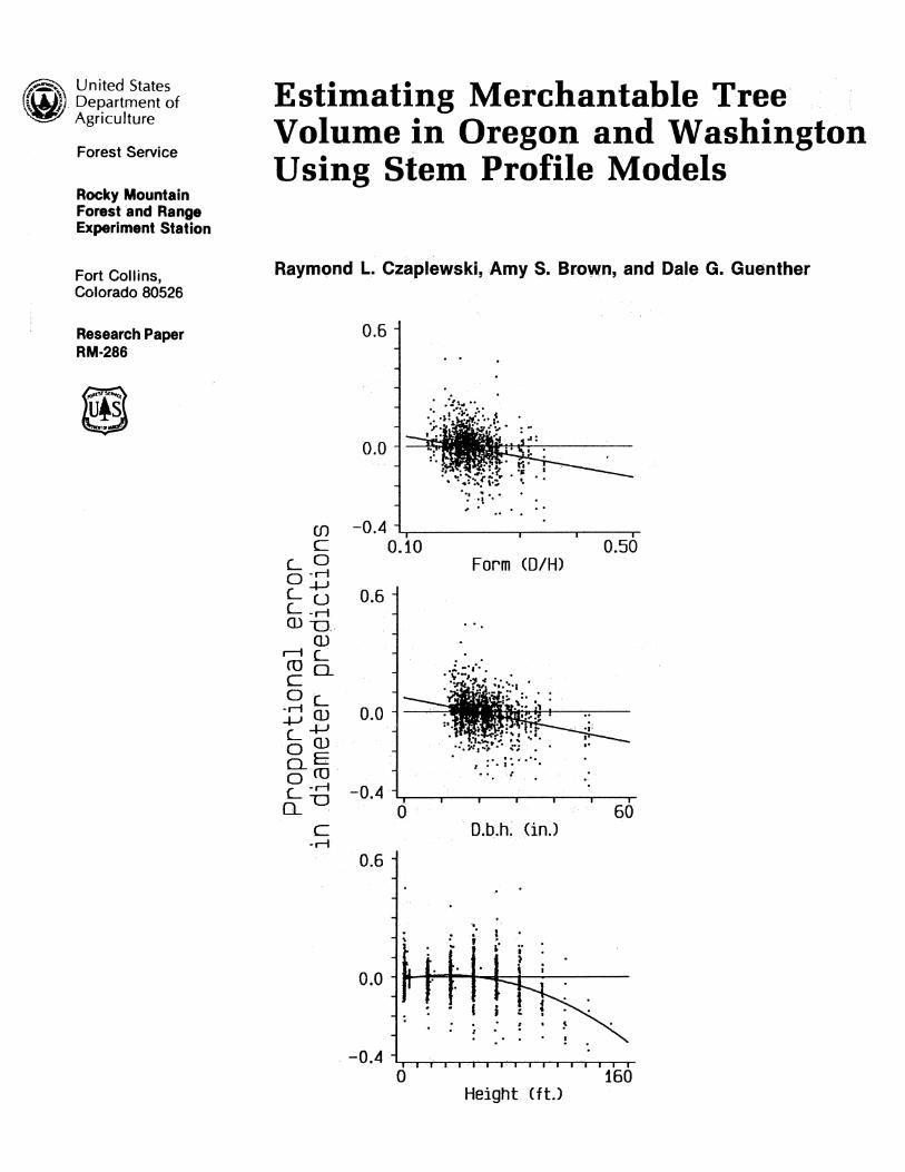
Residual errors from the Max and Burkhart model were weakly correlated with the following independent variables, as illustrated in figure 3: tree size (represented by D), an index of tree form (measured by DIH), and a curvilinear function of height (h) of the upper stem diameter prediction. The practical significance of these correlations with independent variables varied by tree species. The second-stage model reduces the bias in predicted diameter, but the standard deviations of the residuals for diameter predictions decreased only 3%.

The effect of the second-stage model on the represen- tation of tree form is not obvious. It is conceivable that the second-stage model produces illogical predictions of stem shape, especially for trees near extremes in the distribution of size and form. Therefore, the second-stage predictions of inside bark diameter (a,) were closely scrutinized for all trees in the data base. The multiplier that empirically corrects for bias, i.e., the bracketed por- tion in equation [3], does not greatly change the diameter estimate from the stem profile model. For all trees in this study, the extreme values were 0.71 and 1.10; 90°/o of the values were between 0.95 and 1.04, and half the values ranged between 0.98 and 1.01. The magnitude of these correction multipliers is similar to those found by Flewelling and Pienaar (1981) to correct for transforma-

tion bias in logarithmic volume equations. In addition, the second-stage diameter prediction (2,) is always positive and becomes smaller as height h increases for each tree. There were no unusual changes in the rate of stem taper for any tree, as evaluated using the second derivative of a, with respect to h (Czaplewski 1989); there were no stair-step patterns, i.e., sign reversals in the second derivative as h increased for any one tree. Therefore, the second-stage model produced logical diameter estimates for all trees. However, it is possible that the second-stage model could poorly represent the form of a tree if its d.b.h. and total height are not represented by the trees in the data base (see tables A1 through A7), and this potential, although unlikely prob- lem should be considered when the second-stage model is applied.

Predicting Diameter Outside Bark

The unbiased estimate of inside bark diameter a, at height h is used to predict diameter outside bark aOb at the same height:

where C, and c are regression parameters. Scatterplots of the ratio dpb/$, and the model for aobiaz (equation [5]), are shown in figure 4. Regression parameters were estimated using the following regression model:

Scatterplots of this transformation, and plots of the linear regression models (equation [6]), are given in figure 5. Estimated regression parameters and statistics are in table 3; the mean error for estimates of dob are within 0.63 inch of zero.

This model represents a function of bark thickness, and was chosen based on exploratory data analysis of the

Grand f i r 0.7

3' ' ' ' ' ' ' '1 . .

a,'" -0 I .d

F * -A g L a,= -P a,

5 % .d

a .d -a

a, L a

P a c i f i c s i l v e r f i r 0.6 0.6

. .. . . . I

, . ., . , .. -0.4 -0.4

0.10 0.50 D.b.h. (in.) Form (D/H)

0.0

. ' , -0.4

0 160 Height ( f t . )

Shasta fir

. 0.0 0.0

. .. ,

-0.4 -0.4 0 70 0.10 0.50

D.b.h. (in.) Form (D/H) 0.5

f . ' " ' : ' ' " ' " ' " ' ~

-0.4 0 170

Height ( f t .1

-0dgepole pine

0 70 l3.b.h. (in.)

. 0.0

-0.5 0 100

Height (ft.1

Douglas-f ir

0 230 Height t f t . )

0.10 0.70 Form (D/H)

0.10 0.70 Form (D/H)

0.0

-0.5 0 7 0

D.b.h. (in.) 0.7 f " " ~ " ' " ' ~ " " ' ~

Height (ft.,. -

Western l a r c h

0 60 D.b.h. (in.)

. 0.0

-0.5 0 150

Height ( f t . )

Ponderosa pine

0 7 0 D.b.h. ( in.)

. 0.0 . > ! # ! ; ;

-0.5 0 Height ( f t .1 150

Form (D/H)

i. ! 3' : .. . . . .. -0.5

0.10 0.50 Form (D/H)

Western hemlock 0.51' ' ' ' ,'. ' ' 1

. 0.0

-0.4 0 70

D.b.h. (in.) 0.5 ~ " " " " " ' " " " ' t . .

0.10 0.70 Form (D/H)

- 0.0

-0.4 0 180

Height ( f t . )

I n d e p e n d e n t p r e d i c t o r v a r i a b l e s

0.10 Form (D/H) 0.50

Figure 3.-Scatterplots of residual error in predicting diameter inside bark, using the Max and Burkhart model. The following independent variables are included: d.b.h. (D); an index of tree form, defined as d.b.h. divided by total tree height (DIH); and height of the diameter measure. ment (h). There are weak correlations of residuals with independent variables, which means that the stem profile model does not explain all patterns in the data. Regression models that predict residual error are given. These models use only one independent variable. Stepwise multiple regression models were fit to these residuals (table 2).

P a c l f l c s ~ l v e r f l r Grand f l r Shasta f l r

"M.,:, .* *w* r i .( ' . 1 0 1.0

.?" <,"-b

R Y 1 .o

L -0 (0 an 10 u 160 10 170 10 170 fi a,

Western l a r c h Lodgepole p ine 1.8

1 0 1.0 u E 4 m cn 4

150 10 180 10 150 m u

aJ Doug las - f l r Western hemlock

-CI .4 a,- 2 0

1.7

E a, ru L .,I a 0 .

1 0 1 .o

10 230 10 180

Helght from top of t r e e ( f t . ) Figure 4.-Scatterplot of ratio between diameter outside bark (do,,) and the unbiased predic-

tion of diameter inside bark (d ). Curves are fitted models, retransformed from the linear regression models that use log~(do,ld2) - I].

P a c l f l c s l l v e r f l r Grand f l r Shasta fir 0

7: ,.,r*>*- k., . 73 cn a 3

-2 f, Z E -7 -8 -6 u, 10 160 10 170 10 170

~2 L m Western l a r c h Lodgepole p lne Ponderosa p lne

0 , ' " '.rw,.<7*>dA% + ".

-CI rl 9 0 L

L $ -7 - 7 -7 m a ] 10 150 10 100 10 150

Western hemlock

10 230 10

Height from top of t r e e ( f t .1 Figure 5.-Scatterplots of transformed variable, i.e., log (do,,ld2 - I), used to fit model for

diameter outside bark, given an unbiased prediction of diameter inside bark. Fitted regression line is also portrayed.

Table 3.-Second-stage models for dob (equation 151) and a summary of errorsa in predicting upper stem outside bark diameters.

Mean Regression Regression residual statisticsb coefficientsC

Species n inches t- F Ft2 '6

stat. C7

Pacific silver fir 1,735 -0.01 0.40 41.77 0.03 -2.277948 -0.0049568 Grand fir 7,840 0.15 7.44 11.20 0.01 -2.119883 -0.0012616 Shasta fir 1,661 0.25 5.62 18.80 0.01 -1.856899 -0.0023925 Western larch 2,224 0.20 4.20 97.92 0.05 -2.609802 0.0074167 Lodgepole pine 5,877 -0.02 -1.16 385.15 0.08 -2.015476 -0.0091009 Ponderosa pine 10,194 0.06 5.03 180.30 0.02 -1.987724 -0.0043569 Douglas-fir 13,318 0.63 90.45 270.62 0.02 -1.740004 -0.0029642 Western hemlock 3,553 -0.01 -0.25 264.18 0.08 -1.931856 -0.0073768

aMean residual error is measured minus predicted dog (at stump, d.b.h., and end of merchantable 16-foot logs). t-statistic is the mean residual dinded by its standard error of the mean (dimensionless).

h he degrees of freedom for the F-statistic are (k-1, n-k-1) where k is the number of non-zero regression coefficients (including c,), and n is the number of observations.

'=Coefficient are dimensionless and were f i t using linear regression with a logarithmic transformation.

response variable (dobla2). This model form was selected A new model for predicting Girard form class was for four reasons. First, the variance of the response developed using the validation data. Therefore, compar- variable is homogeneous relative to h (fig. 5). Second, the isons between the Max and Burkhart and Behre models regression parameters C6 and c7 could be estimated us- are confounded by the lack of independence between the ing linear regression and a logarithmic transformation. validation data and predictions from the Behre models; Third, the model always predicts a diameter outside bark the accuracy of the Behre model is somewhat exag- that is larger than the estimated inside bark diameter gerated. However, this comparison is presented as the because exp[c6 + c,(H-h)]>O. Fourth, the estimated tip best possible. diameter is zero (aob = 0 for h = H) because a2 = o for h = H.

Validation Data

Independent Test

The preceding results describe fit of the Max and Burkhart and second-stage model diameters to the same data that were used to build the models. In the following test, these regional profile and second-stage models are applied to independent validation data from three national forests (i.e., a subregion of the entire study area). The validation data were not used to fit the Max and Burkhart and second-stage models. The accuracy of predicting merchantable volume, in addition to stem diameters, is evaluated.

Accuracy of the Max and Burkhart and second-stage models is also compared with the Behre profile model that is presently used in the Pacific Northwest, as given by Bruce (1972). The Behre profile model is

D(F/lOO)[I-(h-hf)l(h-h,)] a. = lb 1 + (c-l)(h-h,)/(H-h,)

where F is Girard form class, which is defined as the diameter inside bark at the top end of the first 16- or 32-foot log expressed as a percentage of d.b.h., hf is the height aboveground of the top of the first log, and c is a constant. Diameters below hf are not defined by the Behre model; however, a separate regression model has been fit by the Pacific Northwest Region to estimate stump diameter at 1 foot using d.b.h.

Data were gathered for the Deschutes National Forest lNFl in 1987. and the Mt. Hood and Siuslaw NF's in 1988. The' species sampled in the Deschutes NF were Shasta fir, grand fir, lodgepole pine, ponderosa pine, Douglas- fir, and western hemlock. On the Mt. Hood NF, Pacific silver fir, grand fir, western larch, lodgepole pine, ponderosa pine, Douglas-fir, and western hemlock were sampled. On the Siuslaw NF, two species were sampled: Douglas-fir and western hemlock. Additional species in each of the forests were sampled, but had small sample sizes, or were species that had no profile model; these were not used. The range, mean, and standard deviation for d.b.h. and total tree height are given for each species in the three forests in table 4.

A Tele-relaskop2 was used to make standing tree measurements of d.b.h. (D,), upper stem diameters (d,), and total tree height (H). Sightings were made at a variety of compass bearings. D.b.h. (D) was also measured with a diameter tape. Diameters were measured at heights that correspond to nominal 16- or 32-foot logs. Most Tele- relaskop diameter measurements at breast height were within 3% of the tape measurements. The tape and Tele- relaskop measurements of d.b.h. were compared (i.e., D and D,), and trees with a difference larger then 10% (i.e.,

*The use of trade and company names is for the benefit of the reader; such use does not constitute an official endorsement or approval of any service or product by the U.S. Department of Agriculture to the exclusion of others that may be suitable.

Table 4.-Means, standard deviations (SD), range, and number of trees measured (n) in the independent test data, grouped by d.b.h. and total tree height by species and forest.

National forest species

Deschutes Grand fir Shasta fir Lodgepole pine Ponderosa pine Douglas-fir Western hemlock

Mt. Hood Pacific silver fir Grand fir Western larch Lodgepole pine Ponderosa pine Douglas-fir Western hemlock

Siuslaw Douglas-fir Western hemlock

No. trees

No. sections

D.b.h. (feet) Mean SD Min. Max.

Total tree height (inches) Mean SD Min. Max.

(D,-D)ID>O.10) were omitted. The remaining data were calibrated for measurement differences between tape and sighted data. The calibrated diameter outside bark (doh) was computed as follows:

Log length and end diameters outside bark (doh) that cor- responded to the Tele-relaskop measurements were entered into standard scaling algorithms used by the USDA Forest Service in the Pacific Northwest Region to compute measured cubic volume inside bark using Smalian's formula.

Standing Tree Estimate of Form Class

Girard form class is needed to apply the Behre profile model as implemented in the Pacific Northwest Region. Traditionally, form class for standing trees had been ocularly estimated on the three NF's from which validation data were collected. However, it was suspected that a prediction model, using d.b.h. and total height, might be a more accurate estimator of Girard form class. A prediction model for form class was fit using the independent validation data.

Two predictor variables were available to estimate Girard form class; diameter at breast height (D) and total tree height (H). The regression model used Girard form class (F) as the dependent variable, which has units of percentage of d.b.h. Several transformations of the predictor variables were explored: D, H, lID, lIH, log(D), and log(H). 1ID and IIH accounted for the most varia- tion. The selected prediction equation was:

where c8, c?, and clo are regression coefficients. This model was fit using step-wise regression, and estimated model parameters are given in table 5.

Comparison of Profile Models

The Behre model predicted diameter inside bark with mean errors ranging from -0.61 to 0.72 inch (table 6) depending upon species and national forest. The mean error for the Max and Burkhart model ranged between -1.43 and 0.33 inches. However, this difference in bias could be caused by applying a regional model (i.e., the Max and Burkhart model with parameter estimates in tables 1 and 2) to a subregional data set. When the Max and Burkhart model was fit with the same data used for the form class model for the Behre profile model, the Max and Burkhart model was less biased (table 6) than the Behre model.

Table 7 compares the Max and Burkhart and second- stage models with the Behre model. However, predictions of cubic volume, rather than log end diameters, are used as the evaluation criterion. The predicted diameters at log ends are used to compute cubic volume using algorithms implemented by the Forest Service. The Max and Burkhart model had mean errors between -18.7% to 4.2%, with one-third of the mean errors within 2% of zero. The Behre model had less mean error in volume prediction; mean error ranged from -14.1°/o to 5.2% but more than half the mean errors were within 2.0% of zero. The Behre profile model uses a prediction of Girard form class, which was fit with the same data that is used to evaluate differences in volume estimates. Therefore, the Behre model is more accurate in this evaluation than can be normally expected, which confounds the assessment of this model.

For Douglas-fir on the Siuslaw NF, both profile models had relatively large mean errors in volume predictions, with the Max and Burkhart model overestimating volume by 10.9%, and the Behre model overestimating volume by 14.1% (table 7). However, both models had mean errors for Douglas-fir from the Mt. Hood and Deschutes NF's that were much closer to zero. For

Table 5.-Residual error summary, regression statistics, and regression coefficients for the Girard form class model (equation [a]). Validation data were used to estimate parameters.

Residual Regression Regression erroP statistics coefficientsb

National forest t - species stat. RMSE R~ C8 Cg C1o

Deschutes Grand fir Shasta fir Lodgepole pine Ponderosa pine Douglas-fir Western hemlock

Mt. Hood Grand fir Pacific silver fir Western larch Lodgepole pine Ponderosa pine Douglas-fir Western hemlock

Siuslaw Douglas-fir Western hemlock

aThe range of the mean residual errors was 0.000727 to -0.0007 77 except for Douglas-fir in the Siuslaw with a residual error of 0.83235%.

b ~ h e dimensions of regression coefficients are: cB, dimensionless constant; cg, (ft-'), and clo (in-').

Table 6.-Comparison of Max and Burkhart and Behre di, estimates with validation data.

Max and Burkhart and Behre model Max and Burkhart and second-stage models fit to second-stage models

fit to regional data validation model fit to validation data National No. of No. of Mean t- Mean t- Mean t- forest trees sections error stat. error stat. error stat.

(inches) (inches) (inches)

Deschutes Grand fir Shasta fir Lodgepole pine Ponderosa pine Douglas-fir Western larch

Mt. Hood Shasta fir Pacific silver fir Western larch Lodgepole pine Ponderosa pine Douglas-fir Western hemlock

Siussaw Douglas-fir Western hemlock

aNo second-stage model found.

9

Table 7.-Comparison of average percentage differences in merchantable board foot volume estimates for the Max and Burkhart and second-stage models, and the Behre model, using independent validation data. Negative values indicate overestimates of volume.

Max and Burkhart model Behre model Max and Burkhart model vs. true cubic volume vs. true cubic volume vs. Behre model

Cubic foot volume Cublc foot volume Cubic foot volume

No. of Mean cubic Percent Mean Residual t. Percent Mean Residual t. Percent Mean Residual t- trees vol. per tree error error SD stat. error error SD stat. error error SD Stat.

Deschutes N F Grand fir California red fir Lodgepole pine Ponderosa pine Douglas-fir Western larch

Mt. Hood N F Shasta fir Pacific silver fir Western larch Lodgepole pine Ponderosa pine Douglas-fir Western hemlock

Siuslaw N F Douglas-fir Western hemlock

western larch from the Deschutes NF, both models overestimated volume by an average of over 13% (table 7). However, both models had mean errors within 2% for western larch from the Mt. Hood NF. Max and Burkhart model overestimated volume of western hemlock from the Siuslaw NF by an average of 13.8%, whereas the Behre model was much less biased. However, bias of the Max and Burkhart model was much less for western hemlock on the Mt. Hood NF, with a mean error of -1.3%. The Max and Burkhart model tended to overestimate volume of ponderosa pine by an average of 12.6% on the Deschutes NF, and 9.7% on the Mt. Hood NF. The Behre model had less bias for ponderosa pine volume (table 7). All other differences in mean error of volume estimates (table 7) were smaller for both models.

The Max and Burkhart model is not expected to produce merchantable volume estimates that are radically different from the Behre model, which is currently used in practice. The differences in volume predictions between models are compared in table 7. On the average, differences between models were less than 10% for all but four cases. The greatest differences between models were in predictions of merchantable volume for western larch (16.4%) on the Deschutes NF, although differences were much less on the Mt. Hood NF (1.8%). There were also differences for ponderosa pine; volume predictions from the Max and Burkhart model were larger than those from the Behre model by an average of 10.2% for the Mt. Hood NF, and 12.6% for the Deschutes NF. The Max and Burkhart model also produced larger volume estimates (13.5%) for western hemlock on the Siuslaw NF, although the two models were in much closer agreement for western hemlock on the Mt. Hood NF (1.3%). Therefore, in most cases, the Max and Burkhart model can be expected to produce volume estimates similar to those from

the currently used Behre model, without the accurate standing tree estimates or predictions of Girard form class that are needed by the Behre model.

Discussion

One of the purposes of the second-stage model is to adjust for bias in predicted diameter from the Max and Burkhart model that is manifested during the retransformation of estimated (d+lD)' to estimates of dib: The transformation (dib/D) 1s used to stabilize variance,

which is required when using traditional (i.e., unweighted) regression techniques. The squaring of this transformation [i.e., (dib/D)'] increases precision of the volume estimates and reduces the nonlinearity of the profile model while continuing to stabilize variance. Diameter (dib) could be used directly as the response variable in the regression model, and this would avoid overall retransformation bias. However, the variance of the residuals would be dependent on diameter, d.b.h., and measurement height, which violates the assumptions in the usual ordinary least squares linear regression model. Also, more weight would be placed on minimizing prediction errors for large trees, and diameters near the base of the tree, because the magnitude of the errors would be larger. Conceivably, this could produce models that predict negative upper stem diameters, or poorly represent smaller trees. The (dib/D) or (dib/D)' transformations put smaller on a more equal metric with the larger trees and lower stem measurements. The (dib/D) transformation could have been used in place of the (diblD)' transformation, but this would have introduced additional nonlinearities into the regression model, and would have imposed additional costs. Weighted regression could also be used to more directly treat the

heteroscedasticity of dib. Carrol and Ruppert (1988) provide a recent summary of the relevent literature. However, elimination of the correlations of residuals with D and DIH (figs. 3 and 4) likely requires more than weighted regression.

The second-stage models correct for mean errors of 0.06 to 0.24 inch in diameter predictions; these systematic biases, although relatively small, can translate into substantial volume estimation errors when applied to a large geographic region. It is difficult to defend overestimation of merchantable volume, especially when the bias is easy to correct empirically on the average. However, the bias for any one timber sale can be high, even when using a model that is unbiased for a large region. There is naturally high variability in stem form at the local level, and there is no inexpensive way to measure this variablity so that every local estimate is unbiased. Even so, the second-stage model, which contains a covariate of tree form (i.e., DIH), can improve local estimates (Czaplewski et al. 1989).

As precision of the diameter predictions improves, in- dividual diameter estimates from an unbiased model will be closer to their true values. The predictor variables in the second-stage model (i.e., D, DIH, h, h2) improve precision; the standard deviation of residuals from the second-stage model for all trees in the appendix is 3% less than that from the stem profile models alone.

The risk of using the second-stage model is small. Residuals from the second-stage models have been closely scrutinized, and no problems have been detected. Cer- tain problems, which are possible, although unlikely, can be readily checked when the second-stage models are applied in practice. These checks are simple to implement; e.g., verify that diameter estimates are positive and decrease going up the main stem. Also, both the old volume estimators and new ~rof i le models can be used during a trial period; if thereare unidentified risks, then they will probably surface during a trial period. Risks of not using the second-stage models are larger. For ex- ample, overestimates of merchantable volume for large geographic areas from the unadjusted Max and Burkhart model could distort analyses in forest management plans.

Emphasis has been placed on minimizing bias in predictions of upper stem diameters, even though volume estimation is the final goal. It is common practice in research studies to integrate stem profile models to estimate cubic volume (Martin 1981). However, the Forest Service and many other forest management organizations use log length and log end diameters to scale (i.e., estimate) merchantable log volume. Also, merchantable board foot volume is defined primarily by the upper end diameter estimate, rather than the integrated cubic volume estimate. Even in detailed stem analysis studies, section lengths and end diameters are usually measured to indirectly estimate cubic volume (e.g., Smalian's formula); water displacement methods are seldom used to measure volume directly (Martin 1984). Therefore, integrated cubic volume estimates might not represent the same definition of volume that is used in the field.

Cubic volume estimates from section length and predicted end diameters will differ slightly from cubic volume estimates obtained from integrating the stem profile model. However, it is prudent to maintain consistency in volume estimation for timber sale preparation, log scaling, inventory, and planning. Therefore, the stem profile and second-stage models are used to predict the number of merchantable logs in a tree, and diameters at heights that correspond to log ends. These predictions are entered into existing algorithms to scale merchantable log volume. This increases the data processing load, but internal flexibility and consistency are maintained. Similar procedures have been used for decades in the Pacific Northwest by both forest industry and govern- ment land management agencies. Scaled cubic volume from a profile model will be highly correlated with integrated cubic volume from the same model.

Without the second-stage model, the Max and Burkhart stem profile model can readily estimate diameters at given heights, heights to given top diameters, and cubic volume of stem sections. Although this provides con- siderable convenience, many of these predictions con- tain bias. However, the second-stage model can produce approximately unbiased estimates of stem diameter. Presumably, this will reduce bias in predictions of merchantable height (at the cost of increased computations), and volume predictions that use diameter predictions from the second-stage model as input variables to scaling algorithms. Therefore, the second-stage model can provide both mensurational and institutional benefits.

The stem profile models in this paper are expected to provide useful predictions of merchantable volume given a variety of merchantability standards and scaling rules. These predictions are expected to be unbiased, when many local sites are averaged together, and when applied to the same population of trees (see appendix) that were used to estimate regression parameters. It is not known how well these models will predict diameters for trees from other populations. The distribution of tree form and size can change over time, especially for second-growth stands, and new stem profile models will be required at some time in the future.

Acknowledgments

John Teply originally proposed that emphasis be placed on unbiased predictions of diameter, rather than other estimates that can be produced from a stem profile model. Tim Max suggested substantial improvements in the development and verification of the second-stage model. David Bruce enriched our critical examination of the methods and interpretations.

Literature Cited

Alberta Forest Service. 1987. Evaluation and fitting of tree taper functions for Alberta. Pub. No. Dept. 106. Edmonton, AB: Silva Com. Ltd. 148 p.

Amidon, E. L. 1984. A general taper functional form to predict bole volume for five mixed-conifer species in California. Forest Science. 30: 166-171.

Behre, C. E. 1923. Preliminary notes on studies of tree form. Journal of Forestry. 21: 507-511.

Bruce, D. 1972. Some transformations of the Behre equation of tree form. Forest Science. 18: 164-166.

Cao, V. Q.; Burkhart, H. E.; Max, T. A. 1980. Evaluation of two methods for cubic volume prediction of loblolly pine to any merchantable limit. Forest Science. 26: 71-80.

Carroll, Raymond J.; Ruppert, David. 1988. Transforma- tion and weighting in regression. New York, NY: Chap- man and Hall.

Czaplewski, R. L. 1989. Graphical analysis of stem taper in model building. Canadian Journal of Forest Research. 19: 522-524.

Czaplewski, R. L.; Brown, A. S.; Walker, R. C. 1989. Stem profile models in Wyoming, Colorado, and South Dakota. Res. Pap. RM-284. Fort Collins, CO: U.S. Department of Agriculture, Forest Service, Rocky Mountain Forest and Range Experiment Station. 7 p.

Draper, N. R.; Smith, H. 1981. Applied regression analysis. New York, NY: John Wiley and Sons. 709 p.

Flewelling, J. W.; Pienaar, L. V. 1981. Multiplicative regression with lognormal errors. Forest Science. 27: 281-289.

Gordon, A. 1983. Comparison of compatible polynomial taper equations. New Zealand Journal of Forestry Science. 13: 146-153.

Maguire, D. A.; Hann, D. W. 1987. Equations for predicting sapwood area at crown base in southwestern Oregon Douglas-fir. Canadian Journal of Forest Research. 17: 236-241.

Martin, A. J. 1981. Taper and volume equations for selected Appalachian hardwood species. Res. Pap. NE-490. Broomall, PA: U.S. Department of Agricul- ture, Forest Service, Northeastern Forest Experiment Station. 22 p.

Martin, A. J. 1984. Testing volume equation accuracy with water displacement techniques. Forest Science. 30: 41-50.

Max, T. A.; Burkhart, H. E. 1976. Segmented polynomial regression applied to taper equations. Forest Science. 22: 283-289.

Sterba, H. 1980. Stem curves--a review of the literature. Forestry Abstracts. 41: 141-145.

Taylor, J. M. G. 1986. The retransformed mean after a fitted power transformation. Journal of American Sta- tistical Association. 81: 114-118.

Appendix

Table A1.-Number of trees for Pacific silver fir.

Region D.b.h. class (inches) Total height class (feet) Total National Forest 7-11.9 12-13.9 14-14.9 15-16.9 17-19.9 20-22.9 23-48.9 35-59.9 60-69.9 70-79.9 80-84.9 85-99.9 100-114.9 115-170 trees

Northwestern Oregon & Southern Washington GiffordPinchot 2 12 12 35 38 32 20 2 9 47 14 29 36 14 151 Mt. Hood 0 8 3 16 13 10 24 0 1 17 8 19 8 21 74 Willamette 1 4 3 9 18 9 15 0 2 10 8 17 13 9 59

Total 3 24 18 60 69 51 59 2 12 74 30 65 57 44 284

Table A2.-Number of trees for grand fir.

Region D.b.h. class (inches) Total height class (feet) Total National Forest 7-13.9 14-16.9 17-18.9 19-21.9 22-24.9 25-28.9 29-56 35-59.9 60-69.9 70-79.9 80-84.9 85-94.9 95-109.9 110-205 trees

Central Oregon Deschutes 19 25 18 28 29 25 16 22 24 38 11 32 23 10 160 Fremont 3 19 13 24 27 48 35 43 28 37 10 34 15 2 169 Winema 43 35 14 16 24 19 32 48 21 29 9 21 22 33 183

Total 65 79 45 68 80 92 83 113 73 104 30 87 60 45 512 Eastern Oregon

Malheur 10 32 34 40 26 20 14 45 34 34 18 22 14 9 176 Ochoco 18 23 20 24 20 23 10 29 26 21 11 27 17 7 138 Umatilla 48 33 29 33 21 23 22 29 30 30 21 40 31 28 209 Wallowa-Whitman 20 15 17 22 22 29 42 28 20 20 12 19 40 28 167

Total 96 103 100 119 89 95 88 131 110 105 62 108 102 72 690 Northwestern Oregon & Southern Washington

Mt. Hood 24 1 0 0 0 0 0 7 7 4 5 2 0 0 25 Southwestern Oregon

Rogue River 30 32 12 29 29 38 50 36 29 17 15 30 30 63 220 Grand Total 215 215 157 216 198 225 221 287 219 230 112 227 192 180 1,447

Table A3.-Number of trees for Shasta fir.


Central Oregon Winerna 25 31 15 15 8 0 0 39 21 25 6 3 0 0 94

Southwestern Oregon Rogue River 7 16 20 22 36 34 44 11 9 23 32 34 39 31 179

Grand Total 32 47 35 37 44 34 44 50 30 48 38 37 39 31 273

Table A4.-Number of trees for western larch.


Eastern Oregon Umatilla 29 33 34 47 19 14 9 53 36 25 21 27 8 15 185 Wallowa-Whitman 14 11 22 25 32 31 51 19 21 22 26 30 39 29 186

Total 43 44 56 72 51 45 60 72 57 47 47 57 47 44 371

Table A5.-Number of trees for lodgepole pine.

Region D.b.h. class (inches) Total height class (feet) Total National Forest 6-8.9 9-9.9 10-10.9 11-11.9 12-13.9 14-15.9 16-27 40-49.9 50-54.9 55-59.9 60-64.9 65-74.9 75-105 trees

Central Oregon Deschutes Frernont Winerna

Total Eastern Oregon

Urnatilla Northwestern Oregon

Gifford Pinchot Mt. Hood Siuslaw Willarnette

Total Grand Total

43 26 30 & Southern Washington

0 2 4 0 0 0 0 0 0 0 1 4 0 3 8

51 76 110

Table A6.-Number of trees for ponderosa pine.


Central Oregon Deschutes Frernont Winerna

Total Eastern Oregon

Malheur Ochoco Urnatilla Wallowa-Whitrnan

Total Northwestern Oregon

Mt. Hood Grand Total

34 29 18 35 27 26 33 17 36 19 38 20 33 22 26 34 29 49 66 52 31 36 45 23 37 41 36 36

113 144 89 159 154 147 122 & Southern Washington

10 16 22 21 31 41 44 210 280 184 263 302 250 246

Table A7.-Number of trees for Douglas-fir.


Central Oregon Deschutes 12 19 30 35 30 24 10 20 29 48 38 13 12 0 160

Eastern Oregon Ochoco 21 40 36 24 29 23 6 51 44 41 36 6 1 0 179 Urnatilia 45 51 55 28 26 6 2 101 49 31 18 8 5 1 213

Total 66 91 91 52 55 29 8 152 93 72 54 14 6 1 392 Northwestern Oregon & Southern Washington

Gifford Pinchot 27 29 25 19 23 28 31 15 37 28 28 30 30 14 182 Mt. Hood 80 63 48 55 59 54 56 71 81 79 70 38 43 33 415 Siuslaw 28 49 37 48 58 61 43 7 7 16 42 54 92 106 324 Willarnette 12 13 31 26 28 29 31 9 15 17 24 27 32 46 170

Total 147 154 141 148 168 172 161 102 140 140 164 149 197 199 1,091 Southwestern Oregon

Siskiyou 10 14 20 20 23 40 53 6 13 19 22 29 47 44 180 Grand Total 235 278 282 255 276 265 232 280 275 279 278 205 262 244 1,823

Table A8.-Number of trees for western hemlock.

Region D.b.h. class (inches) Total height class (feet) Total

National Forest 9-13.9 14-16.9 17-18.9 19-22.9 23-26.9 27-33.9 34-57 40-74.9 75-89.9 90-99.9 100-109.9 110-124.9 125-139.9 140-195 trees

Northwestern Oregon & Southern Washington GiffordPinchot 21 23 22 31 31 19 30 37 29 22 29 26 16 18 177 Mt. Hood 21 34 23 22 16 32 31 28 35 25 20 19 21 31 179 Siuslaw 0 0 0 0 0 3 0 0 0 0 0 0 1 2 3 Willamette 22 19 16 43 30 25 17 21 30 20 22 30 26 23 172

Grand Total 64 76 61 . 9 6 77 79 78 86 94 67 71 75 64 74 531

I

Czaplewski, Raymond L.; Brown, Amy S.; Guenther, Dale G. 1989. I Estimating merchantable tree volume in Oregon and Washington I using stem profile models. Res. Pap. RM-286. Fort Collins, CO: U.S. I Department of Agriculture, Forest Service, Rocky Mountain Forest I and Range Experiment Station. 15 p. I

I The profile model of Max and Burkhart was fit to eight tree species I

in the Pacific Northwest Region (Oregon and Washington) of the I Forest Service. Most estimates of merchantable volume had an average I error less than 10°/o when applied to independent test data for three I national forests. I

I Keywords: Taper equations, merchantable volume estimates, bias cor- I rection, Abies amabilis, Abies grandis, Abies magnifica, Larix occiden- I talis, Pinus contorta, Pinus ponderosa, Pseudotsuga menziesii, Tsuga I heterophylla I

U.S. Department of Agriculture Forest Service

Rocky Mountain Forest and Range Experiment Station

The Rocky Mountain Station is one of eight

Rocky regional experiment stations, plus the Forest Products Laboratory and the Washington Office

Mountains Staff, that make up the Forest Service research organization.

RESEARCH FOCUS

Research programs at the Rocky Mountain Station are coordinated with area universities and with other institutions. Many studies are conducted on a cooperative basis to accelerate solutions to problems involving range, water, wildlife and fish habitat, human and community development, timber, recreation, protection, and multiresource evaluation.

Southwest RESEARCH LOCATIONS

Research Work Units of the Rocky Mountain Station are operated in cooperation with universities in the following cities:

Albuquerque, New Mexico Flagstaff, Arizona Fort Collins, Colorado * Laramie, Wyoming Lincoln, Nebraska

Great Rapid City, South Dakota Tempe, Arizona

Plains

'Station Headquarters: 240 W. Prospect Rd., Fort Collins, CO 80526

estimating merchantable tree volume in oregon and ... · burkhart model was more precise and...

Documents