estimating beta - bgushalit/publications/beta_rqfa.pdf · review of quantitative finance and...

Review of Quantitative Finance and Accounting, 18: 95–118, 2002©C 2002 Kluwer Academic Publishers. Manufactured in The Netherlands.

Estimating Beta

HAIM SHALIT∗Department of Economics, Ben-Gurion University of the Negev, Beer Sheva, 84105 IsraelE-mail: [email protected]

SHLOMO YITZHAKIDepartment of Economics, Hebrew University of Jerusalem, Jerusalem, 91000 Israel and Director,Central Bureau of Statistics, Jerusalem, 91342 IsraelE-mail: [email protected]

Abstract. This paper presents evidence that Ordinary Least Squares estimators of beta coefficients of majorfirms and portfolios are highly sensitive to observations of extremes in market index returns. This sensitivity isrooted in the inconsistency of the quadratic loss function in financial theory. By introducing considerations of riskaversion into the estimation procedure using alternative estimators derived from Gini measures of variability onecan overcome this lack of robustness and improve the reliability of the results.

Key words: OLS estimators, systematic risk, mean-Gini

JEL Classification: G12

1. Introduction

The valuation of risky assets is one of the major research tasks in financial economics thathas led to the development of several Capital Asset Pricing Models, the most popular ofwhich is the Sharpe-Lintner-Black mean-variance CAPM. In this model, the typical measureof asset riskiness is the beta, i.e., the covariance between the asset return and the marketportfolio return. The basic tenet of CAPM lies in the separation of estimating beta riskfrom its pricing. Indeed CAPM assumes that one can define and measure systematic riskirrespective of risk aversion, which affects only the equilibrium pricing of individual assets.As is well known, this separation is valid only under the restrictive assumption of two-factorseparating distributions or alternatively, if the utility function is quadratic.

Empirical asset-pricing models attract massive attention in finance, their goal being toassert or refute whether CAPM holds true. The traditional technique used to estimate therisk-expected return relation consists of two stages. In the first pass, betas are estimated froma time-series. In the second pass, the relationship between mean returns and betas is testedacross firms or portfolios. This methodology has been the subject of much criticism that has

∗Address correspondence to: Haim Shalit, Department of Economics, Monaster Center for Economic Re-search, Ben-Gurion University of the Negev, Beer Sheva, 84105 Israel. Tel.: +972-8-6472299; Fax +972-8-6472941. E-mail: [email protected]

96 SHALIT AND YITZHAKI

led to many attempts at improvement. Such studies were initiated by Fama and MacBeth(1973) who introduced a rolling technique, and were followed by proponents of maximumlikelihood estimation, for example Gibbons (1982), Stambaugh (1982), and Shanken (1992)to name a few. MacKinlay and Richardson (1991) developed a test for mean-varianceefficiency without assuming normally distributed asset returns. However, CAPM suffered amajor setback due to a series of papers published by Fama and French (1992, 1993, 1995,1996, and 1997) who claimed that beta itself is not sufficient for explaining expected return.On the other hand, using alternative econometric and experimental techniques, Amihud,Christensen and Mendelson (1992), Jagannathan and Wang (1996), and Levy (1997) rejectedFama and French results and reclaimed beta as the valid measure of risk in asset pricing.All these findings point to a major question: Is beta relevant in finance or is it merelymis-estimated?

Since its inception in finance, beta has been used mainly for two purposes. The firstinvolves the ranking of assets and portfolios with respect to systematic risk by practition-ers. The second deals with testing CAPM and mean-variance efficiency. The latter processinvolves a second stage regression (cross-section regression) intended for testing the ef-ficiency of the market portfolio and the linear relationship between expected returns andbetas, as discussed for example by Kandel and Stambaugh (1995).

An additional issue that complicates the problem of estimating beta is that one cannotseparate the issue of risk aversion from the statistical loss function used in the estimation. Aswill be argued later, risk aversion signifies the asymmetric treatment of deviations from theregression of stock returns on market returns. On the other hand, statistical theory impliesthe equal treatment of observations. The clash between financial and statistical theoriescomplicates the estimation procedure, and therefore, we restrict our study to estimatingassets’ riskiness and delay the pricing of risk to further research.

In this paper we question whether the standard procedure for estimating systematic riskis compatible with financial theory and show how the regression technique used to estimatesystematic risk is not robust with respect to wide market fluctuations. The sensitivity ofbeta to the presence of extreme observations can give rise to data mining and lead the wayto peculiar relationships.

We argue that beta sensitivity can be traced to a combination of two factors:

(i) Incompatibility between standard statistical methods and financial theory. In parti-cular, the Ordinary Least-Squares (OLS) regression estimator is based on a quadraticweighting scheme that tends to contravene the assumptions of risk aversion;

(ii) Probability distribution of market returns with “fat” tails; that is the data do not followa normal distribution.1

Accordingly, these factors make beta sensitive to market fluctuations and therefore OLS isinappropriate for estimating betas.

We suggest alternative estimators for beta that are robust with respect to extreme fluctua-tions in the market return. In this sense, we follow Chan and Lakonishok (1992) and Knez andReady (1997) for the use of robust estimation procedures, but with a different rationale. Inusing trimmed regressions to seek robustness, crucial information regarding the behavior of

ESTIMATING BETA 97

securities returns with respect to market portfolio is removed for the sake of robustness. Thedata that becomes deleted may be considered by some investors as the most valuable becauseit represents information about the state of nature that concerns them the most. Therefore, wedo not seek robustness by using statistical methods that are less sensitive to generallywide fluctuations. Rather, we seek to identify, according to economic theory, the relativeweights that should be attached to different fluctuations. Adjusting the weighting schemefollowing economic theory allows for improving the systematic risk estimator at low cost.

To document the magnitude of the sensitivity of beta to market fluctuations and to avoidany influence of small or unusual companies, we first consider the 30 firms in the DowJones Industrial Average (DJIA) and then, 20 portfolios that have been built with the 100largest traded firms. We use CRSP daily returns for a period of ten years (January 1984through December 1993) making a total of 2528 observations. The use of the daily returnswas guided by two motivations:

(i) Daily returns provide a relatively large amount of data. Since we are interested in theeffect of extreme observations on the estimates, such as those that appeared duringthe 1987 Crash, a large amount of data will reduce the effect of any one observation.Ignoring the 1987 Crash altogether would imply that periods of high volatility do notplay an important role in any estimate;

(ii) Monthly returns are obtained by averaging daily returns. Thus they are expected todeviate from normality less than daily returns do.2 But as pointed out by Levy andSchwartz (1997), the longer the measurement period the lower will be the observedcorrelations among asset returns. Also, Levhari and Levy (1977) discuss the effect of theinvestment horizon on the empirical testing of beta. Hence, increasing the measurementperiod may “normalize” the distributions but at the same time will reduce the correlationamong the returns which defeats the main goal in estimating beta.

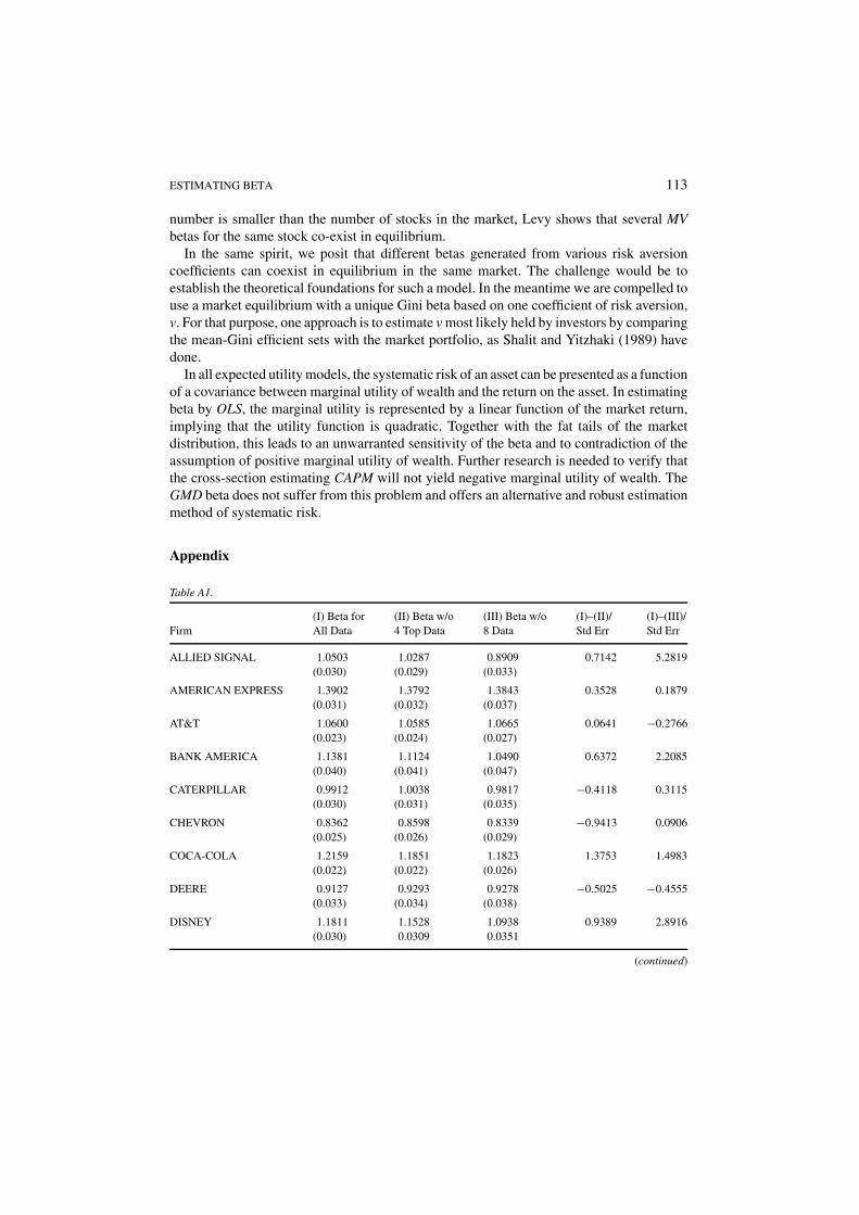
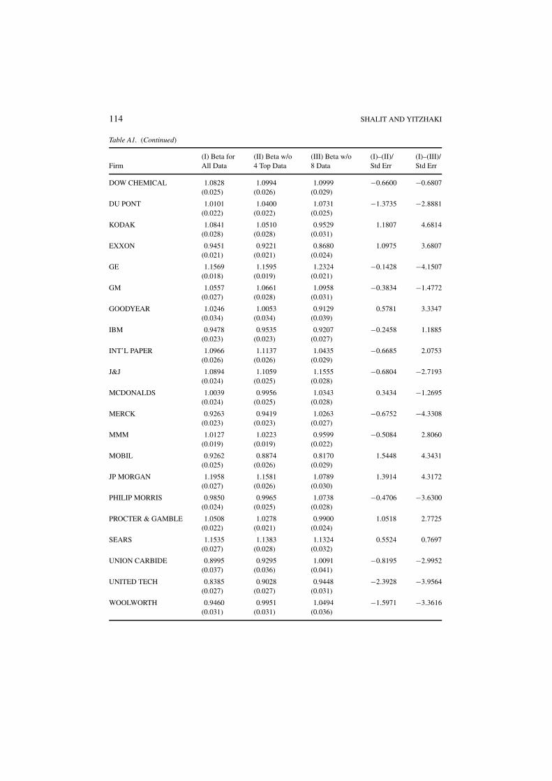
Using these data, we conduct two experiments. In the first, the highest four marketperformance observations based on the S&P 500 Index are removed from the sample andthe betas are re-estimated. In the second, the highest four and the lowest four observations ofthe market are deleted (a total of less than 0.3 percent of the entire number of observations).Table 1(a) reports the deviations of the new estimates of betas in terms of their standarderrors.3

When the highest four and the lowest four market returns are removed, the betas of 7 firms(out of 30) change by more than 4 standard errors. Moreover, the betas of more than 75% ofthe firms change by more than one standard error. When only the highest four observationsare omitted, then the betas of 9 firms (30 percent of the firms) change by more than onestandard error. However, the impression one gets from the standard errors using the entiresample, as reported in the Appendix, is that the probability of such occurrences is zero.

In Table 1(b), these same conclusions are also obtained with beta ranked portfolios that re-duce the problem of sharp return fluctuations for individual firms. When the highest four andlowest four market returns are omitted, the betas of 7 portfolios (out of 20) change by morethan 3 standard errors. When the highest four observations are deleted, the betas of 9 port-folios change by more than one standard error, confirming the results for individual stocks.


Table 1a. Number of DJIA 30 firms whose betas change according to magnitude of change

Magnitude of Change in β in Terms of Omitting 4 Highest Omitting 4 HighestStandard Error of the Estimate Returns & 4 Lowest Returns

Total number of firms 30 30Less than 1 standard error 21 7More than 1 and less than 2 standard errors 8 4More than 2 and less than 3 standard errors 1 8More than 3 and less than 4 standard errors 0 5More than 4 standard errors 0 7

Table 1b. Number of portfolios whose betas change according to magnitude of change∗

Magnitude of Change in β in Terms of Omitting 4 Highest Omitting 4 HighestStandard Error of the Estimate Returns & 4 Lowest Returns

Total number of portfolios 20 20Less than 1 standard error 11 6More than 1 and less than 2 standard errors 9 6More than 2 and less than 4 standard errors 0 7More than 4 standard errors 0 1

∗Twenty portfolios, each composed of 5 firms are built by ranking the largest 100 traded firms according to theirbetas. Detailed results are given in Table A2.

These results indicate beta’s great sensitivity to extreme market fluctuations, which castsdoubts on the robustness of the CAPM as it varies with respect to the choice of the sampleperiod and the specification of the model. This sensitivity exists for both upward anddownward movements of the market. Sensitivity to extreme downturn market fluctuationscan be justified by arguing extreme cases of risk aversion, but it is not easy to explainsensitivity to extreme upward market movement.

The aim of this paper is to explore those factors that contribute to the sensitivity of betaestimates to extreme observations of market returns and to suggest alternative estimators thatare both robust and better represent investors’ risk aversion. In particular, the analysis showsthat all models that represent the investor as an expected utility maximizer characterizesystematic risk by a covariance formula between the marginal utility of wealth and the asset’sreturn. The differences among the various models have to do with the exact specification ofthe marginal utility of wealth. Since this covariance cannot be observed, valuation modelsidentify risk by a specific measure of variability, like the variance or the semivariance,and for the latent covariance substitute a covariance between the market portfolio and anasset’s return. On the other hand, it is shown that the regression technique used to estimatesystematic risk implicitly specifies the functional form of the marginal utility of income,and thus determines the implied risk aversion.

The paper is organized as follows. Section 2 presents the OLS estimator for beta as aweighted average of the change in asset return conditional on the change in market returns.

ESTIMATING BETA 99

The weights used in averaging depend solely on the distribution of market returns. As theweights are sensitive to extreme market fluctuations, the OLS estimation procedure attachesgreater weights to extreme market changes, a characteristic that may contradict financialtheory.

In Section 3, we show how financial theory implies that systematic risk is expressed by acovariance formula between the marginal utility of wealth and asset return. Provided that theutility function is known, this covariance defines the ideal beta, that is the beta that would bemost suitable for reflecting the riskiness of the asset. Having defined the ideal beta enablesus to compare alternative estimators of beta with the ideal beta. This comparison reveals thatwhile it may be justified to attach greater weights to extreme downturn realizations of themarket, it contradicts financial theory to attach greater weights to upward movements ofthe market. The property of attaching heavy weights to extreme positive high returns on themarket portfolio challenges financial theory and simultaneously decreases the robustnessof the estimator of beta.

In Section 4, we offer alternative estimators for describing the riskiness of an asset such asthe extended Gini estimators, and investigate their properties. These estimators attach lowerweights than the OLS estimators to upward market movements, thus making the estimatorboth more appropriate from the theoretical point of view, and at the same time more robustthan the OLS estimator. Section 5 concludes the paper.

2. The OLS estimator for beta

We introduce the OLS estimator of beta as a weighted average of the slopes of the linesdelineated by two adjacent observations along the Security Characteristic Curve (definedlater). This enables us to show that OLS attaches too much weight to extreme observationsof market return in the sample.

We consider a market model where security returns are continuously random and havea joint density function f (Rk, M), where Rk is the return on asset k and M is the marketportfolio. Let fM , FM , µM , and σ 2

M denote the marginal density, the marginal cumulativedistribution, the expected value and the variance of M . We assume the existence of the firstand second moments and define Rk(m) = E(Rk/M = m) as the conditional expected returnon asset k given the portfolio’s return M = m. Rk(m) is known as the security characteristicline (Sharpe, 1981), but here we refer to it as the Security Characteristic Curve since wedo not assume a specific curvature.

In order to estimate the beta of the asset, it is usually assumed that the following rela-tionship holds:

Rk = αk + βk M + εk, (1)

with the usual assumption that εk’s are i.i.d. random variables with zero expected value andconstant variance. The OLS estimator is then:

βOLS = cov(Rk, M)

cov(M, M). (2)


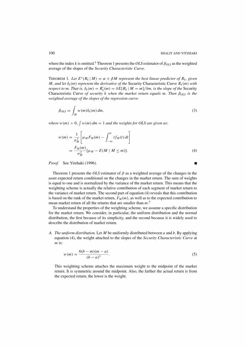
where the index k is omitted.4 Theorem 1 presents the OLS estimator of βOLS as the weightedaverage of the slopes of the Security Characteristic Curve.

THEOREM 1. Let E∗(Rk | M) = α + βM represent the best linear predictor of Rk, givenM, and let δk(m) represent the derivative of the Security Characteristic Curve Rk(m) withrespect to m. That is, δk(m) = R′

k(m) = ∂ E[Rk | M = m]/∂m, is the slope of the SecurityCharacteristic Curve of security k when the market return equals m. Then βOLS is theweighted average of the slopes of the regression curve:

βOLS =∫

Mw(m)δk(m) dm, (3)

where w(m) > 0,∫

w(m) dm = 1 and the weights for OLS are given as:

w(m) = 1

σ 2M

[µM FM(m) −

∫ m

−∞t fM(t) dt

]

= FM(m)

σ 2M

[µM − E(M | M ≤ m)]. (4)

Proof. See Yitzhaki (1996).

Theorem 1 presents the OLS estimator of β as a weighted average of the changes in theasset expected return conditional on the changes in the market return. The sum of weightsis equal to one and is normalized by the variance of the market return. This means that theweighting scheme is actually the relative contribution of each segment of market return tothe variance of market return. The second part of equation (4) reveals that this contributionis based on the rank of the market return, FM(m), as well as to the expected contribution tomean market return of all the returns that are smaller than m.5

To understand the properties of the weighting scheme, we assume a specific distributionfor the market return. We consider, in particular, the uniform distribution and the normaldistribution, the first because of its simplicity, and the second because it is widely used todescribe the distribution of market return.

A. The uniform distribution. Let M be uniformly distributed between a and b. By applyingequation (4), the weight attached to the slopes of the Security Characteristic Curve atm is:

w(m) = 6(b − m)(m − a)

(b − a)3. (5)

This weighting scheme attaches the maximum weight to the midpoint of the marketreturn. It is symmetric around the midpoint. Also, the farther the actual return is fromthe expected return, the lower is the weight.

ESTIMATING BETA 101

B. The normal distribution. Let M be a standard normally distributed variate. Then

w(m) = − 1√2π

∫ m

−∞te−t2/2 dt = 1√

2πe−m2/2. (6)

The weight is identical to the density of the normal distribution. Hence, equal percentilesof the distribution receive equal weights.

These examples reveal that the OLS weighting scheme is determined solely by the distri-bution of the market return and is sensitive to the shape of the distribution. For a flat densityfunction, such as the uniform distribution, the OLS estimator attaches greater weights toobservations that are near the mean of the distribution. When the distribution is normal, anequal number of observations receive exactly the same weight.

Empirical evidence on the distribution of the market rate of return by Fama (1965) and byMantegna and Stanley (1995) indicates fatter tails than expected from a normal distribution.Hence, the weighting scheme of the normal distribution is not a good approximation of theactual weighting scheme in a typical estimation of β. Therefore, instead of identifying thedistribution type and evaluating the weighting scheme for given theoretical distributions, itis useful to establish the weights directly from the sample as follows.

Let us consider a sample of n observations of stock return ri (i = 1, . . . , n) and marketreturn mi . We arrange the observations by ranking them in ascending order of marketreturn. We define �i = mi+1 − mi > 0 as the difference in stock returns, and bi = ri+1−ri

mi+1−mi

(i = 1, . . . , n − 1) as the slope of the line joining two adjacent observations.6

THEOREM 2. Within the sample, the OLS estimator of systematic risk β is the weightedaverage of slopes delineated by adjacent observations. That is,

bOLS =n−1∑i=1

wi bi (7)

where wi > 0,∑

wi = 1.The weights are given by

wi = �i{∑n−1

j=i i(n − j)� j + ∑i−1j=1 j (n − i)� j

}∑n−1

k=1 �k{∑n−1

j=k k(n − j)� j + ∑k−1j=1 j (n − k)� j

} . (8)

Proof. See Yitzhaki (1996).

The components of equation (7) are the slopes bi and the weights wi that depend solely onthe distribution of the independent variable, i.e., the market return. The contribution of eachobservation to the estimator of β consists of (i) the effect of the weighting scheme and (ii) the


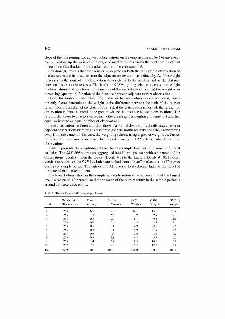
slope of the line joining two adjacent observations on the empirical Security CharacteristicCurve. Adding up the weights of a range of market returns yields the contribution of thatrange of the distribution of the market return to the estimate of β.

Equation (8) reveals that the weights wi depend on both the rank of the observation ofmarket return and its distance from the adjacent observation, as defined by �i . The weightincreases as the rank of the observation draws closer to the median and as the distancebetween observations increases. That is: (i) the OLS weighting scheme attaches more weightto observations that are closer to the median of the market return, and (ii) the weight is anincreasing (quadratic) function of the distance between adjacent market observations.

Under the uniform distribution, the distances between observations are equal, hencethe only factor determining the weight is the difference between the rank of the marketreturn from the median of the distribution. Yet, if the distribution is normal, the farther theobservation is from the median the greater will be the distance between observations. Theresult is that these two factors offset each other, leading to a weighting scheme that attachesequal weights to an equal number of observations.

If the distribution has fatter tails than those of a normal distribution, the distances betweenadjacent observations increase at a faster rate (than the normal distribution rate) as one movesaway from the center. In this case, the weighting scheme assigns greater weights the fartherthe observation is from the median. This property causes the OLS to be sensitive to extremeobservations.

Table 2 presents the weighting scheme for our sample together with some additionalstatistics. The S&P 500 returns are aggregated into 10 groups, each with ten percent of theobservations (deciles), from the lowest (Decile # 1) to the highest (Decile # 10). In otherwords, the returns on the S&P 500 Index are ranked from a “bear” market to a “bull” marketduring the sample period. The entries in Table 2 serve to shed some light on the effect ofthe state of the market on beta.

The lowest observation in the sample is a daily return of −20 percent, and the largestone is a return of +9 percent, so that the range of the market return in the sample period isaround 30 percentage points.

Table 2. The OLS and GMD weighting schemes

Number of Percent Percent OLS GMD GMD(v)Decile Observations of Range of Variance Weights Weights Weights

1 253 66.1 50.3 34.1 15.0 26.42 253 1.3 5.6 7.9 9.9 14.73 253 0.8 2.0 6.4 9.2 11.84 253 0.6 0.6 5.3 8.4 9.15 253 0.5 0.1 4.9 8.0 7.56 253 0.5 0.1 4.9 7.9 6.57 253 0.6 0.6 5.6 8.8 6.28 253 0.9 2.1 6.8 9.9 6.19 253 1.4 6.4 8.3 10.6 5.8

10 252 27.1 32.2 15.7 12.2 6.0

Total 2529 100.0 100.0 100.0 100.0 100.0

ESTIMATING BETA 103

The first column in Table 2 reports the number of observations in each decile. The secondcolumn reports the percentage of the range of the market return used by each decile. Thewider the range of the deciles the lower the density function at that segment of the range.The first decile covers 66 percent of the range while the highest decile covers 27 percent.This implies that the sample distribution has fat tails in that 20 percent of the observationscover 93 percent of the range. Also, there are more extreme observations at the lower tailthan at the upper tail.

The third column presents the contribution of each decile to the variance of the S&P 500return. Formally:

Sn = 10

nσ 2M

∑i∈Dn

[mi − E(m)]2 (9)

where Sn is the contribution of the nth decile to the variance, and Dn represents the nthdecile. That is, the contribution of each observation to the variance is aggregated for eachdecile to obtain the contribution of the decile to the variance of the market.7 The contribu-tion of the lowest decile to the variance is 50 percent, while the highest decile contributes32 percent. Taken together, both deciles contribute 82 percent to the variance of the S&P 500return.

The fifth column shows the contribution of each decile to the OLS weighting scheme,according to equation (8). The slopes of the Security Characteristic Curve are multipliedby this weighting scheme to obtain the betas for the individual firms. The first decile isassigned 34 percent of the weight, while the upper decile is assigned 16 percent. Takentogether, the first and the last decile are responsible for 50 percent of the weights. If theS&P 500 Index return were to be normally distributed, we should find the weight attachedto the two extreme deciles to be 20 percent; If the distribution were to be uniform, then theweight attached to the two extreme deciles should be less than 6 percent. The conclusion isthat the fat tails are responsible for the instability of the OLS estimator of systematic risk.

The remaining entries for the column show that, excluding the extreme deciles, thedistribution is symmetric around the fifth and sixth deciles. Indeed, the weight attachedto the fifth decile is identical to the weight attached to the sixth decile; the weights attachedto the fourth and seventh deciles are almost identical and so on. (The last two columnspresent the weights used for the alternative estimators discussed in Section 3).

Table 2 reveals that one factor contributing to the instability of betas lies in the largerweight allocated to extreme observations. The OLS attaches 50 percent of the weight to20 percent of the observations. The evidence that a relatively high number of DJIA stocksare sensitive to the exclusion of some observations hints that the Security CharacteristicCurve may be non-linear, although this issue is beyond the scope of the current paper sinceCAPM does not require linearity of the Security Characteristic Curve. As is argued in thenext section, portfolio theory and CAPM do not require linearity of the market line northe use of a regression model to compute beta.8 Indeed, under the original CAPM, beta isan ex-ante measure of risk. The use of regression analysis to estimate beta confuses theissue because one has to assume error terms that are uncorrelated with the market portfolio.(Sharpe, 1991).


For our purposes, we distinguish between sensitivity to the upper tail (a “bull” market)and the lower tail (a “bear” market) of the distribution. The greater weight attached to thelower tail of the market distribution can be explained by high levels of risk aversion. Indeed,a risk-averse investor attaches greater weight to the lower tail of the distribution. Therefore,the higher the risk aversion, the greater the weight that should be attached to the lowerportion of the distribution. In the extreme case of a max–min investor, all the weight isattached to the lowest two observations of the market, in order to determine the contributionof the asset to the riskiness of the portfolio (Shalit and Yitzhaki, 1984).

While risk aversion can justify the greater weight assigned to the lower tail, it is not at allclear what would justify the large weight attached to the higher decile of the distribution.On the contrary, risk aversion would indicate that weights be reduced in the face of a bullmarket. Furthermore, in the extreme case of risk neutrality, the weights should not exceedthe weight that is attached when calculating the mean of the distribution. Hence it seemsdifficult to reconcile the quadratic weighting scheme implied by OLS with a weight thatincreases with market returns on the one hand and with risk aversion on the other.

In some sense the number of observations is misleading. Although we have a sample of2529 observations, only 20 percent of these are actually responsible for 50 percent of thecoefficient. Because the weights are not evenly distributed in each decile, the effect is thatwe obtain the sensitivity of beta via the extreme observations.

The issue of the weighting scheme pervades other statistics of the regression such as mis-specification tests and tests based on the error term distribution. Since mis-specificationtests rely on the same weighting scheme, there is no guarantee that such tests do not relyon estimators that stress the non-relevant portions of the distribution. Testing for undueinfluence may therefore be helpful. The effect of an observation takes two forms: (i) itsweight and (ii) the deviation of its slope (defined with adjacent observations) from theaverage slope. If only observations with low weights deviate from the average slope, theinfluence of each observation may be minor, either because of the low weight or becauseof the small deviation of the slope.

We now analyze the implication of economic theory on the estimation procedure ofsystematic risk.

3. Systematic risk

Although beta lost some of its glitter as a result of some empirical tests (e.g., Fama andFrench, 1992), it still maintains its theoretical appeal as a measure of risk. To stress theimportance of systematic risk in financial theory, we argue that only two parameters, theexpected return and the systematic risk, are sufficient in order to capture the entire effect ofthe distribution of the asset’s rate of return on the expected utility of the investor. Systematicrisk is expressed as the covariance between asset return and the marginal utility of wealth.However, the marginal utility of wealth is implicitly assumed. It is the estimation procedureof systematic risk that dictates the implied expected marginal utility of wealth. OLS impliesa quadratic utility which means that the marginal utility of wealth is a linear function ofwealth. This assumption of linearity is responsible for the sensitivity of beta to fat tails.

ESTIMATING BETA 105

The CAPM relating beta to expected return was originally derived by assuming mean-variance efficiency of portfolios.9 Afterward, following the Rothschild and Stiglitz (1970)increasing risk model, Merton (1982, 1990) proved the CAPM relationship for all risk-averseinvestors by postulating efficient portfolios, in the sense that investors maximize expectedutility. Portfolio efficiency, whether in mean-variance or expected utility, is the conditionnecessary to derive CAPMs. As Roll (1977) noted however, market efficiency is itself thestipulation that prevents a valid test of asset pricing theory.

We alleviate this problem by showing how the expected utility or disutility produced by asmall change in the holdings of one asset in the portfolio can be captured in terms of expectedreturn and systematic risk. This result is valid for all expected utility maximizers, and hencedepends neither upon the quadraticity of preferences nor the distribution of returns.

We do not assume that investors actually succeed in maximizing expected utility, thusdeparting from Merton (1982, 1990). Although the intended goal is to maximize expectedutility, it may not be achieved because of transaction costs, a lack of perfect information,constant changing environments, or other commitments. Hence, the definition of systematicrisk does not depend on whether investors are able to maximize the expected utility since itis sufficient to assume that they intend to do so.

Consider an expected utility maximizing investor who holds a mixed portfolio of riskyand safe assets. The investor’s goal is represented by the maximization problem:

maxα1,...,αn

E[U (M)]

s.t. M = M0

[y +

n∑i=1

αi Ri

](10)

n∑i=1

αi = 1 and M0 ≡ 1,

where E[U (M)] is expected utility; U is a continuous, monotonically increasing concavefunction, M0 is a given initial wealth assumed to be 1 without loss of generality; αi andRi are, respectively, the share of M invested in asset i and the returns on asset i ; and y isthe return on some other income, either deterministic or stochastic that can be attributed tolabor or human capital.

The investor holds a given portfolio {α0}, whose shares are α0i , i = 1, . . . , n. Note that

the only requirement on α0 is that it is held by the investor. Assume the investor wants tochange the holdings of asset k in the portfolio. The effect of increasing α0

k on expectedutility is given by:

∂ E[U (M)]

∂αk= E[U ′(M)Rk] − λ, (11)

where λ is the Lagrange multiplier associated with the portfolio constraint. By addingand subtracting E[U ′(M)]µk , where µk is the expected return on asset k, we can rewrite


equation (2) as:

∂ E[U (M)]

∂αk= E[U ′(M)]µk + cov[U ′(M), Rk] − λ. (12)

Our purpose here is to compare between assets. Hence, all factors that are equal for allassets can be ignored. Equation (12) expresses the effect of a marginal increase in asset kon expected utility as a function of the expected return on asset k, and the asset’s systematicrisk, defined as the covariance between marginal utility of wealth and the return on asset k.

Assuming a specific utility function enables us to obtain an explicit expression for syste-matic risk. For example, a quadratic utility function defined on wealth leads to the conven-tional beta. Formally, let us denote U (M) = A + BM + 0.5 CM2; then cov[U ′(M), Rk] =βkσ

2M , where βk = βOLS = cov(Rk, M)/cov(M, M) is the OLS regression coefficient of Rk

on M . If the utility function is defined in terms of the rate of return on the portfolio ratherthan the level of wealth, the standard expression for systematic risk is produced.

If investors identify risk with another index of variability, such as the semivariance or theGini’s Mean Difference (GMD), alternative expressions for beta may be obtained (Shalit andYitzhaki, 1984). In the case of GMD, βk = cov[Rk, F(M)]/cov[M, F(M)] where F(M)

is the cumulative probability distribution of investors’ wealth. The implied utility functionin this case can be traced to a special case of Yaari’s (1987) dual approach to risk aversion.

An alternative to the assumption, explicit or implicit, of a specific utility function is toconsider a set of utility functions that comply with second degree stochastic dominance(SSD), where the set of eligible functions is composed of all utility functions with U ′( ) > 0and U ′′( ) < 0.10 Then one can summarize the effect of an increase in the share of an asseton all possible legitimate utility functions by a curve instead of a single parameter as in thecase of specific utilities.

Under SSD, the effect of increasing α0k on expected utility is captured by the following

Theorem:

THEOREM 3. A necessary and sufficient condition for a small increase in asset k to increaseexpected utility for all functions with U ′ > 0 and U ′′ < 0 given portfolio M is

ACCMk (p) =

∫ m

−∞Rk(t) fM(t) dt ≥ 0 for all m, where p =

∫ m

−∞fM(t) dt, (13)

where ACC stands for the absolute concentration curve and Rk( ) is the conditional expectedreturn on asset k given a portfolio return.

Proof. See Shalit and Yitzhaki (1994), where the theorem is proved for an increase in theshare of one asset subject to a decrease in the share of another asset.

The ACC of asset k sums up the conditional expected returns on asset k, each weightedby the probability of the portfolio M = m. The probability p is that the portfolio return isat most m. Hence for a given probability p, the ACC is the cumulative expected return onasset k, subject to a portfolio return of, at most, m.

ESTIMATING BETA 107

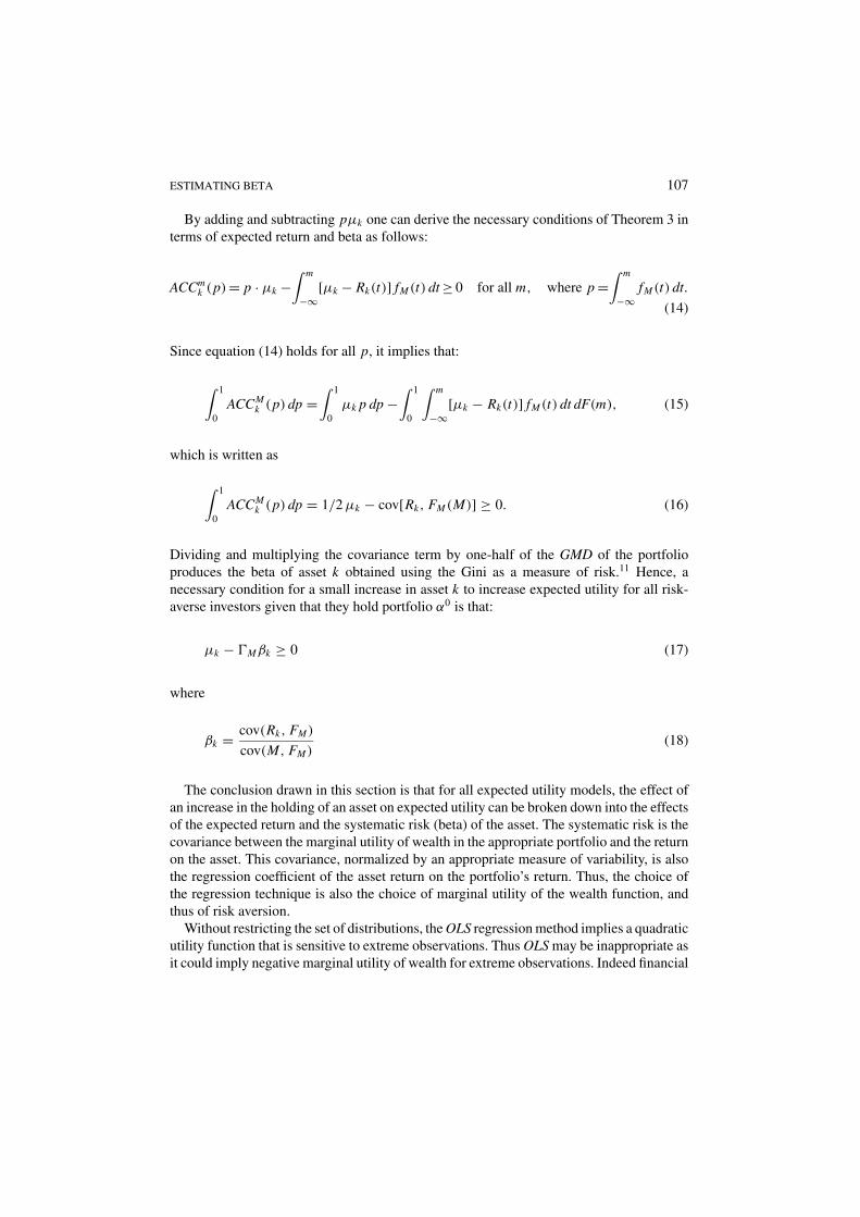
By adding and subtracting pµk one can derive the necessary conditions of Theorem 3 interms of expected return and beta as follows:

ACCmk (p) = p · µk −

∫ m

−∞[µk − Rk(t)] fM(t) dt ≥ 0 for all m, where p =

∫ m

−∞fM(t) dt.

(14)

Since equation (14) holds for all p, it implies that:

∫ 1

0ACCM

k (p) dp =∫ 1

0µk p dp −

∫ 1

0

∫ m

−∞[µk − Rk(t)] fM(t) dt dF(m), (15)

which is written as

∫ 1

0ACCM

k (p) dp = 1/2 µk − cov[Rk, FM(M)] ≥ 0. (16)

Dividing and multiplying the covariance term by one-half of the GMD of the portfolioproduces the beta of asset k obtained using the Gini as a measure of risk.11 Hence, anecessary condition for a small increase in asset k to increase expected utility for all risk-averse investors given that they hold portfolio α0 is that:

µk − �Mβk ≥ 0 (17)

where

βk = cov(Rk, FM)

cov(M, FM)(18)

The conclusion drawn in this section is that for all expected utility models, the effect ofan increase in the holding of an asset on expected utility can be broken down into the effectsof the expected return and the systematic risk (beta) of the asset. The systematic risk is thecovariance between the marginal utility of wealth in the appropriate portfolio and the returnon the asset. This covariance, normalized by an appropriate measure of variability, is alsothe regression coefficient of the asset return on the portfolio’s return. Thus, the choice ofthe regression technique is also the choice of marginal utility of the wealth function, andthus of risk aversion.

Without restricting the set of distributions, the OLS regression method implies a quadraticutility function that is sensitive to extreme observations. Thus OLS may be inappropriate asit could imply negative marginal utility of wealth for extreme observations. Indeed financial


theory under risk aversion assumes a declining marginal utility of wealth. Furthermore, thehigher the degree of risk aversion, the faster marginal utility declines with wealth. Thisimplies that risk-averse investors attribute less weights for variability when market returnsare high than when market returns are low. On the other hand, as seen from equation (4),since the OLS weighting scheme is symmetric with respect to the median of market returns,OLS will be incompatible with risk aversion and declining marginal utility of wealth.

The bottom line of our argument is that investors’ risk aversion as it appears in CAPMmust be the same risk aversion used when estimating systematic risk. In the next section, wepropose an alternative estimation method of the market line that will be both more robustthan the OLS, and will at the same time better reflect the risk aversion of the investors.

4. Alternative estimators for beta

Theorems 1 and 2 provide a formal explanation for the well-known observation that OLSestimators are sensitive to outliers. A common solution to this problem is to remove extremeobservations from the sample. The inconsistency in this procedure is inherent. On the onehand, outliers receive extremely high weights. On the other hand, when they appear to have astrong effect on the estimate, they are arbitrarily deleted from the sample along with therelevant information they carry.

The OLS estimator can be interpreted as a weighted average of slopes. As we obviouslydo not want to change the slopes, the solution must rely on changing the weighting schemeand making it compatible with risk averse behavior. The weighting scheme depends upon(i) the rank of each observation and (ii) the difference (in terms of the independent variable)between each observation and the one adjacent. In OLS this difference is raised to the secondpower, thus exacerbating its effect.12

An alternative strategy is one that yields a weighting scheme that is consistent with one’sperception of risk aversion. Therefore, one should use indices of variability that are lesssensitive to extreme high rates of market return and that imply regression slope estimatorswith low weights to extreme high observations. Such properties exist in the Gini estimators.

As far as we know, Gini’s statistics were first applied as measures of dispersion in financialdata by Fisher and Lorie (1970) who justify their use “. . . because many of the distribut-ions . . . depart greatly from normality. For such distributions, the standard deviation of evena large sample may not give a very meaningful indication of the dispersion of the population.Gini’s mean difference and coefficient of concentration are nonparametric measures and areinvulnerable to this consequence of departure from normality . . . Gini’s mean differencediffers from the mean deviation by giving greater weight to extreme observations, thustaking care of a frequently made criticism of the mean deviation” (1970, p. 104).

The extended Gini is a family of variability measures that was applied by Yitzhaki (1983)to develop necessary conditions for stochastic dominance. It was used by Shalit and Yitzhaki(1984) to develop the Mean-Gini CAPM which is similar to MV-CAPM in its properties but,unlike MV, is consistent with expected utility for any concave function or any probabilitydistribution. Even if one wants to rely on MV-CAPM as the theoretical basis for developingsystematic risk, it may be helpful to use the beta Gini estimator as a robust estimate of

ESTIMATING BETA 109

beta.13 That is to say, one can recommend the Gini beta on its own merits or as a robustestimator for the MV beta.

The extended Gini regression coefficient (EGRC) is a ratio based on the extended Ginivariability index. The denominator denotes the market extended Gini index and the numer-ator the extended Gini covariance of the stock return with the market return.14 EGRC isdefined as:15

β(v) = cov(R, [1 − FM(M)]v−1)

cov(M, [1 − FM(M)]v−1)v > 0, v �= 1 (19)

where v is a parameter determined by the investigator to reflect the investigator’s perceptionof risk aversion in the market.16 If v = 1, the investigator assumes a risk-neutral market.The higher the v the more risk-averse is the market. In the extreme case (v = ∞), the marketconcerns itself only with huge crashes (which is exhibited by max–min behavior). The range0 ≤ v < 1 reflects risk-loving behavior with v → 0 showing a max–max strategy; i.e.,the market considers only the day with the highest return as the decision statistic. Anotherinterpretation of v is to view as a parameter in a specific set of utility functions belonging tothe set of utility functions that comply with Yaari’s (1987) dual approach to decision underrisk.

The weighting scheme of the estimator for β(v) is determined by the parameter v and bythe distribution of the market return. By determining v, the investigator introduces individualperception of risk aversion into the estimation procedure.

THEOREM 4. The extended Gini estimators of the regression coefficient have the followingproperties:

(a) In the population the parameters are the weighted averages of the slopes of the SecurityCharacteristic Curve:

β(v) =∫

V (m, v)δ(m) dm, (20)

with V (m, v) > 0 and∫

V (m, v) dm = 1, where

V (m, v) = [1 − FM(m)] − [1 − FM(m)]v∫ ∞−∞{[1 − FM(t)] − [1 − FM(t)]v} dt

. (21)

(b) In the sample, all estimators are weighted averages of slopes defined by pairs ofadjacent observations:

b(v) =n−1∑i=1

Vi (v)bi , (22)


where

bi = ri+1 − ri

mi+1 − mi(i = 1, . . . , n − 1); Vi > 0, �Vi = 1,

and

Vi (v) = [nv−1(n − i) − (n − i)v] �i∑n−1k=1[nv−1(n − k) − (n − k)v] �k

. (23)

(c) The estimators b(v) are ratios of U-statistics. Hence, they are consistent estimatorsof β(v). For large samples, the distribution of the estimators converges to a normaldistribution. Furthermore, for integer v, the estimators b(v) are unbiased and have aminimum variance among all unbiased estimators.

(d) Suppose that E(Y | X) = α + β X and var(Y | X) = σ 2 < ∞. Then all extended Giniestimators are consistent estimators of β.

Proof. See Yitzhaki (1996) and Schechtman and Yitzhaki (1998).

Properties (a) and (b) show that all EGRC(v) are weighted averages of the slopes definedby adjacent sample points. The differences among the estimators are in the weightingschemes. Property (d) of Theorem 4 enables the use of EGRC as an estimator for MV-beta.

To estimate EGRC it is not necessary to assume a linear relationship. All that is requiredis to assume a regression curve and an interest in estimating a weighted average of thecurve slopes. The weights are determined by two elements: The first is the perception ofrisk aversion and the second is the statistical property of the estimate that depends on thedistribution of the market return.

For a given v, we can ignore the denominator as a normalizing factor and consider thenumerator as a function of the value p = i/n provided by the cumulative distribution:

w(p) = c(v)[(1 − p) − (1 − p)v], (24)

where c is a function of v. By looking at the derivatives of w with respect to the cumulativedistribution p, we can trace the properties of the weighting scheme:

∂w

∂p= ∂w[FM(m)]/∂m

∂ FM(m)/∂m= c(v)[v(1 − p)v−1 − 1]

and

∂2w

∂p2= c(v)v(v − 1)(1 − p)v−2.

For v > 1, i.e., for a risk-averse investigator, the weighting scheme increases for low val-ues of p, reaches a maximum, and then declines. If v < 1, i.e., for a risk-loving investigator,the weighting scheme increases with p.17

ESTIMATING BETA 111

If v = 2, the denominator of equation (19) is one-half the GMD, while the numerator isthe Gini covariance. The weighting scheme is symmetric in p. The closer the observationis to the median, the greater is its weight.

The GMD weighting scheme is similar to the OLS weighting scheme, except that the OLSweighting scheme uses quadratic distances between observations, while the GMD weightingscheme uses absolute differences. If the distance between observations of the market returnis constant, such as in the uniform distribution, the weighting scheme of GMD is identical tothat of OLS. If the distribution of the market return is normal, GMD attaches higher weightsto the center of the distribution than OLS does. That is, while the OLS attaches equal weightsto equal numbers of observations, the GMD attaches higher weights to the middle of thedistribution. In general, since the denominator in equation (19) is the extended Gini, it canbe shown that the GMD (and the extended Gini) weighting schemes attribute to each decileof the distribution the contribution of that decile to the GMD (or the extended Gini).

The weighting scheme of the GMD beta is shown in the fifth column of Table 2. It can beseen that the GMD attaches only 15 percent of the weight to the lowest decile and 12 percentto the highest decile. Thus, the use of the Gini reduces the weight attached to the two extremedeciles of the market return from 50 percent under OLS to 27 percent under GMD.

The effect of changing v on the weighting scheme is more complex, since both thenumerator and the denominator are affected. If v > 1, that is, if risk aversion is considered,higher weights are given to the lower segments of the market distribution returns.

The weighting scheme for each v can be calculated numerically. The last column ofTable 2 presents the weighting scheme for v = 5. By raising v from 2 to 5, the weightassigned to the lowest decile increases to 26 percent, while the weight assigned to thehighest decile decreases from 12 to 6 percent. This approach enables the investigator tocontrol the weighting scheme and to adjust it to the market risk aversion.

Table 3 presents the sensitivity of beta derived under various approaches to the deletionof the top four and the bottom four market return observations. Since the standard errorof each estimate is derived under different assumptions, the estimates are not comparable.Therefore, Table 3 reports the absolute deviation of beta in each method in percentage pointsof the estimate. The first four columns report the effect of deleting the top four observations.In this case, the βOLS of more than six firms (20 percent of the sample) changes by more than

Table 3. Percentage deviation of beta OLS and beta Gini

βOLS βv=2 βv=4 βv=6 βOLS βv=2 βv=4 βv=6

Number of omitted data 4 4 4 4 8 8 8 8More than 10% deviation 0 0 0 0 8 0 0 05–10% deviation 2 0 0 0 10 0 0 13.0–5.0% deviation 4 0 0 0 3 2 1 02.0–3.0 8 2 0 0 2 4 5 81.0–2.0 9 7 3 0 3 10 11 12Less than 1.0 7 21 27 30 4 14 13 9Total 30 30 30 30 30 30 30 30Maximum deviation 7.7 2.3 1.2 1.0 12.7 3.1 2.4 2.5Minimum deviation −4.2 −1.5 −0.8 −0.6 −15.2 −4.0 −4.8 −5.7


3 percentage points, but none of the Gini betas (with v = 2, 4, 6) change by this magnitude.The OLS betas of an additional eight firms change by more than 2 percent while only theGMD betas of two stocks have changed by this magnitude. As expected, the higher the vthe less sensitive is the estimate of beta to the firm performance in extreme high marketreturns. To illustrate, note that for v = 6 all betas have changed by less than 1 percent.

The second four columns report the sensitivity of the estimates when both the top andbottom four observations are omitted. Under OLS, the betas of more than eight firms changeby more than 10 percent, while the Gini betas in no case change by that magnitude. It alsocan be seen that increasing v increases the sensitivity of beta because of the increase in theweight given to bottom observations. Nevertheless, the Gini method continues to be morerobust than OLS. If one continues to increase v, however, this property disappears.

The extended Gini approach offers an infinite number of alternative estimators. Twoimmediate questions arise: should the Gini method be used as a substitute for OLS estimationand, if so which v should be chosen. The answer is not clear-cut. On the one hand, itdepends on the degree of confidence one has about the market’s risk aversion and, on theother hand, on the curvature of the empirical Security Characteristic Curve. If the SecurityCharacteristic Curve is linear, it does not matter which method is used. If the slopes of thecurve differ, i.e., if the relationship between the firm and the market is not linear, the methodused is important. In this sense, EGRC offers a statistical test on whether incorporating theparameter of risk aversion in the estimation is important. As shown by Gregory-Allen andShalit (1999) statistically testing the equality of various β(v) is actually a test on the linearityof the regression curve, and therefore can determine whether v is significantly important.

Ignoring risk aversion and assuming the validity of MV, OLS is the most efficient esti-mator. If the model is linear, using a Gini-based estimator will result in loss of efficiency.The larger the sample size however the less important is the efficiency loss.

If the Security Characteristic Curve is not linear, and if the stock market exhibits greatvolatility, OLS may lead to estimating wrong coefficients. Hence MV-CAPM may fail, notbecause of wrong assumptions but rather because of the estimation procedure. Furtherresearch would be fruitful in this area.

The Gini method does not need to specify the curvature of the Security CharacteristicCurve. It provides a weighted average of the slopes where the weights are determined byrisk aversion (theory) and statistical (curvature) considerations.

5. Further research and conclusion

The question remains as to how a Gini-based model can serve as a basis for testing CAPM.This is a complex issue because of the infinite number of risk aversion parameters v. Indeedone should ask what is the proper v to be used? With MV, risk aversion differentiation amongagents vanishes in market equilibrium because of the separation theorem. Differences inrisk aversion among investors only materialize in the various combinations of the risklessasset and the market portfolio. This is not the case with MEG betas, where risk aversionconsideration appears in the estimation of systematic risk. This issue was also studied byLevy (1978) within MV. By considering investors who hold portfolios of stocks whose

ESTIMATING BETA 113

number is smaller than the number of stocks in the market, Levy shows that several MVbetas for the same stock co-exist in equilibrium.

In the same spirit, we posit that different betas generated from various risk aversioncoefficients can coexist in equilibrium in the same market. The challenge would be toestablish the theoretical foundations for such a model. In the meantime we are compelled touse a market equilibrium with a unique Gini beta based on one coefficient of risk aversion,v. For that purpose, one approach is to estimate v most likely held by investors by comparingthe mean-Gini efficient sets with the market portfolio, as Shalit and Yitzhaki (1989) havedone.

In all expected utility models, the systematic risk of an asset can be presented as a functionof a covariance between marginal utility of wealth and the return on the asset. In estimatingbeta by OLS, the marginal utility is represented by a linear function of the market return,implying that the utility function is quadratic. Together with the fat tails of the marketdistribution, this leads to an unwarranted sensitivity of the beta and to contradiction of theassumption of positive marginal utility of wealth. Further research is needed to verify thatthe cross-section estimating CAPM will not yield negative marginal utility of wealth. TheGMD beta does not suffer from this problem and offers an alternative and robust estimationmethod of systematic risk.

Appendix

Table A1.

(I) Beta for (II) Beta w/o (III) Beta w/o (I)–(II)/ (I)–(III)/Firm All Data 4 Top Data 8 Data Std Err Std Err

ALLIED SIGNAL 1.0503 1.0287 0.8909 0.7142 5.2819(0.030) (0.029) (0.033)

AMERICAN EXPRESS 1.3902 1.3792 1.3843 0.3528 0.1879(0.031) (0.032) (0.037)

AT&T 1.0600 1.0585 1.0665 0.0641 −0.2766(0.023) (0.024) (0.027)

BANK AMERICA 1.1381 1.1124 1.0490 0.6372 2.2085(0.040) (0.041) (0.047)

CATERPILLAR 0.9912 1.0038 0.9817 −0.4118 0.3115(0.030) (0.031) (0.035)

CHEVRON 0.8362 0.8598 0.8339 −0.9413 0.0906(0.025) (0.026) (0.029)

COCA-COLA 1.2159 1.1851 1.1823 1.3753 1.4983(0.022) (0.022) (0.026)

DEERE 0.9127 0.9293 0.9278 −0.5025 −0.4555(0.033) (0.034) (0.038)

DISNEY 1.1811 1.1528 1.0938 0.9389 2.8916(0.030) 0.0309 0.0351

(continued)


Table A1. (Continued)

(I) Beta for (II) Beta w/o (III) Beta w/o (I)–(II)/ (I)–(III)/Firm All Data 4 Top Data 8 Data Std Err Std Err

DOW CHEMICAL 1.0828 1.0994 1.0999 −0.6600 −0.6807(0.025) (0.026) (0.029)

DU PONT 1.0101 1.0400 1.0731 −1.3735 −2.8881(0.022) (0.022) (0.025)

KODAK 1.0841 1.0510 0.9529 1.1807 4.6814(0.028) (0.028) (0.031)

EXXON 0.9451 0.9221 0.8680 1.0975 3.6807(0.021) (0.021) (0.024)

GE 1.1569 1.1595 1.2324 −0.1428 −4.1507(0.018) (0.019) (0.021)

GM 1.0557 1.0661 1.0958 −0.3834 −1.4772(0.027) (0.028) (0.031)

GOODYEAR 1.0246 1.0053 0.9129 0.5781 3.3347(0.034) (0.034) (0.039)

IBM 0.9478 0.9535 0.9207 −0.2458 1.1885(0.023) (0.023) (0.027)

INT’L PAPER 1.0966 1.1137 1.0435 −0.6685 2.0753(0.026) (0.026) (0.029)

J&J 1.0894 1.1059 1.1555 −0.6804 −2.7193(0.024) (0.025) (0.028)

MCDONALDS 1.0039 0.9956 1.0343 0.3434 −1.2695(0.024) (0.025) (0.028)

MERCK 0.9263 0.9419 1.0263 −0.6752 −4.3308(0.023) (0.023) (0.027)

MMM 1.0127 1.0223 0.9599 −0.5084 2.8060(0.019) (0.019) (0.022)

MOBIL 0.9262 0.8874 0.8170 1.5448 4.3431(0.025) (0.026) (0.029)

JP MORGAN 1.1958 1.1581 1.0789 1.3914 4.3172(0.027) (0.026) (0.030)

PHILIP MORRIS 0.9850 0.9965 1.0738 −0.4706 −3.6300(0.024) (0.025) (0.028)

PROCTER & GAMBLE 1.0508 1.0278 0.9900 1.0518 2.7725(0.022) (0.021) (0.024)

SEARS 1.1535 1.1383 1.1324 0.5524 0.7697(0.027) (0.028) (0.032)

UNION CARBIDE 0.8995 0.9295 1.0091 −0.8195 −2.9952(0.037) (0.036) (0.041)

UNITED TECH 0.8385 0.9028 0.9448 −2.3928 −3.9564(0.027) (0.027) (0.031)

WOOLWORTH 0.9460 0.9951 1.0494 −1.5971 −3.3616(0.031) (0.031) (0.036)

ESTIMATING BETA 115

Table A2.

Portfolio (I) Beta for (II) Beta w/o (III) Beta w/o (I)–(II) (I)–(III)Number All Data 4 Highest Data 8 Data Over Std Err Over Std Err

1 0.4607 0.4598 0.4698 0.06000 −0.59761(0.015) (0.016) (0.018)

2 0.5672 0.5639 0.5755 0.28295 −0.70939(0.012) (0.012) (0.014)

3 0.6325 0.6327 0.6366 −0.01948 −0.32324(0.013) (0.013) (0.015)

4 0.7208 0.7072 0.6785 1.13498 3.52226(0.012) (0.012) (0.014)

5 0.8269 0.8460 0.8080 −1.30485 1.28871(0.015) (0.015) (0.017)

6 0.8776 0.8825 0.8910 −0.35783 −0.97399(0.014) (0.014) (0.016)

7 0.9135 0.9391 0.9649 −1.56990 −3.15718(0.016) (0.016) (0.018)

8 0.9365 0.9336 0.9348 0.22552 0.13190(0.013) (0.013) (0.015)

9 0.9565 0.9564 0.9265 −0.06964 2.55339(0.011) (0.011) (0.013)

10 0.9807 1.0005 0.9703 −1.16677 0.61295(0.017) (0.017) (0.019)

11 1.0073 1.0226 1.0240 −1.30895 −1.42779(0.012) (0.012) (0.013)

12 1.0423 1.0333 0.9936 0.69029 3.74751(0.013) (0.013) (0.014)

13 1.0684 1.0672 1.0406 0.10475 2.35012(0.012) (0.012) (0.013)

14 1.0893 1.1145 1.1143 −1.49423 −1.48475(0.017) (0.017) (0.020)

15 1.1053 1.1189 1.1313 −0.99743 −1.90759(0.013) (0.014) (0.016)

16 1.1257 1.1194 1.0619 0.37876 3.81387(0.017) (0.017) (0.019)

17 1.1548 1.1520 1.1274 0.12952 1.24226(0.022) (0.022) (0.026)

18 1.2009 1.1973 1.2176 0.27806 −1.30098(0.013) (0.013) (0.015)

19 1.2576 1.2801 1.3176 −1.32833 −3.55031(0.017) (0.017) (0.020)

20 1.3846 1.4081 1.4867 −1.00132 −4.35127(0.023) (0.024) (0.027)


Acknowledgments

Our thanks to Eugene Kandel, Eli Elyasiani, and one anonymous referee for their helpfulcomments and suggestions.

Notes

1. Recently followed by Mantegna and Stanley (1995), Mandelbrot (1963) and Fama (1965) supply the earlyevidence that the distribution of stock returns is characterized by fat tails relative to a normal distribution. Seealso Chan and Lakonishok (1992) for an excellent survey of the literature on non-robustness in estimatingbetas.

2. See the results in Brown and Warner (1985) and Fama (1965) that daily returns depart from normality morethan monthly returns.

3. The estimates for betas are presented in the Appendix.4. The index k will be omitted throughout the paper to avoid confusion.5. In the sample, the cumulative distribution FM (m) is estimated by the rank of m.6. To simplify the presentation we assume without loss of generality that �i > 0. Otherwise, we would need

to aggregate all observations with the same market return m, a procedure that complicates the presentationwithout adding insight.

7. Note that the numerators of both equations (9) and (8) present alternative decompositions of the variance ofthe market return. However, while equation (9) presents it the usual way by writing the variance as squareddeviations from the mean, equation (8) presents it using the change in market return, �i , instead of the marketreturn, m.

8. Roll’s (1977) critique is mainly concerned with the linearity of the relationship between beta and expectedreturn, which is beyond the scope of this paper.

9. The CAPM was first derived by Sharpe (1964), Lintner (1965), and Mossin (1966). Merton (1972) providesa rigorous mathematical analysis of the efficient frontier which also appears in Roll’s (1977) widely citedpaper.

10. For the definition of the SSD criterion see Hadar and Russell (1969) and Hanoch and Levy (1969). See Levy(1992) for a thorough survey of the methodology.

11. The GMD of portfolio M is defined as �M = 2 cov(M, FM ).12. The quadratic differences can be attributed to calculating the variance.13. See Carroll, Thistle and Wei (1992) for a discussion of the robustness properties of the beta Gini estimator.14. For simplicity of exposition only the parameters are presented. The estimators take the same form as the

parameters, except that sample statistics are used instead of population parameters, and the empirical distri-bution is used instead of the cumulative distribution. See Schechtman and Yitzhaki (1998) for an investigationof the large sample properties of the estimators in a multiple regression framework; Olkin and Yitzhaki (1992)for an investigation of large sample properties of the regression based on the GMD, and Yitzhaki (1991) fora derivation of the standard error of the estimators.)

15. This estimator can be interpreted within the framework of OLS regression as an instrumental variable estimatorwith instrument [1 − FM (M)]v. This provides a solution in the presence of errors-in-variables problems,Durbin (1954).

16. Two different questions arise when a measure of variability is used to represent risk. The first is how riskaversion is defined, and the second is how much expected return one is ready to sacrifice in order to reduceexposure to risk. The first question is answered by the choice of the index of variability used (variance,semivariance, extended Gini), while the answer to the second question depends on the curvature of theefficient frontier of risk (measured by the appropriate index) as compared to expected return.

17. The risk aversion implied by the extended Gini coefficient can be described by a specific case. Considerthe utility function: U [µ, �(v)] = µ − �(v) where v is equal to an integer and �(v) is the extended Ginicoefficient. Then it can be shown that µ − �(v) = E[min{M1, M2, . . . , Mv}], where Mi are i. i. d. variables

ESTIMATING BETA 117

(Yitzhaki, 1983). That is, the investor maximizes the expected value of the minimum of v random draws fromthe market return. Hence, when v equals one the investor does not care about risk; when v converges to infinitythe investor behaves as if the worst case scenario will certainly occur. A max–max investor behaves as if thebest realization is always obtained.

References

Amihud, Y., B. J. Christensen and H. Mendelson. Further Evidence on the Risk-Return Relationship. Workingpaper, New York University, 1992.

Brown, S. J. and J. B. Warner, “Using Daily Stock Returns.” Journal of Financial Economics 14, 3–31, (1985).Carroll, C., P. D. Thistle and K. C. John Wei, “The Robustness of Risk-Return Nonlinearities to the Normality

Assumption.” Journal of Financial and Quantitative Analysis 27(3), 419–435, (1992).Chan, L. K. C. and J. Lakonishok, “Robust Measurement of Beta Risk.” Journal of Financial and Quantitative

Analysis 27, 265–282, (1992).Durbin, J., “Errors in Variables.” International Statistical Review 22, 23–32, (1954).Fama, E., “The Behavior of Stock Prices.” Journal of Business 38, 34–105, (1965).Fama, E. F. and K. R. French, “The Cross-Section of Expected Stock Returns.” Journal of Finance 47, 427–465,

(1992).Fama, E. F. and K. R. French, “Common Risk Factors in the Returns on Stocks and Bonds.” Journal of Financial

Economics 33, 3–56, (1993).Fama, E. F. and K. R. French, “Size and Book-to-Market Factors in Earnings and Returns.” Journal of Finance

50, 131–155, (1995).Fama, E. F. and K. R. French, “Industry Costs of Equity.” Journal of Financial Economics 44, 153–193, (1997).Fama, E. F. and J. D. MacBeth, “Risk, Return, and Equilibrium: Empirical Tests.” Journal of Political Economy

81, 607–636, (1973).Fisher, L. and J. H. Lorie, “Some Studies of Variability of Returns on Investments in Common Stocks.” Journal

of Business 43, 99–134, (1970).Gibbons, M. R., “Multivariate Tests of Financial Models: A New Approach.” Journal of Financial Economics 10,

3–27, (1982).Gregory-Allen, R. B. and H. Shalit, “The Estimation of Systematic Risk under Differentiated Risk Aversion: A

Mean-Extended Gini Approach.” Review of Quantitative Finance and Accounting 12, 135–157, (1999).Hadar, J. and W. R. Russell, “Rules for Ordering Uncertain Prospects.” American Economic Review 59, 25–34,

(1969).Hanoch, G. and H. Levy, “The Efficiency Analysis of Choices Involving Risk.” Review of Economic Studies 36,

335–346, (1969).Jagannathan, R. and Z. Wang, “The Conditional CAPM and the Cross-Section of Expected Returns.” Journal of

Finance 51, 3–53, (1996).Kandel, S. and R. F. Stambaugh, “Portfolio Inefficiency and the Cross-Section of Expected Returns.” Journal of

Finance 50, 157–184, (1995).Knez, P. J. and M. J. Ready, “On the Robustness of Size and Book-to-Market in Cross-Sectional Regressions.”

Journal of Finance 52, 1355–1382, (1997).Levhari, D. and H. Levy, “The Capital Asset Pricing Model and the Investment Horizon.” The Review of Economics

and Statistics 59, 92–104, (1977).Levy, H., “Equilibrium in an Imperfect Market: A Constraint on the Number of Securities in the Portfolio.”

American Economic Review 68, 643–658, (1978).Levy, H., “Stochastic Dominance and Expected Utility: Survey and Analysis.” Management Science 38, 555–593,

(1992).Levy, H., “Risk and Return: An Experimental Analysis.” International Economic Review 38(1), 119–149, (1997).Levy, H. and G. Schwarz, “Correlation and the Time Interval over which Variables are Measured.” Journal of

Econometrics 76, 341–350, (1997).


Lintner, J., “The Valuation of Risk Assets and the Selection of Risky Investments in Stock Portfolios and CapitalBudgets.” Review of Economics and Statistics 47, 13–37, (1965).

MacKinlay, A. C. and M. P. Richardson, “Using Generalized Methods of Moments to Test Mean-Variance Effi-ciency.” Journal of Finance 46, 511–527, (1991).

Mandelbrot, B., “The Variation of Certain Speculative Prices.” Journal of Business 36, 394–419, (1963).Mantegna, R. N. and H. E. Stanley, “Scaling Behaviour in the Dynamics of an Economic Index.” Nature 376,

46–49, (1995).Merton, R. C., “An Analytic Derivation of the Efficient Portfolio Frontier.” Journal of Financial and Quantitative

Analysis 7, 1851–1872, (1972).Merton, R. C., “On the Microeconomic Theory of Investment under Uncertainty,” in K. J. Arrow and M. D.

Intrilligator (Eds.), Handbook of Mathematical Economics Vol. II, Amsterdam: North-Holland, 1982.Merton, R. C., Continuous Finance, Cambridge, UK: Blackwell, 1990.Mossin, J., “Equilibrium in a Capital Market.” Econometrica 34, 768–783, (1966).Olkin, I. and S. Yitzhaki, “Gini Regression Analysis.” International Statistical Review 60, 185–196, (1992).Roll, R., “A Critique of the Asset Pricing Theory’s Test: Part I, On Past and Potential Testability of the Theory.”

Journal of Financial Economics 4, 129–176, (1977).Rothschild, M. and J. E. Stiglitz, “Increasing Risk I: A Definition.” Journal of Economic Theory 3, 66–84, (1970).Schechtman, E. and S. Yitzhaki, Asymmetric Gini Regression. Working paper, Hebrew University of Jerusalem,

Department of Economics, 1998.Shalit, H. and S. Yitzhaki, “Mean-Gini, Portfolio Theory and the Pricing of Risky Assets.” Journal of Finance

39(5), 1449–1468, (1984).Shalit, H. and S. Yitzhaki, “Evaluating the Mean-Gini Approach to Portfolio Selection.” International Journal of

Finance 1(2), 15–31, (1989).Shalit, H. and S. Yitzhaki, “Marginal Conditional Stochastic Dominance.” Management Science 40, 670–674,

(1994).Shanken, J., “On the Estimation of Beta-Pricing Models.” Review of Financial Studies 5, 1–33, (1992).Sharpe, W. F., “Capital Asset Prices: A Theory of Market Equilibrium under Conditions of Risk.” Journal of

Finance 19, 425–442, (1964).Sharpe, W. F., Investments, second edition. Englewood Cliffs, NJ: Prentice Hall, 1981.Sharpe, W. F., “Capital Asset Prices with and without Negative Holdings.” Journal of Finance 46, 489–509, (1991).Stambaugh, R. F., “On the Exclusion of Assets from Tests of the Two-Parameter Model: A Sensitivity Analysis.”

Journal of Financial Economics 10, 237–268, (1982).Yaari, M. E., “The Dual Theory of Choice Under Risk.” Econometrica 55, 95–115, (1987).Yitzhaki, S., “Stochastic Dominance, Mean-Variance, and Gini’s Mean Difference.” American Economic Review

72(1), 178–185, (1982).Yitzhaki, S., “On an Extension of the Gini Inequality Index.” International Economic Review 24, 617–628, (1983).Yitzhaki, S., “Calculating Jackknife Variance Estimators for Parameters of the Gini Method.” Journal of Business

and Economic Statistics 9, 235–239, (1991).Yitzhaki, S., “On Using Linear Regression in Welfare Economics.” Journal of Business and Economic Statistics

14, 478–486, (1996).

estimating beta - bgushalit/publications/beta_rqfa.pdf · review of quantitative finance and...

Documents