practical chemometrics guide - national physical … introduction to chemoinformatics, kluwer...
TRANSCRIPT

A guide to the practical use of Chemometrics – with applications for Static SIMS
Joanna Lee, Ian GilmoreNational Physical Laboratory, Teddington, UK
Email: [email protected]: http://www.npl.co.uk/nanoanalysis
© Crown Copyright 2006
Slide 2
©C
row
n C
opyr
ight
200
6
Contents
1. Introduction2. Linear algebra3. Factor analysis
• Principal component analysis• Multivariate curve resolution
4. Multivariate regression• Multiple linear regression• Principal component regression• Partial least squares regression
5. Classification• Principal component discriminant function analysis• Partial least squares discriminant analysis
6. Conclusion© Crown Copyright 2006

Slide 3
©C
row
n C
opyr
ight
200
6
Chemoinformatics
design
retrieval
analysis
dissemination
visualisation
use
creation
organisation
management
Virtual Screening
3D Descriptors Graph Structures
QSARs Chemometrics
Modelling
chemical informationchemical
information
A. R. Leach and V. J. Gillet, An Introduction to Chemoinformatics,Kluwer Academic Publishers, 2003
© Crown Copyright 2006
Slide 4
©C
row
n C
opyr
ight
200
6
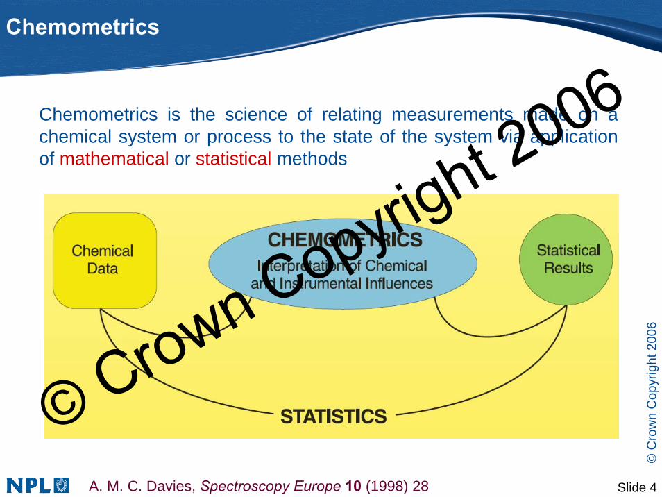
Chemometrics
A. M. C. Davies, Spectroscopy Europe 10 (1998) 28
Chemometrics is the science of relating measurements made on a chemical system or process to the state of the system via application of mathematical or statistical methods
© Crown Copyright 2006

Slide 5
©C
row
n C
opyr
ight
200
6
Chemometrics
• Advantages– Fast and efficient on modern computers– Statistically valid– Removes potential bias– Uses all information available
• Disadvantages– Lots of different methods, procedures, terminologies– Can be difficult to understand
© Crown Copyright 2006

Slide 6
©C
row
n C
opyr
ight
200
6
Data analysis
SIMS DatasetSIMS
Dataset
How is it related to known properties?
What chemicalsare on the surface?
Where are they located?
Calibration / Quantification
Classification
Identification
Can we predictthese properties?
Which group does it belong to?
Is there an outlierin the data?© Crown Copyright 2006

Slide 7
©C
row
n C
opyr
ight
200
6
Data matrix
X has 3 row and 5 columns →3 × 5 data matrix
⎥⎥⎥
⎦
⎤
⎢⎢⎢
⎣
⎡=
6630122412422201821110329
X
Variables
Sam
ples
Mass spectrum of Sample 1
010203040
1 2 3 4 5Mass
Inte
nsity
Mass spectrum of Sample 2
0
10
20
30
1 2 3 4 5Mass
Inte
nsity
Mass spectrum of Sample 3
010203040
1 2 3 4 5Mass
Inte
nsity
© Crown Copyright 2006
Slide 8
©C
row
n C
opyr
ight
200
6
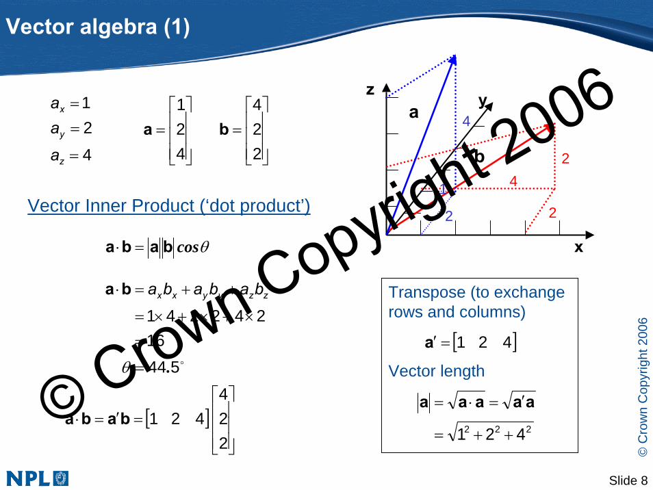
Vector algebra (1)
x
z y
42
2
b⎥⎥⎥
⎦
⎤
⎢⎢⎢
⎣
⎡=
224
ba
2
4
1
⎥⎥⎥
⎦
⎤
⎢⎢⎢
⎣
⎡=
421
a421
=
==
z
y
x
aaa
[ ]⎥⎥⎥
⎦
⎤
⎢⎢⎢
⎣
⎡=′=⋅
224
421baba
Transpose (to exchange rows and columns)
Vector length
[ ]421=′a
222 421 ++=
′=⋅= aaaaa
Vector Inner Product (‘dot product’)
o54416
242241
.=
=×+×+×=
++=⋅
θ
zzyyxx babababa
θcosbaba =⋅
© Crown Copyright 2006

Slide 9
©C
row
n C
opyr
ight
200
6
The smaller is the larger the correlation between a and b
Vector algebra (2)
θcosbaba =′
If then theyare orthogonali.e. at right angles
0=′ba
o90=θ
If they are also of unit lengththen they are orthonormali.e. 1=′aa 1=′bb
Orthogonal vectors are uncorrelated
OrthogonalityIf then the vectors are collinear
o0=θa
b Collinearity ab
If then the vectors are neither orthogonal nor collinear – they are correlated
oo 900 ≠≠θ
Correlation a
b
θ
θ
© Crown Copyright 2006

Slide 10
©C
row
n C
opyr
ight
200
6
Matrix algebra
• A and B must be the same size• Each corresponding element is
added
⎥⎦
⎤⎢⎣
⎡=⎥
⎦
⎤⎢⎣
⎡−
−+⎥
⎦
⎤⎢⎣
⎡493161
210021
683142
CBA =+)()()( KIKIKI ×=×+×
Matrix addition
(e.g. pure spectra + noise = experimental data)
• No. of columns of A must be equal no. of rows of B
• Element in row i and column j of the product matrix AB is equal to row iof A times column j of B
CBA =)())(( KIKNNI ×=××
⎥⎥⎥
⎦
⎤
⎢⎢⎢
⎣
⎡=
⎥⎥⎥
⎦
⎤
⎢⎢⎢
⎣
⎡
×+××+××+××+××+××+×
=⎥⎦
⎤⎢⎣
⎡
⎥⎥⎥
⎦
⎤
⎢⎢⎢
⎣
⎡
121088
1013
222432142222321224213411
2321
242241
Matrix multiplication
© Crown Copyright 2006

Slide 11
©C
row
n C
opyr
ight
200
6
Matrix inversefor a square
matrix
(only exists if matrix is ‘full rank’)
Matrix inverse
IAA =1-
AAI =⎥⎥⎥
⎦
⎤
⎢⎢⎢
⎣
⎡=
100010001
IIdentity matrix: diagonal of 1s
( ) 111 −−− = ABAB
( ) ABAB ′′=′
( ) ++=+ ABAB
Additional properties
Matrix pseudoinverse
for a rectangularmatrix
[ ] 1−′′=+ AAAAIAA =+
CAB +=
CBA =We can now solve matrix equation
If A is square
If A is rectangular
CAB 1−=© Crown Copyright 2006
Slide 12
©C
row
n C
opyr
ight
200
6
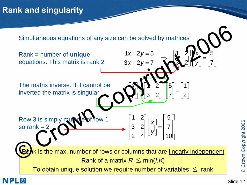
Rank and singularity
723521
=+=+
yxyx
⎥⎦
⎤⎢⎣
⎡=⎥
⎦
⎤⎢⎣
⎡⎥⎦
⎤⎢⎣
⎡⇒
75
2321
yx
Simultaneous equations of any size can be solved by matrices
Rank = number of uniqueequations. This matrix is rank 2
⎥⎥⎥
⎦
⎤
⎢⎢⎢
⎣
⎡=⎥
⎦
⎤⎢⎣
⎡
⎥⎥⎥
⎦
⎤
⎢⎢⎢
⎣
⎡
1075
422321
yxRow 3 is simply multiple of row 1
so rank = 2
⎥⎦
⎤⎢⎣
⎡=⎥
⎦
⎤⎢⎣
⎡⎥⎦
⎤⎢⎣
⎡=⎥
⎦
⎤⎢⎣
⎡−
21
75
2321 1
yxThe matrix inverse. If it cannot be
inverted the matrix is singular
Rank is the max. number of rows or columns that are linearly independentRank of a matrix R min(I,K)
To obtain unique solution we require number of variables rank≤
≤© Crown Copyright 2006

Slide 13
©C
row
n C
opyr
ight
200
6
Matrix projections
yxa 32 +=
a
x
y
[ ] ⎥⎦
⎤⎢⎣
⎡=
yx
32a⎥⎦
⎤⎢⎣
⎡⎥⎦
⎤⎢⎣
⎡ −=⎥
⎦
⎤⎢⎣
⎡**
8705050870
yx
yx
....
To write a in terms of x* and y*, wefind its projections on the new axes
[ ] ⎥⎦
⎤⎢⎣
⎡⎥⎦
⎤⎢⎣
⎡ −=
*
*
....
yx
8705050870
32a
projectionsonto new axes new axes
[ ] ⎥⎦
⎤⎢⎣
⎡=
*
*
..yx6123a
x*
y*
30º
© Crown Copyright 2006

Slide 14
©C
row
n C
opyr
ight
200
6
Data matrixMass spectrum of Sample 1
010203040
1 2 3 4 5Mass
Inte
nsity
Mass spectrum of Sample 2
0
10
20
30
1 2 3 4 5Mass
Inte
nsity
Mass spectrum of Sample 3
010203040
1 2 3 4 5Mass
Inte
nsity
Mass spectrum of Chemical 1
0
2
4
6
8
1 2 3 4 5Mass
Inte
nsity
Mass spectrum of Chemical 2
0
2
4
6
1 2 3 4 5Mass
Inte
nsity
=×
Chemical1
Chemical2
Sample1 5 1
Sample2 2 4
Sample3 0 6
⎥⎥⎥
⎦
⎤
⎢⎢⎢
⎣
⎡
604215
Variables [mass]
Sam
plesSam
ples
Variables [mass]Chemicals
Chem
icalsData matrixChemical spectraSample
composition =×
⎥⎦
⎤⎢⎣
⎡1152440161
⎥⎥⎥
⎦
⎤
⎢⎢⎢
⎣
⎡
6630122412422201821110329
=×
© Crown Copyright 2006

Slide 15
©C
row
n C
opyr
ight
200
6
Data matrix
1. Each spectra can be represented by a vector2. Instead of x, y, z in real space, the axes are mass1, mass2,
mass3… etc in variable space (also ‘data space’)3. Without noise, rank of dataset = number of unique components
4. With random, uncorrelated noise, rank of dataset = number of samples or number of variables, whichever is smaller
⎥⎥⎥
⎦
⎤
⎢⎢⎢
⎣
⎡
604215
Variables [mass]
Sam
plesSam
ples
Variables [mass]Chemicals
Chem
icalsData matrixChemical spectraSample
composition =×
⎥⎦
⎤⎢⎣
⎡1152440161
⎥⎥⎥
⎦
⎤
⎢⎢⎢
⎣
⎡
6630122412422201821110329
=×
© Crown Copyright 2006
Slide 16
©C
row
n C
opyr
ight
200
6
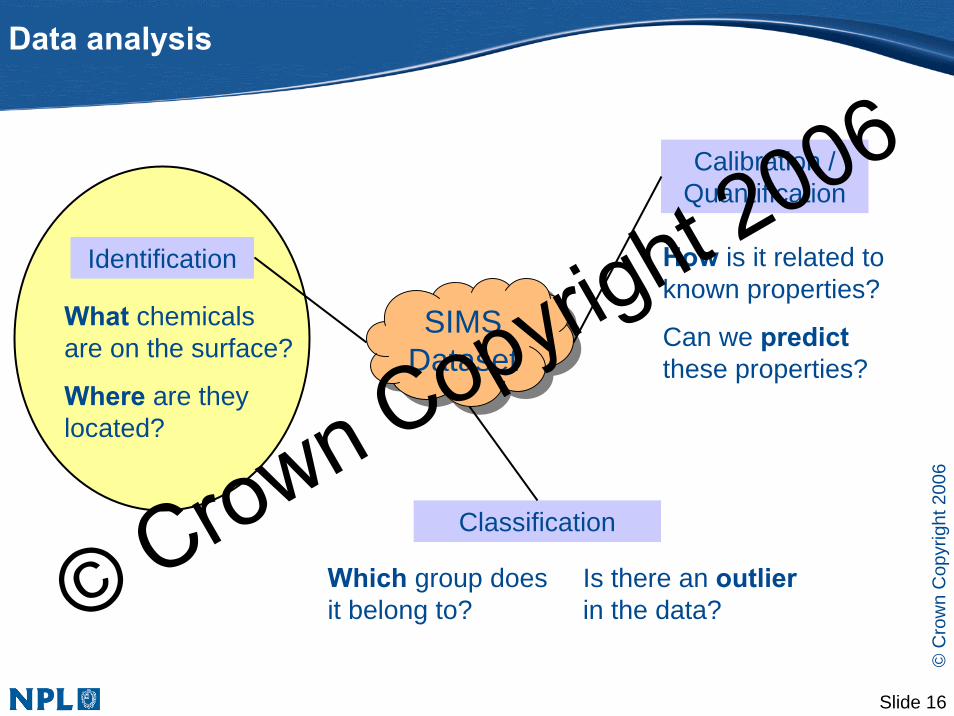
Data analysis
SIMS DatasetSIMS
Dataset
How is it related to known properties?
Where are they located?
What chemicalsare on the surface?
Calibration / Quantification
Classification
Identification
Can we predictthese properties?
Which group does it belong to?
Is there an outlierin the data?© Crown Copyright 2006

Slide 17
©C
row
n C
opyr
ight
200
6
Terminology
Terms used here PCA MCR PLS
factors P loadings,
eigenvector, principal component
component spectra
latent vectors, latent variables
projections T scores component concentration scores
In order to clarify existing terminology and emphasise the relationship between the different chemometrics techniques, the following terminology is adopted in this tutorial –
© Crown Copyright 2006
Slide 18
©C
row
n C
opyr
ight
200
6
Principal component analysis (PCA)
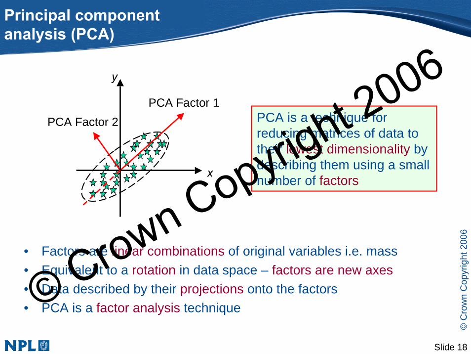
x
y
PCA Factor 1PCA Factor 2
• Factors are linear combinations of original variables i.e. mass• Equivalent to a rotation in data space – factors are new axes• Data described by their projections onto the factors• PCA is a factor analysis technique
PCA is a technique for reducing matrices of data to their lowest dimensionality by describing them using a small number of factors
© Crown Copyright 2006
Slide 19
©C
row
n C
opyr
ight
200
6
Principal component analysis (PCA)
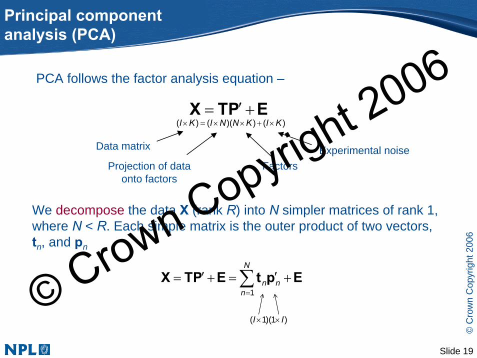
PCA follows the factor analysis equation –
Data matrix
Projection of dataonto factors
FactorsExperimental noise
EPTX +′=)())(()( KIKNNIKI ×+××=×
EptEPTX +′=+′= ∑=
N
nnn
1
)1)(1( II ×
We decompose the data X (rank R) into N simpler matrices of rank 1, where N < R. Each simple matrix is the outer product of two vectors, tn, and pn
ש Crown Copyright 2006
Slide 20
©C
row
n C
opyr
ight
200
6
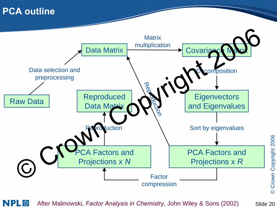
Raw Data
Data Matrix
Data selection and preprocessing
PCA outline
Covariance Matrix
Matrix multiplication
Eigenvectors and Eigenvalues
Decomposition
PCA Factors and Projections x R
Sort by eigenvaluesReproduction
ReproducedData Matrix
Reproduction
PCA Factors and Projections x N
Factor compression
After Malinowski, Factor Analysis in Chemistry, John Wiley & Sons (2002)
© Crown Copyright 2006

Slide 21
©C
row
n C
opyr
ight
200
6
Raw Data
Data Matrix
Data selection and preprocessing
PCA outline
Covariance Matrix
Matrix multiplication
Eigenvectors and Eigenvalues
Decomposition
PCA Factors and Projections x R
Sort by eigenvaluesReproduction
ReproducedData Matrix
Reproduction
PCA Factors and Projections x N
Factor compression
After Malinowski, Factor Analysis in Chemistry, John Wiley & Sons (2002)
© Crown Copyright 2006
Slide 22
©C
row
n C
opyr
ight
200
6
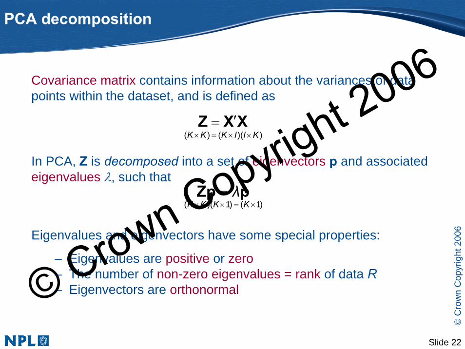
Covariance matrix contains information about the variances of data points within the dataset, and is defined as
PCA decomposition
XXZ ′=))(()( KIIKKK ××=×
pZp λ=
In PCA, Z is decomposed into a set of eigenvectors p and associated eigenvalues λ, such that
)1()1)((
Eigenvalues and eigenvectors have some special properties:
– Eigenvalues are positive or zero– The number of non-zero eigenvalues = rank of data R– Eigenvectors are orthonormal
×=×× KKKK
© Crown Copyright 2006

Slide 23
©C
row
n C
opyr
ight
200
6
Raw Data
Data Matrix
Data selection and preprocessing
PCA outline
Covariance Matrix
Eigenvectors and Eigenvalues
Decomposition
PCA Factors and Projections x R
Sort by eigenvaluesReproduction
ReproducedData Matrix
Reproduction
PCA Factors and Projections x N
Factor compression
After Malinowski, Factor Analysis in Chemistry, John Wiley & Sons (2002)
Matrix multiplication
© Crown Copyright 2006

Slide 24
©C
row
n C
opyr
ight
200
6
PCA factors
• Because Z is the covariance matrix, eigenvectors of Z are special directions in the data space that is optimal in describing the variance of the data
• Eigenvalues are the amount of variance described by their associated eigenvector
∑=
′=′=R
nnn
1ptPTX
Projection of data onto nth factor
(scores)The nth factor
(loadings)
• These eigenvectors are the factors PCA obtain for the factor analysis equation. They are sorted by their eigenvalues
• PCA factors successively capture the largest amount of variance (spread) within the dataset
• Projection of data onto factors (often called scores) are orthogonal© Crown Copyright 2006

Slide 25
©C
row
n C
opyr
ight
200
6
x
y
PCA Factor 1PCA Factor 2
• The first factor lies along the major axis of ellipse and accounts for most variation
• Instead of describing the data using correlated variables x and y, we transform them onto a new basis (factors) which are uncorrelated
• By removing higher factors (variances due to noise) we can reduce dimensionality of data ⇒‘factor compression’
PCA – graphical representation
© Crown Copyright 2006

Slide 26
©C
row
n C
opyr
ight
200
6
Raw Data
Data Matrix
Data selection and preprocessing
PCA outline
Covariance Matrix
Matrix multiplication
Eigenvectors and Eigenvalues
Decomposition
PCA Factors and Projections x R
Sort by eigenvaluesReproduction
ReproducedData Matrix
Reproduction
PCA Factors and Projections x N
Factor compression
After Malinowski, Factor Analysis in Chemistry, John Wiley & Sons (2002)
© Crown Copyright 2006

Slide 27
©C
row
n C
opyr
ight
200
6
Number of factors
1 2 3 4 5 6 7 810-15
10-10
10-5
100
105
1010
Eig
enva
lue
1 2 3 4 5 6 7 8101
102
103
104
105
106
107
108
Sorted eigenvector index
(a)
(b)
Data set of 8 spectra from mixing 3 pure compound spectra
no noise
Poisson noisemax 5000 counts
1. Prior knowledge of system
2. ‘Scree test’:Eigenvalue plot levels off in a linearly decreasing manner after 3 factors
3. Percentage of variance captured by Nth
eigenvector:
4. Percentage of total variance captured by N eigenvectors:
%100seigenvalue all of sum
eigenvalue th
×N
%100seigenvalue all of sum
to up seigenvalue of sum×
N
Eig
enva
lue
© Crown Copyright 2006

Slide 28
©C
row
n C
opyr
ight
200
6
Data reproduction
X is the reproduced data matrix• reproduced from N selected factors
and projections• noise filtered by removal of higher
factors that describe noise variations
• useful for MCR
EptEPTX +′=+′= ∑=
N
nnn
1
PTEXX ′=−=
E is the matrix of residuals• should contain noise only• useful for judging quality of PCA model• may show up unexpected features!
XXE −=
∑=
′−=N
nnn
1ptXE© Crown Copyright 2006

Slide 29
©C
row
n C
opyr
ight
200
6
Raw Data
Data Matrix
Data selection and preprocessing
PCA outline
Covariance Matrix
Matrix multiplication
Eigenvectors and Eigenvalues
Decomposition
PCA Factors and Projections x R
Sort by eigenvaluesReproduction
ReproducedData Matrix
Reproduction
PCA Factors and Projections x N
Factor compression
After Malinowski, Factor Analysis in Chemistry, John Wiley & Sons (2002)
© Crown Copyright 2006

Slide 30
©C
row
n C
opyr
ight
200
6
• Enhances PCA by bringing out important variance in dataset• Makes assumption about nature of variance in data• Can distort interpretation and quantification
• Includes:– mass binning– peak selection– mean centering– normalisation – variance scaling– Poisson scaling– logarithmic transformation
Data preprocessing
More details in the following slides
© Crown Copyright 2006

Slide 31
©C
row
n C
opyr
ight
200
6
• Subtract mean spectrum from each sample• PCA describes variations from the mean
Mean centering
x
z
Factor 2
Factor 1y
Raw data
1st factor goes from origin to centre of gravity of data
y
z
Factor 1
x
Factor 2
Mean Centering
1st factor goes from origin and accounts for the highest variance
( ),ki,ki,k :XXX mean−=~Preprocessed datasample i, mass k Raw data
sample i, mass kMean intensity of mass k
© Crown Copyright 2006
Slide 32
©C
row
n C
opyr
ight
200
6
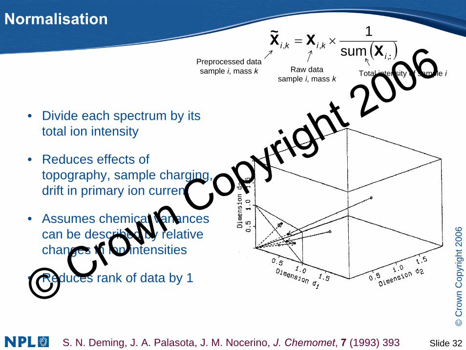
Normalisation
• Divide each spectrum by its total ion intensity
• Reduces effects of topography, sample charging, drift in primary ion current
• Assumes chemical variances can be described by relative changes in ion intensities
• Reduces rank of data by 1
S. N. Deming, J. A. Palasota, J. M. Nocerino, J. Chemomet, 7 (1993) 393
( ):XXX
,,, sum
1i
kiki ×=~
Preprocessed datasample i, mass k Total intensity of sample iRaw data
sample i, mass k
© Crown Copyright 2006

Slide 33
©C
row
n C
opyr
ight
200
6
Variance scaling
• Divide each variable by its variance in the dataset• Equalises importance of each variable (i.e. mass)• Problematic for weak peaks – usually used with peak selection• Called ‘auto scaling’ if combined with mean centering
Var
ianc
e
Mean
For each variable (mass, in SIMS spectrum)
Raw data Mean-centering
Variance scaling
Auto scaling
P. Geladi and B. Kowalski, Partial Least-Squares Regression: A Tutorial,Analytica Chimica Acta, 185 (1986) 1
( )kkiki
,,, var
1:X
XX ×=~
Preprocessed datasample i, mass k Variance of mass kRaw data
sample i, mass k
© Crown Copyright 2006
Slide 34
©C
row
n C
opyr
ight
200
6
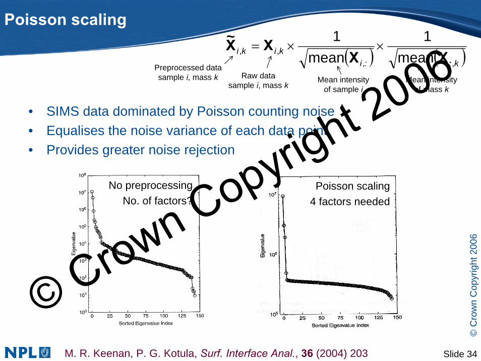
Poisson scaling
( )
• SIMS data dominated by Poisson counting noise• Equalises the noise variance of each data point• Provides greater noise rejection
M. R. Keenan, P. G. Kotula, Surf. Interface Anal., 36 (2004) 203
( )k:ikiki
,,,, mean
1mean
1
:
~XX
XX ××=
No preprocessingNo. of factors?
Poisson scaling4 factors needed
Preprocessed datasample i, mass k Mean intensity
of mass k
Raw datasample i, mass k
Mean intensityof sample i
© Crown Copyright 2006

Slide 35
©C
row
n C
opyr
ight
200
6
Data preprocessingsummary
Method of preprocessing Effect of preprocessing
No preprocessing First factor goes from origin to mean of data
Mean centering All factors describe variations from the mean
Normalisation Equalises total ion yield of each sample and emphasise relative changes in ion intensities
Variance scaling Equalises variance of every peak regardless of intensity. Best with peak selection.
Poisson scaling Equalises noise variance of each data point. Provides greater noise rejection.© Crown Copyright 2006

Slide 36
©C
row
n C
opyr
ight
200
6
PCA example (1)
• Three protein compositions (100% fibrinogen, 50% fibrinogen / 50% albumin, 100% albumin) adsorbed onto poly(DTB suberate)
• First factor (PC1) shows relative abundance of amino acid peaks of two proteins
• Projection onto first factor separates samples based on protein composition
D.J. Graham et al, Appl. Surf. Sci., 252 (2006) 6860
PCA
Fac
tor 1
(62%
)P
CA
Pro
ject
ions
1 (6
2%)
Fib
Alb
© Crown Copyright 2006

Slide 37
©C
row
n C
opyr
ight
200
6
PCA example (2)
• 16 different single protein films adsorbed on mica
• Excellent classification of proteins using only 2 factors
• Factors consistent with total amino acid composition of various proteins
• 95% confidence limits provide means for identification / classification
M. Wagner & D. G. Castner, Langmuir, 17 (2001) 4649
PC
A P
roje
ctio
ns 2
(19%
)
PCA Projections 1 (53%)
PC
A F
acto
rs
© Crown Copyright 2006
Slide 38
©C
row
n C
opyr
ight
200
6
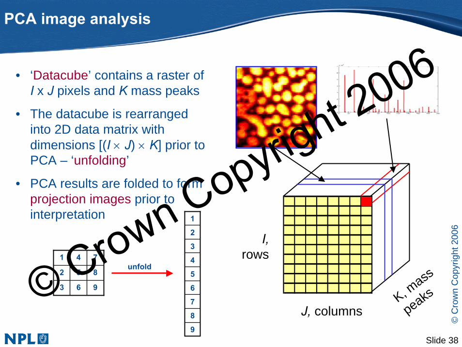
PCA image analysis
I, rows
K, mass
peaksJ, columns
• ‘Datacube’ contains a raster of I x J pixels and K mass peaks
• The datacube is rearranged into 2D data matrix with dimensions [(I × J) × K] prior to PCA – ‘unfolding’
• PCA results are folded to form projection images prior to interpretation
9
8
7
6
5
4
3
2
1
963
852
741unfold
© Crown Copyright 2006

Slide 39
©C
row
n C
opyr
ight
200
6
2 4 6 8 10 12 14 16 18 20
0
0.2
0.4
0.6
0.8
Sorted eigenvector index
log(
eige
nval
ues)
2 4 6 8 10 12 14 16 18 20-2
-1
0
1
2
Sorted eigenvector index
log(
eige
nval
ues)
2 4 6 8 10 12 14 16 18 20-5
-4.5-4
-3.5-3
-2.5-2
-1.5
Sorted eigenvector index
log(
eige
nval
ues)
PCA image example (1)
Immiscible PC / PVC polymer blend42 counts per pixel on average
Total ion image
Mean centering
Normalisation
Poisson scaling
Only 2 factors needed –dimensionality of image reduced by factor of 20!
J. Lee, I. S. Gilmore, to be published
© Crown Copyright 2006

Slide 40
©C
row
n C
opyr
ight
200
6
PCA image example (1)
-2
0
2
4
6
8
10
-5
0
5
10
0 5 10 15 20 25 30 35 40-0.5
0
0.5
1
1.5
2
Mass, u
Poisson scaled PCA results after mean centering
0 5 10 15 20 25 30 35 40-0.4
-0.2
0
0.2
0.4
0.6
0.8
1
Mass, u
1st factor distinguishes PVC and PC phases
2nd factor shows detector saturation for intense 35Cl peak
J. Lee, I. S. Gilmore, to be published
© Crown Copyright 2006
Slide 41
©C
row
n C
opyr
ight
200
6
PCA image example (2)
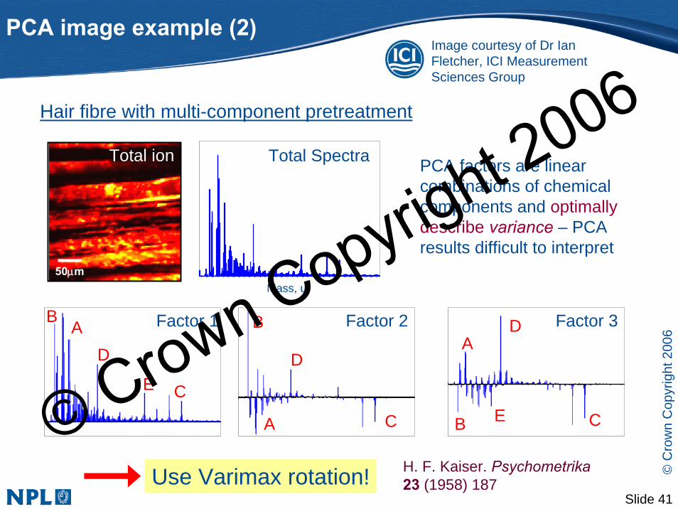
Hair fibre with multi-component pretreatment
Mass, u
Total Spectra
50μm
Total ion PCA factors are linear combinations of chemical components and optimally describe variance – PCA results difficult to interpret
AD
CE
B B
C
D
A
D
C
A
EB
Use Varimax rotation!
Factor 1 Factor 2 Factor 3
H. F. Kaiser. Psychometrika23 (1958) 187
Image courtesy of Dr Ian Fletcher, ICI Measurement Sciences Group
© Crown Copyright 2006

Slide 42
©C
row
n C
opyr
ight
200
6
PCA image example (2)
Factor 1A
Factor 2
Factor 3
B
C
Factor 4
Factor 5
D
E
Mass, u
After Varimax rotation, distribution and characteristic
peaks are obtained, simplifying interpretation of huge dataset
Mass, u© Crown Copyright 2006

Slide 43
©C
row
n C
opyr
ight
200
6
Multivariate curve resolution (MCR)
• PCA factors are directions that describes variance– positive and negative peaks in factors– can be difficult to interpret
• We want to resolve original chemical spectra and reverse the following process:
• Use multivariate curve resolution (also called ‘self modelling mixture analysis’)
⎥⎥⎥
⎦
⎤
⎢⎢⎢
⎣
⎡=⎥
⎦
⎤⎢⎣
⎡
⎥⎥⎥
⎦
⎤
⎢⎢⎢
⎣
⎡
6630122412422201821110329
1152440161
604215
Variables
Sam
plesS
ampl
es
VariablesChemicals
Chem
icals
Data matrixChemical spectraSample composition =×
© Crown Copyright 2006

Slide 44
©C
row
n C
opyr
ight
200
6
Multivariate curve resolution (MCR)
MCR is designed for recovery of chemical spectra and contributions from a multi-component mixture, when little or no prior information about the composition is available
MCR uses an iterative least-squares algorithm to extract solutions, while applying suitable constraints e.g. non-negativity
Data matrix
Projection of dataonto factors
FactorsExperimental noise
EPTX +′=)())(()( KIKNNIKI ×+××=×
x
y MCR Factor 2
MCR Factor 1
© Crown Copyright 2006

Slide 45
©C
row
n C
opyr
ight
200
6
Multivariate curve resolution (MCR)
1. Determine number of factors N via eigenvalue plot2. Obtain PCA reproduced data matrix for N factors3. Obtain initial estimates of spectra (factors) or contributions (projections)
• Random initialisation• PCA factors• Varimax rotated PCA factors• Pure variable detection algorithm e.g. SIMPLISMA
4. Constraints• Non-negativity• Equality
5. Convergence criterion6. Alternating least squares (ALS) optimisation
Six Steps to MCR Results
© Crown Copyright 2006
Slide 46
©C
row
n C
opyr
ight
200
6
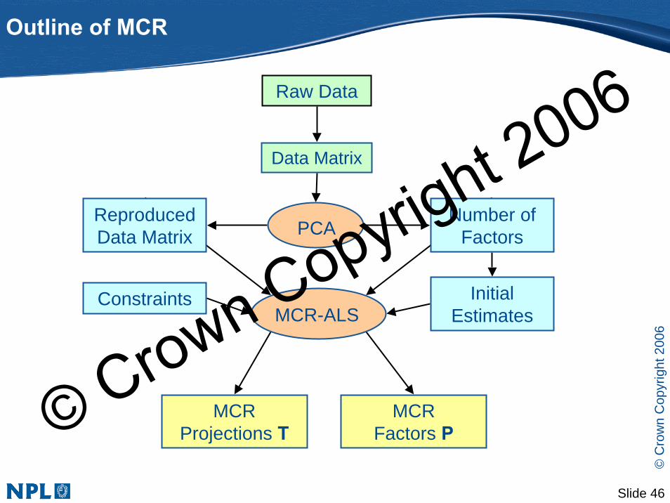
Outline of MCR
Raw Data
Data Matrix
Constraints
MCR Projections T
MCRFactors P
MCR-ALS
ReproducedData Matrix
Initial Estimates
Number of FactorsPCA
© Crown Copyright 2006

Slide 47
©C
row
n C
opyr
ight
200
6
• Start with PCA reproduced data matrix
• Assume initial estimate of factors P
• Steps (1) – (4) are repeated until MCR factors P and projections Tare able to reconstruct reproduced data matrix X within acceptable error specified in convergence criterion
MCR-ALS algorithm
PTX ′=
( )
M
XXE
PTX
XTP
PXT
−=
′=
+=′
+′=
ˆ
ˆ
(1) Find estimate of T using P, applying constraints
(2) Find new estimate of P using T, applying constraints(3) Compute MCR reproduced matrix
(4) Compare results and check convergence
[ ] 1−′′=+ AAAA
Pseudoinverse of rectangular matrix
© Crown Copyright 2006

Slide 48
©C
row
n C
opyr
ight
200
6
• MCR can suffer from rotational ambiguity• Accuracy of resolved spectra depends on ‘selectivity’ i.e. existence
of pixels or sample where there is only contribution from one component
• Good initial estimates are essential• Peaks for the intense components may appear in spectra resolved
for weak component
Rotational ambiguity
x
y MCR Factor 2
MCR Factor 1Chemical 2?
x
y Chemical 1?
© Crown Copyright 2006

Slide 49
©C
row
n C
opyr
ight
200
6
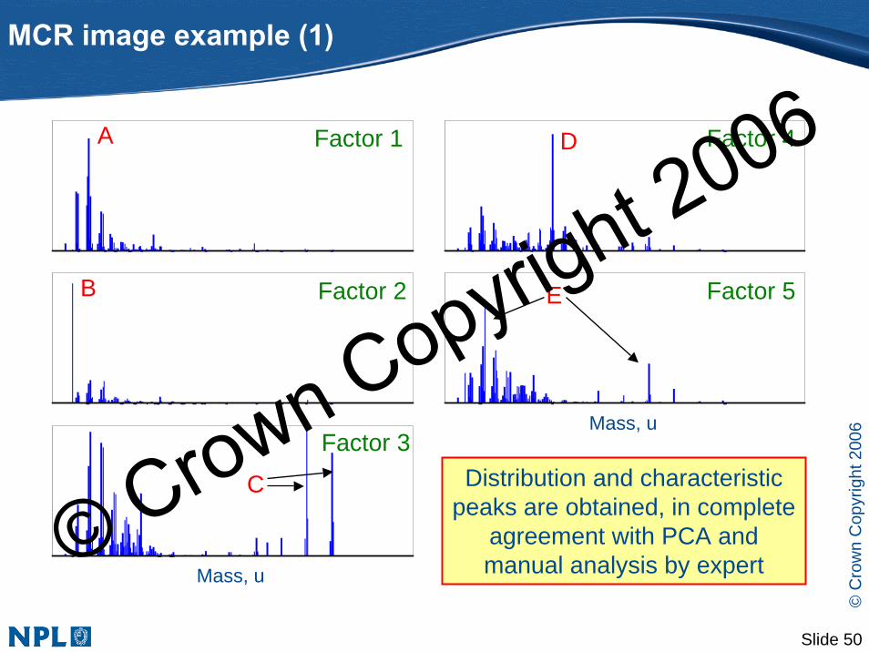
MCR image example (1)
Hair fibre with multi-component pretreatment
Mass, u
Total Spectra
Projections 1 Projections 3 Projections 4 Projections 5Projections 2
Image courtesy of Dr Ian Fletcher, ICI Measurement Sciences Group
50μm
Total ion
© Crown Copyright 2006
Slide 50
©C
row
n C
opyr
ight
200
6
Factor 1A
Factor 2
Factor 3
Factor 4
Factor 5B
C
D
E
Mass, u
Distribution and characteristic peaks are obtained, in complete
agreement with PCA and manual analysis by expert
MCR image example (1)
Mass, u© Crown Copyright 2006
Slide 51
©C
row
n C
opyr
ight
200
6
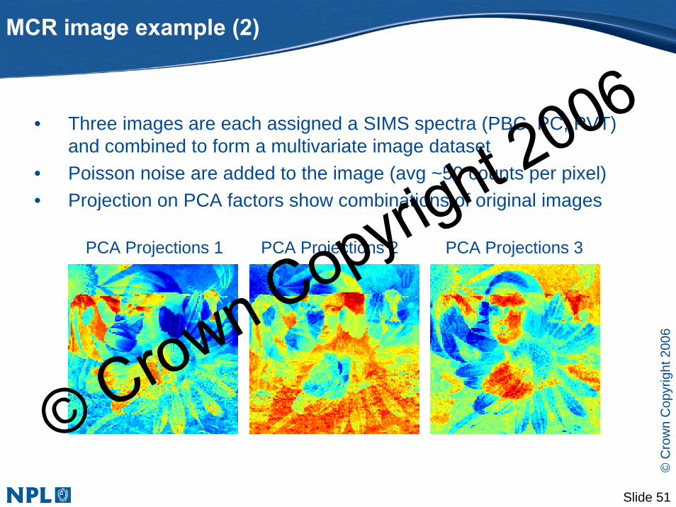
MCR image example (2)
• Three images are each assigned a SIMS spectra (PBC, PC, PVT) and combined to form a multivariate image dataset
• Poisson noise are added to the image (avg ~50 counts per pixel)• Projection on PCA factors show combinations of original images
PCA Projections 1 PCA Projections 2 PCA Projections 3
© Crown Copyright 2006

Slide 52
©C
row
n C
opyr
ight
200
6
MCR image example (2)
MCR resolves the original images and spectra unambiguously!
MCR Projections 1 MCR Projections 2 MCR Projections 3
© Crown Copyright 2006

Slide 53
©C
row
n C
opyr
ight
200
6
Data analysis
SIMS DatasetSIMS
Dataset
How is it related to known properties?What chemicals
are on the surface?
Where are they located?
Calibration / Quantification
Classification
Identification
Can we predictthese properties?
Which group does it belong to?
Is there an outlierin the data?© Crown Copyright 2006

Slide 54
©C
row
n C
opyr
ight
200
6
Regression analysis
Mass spectrum of Sample 1
010203040
1 2 3 4 5Mass
Inte
nsity
Mass spectrum of Sample 2
0
10
20
30
1 2 3 4 5Mass
Inte
nsity
Mass spectrum of Sample 3
010203040
1 2 3 4 5Mass
Inte
nsity
XPS measurement
Molecular weight
Density
Sample 1 5 1
4
6
3
Sample 2 2 7
Sample 3 1 4
Measured properties
We can build a model to predict the properties of materials from their SIMS spectra
( )exbxbxbxby
efy
mm +++++=+=
...332211
x
Dependent variablei.e. measured property
Independent variablei.e. intensity at mass m
Regressioncoefficient
© Crown Copyright 2006
Slide 55
©C
row
n C
opyr
ight
200
6
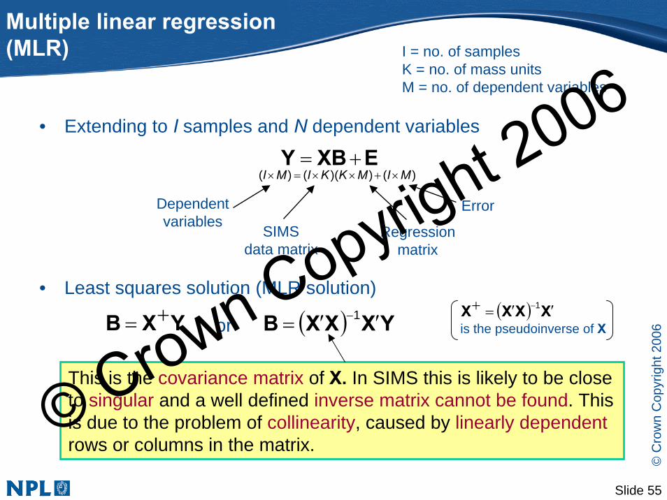
Multiple linear regression (MLR)
E• Extending to I samples and N dependent variables
XBY +=
Dependentvariables
SIMSdata matrix
Regressionmatrix
Error
)())(()( MIMKKIMI ×+××=×
I = no. of samplesK = no. of mass unitsM = no. of dependent variables
• Least squares solution (MLR solution)
( ) YXXXB ′′= −1
This is the covariance matrix of X. In SIMS this is likely to be close to singular and a well defined inverse matrix cannot be found. This is due to the problem of collinearity, caused by linearly dependentrows or columns in the matrix.
YXB += or( ) XXXX ′′=+ −1
is the pseudoinverse of X
© Crown Copyright 2006

Slide 56
©C
row
n C
opyr
ight
200
6
MLR - graphical representation EXBY +=
Dependentvariables
SIMSdata matrix
Regressionmatrix
Error
We relate Y to the projection of X onto B –
MLR finds the least squares solution i.e. the best R2 correlationbetween Y and the projections of data onto the regression vector XB
A. M. C. Davies, T. Fearn, Spectroscopy Europe 17 (2005) 28
Large number of variables (e.g. mass) → Risk of overfitting!© Crown Copyright 2006
Slide 57
©C
row
n C
opyr
ight
200
6
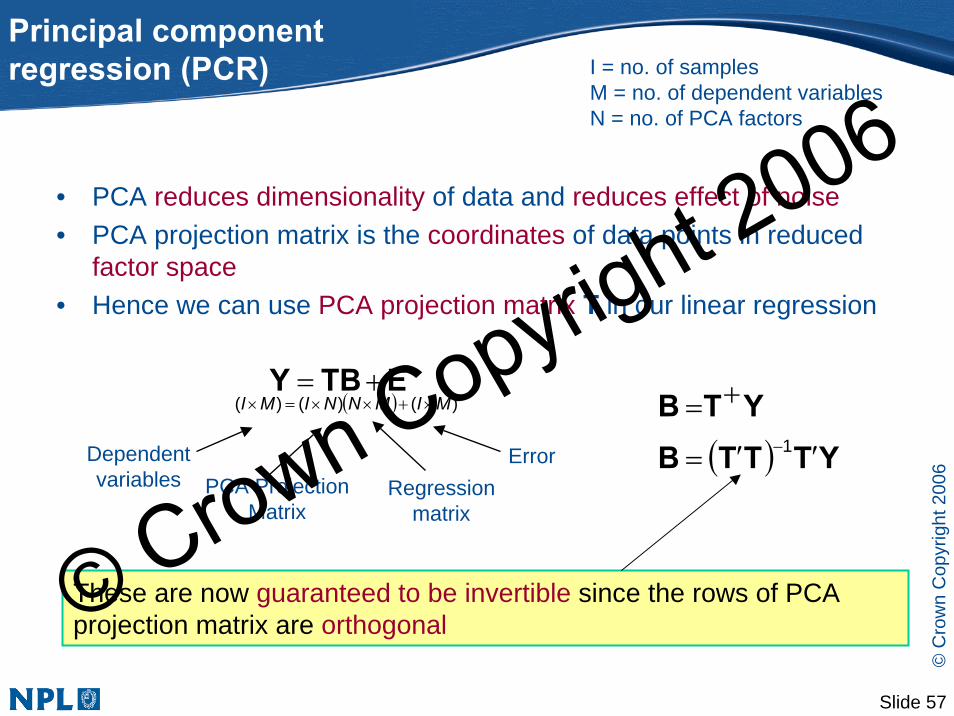
Principal component regression (PCR)
• PCA reduces dimensionality of data and reduces effect of noise• PCA projection matrix is the coordinates of data points in reduced
factor space• Hence we can use PCA projection matrix T in our linear regression
( ) YTTTBYTB
′′=
+=−1
ETB
I = no. of samplesM = no. of dependent variablesN = no. of PCA factors
Y +=
Dependentvariables PCA Projection
MatrixRegression
matrix
Error
( ) )()()( MIMNNIMI ×+××=×
These are now guaranteed to be invertible since the rows of PCA projection matrix are orthogonal© Crown Copyright 2006
Slide 58
©C
row
n C
opyr
ight
200
6
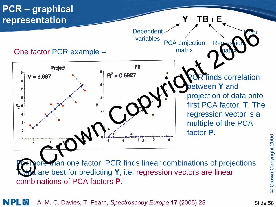
PCR – graphical representation
A. M. C. Davies, T. Fearn, Spectroscopy Europe 17 (2005) 28
One factor PCR example –
PCR finds correlation between Y and projection of data onto first PCA factor, T. The regression vector is a multiple of the PCA factor P.
For more than one factor, PCR finds linear combinations of projections T that are best for predicting Y, i.e. regression vectors are linear combinations of PCA factors P.
EΤΒY +=Dependentvariables
PCA projectionmatrix
Regressionmatrix
Error
© Crown Copyright 2006
Slide 59
©C
row
n C
opyr
ight
200
6
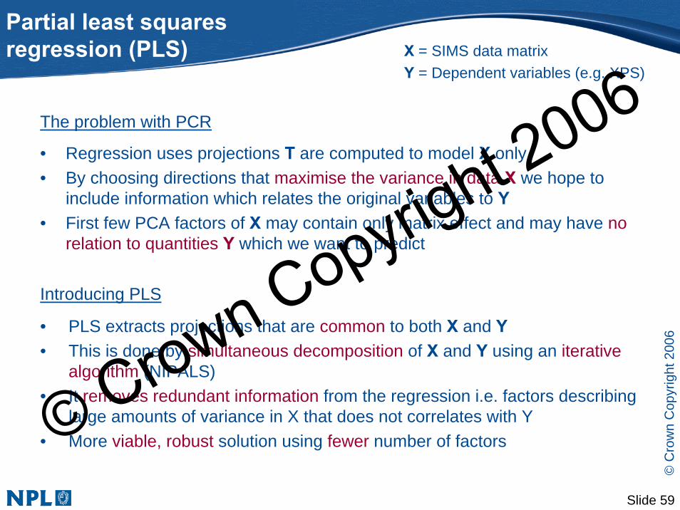
Partial least squares regression (PLS)
The problem with PCR
• Regression uses projections T are computed to model X only• By choosing directions that maximise the variance in data X we hope to
include information which relates the original variables to Y• First few PCA factors of X may contain only matrix effect and may have no
relation to quantities Y which we want to predict
X = SIMS data matrixY = Dependent variables (e.g. XPS)
Introducing PLS
• PLS extracts projections that are common to both X and Y• This is done by simultaneous decomposition of X and Y using an iterative
algorithm (NIPALS)• It removes redundant information from the regression i.e. factors describing
large amounts of variance in X that does not correlates with Y• More viable, robust solution using fewer number of factors© Crown Copyright 2006
Slide 60
©C
row
n C
opyr
ight
200
6
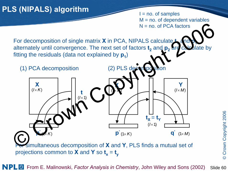
PLS (NIPALS) algorithm
For decomposition of single matrix X in PCA, NIPALS calculate t1 and p1alternately until convergence. The next set of factors t2 and p2 are calculate by fitting the residuals (data not explained by p1)
From E. Malinowski, Factor Analysis in Chemistry, John Wiley and Sons (2002)
(1) PCA decomposition
Xt
p’
)( KI ×
)1( ×I
)1( K×
For simultaneous decomposition of X and Y, PLS finds a mutual set of projections common to X and Y so tx = ty
(2) PLS decomposition
tX = tY
Y
q’p’ )1( K×
X)( KI ×
)1( M×
)( MI ×
)1( ×I
I = no. of samplesM = no. of dependent variablesN = no. of PCA factors
© Crown Copyright 2006

Slide 61
©C
row
n C
opyr
ight
200
6
We can now write
PLS formulation
• T are PLS projections used to predict Y from X (often referred to as ‘scores’)• W is the weights matrix and reflects covariance structure between X and Y• P and Q are not orthogonal matrices due to constraint on finding common
projections T. They are sometimes called ‘x-loadings’ and ‘y-loadings’ respectively
• In literature ‘latent variable’ refers to the set of quantities t, p and qassociated with each PLS factor
EXBY +=FQTYEPTX+′=+′=
( ) QWQPYXB ′=′+′=+=
projections errors regression vector weights matrix
© Crown Copyright 2006

Slide 62
©C
row
n C
opyr
ight
200
6
200 400 600 800 1000 1200-2
0
2
4
6
8
10
12x 1010
Mass, u
Reg
ress
ion
Vec
tor f
or Y
0 1 2 3 4 5 60
1
2
3
4
5
6
Thickness measured by XPS (nm)
Thic
knes
s pr
edic
ted
by S
IMS
(nm
)
PLS example (1)
• SIMS spectra of thin films of Irganox were compared with their thicknesses measured with XPS
• PLS model able to predict thicknesses for t < 6nm• PLS regression vector shows us the SIMS peaks most correlated
with thicknesses
231
1176
59
277
J. Lee, I. S. Gilmore, to be published
© Crown Copyright 2006

Slide 63
©C
row
n C
opyr
ight
200
6
PLS example (2)
A. Chilkoti, A.E Scheimer, V.H Perez Luna and B.D Ratner, Anal. Chem. 67 (1995) 2883
• Surfaces of plasma deposited films were characterised by SIMS. This was then related to bovine arterial endothelial cell (BAEC) growth (cell counting)
• Allowed surface treatment to be characterised
• Reduces amount of biological cell counting experiments required
Cells counted optically
PLS
pre
dict
ion
from
TOF-
SIM
S d
ata
© Crown Copyright 2006
Slide 64
©C
row
n C
opyr
ight
200
6
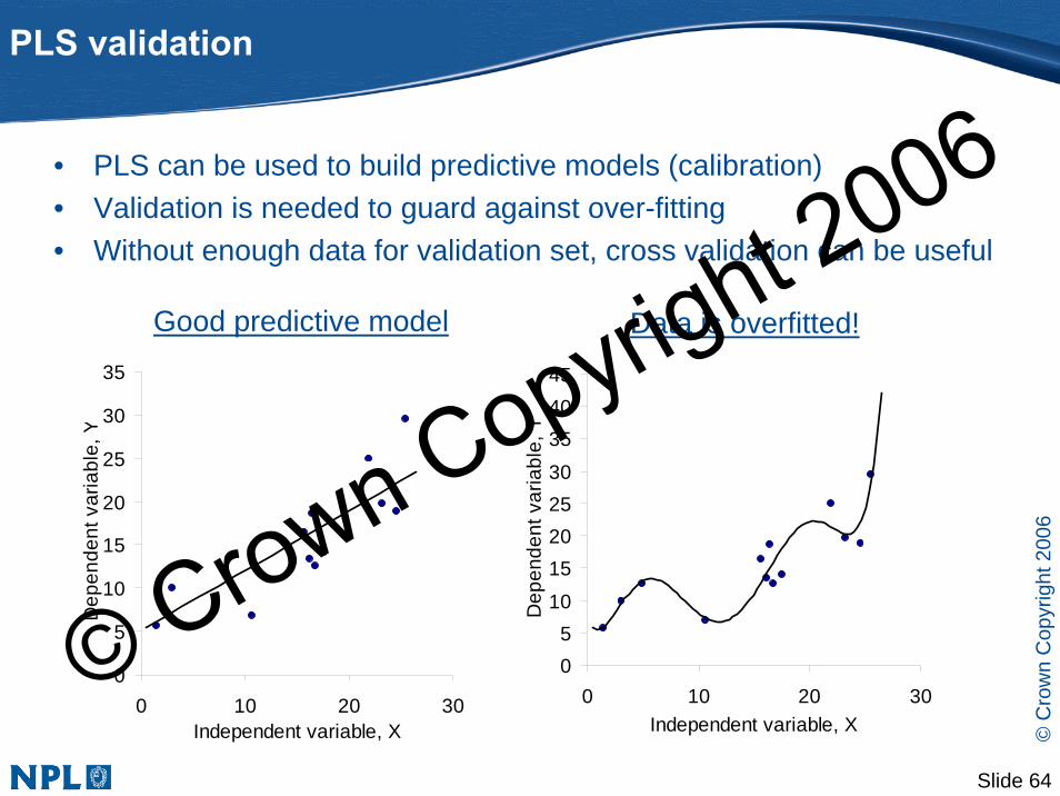
PLS validation
• PLS can be used to build predictive models (calibration)• Validation is needed to guard against over-fitting• Without enough data for validation set, cross validation can be useful
0
5
10
15
20
25
30
35
0 10 20 30Independent variable, X
Dep
ende
nt v
aria
ble,
Y
05
10
15202530
354045
0 10 20 30Independent variable, X
Dep
ende
nt v
aria
ble,
Y
Good predictive model Data is overfitted!
© Crown Copyright 2006

Slide 65
©C
row
n C
opyr
ight
200
6
1 2 3 4 5 6 7 8 9 10 11 120
0.1
0.2
0.3
0.4
0.5
0.6
0.7
Number of PLS Factors
RM
SE
CV
, RM
SE
C
RMSECVRMSEC
PLS validation
• ‘Leave one out’ cross validation most popular– Calculate PLS model excluding sample i– Predict sample i– Repeat for all different samples– Calculate root mean square error of prediction
RMSEC (Root Mean Square Error of Calibration) goes down with increasing number of factors
To decide optimal number of factors use minimum of RMSECV(Root Mean Square Error of Cross Validation) or PRESS (Prediction Residual Sum of Squares)© Crown Copyright 2006
Slide 66
©C
row
n C
opyr
ight
200
6
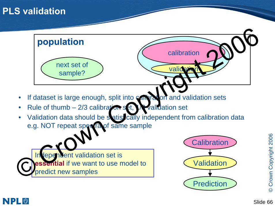
PLS validation
• If dataset is large enough, split into calibration and validation sets• Rule of thumb – 2/3 calibration set, 1/3 validation set• Validation data should be statistically independent from calibration data
e.g. NOT repeat spectra of same sample
sample
populationcalibration
validationnext set ofsample?
Calibration
Validation
Prediction
Independent validation set is essential if we want to use model to predict new samples© Crown Copyright 2006

Slide 67
©C
row
n C
opyr
ight
200
6
Data analysis
SIMS DatasetSIMS
Dataset
How is it related to known properties?What chemicals
are on the surface?
Where are they located?
Calibration / Quantification
Classification
Identification
Can we predictthese properties?
Which group does it belong to?
Is there an outlierin the data?© Crown Copyright 2006
Slide 68
©C
row
n C
opyr
ight
200
6
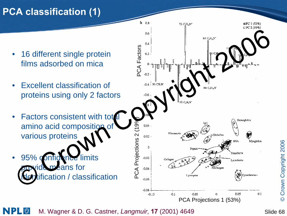
PCA classification (1)
• 16 different single protein films adsorbed on mica
• Excellent classification of proteins using only 2 factors
• Factors consistent with total amino acid composition of various proteins
• 95% confidence limits provide means for identification / classification
M. Wagner & D. G. Castner, Langmuir, 17 (2001) 4649
PC
A P
roje
ctio
ns 2
(19%
)
PCA Projections 1 (53%)
PC
A F
acto
rs
© Crown Copyright 2006
Slide 69
©C
row
n C
opyr
ight
200
6
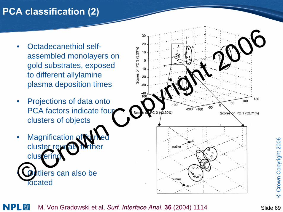
PCA classification (2)
• Octadecanethiol self-assembled monolayers on gold substrates, exposed to different allylamine plasma deposition times
• Projections of data onto PCA factors indicate four clusters of objects
• Magnification of framed cluster reveals further clustering
• Outliers can also be located
M. Von Gradowski et al, Surf. Interface Anal. 36 (2004) 1114
© Crown Copyright 2006

Slide 70
©C
row
n C
opyr
ight
200
6
• PC-DFA = “Principal Component – Discriminant Function Analysis”• ‘Discriminant functions’ maximizes the Fisher’s ratio between groups
• Used to distinguish strains of bacteria
PC-DFA
( )21
221ratio sFisher'
varvarmeanmean+−
=
J. S. Fletcher et al, Appl. Surf. Sci. 252 (2006) 6869
© Crown Copyright 2006
Slide 71
©C
row
n C
opyr
ight
200
6
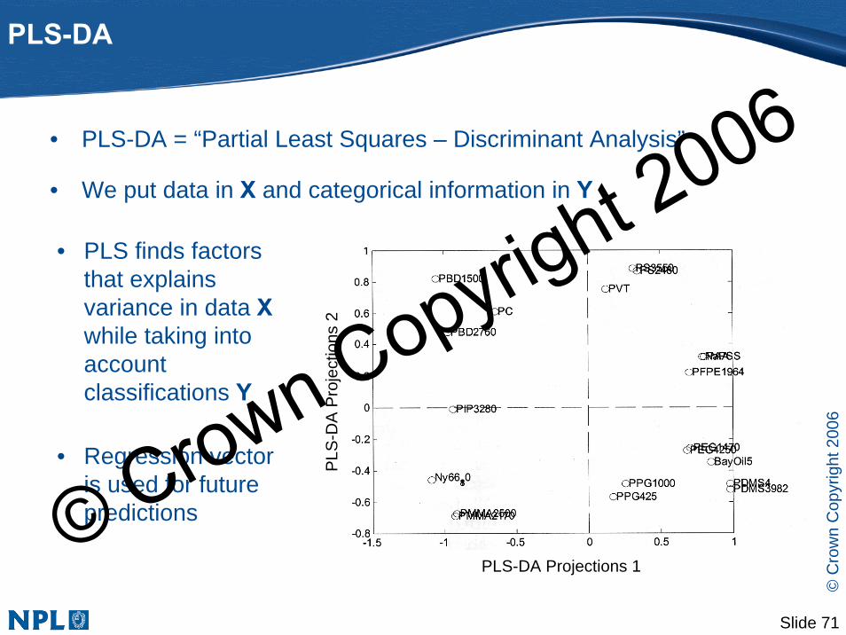
PLS-DA
• PLS-DA = “Partial Least Squares – Discriminant Analysis”
• We put data in X and categorical information in Y
PLS-DA Projections 1
PLS
-DA
Pro
ject
ions
2
• PLS finds factors that explains variance in data Xwhile taking into account classifications Y
• Regression vector is used for future predictions© Crown Copyright 2006
Slide 72
©C
row
n C
opyr
ight
200
6
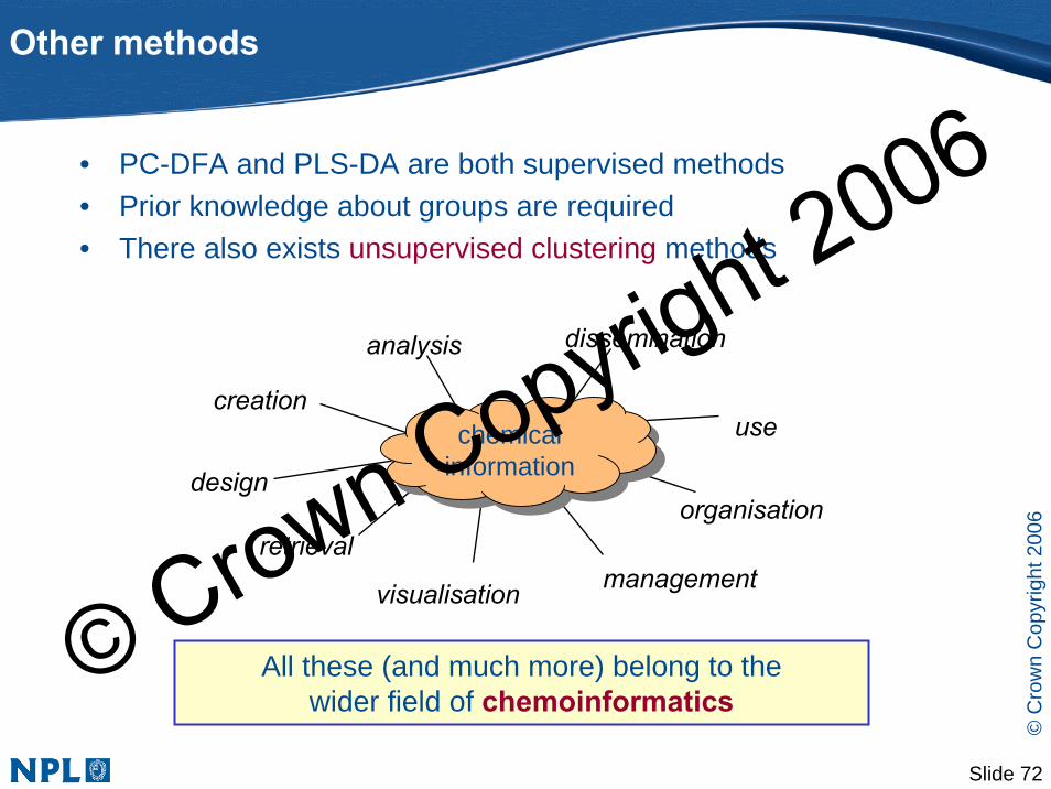
Other methods
• PC-DFA and PLS-DA are both supervised methods• Prior knowledge about groups are required• There also exists unsupervised clustering methods
design
retrieval
analysis dissemination
visualisation
usecreation
organisation
management
chemical informationchemical
information
All these (and much more) belong to thewider field of chemoinformatics
© Crown Copyright 2006

Slide 73
©C
row
n C
opyr
ight
200
6
Conclusion
In this tutorial we looked at– Identification using PCA and MCR– Quantification using MLR, PCR and PLS– Classification using PC-DFA, PLS-DA– Importance of validation for predictive models– Data preprocessing techniques and their effects– Matrix and vector algebra– New set of terminologies
Terms used here PCA MCR PLS
factors P loadings,
eigenvector, principal component
component spectra
latent vectors, latent variables
projections T scores component concentration scores
© Crown Copyright 2006

Slide 74
©C
row
n C
opyr
ight
200
6
Bibliography
General• A. R. Leach, V. J. Gillet, An introduction to Chemoinformatics, Kluwer Academic Publishers (2003)• S. Wold, Chemometrics; what do we mean with it, and what do we want from it?, Chemom. Intell. Lab. Syst. 30
(1995) 109• E. R. Malinowski, Factor analysis in Chemistry, John Wiley and Sons (2002)• P. Geladi, H. Grahn, Multivariate image analysis, John Wiley and Sons (1996)• D. J. Graham, NESAC/BIO ToF-SIMS MVA web resource, http://nb.engr.washington.edu/nb-sims-resource/
PCA• D. J. Graham, M. S. Wagner, D. G. Castner, Information from complexity: challenges of ToF-SIMS data
interpretation, Appl. Surf. Sci. 252 (2006) 6860• M. R. Keenan, P. G. Kotula, Accounting for Poisson noise in the multivariate analysis of ToF-SIMS spectrum
images, Surf. Interface Anal. 36 (2004) 203
MCR• N. B. Gallagher, J. M. Shaver, E. B. Martin, J. Morris, B. M. Wise, W. Windig, Curve resolution for multivariate
images with applications to TOF-SIMS and Raman, Chemom. Intell. Lab. Syst. 73 (2004) 105• J. A. Ohlhausen, M. R. Keenan, P. G. Koulta, D. E. Peebles, Multivariate statistical analysis of time-of-flight
secondary ion mass spectrometry using AXSIA, Appl. Surf. Sci. 231-232 (2004) 230• R. Tauler, A. de Juan, MCR-ALS Graphic User Friendly Interface, http://www.ub.es/gesq/mcr/mcr.htm
PLS• P. Geladi, B. Kowalski, Partial Least-Squares Regression: A Tutorial, Analytica Chimica Acta 185 (1986) 1• A. M. C. Davies, T. Fearn, Back to basics: observing PLS, Spectroscopy Europe 17 (2005) 28
© Crown Copyright 2006

Slide 75
©C
row
n C
opyr
ight
200
6
Acknowledgements
The work is supported by UK Department of Trade and Industry’s Valid Analytical Measurements (VAM) Programme and co-funded by UK MNT Network
For further information of Surface andNanoanalysis at NPL please visithttp://www.npl.co.uk/nanoanalysis
We would like to thank Dr Ian Fletcher (ICI Measurement Sciences Group) for images and expert analysis, and Dr Martin Seah (NPL) for helpful comments
© Crown Copyright 2006