Estimated PDFs of climate system properties including natural and anthropogenic forcings

and implications for 21st century climate change predictions.

Dr. Chris E. ForestMIT Joint Program on the

Science and Policy of Global Changehttp://web.mit.edu/globalchange/www/

Presentation to: Climate Decision Making Center Seminar Series

Carnegie Mellon University http://cdmc.epp.cmu.edu/SEMINARS.htm

April 24, 2006

Calibrated Climate Model Results

• Observed climate changes provide constraints on climate response to forcings.

• Forest et al. (2006) use observed climate changes to place probabilistic bounds on parameters in the IGSM climate component

• These constraints provide bounds for climate system response to any scenario of future climate forcings and help provide information for decision making process.

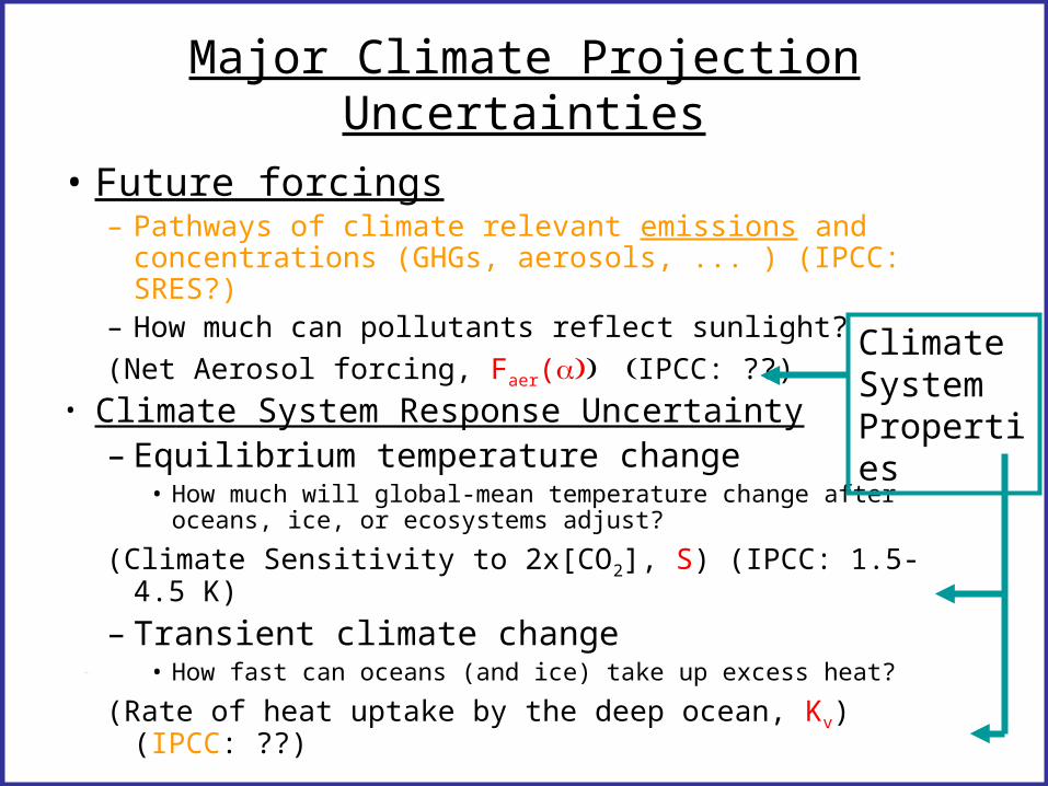
• Future forcings– Pathways of climate relevant emissions and

concentrations (GHGs, aerosols, ... ) (IPCC: SRES?)– How much can pollutants reflect sunlight?

(Net Aerosol forcing, Faer(IPCC: ??)• Climate System Response Uncertainty

– Equilibrium temperature change • How much will global-mean temperature change after

oceans, ice, or ecosystems adjust?

(Climate Sensitivity to 2x[CO2], S) (IPCC: 1.5-4.5 K)

– Transient climate change• How fast can oceans (and ice) take up excess heat?

(Rate of heat uptake by the deep ocean, Kv) (IPCC: ??)

Major Climate Projection Uncertainties

Climate System Properties

Estimating Uncertainty in Climate System Properties: p(S,Kv,FaerTobs)

1. Simulate 20th century climate using anthropogenic and natural forcings while systematically varying the choices of climate system properties: S, Kv, and Faer

2. Compare each model response against observed T

as in optimal fingerprint detection algorithm

3. Compare goodness-of-fit statistics to estimate

p(S,Kv,FaerTobs) for individual T diagnostics

4. Estimate p(S,Kv,FaerTobs) for multiple diagnostics

and combine results using Bayes’ Theorem

From: Forest et al. (2002), Science

Climate-change diagnostics (Ti)

1)Upper-air temperature changes, latitude-height pattern, [1986-1995] - [1961-1980] (Parker et al. 1997) (M=36x8)

2)Deep-ocean temperature trend, global, 0-3km (1952-1995) (Levitus et al. 2000, 2005) (M=1)

3)Surface temperature change, latitude-time pattern, (1946-1995 decadal means, 1906-1995 climatology, 4 zonal bands) (updated from Jones, 1994) (M=4 x 5)

Calculations with GSO forcings

Summary of Changes from GSO GSOL SV

• Updated Forcings for 1860-2001– Updated Greenhouse Gas concentrations – Updated Sulfur emissions from 1990-2001– Updated Ozone concentrations– Added Land-use Vegetation Changes– Added Volcanic and Solar forcings

• Updated climate model to 4o resolution and included new sea-ice model

• T Diagnostics identical to GSO

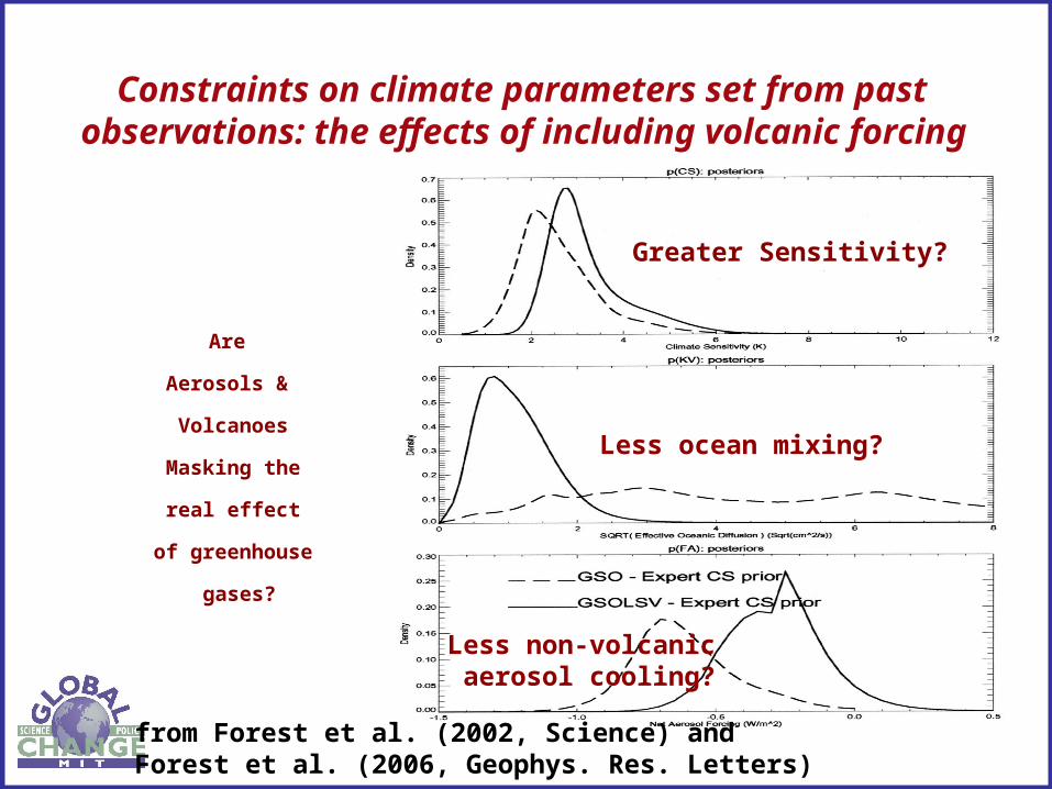
Constraints on climate parameters set from past observations: the effects of including volcanic forcing

Are

Aerosols &

Volcanoes

Masking the

real effect

of greenhouse

gases?

Greater Sensitivity?

Less ocean mixing?

Less non-volcanic aerosol cooling?

from Forest et al. (2002, Science) andForest et al. (2006, Geophys. Res. Letters)

Slow Sea level rise Fast

Probability Distribution for Climate Sensitivity and Rate of Deep-ocean heat uptake

Cluster of AOGCMs(Sokolov et al., 2003)

from Forest et al. (2006, GRL)

Implication:

Models overestimate rate of ocean heat uptake for transient response leading to faster adjustment to climate forcings.

Rejected

Accepted

90%

99%

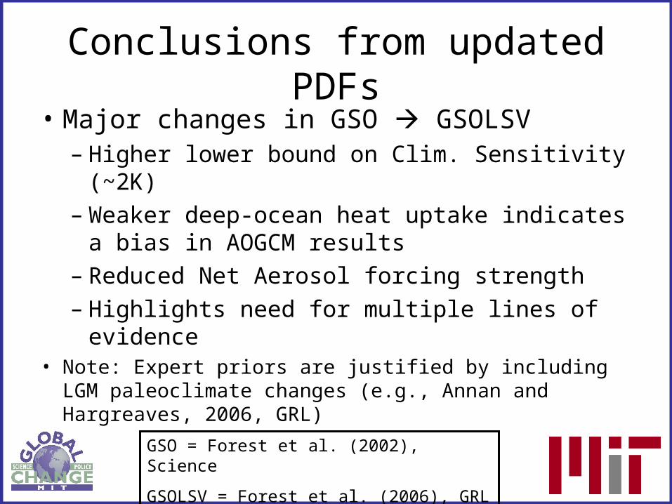
Conclusions from updated PDFs

• Major changes in GSO GSOLSV– Higher lower bound on Clim. Sensitivity (~2K)– Weaker deep-ocean heat uptake indicates a

bias in AOGCM results– Reduced Net Aerosol forcing strength – Highlights need for multiple lines of evidence

• Note: Expert priors are justified by including LGM paleoclimate changes (e.g., Annan and Hargreaves, 2006, GRL)

GSO = Forest et al. (2002), Science

GSOLSV = Forest et al. (2006), GRL

Deep-Ocean Temperature Data

• Higher coverage in NH than SH

• Still poor coverage in SH for surface

• Two alternatives to using Global estimate– Delete SH data and use trend in NH alone– Treat hemispheres separately as independent

diagnostics

Ocean Temperature Observations at 1km depth for two 5-yr periods: 1990-1994 (top) 1955-1959 (bottom)(from Levitus et al. (2005) Auxiliary Material)

Zdepth=1km, 1990-1994

Zdepth=1km, 1990-1994

Effects of missing data for ocean heat content anomaly estimates (HC)

Test two assumptions for values at missing data points: 1. HC = 02. HC = representative average

If existing data are a good representation of missing data, the change in heat content would have been larger.

From Gregory et al., GRL, VOL. 31, L15312, doi:10.1029/2004GL020258, 2004

Observed Tocean issues

• Without a detailed analysis, there is no clear guide for deleting estimates from Southern Hemisphere although data are sparse. A judgment call is required.

• Appears to be equal justification for using global or NH ocean temperatures. – Natural variability estimated by AOGCMs in NH is

much larger leading to weaker constraints.

• No change in mode indicates AOGCMs’ distribution is still biased.

Implications for future

• Two sensitivity tests– Effect of reduced oceanic heat uptake (OHU)

• Three runs with different Kv

Mode Kv = 0.64 cm2/s

2x OHU Kv = 2.56 cm2/s

~4x OHU = old mode Kv = 9.2 cm2/s

– Additional volcanic forcing for 21st century• Repeated past 50 yrs twice• Added past 100 yrs

Simulations by MIT IGSM2 (Sokolov et al., 2005) with reference emissions scenario from MIT EPPA4 (Paltzev et al., 2005). [ S= 2.9 K, Faer= -0.5 W/m2 ]

Implications for future climate change

• These features indicate that the reduction in the ocean heat content has a much larger effect on temperature changes than the volcanic forcing scenario.

• In terms of temperature changes from the present, the inclusion of the volcanic forcing appears to reduce temperature increase only by at most ~0.5 oC while reducing Kv leads to an increase of ~1.8 oC by 2100 with S = 2.9 oC and Faer = -0.5 W/m2 for this reference emissions scenario.