essays on adaptation responses to climate variability in india
TRANSCRIPT

The Pennsylvania State University
The Graduate School
Department of Agricultural Economics, Sociology & Education, and Demography
ESSAYS ON ADAPTATION RESPONSES TO CLIMATE VARIABILITY IN INDIA
A Dissertation in
Agricultural, Environmental & Regional Economics and Demography
by
Esha D. Zaveri
© 2016 Esha D. Zaveri
Submitted in Partial Fulfillment
of the Requirements
for the Degree of
Doctor of Philosophy
August 2016

ii
The dissertation of Esha D. Zaveri was reviewed and approved* by the following:
Karen Fisher-Vanden
Professor of Environmental and Resource Economics
Graduate Program Director
Dissertation Adviser
Co-Chair of Committee
David Abler
Professor of Agricultural, Environmental & Regional Economics and Demography
Co-Chair of Committee
Jenni Evans
Professor of Meteorology
Douglas H. Wrenn
Assistant Professor of Environmental and Resource Economics
*Signatures are on file in the Graduate School
iii
ABSTRACT
Studying interactions between human and natural systems presents a unique opportunity
for multidisciplinary and policy-relevant research. This dissertation consists of three chapters
that examine how changes in water access, availability and use influence agricultural adaptation,
and labor mobility in rural India. Since an increasingly variable future climate will amplify
stresses on the water cycle, with large and uneven consequences1, the findings from these
chapters have important implications for both environmental and developmental policies that
seek to promote long-run sustainability.
The focus on India is deliberate. India is the world’s largest agricultural water and
groundwater user and is thus likely to be particularly vulnerable to future changes in climate.
Water, especially groundwater, has played a fundamental role in shaping the course of agrarian
change and development in India. Groundwater access is salient to the livelihoods of 263 million
agricultural laborers and small-scale farmers, who farm on less than two hectares of farmland
and comprise three fifth of the country’s poor. However, at the same time, parts of the country
are already experiencing falls in groundwater levels, and the current drought has further
magnified India’s vulnerability to water stress.2
The first chapter assesses the complex challenges of groundwater depletion, surface water
stress, and food security that India is likely to face with future climate change. It provides the
first multi-model assessment of the extent of non-renewable groundwater use in India by mid-
century, its importance in sustaining food production, and the role that government adaptation
through investments in large infrastructure projects might play in decreasing India’s dependence
on non-renewable groundwater in the future. Since it combines an econometric model of
irrigation decision-making with a process based hydrology model, it explicitly accounts for both
groundwater demand and supply. Results from the panel-based econometric model highlight the
fundamental role that inter-annual variations in the monsoon play in driving irrigation decisions
1 World Bank (2016) “High and Dry: Climate Change, Water and the Economy”
2 “India’s Water Crisis” New York Times, May 3, 2016 ; Vidhi Doshi, “India's drought migrants head to cities in
desperate search for water”, The Guardian, April 27, 2016; Amit Anand Choudhary, “Over 25% of India’s
population hit by drought, Centre tells Supreme Court”, The Times of India, Apr 20, 2016
iv
across crops and seasons. The estimated coefficients from the econometric model are used to
make projections of irrigated area changes under five different climate future scenarios up to
2050, which are coupled with the physical hydrologic cycle to assess the sustainability of
groundwater demand and how groundwater levels are likely to change. The results highlight
significant spatial and regional heterogeneity in future changes in groundwater demand and
supply. We find that even in areas that experience projected increases in precipitation,
groundwater levels will continue to drop over the next 50 years as a result of an expansion of
irrigated agriculture, and a complete loss of non-renewable groundwater irrigation could reduce
annual crop production by as much as 25 percent, directly affecting the caloric intake of more
than 170 million people. Results also indicate that India’s large proposed river linking scheme—
recently launched with the first river link between the Krishna and Godavari rivers on
September 16, 2015—which is intended to create a national water grid is unlikely to alleviate
groundwater stress nationally without substantial investments in reservoir storage capacity.
The second chapter examines how the introduction of high yield variety of seeds in the
mid-1960s (the Green Revolution) and the resulting path dependency of groundwater
development underlies the results we see in chapter one. It assesses the impact of different types
of water infrastructure and sheds light on the resulting behavior of end-users of water. In
particular, it investigates the role played by groundwater wells, tanks and dams in reducing the
uncertainty associated with increased monsoonal variability. Results show that access to
tubewells helps to dampen the impact of negative precipitation shocks on irrigation decisions
associated with wheat, a staple of India’s food supply, while upstream dams do not significantly
contribute to this dampening effect. In contrast, having access to dugwells exacerbates the
impact of a fall in monsoon precipitation curtailing irrigation of wheat. The results suggest that
increasing access to more reliable, yet largely unsustainable sources of groundwater have
equipped farmers with the ability to withstand monsoonal fluctuations in the irrigation-intensive
dry season. The results also indicate that initial groundwater endowments have influenced the
types of irrigation infrastructure and capacities that have developed in India as a result of the
Green Revolution, with lasting effects on the adaptability of agriculture to weather shocks.
The third chapter investigates how irrigation water access, availability and use also have
wider spillover effects on the agrarian labor economy. Using nationally representative

v
household-level survey data combined with location specific weather, irrigation, groundwater
and electricity data, it examines short-term migration, a common and economically important
mechanism by which rural households diversify their income sources. Results show that
migration decisions respond to agricultural opportunity costs associated with irrigation and that
access to assured irrigation determines the relative benefits of migration. Tubewells, especially
deep tubewells, allow farmers and laborers to farm lands even in times of rainfall scarcity and
this benefit lowers the degree of temporary migration. Moreover, results also indicate that the
likelihood of temporary migration decreases from regions which consistently face deeper
groundwater levels as long as electricity distribution is more developed in these areas. This
suggests that an increase in electrification facilitates the use of electric pumps for groundwater
extraction and enables farmers to adapt or invest in technology that allows groundwater to be
pumped from even greater depths. Therefore, better access to the benefits of groundwater
through higher electricity provision increases the agricultural focus of rural individuals, and
significantly decreases short-term migration. Since short-term migration is primarily an income
smoothing strategy used to diversify risk in the presence of agricultural productivity shocks, our
findings suggest that maintaining access to groundwater is an important lever for sustaining rural
livelihoods.

vi
TABLE OF CONTENTS
LIST OF TABLES .......................................................................................................................... ix
LIST OF FIGURES ......................................................................................................................... x
ACKNOWLEDGEMENT .............................................................................................................. xi
Chapter 1 ......................................................................................................................................... 1
Adaptability of Irrigation to a Changing Monsoon in India: How far can we go? ......................... 1
Abstract ........................................................................................................................................... 1
1.1 Introduction ............................................................................................................................... 2
1.2 Data and Study Region ............................................................................................................. 9
1.2.1 Context: The Indian Monsoon............................................................................................ 9
1.2.2 Agricultural Data .............................................................................................................. 10
1.2.4 Summary Statistics ........................................................................................................... 13
1.3. Econometric Model ................................................................................................................ 13
1.3.1 Residual Variation in Weather ......................................................................................... 17
1.4 Results ..................................................................................................................................... 17
1.5 Robustness Checks.................................................................................................................. 19
1.6 Climate Change Impacts on Unsustainable Groundwater Demand ........................................ 21
1.6.1 Projections ........................................................................................................................ 21
1.6.2 Coupling with Physical Hydrologic Cycle ....................................................................... 24
1. 7 Policy Implications ................................................................................................................ 25
1.7.1 Loss of Unsustainable Groundwater Demand and Food Production ............................... 25
1.7.2 National River Linking Project and Inter-Basin Transfers .............................................. 27
1.8 Conclusion .............................................................................................................................. 29
References ..................................................................................................................................... 31
Figures........................................................................................................................................... 39
Tables ............................................................................................................................................ 46
Appendix ....................................................................................................................................... 55
Chapter 2 ....................................................................................................................................... 59
Water in the Balance: The Impact of Water Infrastructure on Agricultural Adaptation to Rainfall
Shocks in India .............................................................................................................................. 59

vii
2.1 Introduction ............................................................................................................................. 60
2.2 Data ......................................................................................................................................... 62
2.2.1 Aquifers ............................................................................................................................ 62
2.2.2 Sources of Irrigation and Electricity ................................................................................ 62
2.3 Path-dependency of Groundwater Development .................................................................... 64
2.4 Background: Groundwater Technology and Electricity ......................................................... 66
2.5 Heterogeneous Effects ............................................................................................................ 68
2.5.1 Empirical Model and Results ........................................................................................... 68
2.5 Conclusion .............................................................................................................................. 70
References ..................................................................................................................................... 71
Figures........................................................................................................................................... 73
Tables ............................................................................................................................................ 78
Chapter 3 ....................................................................................................................................... 80
The Impact of Water Access on Short-term Migration in Rural India ......................................... 80
3.1 Introduction ............................................................................................................................. 81
3.2 Conceptual Framework ........................................................................................................... 86
3.3 Data and Context..................................................................................................................... 92
3.3.1 National Sample Survey (NSS) Migration Data .............................................................. 92
3.3.2 Irrigation Data .................................................................................................................. 94
3.3.3 Electricity Data ................................................................................................................. 95
3.3.4 Groundwater Level Data .................................................................................................. 97
3.3.5 Groundwater Levels and Electricity Access .................................................................... 97
3.4 Empirical Approach and Results: ......................................................................................... 100
3.4.1 Impact of Irrigation Technology and Rainfall Shocks ................................................... 102
3.4.2 Impact of Groundwater Levels and Electricity .............................................................. 104
3.4.4 Seasonal, Demographic and Household Characteristics: ............................................... 105
3.5 Robustness Checks................................................................................................................ 107
3.6 Conclusion ............................................................................................................................ 109
References ................................................................................................................................... 111

viii
Figures......................................................................................................................................... 118
Tables .......................................................................................................................................... 124
Appendix ..................................................................................................................................... 138

ix
LIST OF TABLES
Table 1.1a. Summary Statistics 1970-2005 .................................................................................. 46
Table 1.1b. Percent net irrigated area to net sown area ................................................................ 46
Table 1.2: Residual variation in weather ...................................................................................... 47
Table 1.3: The Impact of the Monsoon on Wet Season (Kharif) Irrigated Areas ........................ 48
Table 1.4: The Impact of the Monsoon on Dry Season (Rabi) Irrigated Areas ............................ 49
Table 1.5: Robustness Checks: Wet Season (Kharif) Irrigated Areas .......................................... 50
Table 1.6: Robustness Checks: Dry Season (Rabi) Irrigated Areas ............................................. 51
Table 1.7: Robustness Checks: Rice Irrigated Areas .................................................................... 52
Table 1.8: Robustness Checks: Standardized Weather Variables ................................................ 53
Table 1.9: The Impact of Unsustainable Groundwater on Irrigated Agriculture and Food Supply
....................................................................................................................................................... 54
Table 2.1. Log Wheat Irrigated Area: Aquifer Capacity .............................................................. 78
Table 2.2. Log Wheat Irrigated Area: Heterogeneous Effects ...................................................... 79
Table 3.1. Short-term Migrants (STMs) ..................................................................................... 124
Table 3.2. Summary Statistics .................................................................................................... 125
Table 3.2. Summary Statistics (continued) ................................................................................. 126
Table 3.3. Likelihood of short-term migration in response to irrigation .................................... 127
Table 3.4. Likelihood of short-term migration in response to the type of irrigation .................. 128
Table 3.5. Likelihood of short-term migration in response to groundwater levels and electricity
provision ..................................................................................................................................... 129
Table 3.6. Likelihood of short-term migration in response to groundwater levels and electricity
provision (Night lights) ............................................................................................................... 130
Table 3.7. Robustness Checks: Likelihood of short-term migration in response to irrigation
(Probit) ........................................................................................................................................ 131
Table 3.8. Robustness Checks: Likelihood of short-term migration in response to groundwater
levels and electricity provision (Probit) ...................................................................................... 132
Table 3.9a. Robustness Checks: NREGS and likelihood of short-term migration in response to
irrigation ...................................................................................................................................... 133
Table 3.9b. Robustness Checks: NREGS and likelihood of short-term migration in response to
groundwater levels and electricity provision .............................................................................. 134
Table 3.10a. Robustness Checks: Household decisions, short-term migration in response to
irrigation (Poisson)...................................................................................................................... 135
Table 3.10b. Robustness Checks: Household decisions, short-term migration in response to
groundwater levels and electricity provision (Poisson) .............................................................. 136
Table 3.11. Robustness Checks: Likelihood of short-term migration in response to groundwater
levels and electricity provision (Nightlights 2006) ..................................................................... 137

x
LIST OF FIGURES
Fig. 1.1: Aggregate Changes in Wheat and Rice Area, Irrigation and Production ....................... 39
Fig. 1.2. Coupled Human and Physical System Model Schematic ............................................... 39
Fig. 1.3a: Average Historical Monsoon Rainfall and No. of Rainy Days (June-September) ....... 40
Fig. 1.3b: Historical Inter-annual and Inter-decadal Variability in Monsoon Rainfall (June-
September) .................................................................................................................................... 40
Fig. 1.4: Future changes in Monsoon Rainfall and No. of Rainy Days ........................................ 41
Fig. 1.5: Changes in Temperature over time................................................................................. 42
Fig. 1.6: Projections of Irrigated Area to 2050 ............................................................................. 42
Fig. 1.7: Trends in Groundwater Levels between 1979-2000 and 2029-2050 ............................. 43
Fig. 1.8: Volume of Unmet Irrigation Water Demand in Absence of Unsustainable Groundwater
....................................................................................................................................................... 44
Fig. 1.9: Crop Production (million tons) Dependent on Unsustainable Groundwater.................. 44
Fig 1.10: National River Linking Project and Unsustainable Groundwater ................................. 45
Fig. A.1.1: Aggregate Changes in Well and Surface Based Irrigation ......................................... 55
Fig. A.1.2: Distribution of Irrigated Area ..................................................................................... 56
Fig. A.1.3: Projections of Crop Irrigated Area to 2050 ................................................................ 57
Fig. A.1.4: Trends in Groundwater Levels between 1979-2000 and 2029-2050 from five GCMs
....................................................................................................................................................... 58
Fig 2.1 Aquifer capacity in northern India.................................................................................... 73
Fig 2.2 Trends in area under High Yielding Varieties (HYV) ..................................................... 74
Fig 2.3: Trends in irrigated area by different sources ................................................................... 74
Fig 2.4: Differential trends in area under High Yielding Varieties ( HYV) by aquifer capacity . 75
....................................................................................................................................................... 75
Fig 2.5: Differential trends in tubewell irrigated area by aquifer capacity ................................... 75
Fig 2.6: Differential trends in dugwell irrigated area by aquifer capacity .................................... 76
Fig 2.7: Trends in electrification ................................................................................................... 76
Fig 2.8: Differential trends in electrification by aquifer capacity ................................................. 77
Fig. 3.1: Short-term migration .................................................................................................... 118
Fig. 3.2: Spatial distribution of electricity provision .................................................................. 119
Fig. 3.3: Percentage of villages according to depth to groundwater ........................................... 120
Fig. 3.4: Percentage of groundwater structures .......................................................................... 120
Fig. 3.5 Categorization of districts according to depth to groundwater ...................................... 121
Fig. 3.6 Coefficient estimates for household and individual characteristics .............................. 122
Fig. 3.7 Coefficient estimates for individual employment status ............................................... 122
Fig. 3.8 Short-term migrants by age and sex .............................................................................. 123

xi
ACKNOWLEDGEMENT
Begin at the beginning and go on till you come to the end: then stop.
– Lewis Carrol
This dissertation represents a culmination of a journey that would not have been possible
without the help of many people.
I want to thank my adviser Karen Fisher-Vanden for giving me the freedom to pave my
own path, for anchoring my efforts, and for her exceptional support, and encouragement to learn
and grow as a researcher. I am thankful to my co-adviser David Abler for his profound
scholarship, valuable feedback and guidance, and for shaping my thinking. I am grateful to my
committee members- Douglas Wrenn for his phenomenal empirical rigor and super brain power
in guiding me, and whose lessons in econometrics and writing have motivated me to think
incisively and Jenni Evans for pointing me to literature on the monsoon in India, and inspiring
me to strive for intellectual rigor. I am grateful to Danielle Grogan, doctoral student in hydrology
at the University of New Hampshire, without whose unstinting support, collaboration and
friendship this project would not have been possible. I am thankful to the Department of
Agricultural, Economics, Sociology and Education, the National Science Foundation, Water
Sustainability and Climate program (EAR-1038614), the U.S. Department of Energy, Office of
Science, Biological and Environmental Research Program, Integrated Assessment Program (DE-
SC0005171) and the National Science Foundation’s Sustainable Research Network program
(cooperative agreement GEO-1240507) for supporting my research.
I am thankful to all my wonderful professors and mentors at Penn State. Ted Jaenicke’s
kindness, and faith in me as I transitioned into Penn State has been invaluable, and Spiro
Stefanou’s many spoken and unspoken words of support helped me navigate what seemed like
insurmountable mountains of doubt. I am grateful to James Shortle and Stephen Matthews, who
marked critical inflection points in my thinking. James Shortle’s course in environmental and
resource economics triggered my interest in spatial externalities related to groundwater
movements. Stephen Matthews’s spatial demography classes were a source of great joy and
introduced me to the beauty of cartography, and thinking spatially.
I am indebted to S. Chandrasekhar at the Indira Gandhi Institute for Development
Research in Mumbai for his valuable support during my data gathering visits to India, and
answering countless questions about NSS data. I am grateful to Tushar Shah, Yashree Mehta,

xii
and Shilp Verma at the International Water Management Institute for hosting me on my visit to
Anand, Gujarat, and for insightful discussions about data and policy on the field. I thank G.
Sharma, S.K.Singh, and A. Gupta at the Central Groundwater Board, Faridabad, and the Ministry
of Water Resources, New Delhi for sharing data and providing contextual information. I am
thankful to Aditi Mukherji, Stuti Rawat, Chinmay Tumbe and Juan Pablo Rud for sharing data
and answering my questions. I am grateful to the International Institute for Population Studies in
Mumbai for allowing me to use their library resources. I am thankful to Yosef Bodovski at Penn
State’s Population Research Institute for his generous help with my GIS related queries, Badri
Narayanan for helpful insights about research and Seema Kapur for knocking on ministerial
doors in Faridabad. I thank Robert Nicholas for sharing weather data, and relevant information
about climate data sources, and Chandra Kiran Krishnamurthy for valuable insights about Indian
weather station data early on in my research.
My home away from home in State College, Nalini Krishnankutty and Sounder Kumara,
have been there for me through thick and thin. Thank you for the countless goodies, incredible
support, love, care and warmth. Thanks to my music family, and guru, Arijit Mahalanabis, for
expanding my musical horizons, and giving my creative side free reign to flourish, explore and
dream alongside the PhD.
Many friends in State College have contributed to my PhD journey immeasurably and
enriched my graduate school experience. Shonel Sen, Daniela Puggionni, Meri Davlasheridze,
Milagro Saborio Rodriguez, Qin Fan, Nikolaos Mykoniatis, Monica Roa, Jing Li, Julia
Morasteanu, Iryna Demko, Yeris Mayol Garcia, Susana Quiros, Lucia Tabacu, Sakshi Bhargava,
Deepak Iyer, Tushar Shanker, Rucha Modak, Sayali Phadke, Kishan Patel, Anne Parson,
Beatrice Abiero, and others have humored me, advised me at many junctures, provided
intellectual and moral support over gallons of chai, laughter and tears. Murali Haran reminded
me to look beyond the trees to the forest, and provided sound advice whenever I needed it.
Above all, I value the love and unwavering support of my parents, my grandmother, my
sister and my extended family- my go-to uncle, rock and anchor Jay Madan; the precious care of
Aparna Zaveri and Prashant Kapoor; my loving Charu Shah and Vipul Shah. They have helped
me ascend hills, supported me through days of frenetic worry, enthusiastically cheered me on,
and answered countless telephone calls at midnight. Without their inspiration, good judgement
and faith, I would not have made it this far.

xiii
DEDICATION
To my parents
-Sonal and Dilip Zaveri-
who instilled in me a love for learning

1
Chapter 1
Adaptability of Irrigation to a Changing Monsoon in India: How far can we go?3
Abstract: Given historical uncertainties surrounding the timing, magnitude, and coverage of the
Indian monsoon, farmers have exploited deep groundwater as a reliable source of irrigation in
India over the past forty years. However, current rates of groundwater pumping in India threaten
to push groundwater levels out of the reach of millions of farmers. Moreover, there is a great
deal of uncertainty surrounding both the future availability of water, as a result of climate change,
and how the agricultural sector will respond. Past econometric studies that estimate the impacts
of climate change on agriculture do not simultaneously take account of and assess changes in
water supplies. In this paper, we fill this gap by combining an econometric model of irrigation
decision-making with irrigation water availability by explicitly accounting for both groundwater
demand and supply. Using district-level panel data from 1970-2005, we find that inter-annual
variation in the monsoon plays a fundamental role in driving irrigation decisions across crops
and seasons. We use our panel-based parameter estimates to make projections of irrigated area
changes under five different climate future scenarios up to 2050, which are coupled with the
physical hydrologic cycle to assess the sustainability of groundwater demand and how
groundwater levels are likely to change. We find that even in areas that experience projected
increases in monsoonal rainfall, expansion of irrigated agriculture will lead to continued declines
in groundwater levels. We also show that without groundwater-based irrigation, dry-season crop
production could be reduced by as much as 50 percent, which represents the caloric intake of
more than 170 million people. We also find that the ability of India’s large National River
Linking Project (NRLP) to alleviate groundwater stress will depend heavily on concurrently
increasing reservoir storage capacity.
Keywords: Groundwater, Climate change, Indian monsoon, Food security, Inter-basin water
transfers
JEL Codes: O13, Q15, Q25, Q54, Q56
3 This work is in collaboration with Danielle Grogan, Steve Frolking and Richard Lammers at the Institute for Earth,
Oceans and Space at University of New Hampshire

2
1.1 Introduction
“Every cloud in the sky is watched, every symptom of rain checks irrigation…”
- The Calcutta Review, Volume 12, 1849
Like many developing countries, agriculture plays a significant role in India's social and
political economy. While most of India’s agriculture is small scale in nature, in total it accounts
for more than a fifth of India’s GDP and is one of the country’s largest employers. Moreover, the
agriculture sector is the primary food supplier for India’s 1.2 billion people. India is also one of
the largest agricultural producers in the world exporting around $39 billion in raw agricultural
products and over 4.4 million tons of milled rice annually (Ministry of Agriculture, 2014). Thus,
given the size and importance of India’s agriculture sector and the fact that many of its key
inputs depend on weather and climate outcomes, it is not surprising that it is viewed as
particularly vulnerable to predicted future changes in climate. (Mendelsohn et al., 2006;
UNFCCC, 2007).
Much of the success of India’s agriculture sector is directly linked to the timing and
intensity of the summer monsoon, an annual weather phenomenon arriving around June and
lasting through the end of September, which brings rain to the Indian subcontinent. While every
monsoon season brings some rain, there is always a great deal of uncertainty surrounding the
overall magnitude, timing, and spatial and temporal coverage of each monsoonal event. Thus,
millions of farmers, who depend on agriculture for their livelihood, wait in anticipation every
year for the monsoon’s ultimate outcome with changes in precipitation patterns directly
impacting water availability and the productivity of agriculture. 4
Indian agricultural productivity and food security is also significantly impacted by
irrigation. Irrigated crop productivity is generally found to be higher than rain-fed crop
productivity (Fischer et al, 2007; Bruinsma , 2009), and for decades the Indian government’s
policies have promoted irrigation expansion as a method for improving agricultural growth,
smoothing production risk, and alleviating rural poverty (Shah, 2010). These benefits, however,
have come at the cost of increased pressure on many irrigation water sources with irrigation
accounting for 80-90 percent of India’s water demand (Wada et al., 2013; Shah, 2013).
4 India's farmers pray for rain, Kazmin (2012) in Financial Times, July 25, 2012. The timing of the onset of the
monsoon (the first phase of the monsoon) is said to be an important aspect for agricultural profits (Rosenzweig and
Binswanger, 1993).

3
Moreover, predicted future changes in climate further complicate the situation by adding
additional uncertainty about future water availability (supply) (Ferguson and Gleeson, 2012;
Taylor et al., 2013).5 Thus, to fully understand the implications of climate change and how it is
likely to impact agriculture in India, it is necessary for researchers and policymakers to have
models that account for both the demand for and supply of different sources of water and how
these will interact under different climate scenarios. To examine how climate variability is likely
to influence irrigation water use in India, this study uses a coupled modeling approach that
combines models of both behavioral irrigation decision-making and the physical-hydrologic
water cycle. This multi-model approach is necessary as it enables us to assess both water demand,
via changes in irrigation and cropping decisions, and water supply, through sustainable sources
supplied by groundwater recharge, surface rivers, and reservoirs and through unsustainable
sources supplied by groundwater extraction in excess of recharge (Grogan et al., 2015).
Groundwater is the most prominent and important source of irrigation in India as it
reduces uncertainty and increases productivity by providing reliable and timely delivery of water
during critical periods of crop growth and moisture stress (Sekhri 2011; Shah, 2010). In contrast,
public provision of irrigation via surface-water sources generally suffers from chronic
underperformance and has a chequered history (Shah, 2010). Beginning in the 1960s, with the
onset of the Green Revolution and the introduction of high yielding variety (HYV) crops, India
saw a significant increase in groundwater irrigation (Appendix, Fig.1.1) and is currently the
world's largest user of groundwater (Shah, 2010).6 This increase was primarily driven by the
emergence of atomistic or personal irrigation systems and the use of subsidized power to pump
groundwater from individual tube wells (Shah, 2010).7 Through this process, approximately 90
million rural households have come to directly depend on groundwater irrigation (NSSO, 2014).
Between 1970 and 2004, while overall crop area for staple crops like rice and wheat remained
fairly stable, irrigated area saw a rapid increase (Fig.1.1) with groundwater extractions
5 According to the 2007 IPCC Report: “Of all sectoral water demands, the irrigation sector will be affected most
strongly by climate change….” 6 This is in contrast to state-controlled canal-based irrigation that was prevalent from the early 1800s to 1970 (Shah,
2011; Shah, 2010). Prior to the Green Revolution, India was, in fact, a major agricultural importer, and policy
discourse at the time revolved around whether to focus on developing HYV crops at home or import from other
countries. For more discussion on this, see Abler et al. (1994). 7 “The State has assumed the authority for the design, construction and operation of all major projects for
exploitation of surface water….the exploitation of groundwater is left to the private sector” (Vaidyanathan, 2010, p
14)

4
accounting for 70-80 percent of the value of agricultural production (World Bank, 1998). This
underscores the important role that groundwater irrigation has played in supporting upward
trends in yields and productivity.
Increased use of groundwater irrigation has led to widespread over-extraction of
groundwater resources, which is unsustainable in the long term (Aeschbach-Hertig and Gleeson,
2012).8 Since 1980, groundwater levels have dropped from 8 meters below ground level (mbgl)
to 16 mbgl in northwestern India and from 1 to 8 mbgl in the rest of the country (Sekhri, 2012).
Northwestern India lost 109 km3 of groundwater between 2002 and 2008 (Rodell, Velicogna and
Famiglietti, 2009), which is an order of magnitude larger than the groundwater depletion
experienced by California’s Central Valley during the same period (Famiglietti et al., 2011), and
twice the volume of India’s largest surface water reservoir (Rodell, Velicogna and Famiglietti,
2009). Recent research has demonstrated that groundwater declines can lead to increases in
poverty and threaten food production – especially for rural households (Sekhri, 2013; Sekhri,
2014). Exploiting the exogenous variation in pump technology used by farmers to draw
groundwater, Sekhri (2014) finds that in areas where water tables are deeper, poverty rates are
10-12 percent higher than where groundwater is more easily accessible. Similarly, food grain
production can decline by 8percent in response to a 1 meter decline in groundwater below its
long-run mean (Sekhri, 2013). 9
This directly affects small-scale farmers who typically own less
than two hectares of farmland10
, control the majority of the landholdings in India, and produce
41 percent of India’s food grains (Singh, 2002). These farmers use groundwater to irrigate half
their land (either through their own wells or through informal groundwater markets) and are
likely to be the hardest hit by continued declines in groundwater. Consequently, the sustainable
use of groundwater in the future remains a serious concern as climate change, through its impact
on agriculture, is likely to add to their already high vulnerability.
India has a monsoonal climate with a wet (Kharif) season that receives up to one meter of
rainfall each year and a dry (Rabi) season in which rainfall is insufficient to grow most crops and
irrigation must be used. Irrigation based on groundwater sources enables farmers to both
8 India's groundwater crisis has been called 'anarchic': "When the balloon bursts, untold anarchy will be the lot of
rural India."(Shah, 2010) 9 Duflo and Pande (2007) find that surface water irrigation by dams raises production by only 0.34 percent and
actually increases poverty in upstream reaches in India. 10
In 2011 the average farm size in the United States was 234 acres or 94 hectares.

5
supplement water for crops in the wet season and sustain crops in the dry season.11
The ability to
irrigate without using unsustainable or over-extracted groundwater, however, is largely made
possible by the summer monsoon rainfall that replenishes rivers and reservoirs and is captured as
rechargeable groundwater. From these sustainable sources, farmers assess the supply of rain
during the monsoon season and the amount that gets captured and stored at the end of the season
in order to make decisions about increasing or decreasing irrigated areas for different crops
(Fishman, 2012). Previous research has shown that a significant link exists between annual
monsoon rainfall and irrigated area in India as farmers tend to respond to water scarcity along the
extensive margin by adjusting the extent of cultivated and irrigated area (Siegfried et al, 2010;
Fishman et al., 2011).12
Thus, any climatic changes that impact the outcome of the monsoon are
likely to have a direct impact on the cropping and irrigation decisions made by farmers.13
Previous hydrology studies have attempted to simulate joint future climate and irrigation
scenarios (Fischer et al., 2007; Wada et al., 2013; Hanasaki et al., 2013; Elliott et al., 2014).
These studies range from basin to global in scale and use a variety of different methods for
projecting irrigated area with most either assuming that current irrigated areas persist unchanged
into the future (Wada et al., 2013), using a fixed growth rate for irrigated area based on FAO
reports (Hanasaki et al., 2013), using an integrated assessment model to project changes in total
crop areas along with a fixed growth rate for irrigated area (Fischer et al., 2007), or altering
irrigated areas based on changing annual surface water supplies (Elliott et al., 2014). These
studies, however, do not account for the dynamic behavioral response of farmers’ irrigation
decisions in response to changing precipitation patterns, which have been emphasized in recent
econometric studies (Fishman et al., 2011; Fishman, 2012). While econometric studies are better
at modeling human behavior (demand), they do not account for biophysical supply constraints
implicitly assuming that water will be forthcoming for all irrigation demand. Thus, they cannot
11
The wet season coincides with the monsoon season, and the dry season immediately follows the wet season. 12
Other aspects of irrigated agriculture such as crop and cultivar switching are important potential adaptation
strategies that also influence irrigation water use. These aspects, however, are outside the scope of the study. 13
The future of monsoon rainfall continues to remain extremely uncertain, although historical evidence suggests that
the number of dry and wet spells have risen over the past fifty years (Singh et al., 2014). Some climate change
studies predict both an increase (Hu et al., 2000; Lal et al., 2001; Chaturvedi et al. 2012) and a suppression of
monsoon precipitation (Ashfaq et al., 2009) along with increases in inter-annual and intra-seasonal variation (Menon
et al., 2013) and increasing temperatures (Chaturvedi et al., 2012). Figures 1.4 and 1.5 show that the five future
climate scenarios chosen in this study reflect both increases and decreases in precipitation along with consistent
increases in temperatures. Such changes in the climate will impact irrigation water demand and supply due to farmer
irrigation decisions, water supply, and physiological crop water requirements

6
simultaneously model changes in both irrigation demand and changes in the water supplied to
meet those demands, which is particularly important for India where different irrigation water
sources have distinct implications for sustainability.
In this study, we combine an econometric model with a process-based hydrology model
(Fig. 1.2) to assess the relationship between climate change, irrigation decision-making, crop
water use and supply, and crop production in India. Given the uncertainty about future changes
in the Indian monsoon, we explore a range of possible scenarios using a suite of global
circulation models (GCMs) that represent both declines and increases in mean monsoon
precipitation (Fig 1.4). The combination of the econometric and hydrology models is critical,
both as a research tool and as a policymaking tool so that India can better plan for the future as
well as assess the role that adaptation responses and policy measures may play going forward.
One such policy initiative proposed by the Government of India is to move 178 billion m3yr
-1 of
water across river basin boundaries (Chellaney, 2011). Recently launched with the first river link
between the Krishna and Godavari rivers on September 16, 201514
, this National River Linking
Project (NRLP) has been proposed as a solution to groundwater stress by increasing irrigated
agriculture through surface irrigation and artificial groundwater recharge. Better understanding
of future irrigation water demand and availability, with emphasis on unsustainable groundwater
dependence, is needed to assess such policies and formulate effective strategies to adapt to
climate change.
In order to implement our econometric model and assess the impact of changes in
monsoon rainfall on irrigation outcomes, we combine detailed crop and weather data spanning
36 years (1970-2005) for all of the districts in the main agricultural states of India in which
farmers' behavioral aspects are embedded implicitly. The panel nature of our data allows us to
estimate the relationship between inter-annual variation in the monsoon and district-level
irrigation decisions for six major crops – rice, wheat, maize, sorghum, barley, and cotton – while
controlling for macro-level trends and district-level unobservables15
. Identification in our model
14
“Godavari, Krishna rivers formally linked in Andhra Pradesh”, Indian Express, September 16, 2015.
http://articles.economictimes.indiatimes.com/2015-09-16/news/66604493_1_krishna-delta-krishna-river-inter-
linking 15
Panel data methods, as used in this paper, do not account for long term adaptation, as cross-sectional studies do
(Mendelsohn, Nordhaus and Shaw, 1994; Sanghi, Mendelsohn and Dinar, 1998; Kumar and Parikh, 2001;
Kurukulasuriya, Kala and Mendelsohn, 2011), and only capture short- term adaptation exploiting year-to-year
variability in weather outcomes. Focus on explicitly understanding medium-term and long-term adaptation has
started to emerge. Taraz (2015)'s study on farmer crop choices and irrigation investment in response to climate

7
comes from random year-to-year variation in weather, particularly precipitation, which we use to
determine the relationship between irrigation and monsoon-driven rainfall. Seasonal and crop-
wise irrigation water use in India is affected by weather variations along shorter time frames.
This is because farmers are repeatedly adapting to changes in annual rainfall and water
availability during different cropping seasons when making decisions about irrigation acreage.
Unlike irrigation investments and planting decisions analyzed in Miller (2015), Rosenzweig and
Udry (2013) and Taraz (2015), irrigating wet and dry season crops, in a given agricultural year,
does not take place before the monsoon season begins, but during and after the monsoon season,
when wet and dry season cropping decisions have already been made.
The results from our econometric model show that the timing of the seasons and the
water demands of different crops are fundamental in understanding the extent to which monsoon
precipitation interacts with irrigation. For example, irrigation for certain crops, like wheat (Rabi),
cotton (Kharif), and rice (Kharif and Rabi), is directly influenced by the total accumulation of
monsoon rainfall. Thus, a fall in overall monsoon rainfall in a given year leads, on average, to a
decrease in the extensive margin for each of these crops. This is in line with previous literature,
which also finds that the degree to which irrigation itself is impacted by changes in the weather,
influences the extent to which irrigation can successfully buffer agricultural productivity against
changes in temperature and rainfall (Fishman, 2012).
To capture both the demand for and supply of irrigation water, and assess future
sustainability of groundwater pumping in India, we use the econometric estimates from above to
simulate changes in irrigated area in the years 2006 to 2050 and combine these projections with a
model of the physical-hydrologic cycle in India. Our projections show that irrigated area for
India’s staple crops, rice and wheat, will continue to increase into the future and dominate all
other crops in a business-as-usual scenario. The hydrologic water balance model (WBM), which
controls for climate-based and geological water supply restrictions, then simulates irrigation
water demand and supply from over-extracted or unsustainable groundwater based on these
projections and future climate inputs.
fluctuations that last several decades in India (30 to 40 year cycles of high and low rainfall) is an example of the
former. Burke and Emerick (2015)'s study of adaptation of corn and soy productivity to negative effects of
temperature in the United States using the long differences approach (differences between long-run averages in
temperature) is an example of the latter. While the long differences approach comes closest to mirroring long-run
responses to climate, it is not clear how agents perceive changes over longer periods of time or how transitions occur
(Dell, Jones and Olken, 2014)

8
Our results have important policy and welfare implications for India. Our estimates of
unsustainable groundwater use suggest that even in areas that experience projected increases in
precipitation as a result of climate change, groundwater levels will continue to decline over the
next 50 years. In some regions, these declines will occur at an increasing rate, while in other
regions groundwater levels may recover; additionally the spatial extent of the issue will expand
beyond its current boundaries. Without unsustainable groundwater irrigation supplies, dry season
irrigated crop production (rice, wheat, barley) could be reduced by as much as 50 percent, which
represents the caloric intake of 170 million people. Our analysis finds the ability of the NRLP to
alleviate groundwater stress is limited and will depend heavily on concurrently increasing
reservoir storage capacity.
This paper makes a number of important contributions. First, we make a unique
contribution to the literature on climate change by coupling a water demand and physical-
hydrologic water supply model to analyze the full spectrum of irrigation water use and the
constraints placed on the agriculture by physical supply limits. Second, we contribute to the
literature on adaptation by paying attention to explicit behavioral responses like irrigation
decisions rather than the effects of climate change on biophysical yield outcomes (Burke and
Emerick, 2015; Fishman, 2012; Schlenker and Roberts, 2009; Guiteras, 2009). Third, we
contribute to the development economics literature by focusing on the impacts of climate change
in a developing country context, an important area of research since households in these regions
are likely to be most impacted since they often lack the means to adapt effectively to changes in
climate.16
A growing body of econometric literature has focused on predicting the costs of
climate change, with a particular emphasis on agricultural impacts in the United States
(Mendelsohn, Nordhaus and Shaw, 1994; Schlenker, Hanemann, and Fisher, 2006; Deschenes
and Greenstone 2007; Schlenker and Roberts 2009; Burke and Emerick, 2015). This paper
focuses on India, a developing country central to the evolving understanding of water scarcity,
sustainability, and adaptation.
The paper is structured as follows. In Section 1.2, we provide a background on the Indian
monsoon and describe the data used in the paper. Section1.3 describes the econometric model we
use to investigate the role of inter-annual monsoon precipitation on irrigation decisions in India
16
See Jack (2011) for a comprehensive review of the different types of barriers to technology adoption within the
agricultural sector in developing countries. Taraz (2015) shows that the efficacy of adaptation in agriculture to
rainfall shortages in India is limited and can only recapture 13% of economic losses.

9
and section 1.4 discusses the econometric results. In Section 1.5, we provide robustness checks
to the main results. Section 1.6 describes the coupling of the econometric model with the
hydrology model and maps the extent of change in unsustainable groundwater use and
groundwater level declines. Section 1.7 discusses the policy implications of our results and
section 1.8 concludes.
1.2 Data and Study Region
1.2.1 Context: The Indian Monsoon
The Indian monsoon is a large scale circulation pattern that affects the Indian
subcontinent annually. It is part of a larger Asian-Pacific monsoon, which is vital to the
agriculture and economies of several countries and billions of people. The southwest or summer
Indian monsoon occurs from June to September and forms the largest percentage (85 percent) of
annual rainfall. The northeast or winter monsoon affects the southeastern parts of India (for e.g.,
states like Tamil Nadu) from October to December but accounts for a small percentage of the
annual rainfall. The seasonal transition from pre-monsoon to monsoon is sudden. The Indian
monsoon arrives in the state of Kerala in late May or early June, and subsequently spreads over
the entire country. By the end of June, the monsoon covers more than 90 percent of the area in
India, and by the middle of July, all of India is under the monsoon. The degree of variation in the
monsoon across the country is large, geographically as well as temporally.
Figure 1.3a shows that there is a large degree of variation in the amount of rainfall and
the frequency of rainy days17
, during the monsoon season. While average annual rainfall of the
country is about 1170 mm, average rainfall in the northeastern regions is as high as 10,000 mm
per year whereas some parts of the northwestern state of Rajasthan receive only about 100 mm of
annual rainfall (Government of India, 2012). The number of rainy days varies from about 5 in the
western deserts to 150 in the north east (Jain, Agarwal and Singh, 2007). Overall, Figure 1.3a
shows that regions in the northwest tend to have lower amounts of both precipitation measures.
Regions in the south have lower amounts of total rainfall, but a more even distribution of rainfall
over the monsoon period.
17
Rainy days are defined as days with precipitation > 0.1mm of rain (as per the Indian Meteorological Department)

10
Figure 1.3b illustrates the different types of temporal variability exhibited by the
monsoon. There is a large degree of short-term inter-annual variation in the monsoon, spanning
the years from 1870 to 2000. This inter-annual variability in the monsoon is affected by global
features like the El Nino Southern Oscillation (ENSO), a quasi-cyclical system of ocean surface
temperatures and air surface pressures across the Southern Pacific Ocean. It manifests as the
commonly known seasonal weather outcomes, El Nino and La Nina (warming and cooling of the
central/eastern equatorial Pacific Ocean) (Wang, 2006). In India, there is an increased
suppression of the monsoon rainfall during El Nino, while there is an excess of rainfall during La
Nina. The ENSO, along with other factors affecting inter-annual variability18
has become
increasingly variable in recent decades (Ummenhofer et al., 2011). There is also medium-term
inter-decadal variation in the monsoon, with wet and dry regime shifts every thirty years. Figure
1.3b shows that the period after 1970 has seen rainfall drop below the long-run historical average.
In the econometric model, we focus on inter-annual variability in rainfall, since this influences
planting and cropping decisions, and in turn irrigation requirements.
1.2.2 Agricultural Data
The historical agricultural data used in our analysis was acquired from the International
Crop Research Institute for the Semi-Arid Tropics (ICRISAT) and their Village Dynamics in
South Asia (VDSA) database19
, which collates data from State Directories of Agriculture, State
Bureaus of Economics and Statistics, State Planning Departments, various Agricultural Censuses,
and government reports.20
The dataset includes district-level irrigation and crop area data for
both Kharif (wet) and Rabi (dry) season crops across all major agricultural states in India from
1966 to 2006. Data for a large proportion of districts in India are available from 1969 to 2005.
We therefore use data from 1970-2005 in the historical econometric analysis.
A district is an administrative unit under the Indian state that is the lowest level of
disaggregation for which agricultural data are uniformly available across India21
. Indian district
18
Other factors include northern hemispheric temperatures, snow cover (Jain, Agarwal and Singh, 2007), and
increases in tropical Indian Ocean and Pacific sea surface temperature (Meehl and Arblaster, 2003), 19
The dataset is available at http://vdsa.icrisat.ac.in/ 20 A World Bank dataset covering years 1956-1987 called the Indian Agriculture and Climate Dataset has been
widely used in a number of related studies (Sanghi et al., 1998; Kumar and Parikh, 2001; Guiteras, 2009; Duflo and
Pande, 2007; Taraz, 2015; Miller, 2015). However, this dataset does not contain detailed information on irrigation
related variables that are of primary interest to us 21
Districts resemble counties in the United States, and are a commonly-used unit for planning. Most government
agencies, therefore, have detailed data at the district level. The average district area of 5000 sq. km. supports an

11
boundaries change over time and larger districts have been split into smaller ones (219 new
districts were formed between 1966 and 2007). To construct time-series data, we must have a
consistent district definition. Therefore, districts formed after 1966 are mapped back to their
parent districts (i.e. districts from which they were formed) based on the percentage of
geographical area of the parent district that was transferred to the new district.
District-level agricultural statistics report annual irrigated area for each crop, but
do not distinguish irrigation between seasons. Apart from rice, the other crops used in the
econometric analysis are largely grown in either the wet or dry season. The wet season coincides
with the timing of the summer monsoon, which spans approximately June through September.
The dry season spans approximately October through February. On average, most wet and dry
season crops are grown across these two seasons. While rice is predominantly grown in the wet
season in India, some states in the south and east (Andhra Pradesh, Assam, Bihar, Karnataka,
Kerala, Maharashtra, Orissa, Tamil Nadu and West Bengal) grow rice in both seasons (Frolking,
Yeluripati and Douglas, 2006). For these states, we split annual irrigated area by season using
information on district-level wet-season and dry-season irrigated area from the early- to mid-
1990s (Huke and Huke, 1997): (a) We first calculate the proportion of total irrigated area for rice
that falls in either the wet or dry season for each district covered in Huke and Huke (1997) (b)
Since district boundaries change over time, we match the 1966 boundaries that we use in our
analysis with those used in Huke and Huke (1997) and apportion the area weighted average for
each season’s crop to the 1966 districts. (c) These seasonal proportions are then multiplied by the
annual irrigated rice area in our dataset to compute seasonal irrigated area.
Thus, the underlying assumption used to split the rice data into seasons is that districts
have different absolute amounts of wet- and dry-season irrigated rice area in each year, but the
proportion of wet- and dry-season irrigated rice area stays constant. Only states that grow rice in
both seasons are used in regressions that involve dry-season rice.
While data on water use per hectare of crop area (intensive margin) are preferred, such
data are unavailable in India. In this paper, we use irrigated area (extensive margin) to proxy for
actual water use since studies have shown that farmers in India tend to adapt to change in
weather along the extensive margin (Fishman et al., 2011).
average population of two million. This is roughly twice the average area of a U.S. county (2,584 sq. km.), and
nearly 18 times greater than the average population of a U.S. county (100,000).

12
1.2.3 Weather Data
Observed temperature and precipitation data were acquired from the relatively new
gauge-based observationally-gridded daily dataset Asian Precipitation Highly Resolved
Observational Data Integration Towards Evaluation of Water Resources (APHRODITE)
(Yasutomi, Hamada and Yatagai, 2011; Yatagai et al., 2012)22
compiled by the Research
Institute for Humanity and Nature (RIHN) and the Meteorological Research Institute of Japan,
Meteorological Agency (MRI/JMA).23
Precipitation and temperature data are available at a
spatial resolution of 0.25° x 0.25° for 1951-2007, and 1961-2007 respectively. We re-scale the
gridded weather data to the district level by taking an area-weighted average of grid values in
each district, using GIS maps corresponding to 1966 district boundaries.
APHRODITE is the only long-term continent-scale daily product that contains a dense
network of daily rain-gauge data for Asia including the Himalayas, South and Southeast Asia,
and the mountainous areas in the Middle East (Yatagai et al., 2012).24
The higher resolution
APHRODITE data captures spatial trends in precipitation in greater detail (Duncan et al., 2013),
and is also able to effectively account for fluctuations in precipitation driven by changes in local
emissions and land use changes (Kharol et al., 2013).
APHRODITE compares reasonably well with the 1°x1° gridded rainfall data from the
Indian Meteorological Department (IMD)25
that is predominantly used to study weather-crop
relationships in India. It was essential to use a data product like APHRODITE, whose spatial
extent extended beyond India, since the hydrology model accounts for all river flows that go in
and out of the country. Therefore, changes in climate in neighboring regions can also affect
water movements within India.
22
http://www.chikyu.ac.jp/precip/. Precipitation data is from the Monsoon Asia product APHRO_MA_V1101R2,
and temperature data is from AphroTemp_V1204R1 23
Overview of the project, data set and algorithms are discussed in Yatagai et al. (2009) 24
The dataset is interpolated using station gauge data obtained from a variety of sources: the World Meteorological
Organization (WMO) Global Telecommunication System data, pre-compiled datasets, compilation of station data
and monthly climatologies (Yatagai et al., 2009). 25
Both datasets are well correlated (correlation coefficient >0.6) for the entire extent of India (Rajeevan and Bhate,
2009), with some differences. APHRODITE uses recorded observations from 2000 rain-gauge stations - instead of
IMD’s use of 2140 - and also underestimates the maximum rainfall along the west coast and in north eastern India.
However, the overall differences are mostly within 3 mm/day over the entire country.

13
1.2.4 Summary Statistics
Summary statistics of the key variables are presented in Table 1.1a. There is substantial
variability in the extent of irrigation across all crops, as well as in the measures of monsoon
rainfall. Mean wheat and rice irrigated areas are the highest compared to the other crops. Table
1.1b shows that net irrigated area to net sown area is largest in the northern regions of the
country.
1.3. Econometric Model
Our econometric panel data model estimates the effect of total precipitation, rainfall
distribution, and seasonal growing degree days (GDD) on seasonal, crop-specific irrigation
decisions for six major crops in India. The crops included in our panel data models include rice
and wheat (the staple cereal crops that were the focus of the Green Revolution); the coarse
cereals of maize, sorghum, and barley; and cotton, a high-valued cash crop. Barley and wheat are
dry season crops, while maize, sorghum and cotton are wet season crops. Rice is grown in both
seasons. Together these crops account for 80 percent of India’s crop production. Using these
results, we project changes in irrigation into the future based on a suite of potential climate
change scenarios.
The empirical model of irrigation decisions assumes that the planting decision has
already been made. Therefore, irrigation decisions reflect the second stage in a farmer’s decision
making process, and each crop regression only accounts for the sample of districts that grow a
particular crop over our study period, 1970-2005. The dependent variable is irrigated area, in
1000s of hectares, for the six different crops we study. Since many districts report zero irrigated
area in a given year, especially for crops grown in the wet season and rice grown in the dry
season, the dependent variable takes on properties of a nonlinear corner solution outcome
(Wooldridge, 2010). Of the estimation samples used in our regression models, zeros for irrigated
area range from as low as 8 percent to as high as 67 percent [wet- season rice: 8 percent, maize:
22.4 percent, sorghum: 67 percent, cotton: 9 percent, dry- season rice: 16 percent]. A variable
with this type of distribution – a variable with a large number of zeros with a latent mixing
distribution that takes on positive values with positive probability – requires the use of a Tobit
model (Wooldridge, 2010). The standard Tobit model for panel data is defined as
𝑦𝑖𝑡∗ = 𝑥𝑖𝑡𝛽 + 𝜇𝑖𝑡, 𝜇𝑖𝑡|𝑥𝑖𝑡 ~ 𝑁(0, 𝜎2), 𝑡 = 1,2 … … . 𝑇

14
𝑦 = max(0, 𝑦𝑖𝑡∗ ) = max( 0, 𝑥𝑖𝑡 , 𝛽 + 𝜇𝑖𝑡)
In a corner solution situation, the latent variable 𝑦𝑖𝑡∗ is an artificial construct.
26 This is because for
a behavioral model like the one estimated here, the zeros that we observe are not due to data
censoring but reflect a natural outcome from a decision-making process conditional on changes
in a set of observed independent variables. Thus, we are interested not only in the properties
of 𝐸(𝑦|𝑥), but also in 𝑃(𝑦 = 0|𝑥) which renders a linear OLS estimation inappropriate. On the
other hand, for crops like wheat and barley, only 0.25% and 3% of the observations in the
samples have zero irrigated areas. In this instance, we can ignore the zeros problem and perform
standard OLS estimation since applying a Tobit model to a sample with a small number of zero
observations is less efficient than running OLS. We log transform the dependent variables in our
econometric models as most of the variables are log-normally distributed, and allow the weather
variables to affect irrigated area proportionally. Appendix Fig 1.2 shows that the distributions of
irrigated area measures appear to be suited for such a specification. Thus, for the OLS models we
take into account only positive values of the dependent variable. In the tobit models, our
dependent variable is of the form ln(𝑌𝑑𝑡 +1) to retain district- year observations that have zero
values in the estimation sample.
Our empirical strategy follows the panel data approach (Deschenes and Greenstone 2007;
Guiteras 2009; Fishman, 2012), which controls for time-invariant district and state-year fixed
effects. We exploit the exogenous inter-annual variation in the monsoon and estimate the
following equation for each crop to identify the net elasticity of changes in precipitation on
irrigated area:
log 𝑌𝑑,𝑡 = 𝛾0 + 𝛼 𝑙𝑜𝑔𝑌𝑑,𝑡−1 + 𝛽 𝑙𝑜𝑔 𝑹𝒅,𝒕 + 𝛾1𝑙𝑜𝑔𝐺𝐷𝐷 + 𝛾2𝑙𝑜𝑔𝐴𝑑,𝑡−1,𝑡−6 + 𝜌𝑑 + 𝜆𝑡 +
𝐴𝑠,𝑡 + 𝜖𝑑,𝑡,
Here d is the district index, t is the year index and s is the state index. For the ordinary least
squares (OLS) regressions, standard errors are corrected for spatial and serial correlation adapted
by Hsiang (2010) for panel data. This technique ensures that we account for heteroscedasticity,
district-specific serial correlation, and cross-sectional spatial correlations. We also allow for time
dependency for up to 3 years, which corresponds to the number of time periods raised to the
26
Tobit models are usually used in situations when 𝑦∗ is censored above or below some value because it is not
observable for some part of the population.

15
power of 0.25, following Greene (2003) and Hsiang (2010). Since this approach is inconsistent
with the distributional assumptions required for Tobit estimation, for all Tobit regressions we use
cluster-robust standard errors that account for within-district clustering of errors and arbitrary
correlation of observations across time.
Since irrigation investment is a self-insuring mechanism against monsoonal precipitation
shocks (Taraz, 2015); the application of irrigation in the concurrent wet season and the ensuing
dry season that we analyze, require that these investments be functional and in place.
Additionally, there is substantial serial correlation in irrigation outcomes at the district level that
is not accounted for with common trends. Therefore, we include a lag of the dependent
variable, 𝑌𝑑,𝑡−1, since it is an important element of the data generating process. It captures
spillover effects from investments in irrigation infrastructure that can affect all subsequent
irrigation decisions27
and reflects the irrigation potential of a district. To that end, it controls for
all economic factors that enable a farmer to irrigate. In dynamic panel data models with
unobserved effects, the treatment of the initial observations is an important theoretical and
practical problem. When using short panels, including lags in OLS models biases coefficient
estimates (referred to as Nickel bias). In long panels (here T=35), this bias can be considered
second order as it declines at the rate of 1/T (Nickel, 1981; Dell, Jones and Olken, 2014)28
.
Similarly in Tobit models, using lags causes an initial condition problem caused by the presence
of both the past value of the dependent variable and an unobserved heterogeneity term in the
equation, and the correlation between them. Here too, the impact of the initial conditions
diminishes if the number of sample periods T is large (Honoré, Vella and Verbeek, 2008).
The vector of rainfall measures, 𝑹𝒅,𝒕 , follows from previous research (Fishman, 2012)
and represents total June-September monsoon rainfall and the number of days with
precipitation >0.1mm. We use both these measures to distinguish between cumulative impacts of
rainfall and the associated impacts of its distribution over the months of June-September, which
are likely to have different implications for wet and dry season crops, following past studies
(Auffhammer, Ramanathan and Vincent, 2012; Fishman, 2012). Since historical precipitation
and temperature are correlated, omitting temperature means that the coefficient on precipitation
27
There is evidence that households make investments on an ongoing basis to make improvements to existing
infrastructure or even invest in new structures (Taraz, 2015) 28
Roodman (2009) (pg. 42) notes that If T is large, dynamic panel bias becomes insignificant, and a more
straightforward fixed effects estimator works.

16
will measure the combined effect of both temperature and precipitation (Auffhammer et al.,
2013). Therefore to obtain unbiased estimates of the effects of changes in precipitation, we also
include growing degree days by season, 𝐺𝐷𝐷, calculated by using daily mean temperature
(Schlenker, Hanemann and Fisher, 2006). Each crop, depending on the specific seed type and
other environmental factors, has its own heat requirements for maturity. Given the mixture of
different crops grown in the districts, we follow Schlenker, Hanemann and Fisher (2006)'s
generalized bounds of 8℃ and 32℃ . Daily mean temperatures are converted to degree-days
using the following:
𝐷𝐷𝑆 = ∑ 𝐷(𝑇𝑎𝑣𝑔,𝑑)𝑑 where
𝑇𝑎𝑣𝑔,𝑑 is the average daily temperature in day d
degree days are summed over the days of the growing season
D(T) reflects ability of crops to absorb heat in the temperature range from
8℃ to 32℃
𝐷(𝑇) = 0 if 𝑇 ≤ 8°𝐶
= 𝑇 − 8 if 8°𝐶 < 𝑇 ≤ 32°𝐶
= 24 if T ≥ 32°𝐶
Since irrigation can be applied at any time during the growing season in response to
planting decisions, controlling for extent of crop area is necessary. This can help absorb residual
variation and generate more precise estimates. However, inclusion of the contemporaneous
cropping decision could create a potential source for endogeneity bias, especially if time varying
unobservables that impact irrigation decisions also impact planting decisions, or if these
decisions occur simultaneously as in the dry season.29
Additionally, contemporaneous crop area
is itself an outcome of weather changes and we would be unable to estimate the true effect of
weather on irrigation, due to an overcontrolling problem (Dell, Jones and Olken, 2014). To
address this, we use the previous five-year averages of crop area 𝐴𝑑,𝑡−1,𝑡−6, to eliminate the bias
29
For instance, prior to the start of the dry season, farmers are known to check the post monsoon level of water in
their wells. They then decide on acreage that can be safely irrigated, depending on how low the water tables are
(Siegfried et al. (2010)). Giné and Jacoby (2015) find that higher uncertainty in groundwater availability reduces the
area that is planted in the dry season.
17
at least contemporaneously and capture the expectation to plant in the current period.
All regressions include district fixed effects (FE), 𝜌𝑑, to control for baseline differences
across districts; year FEs, 𝜆𝑡, to account for country specific effects (e.g., growth in GDP,
population), and state specific trends, 𝐴𝑠,𝑡, to control for state-wise technological progress and
changes in state policies (for e.g., provision of electricity subsidies).
1.3.1 Residual Variation in Weather
A concern with using fixed effects is that these controls can absorb much of the variation
in weather. Table 1.2 shows the R-square and standard deviation of the residual weather
variation not absorbed by fixed effects. These are calculated by running regressions of total
monsoon precipitation and rainfall frequency on (1) intercept, (2) year fixed effects (3) district
fixed effects (4) district-year fixed effects and (5) district-year-state specific trends, our preferred
empirical approach.
Including only year fixed effects preserves a significant amount of precipitation variation.
When we remove district fixed effects, the remaining variation decreases substantially,
suggesting that much of the precipitation variation comes from spatial differences. Including
state-specific time trends does not lead to further reduction in the variation. If the variation
remaining after removing the fixed effects is as large as the weather changes projected in the
climate change models, then we can identify the effects of climate change on irrigated area from
the data. Column (3a) in Table 1.2 shows that under NorESM1-M, annual monsoon-season
precipitation is projected to increase by 27.5 mm in the high emissions or RCP 8.5 scenario. The
percentage of observations that have a residual greater than this projected change after
controlling for our preferred fixed effects is reported in Column (3b) as 83%. Across the models,
we find a considerable overlap between variation of precipitation and number of rainy days in
our estimation sample, and the projected changes under different climate futures.
1.4 Results
Tables 1.3 and 1.4 present the estimation results of the model for wet season and dry
season crop respectively. Columns (A) show the full results. Precipitation plays a larger role
than GDD in driving changes in irrigated area. The number of rainy days (i.e., the distribution of
monsoon season rainfall) directly affects wet season crop irrigation, as too many days without
rain during critical crop stages can reduce yields or lead to crop failure (Gadgil and Kumar,

18
2006). Supplemental irrigation in the wet season, largely relying on stored monsoon rainwater
from previous years, can help overcome this uneven distribution of rainfall, but may not be able
to offset decreases in total precipitation. Negative coefficients on the number of rainy days for
maize (p<0.001), sorghum (p<0.1) and cotton (p<0.001) reflect a rise in irrigated areas for most
wet season crops in response to fewer rainy days, even when total rainfall is controlled for. In
contrast, the impact of the total amount of rainfall on wet season irrigated area of rice, sorghum
and cotton is varied. Of the three crops, sorghum is least water intensive and most drought
resistant (Brouwer and Heibloem, 1986), so a fall in monsoon rainfall can be easily compensated
by supplemental irrigation to meet its irrigation needs. Rice and cotton are more water intensive,
rice due to the practice of flooding paddy fields, and cotton due to high crop water requirements
for optimal growth (Brouwer and Heibloem, 1986). As a long duration crop, cotton sometimes
extends into the dry season, increasing its water needs substantially. For these two crops,
coefficients on the total amount of rainfall are positive and significant (p<0.001), implying that a
reduction in total monsoon rainfall also decreases irrigated area. In the irrigation-intensive dry
season, the capacity to irrigate rests on the amount of monsoon rainfall collected in surface and
groundwater storage. Any decrease in precipitation during the previous monsoon season
significantly (p<0.001) reduces the area of rice and wheat that are irrigated. Barley, another dry
season crop, is of short duration, hardier than wheat, relatively drought resistant (Brouwer and
Heibloem, 1986) and relies on conserved soil moisture for its water needs (Majumdar, 2013).
A more even distribution of monsoon rainfall helps retain soil moisture and can significantly
(p<0.05) decrease barley irrigation.
The impact of GDD on irrigation is limited, with higher wet season GDD significantly
contracting irrigated area for only maize (p<0.05) and cotton (p<0.001). Studies suggest that
with an increase in temperature and water stress on plants, farmers tend to contract agricultural
activity to smaller areas during the season (Siegfried et al., 2010). Higher wet season GDD can
also affect irrigation in the ensuing dry season, but in the opposite manner. We find that dry rice
irrigation significantly (p<0.01) increases in response to a rise in wet season growing degree
days.
Finally, as expected, coefficients on the lag dependent variable and the average of crop
area are positive and significant for all crops. We also exclude the lag dependent variable and the
average crop area over the last five years in columns (B) of both tables. We find that the

19
coefficients and average partial effects on the precipitation measures are largely consistent with
Columns (A) in terms of sign and significance; apart from those on rainy days for barley and
sorghum which are no longer significant.
The crop-specific understanding of links between climate and irrigation presented here
are necessary to generate projections of irrigated areas for each crop individually as the climate
changes, since they are key to understanding future water requirements, as crops have varying
levels of water requirements.
1.5 Robustness Checks
In this section, we explore the robustness of our main results to (a) adding more controls,
(b) using correlated random effects Tobit models and (c) using standardized measures of the
weather variables.
Despite the use of fixed effects and state specific trends, there could be other factors
affecting irrigation decisions that may be correlated with weather. In this case, panel data models
could still suffer from omitted variables bias. We include an interaction between a set of five-
year time dummies and the latitudes and longitudes coordinates for each of our districts to create
a smooth spatial function (Banzhaf and Lavery, 2010). This function, which creates a smooth
spatial surface at each of our five year increments, captures deviations from each district’s long-
term time trend and controls for any additional spatiotemporal confounding effects. The results
from this model are shown in Columns (1) for Tables 1.5-1.7. The signs, significance, and
magnitude for the average partial effects and the coefficients are largely consistent with columns
(A) in Tables 1.3 and 1.4, suggesting that our preferred model is able to capture all confounding
factors.
While our preferred specification includes state-specific time trends to take care of
differential trends in state policies over time, we also control for some of these policies explicitly
in Columns (2) and (3) in Tables 1.5-1.7. For instance, we explicitly control for differential
technological change across regions over time. To do this, we make use of hydrogeological
properties of naturally occurring aquifers that proxy for high groundwater endowments. Districts
with deep and thick aquifers saw a different and higher process of diffusion of technology
(HYV), tubewell irrigation and electricity provision (Rud, 2012). Binary indicators for districts
with thickest and fairly thick aquifers are interacted with three yearly dummies to control for
20
differences in technological evolution over time in Columns (2) of Tables 1.5-1.7. In addition to
this, in Columns (3), we also include electrification rates (percentage of electrified villages in
each state) using data from Rud (2012) by multiplying the initial level of electrification in 1965
with year dummies, so as to control for differential trends based on initial values. We find that
the estimates remain largely similar to the baseline results, and that these policy changes are not
driving the results.
A potential problem with including panel level fixed effects in a non-linear model such as
Tobit is the incidental parameters problem if the number of panel units goes to infinity and the
number of time periods is fixed (Neyman and Scott, 1948; Lancaster, 2000). In theory, this can
make it difficult to estimate fixed effects consistently, and can affect the consistency of
parameters of interest. However Greene (2004) shows, using Monte Carlo simulations, that the
bias generally believed to result from such a model is quite limited as long as the number of time
periods is greater than five. Since the time dimension in our historical analysis is as large as 36
years, with an equally large number of districts, our estimates reported in Tables 1.3 and 1.4 will
be consistent and asymptotically efficient. An alternative specification to the fixed effects Tobit
model is a more general random effects model that includes averaged values of all the time-
varying variables in the model to account for time-invariant district level unobservables
(Chamberlain, 1984; Wooldridge, 2010). We apply this correlated random effects model in
Columns (4) of Tables 1.5 and 1.7. We bootstrap standard errors allowing for within-district
clustering to account for potential heteroscedasticity and correlation of observations across time
within each cross-sectional unit. The direction and significance of the average partial effects
(APE) remains largely similar to Tables 1.3 and 1.4; however significance on the APE for total
precipitation in the regression for cotton, and that for wet season degree days in the regression
for dry-season rice is lost. Also, the regression for wet-season rice picks up significance for the
APEs related to number of rainy days and wet season growing degree days, unlike the baseline
model.
We also investigated the results when the district level weather variables are normalized
by their standard deviation in Table 1.8. We find that the results are consistent with the
significance of baseline estimates.

21
1.6 Climate Change Impacts on Unsustainable Groundwater Demand
To assess the future of groundwater-based agricultural production in India, we use the
parameter estimates from our preferred specification in Tables 1.3 and 1.4 along with five
climate future scenarios to project spatially-varying, crop-wise irrigated area into the future. The
projections are then used as inputs to a hydrology model that estimates both irrigation water
demand and water supply availability.
1.6.1 Projections
Climate projections from five general circulation models (GCMs) using a ‘business as
usual’ or a high emissions scenario ((Representative Concentration Pathway (RCP) 8.5) and
initial condition r1i1p1 were bias-corrected and downscaled for use in this analysis. These
models were CCSM4, GFDL-CM3, GFDL-ESM2G, MIROC-ESM-CHEM, and NorESM1-M.
All five models were part of the World Climate Research Programme’s Coupled Model
Intercomparison Project Phase 5, or CMIP5 (Taylor, Stouffer and Meehl, 2012). We chose these
models because they (i) come closest to characterizing India’s historical monsoon (Menon et al.,
2013; Sooraj, Terray and Mujumdar, 2014), and (ii) demonstrate a wide distribution of future
climate changes, including both increases and decreases in monsoon rainfall and the number of
rainy days within the monsoon season (Fig. 1.4).
In order to make sure the future climate model output is comparable to the past historical
dataset, climate data is bias-corrected and downscaled to the spatial resolution of historical data
provided by APHRODITE. There are numerous ways to bias-correct future climate data. Most
economic papers studying impacts, use the delta change method (Leng and Tang, 2014) where an
observed historic time-series at a location is shifted by climate model projected mean monthly
changes in temperature and precipitation, leaving the variance unchanged (Auffhammer et al.,
2013). Many applications (such as hydrological modeling), make use of a downscaling approach
that accounts for biases in the distributions of variables and not just biases in the mean annual
cycle. There is now evidence that using such a method results in substantial differences in the
demand and supply of irrigation water in the hydrology models (Leng and Tang, 2014).
Therefore, to preserve future trends in precipitation and growing degree day variability, in
addition to their mean trends, we follow the approach of the Inter-Sectoral Impact Model
Intercomparison Project (Hempel et al., 2013). The climate models were downscaled to the 0.25°
spatial resolution of the APHRODITE historical data.

22
We combine our elasticity estimates (Columns (A) in Tables 1.3 and 1.4) with predicted
changes in precipitation and GDD from the five different general circulation models (GCMs)
listed above to project crop-specific irrigated areas. These irrigated area projections implicitly
assume that historical irrigation decisions in response to changes in precipitation and temperature
continue into the future, and that any future adaptation to a changing climate is fully embodied in
the observed ability to adapt to past changes. It is generally believed that the panel estimates
used to make future projections provides an upper bound of the effect of climate change, since it
does not take encompass long-run adaptation. However, in an agricultural setting, these estimates
could provide either an upper or lower bound of the effect of climate change (Auffhammer and
Schlenker, 2014). Since our econometric model uses observed weather variation to identify
climate change impacts on irrigated area, it is possible that estimated projections of irrigation
might not be tenable in the long run – e.g., if an aquifer is fully depleted. It is also possible that
permanent shifts in climate could lead to different irrigation responses if farmers can make
adjustments that are not available or possible in the short-run, for e.g., adjusting the growing
season of crops.30
On the other hand, in developing countries like India, the majority of farmers face
credit constraints, incomplete markets, lack of information, and low levels of human capital,
which limits their ability to quickly adopt new technologies or improve upon existing ones (Jack,
2011; Sue Wing and De Cian, 2014). In this instance, the estimates from our panel data models
could be reasonably close to reflecting the effects of climate change in the short- to medium-term
scenarios, when farmers might be unable to adjust or re-optimize their decisions, or can only do
so very slowly (Sue Wing and De Cian, 2014). Recent research suggests that the degree to which
people adapt to longer-run changes in temperature and precipitation reflects surprisingly little
adaptation (Burke and Emerick, 2015; Dell et al, 2010). Burke and Emerick (2015) find little
evidence of adaptation in their study of crop yields in the United States, a country that would
presumably have greater adaptive capacity. Dell, Jones and Olken (2014) also find little
difference between short-run and long-run responses of economic growth in response to
30
For instance, Samuelson’s Le Chatelier principle states that demand and supply elasticities are smaller in the
short-run than in the long-run due to fixed cost constraints (see discussion in Auffhammer and Schlenker, 2014;
Burke and Emerick, 2015).

23
temperature changes. These studies provide some support to generating future outcome
projections using historical panel sensitivities.
We evaluate the effects of climate on changes in irrigated area only to the medium-term
(up to 2050), so as not to extrapolate far into the future while keeping cropping decisions,
growing seasons, and other variables unchanged and assuming trends in technology and
population stay constant into the future. Given that our future estimates of irrigated area could be
either an upper-bound or lower-bound depending on the crop and season, they should be viewed
as projections rather than predictions (Auffhammer and Schlenker, 2014).
Since the application of irrigation to cultivated cropland is a short-term adaptation
response by farmers in the face of inter-annual monsoon variation31
, irrigated area projections are
made year- to- year and we convert the estimated percent changes in irrigated area into absolute
values using the previous year’s irrigated area as the base. While we acknowledge that the path
of development in India will change in the future, it is nevertheless instructive to project irrigated
areas to assess the possible magnitude of climate-change related unsustainable groundwater
needs. We project irrigated area increases in both seasons, as seen in Fig. 1.6, with uncertainty
(+/- 15% in the wet season, +/- 50% in the dry season by 2050) due to the range of GCM-
projected future climates. These increases are due to the extent of irrigated wheat and rice
continuing their historical rising trend, while irrigated extent of other crops remains the same or
decreases (Appendix Fig. 1.3).
We do not project future cropped area, or constrain future irrigated areas to historical
cropped areas. However, projected national net irrigated area never exceeds the historical
national net cropped area. The largest historical annual net cropped area, as reported by
ICRISAT, was 188.95 million hectares. Our projections of national total net irrigated area reach
a maximum 110.37 million hectares. At the district level, a minimum of 8 and a maximum of 81
(out of 311) districts are projected to have greater net irrigated area than historical district-level
net cropped area (range due to different GCM projected climates). All these districts lie in states
with large irrigated areas: Madhya Pradesh (0 – 10 districts; range due to different GCM
projected climates), Punjab (6 – 11 districts), Rajasthan (1 – 20 districts), Tamil Nadu (0 – 7
districts), Uttar Pradesh (0 – 24 districts), Andhra Pradesh (0 – 1 districts), Gujarat (0 – 6
31
Taraz (2015), on the other hand, shows evidence for medium-term irrigation adaptation in India, in the form of
both private and public investments in infrastructure in response to cyclical decadal rainfall variations.

24
districts), Haryana (1 – 7 districts), and Himachal Pradesh (0 – 1 districts). We recognize that in
these districts, our projections may be biased upwards due to the already-large irrigated areas and
high ratio of historical irrigated to cropped area.
1.6.2 Coupling with Physical Hydrologic Cycle
By integrating the projections of irrigated area with the hydrology model, we assess the
impact of climate change and the resulting changes in irrigated areas on future unsustainable
groundwater demand.
WBMplus is a gridded, process-based, hydrology model that represents the spatial and
temporal water cycle in India, including crop water use. It simulates vertical water exchange
between the land surface and the atmosphere, and horizontal water transport through runoff and
stream networks, and computes irrigation water demand, supply, and use by crop type. At the
core of the model is an accounting system, tracking all water entering and leaving each grid cell
at a daily time-step. An inherent assumption underlying the hydrology model is that gross
irrigation water requirements are always fulfilled. To fulfill these requirements, irrigation water
is abstracted from these sources in order: 1) groundwater recharge, 2) rivers and reservoirs, 3)
unsustainable groundwater (defined as groundwater extraction in excess of recharge) (Grogan et
al., 2015). Unsustainable groundwater is only used when the sustainable surface water supplies
are not sufficient to fulfill gross irrigation water requirements.
The northwest region of India has already experienced significant groundwater level
decreases due to groundwater mining (Rodell, Velicogna and Famiglietti, 2009). We use our
model projections of future mined groundwater demand to predict how groundwater levels in
these groundwater-stressed regions will change over the next half century. If demand increases,
then groundwater levels will drop more rapidly (Fig 1.7, dark red); continued demand will lead
to continued rates of groundwater level drops (Fig. 1.7, red), while reduced but positive demands
will slow the rate of groundwater level declines (Fig.1.7, yellow). Notably, we predict some
districts will be able to rely solely on sustainable water supplies, allowing groundwater levels to
recover (Fig. 1.7, blue). Under future climate change, most of Punjab and Haryana, northern
areas of Rajasthan and Gujarat, and parts of Uttar Pradesh and Tamil Nadu will face continued
and further groundwater level declines (Fig. 1.7). Groundwater levels will continue to drop, but
at a slower rate, in central regions of Rajasthan, parts of Uttar Pradesh and Gujarat and in the
western state of Maharashtra. Additionally, the spatial extent of mined groundwater pumping

25
expands to pockets of Tamil Nadu, Andhra Pradesh, Uttar Pradesh and Gujarat, regions that
previously did not over-extract groundwater (Fig. 1.7, orange) and therefore may experience
groundwater level declines for the first time. Altogether, these regions across the northwestern
states and in the southeastern state of Tamil Nadu account for close to 90% of the modeled
national unsustainable groundwater demand, and are also areas where dry season crop
production is dominant.32
1. 7 Policy Implications
1.7.1 Loss of Unsustainable Groundwater Demand and Food Production
Free or flatly tariffed electricity provisions have played a critical role in enabling
groundwater extraction (Badiani, Jessoe and Plant, 2012), and might further contribute to
unsustainable groundwater use if present day irrigation and cropping practices persist. However,
despite the presence of subsidies, expensive pump technology is still needed to draw
groundwater once levels drop beyond certain thresholds (Sekhri, 2011). Therefore, evidence of
continued and increased future groundwater level declines reflect potential constraints on access
as rising pumping costs can eventually make extraction prohibitive.
To assess how a loss of access to unsustainable groundwater may affect Indian
agriculture, we quantify the amount of unmet irrigation water demand that will occur in its
absence by restricting the use of the unsustainable groundwater within the hydrology model.
Figure 1.8 shows that without unsustainable groundwater, unmet irrigation water demand will
reach 170 km3y
-1 by 2050, paralleling only the unmet demand in 2002, a year in which India was
hit by a massive drought (Bhat, 2006). We then quantify how losing access to unsustainable
groundwater directly translates to reductions in crop production. Unmet irrigation water demand
is calculated separately for the dry (Rabi) season and the wet (Kharif) season, and is assumed to
lead to contraction of irrigated areas. As a first-order assumption, we applied the contraction of
irrigated area equally to all crops within a grid cell. In the dry season, reduction of irrigated areas
is assumed to equal a reduction in crop area, as most dry season crops cannot be grown without
irrigation. Therefore, the loss in production in the dry season 𝑃𝑙𝑜𝑠𝑠,𝑑 can be given as:
32
In Appendix Fig. 1.4 we show the changes in groundwater level trends for each of the five GCMs separately. The
patterns remain relatively similar across all five climate futures.
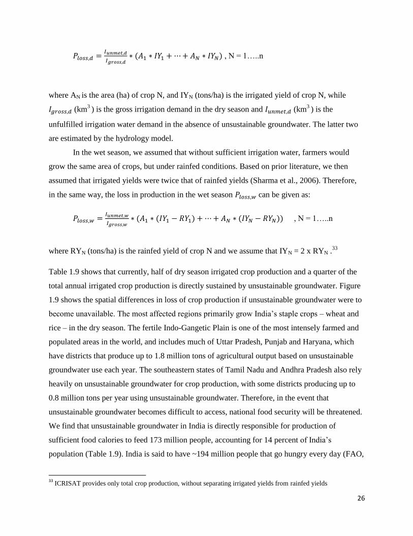
26
𝑃𝑙𝑜𝑠𝑠,𝑑 =𝐼𝑢𝑛𝑚𝑒𝑡,𝑑
𝐼𝑔𝑟𝑜𝑠𝑠,𝑑∗ (𝐴1 ∗ 𝐼𝑌1 + ⋯ + 𝐴𝑁 ∗ 𝐼𝑌𝑁) , N = 1…..n
where AN is the area (ha) of crop N, and IYN (tons/ha) is the irrigated yield of crop N, while
𝐼𝑔𝑟𝑜𝑠𝑠,𝑑 (km3
) is the gross irrigation demand in the dry season and 𝐼𝑢𝑛𝑚𝑒𝑡,𝑑 (km3
) is the
unfulfilled irrigation water demand in the absence of unsustainable groundwater. The latter two
are estimated by the hydrology model.
In the wet season, we assumed that without sufficient irrigation water, farmers would
grow the same area of crops, but under rainfed conditions. Based on prior literature, we then
assumed that irrigated yields were twice that of rainfed yields (Sharma et al., 2006). Therefore,
in the same way, the loss in production in the wet season 𝑃𝑙𝑜𝑠𝑠,𝑤 can be given as:
𝑃𝑙𝑜𝑠𝑠,𝑤 =𝐼𝑢𝑛𝑚𝑒𝑡,𝑤
𝐼𝑔𝑟𝑜𝑠𝑠,𝑤∗ (𝐴1 ∗ (𝐼𝑌1 − 𝑅𝑌1) + ⋯ + 𝐴𝑁 ∗ (𝐼𝑌𝑁 − 𝑅𝑌𝑁)) , N = 1…..n
where RYN (tons/ha) is the rainfed yield of crop N and we assume that IYN = 2 x RYN .33
Table 1.9 shows that currently, half of dry season irrigated crop production and a quarter of the
total annual irrigated crop production is directly sustained by unsustainable groundwater. Figure
1.9 shows the spatial differences in loss of crop production if unsustainable groundwater were to
become unavailable. The most affected regions primarily grow India’s staple crops – wheat and
rice – in the dry season. The fertile Indo-Gangetic Plain is one of the most intensely farmed and
populated areas in the world, and includes much of Uttar Pradesh, Punjab and Haryana, which
have districts that produce up to 1.8 million tons of agricultural output based on unsustainable
groundwater use each year. The southeastern states of Tamil Nadu and Andhra Pradesh also rely
heavily on unsustainable groundwater for crop production, with some districts producing up to
0.8 million tons per year using unsustainable groundwater. Therefore, in the event that
unsustainable groundwater becomes difficult to access, national food security will be threatened.
We find that unsustainable groundwater in India is directly responsible for production of
sufficient food calories to feed 173 million people, accounting for 14 percent of India’s
population (Table 1.9). India is said to have ~194 million people that go hungry every day (FAO,
33
ICRISAT provides only total crop production, without separating irrigated yields from rainfed yields

27
2015); thus losing access to unsustainable groundwater would further aggravate food security
concerns that already plague India. Since our estimates of production losses due to limited access
to unsustainable groundwater are estimated using several first-order assumptions, this analysis
could be extended to study the crop-specific response of farmers to insufficient irrigation water
supplies, as it is likely that subsistence-level food security concerns may drive decisions about
which irrigated crop areas to reduce.34
1.7.2 National River Linking Project and Inter-Basin Transfers
A recent government initiative has looked to the massive National River Linking Project
(NRLP) to overhaul water management in India.35
The $123 billion project intends to move 178
km3 yr
-1 of water by connecting 37 rivers, building ~3000 storage dams and 12,500 km of water
conveyance networks (Chellaney, 2011; Amarsinghe et al., 2009). If completed, it will be the
biggest infrastructure project in the world dwarfing China’s Three Gorges Dam and the South-
North Water Transfer Scheme (Amarsinghe et al., 2009). In addition to its stated goals of 34 GW
of hydropower generation, increasing drinking water supplies, and mitigating floods in the east
(Amarsinghe et al., 2009), it is also expected to alleviate the stress on groundwater. The NRLP is
expected to increase the extent of irrigated agriculture by 35 million ha through surface irrigation
and improved groundwater recharge (Amarsinghe et al., 2009). However, the massive project
faces not only engineering challenges36
but legal, political and societal hurdles as well. Water is
a state subject and inter- state water sharing conflicts, like the Cauvery river water dispute, are
common in India. Geopolitically, countries such as Nepal and Bangladesh will also have to agree
to transfers from rivers shared across boundaries. Moreover, the project is likely to cause
displacement of people who will need to be rehabilitated and resettled. Given these challenges, it
is essential to evaluate the mediating influence of the river linking project on groundwater stress
in India.
To quantify the NRLP’s impact on unsustainable groundwater demand and surface water
irrigation, we simulate a scenario in the hydrology model, in which all proposed river links are
34
Additionally, this analysis can be extended to incorporate endogenous land use decisions. We currently assume
land use decisions have already been made, and therefore do not endogenize decisions to either plant a drought
resistant crop or irrigate more in the face of negative precipitation shocks. 35
The first link between the Krishna and Godavari rivers was launched on September 16, 2015 36
The Krishna-Godavari link saw a massive breech in the aqueduct three days after its launch.

28
functional along with concurrent construction of large reservoirs at receiving nodes in the NRLP,
and compare the unsustainable groundwater demand to our baseline model results.
In our analysis, the hydrology model accounts for all published proposed irrigation water
transfers (both the Himalayan and Peninsular components) across river basins. In addition, it
accounts for existing transfers for which canals have already been completed: the Kurnool
Cuddapah Canal System, the Periyar Project, the Parambikulam Aliyar Project, the Teluga
Ganga Project, and the Indira Gandhi Canal (Ghassemi and White, 2007; Jain et al. , 2005). The
completed transfers were implemented in the year that construction was completed. Proposed
NRLP transfers were turned on for the entire future simulation (2006 – 2050), as there is no set
date for completing construction of these transfers. The impact of the NRLP on unsustainable
groundwater demand was only assessed for the last decade of the simulation, 2040-2050, and so
these results are not sensitive to any construction date prior to 2040.
Two scenarios are simulated: one implements only the inter-basin water transfers through
the proposed canal system; the other additionally adds reservoirs at each water recipient location.
In both simulations, the daily volume of water moved through the canals is a function of river
discharge at the donor location and the canal’s capacity. In the second simulation, reservoir
capacity is added to allow water transferred during the wet season to be stored until it is needed
for irrigation in the dry season37
.
While NRLP plans have included increased water storage (Amarshinghe et al., 2009),
there is insufficient detail on storage methods, locations, or capacities to accurately simulate an
NRLP-storage scenario. We chose to develop a scenario that would allow all wet season water
transfers to be stored until the dry season, then be released to optimize supply during periods of
high irrigation water demand. This scenario is hypothetical, and should only be interpreted as an
upper bound on the potential of the NRLP to alleviate UGW demand. We recognize that there
are other, non-irrigation NRLP goals – particularly hydropower generation (Amarshinghe et al.,
2009) – which may require a different water transfer and storage schedule than modeled here.
Wet season water transfers were stored by implementing large reservoirs at the donor river
37
Water is transferred on a daily time step. Several of the lengthy inter-basin transfers were split into multiple
transfer segments for the purpose of the simulation. This allowed for water to be released and/or stored along the
canal route, from where it can be accessible for irrigation withdrawals.

29
location for each transfer. Each reservoir has a capacity equal to the 10-year average (1996-2005)
simulated wet season transfer volume, and releases water in proportion to the historical irrigation
water demand in the region surrounding the reservoir. Reservoir capacity was limited to the
capacity of the largest existing irrigation reservoir in India (11 km3, Nagarjuna Reservoir;
GRanD database, Lehner et al., 2011). Notably, while the hypothetical NRLP reservoirs in the
northwestern states of Punjab, Haryana, and Gujarat are each < 5km3 in capacity, they sum to a
total of ~15 km3 of increased reservoir capacity through the region. Simulated historical (1990-
2005) UGW demand across these states was ~ 20 km3/year.
We find that with both the additional reservoirs and the inter-basin transfer network
functioning, there is potential to alleviate as much as 16% of India’s mid-century UGW demand
(Fig. 1.10b). However, without new large reservoirs, the inter-basin transfers alone reduce only
1-4% of overall UGW demand (Fig. 1.10c). This small percentage is primarily due to the
transfer rules; since a percentage of donor-river discharge is transferred, the largest water
transfers occur in the wet (Kharif) season, while the majority of UGW demand occurs in the dry
(Rabi) season.
Historically, construction of large dams has been contentious in India (Dhawan, 1989;
Fisher, 1995). While the exact plans for dam construction under the NRLP have not yet been
publicized, it is clear from these results that without a large increase in reservoir capacity, the
NRLP will not alleviate groundwater stress in northwest India. While we provide a preliminary
analysis of the effects of the NRLP on groundwater stress, a detailed economic analysis about the
efficiency of water allocation by the NRLP is an important area of future work. Estimating the
steepness of the water demand function for users across basins can help asses if the NRLP is
allocating water to its highest use, and therefore efficiently allocating water.
1.8 Conclusion
Over the past forty years, the use of groundwater has shaped the course of agrarian
change and development in India. It is important to assess whether the impact of a changing
climate will accentuate or reduce groundwater use, since groundwater access is salient to the
livelihoods of millions of small and marginal farmers, and parts of India are already experiencing
groundwater depletion. In this paper, we provide the first multi-model assessment of the extent
of unsustainable groundwater use in India by mid-century, its importance in sustaining food

30
production, and the role that government adaptation through investments in large infrastructure
projects might play in decreasing India’s dependence on unsustainable groundwater in the future.
Our econometric results show that inter-annual variation in the monsoon plays a
fundamental role in agricultural decision-making in India. Here, we investigate its role on
irrigation decisions across seasons and major crops. We find that while irrigation expands, on
average, in response to an uneven distribution of rain in the wet season; crops like Rabi rice and
wheat grown in the dry season are largely dependent on monsoon rainfall for their irrigation
needs, so that a fall in precipitation also leads to a reduction in irrigation. As the monsoon
changes with climate change, changes in groundwater use and availability will also be seen. By
coupling both the econometric and hydrology models we are able to identify regions where
groundwater demand and supply may change significantly in the future (Figures 1.7 and 1.9 ),
and such insight has important implications for policy decisions that affect agricultural
development, poverty, food security, and adaptation.
One policy recommendation for managing water is the NRLP, but our results
demonstrate canals alone have limited ability to decrease unsustainable use of groundwater
nationally, if current irrigation practices continue. While increasing the country’s reservoir
capacity along the NRLP canals may significantly increase the project’s potential to alleviate
groundwater stress, construction of large reservoirs such as those simulated here is likely to be
controversial. In addition to the NRLP project, several other tools have shown some promise in
reducing groundwater extraction in different areas. These include investments in public provision
of groundwater to crowd out private construction of wells (Sekhri, 2011), decentralized rainwater
harvesting schemes (Sekhri, 2012), creation of groundwater markets (Foster and Sekhri, 2008),
and rationing of power supply by separating agricultural from non-agricultural feeders (Shah and
Verma, 2008). It is possible, or even likely, that multiple strategies will be employed over time;
therefore, further assessment of the NRLP in conjunction with other infrastructure and policy
measures should be conducted to identify potential synergies and conflicts.

31
References
Abler, D., G. S. Tollow, and G. K. Kripalani (1994) Technical Change & Income Distribution in
Indian Agriculture, Westview Press, 1994
Aeschbach-Hertig, W. and T. Gleeson (2012) Regional strategies for the accelerating global
problem of groundwater depletion, Nat Geosci, 5(12), 853-861.
Amarasinghe, U. A., K. Palanisami, O. Singh, and R. Sakthivadivel (2009) State of Irrigation in
Tamil Nadu: Investments and Returns, Strategic Analyses of the National River Linking Project
(NRLP) of India Series, IWM1
Amarasinghe U.A., T. Shah and R.P.S. Malik (2009) Strategic Analyses of the National River
Linking Project (NRLP) of India Series 1, India’s Water Future: Scenarios and Issues, IWMI.
Ashfaq, M.,Y. Shi, W.Tung, R. J. Trapp, X. Gao, J. S. Pal, and N. S. Diffenbaugh (2009)
Suppression of south Asian summer monsoon precipitation in the 21st century. Geophys Res Lett
36, L01704, doi:10.1029/2008GL036500.
Auffhammer M., V. Ramanathan and J. Vincent J (2012) Climate change, the monsoon, and rice
yield in India. Clim Change 111(2):411-424.
Auffhammer M., S.M. Hsiang, W. Schlenker and A. Sobel (2013) Using weather data and
climate model output in economic analyses of climate change. Review of Environmental
Economics and Policy 7 (2): 181-198.
Auffhammer, M. and W. Schlenker (2014) Empirical studies on agricultural impacts and
adaptation, Energy Economics 46: 555-561
Badiani R., K.K. Jessoe and S. Plant (2012) Development and the environment: the implications
of agricultural electricity subsidies in India, The Journal of Environment & Development 21(2):
244-262
Banzhaf H.S. and N. Lavery (2010) Can the land tax help curb urban sprawl? Evidence from
growth patterns in Pennsylvania. Journal of Urban Economics 67(2):169-179
Bhat, G.S. (2006) The Indian drought of 2002-a sub-seasonal phenomenon? Q J R Meteorol Soc
132(621): 2583-2602.
Brouwer C. and M. Heibloem (1986) Irrigation Water Management Training Manual No. 3:
Irrigation Water Needs, Food and Agriculture Organization of the United Nations.
Bruinsma, J. et al. (2009) The resource outlook to 2050: by how much do land, water and crop
yields need to increase by 2050? in How to feed the World in 2050. Proceedings of a technical
meeting of experts, Rome, Italy, 24-26 June 2009, Food and Agriculture Organization of the
United Nations (FAO), 1-33.

32
Burke, M. and K. Emerick (2015) Adaptation to climate change: Evidence from US agriculture.
Am Econ J Econ Policy (in press).
Chamberlain, G. (1984) Handbook of Econometrics, vol. 2. Panel Data, eds Griliches Z,
Intriligator MD (North-Holland, Amsterdam), pp. 1247–1318
Chaturvedi, R.K., J. Joshi, M. Jayaraman, G. Bala and N. Ravindranath (2012) Multi-model
climate change projections for India under representative concentration pathways. Curr Sci
103(7): 791-802
Chellaney, B. (2011) Water: Asia’s New Battleground (Georgetown University Press,
Washington DC), pp 210-215.
Dell, M., B. Jones and B. Olken (2014) What Do We Learn from the Weather? The New
Climate-Economy Literature. J Econ Lit 52(3): 740-798
Deschenes, O. and M. Greenstone. (2007) The Economic Impacts of Climate Change: Evidence
from Agricultural Output and Random Fluctuations in Weather, American Economic Review,
97(1): 354-385.
Dhawan, B.D. (1989) Mounting antagonism towards big dams. Economic and Political Weekly
24(20): 1096-1099.
Duflo, E. and R. Pande (2007) Dams, Quarterly Journal of Economics, 122(2):601-646
Elliott, J., et al. (2014) Constraints and potentials of future irrigation water availability on
agricultural production under climate change, Proceedings of the National Academy of Sciences,
111(9), 3239-3244.
Famiglietti, J.S., et al. (2011) Satellites measure recent rates of groundwater depletion in
California’s Central Valley, Geophys Res Lett 38, L03403, doi:10.1029/2010GL046442.
Fisher, W.F. (1995) Toward sustainable development: Struggling over India's Narmada River.
Development and Resistance in the Narmada Valley, ed Fisher WF(ME Sharpe, New York), pp
3-45
Fishman, R. M., T. Siegfried, P. Raj, V. Modi, and U. Lall (2011) Over-extraction from shallow
bedrock versus deep alluvial aquifers: Reliability versus sustainability considerations for India's
groundwater irrigation, Water Resources Research, 47(6) W00L05
Fishman, R. M. (2012) Climate change, rainfall variability, and adaptation through irrigation:
Evidence from Indian agriculture, Working Paper
Fishman, R. U. Lall, V. Modi and N. Parekh (2014) Can Electricity Pricing Save India's
Groundwater? Evidence from Gujarat, Working Paper
33
Ferguson, G. and T. Gleeson (2012) Vulnerability of coastal aquifers to groundwater use and
climate change, Nature Climate Change 2(5):342-345.
Fischer, G., F. N. Tubiello, H. Van Velthuizen, and D. A. Wiberg (2007) Climate change
impacts on irrigation water requirements: effects of mitigation, 1990-2080, Technological
Forecasting and Social Change, 74, 1083-1107.
Food and Agriculture Organization of the United Nations (FAO) (2015) The State of Food
Insecurity in the World 2015.
Foster, A. D. and M. R. Rosenzweig (1996) Technical change and human-capital returns and
investments: evidence from the Green Revolution, American Economic Review, 931-953.
Foster A. and S. Sekhri (2008) Can expansion of markets for groundwater decelerate the
depletion of groundwater resources in rural India. Working Paper
Frolking, S., J.B. Yeluripati and E. Douglas (2006) New district-level maps of rice cropping in
India: a foundation for scientific input into policy assessment. Field Crops Res 98(2-3): 164-177.
Gadgil, S and K.R. Kumar (2006) The Asian Monsoon- agriculture and economy. The Asian
Monsoon, ed Wang B (Springer/Praxis Publishing, Honolulu), pp 660-670
Gandhi, V.P. and N.V. Namboodiri (2009) Groundwater irrigation in India: Gains, costs, and
risks. Ahmedabad, India: Indian Institute of Management.
Ghassemi, F. and I. White (2007) Inter-Basin Water Transfer: Case Studies from Australia,
United States, Canada, China and India (Cambridge: Cambridge University Press)
Giné, X. and H. Jacoby (2015) Markets, Contracts, and Uncertainty: A Structural Model of a
Groundwater Economy, Working Paper
Government of India (2012) State of Indian Agriculture 2012-13, Report, Department of
Agriculture and Co-operation, New Delhi.
Greene, W. H. (2003) Econometric analysis, 5th. Ed. Upper Saddle River, NJ.
Greene, W. H. (2004) Fixed effects and bias due to the incidental parameters problem in the
Tobit model. Econometric Reviews 23(2):125-147
Grogan, D.S., F. Zhang, A. Prusevich, R.B. Lammers, D. Wisser, S. Glidden, C. Li and S.
Frolking (2015) Quantifying the link between crop production and mined groundwater irrigation
in China. Sci Total Environ 511: 161-175, doi:10.1016/j.scitotenv.2014.11.076
Guiteras, R. (2009) The impact of climate change on Indian agriculture, Manuscript, Department
of Economics, University of Maryland, College Park, Maryland

34
Hanasaki, N et al. (2013) A global water scarcity assessment under shared socio-economic
pathways{Part 1: Water use," Hydrology and Earth System Sciences, 17, 2375-2391.
Honoré, B., F. Vella and M.Verbeek (2008) Attrition, selection bias and censored regressions.
The Econometrics of Panel Data, eds Mátyás L, Sevestre P (Springer, Berlin Heidelberg ), pp.
385-418
Hsiang, S.M. (2010) Temperatures and cyclones strongly associated with economic production
in the Caribbean and Central America. Proceedings of the National Academy of Sciences USA
107(35): 15367-15372.
Hu Z., M. Latif, E. Roeckner and L. Bengtsson (2000) Intensified Asian summer monsoon and
its variability in a coupled model forced by increasing greenhouse gas concentrations, Geophys
Res Lett 27(17): 2681-2684.
Huke, R.E. and E.H. Huke (1997) Rice Area by Type of Culture: South, Southeast, and East Asia:
A Revised and Updated Data Base. International Rice Research Institute (IRRI, Los Baños)
Jack, B.K. (2011) Constraints on the adoption of agricultural technologies in developing
countries. White paper, Agricultural Technology Adoption Initiative, J-PAL (MIT) and CEGA
(UC Berkeley).
Jain, S. K., N. S. R. K. Reddy, and U.C. Chauge (2005) Analysis of a large inter-basin water
transfer system in India, Hydrolog. Sci. J. 50 1-137
Jain, S., P. Agarwal, and V. Singh (2007) Hydrology and Water Resources of India, Water
Science and Technology Library, Springer
Kazmin, A. (2012) India’s farmers pray for rain, Financial Times, July 25, 2012
Kharol, S. K., D. Kaskaoutis, A. R. Sharma, and R. P. Singh (2013) Long-Term (1951-2007)
Rainfall Trends around Six Indian Cities: Current State, Meteorological, and Urban Dynamics,
Advances in Meteorology, http://dx.doi.org/10.1155/2013/572954
Konzmann, M., D. Gerten and J. Heinke (2013) Climate impacts on global irrigation
requirements under 19 GCMs, simulated with a vegetation and hydrology model, Hydrology
Science Journal, 58(1):88–105
Kumar, K. and J. Parikh (2001) Indian agriculture and climate sensitivity, Global Environmental
Change, 1:147–154
Kurukulasuriya, P., N. Kala, and R. Mendelsohn (2011) Adaptation and Climate Change Impacts:
A Structural Ricardian Model Of Irrigation And Farm Income in Africa, Climate Change
Economics, 2(02):149–174
35
Lal, M., et al. (2001) Future climate change: Implications for Indian summer monsoon and its
variability, Curr Sci 81(9): 1196-1207
Lancaster, T. (2000) The incidental parameters problem since 1948, Journal of Econometrics
95(2), 391-413.
Lehner, B. et al. (2011) High-resolution mapping of the world's reservoirs and dams for
sustainable river-flow management, Front. Ecol. Environ 9, 494-502
Leng, G. and Q. Tang (2014) Modeling the impacts of future climate change on irrigation
over China: sensitivity to adjusted projections, Journal of Hydrometeorology, 15, 2085-2103.
Majumdar, D.K. (2013) Irrigation Water Management: Principles and Practice, Second Edition
(PHI Learning Pvt. Ltd., Delhi), pp 295-399
Meehl, G. and J. Arblaster (2003) Mechanisms for projected future changes in south Asian
monsoon precipitation, Climate Dynamics, 21, 659-675
Mehta, V. K., V. R. Haden, B. A. Joyce, D. R. Purkey, and L. E. Jackson (2013) Irrigation
demand and supply, given projections of climate and land-use change, in Yolo County,
California, Agricultural Water Management, 70 -82 doi: 10.1016/j.agwat.2012.10.021.
Mendelsohn, R., W. D. Nordhaus, and D. Shaw (1994) The impact of global warming on
agriculture: a Ricardian analysis, American Economic Review, 84(4): 753-771.
Mendelsohn, R., A. Dinar, and L. Williams (2006) The distributional impact of climate change
on rich and poor countries, Environment and Development Economics, 11(02):159-178
Menon, A., A. Levermann, J. Schewe, J. Lehmann and K. Frieler (2013) Consistent increase in
Indian monsoon rainfall and its variability across CMIP-5 models. Earth Sys Dynam 4(2): 287-
300
Miller, B. M. (2015) Does Validity Fall from the Sky? Observant Farmers, Exogenous Rainfall,
and Climate Change, Manuscript, UCSD.
Ministry of Agriculture (2014) Agricultural Statistics at a Glance 2014, Directorate of
Economics and Statistics, Government of India.
Mukherji, A., S. Rawat, and T. Shah (2013) Major Insights from India’s Minor Irrigation
Censuses: 1986-87 to 2006-07, Economic & Political Weekly, 48, 28.
Neyman, J. and E. Scott (1948) Consistent Estimates Based on Partially Consistent Observations.
Econometrica 16(1):1-32
Nickell, S. (1981) Biases in dynamic models with fixed effects. Econometrica 49(6):1417-1426.

36
NSSO (National Sample Survey Office) (2014) Key Indicators of Situation of Agricultural
Households in India. Ministry of Statistics and Programme Implementation, Government of
India.
Rajeevan, M. and J. Bhate (2009) A high resolution daily gridded rainfall dataset (1971-2005)
for mesoscale meteorological studies, Curr. Sci, 96, 558-562
Rodell, M., I. Velicogna and J.S. Famiglietti (2009) Satellite-based estimates of groundwater
depletion in India. Nature, 460(7258), 999-1002.
Roodman, D. (2009) How to do xtabond2: An introduction to difference and system GMM in
Stata, Stata Journal, 9, 86.
Rosenzweig, M. R. and H. P. Binswanger (1993) Wealth, Weather Risk and the Composition
and Profitability of Agricultural Investments, Economic Journal, 103, 56-78.
Rosenzweig, M. and C. R. Udry (2013) Forecasting profitability, NBER Working Paper
Rud, J. P. (2012) Electricity provision and industrial development: Evidence from India, Journal
of development Economics, 97(2): 352-367
Sanghi, A., R. Mendelsohn, and A. Dinar (1998) The climate sensitivity of Indian agriculture,
Chapter 4 in Measuring the impact of climate change on Indian agriculture, World Bank
Technical Paper 402.
Schlenker, W., W. M. Hanemann, and A. C. Fisher (2005) Will US agriculture really
benefit from global warming? Accounting for irrigation in the hedonic approach, American
Economic Review, 395-406.
Schlenker, W., W. M. Hanemann, and A. C. Fisher (2006) The impact of global warming on US
agriculture: an econometric analysis of optimal growing conditions, Review of Economics and
Statistics, 88, 113-125.
Schlenker, W. and M. J. Roberts (2009) Nonlinear temperature e_ects indicate severe damages
to US crop yields under climate change, Proceedings of the National Academy of Sciences,
106, 15594-15598.
Sekhri, S. (2011) Public provision and protection of natural resources: Groundwater irrigation
in rural India, American Economic Journal: Applied Economics, 3(4): 29-55.
Sekhri, S. (2012) Sustaining Groundwater: Role of Policy Reforms in Promoting Conservation in
India. India Policy Forum Volume 9, eds Shah S, Bosworth B, Panagariya A (Sage Publications,
New Delhi), pp 149-186.
Sekhri, S. (2013) Missing Water: Agricultural Stress and Adaptation Strategies in Response to
Groundwater Depletion in India, Working Paper

37
Sekhri, S. (2014) Wells, Water, and Welfare: The Impact of Access to Groundwater on Rural
Poverty and Conflict. Am Econ J Appl Econ 6(3), 76-102.
Shah T. and S. Verma (2008) Co-management of electricity and groundwater: an assessment of
Gujarat’s Jyotirgram Scheme. Economic and Political Weekly, 43(7): 59-66
Shah, T. and A. Kishore (2009) Will the Impact of the 2009 Drought Be Different from 2002?"
Economic and Political Weekly, 11-14.
Shah, T. (2010) Taming the Anarchy: Groundwater Governance in South Asia, Resources for the
Future Press, Washington DC.
Shah, M. (2013) Water: Towards a paradigm shift in the twelfth plan, Economic & Political
Weekly, 48, 41.
Shah, T. (2011) Past, present, and the future of canal irrigation in India," India Infrastructure
Report, IDFC.
Sharma, B. R., B. Sharma, K. V. Rao, K. P. R. Vittal and A. U. Amarasinghe (2006) Realizing
the potential of rainfed agriculture in India. (Drafts prepared for the IWMI-CPWF project on
‘Strategic Analysis of India’s National River-Linking Project’ IWMI
Siebert, S. and P. Doll (2010) Quantifying blue and green virtual water contents in global crop
production as well as potential production losses without irrigation, Journal of Hydrology 384(3-
4): 198-217.
Siegfried, T., S. Sobolowski, P. Raj, R. Fishman, V. Vasquez, K. Narula, U. Lall, and V. Modi
(2010) Modeling irrigated area to increase water, energy, and food security in semiarid India,
Weather, Climate, and Society, 2, 255-270.
Singh, RB, Kumar P, Woodhead T (2002) Smallholder farmers in India: Food Security and
Agricultural Policy. FAO Regional Office for Asia and the Pacific, Bangkok, Thailand.
Singh, D., M. Tsiang, B. Rajaratnam, and N. S. Diffenbaugh (2014) Observed changes in
extreme wet and dry spells during the South Asian summer monsoon season, Nature Climate
Change 4(6), 456-461.
Sooraj, K.P., P. Terray and M. Mujumdar (2014), Global warming and the weakening of the
Asian summer monsoon circulation: assessments from the CMIP5 models. Clim Dyn 45(1-2):
233-252
Sue Wing, I. and E. De Cian (2014) Integrated assessment: Modelling agricultural adaptation.
Nat Clim Chang, 4(7): 535-536.
Taraz, V. (2015) Adaptation to Climate Change: Historical Evidence from the Indian Monsoon,
38
Yale University Working Paper
Taylor, R. G., B. Scanlon, P. Doll, M. Rodell, R. Van Beek, Y. Wada, L. Longuevergne,
M.Leblanc, J.S. Famiglietti, M. Edmunds, et al. (2013) Ground water and climate change, Nature
Climate Change 3(4): 322-329
UNFCCC (2007). Investment and financial vows to address climate change. Bonn: UNFCCC
Ummenhofer, C. C., A. S. Gupta, Y. Li, A. S. Taschetto, and M. H. England (2011) Multi-
decadal modulation of the El Nino–Indian monsoon relationship by Indian Ocean variability,
Environmental Research Letters 6(3) 034006.
Vaidyanathan, A. (2010) Agricultural Growth in India: The Role of Technology, Incentives, and
Institutions, Oxford University Press India
Wada, Y., D. Wisser, S. Eisner, M. Florke, D. Gerten, I. Haddeland, N. Hanasaki, Y. Masaki, F.
T. Portmann, T. Stacke, et al. (2013) Multimodel projections and uncertainties of irrigation water
demand under climate change, Geophysical Research Letters, 40, 4626-4632
Wang, B. (2006) The Asian Monsoon, Springer Praxis Books / Environmental Sciences, Springer.
Wooldridge, J.M. (2010) Econometric analysis of cross section and panel data (MIT press,
Cambridge, MA)
World Bank (1998) India - Water resources management sector review: groundwater regulation
and management report. World Development Sources, World Bank
World Bank (2014) Global Monitoring Report 2014/2015: Ending Poverty and Sharing
Prosperity, World Bank, Washington DC, doi: 10.1596/978-1-4648-0336-9.
Yasutomi, N., A. Hamada and A. Yatagai (2011) Development of a long-term daily gridded
temperature dataset and its application to rain/snow discrimination of daily precipitation, Global
Environmental Research 15(2):165-172.
Yatagai A., et al. (2012) APHRODITE: Constructing a Long-term Daily Gridded Precipitation
Dataset for Asia based on a Dense Network of Rain Gauges, Bulletin of American
Meteorological Society, 93, 1401-1415, doi:10.1175/BAMS-D-11-00122.1.
Yatagai A., et al. (2009) A 44-year daily gridded precipitation dataset for Asia based on a dense
network of rain gauges, SOLA, 5, 137-140, doi:10.2151/sola.2009-035

39
Human System Identifying
sensitivity of
irrigated area to
weather changes
Climate
Inputs
Physical System Hydrology model to
represent spatial
and temporal water
cycle
Future Crop
irrigated area by
season
Water Model
Input
Δ Irrigation Water
Demand
Δ Unsustainable
Water Demand
Results Econ Model
Output
Figures
Fig. 1.1: Aggregate Changes in Wheat and Rice Area, Irrigation and Production
Notes: Each panel reports values aggregated in each period over the district sample used in the analysis of (A) rice
and(B) wheat, with values of log irrigated area, log crop area and log production reported on the right axis. Blue bars
are normalized monsoon anomalies (MA), whose values are reported on the left axis. Crop data are from ICRISAT,
and monsoon anomalies are from the APHRO_MA_V1101R2 precipitation product.
Fig. 1.2. Coupled Human and Physical System Model Schematic
Notes: Human system analysis uses an econometric model to identify historical irrigated area sensitivity to weather
changes. Climate drivers from 5 GCMs are combined with historical regression estimates to project future crop-wise
irrigated areas. These projections, and the climate drivers, are inputs to a physically-based hydrology model, which
simulates future irrigation water demand and unsustainable groundwater demand.
A B

40
Fig. 1.3a: Average Historical Monsoon Rainfall and No. of Rainy Days (June-September)
Notes: Average (1970-2005) (A) June to September monsoon rainfall (mm), and (B) number of monsoon rainy days
(days with precipitation>0.1mm from June to September). Gridded APHRO_MA_V1101R2 data were aggregated to
district values; state borders are in black.
Fig. 1.3b: Historical Inter-annual and Inter-decadal Variability in Monsoon Rainfall (June-
September)
Notes: Source: Wang (2006). Inter-annual (bar) and Inter-decadal (solid) Variability in All India Rainfall (AIR)
during June-September (JJAS) from 1871 to 2004.
A B
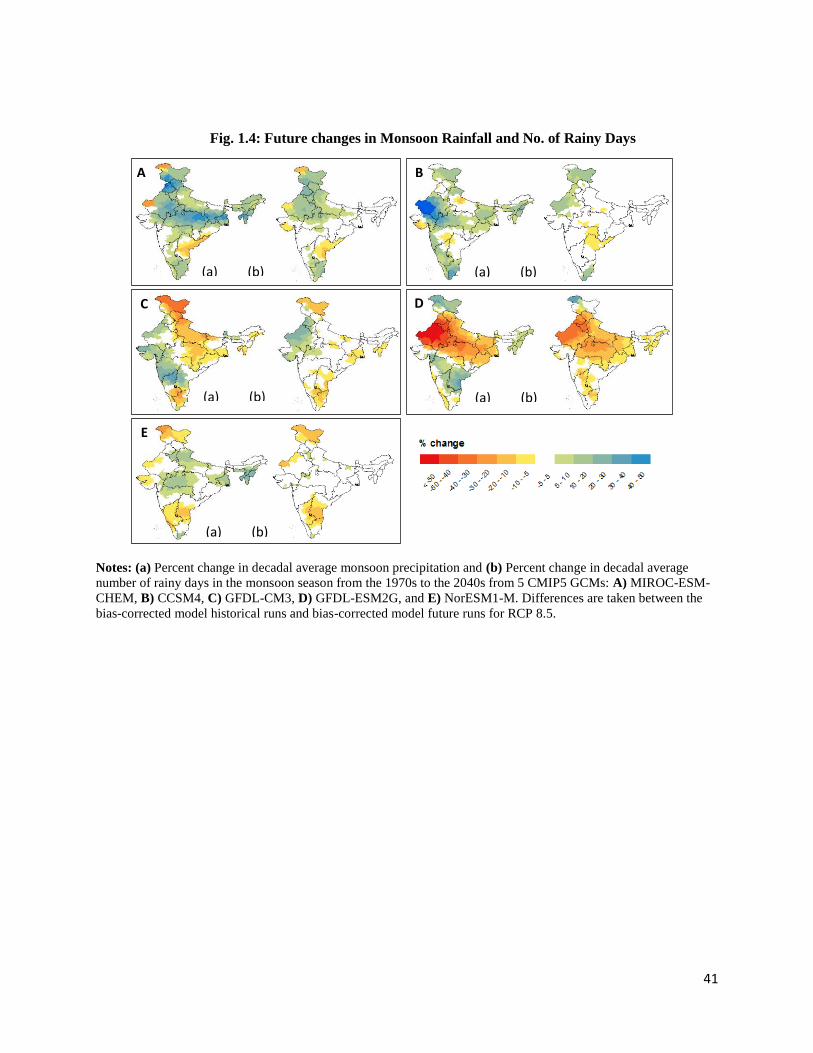
41
Fig. 1.4: Future changes in Monsoon Rainfall and No. of Rainy Days
Notes: (a) Percent change in decadal average monsoon precipitation and (b) Percent change in decadal average
number of rainy days in the monsoon season from the 1970s to the 2040s from 5 CMIP5 GCMs: A) MIROC-ESM-
CHEM, B) CCSM4, C) GFDL-CM3, D) GFDL-ESM2G, and E) NorESM1-M. Differences are taken between the
bias-corrected model historical runs and bias-corrected model future runs for RCP 8.5.
A B
C D
E
(a) (b) (a) (b)
(a) (b) (a) (b)
(a) (b)
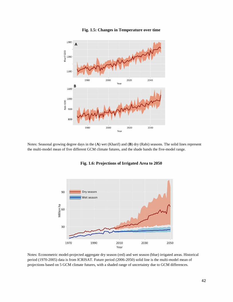
42
Fig. 1.5: Changes in Temperature over time
Notes: Seasonal growing degree days in the (A) wet (Kharif) and (B) dry (Rabi) seasons. The solid lines represent
the multi-model mean of five different GCM climate futures, and the shade bands the five-model range.
Fig. 1.6: Projections of Irrigated Area to 2050
Notes: Econometric model-projected aggregate dry season (red) and wet season (blue) irrigated areas. Historical
period (1970-2005) data is from ICRISAT. Future period (2006-2050) solid line is the multi-model mean of
projections based on 5 GCM climate futures, with a shaded range of uncertainty due to GCM differences.
A
B

43
Fig. 1.7: Trends in Groundwater Levels between 1979-2000 and 2029-2050
Notes: Trends in district-level ground water levels (GWL) between 1979-2000 and 2029-2050, inferred from the
multi-model mean of changing need for unsustainable groundwater (UGW) to meet irrigation water needs.
Decreases in UGW demand will slow down GWL declines (yellow); continued demand will lead to continued GWL
declines (red); increased demand will increase GWL declines (dark red); new positive demands can start GWL
declines (orange); demand going to 0 can allow GWL to recover (blue). Black lines are state boundaries . Colored
(non-grey) regions account for 90% of future modeled national UGW demand. Appendix Fig. 3 shows trends in
GWL for 5 individual GCM climate futures.

44
Fig. 1.8: Volume of Unmet Irrigation Water Demand in Absence of Unsustainable
Groundwater
Notes: Annual unmet irrigation water demand (km
3) if unsustainable groundwater supplies were unavailable
historically (1970-2005) and in the future (2006-2050). Future multi-model mean (solid line) and range (shaded) are
based on 5 GCM climate futures, with uncertainty due to differences in GCM projections.
Fig. 1.9: Crop Production (million tons) Dependent on Unsustainable Groundwater
Notes: District-level reduction in current (c. year 2000) annual crop production, in million metric tons, that
would occur if unsustainable groundwater supplies became unavailable. Black lines are state boundaries.
A B
C
E F
D
G

45
Fig 1.10: National River Linking Project and Unsustainable Groundwater
Notes: A) Mid-century annual unsustainable groundwater (UGW) demand at the district level. The National River
Linking Project (NRLP) is a proposed solution for alleviating this demand. B) and C) Light blue lines: NRLP water
transfer canals; red dots: water donor locations; blue dots: water recipient locations. Blue dots along chained canals
are both receiving and donating. B) The % of each district’s mid-century UGW demand that could be alleviated with
the implementation of NRLP canals and construction of new reservoirs along canal routes. Blue: UGW demand is
alleviated; yellow and red: UGW demand is worsened. National total UGW alleviation is 16%. C) The % of each
district’s mid-century UGW demand that could be alleviated with the implementation of NRLP canals only.
National UGW alleviation is 1-4% with transfers only. Gray lines are state boundaries. B) and C) share a scale bar.
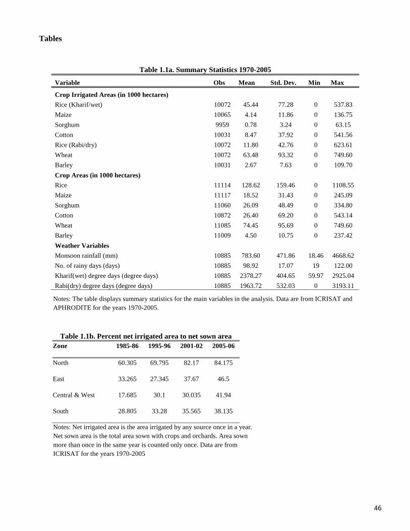
46
Tables
Notes: The table displays summary statistics for the main variables in the analysis. Data are from ICRISAT and
APHRODITE for the years 1970-2005.
Notes: Net irrigated area is the area irrigated by any source once in a year.
Net sown area is the total area sown with crops and orchards. Area sown
more than once in the same year is counted only once. Data are from
ICRISAT for the years 1970-2005
Table 1.1a. Summary Statistics 1970-2005
Variable Obs Mean Std. Dev. Min Max
Crop Irrigated Areas (in 1000 hectares)
Rice (Kharif/wet) 10072 45.44 77.28 0 537.83
Maize 10065 4.14 11.86 0 136.75
Sorghum 9959 0.78 3.24 0 63.15
Cotton 10031 8.47 37.92 0 541.56
Rice (Rabi/dry) 10072 11.80 42.76 0 623.61
Wheat 10072 63.48 93.32 0 749.60
Barley 10031 2.67 7.63 0 109.70
Crop Areas (in 1000 hectares)
Rice 11114 128.62 159.46 0 1108.55
Maize 11117 18.52 31.43 0 245.09
Sorghum 11060 26.09 48.49 0 334.80
Cotton 10872 26.40 69.20 0 543.14
Wheat 11085 74.45 95.69 0 749.60
Barley 11009 4.50 10.75 0 237.42
Weather Variables
Monsoon rainfall (mm) 10885 783.60 471.86 18.46 4668.62
No. of rainy days (days) 10885 98.92 17.07 19 122.00
Kharif(wet) degree days (degree days) 10885 2378.27 404.65 59.97 2925.04
Rabi(dry) degree days (degree days) 10885 1963.72 532.03 0 3193.11
Table 1.1b. Percent net irrigated area to net sown area
Zone 1985-86 1995-96 2001-02 2005-06
North 60.305 69.795 82.17 84.175
East 33.265 27.345 37.67 46.5
Central & West 17.685 30.1 30.035 41.94
South 28.805 33.28 35.565 38.135

47
Notes: Variation of monsoon precipitation and number of rainy days absorbed by fixed effects. Panel A summarizes regressions of
monsoon precipitation and no. of rainy days on various sets of fixed effects. Columns (a) report the R-square of the regression and
Columns (b) report the standard deviation of the residuals (remaining monsoon precipitation, and no. of rainy days variation) in
mm and days. Panel B reports the percentage of observations (Columns (b)) with absolute value of residuals greater than the
projected change in precipitation and number of rainy days between 1970-79 and 2040-29 as shown in Columns (a)
Panel A
Monsoon
precipitation(mm)
Frequency of rainy days
1a 1b 2a 2b
R sq SD of
residual
R sq SD of
residual
No FE 428.9242 18.01787
Year Fe 0.0346 421.4372 0.0998 17.09494
District FE 0.8238 180.0324 0.7336 9.29931
District FE, Year FE 0.8539 161.3846 0.8334 7.353272
District FE, Year FE, state specific trend 0.8553 160.5031 0.8365 7.285278
Panel B
Monsoon
precipitation(mm)
Frequency of rainy days
3a 3b 4a 4b
Projected
change
%
observations
Projected
change
%
observations
NorESM1-M 27.5 83 -1.4 77
MIROC-ESM_CHEM 82.31 54 3.55 56
CCSM4 50.89 70 -0.13 99
GFDL-CM3 -15.69 92 -1.02 88
GFDL-ESM2G -53.87 69 -8.4 25
Table 1.2: Residual variation in weather
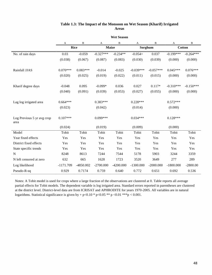
48
Notes: A Tobit model is used for crops where a large fraction of the observations are clustered at 0. Table reports all average
partial effects for Tobit models. The dependent variable is log irrigated area. Standard errors reported in parentheses are clustered
at the district level. District-level data are from ICRISAT and APHRODITE for years 1970-2005. All variables are in natural
logarithms. Statistical significance is given by + p<0.10 * p<0.05 ** p <0.01 ***p < 0.001.
Table 1.3: The Impact of the Monsoon on Wet Season (Kharif) Irrigated
Areas
Wet Season
A B A B A B A B
Rice Maize Sorghum Cotton
No. of rain days 0.03 -0.059 -0.327*** -0.234** -0.054+ 0.037 -0.199*** -0.264***
(0.038) (0.067) (0.087) (0.083) (0.030) (0.039) (0.000) (0.000)
Rainfall JJAS 0.070*** 0.083*** -0.014 -0.025 -0.039*** -0.057*** 0.045*** 0.076***
(0.020) (0.025) (0.019) (0.022) (0.011) (0.015) (0.000) (0.000)
Kharif degree days -0.048 0.095 -0.099* 0.036 0.027 0.117* -0.310*** -0.150***
(0.040) (0.091) (0.039) (0.053) (0.027) (0.055) (0.000) (0.000)
Lag log irrigated area 0.664*** 0.383*** 0.228*** 0.572***
(0.023) (0.042) (0.014) (0.000)
Log Previous 5 yr avg crop
area
0.107*** 0.099*** 0.034*** 0.128***
(0.024) (0.019) (0.009) (0.000)
Model Tobit Tobit Tobit Tobit Tobit Tobit Tobit Tobit
Year fixed effects Yes Yes Yes Yes Yes Yes Yes Yes
District fixed effects Yes Yes Yes Yes Yes Yes Yes Yes
State specific trends Yes Yes Yes Yes Yes Yes Yes Yes
N 8248 8613 7244 7544 5178 5903 3244 3359
N left censored at zero 632 665 1628 1723 3520 3649 277 289
Log likelihood -1171.709 -4850.002 -2700.000 -4200.000 -1300.000 -2000.000 -1800.000 -2800.00
Pseudo-R-sq 0.929 0.7174 0.759 0.640 0.772 0.651 0.692 0.536
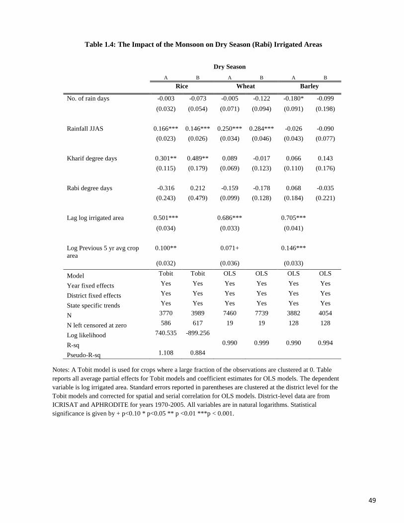
49
Notes: A Tobit model is used for crops where a large fraction of the observations are clustered at 0. Table
reports all average partial effects for Tobit models and coefficient estimates for OLS models. The dependent
variable is log irrigated area. Standard errors reported in parentheses are clustered at the district level for the
Tobit models and corrected for spatial and serial correlation for OLS models. District-level data are from
ICRISAT and APHRODITE for years 1970-2005. All variables are in natural logarithms. Statistical
significance is given by + p<0.10 * p<0.05 ** p <0.01 ***p < 0.001.
Dry Season
A B A B A B
Rice Wheat Barley
No. of rain days -0.003 -0.073 -0.005 -0.122 -0.180* -0.099
(0.032) (0.054) (0.071) (0.094) (0.091) (0.198)
Rainfall JJAS 0.166*** 0.146*** 0.250*** 0.284*** -0.026 -0.090
(0.023) (0.026) (0.034) (0.046) (0.043) (0.077)
Kharif degree days 0.301** 0.489** 0.089 -0.017 0.066 0.143
(0.115) (0.179) (0.069) (0.123) (0.110) (0.176)
Rabi degree days -0.316 0.212 -0.159 -0.178 0.068 -0.035
(0.243) (0.479) (0.099) (0.128) (0.184) (0.221)
Lag log irrigated area 0.501*** 0.686*** 0.705***
(0.034) (0.033) (0.041) Log Previous 5 yr avg crop
area
0.100** 0.071+ 0.146***
(0.032) (0.036) (0.033)
Model Tobit Tobit OLS OLS OLS OLS
Year fixed effects Yes Yes Yes Yes Yes Yes
District fixed effects Yes Yes Yes Yes Yes Yes
State specific trends Yes Yes Yes Yes Yes Yes
N 3770 3989 7460 7739 3882 4054
N left censored at zero 586 617 19 19 128 128
Log likelihood 740.535 -899.256
R-sq 0.990 0.999 0.990 0.994
Pseudo-R-sq 1.108 0.884
Table 1.4: The Impact of the Monsoon on Dry Season (Rabi) Irrigated Areas
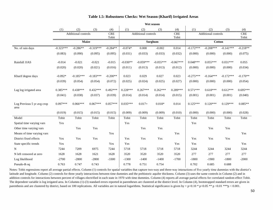
50
Notes: Tobit regressions report all average partial effects. Column (1) controls for spatial variables that capture two-way and three-way interactions of five yearly time dummies with the district’s
latitude and longitude. Column (2) controls for three yearly interactions between time dummies and the prehistoric aquifer thickness. Column (3) uses the same controls in Column (2) and in
addition controls for interactions between percent of villages electrified in each state in 1970 with time dummies. Column (4) reports all average partial effects for correlated random effect Tobit.
The dependent variable is log irrigated area. In Columns (1)-(3) standard errors reported in parentheses are clustered at the district level. In Column (4), bootstrapped standard errors are given in
parenthesis and are clustered by district, based on 100 replications. All variables are in natural logarithms. Statistical significance is given by + p<0.10 * p<0.05 ** p <0.01 ***p < 0.001.
Wet season
(1) (2) (3) (4) (1) (2) (3) (4) (1) (2) (3) (4)
Additional controls CRE
Tobit
Additional controls CRE
Tobit
Additional controls CRE
Tobit
Maize Sorghum Cotton
No. of rain days -0.323*** -0.286** -0.319*** -0.284** -0.074* 0.008 -0.002 0.014 -0.172*** -0.208*** -0.141*** -0.218**
(0.083) (0.090) (0.095) (0.095) (0.031) (0.033) (0.033) (0.032) (0.000) (0.000) (0.000) (0.075)
Rainfall JJAS -0.014 -0.021 -0.021 -0.015 -0.030** -0.059*** -0.055*** -0.067*** 0.048*** 0.055*** 0.031*** 0.055
(0.020) (0.020) (0.021) (0.016) (0.011) (0.013) (0.013) (0.012) (0.000) (0.000) (0.000) (0.034)
Kharif degree days -0.092* -0.185*** -0.183*** -0.200** 0.023 0.029 0.027 0.023 -0.275*** -0.164*** -0.172*** -0.170**
(0.039) (0.054) (0.054) (0.072) (0.025) (0.024) (0.025) (0.027) (0.000) (0.000) (0.000) (0.054)
Lag log irrigated area 0.385*** 0.438*** 0.432*** 0.492*** 0.228*** 0.267*** 0.262*** 0.289*** 0.571*** 0.618*** 0.612*** 0.695***
(0.041) (0.038) (0.037) (0.039) (0.014) (0.014) (0.014) (0.015) (0.001) (0.001) (0.001) (0.040)
Log Previous 5 yr avg crop
area
0.097*** 0.066*** 0.067*** 0.057*** 0.035*** 0.017+ 0.018* 0.014 0.125*** 0.120*** 0.129*** 0.085**
(0.019) (0.015) (0.015) (0.015) (0.009) (0.009) (0.009) (0.010) (0.000) (0.000) (0.000) (0.028)
Model Tobit Tobit Tobit Tobit Tobit Tobit Tobit Tobit Tobit Tobit Tobit Tobit
Spatial time varying vars Yes Yes Yes
Other time varying vars Yes Yes Yes Yes Yes Yes
Means of time varying vars Yes Yes Yes
District fixed effects Yes Yes Yes Yes Yes Yes Yes Yes Yes
State specific trends Yes Yes Yes Yes Yes Yes
N 7244 7209 6975 7244 5718 5718 5718 5718 3244 3244 3244 3244
N left censored at zero 1628 1628 1621 1628 3520 3520 3520 3520 277 277 277 277
Log likelihood -2700 -2800 -2800 -3300 -1300 -1400 -1400 -1700 -1800 -1900 -1800 -2000
Pseudo-R-sq 0.763 0.747 0.743 0.778 0.751 0.754 0.702 0.685 0.688
Table 1.5: Robustness Checks: Wet Season (Kharif) Irrigated Areas

51
Notes: Column (1) controls for spatial variables that capture two-way and three-way interactions of five yearly time
dummies with the district’s latitude and longitude. Column (2) controls for three yearly interactions between time
dummies and the prehistoric aquifer thickness. Column (3) uses the same controls in Column (2) and in addition
controls for interactions between percent of villages electrified in each state in 1970 with time dummies. Standard
errors reported in parentheses are corrected for spatial and serial correlation for OLS models. All variables are in
natural logarithms. Statistical significance is given by + p<0.10 * p<0.05 ** p <0.01 ***p < 0.001.
Table 1.6: Robustness Checks: Dry Season (Rabi) Irrigated Areas
Dry season
(1) (2) (3) (1) (2) (3)
Additional controls Additional controls
Wheat Barley
No. of rain days -0.051 -0.006 -0.036 -0.225* -0.188+ -0.203+
(0.070) (0.077) (0.078) (0.094) (0.098) (0.106)
Rainfall JJAS 0.253*** 0.246*** 0.261*** -0.017 -0.005 0.001
(0.034) (0.035) (0.035) (0.044) (0.045) (0.048)
Kharif degree days 0.085 0.150* 0.179 0.065 0.059 0.444*
(0.072) (0.069) (0.116) (0.113) (0.107) (0.217)
Rabi degree days -0.126 -0.166 -0.218 0.078 0.076 -0.676+
(0.105) (0.105) (0.206) (0.188) (0.173) (0.399)
Lag log irrigated area 0.686*** 0.746*** 0.749*** 0.707*** 0.731*** 0.709***
(0.032) (0.029) (0.031) (0.040) (0.042) (0.045)
Log Previous 5 yr avg crop
area
0.070* 0.091** 0.085* 0.143*** 0.152*** 0.178***
(0.035) (0.034) (0.035) (0.033) (0.034) (0.036)
Model OLS OLS OLS OLS OLS OLS
Spatial time varying vars Yes Yes Other time varying vars Yes Yes Yes Yes
District fixed effects Yes Yes Yes Yes Yes Yes
State specific trends Yes Yes N 7460 7425 7203 3882 3847 3635
N left censored at zero 19 19 19 128 128 128
R-sq 0.999 0.999 0.999 0.998 0.998 0.998

52
Wet Season Dry season
(1) (2) (3) (4) (1) (2) (3) (4)
Additional controls CRE
Tobit
Additional controls CRE
Tobit
Rice
No. of rain days -0.015 0.082* 0.079+ 0.089** -0.013 -0.004 -0.025 0.015
(0.039) (0.041) (0.044) (0.034) (0.031) (0.034) (0.032) (0.038)
Rainfall JJAS 0.086*** 0.051* 0.054* 0.051* 0.169*** 0.172*** 0.180*** 0.167***
(0.020) (0.021) (0.022) (0.020) (0.023) (0.023) (0.023) (0.023)
Kharif degree days -0.065 -0.134** -0.136** -0.115** 0.313** 0.152 0.179 0.141
(0.040) (0.045) (0.046) (0.042) (0.121) (0.126) (0.128) (0.103)
Rabi degree days -0.281 -0.330 -0.348 -0.319
(0.257) (0.231) (0.234) (0.218)
Lag log irrigated area 0.664*** 0.737*** 0.734*** 0.835*** 0.500*** 0.539*** 0.537*** 0.592***
(0.023) (0.017) (0.017) (0.023) (0.035) (0.029) (0.030) (0.033)
Log Previous 5 yr avg crop
area
0.105*** 0.090*** 0.091*** 0.024 0.103** 0.082** 0.077* 0.059*
(0.024) (0.018) (0.018) (0.022) (0.032) (0.030) (0.030) (0.027)
Model Tobit Tobit Tobit Tobit Tobit Tobit Tobit Tobit
Spatial time varying vars Yes Yes
Other time varying vars Yes Yes Yes Yes
Means of time varying vars Yes Yes
District fixed effects Yes Yes Yes Yes Yes Yes
State specific trends Yes Yes Yes Yes
N 8248 8213 8005 8248 3770 3770 3770 3770
N left censored at zero 632 632 632 632 586 586 586 586
Log likelihood -1100 -1300 -1400 -1800 803.028 762.624 778.987 460.093 R-sq Pseudo-R-sq 0.932 0.919 0.914 1.110 1.105 1.107
Notes: Tobit regressions reports all average partial effects. Column (1) controls for spatial variables that capture two-way and
three-way interactions of five yearly time dummies with the district’s latitude and longitude. Column (2) controls for three yearly
interactions between time dummies and the prehistoric aquifer thickness. Column (3) uses the same controls in Column (2) and in
addition controls for interactions between percent of villages electrified in each state in 1970 with time dummies. Column (4)
reports all average partial effects for correlated random effect Tobit. The dependent variable is log irrigated area. In Columns (1)-
(3) standard errors reported in parentheses are clustered at the district level. In Column (4), bootstrapped standard errors are given
in parenthesis and are clustered by district, based on 100 replications. All variables are in natural logarithms. Statistical
significance is given by + p<0.10 * p<0.05 ** p <0.01 ***p < 0.001.
Table 1.7: Robustness Checks: Rice Irrigated Areas
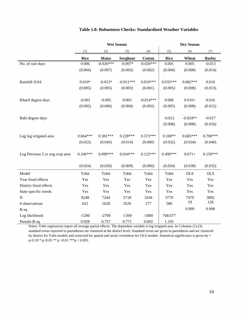
53
Wet Season Dry Season
(1) (2) (3) (4) (5) (6) (7)
Rice Maize Sorghum Cotton Rice Wheat Barley
No. of rain days 0.006 -0.026*** -0.007* -0.026*** 0.001 0.005 -0.013
(0.004) (0.007) (0.003) (0.002) (0.004) (0.008) (0.014)
Rainfall JJAS 0.010* -0.013* -0.011*** 0.010*** 0.035*** 0.062*** 0.010
(0.005) (0.005) (0.003) (0.001) (0.005) (0.008) (0.013)
Kharif degree days -0.001 -0.005 0.003 -0.014*** 0.006 0.016+ 0.016
(0.005) (0.006) (0.004) (0.002) (0.005) (0.008) (0.015)
Rabi degree days -0.012 -0.024** -0.017
(0.008) (0.008) (0.016)
Lag log irrigated area 0.664*** 0.381*** 0.228*** 0.573*** 0.100** 0.683*** 0.700***
(0.023) (0.043) (0.014) (0.000) (0.032) (0.034) (0.040)
Log Previous 5 yr avg crop area 0.106*** 0.099*** 0.034*** 0.123*** 0.499*** 0.071+ 0.150***
(0.024) (0.020) (0.009) (0.000) (0.034) (0.038) (0.032)
Model Tobit Tobit Tobit Tobit Tobit OLS OLS
Year fixed effects Yes Yes Yes Yes Yes Yes Yes
District fixed effects Yes Yes Yes Yes Yes Yes Yes
State specific trends Yes Yes Yes Yes Yes Yes Yes
N 8248 7244 5718 3244 3770 7470 3892
0 observations 632 1628 3520 277 586 19 128
R-sq
0.999 0.998
Log likelihood -1200 -2700 -1300 -1800 768.677
Pseudo-R-sq 0.928 0.757 0.771 0.692 1.105 Notes: Tobit regressions report all average partial effects. The dependent variable is log irrigated area. In Columns (1)-(3)
standard errors reported in parentheses are clustered at the district level. Standard errors are given in parenthesis and are clustered
by district for Tobit models and corrected for spatial and serial correlation for OLS models. Statistical significance is given by +
p<0.10 * p<0.05 ** p <0.01 ***p < 0.001.
Table 1.8: Robustness Checks: Standardized Weather Variables

54
*2,000 kcal per day diet.
Irrigated
agriculture
production
[million tons]
Production loss in
absence of UGW
[million tons],
(% of total production)
Calorie loss in
absence of UGW
[billion kcal]
# People fed by
UGW-dependent
calories*
[millions]
Dry Season 75.4 38.7 (51%) 121,300 166
Wet Season 73.4 2.8 (4%) 4,750 7
Annual total 148.8 41.5 (28%) 126,000 173
Table 1.9: The Impact of Unsustainable Groundwater on Irrigated Agriculture and Food Supply

55
Appendix
Fig. A.1.1: Aggregate Changes in Well and Surface Based Irrigation
Notes: Values of source-wise log irrigated area due to groundwater and surface water aggregated in each
period over the district sample are on the right axis. Groundwater includes tubewell and dug wells. Surface
irrigation includes canals and tanks. Blue bars are normalized monsoon anomalies (MA), whose values are
reported on the left axis. Agricultural data are from ICRISAT, and monsoon anomalies are from the
APHRO_MA_V1101R2 precipitation product.

56
Fig. A.1.2: Distribution of Irrigated Area
Sorghum Maize Cotton
Wheat Barley
Rice (Kharif)
Rice (Rabi)
Notes: Histogram is overlaid with an approximately scaled normal density. The normal
will have the same mean and standard deviation as the data. The blue line gives the
approximate normal distribution

57
Fig. A.1.3: Projections of Crop Irrigated Area to 2050
Notes: Econometric model generated irrigated area projections for (A) dry season and (B) wet season crops in
million hectares. The historical period (1970-2005) reflects data from ICRISAT. For the future period (2006-2050),
the solid line reflects the multi-model mean of econometric projections based on five different GCM climate futures,
with the range of uncertainty due to differences in GCM projections in the shaded region. Note that the y-axis scales
are different.
A
B

58
Fig. A.1.4: Trends in Groundwater Levels between 1979-2000 and 2029-2050 from five GCMs
Notes: Trends in groundwater levels (GWL) between 1979-2000 and 2029-2050, inferred from need for
unsustainable groundwater (UGW) to meet irrigation water demand, from 5 GCMs: A) MIROC-ESM-CHEM, B)
CCSM4, C) GFDL-CM3, D) GFDL-ESM2G, and E) NorESM1-M. Decreases in UGW demand will slow down
GWL declines (yellow); continued demand will lead to continued GWL declines (red); increase in UGW demand
will increase groundwater level (GWL) declines (dark red); relying on unsustainable sources for the first time can
start GWL declines (orange); future reliance on sustainable sources can allow GWL to recover (blue). Map has
district-level summaries, with state boundaries drawn in black. Colored (non-grey) regions account for 90% of
modeled mean national UGW demand (2029-2050).
Decreased rate of GWL declines Same rate of GWL declines Increased rate of GWL declines GWL decline begins in the future
GWL recovers/stays static
< 10% of national UGW demand
No UGW demand
Not modeled
GFDL-ESM2G NorESM1-M
MIROC-ESM-CHEM CCSM4 GFDL-CM3
A B C
D

59
Chapter 2
Water in the Balance: The Impact of Water Infrastructure on Agricultural Adaptation to
Rainfall Shocks in India
Abstract: Investments in water infrastructure remain key to climate change adaptation plans in
many countries, and rank high in adaptation costs for developing countries (Narain et al., 2011).
In this paper, we use district-level panel data from 1970-2005 across India’s major agricultural
states to investigate the role played by subsidized access to electricity, groundwater wells, tank
and dam projects in mediating the vulnerabilities associated with monsoonal variation. We focus
on wheat, a staple of India’s food supply, as it requires irrigation and represents a significant
portion of India’s total agricultural output. Results show that the impact of negative precipitation
shocks is significantly dampened when a particular district has access to a more reliable source
of irrigation – e.g., access to tubewells helps to dampen the impact of negative precipitation
shocks on irrigation decisions associated with wheat, while upstream dams do not significantly
contribute to this dampening effect. In contrast, having access to dugwells exacerbates the
impact of a fall in monsoon precipitation curtailing irrigation of wheat. Our results suggest that
historical agricultural policies that increased access to tubewells and the subsequent
electrification of regions naturally endowed with more groundwater have equipped farmers with
the ability to withstand monsoonal shocks and fluctuations.
Keywords: Water infrastructure, Adaptation, Agriculture, Irrigation, Indian Monsoon
JEL Codes: O13, Q15, Q25, Q54, Q56

60
2.1 Introduction
Given the broad scientific consensus surrounding climate change, there is a growing
concern that increased climatic variability, through its impact on agriculture, is likely to add to
the already precarious situation facing many poor households, most of whom are located in
developing countries. In India, the south-west monsoon, an atmospheric phenomenon that brings
80 percent of India’s yearly rainfall over a four-month period in summer and early fall, plays a
key role in providing the water needed to sustain agriculture as it helps to recharge rivers,
aquifers, and reservoirs (Chapter one). These rainfall realizations impact water supply, cropping
decisions, irrigation decisions, and agricultural profits, thus directly impacting the welfare of
around 770 million rural inhabitants who make up the largest share of India’s poor (World Bank,
2012). New evidence suggests that anthropogenic forcings have weakened the monsoon since the
1950s making it more erratic (Krishnan et al., 2015). Studies also project future increases in
inter-annual and intra-seasonal variability of monsoon rainfall (Menon et al., 2013).
In order to cope with such rainfall variability and smoothen the variability of water
supply, investments in water infrastructure remain key to climate change adaptation plans. For
many developing countries, water management infrastructure is ranked among the top three
categories of estimated adaptation costs (Narain et al., 2011). This is especially salient for India,
whose government has for decades promoted investments to expand irrigation as a method for
improving agricultural growth, and alleviating rural poverty (Shah, 2010). Previous research has
studied the effects of irrigation dams, and groundwater stress on rural welfare, and food
production (Duflo and Pande, 2007; Sekhri, 2013). However, there is limited research on the
potential mediating effects of different types of water infrastructure in smoothing climate
uncertainties, the consequences for irrigation water use decisions, and the spatial distribution of
these impacts. Developing such estimates is critical for India since it is the world’s most water-
stressed nation; it is also the largest agricultural and groundwater user in the world and is thus
likely to be particularly vulnerable to future changes in climate (Shah, 2010; Mendelsohn et al.,
2006).
In this paper, we use district-level panel data from 1970-2005 across 19 major
agricultural states in India to investigate the role played by subsidized access to electricity,
groundwater wells, tanks, and dam projects in mediating the vulnerabilities associated with
monsoonal variation. Specifically, we focus on the ability of these investments to reduce the

61
uncertainty associated with increased monsoonal variability by increasing access to more reliable,
yet largely unstainable sources of groundwater. We focus on wheat, a staple of India’s food
supply, as it requires irrigation and represents a significant portion of India’s total agricultural
outcomes. Our preliminary results show that the impact of negative precipitation shocks is
significantly dampened when a particular district has access to a more reliable source of
irrigation – e.g., access to tubewells helps to dampen the impact of negative precipitation shocks
on irrigation decisions associated with wheat, while upstream dams do not significantly
contribute to this dampening effect. In contrast, having access to dugwells exacerbates the
impact of a fall in monsoon precipitation curtailing irrigation of wheat.
Our results also shed light on the degree to which the introduction of an irrigation-
intensive technology (high-yielding varieties of seeds) that triggered the Green Revolution in the
mid- 1960s has influenced the evolution of irrigation infrastructure and irrigation decisions in the
period we study. Other countries have also been influenced by the evolving impacts of irrigation
access, particularly in relation to groundwater. Hornbeck and Keskin (2014) examine how
increased access to the Ogallala aquifer in the United States via improved pumps and center
pivot irrigation technology initially decreased drought sensitivity but increased drought
sensitivity over time because farmers shifted to more water-intensive crops. Given the lack of
data over a much longer historical period, we do not explicitly estimate short-run and long-run
impacts of groundwater access. However, our results illustrate how historical agricultural
policies that increased access to tubewells and the subsequent electrification of regions naturally
endowed with more groundwater- as measured by the capacity or thickness of the aquifer- have
equipped farmers with the ability to withstand monsoonal shocks and fluctuations. The results
also suggest that many of these policies may have increased the use of irrigation sources such as
non-renewable groundwater from deep tubewells, which are unlikely to be sustainable in the
long run.
Our findings provide a better understanding of how different types of water infrastructure
are likely to impact agricultural outcomes under potential water scarcity settings and shed light
on the resulting behavior of end-users of water. Such insights can also inform ongoing debates
about whether certain types of infrastructure can help with climate change adaptation
mechanisms going forward.

62
The rest of the paper is organized as follows. Section 2.2 describes the data used in the
analysis. Section 2.3 examines the path dependency of groundwater development in India.
Section 2.4 provides background on the link between different types of groundwater irrigation
technology and electricity in India. Section 2.5 assesses the impact of different types of water
infrastructure on irrigation decisions in the dry season. Section 2.6 concludes.
2.2 Data
2.2.1 Aquifers
We use the Water Resources plates (plates 88 to 92) from the 1982 National Atlas of
India , which contains hydrological maps of the presence of three categories of aquifer: thickest
(aquifer greater than 150 meters), fairly thick (aquifer thickness between 100 and 150 meters)
and thick (aquifer thickness up to 100 meters). Figure 2.1 shows the Water Resources plate (plate
88) that was used to construct measures of aquifer thickness for the northern regions of India.
We also use the World Bank India Agricultural and Climate data at the district level that reports
these variables for 124 districts. The thickness of the aquifer reflects groundwater abundance. It
does not measure the water table or annual water depth within the aquifer but captures a long
term geological potential (Jain, Agarwal and Singh, 2007).38
The thickest aquifers are under
various districts of Punjab, Haryana, and Tamil Nadu, the Green Revolution states of India, and
the fairly thick aquifers underlay Uttar Pradesh and West Bengal, other major food-producing
states in the country. Districts that are not under any of these categories have been verified to
have sporadic aquifers (Sekhri, 2014) and are not taken into account in the analysis. This
alleviates the concern that we are comparing districts with and without aquifers that differ
significantly in their hydrogeological conditions.
2.2.2 Sources of Irrigation and Electricity
The electricity data come from the Central Electric Authority’s “Public Electricity
Supply- All Indian Statistics” published annually between 1950 and 1985. We use the proportion
of villages electrified in each state in the year 1965, prior to the period of analysis39
, to allay
concerns that electrification during the sample period could also be affecting irrigation decisions.
38
While subsequent use of available groundwater could be endogenous to irrigation decisions, this measure of
groundwater availability at the outset of the period of analysis is exogenous to these decisions over time. 39
We thank Juan Pablo Rub for making these data available.

63
During the 1960s, most of the available electricity was generated within the States, and there was
negligible cross-trading of electricity (Rud, 2012). Therefore using this measure also reduces
concerns that there were spillover effects to other states.
In order to construct source-wise irrigation variables, we use data from the Land Use
Statistics Database by the Directorate of Economics & Statistics (DES), Ministry of Agriculture,
and the Village Dynamics in South Asia project at the International Crop Research Institute for
the Semi-Arid Tropics (ICRISAT). All primary statistics related to crop area, production and
irrigation are collected using land use surveys by the State governments and consolidated for the
country as a whole by the DES. ICRISAT compiles agricultural statistics from various
government sources in India including the DES, and is the only long-term publicly available
dataset of district- level statistics from 1970 to 2006. Much of the data prior to the mid-1990s is
not electronically available and is recovered from books and documents printed by the
government. We compared the source-wise irrigation data post 1998 between ICRISAT and the
online records of the Land Use Statistics Database40
to make sure the data are consistent across
the two sources.
Our dam data provide information on the number of irrigation dams constructed
both within and upstream of a district in a year, and is collected from the World Registry of
Large Dams. We draw on the data analyzed by Duflo and Pande (2007)41
to identify whether a
district is downstream or upstream from a dam. Districts that contain a dam do not generally
benefit from irrigation, due to soil salinity in surrounding areas and submergence of land
immediately surrounding the dam.42
However, regions that are downstream of a dam or in the
command area typically benefit from irrigation access (Duflo and Pande, 2007; Thakkar, 2000).
Dam construction is related to state wealth (Duflo and Pande, 2007), but since our analysis is
focused on inter-district variation any bias associated with the correlation of state wealth and
dam presence will be reduced. Further, we use the presence of an upstream dam or whether a
district is downstream from a dam at the beginning of the period of analysis to eliminate
concerns that building dams during the sample period could be affecting irrigation decisions, and
other issues related to endogenous dam placement.
40
Land Use Statistics Database’s online records begin after 1998. 41
The dataset is made available by the authors at http://hdl.handle.net/19902.I/IOJHHXOOLZ (Duflo and Pande,
2006) 42
There could be some beneficial economic activity in the reservoir area, such as fishing, but the agricultural
benefits remain limited.

64
2.3 Path-dependency of Groundwater Development
The Indian government implements a number of agricultural policies and investments
that directly or indirectly affect irrigation. The Green Revolution that introduced a new
irrigation-intensive agricultural technology in 1966-67, was one such policy initiative that was a
watershed moment in Indian agriculture.43
Figure 2.2 highlights this moment, and shows the
sharp rise in the adoption of high-yielding varieties (HYV) post 1966, with no HYV planting
prior to 1966. This rise was also accompanied by a rapid expansion of wells, particularly
tubewells , and a shift from a state- controlled surface water driven irrigation economy to one led
by private investments in groundwater infrastructure (Figure 2.3).44
This coincident rise in
groundwater irrigation was in large part because the successful adoption of HYV critically
hinged on the intensive, timely and controlled use of irrigation that groundwater sources could
provide. Irrigation through wells rose from 28 percent in 1950-51 to 62 percent in 2001-02,
largely because the share in tubewell irrigation increased from zero to over 40 percent (Gandhi,
and Namboodiri, 2009). Net area irrigated by private tubewells is about double the area irrigated
by canals .
Inherent geographical differences that influenced the variation in irrigation capacities
across regions was one of the reasons for the widespread spatial variation seen in the diffusion
and uptake of HYV seeds during the Green Revolution (Foster and Rosenzweig, 1996). For
instance, aquifer thickness, a prehistoric hydrogeological characteristic, which reflects
groundwater abundance or water endowment, influenced the variation in the types of
groundwater technology that emerged across the country. Regions that were endowed with more
groundwater due to the presence of naturally occurring thick aquifers were more suitable for
43
The focus on agricultural innovation spearheaded by the Green Revolution was in part a response to the food
crisis worsened by the consecutive droughts of the mid 1960s, and the imports of large quantities of grain. The
political leadership at that time was also pushing for a reduction in the dependence on food aid from the United
States (Evenson and Rosegrant, 1998; Dasgupta, 2014) 44
A few government run tubewell programs do exist, like the Indo Dutch Tube Well Program studied by Sekhri
(2011). However, in general, researchers have noted that the majority of India’s wells and tubewells are owned by
individual farmers (Mukherji, Rawat and Shah, 2013). Studies also note that compared to land ownership, the
distribution of well ownership is more equitable (Gandhi and Namboodiri, 2009; Mukherji, Rawat and Shah, 2013).
Small and marginal farmers with landholdings less than two hectares together owned around 67 percent of the
groundwater structures in 2005-06 even though their share of operated land was 40 percent. A majority of these
wells are financed by private investments by the farmers themselves, followed by a combination of government
subsidies, bank loans and savings. Studies also suggests that average yield on plots irrigated by private wells is
much higher than that irrigated by canals, and public tube wells (Gandhi and Namboodiri, 2009).

65
tubewell irrigation and cost-effective utilization of electric pumpsets, and thus HYV crop
cultivation (Rud, 2012).
Using this variation in aquifer thickness that is exogenous to irrigation use over time, we
estimate the time-varying effects of the introduction of the Green Revolution and spatial
variations in groundwater endowments on outcomes 𝑌𝑑𝑡 , that include HYV area, tubewell
irrigated area and dugwell irrigated area. Following in the spirit of Sekhri (2014) and Rud (2012),
we estimate the following:
𝑌𝑑𝑡 = 𝛼0 + 𝛼1𝑇ℎ𝑖𝑐𝑘𝑒𝑠𝑡𝑑 + 𝛼2𝐹𝑎𝑖𝑟𝑙𝑦 𝑇ℎ𝑖𝑐𝑘𝑑 + 𝜆𝑡 (1)
+ ∑ 𝛼1𝑡(𝑇ℎ𝑖𝑐𝑘𝑒𝑠𝑡𝑑 ∗ 𝑇𝑡) +
𝑡
∑ 𝛼2𝑡(𝐹𝑎𝑖𝑟𝑙𝑦 𝑇ℎ𝑖𝑐𝑘𝑑 ∗ 𝑇𝑡) + 𝜖𝑑𝑡
𝑡
Here, 𝑇ℎ𝑖𝑐𝑘𝑒𝑠𝑡 is an indicator that equals one if a district has access to the thickest
aquifers, and zero otherwise. Similarly, 𝐹𝑎𝑖𝑟𝑙𝑦 𝑇ℎ𝑖𝑐𝑘 is an indicator that equals one if a district
has access to fairly thick aquifers, and zero otherwise. The excluded group is the thick aquifer
category. 𝜆𝑡 are year fixed effects to capture yearly shocks, and standard errors are clustered at
the district level. The coefficients of interest are 𝛼1𝑡 and 𝛼2𝑡 where positive and significant
values indicate that districts with greater access to a particular aquifer category plant more HYV
or irrigate more via tubewells or dugwells. Increasing values of 𝛼1𝑡 and 𝛼2𝑡 imply that over time
the factors responsible for successful HYV adoption also triggered a divergence in HYV
adoption, and the type of irrigation used. We estimate the equation and plot the year-by-year
coefficients for the districts with the thickest aquifers and fairly thick aquifers relative to those
with thick aquifers in Figures 2.4, 2.5, and 2.6.
As seen in the figures, districts with greater groundwater endowments also saw higher
HYV cultivation, and higher tubewell irrigation. In contrast, districts with greater groundwater
endowments started to see a fall in dugwell irriation. Figure 2.3 shows that growth in dugwell
irrigated area remains substantially lower than tubewell irrigated area after the mid-1970s. These
patterns highlight that HYV adoption and groundwater infrastructure started to differ in areas
with higher initial groundwater endowments after the introduction of the Green Revolution.
Along with the rise in groundwater irrigation, there was a concurrent increase in demand
for electricity and electric pumpsets to access irrigation water cheaply, since other alternatives,
such as diesel pumps, were relatively more expensive (Rud, 2012). Even prior to the Green

66
Revolution, the State Electricity Boards (SEBs) had already started to introduce flat tariffs for
agricultural electricity to spur groundwater irrigation (Badiani, Jessoe and Plant, 2012). In Figure
2.7, we see that there is a rise in the share of villages electrified post 1965. The extent of
electrification increased greatly between 1966 and1979; the proportion of electrified villages
went up from 13 percent to 43.5 percent, closely following the trend in the ownership of electric
pumpsets (Barnes, 1988). By 2008, the Indian government estimated that there were 15 million
electrical pumpsets (agricultural consumers) on the grid, (Fishman et al., 2014). We run a similar
regression as above where the divergence in electrification is explained by the interaction of
aquifer thickness categories with time dummies. Instead of using district-level indicators of
aquifer thickness, we use the proportion of state area that is under the thickest or fairly thick
aquifer category, since we only have access to electricity data at the state level. Figure 2.8 plots
the year-by-year coefficients up to 1976. We see that states with greater groundwater
endowments also saw an expansion in electrification.
Overall, these patterns suggest that access to groundwater endowments enabled the
adoption of HYV which, in turn, created a demand for tubewells and rural electricity. Over time,
these characteristics that determined the successful adoption of HYV triggered a path of
divergence in the expansion of tubewell irrigation and electricity in India.
2.4 Background: Groundwater Technology and Electricity
In the following section, we highlight various characteristics of groundwater irrigation
technology that underlie the heterogeneous effects seen in the empirical analysis.
Dubash (2002) notes that there are four dimensions to groundwater irrigation technology:
accessing the water, pumping the water to the surface, the vertical location of the pump and the
power of the pump. Dugwells are the most common mode of accessing water. They are also the
shallowest, ranging in depth from 33-50 feet45
(Jain, Agarwal and Singh, 2007). Before the time
of mechanized irrigation in India, water was pumped to the surface using a traditional lift system
dependent on animal power. Later, diesel engines came to be used along with suction pumps. In
this type of setup, the engine is installed at the well mouth, and the pump is lowered down the
45
These depths can increase over time as irrigators deepen wells and lower pumps to keep pace with falling water
levels.

67
well shaft until it rests within 10 meters of the water level46
(Dubash, 2002). With the spread of
electricity to India’s villages, motors started to replace engines. In this setup, the motor is fused
together with the pump47
and placed just above the water level (Dubash, 2002).48
However, over
time, it can become increasingly unviable to adapt to falling water levels with dugwells and
suction pumps. For instance, as water levels drop, the entire well floor has to be deepened49
to
remain within the 10 meters range of the suction pump, the equipment has to be raised and the
exposed well wall has to be lined to prevent collapse, thus, considerably increasing the extent of
repair and maintenance (Dubash, 2002). Moreover, over time, the suction force of the pump
limits the extent to which water can be raised from very high depths. This is because 33 feet (or
10 meters) of water exerts a pressure of 1 atmosphere, and is the maximum height as which a
pump can suck water (Dubash, 2002; Sekhri, 2011). Since suction cannot create a perfect
vacuum, the accepted standard for vertical lift using these pumps is 25 feet (or approximately 8
meters) (Sekhri, 2011). Therefore, if the water level is beyond 25 feet or 8 meters below the
ground level, then suction pumps cannot be used to lift water.
Tubewells allow irrigators to circumvent these problems associated with increases in
pumping depths. Tubewells comprise a machine drilled tube from the ground level, an electric
powered motor and an electric submersible force pump that is lowered into the well shaft until it
rests below the water depth. The electric submersible force pump pushes water up without
relying on suction, enabling water to be pumped to any height and from far greater depths
beyond the capacities of diesel engines or electric suction pumps used in dugwells (Dubash,
2002). 50
Since tubewells, on average, have larger pumps, it is also possible to extract greater
yields of water. Shallow tubewells can range in depth from 50-70 feet, and in sedimentary
formations can go as deep as 230 feet, providing roughly two to three times the water available
from a dug well (Jain, Agarwal and Singh, 2007). Deep tubewells are drilled to depths of 300-
500 feet and provide fifteen times the water available from a dug well (Jain, Agarwal and Singh,
46
Suction pumps are limited by the height air pressure can lift a column of water and so must be located no more
than about 10 meters from the water source 47
In the engineering literature, this is referred to as ‘monoblock’ 48
The motor can also be placed on the dry bed of the dugwell, such that water is sucked out using a hand drilled
bore. Hence, this type of well is also called dug-cum-bore well). In general, such technology is difficult to maintain
since it is located at the bottom of the well. 49
Dugwell depths can go as deep as 150 feet. 50
When farmers switch from low cost surface pumps to much more expensive submerged pumps as depths increase,
the overall fixed cost of pumping increases at one (or more) discrete point(s) (Sekhri, 2011), even with subsidized
electricity.

68
2007). Even if water levels fall in tubewells, submersible pumps can be easily lowered to access
water.51
Tubewells are, therefore, technically able to provide assured long-term access to
groundwater even in times of drought, and also greater volumes of water.52
2.5 Heterogeneous Effects
In this section, we use the variation in irrigation infrastructure and electricity provision
initiated by the Green Revolution as well as natural groundwater endowments to understand their
role in diminishing or amplifying the influence of precipitation shocks on crop irrigation
decisions in the dry season. We focus on wheat since it is the predominant irrigation-intensive
crop grown in the dry season.
2.5.1 Empirical Model and Results
We split the districts into those that fall under thickest, fairly thick and thick aquifers, and
re-estimate the model from Chapter one to compare how areas with different factor (water)
endowments influence adaptation of agriculture to weather shocks. The sample size is relatively
small since we only cover districts that have information about aquifer thickness or initial
groundwater endowments. The following model is estimated separately for each sample of
districts:
log 𝑌𝑑,𝑡 = 𝛾0 + 𝛼 𝑙𝑜𝑔𝑌𝑑,𝑡−1 + 𝛽 𝑙𝑜𝑔 𝑹𝒅,𝒕 + 𝛾1𝑙𝑜𝑔𝐺𝐷𝐷 + 𝛾2𝑙𝑜𝑔𝐴𝑑,𝑡−1,𝑡−6 + 𝜌𝑑 + 𝜆𝑡 + 𝐴𝑠,𝑡
+ 𝜖𝑑,𝑡
As discussed in section 2.3, factor endowments have played a role in influencing the
types of irrigation infrastructure and capacities that have developed in India. Therefore, we
expect that precipitation shocks will not impact districts that overlay the thickest aquifers.
Results in Table 2.1 show that, as expected, for districts overlaying the thickest aquifers,
irrigation in the dry season is completely buffered from monsoon rainfall shocks, and monsoon
rainfall no longer impacts wheat irrigation. For districts that overlay fairly thick and thick
aquifers, however, the impact of monsoon rainfall is positive and significant, such that the
51
Over time, however, discharge rates could decrease if the pump is made to extract water from even greater depths 52
Shah and Kishore (2009) explain that the dugwell irrigated southern regions in India were affected relatively more
than the tubewell irrigated northern states during the 2002 drought that followed below normal rainfall in 2000 and
2001.

69
magnitude of the coefficient on monsoon rainfall is significantly lower for regions with access to
fairly thick aquifers (100-150 meters) relative to those with access to thick aquifers (≤ 100
meters). These results reflect the differential processes of electrification and tubewell irrigation
in places with higher groundwater endowments as illustrated in section 2.3.
In Table 2.2, we examine whether better access to the benefits of groundwater in districts
that experienced a higher process of electrification, can help mediate rainfall shocks. Since
electrification enables the use of electric pumps for groundwater extraction, we interact total
precipitation with a dummy for states whose share of electrified villages was greater than the
national average in 1965 in Column (1) of Table 2.2. We use the share of electrified villages at
the outset of the Green Revolution and a little before our sample period to allay the concern that
electrification during the sample period could also be affecting irrigation decisions. We find a
significant impact of electrification mediating the adverse effects of a negative rainfall shock on
wheat irrigated area. In columns (2) and (3), we interact total precipitation with share of
electrification as well as a dummy for whether a district overlays the thickest or fairly thick
aquifer. The excluded group is the thick aquifer category. As expected, we find that the
mediating effect of electrification is even stronger in districts with access to the thickest aquifers
(Column (2)).
Next, we examine the impacts of different types of irrigation infrastructure on mitigating
or amplifying monsoon rainfall shocks. In Columns (4)-(6) , we interact total monsoon
precipitation with dummies identifying districts whose proportions of tubwell, dugwell and tank
irrigated area (normalized by district area) are above the national average. Consistent with
section 2.4, we find that tubewells mediate the impact of a fall in monsoon precipitation on
wheat irrigation, in contrast to dug wells and tanks. The coefficients on the monsoon
precipitation variable and the interaction of monsoon rainfall with the tubewell indicator variable
have opposite signs, and remain statistically significant in columns (4) - (6). On the other hand,
dugwells amplify the effect of a monsoon rainfall shock. The coefficients on the monsoon
precipitation variable and the interaction of monsoon rainfall with the dugwell indicator variable
have the same sign, and are statistically significant (Columns (5) and (6)). Overall, the results
suggest that access to deep groundwater plays a fundamental role in mediating negative rainfall
shocks and supporting irrigation in the dry season.
Even as the Green Revolution provided an impetus to the rise of wells, public

70
investments in dams continued. The Government built 3000 large dams53
between 1947 and
2001 (Pande, 2008), using 80 percent of its direct irrigation outlays for major and medium
irrigation54
projects towards their construction (Vaidyanathan, 2010; Taraz, 2015). Since dams
supply surface water to downstream districts, we identify districts that have upstream dams.
Since dam placement is likely endogenous to the extent of irrigation, we use indicator variables
to classify downstream districts using information about presence of upstream dams from 1970
or the beginning of our sample period. This prevents concerns about dam presence during the
sample period also affecting irrigation coverage. Results are reported in Column (7) of Table 2.2.
We see that districts that are downstream are able to mediate the effect of a fall in precipitation
since the interaction term between the downstream indicator and monsoon precipitation is
negative; however this effect is not significant.
2.5 Conclusion
The results of this analysis demonstrate that access to different types of irrigation
infrastructure can significantly dampen or exacerbate the role that monsoonal variation plays on
irrigation decisions along the extensive margin.
The results also show that policies enacted during the Green Revolution that increased
access to more reliable sources of irrigation have been vital in mediating the impact of
monsoonal uncertainties – especially for dry-season crops like wheat. For instance, agricultural
policies related to tubewell expansion and electrification, have been especially vital in
determining the extent to which monsoonal rainfall variation impacts dry- season irrigation.
Our results also suggest that many of these policies may have increased the use of
irrigation sources that may not be sustainable in the long run. While groundwater irrigation
clearly provides an economic and social benefit via access to a more reliable source of irrigation,
the fact that these resources are non-renewable in many regions of the country makes their use as
an irrigation resource largely unsustainable in the long run.
53
A large dam is defined as a dam having a height of 15 meters from the foundation, or, if the height is between 5
and 15 meters, having a reservoir capacity of more than 3 million cubic meters (Duflo and Pande, 2007) 54
Major (medium) irrigation projects are defined as those with a command area larger than 10,000 (2000) hectares.

71
References
Badiani R., K.K. Jessoe and S. Plant (2012) Development and the environment: the implications
of agricultural electricity subsidies in India, The Journal of Environment & Development 21(2):
244-262
Barnes, D. F. (1988) Electric power for rural growth: how electricity affects rural life in
developing countries, Rural Studies Series
Dasgupta, A. (2014) Why Dominant Parties Decline: Evidence from India’s Green Revolution,
Working Paper
Dubash, N. K. (2002) Tubewell capitalism: groundwater development and agrarian change in
Gujarat. Oxford University Press, New Delhi
Duflo, E. and R. Pande (2007) Dams, Q. J. Econ., 122(2):601-646
Evenson, R. E.and M.W. Rosegrant (1998) Agricultural Research and Productivity Growth in
India. Vol. 109 International Food Policy Research Institute.
Fishman, R. U. Lall, V. Modi and N. Parekh (2014) Can Electricity Pricing Save India's
Groundwater? Evidence from Gujarat, Working Paper
Foster, A. D. and M. R. Rosenzweig (1996) Technical change and human-capital returns and
investments: evidence from the Green Revolution, American Economic Review, 931-953.
Gandhi, V.P. and Namboodiri, N.V. (2009) Groundwater irrigation in India: Gains, costs, and
risks. Ahmedabad, India: Indian Institute of Management
Hornbeck, R., and P. Keskin (2014) The historically evolving impact of the ogallala aquifer:
Agricultural adaptation to groundwater and drought, American Economic Journal: Applied
Economics, 6(1), 190-219.
Jain, S., P. Agarwal, and V. Singh (2007) Hydrology and Water Resources of India, Water
Science and Technology Library, Springer
Krishnan, R., T. P. Sabin, R. Vellore, et al. (2015) Deciphering the desiccation trend of the South
Asian monsoon hydroclimate in a warming world, Clim. Dynam. 1-21
Mendelsohn, R., A. Dinar, and L. Williams (2006). The distributional impact of climate change
on rich and poor countries, Environ. Dev. Econ, 11(02):159-178

72
Menon, A., A. Levermann, J. Schewe, J. Lehmann and K. Frieler (2013) Consistent increase in
Indian monsoon rainfall and its variability across CMIP-5 models. Earth Sys. Dynam. 4(2): 287-
300
Mukherji, A., S. Rawat, and T. Shah (2013) Major Insights from India’s Minor Irrigation
Censuses: 1986-87 to 2006-07, Economic & Political Weekly, 48(26): 115-124.
Narain, U., S. Margulis, and T. Essam (2011) Estimating costs of adapting to climate change,
Clim. Policy, 11: 1001–1019
Rud, J. P. (2012) Electricity provision and industrial development: Evidence from India, Journal
of development Economics, 97(2): 352-367
Sekhri, S. (2011) Public provision and protection of natural resources: Groundwater irrigation in
rural India, American Economic Journal: Applied Economics, 29-55.
Sekhri, S. (2013) Missing Water: Agricultural Stress and Adaptation Strategies in response to
Groundwater Depletion among Farmers in India, Working Paper
Sekhri, S. (2014) Wells, Water, and Welfare: The Impact of Access to Groundwater on Rural
Poverty and Conflict. Am Econ J Appl Econ 6(3):76-102.
Shah, T. and A. Kishore (2009) Will the Impact of the 2009 Drought Be Different from 2002?"
Economic and Political Weekly, 11-14.
Shah, T. (2010) Taming the Anarchy: Groundwater Governance in South Asia, Resources for the
Future Press, Washington DC
Taraz, V. (2015) Adaptation to Climate Change: Historical Evidence from the Indian Monsoon,
Yale University Working Paper
Thakkar, H. (2000) Assessment of Irrigation in India. World Commission of Dams
Vaidyanathan, A. (2010) Agricultural Growth in India: The Role of Technology, Incentives, and
Institutions, Oxford University Press India
World Bank (2012) India: Issues and Priorities for Agriculture, available from:
http://www.worldbank.org/en/news/feature/2012/05/17/india-agriculture-issues-priorities

73
Figures
Fig 2.1 Aquifer capacity in northern India
Notes: The map illustrates Plate 88 from the 1982 National Atlas of India

74
0
50000
100000
150000
200000
250000
1956 1959 1962 1965 1968 1971 1974 1977 1980 1983 1986
Area under HYV
0
10
20
30
40
50
60
1970 1972 1974 1976 1978 1980 1982 1984 1986 1988 1990 1992 1994
Tubewell irrigated area Dugwell irrigated area
Fig 2.2 Trends in area under High Yielding Varieties (HYV)
Notes: Area is measured in hectares. Data is from the Indian Agriculture and Climate
Dataset, World Bank.
Fig 2.3: Trends in irrigated area by different sources
Notes: Area is measures in 1000 hectares. Data is from ICRISAT and Directorates of
Economics and Statistics, Ministry of Agriculture.

75
0
20000
40000
60000
80000
100000
120000
140000
160000
180000
200000
19
57
19
59
19
61
19
63
19
65
19
67
19
69
19
71
19
73
19
75
19
77
19
79
19
81
19
83
19
85
19
87ye
ar b
y ye
ar r
egr
ess
ion
co
eff
icie
nts
fo
r H
YV
are
a
Thickest aquifers > 150 m Fairly Thick aquifers 100-150m
0
10
20
30
40
50
60
70
80
90
19
71
19
72
19
73
19
74
19
75
19
76
19
77
19
78
19
79
19
80
19
81
19
82
19
83
19
84
19
85
19
86
19
87ye
ar b
y ye
ar r
egr
ess
ion
co
eff
icie
nts
fo
r tu
be
we
ll ir
riga
ted
are
a
Thickest aquifers> 150m Fairly Thick aquifers 100-150m
Fig 2.4: Differential trends in area under High Yielding Varieties ( HYV) by aquifer capacity
Notes: Area is measures in hectares. Data is from the Indian Agriculture and
Climate Dataset World Bank, and National Atlas of India
Fig 2.5: Differential trends in tubewell irrigated area by aquifer capacity
Notes: Area is measures in 1000 hectares. Data is from ICRISAT, Directorates of
Economics and Statistics, Ministry of Agriculture, and National Atlas of India.

76
0
0.1
0.2
0.3
0.4
0.5
0.6
0.7
0.8
19
61
19
62
19
63
19
64
19
65
19
66
19
67
19
68
19
69
19
70
19
71
19
72
19
73
19
75
19
76
19
78
19
79
19
80
19
81
19
82
19
83
Share of Villages electrified
-50
-45
-40
-35
-30
-25
-20
-15
-10
-5
0ye
ar-b
y-ye
ar r
egr
ess
ion
co
eff
icie
nts
fo
r d
ugw
ell
irri
gate
d a
rea
Thickest aquifer > 150 m Fairly Thick aquifer 100-150 m
Fig 2.6: Differential trends in dugwell irrigated area by aquifer capacity
Notes: Area is measures in 1000 hectares. Data is from ICRISAT, Directorates of
Economics and Statistics, Ministry of Agriculture, and National Atlas of India.
Fig 2.7: Trends in electrification
Notes: Data is from the Central Electric Authority.

77
0
0.1
0.2
0.3
0.4
0.5
0.6
0.7
0.8
1968 1969 1970 1971 1972 1973 1975 1976
year
by
year
re
gre
ssio
n c
oe
ffic
ien
ts
for
shar
e o
f vi
llage
s e
lect
rifi
ed
Thickest aquifer > 150 m
Fairly Thick aquifers 100-150 m
Fig 2.8: Differential trends in electrification by aquifer capacity
Notes: Data is from the Central Electric Authority, and National Atlas of India
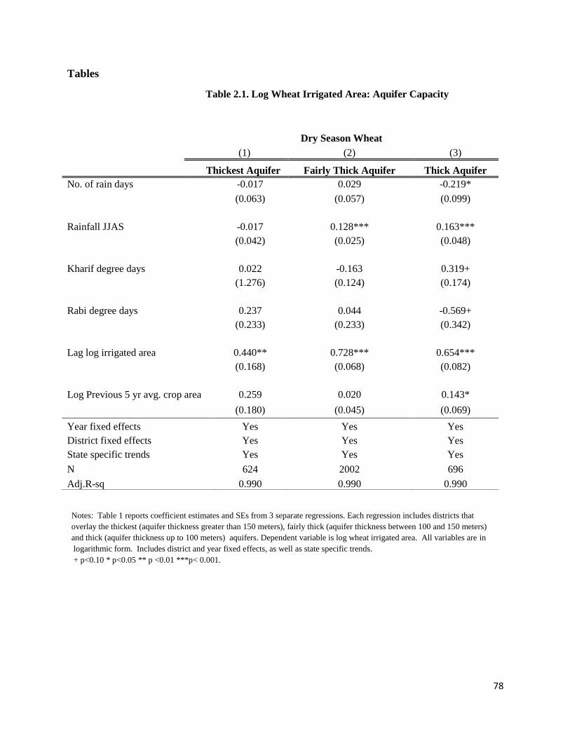
78
Tables
Notes: Table 1 reports coefficient estimates and SEs from 3 separate regressions. Each regression includes districts that
overlay the thickest (aquifer thickness greater than 150 meters), fairly thick (aquifer thickness between 100 and 150 meters)
and thick (aquifer thickness up to 100 meters) aquifers. Dependent variable is log wheat irrigated area. All variables are in
logarithmic form. Includes district and year fixed effects, as well as state specific trends.
+ p<0.10 * p<0.05 ** p <0.01 ***p< 0.001.
Table 2.1. Log Wheat Irrigated Area: Aquifer Capacity
Dry Season Wheat
(1) (2) (3)
Thickest Aquifer Fairly Thick Aquifer Thick Aquifer
No. of rain days -0.017 0.029 -0.219*
(0.063) (0.057) (0.099)
Rainfall JJAS -0.017 0.128*** 0.163***
(0.042) (0.025) (0.048)
Kharif degree days 0.022 -0.163 0.319+
(1.276) (0.124) (0.174)
Rabi degree days 0.237 0.044 -0.569+
(0.233) (0.233) (0.342)
Lag log irrigated area 0.440** 0.728*** 0.654***
(0.168) (0.068) (0.082)
Log Previous 5 yr avg. crop area 0.259 0.020 0.143*
(0.180) (0.045) (0.069)
Year fixed effects Yes Yes Yes
District fixed effects Yes Yes Yes
State specific trends Yes Yes Yes
N 624 2002 696
Adj.R-sq 0.990 0.990 0.990

79
Notes: Column (1) reports the baseline model without interactions. Column (2) -(7) include interactions of total rainfall with dummies for states with higher electrification in 1965
relative to national average, for districts overlaying thickest and fairly thick aquifers, for districts dominated by tubewells, dug wells, and tanks, for districts that have upstream dams in
1970. Standard errors reported in parentheses are corrected for spatial and serial correlation. Statistical significance is given by + p<0.10 * p<0.05 ** p <0.01 ***p < 0.001.
Dry Season Wheat
(1) (2) (3) (4) (5) (6) (7)
No. of rain days -0.005 -0.072 -0.064 -0.032 -0.062 -0.055 -0.055
(0.071) (0.072) (0.072) (0.071) (0.070) (0.069) (0.069)
Rainfall JJAS 0.250*** 0.387*** 0.344*** 0.404*** 0.310*** 0.294*** 0.324***
(0.034) (0.049) (0.040) (0.043) (0.040) (0.046) (0.055)
Rainfall JJAS x electricity -0.262***
(0.052)
Rainfall JJAS x electricity x thickest aquifer -0.359***
(0.044)
Rainfall JJAS x electricity x fairly thick aquifer -0.282***
(0.043)
Rainfall JJAS x high tubewells -0.371*** -0.339*** -0.331*** -0.344***
(0.043) (0.040) (0.043) (0.047)
Rainfall JJAS x high dugwells 0.198*** 0.206*** 0.211***
(0.048) (0.047) (0.051)
Rainfall JJAS x high tanks 0.057 0.076
(0.058) (0.059)
Rainfall JJAS x upstream dam 1970 -0.054
(0.052)
Kharif degree days 0.089 0.155 0.136 0.096 0.098 0.101 0.101
(0.069) (0.105) (0.104) (0.104) (0.103) (0.103) (0.103)
Rabi degree days -0.159 -0.329+ -0.249 -0.172 -0.181 -0.183 -0.186
(0.099) (0.185) (0.184) (0.180) (0.177) (0.177) (0.178)
Fixed Effects District, Year, State-Year Time Trends
N 7460 6847 6812 6847 6847 6847 6847
Adj.R-sq 0.990 0.999 0.999 0.999 0.999 0.999 0.999
Table 2.2. Log Wheat Irrigated Area: Heterogeneous Effects

80
Chapter 3
The Impact of Water Access on Short-term Migration in Rural India
Abstract: This chapter examines the impacts of irrigation water access, availability and use on
labor mobility in rural India. Using nationally representative household-level survey data
combined with district- specific weather, irrigation, groundwater and electricity data, it
investigates the role that water infrastructure and groundwater development have played in
influencing short-term migration, a common and economically important mechanism by which
rural households diversify their income sources. Results show that migration decisions respond
to agricultural opportunity costs associated with irrigation and that access to assured irrigation
determines the relative benefits of migration. Tubewells, especially deep tubewells, allow
farmers and laborers to profitably farm lands even in times of rainfall scarcity and this benefit
lowers the degree of temporary migration. Further, our results show that higher electricity
provision lowers the likelihood of short-term migration, even in areas where depths to
groundwater have consistently fallen. This suggests that regions with access to electricity have
been able to adapt and shift to new technologies that facilitate continued pumping. From a
policy perceptive, shutting down access to groundwater will significantly increase temporary
labor mobility.
Keywords: Short-term migration, Groundwater, Irrigation, Electricity, Indian Monsoon
JEL Codes: D74, I32, O13, O15, Q15, Q16
81
3.1 Introduction
Scientists anticipate that the effects of climate change on the hydrological cycle, while
still largely uncertain, are likely to be strikingly uneven across time and space as changes in
climate patterns will change the water balance at many places (World Bank, 2016). Since
developing countries have limited ability to adapt to such changes, the effects might be more
pronounced in these regions. Increasing water scarcity is likely to affect agricultural economies
the hardest, affecting hundreds of millions of smallholder farmers in semi-arid, developing
countries who depend on irrigation for their livelihoods (Vorosmarty et al., 2000). The Indian
subcontinent, with its diverse socioeconomic and climatic conditions, is particularly vulnerable
to changes in precipitation patterns (Turner and Annamalai, 2012). In recent decades, the
monsoon circulation has weakened and precipitation has declined (Singh et al., 2014); a trend
that scientists have largely attributed to anthropogenic forcing (Krishnan et al., 2015). Such
changes in monsoon variability can have direct impacts on agriculture (as noted in Chapter one)
as well as far reaching effects on the overall economy.
Studies have projected that water scarcity and climate change could uproot millions
(Parry et al., 2007; Brown, 2008; Mundial, 2009; Warner, 2010), making “water refugees”, and
“hydrological poverty” commonplace in semi-arid areas (Brown, 2012). Past ethnographic
studies have documented out-migration from areas in India where access to water is limited
(Chopra and Gulati, 2001; Moench, 2002; Prakash, 2005; Nair and Chattopadhyay, 2005).55
More recently, reports of people migrating from villages as a result of drought have been
grabbing headlines.56
However, an empirical understanding of how rural households and
individuals respond to multiple dimensions of water scarcity is still limited, especially in relation
to labor mobility. In this chapter, we focus on how rural individuals’ decisions to temporarily
migrate in India are influenced by climatic factors, and irrigation water access, availability and
use.
Irrigation is a critical source of adaptation by which India combats the impact of rainfall
variability, smoothens agricultural production risk, and improves food security. Chapter one
55
Even as far back as the Holocene period 8,000 years BC, archaeological evidence shows that populations migrated
eastward where rainfall was sufficient in response to extended periods of drought and weakening of the monsoon
(Gupta et al., 2006). 56
Vidhi Doshi, “India's drought migrants head to cities in desperate search for water”, The Guardian, April 27, 2016
“Government may record migration from drought-hit villages”, Times of India, Feb 23, 2014; “Drought forcing
villagers to migrate from Rajasthan border district”, Business Standard, Oct 14, 2014
82
highlighted the relationship between monsoon rainfall and irrigation in India. Results indicated
that farmers responded to water scarcity along the extensive margin by adjusting the extent of
cultivated and irrigated area seasonally from year to year. Other studies have also found evidence
of Indian rural households adapting over longer time frames by investing in irrigation in response
to past periods of low rainfall (Taraz, 2014). Much of India’s irrigation is dependent on
groundwater use, and although certain areas are facing falls in groundwater levels, groundwater
continues to remain the most prominent and important source of irrigation. Therefore, reduced
access to groundwater resources is a constraint on agricultural livelihoods and fundamental to
water scarcity in rural India. Chapter two explained the salience of the relationship between
aquifer properties, irrigation technology and water levels from the past to the present. India’s
heterogeneous hydrogeological landscape underlies the scale at which water is available. The
thickness of the aquifer captures groundwater storage capacity which, in turn, influences the risk
perception and investment decisions of farmers. This, in turn, affects the type of water extraction
technologies that emerge, and the likely institutional and ownership forms that result. As water
levels begin to drop, irrigation technology has to be constantly modified to keep pace. This can
also affect the scale of irrigation unexpectedly; as the size of pump necessary to access the water
from greater depths increases, the extent of irrigation also rises with greater yields of water
(Dubash, 2002). In this chapter, we investigate the spillover effects of these interactions and
changes in water access on labor mobility.
Using nationally representative household-level survey data combined with district-level
weather, irrigation, groundwater level and electricity data, this study examines short-term
migration, a common and economically important mechanism by which rural households,
especially those with small and marginal landholdings, diversify their income sources.57
While
papers have described rural Indians as relatively immobile compared to similarly developing
countries (Munshi and Rosenzweig, 2009)58
, this is largely reflective of low rates of permanent
migration in existing data. In post-independence India, land markets have been thin. Hence
permanent migration, for reasons other than marriage, is rare. On the other hand, labor migration
57
Lanjouw and Shariff (2004) have shown that rural households can have highly varied and often multiple sources
of incomes to self-insure and reduce the variance of household income in response to risk, especially risks related to
low agricultural productivity. 58
Munshi and Rosenzweig (2009) develop a theory of caste networks to explain low levels of permanent migration
of males form their home villages. Other studies have based their analysis of different policies like trade
liberalization (Topalova, 2010) on the assumption that labor is immobile in their models.

83
from Indian villages is common, and a large portion of this migration is for short lengths of
time.59
Short-term migration, is an “irreversible part of the livelihoods of rural communities”
(Mosse et al., 2002), and is central to a long-term economic strategy that provides a diversified
source of income60
to sustain rural livelihoods, and cope with risks (Stark, 1982), particularly
risks associated with aggregate weather related shocks (Badiani and Safir, 2010). Results show
that migration decisions respond to agricultural opportunity costs associated with irrigation and
that access to assured irrigation determines the relative benefits of migration. Tubewells,
especially deep tubewells, allow farmers and laborers to profitably farm lands even in times of
rainfall scarcity and this benefit lowers the chance of temporary migration. Moreover, results
also indicate that the likelihood of temporary migration decreases from regions which
consistently face deeper groundwater levels, as long as electricity distribution is more developed
in these areas. This suggests that an increase in electrification facilitates the use of electric pumps
for groundwater extraction and enables farmers to adapt or invest in technology that allows
access at even greater depths. Therefore, better access to the benefits of groundwater as a result
of higher electricity provision increases the agricultural focus of households, and significantly
lowers short-term migration. Maintaining access to groundwater is, thus, an important lever in
sustaining rural livelihoods.
This paper contributes to two strands of previous literature in economics. First, it
contributes to the small but growing literature on environmental migration. While a number of
economic models have been developed to study migration over the past 50 years61
, only recently
59
Short-term or temporary migration is well documented in the literature (Haberfield et al., 1999; Mosse et al., 2002;
Banerjee and Duflo, 2007; Deshingkar et al., 2009; Badiani and Safir, 2010; Keshri and Bhagat, 2012; Coffey, Papp
and Spears, 2014; Morten, 2014). For a detailed case study of patterns of labor migration in India,
see Breman (1996). For prevalence of temporary migration in other developing countries refer to de Brauw
and Harigaya (2007) (Vietnam); Macours and Vakis (2010) (Nicaragua); Bryan, Chowdhury and Mobarak
(2013)(Bangladesh). 60
Some studies also call this type of migration as one that “diversifies distress” between seasons of low and high
agricultural productivity (Basu and Kashyap, 1992) 61
Primarily, four key models have been put forward. The Hicks-Sjaastad Model (Sjaastad, 1962) argues that
migration is driven by wage differentials, so that migration takes place if life-time benefits of living in a new
location outweigh the one time migration cost. Todaro (1969) modifies this model to put forth the idea that
migration is a function of expected income differences in rural (origin) and urban area (destination) adjusted by the
probability of gaining employment in the urban sector, so that the move takes place if the expected benefits
outweigh the cost. Both these models are motivated for long term migration. The New Economics of Labor
Migration (NELM) framework put forth by Stark and Levhari (1982) and Stark and Bloom (1985) take into account
the role of risk aversion and the role of the household as a decision making unit. Here households use migration as a
tool to diversity their portfolio of risk across members, especially when there are missing markets for credit,
insurance, etc as is normally the case in a developing country setting. Finally, in the last class of models, workers
base their relocation on the trade- off between utility they might receive from wages and from other attributes of the

84
have economists started to estimate the causal interactions between environmental change and
migration. In developing countries, the effects of gradual changes62
in climate and weather
variability have been shown to affect migration through the wage channel (Marchiori et al.,
2012), or through the agricultural productivity channel (Feng et al., 2010). Unlike developed
countries, the direct migration response to the amenity value of climate is significantly lower due
to income rigidities in developing countries (Klaiber, 2014).63
There is limited empirical evidence about migration due to environmental factors in
India. Studies that have examined the impacts of environmental change on mobility within India
have focused on permanent migration based on state-level migration data from Census data
(Dallmann and Millock, 2013; Viswanathan and Kumar, 2012) or household data from smaller
geographical areas within a state (Fishman, Jain and Kishore, 2015). Dallmann and Millock
(2013) find that inter-state migration rises marginally in response to an increase in drought
frequency and Viswanathan and Kumar (2015) finds some evidence for inter-state migration in
response to weather changes, via the channel of falling wheat and rice yields. A recent study by
Fishman, Jain and Kishore (2015) marks a significant departure from previous studies, and is the
first to empirically study permanent male migration in response to groundwater depletion, in the
context of a gradual well-anticipated environmental change in India. However, their focus is
geographically limited in scope since they focus on two districts in the north-western state of
Gujarat that have already experienced very large declines in groundwater levels. They also do
not extend their analysis to other forms of migration that are economically more important for
many small and marginal farmers. The study uses deep-lying geological features that are
hydrologically responsible for an increase in the fall of water tables to distinguish between water
scarce and water abundant villages. They find that for the water scarce villages there are higher
locations (environmental amenities), and the cost of migration. These equilibrium sorting models provide direct
estimates of preferences and can help with simulating and predicting behavioral responses (Klaiber, 2014) 62
Instead of gradual changes in the climate, some studies have focused on environmental shocks: Hornbeck (2012)
and Hornbeck and Naidu (2014) investigate impacts on local economies that are affected by sudden environmental
shocks within the United States. Hornbeck (2012) finds that populations affected by a sudden and severe period of
drought and soil erosion in the 1930s adapted through out-migration, and not through adjustments within other
sectors (agriculture and industry). Hornbeck and Naidu (2014) find significant out-migration of blacks in counties
affected by the Great Mississippi Flood of 1927.
63
In countries like the United States, however, these effects are substantial. Rappaport (2007) examines the direct
effect of weather amenities on migration in the US, and finds that households migrate to places with warmer winters
and cooler summers even after controlling for sectoral employment.
85
rates of permanent male migration to urban areas from households that belong to a relatively
richer landholding class. Sekhri (2013), on the other hand, uses data on all districts in India and
finds that there is no evidence that depletion of groundwater below eight meters, the cutoff at
which fixed cost of extraction increases, causes any change in the number or area of
landholdings under various size groups. The author notes that this indicates that there is no
evidence of exit of marginal or small farmers from agriculture. Therefore, further understanding
of the evolving impacts of water stress on different types of labor mobility in India is still needed.
This paper attempts to fill this gap by focusing on short-term migration, the predominant form of
labor migration that underlies the livelihood strategies of India’s small and marginal farmers.
This paper also contributes to the literature on consumption smoothing in response to
aggregate shocks.64
In general, aggregate shocks are more difficult to insure against than
idiosyncratic shocks. In India, the amount of monsoon rainfall and associated farm income
variability remains the main source of risk and uncertainty that a rural household faces. Since
insurance, capital and futures markets are either absent or incomplete in India, like in much of
the developing world, short-term migration serves as a coping mechanism in periods of low
agricultural productivity (Reardon, et al., 2006).
Previous research on India has provided evidence of risk management and coping in
response to aggregate shocks through labor markets (Rose, 2001; Ito and Kurosaki, 2009).65
Migration, as one such strategy, has also been studied. Rosenzweig and Stark (1989) explain
how spatial risk diversification might be one mechanism by which households smooth
consumption. They study marriage migration across six villages in India and find that households
are able to mitigate spatially covariant risks and smooth consumption ex ante since they arrange
marriages with households located a greater distance apart where weather shocks are unlikely to
be highly correlated. Using revised data from the same set of six villages, Badiani and Safir
(2010) find that in addition to spatial risk diversification, households also engage in ex post
64
The majority of the development economics literature has examined idiosyncratic shocks at the household level,
and not aggregate shocks (Deaton, 1997; Udry,1994)
65
Rose (2001) finds that households who face less reliable rainfall are more likely to participate in the labor market
(an ex ante response). Furthermore, when they are actually faced with a negative rainfall shock, households respond
with increases in days of labor. Ito and Kurosaki (2009) focus on households in two northern states of Uttar Pradesh
and Bihar using the Living Standards Measurement Survey data from the year 1997-98. They find that higher
rainfall variability reduces the labor share on on‐farm activities and increases the shares of non‐farm activities and
in‐kind farm work.

86
temporal risk diversification. Their results show that temporary or short-term migration- which is
not a result of patrilocal exogamy- rises substantially in response to aggregate village-level
weather shocks. New evidence that uses independent survey data on migration from 60 villages
across three north-west states of Rajasthan, Gujarat and Madhya Pradesh also finds that short-
term migration serves to diversify risk across definite time periods or agricultural seasons when
aggregate weather affects agricultural productivity the most (Coffey et al. 2014). Our study
contributes to the existing literature by drawing inferences about the relationship between
climatic conditions, different types of adaptation ( irrigation and short-term migration) and the
extent to which ex ante investments in irrigation infrastructure impact ex post adaptation
strategies. In particular, we investigate how higher agriculture opportunity costs as reflected in
irrigation access, might affect the likelihood of temporary migration by household members. The
study covers all of rural India with its diverse agro‐ecological zones, and varying irrigation
capacities, and therefore is not limited by the specificity of the sample and geographical region.
Migration is a complex phenomenon and environmental change is one of many reasons
that can contribute to migration especially in a country that is facing rapid economic and social
change. Therefore, we do not attempt to suggest that water access is the only driver for migration.
However, given the risk posed by climate change to rural and agrarian communities, it is
necessary that we understand how behavior and decision-making respond to changes in water
availability, particularly with respect to short-term migration that occupies a large proportion of
migration in the country.
The rest of the paper is organized as follows. Section 3.2 develops a conceptual
framework to illustrate the impact of water access on migration decisions in an agrarian
economy. Section 3.3 describes the data and provides contextual information on short-term
migration, irrigation, groundwater levels and electricity provision. Section 3.4 presents our
empirical strategy and results. The robustness checks are presented in Section 3.5, and our
conclusions are presented in Section 3.6. Descriptions of the modeling assumptions used in our
conceptual framework are explained in the Appendix.
3.2 Conceptual Framework
We motivate our study of migration decisions in response to environmental change and
water availability using a simple two-period model of irrigation investment and migration. Our

87
model builds on Rosenzweig and Binswanger (1993), a seminal paper on agricultural risk and
investment decisions in India. Literature on developing countries has emphasized the risk-averse
nature of households and farmers. These studies point to ex ante self-insuring, as well as ex post
income smoothing decisions in the absence of credit and insurance markets (Kochar, 1999;
Jayachandran, 2006).
Following past studies, we consider a risk-averse farm household made up of N members
that is also an expected utility maximizer. For simplicity, we assume that the household has
preferences over consumption given by a mean-variance utility function with 𝛽 > 0 representing
an Arrow-Pratt coefficient of absolute risk aversion.66
We also assume no access to credit and
insurance markets.
The representative household maximizes 𝐸[𝑈(𝑐)] = 𝑉[𝜇𝑐, 𝜎𝑐2] = 𝜇𝑐 −
𝛽
2𝜎𝑐
2, where 𝜇𝑐
and 𝜎𝑐2 are the mean and variance of consumption such that 𝑉𝑢 = 1, 𝑉𝜎2 = 𝛽/2, 𝑉𝜇𝜇, 𝑉𝜎2𝜎2 and
𝑉𝜇𝜎2 = 0, 𝑉𝜇𝜇𝑉𝜎2𝜎2 − 𝑉𝜇𝜎2 ≥ 0. Utility is maximized over 𝜇𝑐 and minimized over 𝜎𝑐2.
From this 𝑁 extended household, 𝑛 migrate, so that the fraction who migrate are 𝜃 =𝑛
𝑁 and
the fraction who don't are 1 − 𝜃 = 1 −𝑛
𝑁. The household's production function is given by
𝑓(𝛼, 𝜃, 𝑒) where 𝛼 represents investments in irrigation assets, such that 𝑓𝛼 < 0 at the margin and
𝑓𝜃 < 0 since we assume that the farm is managed by the extended household and there is no
hired labor. 𝑒 represents exogenous electricity provision and is a productivity shifter such that
𝑓𝑒 > 0 . Additionally, the variability of production on farm is given by Γ(𝛼, 𝜃, 𝑒) such that
Γ𝛼 < 0, Γ𝜃 > 0 and Γ𝑒 < 0 following from the same assumptions.
Income per person on the farm is given by 𝑊𝑓(𝛼, 𝜃, 𝑒)𝑤 where 𝑊 is the total wealth
endowment of the household adjusted by a factor of farm output and key random weather
variables in each period 𝑤 ∈ (𝑤1, 𝑤2), where 𝑤1 is rainfall in period one and 𝑤2 is temperature
in period two.67
On the other hand, the income of the person who migrates is given by 𝑚 − 𝑐 ,
where 𝑚 is the income earned on migrating and 𝑐 is the migration cost.
A given agricultural year in India starts from June of the current year to May of the
following year. On average, the monsoon or the wet season begins in June and continues through
66
Specifically, we consider a constant absolute risk aversion utility function, 𝑈(𝐶) = −𝑒−𝛽𝑐 , so that 𝐸[𝑈(𝐶)] =
𝐸[−𝑒−𝛽𝑐] = 𝜇𝑐 −𝛽
2𝜎𝑐
2 under normally distributed consumption. 67
Rainfall is negligible in period two.
88
September of the same calendar year, the winter season begins in October and continues to
February of the next calendar year and summer lasts from end of February to May. In our model,
period one represents the monsoon season, and period two represents the winter and summer
seasons (or the dry season). Eighty five percent of the annual rainfall occurs between June and
September, at a time when major crops such as rice are grown. Though the monsoon starts to
withdraw post September, it has lasting effects in the subsequent months as it replenishes water
supply in irrigation canals, tanks, reservoirs and wells (see Chapters one and two). Irrigation is,
therefore, extremely important for agricultural productivity in the winter and summer months.
In the model, we assume that the household invests in irrigation assets, 𝛼1, during period
one, and a fraction of the household, 𝜃2 , migrates in period two. The implicit assumption
underlying the model, is that migration 𝜃2 occurs only in period two, but households make
contingency plans for migration in period one given by 𝜃2𝑐. Output 𝑦1(𝛼1, 𝑤1, 𝑒) is realized after
period one and output 𝑦2(𝛼1, 𝜃2, 𝑤2, 𝑒)is realized after period two. Once 𝑦1 is realised, we
assume that there are no savings, such that 𝑦1 = 𝑐1. From these assumptions, if follows that:
𝐸0[𝑤1] = 𝜇𝑤1, 𝑉0[𝑤1] = 𝜎𝑤1
2 , 𝐸0[𝑤2] = 𝜇𝑤2, 𝑉0[𝑤2] = 𝜎𝑤2
2 , 𝐸1[𝑤2] = 𝜇𝑤2∗ and 𝑉1[𝑤2] = 𝜎𝑤2
2∗ .
The timing of the events is as follows:
1. Choose 𝛼1 and 𝜃2𝑐 given 𝐸0[𝑤1], 𝑉0[𝑤1], 𝐸0[𝑤2], 𝑉0[𝑤2], 𝑊, 𝑚 − 𝑐
2. 𝑤1 and 𝑦1 are realized
3. Choose 𝜃2 given 𝐸1[𝑤2], 𝑉1[𝑤2], 𝑤1, 𝛼1, 𝑦1, 𝑊, 𝑚 − 𝑐
4. 𝑤2 and 𝑦2 are realized.
The household consumption for periods 1 and 2 is given by:
𝐶 = 𝑊𝑓1(𝛼1, 𝑒)𝑤1 + (1 − 𝜃2𝑐)𝑊𝑓2(𝛼1, 𝜃2𝑐 , 𝑒)𝑤2 + 𝜃2𝑐(𝑚 − 𝑐)
𝜃1 = 0
Therefore,
𝜇𝑐 = 𝑊𝑓1(𝛼1, 𝑒)𝜇𝑤1+ (1 − 𝜃2𝑐)𝑊𝑓2(𝛼1, 𝜃2𝑐 , 𝑒)𝜇𝑤2
+ 𝜃2𝑐(𝑚 − 𝑐)
𝜎𝑐2 = 𝑊Γ1(𝛼1, 𝑒)𝜎𝑤1
2 + (1 − 𝜃2𝑐)𝑊Γ2(𝛼1, 𝜃2𝑐 , 𝑒)𝜎𝑤22
Given the above consumption function, the household maximizes the following in period one:

89
𝐸0[𝑈(𝐶)] ≈ 𝑉[𝜇𝑐, 𝜎𝑐2] w.r.t 𝛼1, 𝜃2𝑐
This gives us optimal amounts of 𝛼1∗(𝜇𝑤1
, 𝜎𝑤12 , 𝜇𝑤2
, 𝜎𝑤22 , 𝑊, 𝑚 − 𝑐, 𝑒) and
𝜃2𝑐∗ (𝜇𝑤1
, 𝜎𝑤12 , 𝜇𝑤2
, 𝜎𝑤22 , 𝑊, 𝑚 − 𝑐, 𝑒).
After period one, there still remains uncertainty about period two output 𝑦2 and temperature 𝑤2.
However, the household now faces updated estimates of 𝜇𝑤2∗ and 𝜎𝑤2
2∗ than what they expected at
the beginning of period one.
Household consumption in period two is given by:
𝐶2 = (1 − 𝜃2)𝑊𝑓2(𝛼1, 𝜃2, 𝑒)𝑤2 + 𝜃2𝑐(𝑚 − 𝑐)
Therefore,
𝜇𝑐2= (1 − 𝜃2)𝑊𝑓2(𝛼1, 𝜃2, 𝑒)𝜇𝑤2
∗ + 𝜃2𝑐(𝑚 − 𝑐) + 𝑦1
𝜎𝑐2 = (1 − 𝜃2)𝑊Γ2(𝛼1, 𝜃2, 𝑒)𝜎𝑤2
2∗
Again, the household maximizes:
𝐸1[𝑈(𝐶)] ≈ 𝑉[𝜇𝑐2, 𝜎𝑐2
2 ] w.r.t 𝜃2
This gives us an optimal value of 𝜃2∗( 𝜇𝑤2
∗ , 𝜎𝑤22∗ , 𝛼1, 𝑊, 𝑚 − 𝑐, 𝑒).
Given the model and the underlying assumptions, we are interested in the sign of 𝜕𝜃2
𝜕𝛼1 and
𝜕𝜃2
𝜕𝑒 =
𝜕𝜃2
𝜕𝑒 |𝛼1 +
𝜕𝜃2
𝜕𝛼1
𝜕𝛼1
𝜕𝑒 , both of which we expect to be < 0. We expect that a rise in irrigation
decreases the extent of migration. In turn, we expect that a rise in electrification that spurs
irrigation will also decrease the extent of migration. In an area where irrigation is very important,
the opportunity cost of staying when there is no access to irrigation is presumably high. In other
words, on-farm labor and irrigation can act as complements for mean consumption (𝜕2𝜇𝑐2
𝜕𝜃2𝜕𝛼1< 0).
With more capital assets in irrigation, and a lower percent of assets in other forms of capital such
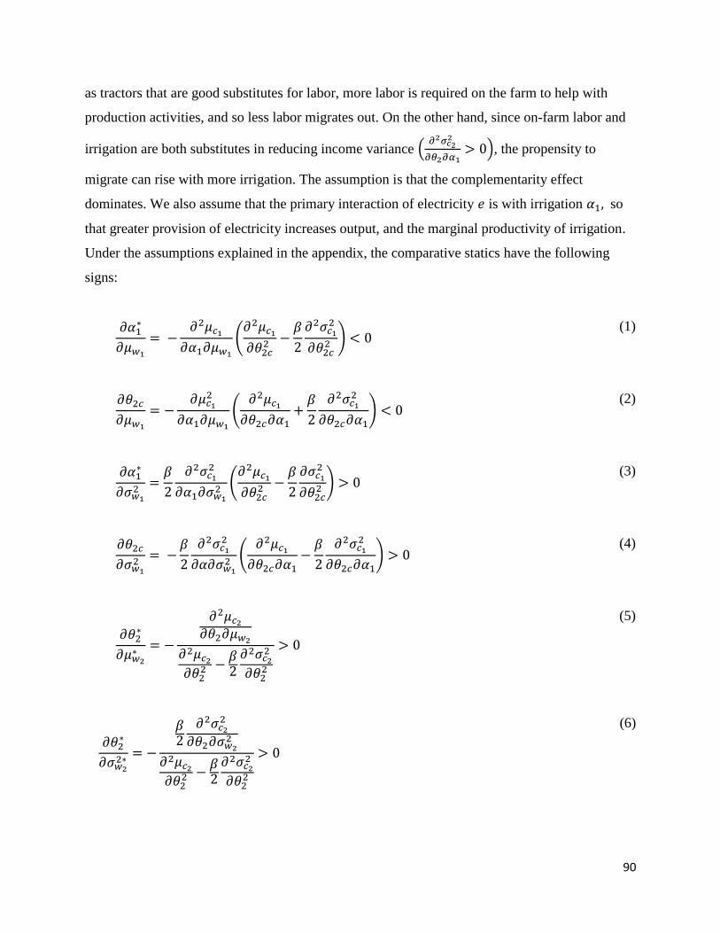
90
as tractors that are good substitutes for labor, more labor is required on the farm to help with
production activities, and so less labor migrates out. On the other hand, since on-farm labor and
irrigation are both substitutes in reducing income variance (𝜕2𝜎𝑐2
2
𝜕𝜃2𝜕𝛼1> 0), the propensity to
migrate can rise with more irrigation. The assumption is that the complementarity effect
dominates. We also assume that the primary interaction of electricity 𝑒 is with irrigation 𝛼1, so
that greater provision of electricity increases output, and the marginal productivity of irrigation.
Under the assumptions explained in the appendix, the comparative statics have the following
signs:
𝜕𝛼1∗
𝜕𝜇𝑤1
= −𝜕2𝜇𝑐1
𝜕𝛼1𝜕𝜇𝑤1
(𝜕2𝜇𝑐1
𝜕𝜃2𝑐2 −
𝛽
2
𝜕2𝜎𝑐12
𝜕𝜃2𝑐2 ) < 0
(1)
𝜕𝜃2𝑐
𝜕𝜇𝑤1
= −𝜕𝜇𝑐1
2
𝜕𝛼1𝜕𝜇𝑤1
(𝜕2𝜇𝑐1
𝜕𝜃2𝑐𝜕𝛼1+
𝛽
2
𝜕2𝜎𝑐12
𝜕𝜃2𝑐𝜕𝛼1) < 0
(2)
𝜕𝛼1∗
𝜕𝜎𝑤12
=𝛽
2
𝜕2𝜎𝑐12
𝜕𝛼1𝜕𝜎𝑤12
(𝜕2𝜇𝑐1
𝜕𝜃2𝑐2 −
𝛽
2
𝜕𝜎𝑐12
𝜕𝜃2𝑐2 ) > 0
(3)
𝜕𝜃2𝑐
𝜕𝜎𝑤12
= −𝛽
2
𝜕2𝜎𝑐12
𝜕𝛼𝜕𝜎𝑤12
(𝜕2𝜇𝑐1
𝜕𝜃2𝑐𝜕𝛼1−
𝛽
2
𝜕2𝜎𝑐12
𝜕𝜃2𝑐𝜕𝛼1) > 0
(4)
𝜕𝜃2∗
𝜕𝜇𝑤2∗
= −
𝜕2𝜇𝑐2
𝜕𝜃2𝜕𝜇𝑤2
𝜕2𝜇𝑐2
𝜕𝜃22 −
𝛽2
𝜕2𝜎𝑐22
𝜕𝜃22
> 0
(5)
𝜕𝜃2∗
𝜕𝜎𝑤22∗
= −
𝛽2
𝜕2𝜎𝑐22
𝜕𝜃2𝜕𝜎𝑤22
𝜕2𝜇𝑐2
𝜕𝜃22 −
𝛽2
𝜕2𝜎𝑐22
𝜕𝜃22
> 0
(6)
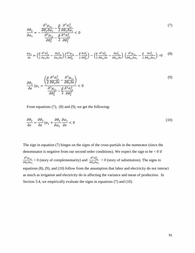
91
𝜕𝜃2
𝜕𝛼1= −
𝜕2𝜇𝑐2
𝜕𝜃2𝜕𝛼1−
𝛽2
𝜕2𝜎𝑐22
𝜕𝜃2𝜕𝛼1
𝜕2𝜇𝑐2
𝜕𝜃22 −
𝛽2
𝜕2𝜎𝑐22
𝜕𝜃22
< 0
(7)
𝜕𝛼1
𝜕𝑒= (
𝛽
2
𝜕2𝜎𝑐12
𝜕𝛼1𝜕𝑒−
𝜕𝜇𝑐12
𝜕𝛼1𝜕𝑒) (
𝜕2𝜇𝑐1
𝜕𝜃2𝑐2 −
𝛽
2
𝜕𝜎𝑐12
𝜕𝜃2𝑐2 ) − (
𝛽
2
𝜕2𝜎𝑐12
𝜕𝜃2𝑐𝜕𝑒−
𝜕𝜇𝑐12
𝜕𝜃2𝑐𝜕𝑒) (
𝜕2𝜇𝑐1
𝜕𝜃2𝑐𝜕𝛼1−
𝛽
2
𝜕𝜎𝑐12
𝜕𝜃2𝑐𝜕𝛼1) >0
(8)
𝜕𝜃2
𝜕𝑒|𝛼1 =
(𝛽2
𝜕2𝜎𝑐22
𝜕𝜃2𝜕𝑒−
𝜕2𝜇𝑐2
𝜕𝜃2𝜕𝑒)
𝜕2𝜇𝑐2
𝜕𝜃22 −
𝛽2
𝜕2𝜎𝑐22
𝜕𝜃22
< 0
From equations (7), (8) and (9), we get the following:
(9)
𝜕𝜃2
𝜕𝑒 =
𝜕𝜃2
𝜕𝑒 |𝛼1 +
𝜕𝜃2
𝜕𝛼1
𝜕𝛼1
𝜕𝑒< 0
(10)
The sign in equation (7) hinges on the signs of the cross-partials in the numerator (since the
denominator is negative from our second order conditions). We expect the sign to be < 0 if
𝜕2𝜇𝑐2
𝜕𝜃2𝜕𝛼1 < 0 (story of complementarity) and
𝜕2𝜎𝑐22
𝜕𝜃2𝜕𝛼1 > 0 (story of substitution). The signs in
equations (8), (9), and (10) follow from the assumption that labor and electricity do not interact
as much as irrigation and electricity do in affecting the variance and mean of production. In
Section 3.4, we empirically evaluate the signs in equations (7) and (10).

92
3.3 Data and Context
Our empirical analysis integrates individual level short-term migration data from a
nationally representative survey with weather station data, and district-level68
water access data
that focuses on irrigation infrastructure, electricity coverage and groundwater levels.
3.3.1 National Sample Survey (NSS) Migration Data
In general, there is a paucity of reliable migration data in India. This is especially true of
short-term migration which occupies an important share of migration in the country, but lacks
proper documentation in official Census statistics.
In this paper, our primary source of information is the National Sample Survey
Organization’s nationally representative socio-economic survey on employment, unemployment
and migration conducted from July 2007 to June 2008 across 35 states and union territories.
This 64th
round of the NSS is the only richest source of migration till date69
covering the
migration history of each household member. It is stratified by urban and rural areas of each
district. The survey covers close to 79,000 rural and 46,000 urban households, and provides
details about approximately 374,000 rural and 197,000 urban individuals. This paper focuses on
rural areas, since we are interested in the impacts of rural water infrastructure on short-term
migration out of these source regions. Moreover, short-term migration is especially widespread
in rural India. According to the NSS 2007-08 survey, 12.58 million rural residents were short-
term migrants, in comparison to one million urban residents. The lowest geographical unit in the
68
Districts are administrative units within states that resemble counties in the United States, and are a commonly-
used unit for planning. Most government agencies, therefore, have detailed data at the district level. The average
district area of 5000 sq. km. supports an average population of two million. This is roughly twice the average area of
a U.S. county (2,584 sq. km.), and nearly 18 times greater than the average population of a U.S. county (100,000).
69
Other nationally representative datasets that cover migration information are the Census, REDS (Rural Economic
and Demographic Survey), and an earlier NSS survey from the year 1999-2000. However, they do not provide
comprehensive migration information to the extent that the NSS 2007-08 round does. For instance, the Census only
provides information about in-migrants, not out-migrants or short-term migrants, and captures information at the
state level with only a subset of indicators at the district level. The 2006 survey data from REDS contains seasonal
migration information, but markedly underestimates the extent of such migration in the country. In the REDS survey
only 0.25 percent migrate in the wet season, 0.31 percent migrate in the winter and 0.35 percent migrate in the
summer. In contrast, an independent survey of short-term migrants in 70 villages across a high migration area
overlapping the borders of three states, Rajasthan, Gujarat and Madhya Pradesh, found these estimates to be in the
range of 10%, 29% and 35% in the wet, winter and summer seasons respectively(Coffey et al., 2014). The NSS
1999-2000 survey uses a slightly different definition as to what constitutes a short-term migrant and underestimates
the extent of short-term migration. It also contains no information about the number of such trips, or the destination,
details that are included in the NSS 2007-08 survey.
93
survey for rural India is a village and the survey covers 7,984 villages, from which households
are selected based on a stratified multistage design.70
Our sample includes districts within
twenty six states, excluding the state of Jammu and Kashmir since survey data is missing due to
conflicts in the region. The remaining 552 districts represent 98% of the population of India.
Certain households are over-sampled, and therefore the NSSO provides sampling weights (see
National Sample Survey Organisation (2010) for more details), which we use to adjust all
statistics used in the paper.
Short-term Migration
Most migration related literature has focused on how immobile the Indian population is
using data focusing on permanent migration flows (Munshi and Rosenweig, 2009). Short-term
migration, on the other hand, is both common and economically important.
The 64th round of the NSS for the year 2007-08 is the first survey to capture to some
extent the breadth and scale of short-term migration in India. It captures short-term migration by
asking whether each household has spent between one and six months away from the village for
work during the last 365 days.71
It further records the number of migration trips, the industry in
which they worked during these trips, and the destination they went to during the longest spell.
The destination could either be within the same district (rural or urban), in another district in the
same state (rural or urban) or in another state (rural or urban).72
Additionally, household and
demographic characteristics, socio-economic particulars, and employment status of individuals
prior and post migration are also recorded in detail. Overall, short-term migrants made up 1.7
percent of the rural population, 2.51 percent of rural prime age adults and 80 percent of all rural
out-migrants. Figure 3.1 shows the spatial distribution of short-term migrants in India. Of all the
70
Households are chosen from the village based on the following criteria: (1) two households having at least one
out-migrant and received at least one remittance from him/her during the last 365 days, (2) four households among
the remaining households having at least one other type of migrant, including temporary out-migration for
employment, and (3) four other households (National Sample Survey Organization, 2010). 71
The only other NSS survey that has captured short term migration is the NSS 1999-2000 survey but with a
different definition. NSS 1999-2000 asks whether each household member has spent between two and six months
away from the village for work within the past year. For this reason, 2007-08 data reports higher levels of short-term
migration than 1999-2000. 72
The destination could also be to another country, but the percentage of such short-term migrants in the data is
extremely low at less than 0.6 percent.
94
rural households, 5.8 percent or 9.25 million have at least one short-term migrant (Table 3.1).
Despite the staggering numbers, it is likely that even this estimate is an under-estimate.73
In our analysis, we restrict the sample to inter-district short-term migrants that
temporarily move to another district within the same state, or to another state, so that we can
measure the impact of source-specific district characteristics on temporary movements away
from the district. Moreover, the majority of short-term migrants are inter-district and not intra-
district migrants. Table 3.1 shows that less than 20 percent of short-term migrants move intra-
district, while nearly 80 percent of them move inter-district. Most rural short-term migrants are
more likely to migrate to urban areas than rural areas; 58.43 percent of short-term migrants move
to urban areas of another district (Table 3.1).
Certain households might have fewer short-term migrants as a result of past migration
histories of households. If households permanently sorted to locations with better water
availability and irrigation infrastructure 40 years ago at the time of the Green Revolution, then it
is possible that fewer household members are short-term migrants today. Table 3.1 shows that
this is unlikely. More than 84 percent of short-term migrants have always resided in the place of
enumeration, and only two percent come from households that moved to the place of
enumeration 30 to 40 years ago. Therefore, we are capturing short-term migration movements
that are unlikely to have been influenced by permanent migration decisions made at an earlier
time.
The NSS household data does not provide the precise location of the sampled villages.
Therefore, the district is the lowest administrative level at which we can link the NSS 2007-08
survey to other datasets.
3.3.2 Irrigation Data
The NSS 2007-08 survey provides us detailed information on migrants, but lacks
irrigation and agricultural information of households. The most comprehensive and detailed data
available for irrigation in India is the Minor Irrigation Census (MIC) conducted by the Ministry
73
The counting of short-term migrants is a contentious issue in India. Many argue that official statistics
underestimate the magnitude, and this is corroborated by independent surveys (Coffey et al., 2014) that find higher
short-term migration rates. The reasons for this discrepancy are the way households are defined and the time frame
used to define a short-term migrant. As per the NSS survey, a household comprises a group of people who live
together and share a common kitchen, excluding guests, visitors and all those who stay away from the household for
more than 6 months. However, some who stay away for more than 6 months and reside at home for the rest of the
months are still technically part of the household and could potentially be termed short-term migrants
(Chandrasekhar et al., 2014).

95
of Water Resources, Government of India on a quinquennial basis. We make use of data from the
2006-07 round. The other three rounds are for the years 1986-87, 1993-94 and 2000-01. The
MIC accounts for the entire population of groundwater structures and surface water schemes.
The data includes information about area irrigated by different sources (surface schemes,
tubewells- shallow and deep, and dug wells), as well as sown area, cultivated area, average depth
of the water table, among other variables. We match district level variables from the MIC to
districts included in the NSS 2007-08 migration survey.
3.3.3 Electricity Data
Ideally, we would use household level variables on electricity access and supply for all
migrant households. Since such information is absent in the NSS 2007-08 survey, two other
sources of electricity coverage are used. We make use of the Village Directory from the 2001
Census, as well as satellite nighttime lights data for the year 200174
to construct district-level
measures of electrification.
Census Data:
The Village Directory constitutes 96 variables on a wide range of village-level amenities
for all inhabited villages in the country, and is the only source that provides detailed information
at the level of a village, the smallest administrative unit in India. Among the various amenity
data like schools, health facilities, banking facilities, source of drinking water, and transportation
infrastructure, it also includes data on electricity supply, and if such supply is available for
agricultural, domestic or other purposes. Unfortunately, these village level infrastructure data
cannot be matched with the villages of the NSS households, since village level identifiers are not
publicly disclosed in the NSS data. Therefore, using this information, we construct district-level
variables using district boundaries that correspond to the 2001 Census and compute the fraction
of villages with electricity supply for agricultural purposes in each district.
Nightlights Data:
We also use a novel dataset of satellite images of the earth at night. Many recent studies
have used nighttime lights data as a proxy for economic activity arguing that brightness is highly
correlated with GDP (Henderson et al., 2012; Bleakley and Lin, 2012; Storeygard, 2013; Sigman
74
The NSS 2007-08 migration survey follows the sample frame of the 2001 Census. We also use nighttime lights
for the year 2006 in robustness checks.

96
and Olmstead, 2016). In this paper, however, we exploit the fact that there is a physical
relationship between consumption of electricity and nighttime lights, making the nightlights a
good proxy for electrification, even at small spatial scales (Elvidge et al., 1997; Chand et al.,
2009; Min, 2011; Min et al., 2013; Min and Gaba, 2014).75
The satellite night lights data comes from the United States Air Force Defense
Meteorological Satellite Program’s operational Linescan System (DMSP-OLS)76
that comprises
a set of satellites flying in polar orbit since 1970 recording high resolution images of all locations
on earth every night between 20:00 and 21:30 local time from an altitude of 830 kilometers
above the earth. Since 1992, these images have been digitized and used widely by the scientific
community. The most commonly used data are a series of annual composite images, although
daily images are also available. The annual composite images are created by overlaying images
from a calendar year, dropping images where lights are masked by cloud cover or overpowered
by the effects of auroral lights or solar glare (near the poles), and by excluding late-evening
sunlight due to longer days in the summer months as well as removing ephemeral lights like
fires , noise, other temporary lighting phenomena and irregularities (Min, 2011; Elvidge et al.,
1997). The final series are a set of stable night light images for all locations on the earth starting
from 1992 (Elvidge et al. 1997). These images are processed by the National Oceanic and
Atmospheric Agency's (NOAA) National Geophysical Data Center (NGDC). Each DMSP-OLS
satellite generates pixels that are 30 arc-seconds long (approximately 0.86 square kilometers at
the equator) which can be aggregated to any scale, jurisdictional unit and geographic area.77
Each
pixel is coded from zero to 63, a value that is proportional to the average observed luminosity
(Henderson et al., 2012).78
75
Studies have shown that nighttime brightness can be used to detect electrification status. Elvidge et al. (1997)
found high correlations between nighttime light output and electricity use at the national level. Min et al. (2013)
show that nighttime brightness can reliably detect electrified villages in Senegal and Mali making it a useful proxy
for electricity provision in the developing world. Min and Gaba (2014) find that a similar relationship between
electrification and nighttime brightness exists in rural Vietnam. Chand et al. (2009) show a direct relationship
between nighttime lights and electric power consumption in India, while Min (2011) finds a strong correlation
between brightness and district-level electricity consumption in Uttar Pradesh, a northern state in India. 76
Nighttime lights data are available for download at http://ngdc.noaa.gov/eog/dmsp/downloadV4composites.html 77
Examples in the literature include nations, provinces, states, local government areas, grids of 1° latitude × 1°
longitude and even smaller units. 78
Fig 3.2b shows an image of 2001 stable nighttime lights in India. The very brightly lit area in the upper left is
New Delhi, the capital of India. The state’s large cities are clearly visible. At the same time, areas with large swathes
of darkness with no detectable light emissions are also seen. Satellite images are consistently collected across space,
and therefore the areas of darkness are not a result of satellites not being able to detect low levels of light. In fact,
many thousands of villages emit detectable levels of light that are not visible on the printed page. Therefore, pixels

97
Using GIS software, we overlay a shapefile of district boundaries over annual composite
images and construct average annual indicators of nighttime light output for each district by
summing the light values of all pixels within the district for a given year. In years where more
than one satellite is in orbit, we average the pixel values across the two sensors.
3.3.4 Groundwater Level Data
We make use of district level data from the Central Groundwater Board of India for the
years 2005-2009.79
The data provide information from approximately 16000 monitoring wells in
the country, that record groundwater measurements four times in a year- in the pre-monsoon
months of January and May, and in the monsoon and post-monsoon months of August and
November. The wells are fairly evenly spread across India, but exclude the hilly regions in the
north and north-east. The groundwater level data are aggregated to the district level using district
boundaries corresponding to the 2001 Census, and we use annual average district-level data in
the empirical analysis.
3.3.5 Groundwater Levels and Electricity Access
Chapter two pointed out the salience of the relationship between aquifer properties, water
levels, and irrigation technology from the past to the present. In the subsequent section, we
explain the interactions between groundwater levels and electrification.
In general, the optimal use of groundwater requires equating the marginal benefit of
water with the cost of pumping plus a user cost that represents the future loss of benefits due to
depletion and the increase in pumping cost associated with a depleted stock. In India, user costs
are rarely paid, and in most cases the full pumping cost also remain unpaid. Most regions in
India receive electricity subsidies and there is widespread use of electrical pumps. Electricity
supply to agriculture is free in states like Tamil Nadu, Andhra Pradesh and Maharashtra, while in
other states farmers pay a heavily subsidized flat electricity tariff that is based on the horse-
power rating of the pump rather than actual consumption.80
The flat rates are partly because the
electricity use is related to pump size. With substantially large subsidies, the marginal cost of
that are lit for one village and unlit for another similar village do in fact suggest presence of electrical infrastructure,
availability and use of electricity (Min, 2011) 79
This was the only data available for all districts in India. Information on groundwater levels for a longer time
series can be acquired with permission, and results in the paper will be updated on receiving this data. 80
Subsidies are under the jurisdiction of the state electricity board. State Electricity Boards (SEBs) are responsible
for transmission, distribution and generation of electricity, as well as the setting and collection of tariffs (Badiani,
Jessoe, and Plant, 2012)

98
pumping reduces drastically. This leads to a higher than optimal extraction rate of groundwater.
When farmers pay little (or in some cases, even zero) at the margin for electricity used for
pumping, all available electricity will be used for groundwater pumping. Jessoe and Badiani
(2015) provide causal evidence that electricity subsidies have led to increases in groundwater
extraction, and also in the probability of groundwater exploitation in India. They find that a one
rupee increase in the monthly fixed rate per horsepower of electricity leads to a 1.05 million
cubic meter decrease in groundwater extraction.
With a rise in groundwater extraction in excess of recharge, water levels start to fall
(Chapter one). Information about the distribution of villages into different groundwater level
categories is available in two rounds of the MIC census, in the years 1993-94 and 2000-
01.81
Figure 3.3 shows that the percentage of villages with higher depths to groundwater82
(greater than ten meters) has been increasing over time. On the other hand, the percentage of
villages with lower depths to groundwater (less than ten meters) has been falling over time. To
address the risk of falling water tables farmers have adapted by shifting to new technologies.
Access to electricity has enabled farmers to shift to more expensive technology, like submersible
electrical pumps and tubewells that allow groundwater to be pumped from even greater depths.
The MIC shows that for India as a whole, the number of electric pumps increased from 4.7
million in 1986-87 to almost 10 million in 2000-01 accounting for 54 percent of the total pumps
in the country, double the increase in growth seen for diesel pumps.
Underlying these national estimates is a stark regional dimension to electricity access,
and, in turn, in the use of electrical pumps for pumping groundwater. Panel A of Figure 3.2 maps
the percentage of villages that receive electricity for agricultural purposes from the 2001 census,
and panel B of Figure 3.2 maps the geographic distribution of nightlights in 2001. The striking
variation in electricity access between the east and the rest of India is apparent across both
datasets. While states in the peninsular region, north and northwestern states have access to
subsidized electricity supply, paradoxically eastern parts of India that receive the highest amount
of rainfall, and do not suffer drops in ground water levels, are faced with limited rural electricity
supply. In these regions, farmers who attempt to use electricity to pump water have to face a
much higher flat tariff, and need to get permission from multiple state and village level bodies to
81
MIC did not collect groundwater depth information for villages in the 2006-07 census round. 82
Depth to groundwater is the mean depth from surface to where groundwater is first observed.

99
receive electricity connections (Mukherji et al., 2009). Therefore, most famers in the east
continue to use diesel, and have to bear the high sticky marginal cost of pumping (given the lack
of subsidies), which in turn has inhibited groundwater use (Mukherji, Rawat and Shah, 2013).
Consequently, farmers have better access to the benefits of groundwater in regions where
electricity distribution is more developed, since electricity provision facilitates the use of electric
pumps for groundwater extraction.
Using groundwater level data from the Central Groundwater Board of India, we map
districts where depth to groundwater has stayed over eight meters (red) or under eight meters
(grey) over the five years for which data is available in Figure 3.5. Chapter two highlighted that
beyond a certain water table threshold of eight meters, farmers shift to more expensive
technology to access water, thus facing a discrete jump in the rise of pump cost (Sekhri, 2011).
We see that the regions shaded in red coincide with regions that also receive greater electricity
supply. These patterns are consistent with a scenario in which electricity provision, and subsidies
have not only increased but also facilitated continued groundwater use despite falls in
groundwater levels by allowing farmers to shift to new technologies. Therefore, while the Green
Revolution heralded a private tubewell revolution, more recently, there has been a rise in deep
tubewell irrigation (Figure 3.4). According to the second MIC round of 1993-94, around 80
percent of the deep tubewells were privately owned. By the third MIC round of 2000-01, 90
percent of the deep tubewells became privately owned (Mukherji, Rawat and Shah, 2013).83
In summary, electricity provision has triggered greater groundwater use in India and, in
turn, the adoption and expansion of tubewells, and a recent notable rise in deep tubewell
irrigation. In the following section, we estimate how these attributes of groundwater
development impact labor mobility.
83
In general, researchers have noted that the majority of India’s wells and tubewells are owned by individual
farmers (Mukherji, Rawat and Shah, 2013). Studies also note that compared to land ownership, the distribution of
well ownership is more equitable (Gandhi and Namboodiri, 2009; Mukherji, Rawat and Shah, 2013). Small and
marginal farmers with landholdings less than two hectares together owned around 67 percent of the groundwater
structures in 2005-06 even though their share of operated land was 40 percent. MIC data shows that a majority of
these wells are financed by private investments by the farmers themselves, followed by a combination of
government subsidies, bank loans and savings. Studies also suggests that average yield on plots irrigated by private
wells is much higher than that irrigated by canals, and public tube wells (Gandhi and Namboodiri, 2009).

100
3.4 Empirical Approach and Results:
To measure the impacts of irrigation technology, electricity access, groundwater levels,
and weather on short-term migration, we estimate the following linear probability model (LPM):
𝑀𝑖ℎ𝑑 = 𝑓(𝑊𝑑, 𝐼𝑑,𝐸𝑑 𝐺𝑑; 𝛽𝑤, 𝛽𝑖, 𝛽𝑒 , 𝛽𝑔) + 𝛿1𝑍𝑑 + 𝛿2𝐺𝑖ℎ𝑑 + 𝛿3𝐾ℎ𝑑 + 𝜂𝑡 + 𝜇𝑠 + 𝜖𝑖ℎ𝑑
(21)
Here, 𝑀𝑖ℎ𝑑 is a binary variable that takes on the value of one if an individual 𝑖 in
household ℎ living in district 𝑑 is an inter-district short-term migrant during the time of the
survey, and zero otherwise. The regressors of interest are a function of weather 𝑊𝑑, irrigation
𝐼𝑑 , electricity 𝐸𝑑, and groundwater levels 𝐺𝑑 in district 𝑑. We include averaged annual growing
degree days (GDD) and monsoon rainfall over a 30 year period from 1975-2005 for all districts.
These long- term averages over 30 years are referred to as normal. In addition, as a covariate risk
factor, we include a rainfall shock measure to capture the ex post response of off-farm labor
supply to production shocks. This variable is calculated as the deviation of rainfall in 2006 (the
year immediately prior to the NSS survey) from normal rainfall. We include a range of irrigation
technology variables at the district level: the percentage of cultivated area that is irrigated by
wells or surface water, and further the percentage of cultivated area that is irrigated by deep
tubewells, shallow tubewells and dugwells.84
We use both the fraction of villages with electricity
supply for agricultural purposes, and the log of nighttime light output per square kilometer for
each district as electricity measures. A limitation in using our key irrigation and electricity
provision variables at the district level is that they do not capture household heterogeneity within
a district. At the same time, since our key variables are measured at the district-level, concerns
about endogeneity bias are reduced.
We include a number of household controls 𝐾ℎ𝑑 : landholding size (<1 hectare, 1.01- 4
hectares, > 4 hectares), log of monthly per capita expenditure (MPCE), and household size.
MPCE is calculated using the total average value of goods and services a household consumes
per month, and is often used as a proxy for household income (National Sample Survey
Organization, 2010).85
The amount of land owned represents household assets or wealth which
84
Instead of focusing on the spread and number of wells, we use area irrigated by different types of wells to make
sure we capture actual utilization along with access, and not just access. 85
As it is difficult to collect reliable income data, the National Sample Survey Organization collects data on
consumption expenditure in its surveys

101
may reduce a households’ risk aversion (Kurosaki and Fafchamps, 2002). It also raises the
productivity of own farming. Therefore, individuals that are small landholders are more likely to
engage in off-farm labor supply. We include individual controls, 𝐺𝑖ℎ𝑑 , to ease concerns that our
estimates are driven by worker selection. Among the individual controls, we include the level of
education of the household members (illiterate, educated till primary school, middle secondary or
higher secondary and above), their employment status (if their primary activity at the time of the
survey was casual agricultural laborer, cultivator, non-agricultural worker, salaried worker,
public works worker or unemployed), social group86
(scheduled caste (SC), scheduled tribe (ST),
other backward classes (OBC), and others), religion (Hindu, Muslim, Christian, and others), sex,
age and marital status. As district controls 𝑍𝑑 , we use population growth of districts between the
1991 and 2001 censuses, and the annual compounded GDP growth rate between 1999 and 2004
to construct indicators for whether a district’s population growth and annual compounded GDP
growth rate is greater than the national average.87
Recognizing that seasonality is critical to short-term migration decisions, we include
quarter fixed effects, 𝜂𝑡, that accounts for the four different sub-rounds during which the survey
was conducted: July-September, October-December, January-March and April-June. The latter
two sub-rounds correspond to the dry season. In each sub-round an equal number of villages are
surveyed to ensure uniform spread of the sample over the entire survey period. Since most Indian
states have existed for more than fifty years, we also include state fixed effects, 𝜇𝑠, to account for
state level characteristics and policies that could affect the economic conditions that govern the
patterns of migration. Throughout our analysis, the estimates are adjusted for correlation within
districts, by clustering standard errors at the district level. Summary statistics are provided in
Table 3.2.
We employ a linear probability model for our analysis. Linear models are preferable
since non-linear approaches require unrealistically strong model assumptions, especially on the
86
Traditionally, caste hierarchy was linked to individuals' occupations. Upper castes were landowners, middle-
ranked (backward) castes the farmers and artisans, and the lowest-ranked (scheduled) castes the laborers who
performed menial tasks (Anderson, 2011). The latter group was considered ‘untouchable’ before the legal abolition
of ‘The Hindu Caste system’ under the constitution. Today, this type of employment rigidity has decreased, but the
salience of belonging to a particular 'caste' still remains. 87
To calculate population growth of districts between 1991 and 2001 censuses, we use two sources of information:
Kumar and Somanathan (2009) provide population weights that allow for the construction of population totals using
boundaries of the 1991 or 2001 census as the base. Districts of India (www.statoids.com/yin.html) documents
changes in district boundaries since 1982.

102
behavior of the error term in the stipulated underlying structural model (Angrist, 2001;
Wooldridge, 2002). Several papers have demonstrated the advantages of a linear probability
model over non-linear models (Mullahy, 1990; Klaassen and Magnus, 2001; Horrace and Oaxaca,
2006), especially if the main purpose is to estimate the partial effect of the independent variable
on the response probability, averaged across the distribution of the independent variable.88
We
present estimates from a linear model in the main results, and those from a probit in robustness
checks. We find that the probit and the LPM estimates are very close to each other.
3.4.1 Impact of Irrigation Technology and Rainfall Shocks
We begin by estimating the effects of average annual GDDs, average annual monsoon
rainfall 𝑃𝑑 , rainfall shock 𝑃𝑑,2006 − 𝑃𝑑
, and irrigation technology (Surface, DeepTube,
ShallowTube, Dug) on individual short-term migration decisions:
𝑀𝑖ℎ𝑑 = 𝛽1𝐺𝐷𝐷𝑑 + 𝛽2𝑃𝑑
+ 𝛽3(𝑃𝑑,2006 − 𝑃𝑑 ) (3)
+ 𝛽4𝑆𝑢𝑟𝑓𝑎𝑐𝑒 + 𝛽5𝐷𝑒𝑒𝑝𝑇𝑢𝑏𝑒𝑑 + 𝛽6𝑆ℎ𝑎𝑙𝑙𝑜𝑤𝑇𝑢𝑏𝑒 + 𝛽7𝐷𝑢𝑔
+𝛿1𝑍𝑑 + 𝛿2𝐺𝑖ℎ𝑑 + 𝛿3𝐾ℎ𝑑 + 𝜂𝑡 + 𝜇𝑠 + 𝜖𝑖ℎ𝑑
It is possible that negative rain shocks in both directions (above and below normal rain) affect
the outcomes. We allow for this possibility by including splines for above normal and below
normal rainfall using a piecewise linear function with three knots such that we are able to capture
a range of dry and wet shocks.89
This gives us four variables which capture rain shock in a more
flexible way. We include extreme dry shock, moderate dry shock, moderate wet shock and
extreme wet shock as separate regressors in our estimation.
Results are presented in Table 3.3. As shown in Columns (1)-(2) and columns (5)-(6),
coefficients on the rainfall shock variable show the expected sign that above normal rainfall
decreases the probability of being an inter-district short-term migrant. We would expect a
negative coefficient on this variable if households increase their temporary off-farm labor supply
ex post and households adapt after the shocks are realized, primarily as a result of a failure in
rainfall. In columns (3)-(4) and columns (7)-(8) we further disaggregate these above and below
88
Wooldridge (2002, p. 455) notes that if this is sole purpose of the model, then the fact that some predicted values
are outside the unit interval is not a concern. 89
The three knots represent thresholds at which rainfall shock is considered to be extremely dry (at least 0.5 m
below normal rainfall), moderately dry (0 to 0.5m below normal rainfall), moderately wet (0 to 0.5 m above normal
rainfall) and extremely wet (at most 0.5m above normal rainfall)
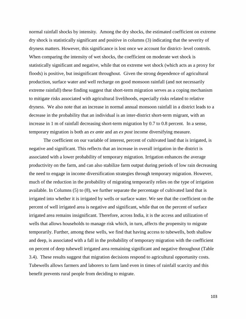
103
normal rainfall shocks by intensity. Among the dry shocks, the estimated coefficient on extreme
dry shock is statistically significant and positive in columns (3) indicating that the severity of
dryness matters. However, this significance is lost once we account for district- level controls.
When comparing the intensity of wet shocks, the coefficient on moderate wet shock is
statistically significant and negative, while that on extreme wet shock (which acts as a proxy for
floods) is positive, but insignificant throughout. Given the strong dependence of agricultural
production, surface water and well recharge on good monsoon rainfall (and not necessarily
extreme rainfall) these finding suggest that short-term migration serves as a coping mechanism
to mitigate risks associated with agricultural livelihoods, especially risks related to relative
dryness. We also note that an increase in normal annual monsoon rainfall in a district leads to a
decrease in the probability that an individual is an inter-district short-term migrant, with an
increase in 1 m of rainfall decreasing short-term migration by 0.7 to 0.8 percent. In a sense,
temporary migration is both an ex ante and an ex post income diversifying measure.
The coefficient on our variable of interest, percent of cultivated land that is irrigated, is
negative and significant. This reflects that an increase in overall irrigation in the district is
associated with a lower probability of temporary migration. Irrigation enhances the average
productivity on the farm, and can also stabilize farm output during periods of low rain decreasing
the need to engage in income diversification strategies through temporary migration. However,
much of the reduction in the probability of migrating temporarily relies on the type of irrigation
available. In Columns (5) to (8), we further separate the percentage of cultivated land that is
irrigated into whether it is irrigated by wells or surface water. We see that the coefficient on the
percent of well irrigated area is negative and significant, while that on the percent of surface
irrigated area remains insignificant. Therefore, across India, it is the access and utilization of
wells that allows households to manage risk which, in turn, affects the propensity to migrate
temporarily. Further, among these wells, we find that having access to tubewells, both shallow
and deep, is associated with a fall in the probability of temporary migration with the coefficient
on percent of deep tubewell irrigated area remaining significant and negative throughout (Table
3.4). These results suggest that migration decisions respond to agricultural opportunity costs.
Tubewells allows farmers and laborers to farm land even in times of rainfall scarcity and this
benefit prevents rural people from deciding to migrate.

104
3.4.2 Impact of Groundwater Levels and Electricity
Given that tubewell use is linked to falling groundwater levels, we assess the impact of
groundwater levels (𝐺𝑊𝐿) on migration decisions and the extent to which this relationship is
mediated through electricity supply (𝐸𝑙𝑒𝑐). We estimate the following:
𝑀𝑖ℎ𝑑 = 𝛽1𝐺𝐷𝐷𝑑 + 𝛽2𝑃𝑑
+ 𝛽3(𝑃𝑑,2006 − 𝑃𝑑 ) (4)
+ 𝛽4𝐺𝑊𝐿 + 𝛽5𝐸𝑙𝑒𝑐 + 𝛽6𝐺𝑊𝐿 ∗ 𝐸𝑙𝑒𝑐
+𝛿1𝑍𝑑 + 𝛿2𝐺𝑖ℎ𝑑 + 𝛿3𝐾ℎ𝑑 + 𝜂𝑡 + 𝜇𝑠 + 𝜖𝑖ℎ𝑑
As explained in Section 3.3.5, we divide districts into those where depths to water table have
consistently been more or less than eight meters over the five years of data available from the
Central Groundwater Board of India. Districts in the former (latter) category are colored as red
(grey) in Figure 3.5. and denoted as D_red region. Areas in white indicate regions that have seen
jumps in groundwater levels above and below eight meters. Therefore, for analysis purposes, we
only compare migration outcomes in the red versus the grey regions. If the red regions have
adapted or invested in technology that allows them to access the scarce water from greater depths,
we would expect the coefficient on D_red region to be negative, meaning that there is a lower
likelihood of inter-district short-term migration from these regions. On the other hand, if the red
regions represent areas that are unable to access the scarce water, then short-term migration from
these areas provide a way to overcome the risk of falling groundwater levels. In this case, the
coefficient on D_red region would be positive. The results are reported in Table 3.5.
The estimates in column (1) show that the coefficient on a continuous measure of the
depth to groundwater is significant and negative so that we fail to reject the hypothesis that there
is relatively less short-term migration in areas with deeper groundwater levels. In column (2),
the coefficient on D_red region is statistically significant and negative, providing further support
for the hypothesis. As discussed in Section 3.3.5, the ability to access scarce water from greater
depths is dependent on having access to electrical pumps that facilitate groundwater extraction.
In columns (3) and (4), we categorize districts based on whether the fraction of villages receiving
electricity supply for agricultural purposes in a particular district is higher than the average for
the country, and interact the indicator for the category with the two measures for groundwater
depth. The coefficient on the continuous measure of depth to groundwater and D_red region is

105
now statistically insignificant. However, the coefficient on the interaction term is significant and
negative at one percent. Therefore, the likelihood of short-term migration falls in districts with
deeper groundwater levels as long as they also have greater electrification.
From column (5), we see that the coefficient on the fraction of villages receiving
electricity supply for agricultural purposes is significant and negative, implying that, in general,
there is a lower chance of individuals migrating from districts with greater electrification. This
effect is strengthened for districts that lie in the red regions, since the coefficient on the
interaction of electrification and D_red region in column (6) is significant and negative.
Therefore, while the net effect of electrification is to lower the degree of short-term migration,
having better access to the benefits of groundwater as a result of higher electricity provision
lowers the chances of short-term migration and increases the agricultural focus of households
even further.
In column (7), we include both D_red region and electrification as predictors. The
results show that with the two regressors the coefficient on fraction of villages electrified
remains strong and negative, while the coefficient on D_red region decreases, and becomes
insignificant. The coefficient on the interaction term too becomes insignificant. Since electricity
supply can have a wide range of spillover effects on the village economy, these results only
suggest that a portion of the groundwater level effect on migration decisions may be attributed to
the higher electrification seen in the red regions relative to the grey regions. Similar results are
found on using nighttime lights as a measure of electrification in Table 3.6.
To further demonstrate that electricity access within a district creates conditions that
enable rural people to mitigate risks associated with agricultural livelihoods, we replicate our
modeling exercise for intra-district short term migration decisions in column (8) of Table 3.5. If
rural people are living in a district that has more access to electricity, we would expect to see
more intra-district short-term migration in these districts. Results show that an increase in
electrification within the district does increase the probability of being an intra-district short-term
migrant; the coefficient is significant at the ten percent level.
3.4.4 Seasonal, Demographic and Household Characteristics:
We plot the coefficients on seasonal, household and individual characteristics in Figures
3.6 and 3.7. The coefficient on quarters of the survey corresponding to the dry season is positive
and significant implying that there are higher chances of short-term migration in the dry season

106
relative to the wet season, when irrigation is a binding constraint on agriculture. This further
confirms that temporary migration is primarily a risk-reducing, and income smoothing livelihood
strategy in rural India. In contrast to examples of labor migration being positively selective for
higher socioeconomic status90
, short-term migration in India is negatively selective for
socioeconomic status and human capital. The probability of short-term migration decreases
across consumption classes such that an increase in MPCE or household income significantly
decreases the probability that a household member is a migrant. Individuals that are employed as
casual agricultural labor, non- agricultural workers, or are unemployed are more likely to be
short-term migrants, than those who are cultivators or self-employed in agriculture. In contrast
to permanent migration, the results show that individuals that are illiterate and with primary
education are significantly more likely to migrate than those with higher levels of education.91
Given these facts, the labor market returns of seasonal migration are not high (Chandrasekhar et
al., 2014). For instance, over 35 percent of the short-term migrants work in the construction
sector and 38 percent continue to work in the primary sector in jobs that are not remunerative.
A larger household size significantly increases the chance that one of the members’ is a
short-term migrant. Households with more members may have surplus labor, and hence activities
can be diversified between members, with some tending to the fields and others migrating.
Figure 3.8 shows the fraction of people of each age who migrated temporarily. The figure shows
the fitted values from local polynomial regressions of a dummy variable that is equal to one if
the individual is a short-term migrant during the time of the survey. The results are presented
separately for males and females. The probability of migrating increases sharply between the
ages of 15 and 30, and strikingly more for males than females. Both men and women migrate
temporarily but a relatively lesser proportion of women are likely to be short-term migrants.92
This is reflected in the estimated coefficients for age, and sex seen in Figure 3.8. Probability of
90
Durand and Massey (1992)’s review of the literature on migration from Mexico to the United States shows that
labor markets in receiving areas select for skilled workers and that the poorest Mexicans are unable to pay the costs
of migration. The NSS survey shows that in India, more educated Indians are more likely to migrate permanently
than temporarily. 91
Using NSS data we find that among the short-term migrants, 40 percent are illiterate, and 71 percent have low
levels of education (were illiterate, did not complete primary school or only completed primary school). 92
Females comprise the largest portion of permanent migrants in India on account of marriage. On the other hand,
the relatively lower short-term mobility of rural women in India can be ascribed to limitations in adjusting their
labor supply due to burdens of childcare, housework, and lack of non-farm work opportunities closer to the village.
In addition cultural norms about women traveling alone, or differential returns from migration might also result in
lower migration. This, in turn, is leading to the feminization of agriculture as the role of women on the farm has
been increasing over the years (Mahajan, 2014; Tumbe, 2014).

107
being a short-term migrant tends to be lower in households that have very large or negligible
amounts of land relative to those with some amount of land. Since land holdings determine
agricultural income, households with some landholding tend to supplement their income through
short-term migration (Chandrasekhar et al., 2014). Certain economically and socially
disadvantaged groups like the SCs and STs are more likely to be short-term migrants93
but the
coefficients are insignificant. Relative to being a Hindu, being a Muslim94
increases the chances
of short-term migration but the effect is also not significant.
Although none of these coefficients are themselves surprising, including these controls
helps verify that these demographic and household factors are not driving the results.
3.5 Robustness Checks
We perform a number of robustness checks. The first check involves using non-linear
models to estimate equations (12) and (13). We estimate a probit model in Table 3.7 and 3.8, and
find that the probit and LPM estimates are close to each other.
The second check explicitly accounts for additional controls for the largest rural workfare
employment program in India. Recent literature provides evidence for a decrease in short-term
migration in rural India as a result of participation in the National Rural Employment Guarantee
Scheme (NREGS) (Imbert and Papp, 2016). In 2006, the Government of India launched the
largest rural workfare program called the NREGS under which every rural household is
guaranteed 100 days of unskilled wage employment at the state minimum wage (Ravi et al.,
2014). It was gradually introduced throughout the country in three phases, starting with 200 of
the poorest districts in February 2006. Later it was extended to 130 districts in April 2007, and to
the rest of rural India in April 2008. Therefore, the NREGS was already in implementation in
330 ‘early’ districts during the first three quarters of the NSS 2007-08 survey from July 2007 to
March 2008 (Imbert and Papp, 2016). During the last quarter of the survey from April 2008 to
June 2008, the NREGS was rolled out to all districts. Our main analysis accounts for the
presence of NREGS since we include all four quarters in our analysis, and control for worker
93
STs have the highest level of poverty in rural areas. 47.4 percent of STs and 42.3 percent of SCs were living
below the poverty line in 2009-10 in rural India (Government of India, 2008). A study by Mosse et al. (2005) based
on a survey in 1996-97 of 42 tribal ‘bhil’ villages found that about 65 percent of the households had temporary
migrants engaging in casual urban construction work. 94
A significant portion of Muslims in India continue to remain below the poverty (33 percent) as per estimates from
2004-05 (Government of India, 2012).

108
employment in public works. Therefore, our estimates for the impact of irrigation and water
access on short-term migration are not confounded due to the absence of controls for NREGS.
Moreover, our analysis does not claim that access to water and irrigation alone decreases
short-term migration, but that in addition to work fare programs, the types of irrigation
infrastructure that are prevalent, and the nature of groundwater development also plays a
fundamental role in influencing short-term migration decisions.
In order to provide further evidence that our estimates are robust to controlling for
NREGS, we include an indicator variable for the ‘early’ districts that had the program before the
nationwide roll-out to all districts in April 2008, and also simultaneously restrict our sample to
observations in the first three quarters of the survey year (July 2007 to March 2008). In this way
we are comparing districts that had the program to those that didn’t. Results are presented in
Tables 3.9a and 3.9b. The estimates in the odd columns remain robust to the exclusion of the last
quarter, and ‘early’ district controls. Further, to account for the uneven implementation of the
NREGS across districts, we add additional controls for seven ‘star’ states: Andhra Pradesh,
Chhattisgarh, Himachal Pradesh, Madhya Pradesh, Rajasthan, Uttarkhand and Tamil Nadu.
These seven states accounted for most of the NREGS employment provision, and therefore
‘early’ districts that fell in these states are likely to have had more employment under the
NREGS (Imbert and Papp, 2016).95
The even columns add an interaction between early districts
and star states, in addition to controlling for early districts. We find that the results remain robust
to these additional controls. Therefore, our estimates are not confounded due to the absence of
sufficient controls for the NREGS.96
The third check models migration decisions at the household level. Traditionally labor
allocation decisions in developing countries have been modeled under the New Economics of
Labor Migration (NELM) framework where a migration decision is modeled as a result of a
household decision making process as opposed to an individual one ( Stark and Bloom, 1985).
To test if our results are sensitive to this type of decision making we estimate equations (12) and
95
The cross-state differences in NREGA provision does not reflect underlying demand for the NREGS, since states
like Bihar or Uttar Pradesh, which have a large population of rural poor provided little NREGA employment (Imbert
and Papp, 2016) 96
Since a portion of the work under the NREGS involves improvements to public water infrastructure, a full
understanding of the interactions between labor mobility and water availability that could change due to NREGS,
and, thus, impact crop choice, agricultural output and productivity is beyond the scope of this study and remains an
important avenue of future research.

109
(13) at the household level, where the dependent variable is the number of household members
who are short-term migrants. We continue to control for household size. We employ a pseudo
maximum likelihood poisson (PPML) estimator as implemented by Silva and Tenreyro (2006) to
account for the count nature of the variable and the large number of zeros.97
This estimator does
not assume equi-dispersion, and is optimal as long as the conditional variance is proportional
(though not necessarily equal) to the conditional mean; hence over-dispersion is not an issue.
Furthermore, the estimator will still be consistent in the case where the conditional variance is
not proportional to the conditional mean. The results in Tables 3.10a and 3.10b are qualitatively
similar to the main results.
The fourth check uses nighttime lights data from other years. Unlike traditional survey
based data or Census records, satellite images are automatically recorded and provide an
unbiased, consistent and objective measure that is unaffected by biases in reporting or poor
measurements. For instance, the Indian government adopted a new definition of electrification in
2004, a year before the launch of the Rajiv Gandhi Grameen Vidyutikaran Yojana (RGGVY),
India’s flagship rural electrification programme in 2005, so that the reported fraction of villages
electrified after 2004 substantially increased. To circumvent concerns that the 2001 Census and
2001 nighttime light data might not capture substantial increases in electrification that followed
in subsequent years in India, we also use nighttime light data from 2006. Studies on India have
found that majority of the variation in light output is cross-sectional, while about 20% of the
variance is observed over time (Min, 2011), so that a single year of nighttime light output data
credibly reflect most of the spatial variation we would expect to see across time.98
In Table 3.11,
we corroborate that our results using nighttime lights data for the year 2006 are similar to our
main results.
3.6 Conclusion
Using nationally representative household -level data, this paper sheds light on the role
that irrigation water access and use might play in affecting adaptation to increased risks of water
scarcity in rural India. Adaptation to environmental stress, especially water scarcity, can take
97
For recent applications, see Burgess et al. (2011), Fetzer (2014) and Colmer (2013). 98
In fact, there could be potential issues when using only time-series variation in nightlights data, since satellite
sensors degrade over time, and there is no on-board calibration of the sensors. Other economics papers have adjusted
for this by using satellite or year fixed effects. Our empirical model relies on cross-sectional variation allaying this
concern.
110
many forms. Therefore, it is crucial to consider how these might interact within a rural economy
when designing and evaluating adaptation and related development policies going forward. In
this paper, we focus on irrigation and short-term migration as two important levers of adaptation.
Our results indicate that water availability and access have an economically significant
impact on rural labor mobility. Higher electricity provision that facilitates groundwater
extraction from greater depths increases the agricultural opportunity cost of rural households and
reduces the degree of short-term migration of its members’. We find that infrastructure that
improves access to water, such as tubewell irrigation, allow individuals to specialize in
agricultural related activities, thereby reducing the likelihood of short-term migration. Irrigation
can, therefore, serve as an alternative to short-term migration as a risk mitigation strategy. From
a policy perceptive, shutting down access to groundwater, in response to rapid depletion will
have significant effects on temporary labor mobility.
However as reserves begin to deplete, new forms of migration might emerge. For
instance, if irrigation enables farm households to improve their agricultural productivity and
household income, and break the income constraint, then it could encourage male members to
switch from temporary migration to more permanent migration. Irrigation access, therefore,
might reduce certain types of migration, but over time, also encourage other type of migration
due to household diversification strategies. Because of data limitations and the cross-sectional
nature of our analysis, we are unable to shed light on these dynamic effects and additional
research will be needed to investigate the interplay of irrigation and temporary migration with
other types of migration, such as remittance -based migration, over a longer time horizon.

111
References
Anderson, S. (2011) Caste as an Impediment to Trade, American Economic Journal: Applied
Economics, 3, 239-263.
Angrist, J. D. (2001) Estimation of Limited Dependent Variable Models with Dummy
Endogenous Regressors: Simple Strategies for Empirical Practice, Journal of Business &
Economic Statistics, 19, 2–16
Badiani, R., K. K. Jessoe, and S. Plant (2012) Development and the Environment: The
Implications of Agricultural Electricity Subsidies in India, The Journal of Environment &
Development, 1070496512442507.
Badiani, R. and A. Safir (2010) Coping with aggregate shocks: Temporary migration and other
labor responses to climatic shocks in rural India, World Bank Mimeo.
Banerjee, A. V. and E. Duflo (2007) The economic lives of the poor, The Journal of Economic
Perspectives, 21, 141.
Basu, D. N., and S.P. Kashyap (1992) Rural Non-agricultural Employment in India: Role of
development process and rural-urban employment linkages, Economic and Political Weekly,
A178-A189.
Bleakley, H. and J. Lin (2012) Portage and Path Dependence, The Quarterly Journal of
Economics, 127(2), 587–644.
de Brauw, A and T. Harigaya (2007) Seasonal Migration and Improving Living Standards in
Vietnam, American Journal of Agricultural Economic, 89(2), 430-447.
Breman, J. (1996) Footloose Labour: Working in India’s Informal Economy, Cambridge
University Press.
Brown, O. (2008) Migration and Climate Change, United Nations Publications.
Brown, L. (2012) World on the edge: how to prevent environmental and economic collapse,
Routledge.
Bryan, G, S. Chowdhury, and A. M. Mobarak (2013) Seasonal Migration and Risk Aversion,
Working Paper
Burgess, R., M. Hansen, B. A. Olken, P. Potapov, and S. Sieber (2011) The political economy of
deforestation in the tropics, Working Paper, National Bureau of Economic Research.

112
Chand, T. R. K, et al. (2009) Spatial characterization of electrical power consumption patterns
over India using temporal DMSP–OLS nighttime satellite data, International Journal of Remote
Sensing, 30(3), 647–661.
Chandrasekhar, S., M. Das, and A. Sharma (2014) Short-term migration and consumption
expenditure of households in rural India, Working Paper, Indira Gandhi Institute of Development
Research, Mumbai, India.
Chopra, K. and S. Gulati (2001) Migration, common property resources and environmental
degradation: interlinkages in India's arid and semi-arid regions, Sage Publications.
Coffey, D., J. Papp, and D. Spears (2014) Short-Term Labor Migration from Rural North India:
Evidence from New Survey Data, Population Research and Policy Review, 1-20.
Colmer, J. (2013) Climate Variability, Child Labour and Schooling: Evidence on the Intensive
and Extensive Margin, Nota di Lavoro, Fondazione Eni Enrico Mattei.
Dallmann, I. and K. Millock (2013) Climate Variability and Internal Migration: A Test on Indian
Inter-State Migration, Paris School of Economics, Working Paper.
Deshingkar, P. and J. Farrington (2009) A Framework for Understanding Circular Migration,
Oxford University Press.
Dubash, N. K. (2002) Tubewell capitalism: groundwater development and agrarian change in
Gujarat. Oxford University Press, New Delhi
Durand, J. and D. Massey (1992) Mexican migration to the United States: A critical review,
Latin American Research Review, 27 (2), 3-42.
Elvidge, C. et al. 1997 Relation between satellite observed visible-near infrared emissions,
population, economic activity, and power consumption, International Journal of Remote Sensing,
18(6):1373–1379.
Feng, S., A. B. Krueger, and M. Oppenheimer (2010) Linkages among climate change, crop
yields and Mexico-US cross-border migration, Proceedings of the National Academy of Sciences,
107, 14257-14262.
Fetzer, T. (2014) Can workfare programs moderate violence? Evidence from India, Job Market
Paper.
Fishman, R., M. Jain and A. Kishore (2015) When Water Runs Out: Scarcity, Adaptation and
Migration in Gujarat, International Growth Center Working Paper

113
Gandhi, V.P. and Namboodiri, N.V. (2009) Groundwater irrigation in India: Gains, costs, and
risks. Ahmedabad, India: Indian Institute of Management
Government of India (2012) Press Note on Poverty Estimates, 2009-10, Planning Commission,
Government of India
Government of India (2008) Annual Report 2007-08, Ministry of Rural Development,
Government of India Available at http://www.rural.nic.in/sites/downloads/annualreport/
anualreport0708_eng.pdf
Gupta, A. K., D. M. Anderson, D. N. Pandey, and A. K. Singhvi (2006) Adaptation and human
migration, and evidence of agriculture coincident with changes in the Indian summer monsoon
during the Holocene, Current Science, 90, 1082-1090.
Haberfeld, Y., R. Menaria, B. B. Sahoo, and R. Vyas (1999) Seasonal migration of rural labor in
India, Population Research and Policy Review, 18, 471-487.
Harris, J. and M. P. Todaro (1970) Migration, unemployment and development: A two sector
analysis, American Economic Review 60 (1), 126-142.
Henderson, J. V., A. Storeygard, and D. N. Weil (2012) Measuring Economic Growth from
Outer Space, American Economic Review 102(2), 994–1028
Horrace, W. C., and R.L. Oaxaca (2006) Results on the bias and inconsistency of ordinary least
squares for the linear probability model, Economic Letters, 321-327.
Hornbeck, R. (2012) The Enduring Impact of the American Dust Bowl: Short-and Long-Run
Adjustments to Environmental Catastrophe, American Economic Review, 102, 1477-1507.
Hornbeck, R. and S. Naidu (2014) When the Levee Breaks: Black Migration and Economic
Development in the American South, American Economic Review, 104, 963-90.
Imbert, C. and J. Papp (2016) Short-term Migration and Rural Workfare Programs: Evidence
from India, Working Paper.
Ito, T., and T. Kurosaki (2009) Weather Risk, Wages in Kind, and the Off‐Farm Labor Supply of
Agricultural Households in a Developing Country, American Journal of Agricultural Economics,
697‐710.
Jayachandran, S. (2006) Selling labor low: Wage responses to productivity shocks in developing
countries, Journal of Political Economy, 114, 538-575.
Jessoe, K. and R. Badiani (2015) The Impact of Electricity Subsidies on Groundwater Extraction
and Agricultural Production. Working Paper.

114
Keshri, K. and R. Bhagat (2012) Temporary and seasonal migration: Regional pattern,
characteristics and associated factors, Economic and Political Weekly, 47, 81-88.
Klaassen, F. and J. Magnus (2001) Are Points in Tennis Independent and Identically Distributed?
Evidence From a Dynamic Binary Panel Data Model, Journal of the American Statistical
Association, 500- 509
Klaiber, H. A. (2014) Migration and household adaptation to climate: A review of empirical
research, Energy Economics, 46, 539-547.
Kochar, A. (1999) Smoothing consumption by smoothing income: hours-of-work responses to
idiosyncratic agricultural shocks in rural India, Review of Economics and Statistics, 81, 50-61.
Krishnan, R., T. P. Sabin, R. Vellore, et al. (2015) Deciphering the desiccation trend of the South
Asian monsoon hydroclimate in a warming world, Clim. Dynam. 1-21
Kumar, H., and R. Somanathan (2009) Mapping Indian districts across census years, 1971-
2001, Centre for Development Economics Working Paper, 176.
Kurosaki, T., and M. Fafchamps (2002) Insurance Market Efficiency and Crop Choices in
Pakistan, Journal of Development Economics, 67(2):419–53.
Lanjouw, P. and A. Shariff (2004) Rural Non-Farm Employment in India: Access, Incomes and
Poverty Impact, Economic and Political Weekly, 39 (40), 4429-4446.
Macours, K. and R. Vakis (2010) Seasonal Migration and Early Childhood Development, World
Development, 38(6), 857-869.
Mahajan, K (2014) Blame it on the Rain? : Gender differentiated impacts of drought on
agricultural wage and work in India, United Nations Development Programme Publication,
Regional Bureau for Asia and the Pacific
Marchiori, L., J.-F. Maystadt, and I. Schumacher (2012) The impact of weather anomalies on
migration in sub-Saharan Africa," Journal of Environmental Economics and Management, 63,
355-374.
Min, B. (2011) Electrifying the Poor: Distributing Power in India, Manuscript.
Min, B. et al. (2013) Detection of rural electrification in Africa using DMSP-OLS night lights
imagery, International Journal of Remote Sensing, 34 (22), 8118–8141
Min, B. and K. M. Gaba (2014) Tracking Electrification in Vietnam Using Nighttime Lights,
Remote Sensing, 6(10), 9511–9529.

115
Moench, M. (2002) Water and the potential for social instability: livelihoods, migration and the
building of society, In Natural Resources Forum, vol. 26, 195-204, Wiley Online Library
Morten, M. (2014) Temporary migration and endogenous risk sharing in village India, Working
Paper.
Mosse, D., S. Gupta, M. Mehta, V. Shah, J. f. Rees, and K. P. Team (2002) Brokered livelihoods:
debt, labour migration and development in tribal western India, Journal of Development Studies,
38, 59-88.
Mukherji, A., B. Das, N. Majumdar, N. C. Nayak, R. R. Sethi, and B. R. Sharma (2009)
Metering of agricultural power supply in West Bengal, India: Who gains and who loses? Energy
Policy 37, 5530-5539.
Mukherji, A., S. Rawat, and T. Shah (2013) Major Insights from India’s Minor Irrigation
Censuses: 1986-87 to 2006-07, Economic & Political Weekly, 48(26), 115-124.
Mullahy, J. (1990) Weighted least squares estimation of the linear probability model, revisited,
Economics Letters, 35-41.
Mundial, B. (2009) World Development Report 2009: Reshaping Economic Geography, World
Bank, Washington D.C.
Munshi, K. and M. Rosenzweig (2009) Why is mobility in India so low? Social insurance,
inequality, and growth, Working Paper, National Bureau of Economic Research. .
Nair, K. N. and S. Chattopadhyay (2005) Water resources of Kerala. Issues and case studies,
Center for Development Studies: Thiruvananthapuram.
National Sample Survey Organization (2010) Employment and Unemployment situation in India
2007-08 NSS 64th Round July 2007 to June 2008, Technical report, Ministry of Statistics and
Programme Implementation, Government of India.
Parry, M. L, O.F. Canziani, J. P. Palutikof, P. J van der Linden, and C. E Hanson (2007) IPCC
2007: Climate Change 2007: Impacts, adaptation and vulnerability, Contribution of Working
Group II to the fourth assessment report of the Intergovernmental Panel on Climate Change.
Prakash, A. (2005) The dark zone: Groundwater irrigation, politics and social power in North
Gujarat, vol. 7, Orient Blackswan.
Rappaport, J. (2007) Moving to nice weather, Regional Science and Urban Economics, 37, 375-
398.
116
Ravi, S., M. Kapoor, and R. Ahluwalia (2014) The Impact of NREGS on Urbanization in India,
Working Paper.
Reardon, T., J. Berdegué, C.B. Barrett, and K. Stamoulis (2006) Household Income
Diversification into Rural Nonfarm Activities, In S. Haggblade, P. Hazell, & T. Reardon,
Transforming the Rural Nonfarm Economy. Baltimore: Johns Hopkins University Press.
Rose, E. (2001) Ex Ante and Ex Post Labour Supply Responses to Risk in a Low Income Area,
Journal of Development Economics, 64(2), 371-388.
Rosenzweig, M. R. and H. P. Binswanger (1993) Wealth, Weather Risk and the Composition and
Profitability of Agricultural Investments, Economic Journal, 103, 56-78.
Rosenzweig, M. R. and O. Stark (1989) Consumption smoothing, migration, and marriage:
Evidence from rural India, The Journal of Political Economy, 905-926.
Sekhri, S. (2011) Public provision and protection of natural resources: Groundwater irrigation in
rural India, American Economic Journal: Applied Economics, 29-55.
Sekhri, S. (2013) Missing Water: Agricultural Stress and Adaptation Strategies in response to
Groundwater Depletion among Farmers in India, Working Paper
Singh, D., M. Tsiang, B. Rajaratnam, and N. S. Diffenbaugh (2014) Observed changes in
extreme wet and dry spells during the South Asian summer monsoon season, Nature Climate
Change, 4(6), 456-461.
Sigman, H. and S. Olmstead (2016) Droughts, Dams, and Economic Activity, Working Paper.
Silva, J. S. and S. Tenreyro (2006) The log of gravity, The Review of Economics and
Statistics, 88(4), 641-658.
Sjaastad, L. A. (1962) The costs and returns of human migration, The Journal of Political
Economy, 70(5), 80-93.
Stark, O. and D. E. Bloom (1985) The new economics of labor migration, American Economic
Review, 75(2), 173-178.
Stark, O. and D. Levhari (1982) On migration and risk in LDCs, Economic development and
Cultural Change, 31(1), 191-196.
Storeygard, A. (2013) Farther on down the road: transport costs, trade and urban growth in Sub-
Saharan Africa, Policy Research Working Paper Series 6444, The World Bank
Taraz, V. (2014) Adaptation to Climate Change: Historical Evidence from the Indian Monsoon,
Yale University, Job Market Paper.

117
Todaro, M. P. (1969) A model of labor migration and urban unemployment in less developed
countries, American Economic Review, 59(1), 138-148.
Topalova, P. (2010) Factor immobility and regional impacts of trade liberalization: Evidence
on poverty from India, American Economic Journal: Applied Economics, 2(4), 1-41.
Tumbe, C. (2014) The Great Indian Migration Wave, 1870-2010: Persistence & Consequences,
Economic Growth Center, Working Paper.
Turner, A.G., and H.Annamalai (2012) Climate change and the South Asian summer monsoon,
nat. Clim.Change, 2(8), 597-595.
Udry, C. (1994) Risk and insurance in a rural credit market: An empirical investigation in
northern Nigeria, The Review of Economic Studies, 61, 495-526.
Viswanathan, B. and K.S. Kavi Kumar (2015) Weather, agriculture and rural migration:
evidence from state and district level migration in India. Environment and Development
Economics, 20, 469-492.
Vorosmarty, C. J., P. Green, J. Salisbury, and R.B Lammers (2000) Global water resources:
vulnerability from climate change and population growth. Science, 289, 284-288.
Warner, K. (2010) Global environmental change and migration: Governance challenges, Global
Environmental Change, 20, 402-413.
Wooldridge, J.M (2002) Econometric Analysis of Cross Section and Panel Data, The MIT Press.
World Bank (2016) High and Dry: Climate Change, Water, and the Economy, World Bank,
Washington D.C.

118
% Rural Households with Short-term Migrants
68 11 0
Figures
Fig. 3.1: Short-term migration
Notes: The maps shows the percent of rural households with short-term migrants for each district; state
boundaries are in black. Nationally, around 7% of rural households have short-term migrants. Data is from
the NSS 2007-08 survey.

119
Fig. 3.2: Spatial distribution of electricity provision
Notes: The panels show the geographic distribution of electrification using 2001 Census data (A) and 2001
nighttime lights data (B) . Gradations of black indicate lower electrification, and gradations of white indicate higher
electrification. Panel A maps the fraction of villages electrified in each district; state boundaries are in black. Panel
B maps the pixel values for luminosity with 0 indicating no luminosity, and 63 indicating highest luminosity.
Measure of luminosity
B A
Fraction of villages electrified

120
30
35
40
45
50
55
60
65
1993-94 2000-01
% o
f vi
llage
s
groundwater depth < 10m
groundwater depth > 10 m
0
10
20
30
40
50
60
70
80
1986-87 1993-94 2000-01 2006-07
% o
f gr
ou
nd
wat
er
stru
ctu
res
Deep tube wells Shallow tube wells Dug wells
Fig. 3.3: Percentage of villages according to depth to groundwater
Notes: Groundwater depth indicates depth to water table in meters below ground level
(mbgl). Data is from the Minor Irrigation Census 1993-94 and 2000-01.
Fig. 3.4: Percentage of groundwater structures
Notes: Data is from the Minor Irrigation Census 1986-87, 1993-94, 2000-01 and 2006-07.
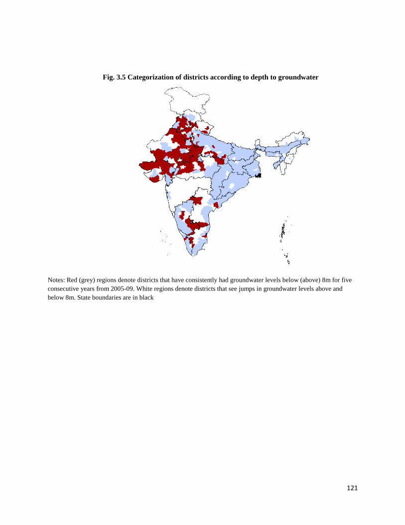
121
Fig. 3.5 Categorization of districts according to depth to groundwater
Notes: Red (grey) regions denote districts that have consistently had groundwater levels below (above) 8m for five
consecutive years from 2005-09. White regions denote districts that see jumps in groundwater levels above and
below 8m. State boundaries are in black

122
Fig. 3.6 Coefficient estimates for household and individual characteristics
Notes: Coefficient estimates from results in Column (1) of Table 3.3 with 95% confidence intervals
Fig. 3.7 Coefficient estimates for individual employment status
Notes: Coefficient estimates from results in Column (1) of Table 3.3 with 95% confidence intervals

123
0
.05
.1.1
5
Fra
ctio
n w
ho le
ft a
s s
hort
-te
rm m
igra
nts
0 20 40 60 80Age
Male Female
Fig. 3.8 Short-term migrants by age and sex
Notes: Data is from the NSS 2007-08 survey.

124
Tables
Note: Data from NSS 2007-08 survey. Statistics computed using weights
Table 3.1. Short-term Migrants (STMs)
Rural population 743,596,830
STMs (rural) 12,584,607
Inter-district versus Intra- district STMs
% Inter-district STMs 80.98%
% Intra-district STMs 18.47%
Rural versus Urban
% Inter-district STMs going to rural areas 22.54%
% Inter-district STMs going to urban areas 58.43%
% Intra-district STMs going to rural areas 9.94%
% Intra-district STMs going to urban areas 8.54%
% of STMs in rural areas who have lived in place of
enumeration :
Always (i.e., never migrated from another place)
84% (10,543,568)
Since 0 to > 40 years (i.e., migration from another place between 0 to > 40 years ago)
16% (2,041,039)
Break-up by years
≤ 5 years
( i.e., migrated from another place ≤ 5 years ago)
6.5% (823,246)
6-10 years 2.3% (300,786)
11-20 years 4.2% (535,239)
21-30 years 1.9% (249,229)
31-40 years 0.56% (71,351)
> 40 years 0.18% (23,851)
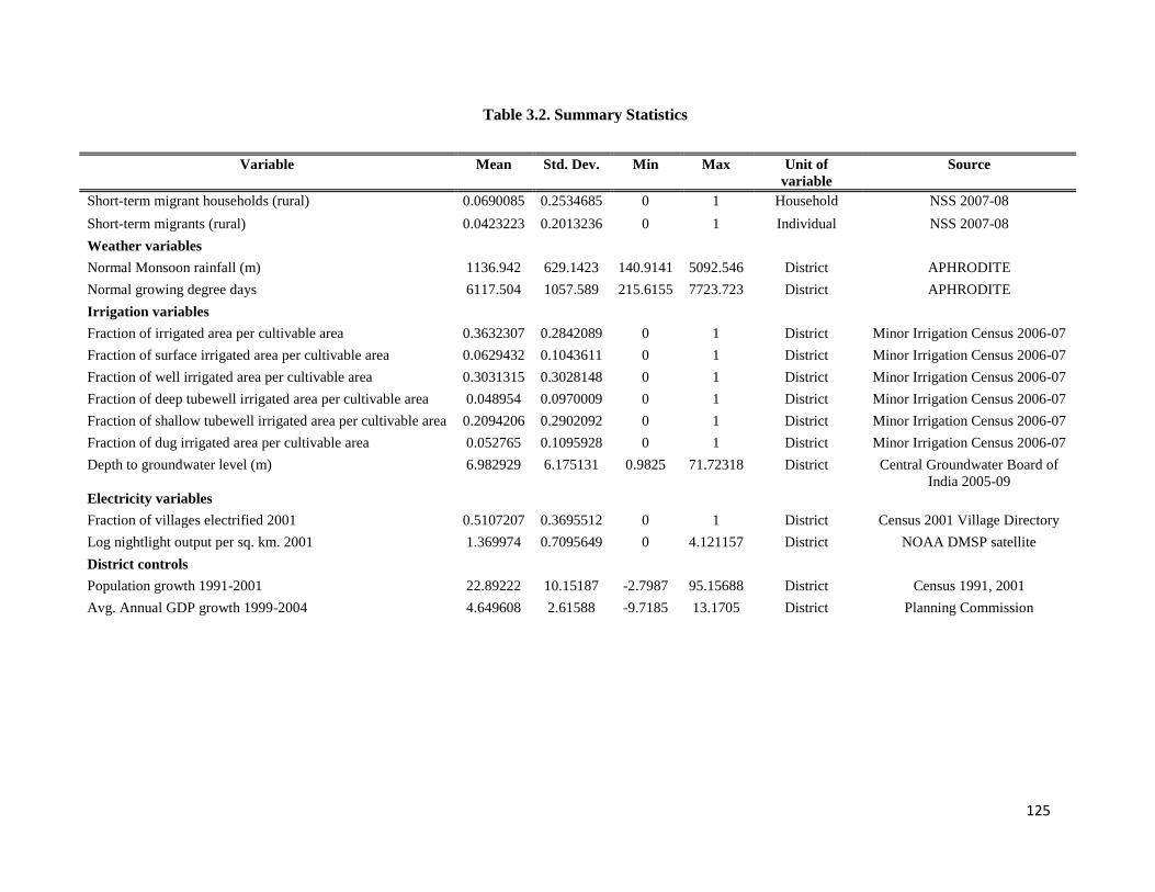
125
Variable Mean Std. Dev. Min Max Unit of
variable
Source
Short-term migrant households (rural) 0.0690085 0.2534685 0 1 Household NSS 2007-08
Short-term migrants (rural) 0.0423223 0.2013236 0 1 Individual NSS 2007-08
Weather variables
Normal Monsoon rainfall (m) 1136.942 629.1423 140.9141 5092.546 District APHRODITE
Normal growing degree days 6117.504 1057.589 215.6155 7723.723 District APHRODITE
Irrigation variables
Fraction of irrigated area per cultivable area 0.3632307 0.2842089 0 1 District Minor Irrigation Census 2006-07
Fraction of surface irrigated area per cultivable area 0.0629432 0.1043611 0 1 District Minor Irrigation Census 2006-07
Fraction of well irrigated area per cultivable area 0.3031315 0.3028148 0 1 District Minor Irrigation Census 2006-07
Fraction of deep tubewell irrigated area per cultivable area 0.048954 0.0970009 0 1 District Minor Irrigation Census 2006-07
Fraction of shallow tubewell irrigated area per cultivable area 0.2094206 0.2902092 0 1 District Minor Irrigation Census 2006-07
Fraction of dug irrigated area per cultivable area 0.052765 0.1095928 0 1 District Minor Irrigation Census 2006-07
Depth to groundwater level (m) 6.982929 6.175131 0.9825 71.72318 District Central Groundwater Board of
India 2005-09
Electricity variables
Fraction of villages electrified 2001 0.5107207 0.3695512 0 1 District Census 2001 Village Directory
Log nightlight output per sq. km. 2001 1.369974 0.7095649 0 4.121157 District NOAA DMSP satellite
District controls
Population growth 1991-2001 22.89222 10.15187 -2.7987 95.15688 District Census 1991, 2001
Avg. Annual GDP growth 1999-2004 4.649608 2.61588 -9.7185 13.1705 District Planning Commission
Table 3.2. Summary Statistics

126
Variable Mean Std. Dev. Min Max Unit of
variable
Households and Individual controls
Household size 5.876848 2.734402 1 30 Household
Log monthly per capita expenditure (mpce) 8.112304 0.5370774 3.988984 12.18499 Household
Female 0.4919321 0.4999356 0 1 Individual
Age 34.93839 14.15645 15 65 Individual
Married 0.4678377 0.4989652 0 1 Individual
Land posession
< 1 hectares 0.766111 0.423303 0 1 Household
1-4 hectares 0.21 0.40 0 1 Household
> 4 hectares 0.0278947 0.1646714 0 1 Household
Religion
Hindu 0.78 0.41 0 1 Individual
Muslim 0.11 0.31 0 1 Individual
Christian 0.0690877 0.2536035 0 1 Individual
Others 0.0438734 0.2048138 0 1 Individual
Social Caste
Schedules Caste/ Schedulted Tribe (SC/ST) 0.3623018 0.480666 0 1 Individual
Other Backward Class (OBC) 0.403675 0.4906344 0 1 Individual
Others 0.2340233 0.4233874 0 1 Individual
Education levels
Illiterate 0.392433 0.4882929 0 1 Individual
Primary 0.3404533 0.4738623 0 1 Individual
Middle and Secondary 0.205043 0.4037336 0 1 Individual
Higher Secondary and above 0.0620707 0.2412843 0 1 Individual
Employment Status Before Migrating
Unemployed 0.0136375 0.1159806 0 1 Individual
Casual Agricultural Labor 0.1290418 0.3352467 0 1 Individual
Non-Agricultural Work 0.0980759 0.2974176 0 1 Individual
Cultivator 0.2365446 0.4249609 0 1 Individual
Salaried Work 0.0363116 0.1870645 0 1 Individual
Public Work 0.0041473 0.064266 0 1 Individual
Table 3.2. Summary Statistics (continued)

127
Short-term migrant (inter-district)
Notes: The sample is composed of all individuals aged 15 to 65 interviewed from July 2007 to June 2008. Dependent variable is a binary variable which is equal to 1 if an individual has spent one
to six months away from work during the last year and zero otherwise. Each column presents a separate regression. Standard errors are reported in the parentheses and are clustered by district. All
regressions include sub- round fixed effects, state fixed effects, household and individual controls. District controls include indicators for districts with high population growth between 1991 and
2001 censuses relative to the national average, districts with high average annual GDP growth between 1999 and 2005 relative to the national average. Household controls include log of MPCE,
household size, landholding size. Individual controls include age, gender, education levels, marital status, religion, caste, employment status. + p<0.10 * p<0.05 ** p <0.01 ***p < 0.001.
Table 3.3. Likelihood of short-term migration in response to irrigation
(1) (2) (3) (4) (5) (6) (7) (8)
Normal Annual GDDs (1000 deg days) 0.00427 0.00425 0.00416 0.00412 0.00397 0.00396 0.00383 0.00377
(0.00305) (0.00302) (0.00310) (0.00310) (0.00307) (0.00305) (0.00312) (0.00313)
Normal Monsoon Precip (m) -0.00781+ -0.00743+ -0.00344 -0.00294 -0.00859* -0.00825* -0.00502 -0.00450
(0.00419) (0.00403) (0.00600) (0.00607) (0.00414) (0.00399) (0.00592) (0.00595)
Rainfall shock in 2006 (m) -0.02676* -0.02417* -0.02741* -0.02500*
(0.01208) (0.01214) (0.01205) (0.01213)
Extreme dry shock (m) 0.05755+ 0.05152 0.04870 0.04245
(0.03408) (0.03284) (0.03319) (0.03194)
Moderate dry shock (m) -0.01335 -0.00908 -0.01590 -0.01120
(0.02643) (0.02649) (0.02629) (0.02624)
Moderate wet shock (m) -0.08124* -0.07883* -0.08067* -0.07943*
(0.03745) (0.03979) (0.03718) (0.03945)
Extreme wet shock (m) 0.01076 0.00790 0.01541 0.01254
(0.02397) (0.02370) (0.02400) (0.02379)
% Irrigated area/cultivated area -0.00023* -0.00024* -0.00021* -0.00023*
(0.00011) (0.00011) (0.00011) (0.00011)
% Surface irrigated area/cultivated area 0.00022 0.00023 0.00023 0.00024
(0.00023) (0.00023) (0.00023) (0.00023)
% Well irrigated area/cultivated area -0.00032** -0.00033** -0.00030** -0.00031**
(0.00010) (0.00010) (0.00010) (0.00010)
District controls No Yes No Yes No Yes No Yes
N 213246 213246 213246 213246 213246 213246 213246 213246
R-sq 0.088 0.088 0.088 0.088 0.088 0.088 0.088 0.088

128
Short-term migrant (inter-district)
Notes: The sample is composed of all individuals aged 15 to 65 interviewed from July 2007 to June 2008. Dependent variable is a binary
variable which is equal to 1 if an individual has spent one to six months away from work during the last year and zero otherwise. Each
column presents a separate regression. Standard errors are reported in the parentheses and are clustered by district. All regressions
include sub- round fixed effects, state fixed effects, household and individual controls. District controls include indicators for districts
with high population growth between 1991 and 2001 censuses relative to the national average, districts with high average annual GDP
growth between 1999 and 2005 relative to the national average. Household controls include log of MPCE, household size, landholding
size. Individual controls include age, gender, education levels, marital status, religion, caste, employment status. + p<0.10 * p<0.05 ** p
<0.01 ***p < 0.001.
Table 3.4. Likelihood of short-term migration in response to the type of irrigation
(1) (2) (3)
Normal Annual GDDs (1000 deg days) 0.00431 0.00443 0.00433
(0.00310) (0.00316) (0.00317)
Normal Monsoon Precip (m) -0.00811* -0.00447 -0.00391
(0.00407) (0.00586) (0.00593)
Rainfall shock in 2006 (m) -0.02597*
(0.01221)
Extreme dry shock (m) 0.05940+ 0.05494
(0.03495) (0.03434)
Moderate dry shock (m) -0.01528 -0.01097
(0.02621) (0.02624)
Moderate wet shock (m) -0.09059* -0.09067*
(0.03981) (0.04276)
Extreme wet shock (m) 0.02537 0.02268
(0.02568) (0.02565)
% Surface irrigated area/cultivated area 0.00024 0.00021 0.00022
(0.00022) (0.00021) (0.00022)
% Deep tubewell irrigated area/cultivated area -0.00052** -0.00058** -0.00056**
(0.00019) (0.00019) (0.00019)
% Shallow tubewell irrigated area/cultivated area -0.00021+ -0.00018 -0.00020+
(0.00012) (0.00012) (0.00012)
% Dugwell irrigated area/cultivated area -0.00013 0.00001 -0.00001
(0.00024) (0.00027) (0.00027)
District controls Yes No Yes
N 213064 213064 213064
R-sq 0.088 0.088 0.088

129
Inter-district Intra-district
(1) (2) (3) (4) (5) (6) (7) (8)
Normal Annual GDDs (1000 deg days) 0.00291 0.00223 0.00338 0.00392 0.00489+ 0.00438+ 0.00459+ 0.00063
(0.00461) (0.00265) (0.00450) (0.00264) (0.00252) (0.00253) (0.00262) (0.00107)
Normal Monsoon Precip (m) -0.00755* -0.00745* -0.00784* -0.00929** -0.00956** -0.01067** -0.01073** 0.00002
(0.00351) (0.00348) (0.00348) (0.00337) (0.00323) (0.00330) (0.00331) (0.00142)
Rainfall shock in 2006 (m) -0.02531* -0.02576* -0.02685* -0.02958* -0.02781* -0.02919* -0.02948* 0.00357
(0.01182) (0.01169) (0.01175) (0.01146) (0.01154) (0.01159) (0.01166) (0.00335)
Depth to groundwater 2006 (m) -0.00103** 0.00045
(0.00036) (0.00057)
D_red region -0.01782** -0.01372 -0.00673 0.00231
(0.00638) (0.00984) (0.01356) (0.00343)
Depth to groundwater 2006 (m) x high electricity -0.00169**
(0.00056)
D_red region x high electricity -0.02785**
(0.00999)
% villages with electricity -0.04115** -0.03640** -0.03737** 0.00591+
(0.01393) (0.01379) (0.01445) (0.00330)
D_red region x % village with electricity -0.02032** -0.01260 -0.00490
(0.00767) (0.01706) (0.00481)
N 210043 233852 210043 233852 233852 233852 233852 362794
R-sq 0.088 0.088 0.089 0.088 0.088 0.088 0.088 0.020
Notes: The sample is composed of all individuals aged 15 to 65 interviewed from July 2007 to June 2008. Dependent variable is a binary variable which is equal to 1 if an individual has spent one
to six months away from work during the last year and zero otherwise. Each column presents a separate regression. Standard errors are reported in the parentheses and are clustered by district. All
regressions include sub- round fixed effects, state fixed effects, district, household and individual controls. District controls include indicators for districts with high population growth between
1991 and 2001 censuses relative to the national average, districts with high average annual GDP growth between 1999 and 2005 relative to the national average. Household controls include log of
MPCE, household size, landholding size. Individual controls include age, gender, education levels, marital status, religion, caste, employment status. + p<0.10 * p<0.05 ** p <0.01 ***p < 0.001
Table 3.5. Likelihood of short-term migration in response to groundwater levels and electricity provision

130
Notes: The sample is composed of all individuals aged 15 to 65 interviewed from July 2007 to June 2008. Dependent variable is a
binary variable which is equal to 1 if an individual has spent one to six months away from work during the last year and zero
otherwise. Each column presents a separate regression. Standard errors are reported in the parentheses and are clustered by district.
All regressions include sub- round fixed effects, state fixed effects, district, household and individual controls. District controls
include indicators for districts with high population growth between 1991 and 2001 censuses relative to the national average, districts
with high average annual GDP growth between 1999 and 2005 relative to the national average. Household controls include log of
MPCE, household size, landholding size. Individual controls include age, gender, education levels, marital status, religion, caste,
employment status. + p<0.10 * p<0.05 ** p <0.01 ***p < 0.001
Table 3.6. Likelihood of short-term migration in response to groundwater levels and electricity
provision (Night lights)
Short-term migrant (inter-district)
(1) (2) (3) (4) (5)
Normal Annual GDDs (1000 deg days) 0.00291 0.00223 0.00898*** 0.00839** 0.00887**
(0.00461) (0.00265) (0.00262) (0.00264) (0.00272)
Normal Monsoon Precip (m) -0.00755* -0.00745* -0.00775* -0.00852* -0.00872*
(0.00351) (0.00348) (0.00334) (0.00337) (0.00339)
Rainfall shock in 2006 (m) -0.02531* -0.02576* -0.00975 -0.01223 -0.01200
(0.01182) (0.01169) (0.01158) (0.01191) (0.01188)
Depth to groundwater 2006 (m) -0.00103**
(0.00036)
D_red region -0.01782** -0.01492
(0.00638) (0.01546)
log nightlight output per sq. km. -0.02817*** -0.02599*** -0.02702***
(0.00412) (0.00415) (0.00444)
D_red region x log nightlight output per sq.
km.
-0.00607* 0.00135
(0.00278) (0.00675)
N 210043 233852 233852 233852 233852
R-sq 0.088 0.088 0.090 0.090 0.090

131
Notes: The sample is composed of all individuals aged 15 to 65 interviewed from July 2007 to June 2008. Dependent variable is a
binary variable which is equal to 1 if an individual has spent one to six months away from work during the last year and zero
otherwise. Coefficients are marginal effects estimated at mean values of the data. Standard errors are reported in the parentheses and
clustered by district. All regressions include sub- round fixed effects, state fixed effects, district, household and individual controls as
indicated in Table 3.3. + p<0.10 * p<0.05 ** p <0.01 ***p < 0.001
Table 3.7. Robustness Checks: Likelihood of short-term migration in response to irrigation (Probit)
Short-term migrant (inter-district)
(1) (2) (3) (4) (5) (6)
Normal Annual GDDs (1000 deg days) 0.00250 0.00273 0.00228 0.00246 0.00264 0.00291
(0.00188) (0.00190) (0.00190) (0.00192) (0.00194) (0.00197)
Normal Monsoon Precip (m) -0.00612* -0.00243 -0.00660** -0.00317 -0.00688** -0.00327
(0.00243) (0.00292) (0.00245) (0.00288) (0.00248) (0.00284)
Rainfall shock in 2006 (m) -0.01531* -0.01597* -0.01730**
(0.00624) (0.00621) (0.00626)
Extreme dry shock (m) 0.03326+ 0.02829 0.03173+
(0.01895) (0.01829) (0.01895)
Moderate dry shock (m) -0.00268 -0.00345 -0.00452
(0.00958) (0.00931) (0.00924)
Moderate wet shock (m) -0.04936* -0.05075* -0.05433*
(0.02259) (0.02228) (0.02275)
Extreme wet shock (m) -0.00732 -0.00386 -0.00070
(0.01961) (0.01955) (0.01955)
% Irrigated area/cultivable area -0.00009* -0.00009*
(0.00004) (0.00004)
% Surface irrigated area/cultivable area 0.00010 0.00010 0.00011 0.00010
(0.00009) (0.00009) (0.00008) (0.00008)
% Well irrigated area/cultivable area -0.00013** -0.00012**
(0.00004) (0.00004)
% Deep tubewell irrigated area/cultivable area -0.00032** -0.00033**
(0.00011) (0.00011)
% Shallow tubewell irrigated area/cultivable
area
-0.00005 -0.00005
(0.00004) (0.00004)
% Dugwell irrigated area/cultivable area -0.00006 -0.00003
(0.00011) (0.00011)
N 213048 213048 213048 213048 212866 212866
Log likelihood -32066.554 -32020.94 -32030.609 -31985.602 -32006.169 -31955.674

132
Notes: The sample is composed of all individuals aged 15 to 65 interviewed from July 2007 to June 2008. Dependent variable is a binary variable which is equal to 1 if an individual
has spent one to six months away from work during the last year and zero otherwise. Coefficients are marginal effects estimated at mean values of the data. Standard errors are
reported in the parentheses and clustered by district. All regressions include sub- round fixed effects, state fixed effects, district, household and individual controls as indicated in Table
3.3. + p<0.10 * p<0.05 ** p <0.01 ***p < 0.001
Table 3.8. Robustness Checks: Likelihood of short-term migration in response to groundwater levels and electricity provision (Probit)
Short-term migrant
Inter-district Intra-district
(1) (2) (3) (4) (5) (6) (7) (8)
Normal Annual GDDs (1000 deg days) 0.00145 0.00110 0.00168 0.00076 0.00230 0.00189 0.00188 0.00035
(0.00244) (0.00149) (0.00235) (0.00148) (0.00144) (0.00141) (0.00143) (0.00058)
Normal Monsoon Precip (m) -0.00671** -0.00588** -0.00676** -0.00595** -0.00622*** -0.00689*** -0.00688*** -0.00013
(0.00222) (0.00196) (0.00218) (0.00194) (0.00185) (0.00187) (0.00188) (0.00058)
Rainfall shock in 2006 (m) -0.01613** -0.01500** -0.01672** -0.01474** -0.01443** -0.01517** -0.01514** 0.00098
(0.00604) (0.00541) (0.00586) (0.00534) (0.00524) (0.00515) (0.00515) (0.00133)
Depth to groundwater 2006 (m) -0.00065** 0.00004
(0.00020) (0.00023)
D_red region -0.00702*** 0.00005 0.00067 0.00164
(0.00185) (0.00300) (0.00547) (0.00256)
Depth to groundwater 2006 (m) x high electricity -0.00086***
(0.00023)
D_red region x high electricity -0.01034**
(0.00375)
% villages with electricity -0.01503** -0.01250* -0.01242* 0.00349*
(0.00529) (0.00517) (0.00535) (0.00176)
D_red region x % villages with electricity
-0.01011** -0.01088 -0.00260
(0.00327) (0.00725) (0.00255)
N 209845 233654 209845 233654 233654 233654 233654 362501
Log likelihood -31953.595 -33877.403 -31891.106 -33851.918 -33896.388 -33813.31 -33813.263 -17092.153

133
Notes: The sample is composed of all individuals aged 15 to 65 interviewed from July 2007 to June 2008. Dependent variable is a binary variable which is equal to 1 if an individual has spent one
to six months away from work during the last year and zero otherwise. Standard errors are reported in the parentheses and clustered by district. All regressions include sub- round fixed effects,
state fixed effects, district, household and individual controls as indicated in Table 3.3. Early District is a dummy variable equal to one for districts in which NREGS is implemented. Star is a
dummy variable equal to one for Andhra Pradesh, Himachal Pradesh, Chhattisgarh, Madhya Pradesh, Rajasthan, Tamil Nadu and Uttarakhand. + p<0.10 * p<0.05 ** p <0.01 ***p < 0.001
Table 3.9a. Robustness Checks: NREGS and likelihood of short-term migration in response to irrigation
Short-term migrant (inter-district)
(1) (2) (3) (4) (5) (6)
Normal Annual GDDs (1000 deg days) 0.00230 0.00251 0.00222 0.00244 0.00256 0.00282
(0.00327) (0.00328) (0.00329) (0.00330) (0.00335) (0.00337)
Normal Monsoon Precip (m) -0.00862* -0.00852* -0.00915* -0.00904* -0.00908* -0.00897*
(0.00385) (0.00385) (0.00381) (0.00382) (0.00386) (0.00386)
Rainfall shock in 2006 (m) -0.01988+ -0.01956 -0.02057+ -0.02024+ -0.02174+ -0.02140+
(0.01196) (0.01210) (0.01193) (0.01207) (0.01201) (0.01213)
% Irrigated area/ cultivated area -0.00018+ -0.00018+
(0.00010) (0.00010)
% Surface irrigated area/cultivated area 0.00018 0.00019 0.00020 0.00020
(0.00020) (0.00020) (0.00021) (0.00021)
% Well irrigated area/cultivated area -0.00025** -0.00025**
(0.00010) (0.00010)
% Deep tubewell irrigated area/cultivated area -0.00045* -0.00045*
(0.00018) (0.00018)
% Shallow tubewell irrigated area/cultivated area -0.00013 -0.00012
(0.00011) (0.00011)
% Dugwell irrigated area/cultivable area -0.00009 -0.00010
(0.00024) (0.00024)
Early District 0.02049*** 0.02213*** 0.01986*** 0.02156*** 0.01979*** 0.02176***
(0.00437) (0.00553) (0.00427) (0.00544) (0.00427) (0.00543)
Early x Star -0.00477 -0.00493 -0.00575
(0.00935) (0.00933) (0.00937)
N 151500 151500 151500 151500 151362 151362
R-sq 0.089 0.089 0.089 0.089 0.089 0.089

134
Short-term migrant (inter-district)
(1) (2) (3) (4) (5) (6) (7) (8)
Normal Annual GDDs (1000 deg days) 0.00163 0.00195 0.00394 0.00408 0.00367 0.00387 0.00412 0.00431
(0.00334) (0.00334) (0.00314) (0.00315) (0.00316) (0.00316) (0.00333) (0.00331)
Normal Monsoon Precip (m) -0.00924* -0.00914* -0.01108** -0.01097** -0.01206** -0.01191** -0.01223** -0.01208**
(0.00401) (0.00402) (0.00380) (0.00382) (0.00384) (0.00386) (0.00386) (0.00389)
Rainfall shock in 2006 (m) -0.02164+ -0.02125+ -0.02366+ -0.02335+ -0.02505* -0.02465* -0.02566* -0.02525*
(0.01223) (0.01234) (0.01217) (0.01235) (0.01226) (0.01241) (0.01238) (0.01253)
D_red region -0.01219* -0.01252* -0.01084 -0.01077
(0.00594) (0.00584) (0.01319) (0.01307)
% villages with electricity -0.02802+ -0.02766+ -0.02555+ -0.02497+ -0.02731+ -0.02673+
(0.01437) (0.01452) (0.01440) (0.01455) (0.01523) (0.01540)
D_red region x % villages with electricity -0.01384+ -0.01418* -0.00141 -0.00184
(0.00718) (0.00711) (0.01628) (0.01624)
Early District 0.02003*** 0.02231*** 0.01910*** 0.02044*** 0.01809*** 0.01998*** 0.01800*** 0.01988***
(0.00410) (0.00529) (0.00430) (0.00550) (0.00411) (0.00539) (0.00412) (0.00542)
Early x Star -0.00675 -0.00382 -0.00548 -0.00545
(0.00923) (0.00939) (0.00931) (0.00932)
N 151500 151500 151500 151500 151500 151500 151500 151500
R-sq 0.089 0.089 0.089 0.089 0.089 0.089 0.089 0.089
Notes: The sample is composed of all individuals aged 15 to 65 interviewed from July 2007 to June 2008. Dependent variable is a binary variable which is equal to 1 if an individual has spent one
to six months away from work during the last year and zero otherwise. Standard errors are reported in the parentheses and clustered by district. All regressions include sub- round fixed effects,
state fixed effects, district, household and individual controls as indicated in Table 3.3. Early District is a dummy variable equal to one for districts in which NREGS is implemented. Star is a
dummy variable equal to one for Andhra Pradesh, Himachal Pradesh, Chhattisgarh, Madhya Pradesh, Rajasthan, Tamil Nadu and Uttarakhand. + p<0.10 * p<0.05 ** p <0.01 ***p < 0.001
Table 3.9b. Robustness Checks: NREGS and likelihood of short-term migration in response to groundwater levels and electricity provision

135
Notes: The sample is composed of all individuals aged 15 to 65 interviewed from July 2007 to June 2008. Dependent variable is a binary variable which is equal to 1 if an individual has spent one
to six months away from work during the last year and zero otherwise. Standard errors are reported in the parentheses and clustered by district. All regressions include sub- round fixed effects,
state fixed effects, district, household and individual controls as indicated in Table 3.3. + p<0.10 * p<0.05 ** p <0.01 ***p < 0.001
Table 3.10a. Robustness Checks: Household decisions, short-term migration in response to irrigation (Poisson)
Household: no. of short-term migrants
(1) (2) (3) (4) (5) (6)
Normal Annual GDDs (1000 deg days) 0.19393+ 0.22480+ 0.17836 0.20759+ 0.20698+ 0.24193+
(0.11277) (0.11710) (0.11398) (0.11840) (0.11751) (0.12353)
Normal Monsoon Precip (m) -0.26763* -0.03355 -0.29220* -0.07089 -0.31348* -0.07894
(0.12759) (0.15801) (0.12962) (0.15549) (0.13325) (0.15454)
Rainfall shock in 2006 (m) -0.67319* -0.72349* -0.81418*
(0.31936) (0.31967) (0.33090)
Extreme dry shock (m) 2.45367+ 2.19689+ 2.47163+
(1.26497) (1.22074) (1.31674)
Moderate dry shock (m) 0.07913 0.02415 -0.05741
(0.50344) (0.48757) (0.48487)
Moderate wet shock (m) -2.89274* -2.99634* -3.21043*
(1.38425) (1.38113) (1.40668)
Extreme wet shock (m) -0.56864 -0.35518 -0.14425
(1.22743) (1.21572) (1.20802)
% Irrigated area/cultivated area -0.00561* -0.00585**
(0.00225) (0.00215)
% Surface irrigated area/cultivated area 0.00569 0.00589 0.00548 0.00525
(0.00527) (0.00536) (0.00474) (0.00479)
% Well irrigated area/cultivated area -0.00713*** -0.00727***
(0.00201) (0.00196)
% Deep tubewell irrigated area/cultivated area -0.01948** -0.01977**
(0.00736) (0.00718)
% Shallow tubewell irrigated area/cultivated area -0.00342 -0.00374
(0.00239) (0.00231)
% Dugwell irrigated area/cultivated area -0.00198 -0.00024
(0.00633) (0.00622)
N 333166 333166 333166 333166 332906 332906
Log likelihood -169339.57 -168940.69 -169064.68 -168668.75 -168897.44 -168461.36

136
Notes: The sample is composed of all individuals aged 15 to 65 interviewed from July 2007 to June 2008. Dependent variable is a binary variable
which is equal to 1 if an individual has spent one to six months away from work during the last year and zero otherwise. Standard errors are reported
in the parentheses and clustered by district. All regressions include sub- round fixed effects, state fixed effects, district, household and individual
controls as indicated in Table 3.3. + p<0.10 * p<0.05 ** p <0.01 ***p < 0.001
Table 3.10b. Robustness Checks: Household decisions, short-term migration in response to groundwater levels and
electricity provision (Poisson)
Household: no. of short-term migrants
(1) (2) (3) (4)
Normal Annual GDDs (1000 deg days) 0.10886 0.18864* 0.16258+ 0.15629+
(0.09143) (0.08972) (0.08682) (0.08751)
Normal Monsoon Precip (m) -0.29378* -0.33390** -0.38762*** -0.38230**
(0.11860) (0.11247) (0.11677) (0.11638)
Rainfall shock in 2006 (m) -0.74673* -0.70621* -0.77537** -0.76351**
(0.30855) (0.28289) (0.28409) (0.28422)
D_red region -0.53980** 0.25435
(0.16955) (0.34455)
% villages with electricity -1.07017*** -0.93011*** -0.89892**
(0.27739) (0.27190) (0.28265)
D_red region x % villages with electricity -0.69840*** -1.00576*
(0.20955) (0.47613)
N 363175 363175 363175 363175
Log likelihood -177688.78 -177605.93 -176873.33 -176858.11

137
Short-term migrant (inter-district)
Notes: The sample is composed of all individuals aged 15 to 65 interviewed from July 2007 to June 2008. Dependent variable is
a binary variable which is equal to 1 if an individual has spent one to six months away from work during the last year and zero
otherwise. Standard errors are reported in the parentheses and clustered by district. All regressions include sub- round fixed effects,
state fixed effects, district, household and individual controls as indicated in Table 3.3. + p<0.10 * p<0.05 ** p <0.01 ***p < 0.001
Table 3.11. Robustness Checks: Likelihood of short-term migration in response to groundwater levels and
electricity provision (Nightlights 2006)
(1) (2) (3)
Normal Annual GDDs (1000 deg days) 0.00847** 0.00796** 0.00863**
(0.00264) (0.00267) (0.00272)
Normal Monsoon Precip (m) -0.00700* -0.00766* -0.00800*
(0.00341) (0.00344) (0.00346)
Rainfall shock in 2006 (m) -0.01136 -0.01350 -0.01313
(0.01153) (0.01184) (0.01179)
D_red region -0.02090
(0.01600)
log nightlight output per sq. km. -0.02781*** -0.02575*** -0.02734***
(0.00380) (0.00387) (0.00419)
D_red region x log nightlight output per sq. km. -0.00536* 0.00534
(0.00265) (0.00707)
N 233852 233852 233852
R-sq 0.090 0.090 0.090

138
Appendix
The desired signs in Section 3.2 follow from the following assumptions:
Mean and variance of consumption in both periods
From the first order conditions, we have:
𝑉𝑢
𝜕𝑢𝑐1
𝜕𝛼1+ 𝑉𝜎2
𝜕𝜎𝑐12
𝜕𝛼1= 0 (1)
𝑉𝑢
𝜕𝑢𝑐1
𝜕𝜃2𝑐+ 𝑉𝜎2
𝜕𝜎𝑐12
𝜕𝜃2𝑐= 0 (2)
𝑉𝑢
𝜕𝑢𝑐2
𝜕𝜃2+ 𝑉𝜎2
𝜕𝜎𝑐22
𝜕𝜃2= 0 (3)
Given that 𝑉𝑢 > 0, 𝑉𝜎2 < 0, the following signs are needed for equality to hold:
𝜕𝑢𝑐1
𝜕𝛼1< 0;
𝜕𝑢𝑐2
𝜕𝛼1< 0;
𝜕𝑢𝑐1
𝜕𝜃2𝑐< 0;
𝜕𝑢𝑐2
𝜕𝜃2< 0;
𝜕𝜎𝑐12
𝜕𝛼1< 0;
𝜕𝜎𝑐22
𝜕𝛼1< 0;
𝜕𝜎𝑐12
𝜕𝜃2𝑐< 0;
𝜕𝜎𝑐22
𝜕𝜃2< 0
At the margin, an increase in irrigation expenditure, contingency migration and migration causes
a fall in 𝑢𝑐 in period one and two. However, an increase in irrigation expenditure helps reduce 𝜎𝑐2
in both periods. Similarly, as (contingency) migration increases, diversification of income allows
smoothening of consumption, thus causing a fall in 𝜎𝑐2 in period (one) two. Following from these
assumptions, it also follows that:
𝜕𝑢𝑐12
𝜕𝛼12 < 0;
𝜕𝑢𝑐22
𝜕𝛼12 < 0;
𝜕𝑢𝑐12
𝜕𝜃2𝑐2 < 0;
𝜕𝑢𝑐22
𝜕𝜃22 < 0;
𝜕2𝜎𝑐12
𝜕𝛼12 > 0;
𝜕2𝜎𝑐22
𝜕𝛼12 > 0;
𝜕2𝜎𝑐12
𝜕𝜃2𝑐2 > 0;
𝜕2𝜎𝑐22
𝜕𝜃22 > 0
There are diminishing returns to migration and irrigation expenditure for 𝑢𝑐 and 𝜎𝑐2 in periods
one and two.
Further, we assume that the cross-partials have the following signs:
𝜕𝑢𝑐2
𝜕𝛼1𝜕𝜃2< 0 and
𝜕𝜎𝑐22
𝜕𝛼1𝜕𝜃2< 0

139
Production function:
We assume that the production functions in both periods are of the form 𝑓(𝛼1, 𝑒) in period one,
and 𝑓(𝛼1, 𝜃2, 𝑒) in period two.
At the margin, an increase in irrigation expenditure leads to a fall in output, so that 𝑓𝛼 < 0 in
both periods99
. Since we assume that only the extended household participates on the farm, and
no hired labor is employed, a fall in on-farm labor leads to a fall in output; therefore 𝑓𝜃2< 0. We
also assume that a greater provision of electricity increases output, and the marginal productivity
of irrigation, so that 𝑓𝑒 > 0 and 𝑓𝛼𝑒 > 0. However, to the extent that labor and electricity do
not interact in affecting production, 𝑓𝜃𝑒 = 0. Similarly, Γ𝑒 < 0, Γ𝛼𝑒 < 0, and Γ𝜃𝑒 = 0.
99
This should hold for at least one period, but the assumption is that it does in both periods at an optimum

VITA
Esha D. Zaveri Email: [email protected]
ACADEMIC BACKGROUND
Dual - Ph.D., Agricultural, Environmental and Regional Economics (AEREC) & Demography
The Pennsylvania State University, University Park, PA, 2011- 2016 (Expected) [GPA of 3.96 on 4]
M.S. Economics, Boston College, Chestnut Hill, MA, 2010
M.A.Economics, University of Mumbai, India, 2009 [Gold Medal, Rank 1st]
B.A. Economics & Statistics, St. Xavier’s College, University of Mumbai, India, 2007 [Merit Honor]
HONORS & AWARDS
2015 M.E. John Applied Research Endowment Award, Pennsylvania State University
2015 Energy, Environmental Economics & Policy Initiative Travel Award, Pennsylvania State University
2015 Winner, Poster Session at Population Association of America (PAA) Annual Conference
2015 1st place, Penn State College of Agricultural Sciences Research Expo-Social Science Division
2014 Scholarship, EAERE-FEEM-VIU Summer School on The Economics of Adaptation to Climate Change
2014 Graduate Student Travel Award, Penn State College of Agricultural Sciences
2014 NAREA Conference Scholarship Award, 2014
2014 1st place, Penn State College of Agricultural Sciences Research Expo-Social Science Division
2012 Future Leader’s Forum fellowship, Association for International Agriculture and Rural Development
2007-09 Department of Economics Merit Scholarship, University of Mumbai, India
2007 Honors Program Certificate in Economics at St. Xavier’s College, India
2006-07 Youth Fellowship, Partners for Urban Knowledge, Action and Research [NGO], India
2002 President of India Shield for Community Service, Highest Award at National Level in India
WORK EXPERIENCE
Research Assistant, AEREC, Pennsylvania State University, University Park, PA (August 2011- July 2016)
Scholar Intern, Woodrow Wilson International Center for Scholars, Washington DC (January -June 2011)
Research Assistant, Sloan Center on Aging and Work, Boston College, Chestnut Hill, MA (June – December 2010)
Research Assistant, Center for Retirement Research, Boston College, Chestnut Hill, MA (June - July 2010)
Intern, Centre for Microfinance [with J-PAL, MIT], Chennai, India. (June 2009 - Aug 2009)
Intern, ICICI Prudential Life Insurance Company, Actuarial Department, Mumbai, India (May -June 2006)
TEACHING EXPERIENCE
Spring 2014, 2015: Teaching Assistant AEREC 597B Computational Economics, Penn State
Spring 2014: Teaching Assistant CED 201Introduction to Environmental & Resource Economics, Penn State
Fall 2009, Spring 2010: Teaching Assistant EC 202: Macroeconomics Theory, Boston College
PROFESSIONAL AFFILIATIONS
Sustainable Climate Risk Management (SCRiM)- NSF sponsored research network, Collaborator; Population
Research Institute (PRI); Association of Environmental and Resource Economists (AERE);
Agricultural & Applied Economics Association (AAEA); Northeast Agricultural and Resource Economics
Association (NAREA); International Water Resource Economics Consortium (IWREC); American Economic
Association (AEA); Gamma Sigma Delta-Honor’s Society
SKILLS
Computer Packages: Stata, R, MATLAB, ArcGIS, GeoDa, GAMS, LaTeX, MSOffice
Languages: English (Native), Hindi (Native), Gujarati (Fluent), Marathi (Intermediate), French (Basic)