ESCI 386 – Scientific Programming, Analysis and Visualization with

Python

Lesson 18 - Linear Algebra

1

Matrix Operations

• In many instances, numpy arrays can be thought of as matrices.

• In the next slides we explore some matrix operations on numpy arrays

2

Determinants

• The determinant of an array is found by using the det() function from the scipy.linalg module.

>>> import scipy.linalg as slin

>>> a

array([[ 3, -5, 8],

[-1, 2, 3],

[-5, -6, 2]])

>>> slin.det(a)

259.0

3

Trace

• The trace of an array is found by using the trace() function from numpy.

>>> import numpy as np

>>> a

array([[ 3, -5, 8],

[-1, 2, 3],

[-5, -6, 2]])

>>> np.trace(a)

7

4

Trace (cont)

• Offset traces can also be computed.

>>> a

array([[ 3, -5, 8],

[-1, 2, 3],

[-5, -6, 2]])

>>> np.trace(a,-1)

-7

>>> np.trace(a,1)

-2

5

Inverses

• Inverse of a matrix is computed from scipy.linalg.inv() function.

>>> a

array([[ 3, -5, 8],

[-1, 2, 3],

[-5, -6, 2]])

>>> slin.inv(a)

array([[ 0.08494208, -0.14671815, -0.11969112],

[-0.05019305, 0.17760618, -0.06563707],

[ 0.06177606, 0.16602317, 0.003861 ]])

6

Inverses

• Transpose of a matrix is computed from numpy.transpose() function.

a

array([[ 3, -5, 8],

[-1, 2, 3],

[-5, -6, 2]])

>>> np.transpose(a)

array([[ 3, -1, -5],

[-5, 2, -6],

[ 8, 3, 2]])

7

NumPy Matrix Objects

• NumPy also has matrix objects that are an extension of arrays.

• These matrix objects have built in methods for determinant and inverse.

8

NumPy Matrix Objects

a

matrix([[ 3, -5, 8],

[-1, 2, 3],

[-5, -6, 2]])

>>> a.T

matrix([[ 3, -1, -5],

[-5, 2, -6],

[ 8, 3, 2]])

>>> a.I

matrix([[ 0.08494208, -0.14671815, -0.11969112],

[-0.05019305, 0.17760618, -0.06563707],

[ 0.06177606, 0.16602317, 0.003861 ]])

9

Matrix Objects Support Matrix Multiplication

>>> a

matrix([[ 3, -5, 8],

[-1, 2, 3],

[-5, -6, 2]])

>>> b

matrix([[ 3],

[ 4],

[-1]])

>>> a*b

matrix([[-19],

[ 2],

[-41]])

10

Solving Systems of Equations

• A system of linear, algebraic equations can be written in matrix form.

• The 3×3 matrix is called the coefficient matrix

• The right-hand side is a vector.

11

1 1 1 1

2 2 2 2

3 3 3 3

a x b y c z d

a x b y c z d

a x b y c z d

1 1 1 1

2 2 2 2

3 3 3 3

a b c x d

a b c y d

a b c z d

Methods/Functions for Solving Matrix Equations

• Solving matrix equations is computationally intensive.

• We will discuss several methods for solving these equations.

• These methods are all from the scipy.linalg module.

12

Methods/Functions for Solving Matrix Equations

• We will illustrate these methods for the simple system of equations:

13

4 5 8 4

2 8 7 0

5 8 5

x y z

x y z

x y

scipy.linalg.solve()

• This method takes the coefficient matrix and the right-hand side vector as arguments and return a vector with the solutions.

>>> cm = np.array([[4, -5, 8], [2, -8, 7], [-5, 8, 0]])

>>> rhs = np.array([4,0,-5])

>>> soln = slin.solve(cm,rhs)

>>> soln

array([ 1.53112033, 0.33195021, -0.05809129])

14

Coefficient Matrix Must be Nonsingular!

• If the coefficient matrix is singular (has determinant of zero) then an error results.

>>> cm = np.array([[4, -5, 8], [8, -10, 16], [-5, 8, 0]]) >>> rhs = np.array([4,8,-5]) >>> soln = slin.solve(cm,rhs) Traceback (most recent call last): File "<pyshell#45>", line 1, in <module> soln = slin.solve(cm,rhs) File "C:\Python27\lib\site-packages\scipy\linalg\basic.py", line 68, in solve raise LinAlgError("singular matrix") LinAlgError: singular matrix

15

Very Large Systems of Equations

• Very large systems of equations are very computationally intensive to solve.

• There are several specialized methods to efficiently solve large systems of equation.

• We will discuss some of these.

16

LU Decomposition

• If the right-hand side vector changes, but the coefficient matrix doesn’t change, then the coefficient matrix can be decomposed using LU decomposition.

• This LU decomposition can then be used to solve the system for any different right-hand side.

• This saves time because the decomposition is the single biggest drain on resources. So, by not having to redo it every time, we save computational time.

17

LU Decomposition

• To use LU decompositions:

– First, use the slin.lu_factor() method on the coefficient matrix, and assign the result to a new variable.

– Then, use the slin.lu_solve() function with the decomposition and the rhs as arguments.

>>> cm = np.array([[4, -5, 8], [2, -8, 7], [-5, 8, 0]])

>>> rhs = np.array([4,0,-5])

>>> soln = slin.solve(cm,rhs)

>>> soln

array([ 1.53112033, 0.33195021, -0.05809129])

18

LU Decomposition Example

>>> cm

array([[ 4, -5, 8],

[ 2, -8, 7],

[-5, 8, 0]])

>>> rhs

array([ 4, 0, -5])

>>> lu = slin.lu_factor(cm)

>>> soln = slin.lu_solve(lu,rhs)

>>> soln

array([ 1.53112033, 0.33195021, -0.05809129])

19

LU Decomposition Example

• Once the LU decomposition is accomplished we can use any right-hand side we want without redoing the decomposition.

>>> soln = slin.lu_solve(lu,[4, -3, 9])

>>> soln

array([ 0.64315353, 1.52697095, 1.13278008])

>>> soln = slin.lu_solve(lu,[-2, -3, -12])

>>> soln

array([ 1.77593361, -0.39004149, -1.38174274])

20

Banded Matrices

• Many large matrices in the sciences and engineering are of a banded nature, meaning that their non-zero values are along diagonals.

• Methods for efficiently solving these type of matrices have been developed.

• Banded matrices also don’t require as much memory to store, since many of the values are zero

21

Representing Banded Matrices

• The banded matrix on the left is represented as the non-square matrix shown on the right.

22

1 5 3 0 0 0 0 0

3 2 3 5 0 0 0 0

0 2 1 5 9 0 0 0 0 0 3 5 9 4 2 6

0 0 9 1 5 4 0 0 0 5 3 5 5 3 1 7

0 0 0 0 2 3 2 0 1 2 1 1 2 0 2 1

0 0 0 0 2 0 1 6 3 2 9 0 2 3 9 0

0 0 0 0 0 3 2 7

0 0 0 0 0 0 9 1

Representing Banded Matrices

• The upper diagonals have leading zeros.

• Lower diagonals have trailing zeros.

23

1 5 3 0 0 0 0 0

3 2 3 5 0 0 0 0

0 2 1 5 9 0 0 0 0 0 3 5 9 4 2 6

0 0 9 1 5 4 0 0 0 5 3 5 5 3 1 7

0 0 0 0 2 3 2 0 1 2 1 1 2 0 2 1

0 0 0 0 2 0 1 6 3 2 9 0 2 3 9 0

0 0 0 0 0 3 2 7

0 0 0 0 0 0 9 1

Solving Banded Matrix Equations

• To solve a set of equations with a banded coefficient matrix we use the scipy.linalg.solve_banded() function.

• The format for this function is slin.solve_banded((l,u), cm, rhs)

• (l, u) is a tuple where l is the number of nonzero lower

diagonals, and u is the number of nonzero upper diagonals.

• cm is the coefficient matrix in banded form, and rhs is the right-hand side vector.

24

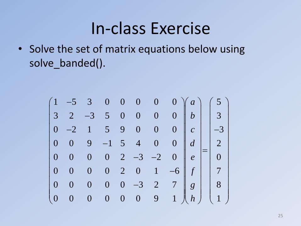
In-class Exercise • Solve the set of matrix equations below using

solve_banded().

25

1 5 3 0 0 0 0 0 5

3 2 3 5 0 0 0 0 3

0 2 1 5 9 0 0 0 3

0 0 9 1 5 4 0 0 2

0 0 0 0 2 3 2 0 0

0 0 0 0 2 0 1 6 7

0 0 0 0 0 3 2 7 8

0 0 0 0 0 0 9 1 1

a

b

c

d

e

f

g

h

In-class Results

a = 200.639937

b = -25.491352

c = -107.698899

d = -174.206761

e = 102.750000

f = 70.833333

g = -3.500000

h = 32.500000

26