equipment investment and economic growth: how strong is ... · j. bradford de long harvard...
TRANSCRIPT

J. BRADFORD DE LONG Harvard University
LAWRENCE H. SUMMERS World Bank and Harvard University
Equipment Investment
and Economic Growth:
How Strong Is the Nexus?
PRODUCTIVITY GROWTH is the important dimension of long-run eco- nomic performance. Yet economists have said relatively little about how policies affect the transcendently important long-run growth rate. Textbook theories of the type pioneered by Robert M. Solow maintain that policies cannot affect growth rates over a sufficiently long run. The growth-accounting tradition of Robert M. Solowl and Edward F. Deni- son2 has tended to conclude that most of the differences in growth are due not to differences in measured investments, but to a "residual," total factor productivity (TFP). Such models produce what Solow calls "in- vestment pessimism": radical policy changes that have large effects on investment and other resource allocations have little effect on long-run growth.3
Yet economies grow, and grow at very different rates. The TFP "re- sidual" takes on very different values in different economies. It is im-
We would like to thank members of the Brookings Panel, Robert Barro, Robert Gor- don, John Gruber, Charles Jones, Lawrence Katz, Nicholas Oulton, Lant Pritchett, Paul Romer, Charles Schultze, and especially Robert Summers for helpful discussions and comments. The opinions expressed in this paper are those of the authors and not those of the World Bank or any other organization with which the authors are affiliated.
1. Solow(1957). 2. Denison (1967). 3. Solow(1990).
157
158 Brookings Papers on Economic Activity, 2:1992
plausible that these different rates of TFP growth are entirely generated by noneconomic forces, unrelated to resource allocation decisions. If significant differences in growth are due to resource allocation decisions that affect total factor productivity, private rewards cannot be used to evaluate social returns. Thus in assessing the determinants of growth, there is little alternative to examining natural experiments provided by the different policies, investment outcomes, and growth rates found in various nations.4
In our 1991 paper, we focused on equipment investment as poten- tially a key factor in growth in a post-World War II cross section of economies spanning the range from the poorest to the richest.5 Using data from the United Nations International Comparison Project (here- after ICP),6 we distinguished between "investment effort"-current consumption forgone-and actual investment in an economy: buildings constructed and equipment put into operation. The real price of equip- ment differs by as much as a factor of four across countries, making nominal investment shares very imperfect measures of real investment. We found that countries with high equipment investment grew ex- tremely rapidly, even controlling for a number of other factors. This as- sociation suggested a causal relationship: rapid growth went with high equipment investment, no matter whether high investment was a conse- quence of high savings or of a low relative equipment price.
In this report, we extend this line of work, focusing on the experience of relatively rich high-productivity economies that had already pro- gressed far toward industrialization before our samples began. First, we verify the growth-equipment nexus using new cross-country data to demonstrate that our earlier strong results are the result neither of Dar- winian biases in specification selection nor of placing a heavy weight on the experiences of poorer developing economies, which provide few les- sons for economic policy in the rich industrial democracies. When we focus on the possibility that the growth-equipment nexus varies in
4. This is the approach taken in many recent empirical studies of growth in the "endo- genous growth theory" tradition largely sparked by Romer (1986). See Barro (1991) and the other papers published in the May 1991 Quarterly Journal of Economics (including our 1991 paper) for a sample of such work.
5. De Long and Summers (1991). 6. The ICP data is drawn from the following sources: Kravis and others (1975, 1978,
1982); OECD (1987, 1992); United Nations (1986); Ward (1985); and unpublished data pro- vided by Alan Heston, Robert Summers, and the United Nations.
J. Bradford De Long and Lawrence H. Summers 159
strength with an economy's productivity level, we find little sign that the richest nations are different from other countries in this respect. Growth-measured by labor or by TFP-is as tied to high equipment investment for rich countries as for newly industrializing ones.
Second, we present further statistical evidence suggesting that varia- tions in equipment investment arising from different sources have simi- lar impacts on growth. We support our evidence with case studies that link differences in policies toward equipment to poor performance in Argentina and impressive performance in Japan over the past few dec- ades. Third, we calculate both social rates of return to investment in equipment and the boost to total factor productivity growth associated with equipment investment. We find that equipment appears to have a very high net social return-in the range of 20 percent per year; more than half of this comes from increased TFP. We conclude that the mac- roeconomic data give no evidence that poorer economies benefit more from high rates of equipment investment than do richer economies. This suggests, significantly, large external benefits from equipment invest- ment even in rich economies. We conclude that policies that tilt the play- ing field against equipment investment are likely to be disastrous, and that a strong case exists for at least modest bias in favor of equipment investment.
The Robust Association of Equipment and Growth
There are good reasons to believe ex ante that equipment investment might have a strong association with growth. The link between technolo- gies and the capital goods in which they are embodied is a central com- ponent of economic histories.7 Steam engines were necessary for steam power, textile manufacture required power looms, and assembly line production was unthinkable without investments in the high-precision machines that made interchangeable metal parts. New technologies re- quire new types of capital. Technological change is capital-using, and TFP cannot increase without an increase in capital intensity as well.8 To
7. See Landes (1969) and Mokyr (1990). 8. See Jorgenson (1988). Note, however, that it is very difficult to attribute a large
share of differences in national rates of productivity growth to "embodiment" effects in the strict sense. Embodiment in the strict sense affects productivity only as the average age of the capital stock changes, and the average age of capital is relatively insensitive to shifts in the rate of investment. See Denison (1964).

160 Brookings Papers on Economic Activity, 2:1992
the extent that these factors lead investments in equipment to have high rates of return, they lead such investments to have high private returns and thus generate no strong case for policies to tilt the playing field.
Yet there are reasons to believe that equipment investment and growth are strongly associated through channels that would make social returns higher than private ones. One such channel that is possibly more important than embodiment or the factor-using bias of technological change is the key role that is played by experience and feedback in en- hancing economies' ability to produce efficiently using new technolo- gies. Trial-and-error and experience are the best ways to learn what works, and how what was built needs to be modified to be efficient. His- torians of technology such as David C. Mowery and Nathan Rosenberg stress that much technological knowledge is "tacit": based on hands-on experience, hard to summarize, and difficult to transmit through educa- tion.9 Such hands-on experience presupposes investments in the equip- ment upon which to learn.
The importance of trial-and-error and experience is magnified by the process of incremental adaptation needed to turn a new idea into an ef- ficient production process. Experience is the best teacher not only for the user, but also for the manufacturer and the designer of capital goods. As Rosenberg puts it, "most inventions are relatively . . . inefficient. [They are] of necessity badly adapted to many of the ultimate uses to which they will eventually be put." 10 Mowery and Rosenberg criticize those who regard innovation as "the application of 'upstream' scientific knowledge to the 'downstream' activities of new product design and . new manufacturing processes.""II In Mowery's and Rosenberg's view, "the primary sources of innovation [are] 'downstream'"; improved equipment and better ways of using them do not emerge without users to pinpoint useful modifications. 12
A similar stress on incremental improvement is found in Henry Ro- sovsky's studies of the adaptation of well-known technologies to factor intensities and resources in industrializing countries. Investigations of Japan's industrial success stress Japanese excellence in what Rosovsky calls "improvement engineering." The successful adaptation of new technologies requires capabilities to alter and modify technologies in
9. Mowery and Rosenberg (1989). 10. Rosenberg (1976, p. 195). 11. Mowery and Rosenberg (1989, p. 8). 12. Mowery and Rosenberg (1989, p. 8).
J. Bradford De Long and Lawrence H. Summers 161
many ways and often in response to local conditions, Rosovsky empha- sizes. Furthermore, new technologies often require substantial modifi- cation before they are successful. In Rosovsky's estimation, this "im- provement engineering" also requires a high degree of technical competence. 13
Such "indirect" increases in productivity can be kept proprietary only with difficulty. Workers who can use and adapt technologies can and do demand higher wages because their newly acquired skills are val- uable to firms down the street. Firms copy operating procedures from path-breaking competitors. Perhaps the most important outcome of the acquisition and use of equipment may be what the experience of install- ing and using capital teaches workers and organizations about how to use modern technologies efficiently. Such a view leads to an expectation of high social returns from equipment investment, because such invest- ment is a necessary precondition to launch this process of learning and experience. This view also suggests that good economic policy contains incentives to boost investment in equipment.
Previous Results
In our 1991 paper, we regressed growth of output per worker from 1960 to 1985 (measured in 1985 international dollars) on estimates of the share of output devoted to investment in equipment from 1960 to 1985. We used estimates of national relative price and quantity structures for benchmark years denominated in "international dollar" units from the ICP, which allows for cross-national comparisons that are orders of magnitude more accurate than previous estimates. 14 We used estimates of total investment devoted to equipment derived from benchmark-year data of Irving B. Kravis, Alan Heston, and Robert Summers and other ICP observations to estimate the share of equipment investment in GDP from 1960 to 1985. We then merged our equipment investment estimates with the cross-country comparative growth accounts of two earlier stud- ies by Summers and Heston. '5
13. Rosovsky (1972, p. 28 ff). 14. See Kravis and others (1982). 15. Summers and Heston (1988, 1991). Note that these estimates depend on the ratio
of equipment to total investment in benchmark years being a good proxy for the average ratio of equipment to total investment, and are confined to economies that served as benchmarks in the ICP.
162 Brookings Papers on Economic Activity, 2:1992
Our basic regressions controlled for labor force growth, investment in nonequipment capital, and the productivity gap vis-a-vis the world's industrial leader. Most importantly, our study took care to distinguish investment from "investment effort." Different countries have radically different price structures. The same forgone consumption purchased three times as much machinery and equipment in Japan as in Argentina in the decades following World War II.
In all probability, determinants and patterns of growth among poorer economies are very different from those of advanced industrial econo- mies. If we are concerned with the determinants of growth in industrial economies, there is good reason to pay more attention to the high- productivity countries than to the full sample. But there is a very strong association between equipment investment and growth in both samples and in regressions that include a variety of additional controls. 16 Table 1 presents results for the earlier sample of 61 non-oil-exporting nations used in our 1991 paper, and for a subset composed of high-productivity nations that by 1960 had already progressed far toward industrial- ization. 17
The estimated regression is
(1) Aln(Y/L) = PO + BI (Ieq/Y) + 12(Ist/Y) + I3 Aln(L) + 34(Y/L)o/(Y/L)OUs + e.
The average annual growth rate in output per worker, YIL, for country i is regressed on several factors: a constant; country i's average ratio of
16. Moreover, there is no sign that the very richest economies-in northwest Europe, North America, and Australia-are outliers following different laws of motion than the rest of the high-productivity sample.
17. The results shown here are numerically different from those reported in our 1991 paper because we have corrected two data errors. We thank Nicholas Oulton for uncov- ering these flaws in our dataset. Included in table 1 are regressions adding primary and secondary school enrollment rates in 1960, as well as continent dummies, to our basic inde- pendent variables. Of the differences between continent dummies, only two are statisti- cally significant: the differences between Africa and Europe (1.6 percentage points per year, with a t-statistic of 1.6); and the differences between Africa and Asia (1.7 percentage points per year, with a t-statistic of 2.1). School enrollment rates are neither statistically nor substantively significant; a one percentage point increase in the primary school enroll- ment rate is associated with a boost in growth of only 0.01 percentage points per year; a one percentage point increase in the secondary school enrollment rate is associated with a boost in growth of only 0.003 percentage points per year. The high productivity sample is defined as countries with an output per worker level that is at least 20 percent of the U. S. level at either the beginning or the end of the sample period.

J. Bradford De Long and Lawrence H. Summers 163
Table 1. Basic Regression Results from De Long and Summers (1991)
High-productivity economies
Including developing economies
Including Including schooling continent
Independent variable 1960-85 1960-75 1975-85 1960-85 variables dummies
Equipment investment as 0.302 0.295 0.425 0.219 0.245 0.246 a share of GDP (0.073) (0.075) (0.105) (0.069) (0.073) (0.074)
Other investment as a 0.019 -0.056 0.047 0.097 0.058 0.041 share of GDP (0.052) (0.043) (0.059) (0.040) (0.046) (0.042)
Labor force growth 0.043 -0.081 -0.177 -0.026 0.003 0.119 (0.147) (0.197) (0.258) (0.193) (0.207) (0.256)
Productivity gap 0.032 0.049 0.014 0.020 0.029 0.031 vis-a-vis USA (0.009) (0.013) (0.016) (0.009) (0.013) (0.012)
Summary statistic R 2 0.719 0.593 0.428 0.369 0.406 0.484 SER (0.008) (0.009) (0.013) (0.013) (0.012) (0.012) Sample size 25 25 25 61 61 61
Source: Authors' calculations based on De Long and Summers (1991). Numbers in parentheses are standard errors. The dependent variable is the average annual growth rate in output per worker. See the text for a general specification of the regression equation. High-productivity economies are defined as having output per worker levels at least one- fifth the U.S. level at the beginning or end of the sample period.
equipment investment, Ieq'Y, to GDP for country i; its average ratio of nonequipment investment to GDP, I,,IY; its labor force growth rate, Aln(L); and the initial relative productivity gap at the start of the sample period vis-a-vis the United States, (YIL)01(YIL)us.
On the basis of the high-productivity regressions, an increase of three or four percentage points in the share of GDP devoted to equipment in- vestment is associated with an increase in GDP per worker growth of 1 percent per year. Differences in equipment investment account in a sta- tistical sense for much of the growth performance of fast- or slow-grow- ing nations. Japan achieved a growth rate edge of 2.2 percent per year from 1960 to 1985 relative to the average pattern. Conversely, Argentina has suffered a growth deficit of 2.1 percent per year. More than four- fifths of this difference is accounted for by high or low equipment in- vestment.
New Sample Periods
THE 1950s. The comparative performance of economies in the 1950s provides a source of information on the strength of the growth-equip- ment investment nexus that we did not tap in our 1991 paper. We have
164 Brookings Papers on Economic Activity, 2:1992
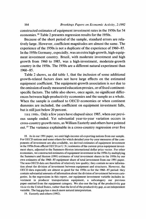
constructed estimates of equipment investment rates in the 1950s for 54 economies.'8 Table 2 presents regression results for the 1950s.
Because of the short period of the sample, standard errors are rela- tively large. However, coefficient magnitudes are almost the same. The experience of the 1950s is not a duplicate of the experience of 1960-85. In the 1950s Germany, especially, was an extra high-growth, high-equip- ment investment country. Brazil, with moderate investment and high growth from 1960 to 1985, was a high-investment, moderate-growth country in the 1950s. The 1950s are a different natural experiment than 1960-85.
Table 2 shows, as did table 1, that the inclusion of some additional growth-related factors does not have large effects on the estimated equipment coefficient. The equipment-growth association is not due to the omission of easily measured education proxies, or of fixed continent- specific factors. The table also shows, once again, no significant differ- ences between high-productivity economies and the sample as a whole. When the sample is confined to OECD economies or when continent dummies are included, the coefficient on equipment investment falls, but is still just below 20 percent.
THE 1980s. Only a few years have elapsed since 1985, when our previ- ous sample ended. Yet substantial year-to-year variation occurs in cross-country growth rates, as William Easterly and others have pointed out. '9 The variance explainable in a cross-country regression over five
18. As in our 1991 paper, we omit high-income oil-exporting nations from our sample. For OECD nations and some others for which detailed year-by-year measures of the com- ponents of investment are also available, we derived estimates of equipment investment in the 1950s from official OECD (or U.N.) estimates of the current-price equipment invest- ment share, adjusted to the Summers-Heston international dollar price vector. For other economies, we constructed estimates of equipment investment in the 1950s by multiplying the Summers and Heston (1991) estimates of total investment shares in the 1950s by our own estimates of the 1960-85 equipment share of total investment from our 1991 paper. The non-OECD data are therefore of relatively low quality; they contain no new informa- tion about the division of investment between equipment and structures. However, the OECD data especially are almost as good for the 1950s as for the 1960-85 period: they contain substantial amounts of information about the division of investment between cate- gories. In the regressions in this report, our equipment investment variable includes in- vestment in producer transportation equipment, a subcategory our previous paper omitted from the equipment category. We also use the log of the productivity gap vis-a-vis the United States, rather than the level of the productivity gap, as an independent variable. The log gap has a much more natural interpretation.
19. Easterly and others (1992).
J. Bradford De Long and Lawrence H. Summers 165
Table 2. Growth Regressions for the 1950s
High-productivity economiesa
Including Including Basic schooling continent All OECD
Independent variable specifications variablesb dummies economies economies
Equipment investment 0.343 0.372 0.187 0.275 0.177 (0.112) (0.158) (0.123) (0.108) (0.117)
Other investment 0.016 -0.005 -0.010 0.043 0.061 (0.055) (0.062) (0.056) (0.050) (0.060)
Log productivity gap 0.021 0.023 0.020 0.007 0.021 vis-a-vis USAC (0.006) (0.006) (0.007) (0.003) (0.004)
Labor force growth -0.042 0.019 0.359 -0.372 0.249 (0.236) (0.272) (0.333) (0.222) (0.233)
Primary school 0.021 enrollment (0.017)
Secondary school -0.010 enrollment (0.021)
Summary statistic R2 0.289 0.475 0.506 0.686 0.682 SER 0.0159 0.0137 0.0138 0.0118 0.0097 Sample size 54 31 31 31 21
Source: Authors' calculations using Summers and Heston (1991) and their unpublished data; ICP data; and OECD National Accounits Statistics (various years) for estimates of equipment investment in the 1950s. Numbers in parentheses are standard errors. The dependent variable is the average annual growth rate in output per worker.
a. Economies with 1950 or 1960 output per worker levels at least one-fifth that of the United States. b. Primary and secondary enrollment rates as a fraction of the school-age population. c. The log productivity gap is used in this table and subsequent ones rather than the productivity gap because the
coefficient on the gap in log productivity has a much more straightforward interpretation: a coefficient of 0.02 means that 2 percent of the log productivity gap is closed with each year, or that (0.02 x 25) = 50 percent of the gap is closed over a 25-year period.
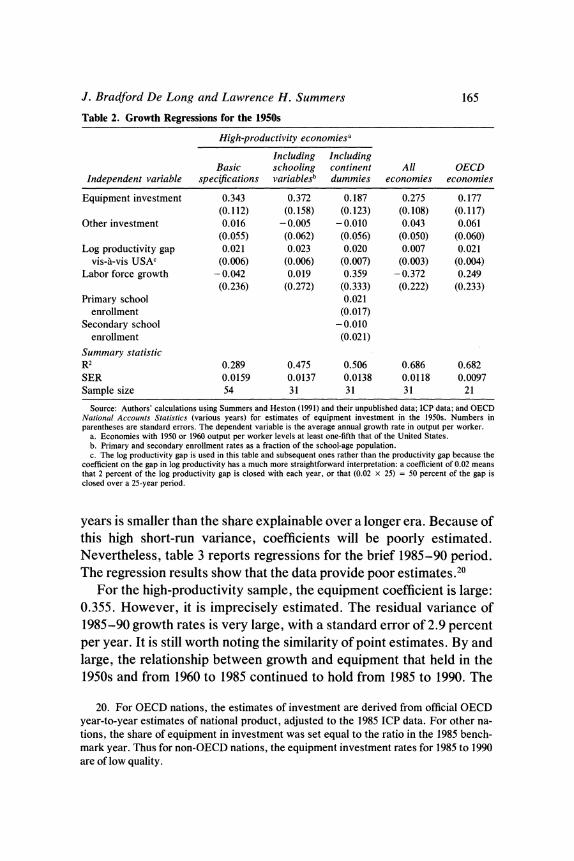
years is smaller than the share explainable over a longer era. Because of this high short-run variance, coefficients will be poorly estimated. Nevertheless, table 3 reports regressions for the brief 1985-90 period. The regression results show that the data provide poor estimates.20
For the high-productivity sample, the equipment coefficient is large: 0.355. However, it is imprecisely estimated. The residual variance of 1985-90 growth rates is very large, with a standard error of 2.9 percent per year. It is still worth noting the similarity of point estimates. By and large, the relationship between growth and equipment that held in the 1950s and from 1960 to 1985 continued to hold from 1985 to 1990. The
20. For OECD nations, the estimates of investment are derived from official OECD year-to-year estimates of national product, adjusted to the 1985 ICP data. For other na- tions, the share of equipment in investment was set equal to the ratio in the 1985 bench- mark year. Thus for non-OECD nations, the equipment investment rates for 1985 to 1990 are of low quality.
166 Brookings Papers on Economic Activity, 2:1992
Table 3. Growth Regressions, 1985-90
High-productivity economies
Including Including Basic continent schooling All OECD
Independent variable specification dummies variables economies economies
Equipment investment 0.355 0.088 0.331 0.217 0.114 (0.246) (0.262) (0.260) (0.184) (0.155)
Other investment 0.064 0.073 0.063 0.115 0.040 (0.109) (0.106) (0.104) (0.075) (0.131)
Log productivity gap 0.050 0.038 0.052 0.007 - 0.015 vis-a-vis USA (0.016) (0.018) (0.019) (0.005) (0.016)
Labor force growth -2.221 -3.119 -2.153 - 1.176 - 0.746 (0.529) (0.717) (0.557) (0.406) (0.697)
Summary statistic R 2 0.377 0.510 0.382 0.248 0.216 SER 0.0290 0.0277 0.0297 0.0290 0.0128 Sample size 42 42 42 71 17
Source: Authors' calculations using Summers and Heston (1991) and their unpublished data, and extended using unpublished post-1988 estimates of economic growth from the World Bank. Numbers in parentheses are standard errors. The dependent variable is the average annual growth rate in output per worker. High-productivity economies have 1985 output per worker levels at least one-fifth the U.S. level.
relationships estimated from 1960 to 1985 data do well at forecasting growth from 1985 to 1990.
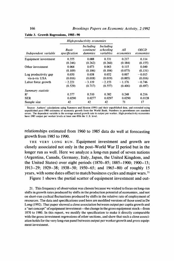
THE VERY LONG RUN. Equipment investment and growth are closely associated not only in the post-World War II period but in the longer run as well. Here we analyze a long-run panel of seven nations (Argentina, Canada, Germany, Italy, Japan, the United Kingdom, and the United States) over eight periods (1870-85; 1885-1900; 1900-13; 1913-29; 1929-38; 1938-50; 1950-65; and 1965-80) of roughly 15 years, with some dates offset to match business cycles and major wars.2'
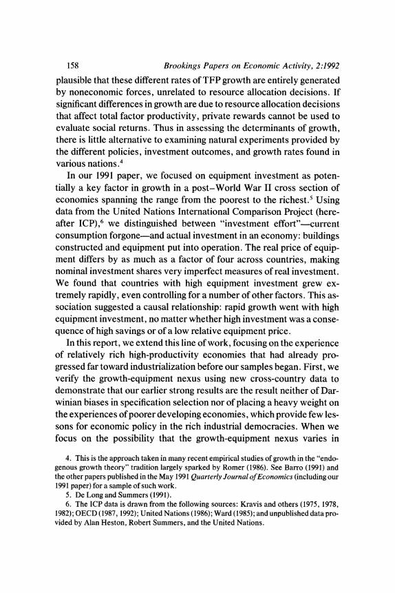
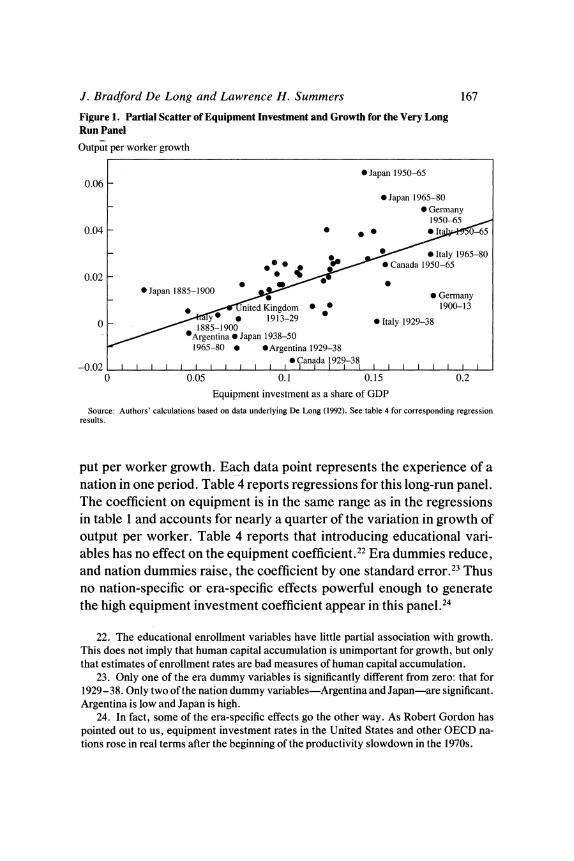
Figure 1 shows the partial scatter of equipment investment and out-
21. This frequency of observation was chosen because we wished to focus on long-run shifts in growth rates produced by shifts in the production potential of economies, and not on short-run cyclical fluctuations produced by shifts in the relative rate of employment of resources. The data and specifications used here are modified versions of those used in De Long (1992). That paper showed a close association between output per capita growth and a "net concept" of equipment investment-the change in the gross equipment stock-from 1870 to 1980. In this report, we modify the specification to make it directly comparable with the gross investment regressions of other sections, and show that such a close associ- ation holds for the very long-run panel between output per worker growth and gross equip- ment investment.
J. Bradford De Long and Lawrence H. Summers 167
Figure 1. Partial Scatter of Equipment Investment and Growth for the Very Long Run Panel Output per worker growth
*Japan 1950-65 0.06 -
*Japan 1965-80 - 0 Germany
1950-65 0.04 - 0 0 t 0-5
0 Italy 1965-80 0. 02 * Canada 1950-65
0.02 * Japan 1885-1900 0 Germany
n ited Kingdom * 1900s13 1913-29~~~~~~1001
0 85-1900 0 Italy 1929-38
*Argentina * Japan 1938-50 ~~~~~1965-80 * *Argentina 1929-38
-0.02~~~~~~~~~~ *Canada 1929-38llllllll 0 0.05 0.1 0.15 0.2
Equipment investment as a share of GDP
Source: Authors' calculations based on data underlying De Long (1992). See table 4 for corresponding regression results.
put per worker growth. Each data point represents the experience of a nation in one period. Table 4 reports regressions for this long-run panel. The coefficient on equipment is in the same range as in the regressions in table 1 and accounts for nearly a quarter of the variation in growth of output per worker. Table 4 reports that introducing educational vari- ables has no effect on the equipment coefficient.22 Era dummies reduce, and nation dummies raise, the coefficient by one standard error.23 Thus no nation-specific or era-specific effects powerful enough to generate the high equipment investment coefficient appear in this panel.24
22. The educational enrollment variables have little partial association with growth. This does not imply that human capital accumulation is unimportant for growth, but only that estimates of enrollment rates are bad measures of human capital accumulation.
23. Only one of the era dummy variables is significantly different from zero: that for 1929- 38. Only two of the nation dummy variables-Argentina and Japan-are significant. Argentina is low and Japan is high.
24. In fact, some of the era-specific effects go the other way. As Robert Gordon has pointed out to us, equipment investment rates in the United States and other OECD na- tions rose in real terms after the beginning of the productivity slowdown in the 1970s.
168 Brookings Papers on Economic Activity, 2:1992
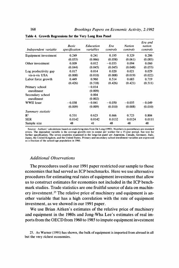
Table 4. Growth Regressions for the Very Long Run Panel
Era and Basic Education Era Nation nation
Independent variable specification variables controls controls controls
Equipment investment 0.249 0.241 0.195 0.329 0.286 (0.055) (0.066) (0.058) (0.061) (0.083)
Other investment 0.009 0.012 -0.033 0.094 0.060 (0.044) (0.045) (0.045) (0.048) (0.053)
Log productivity gap 0.017 0.014 0.020 0.021 0.029 vis-a-vis USA (0.008) (0.010) (0.008) (0.019) (0.022)
Labor force growth 0.449 0.960 0.514 0.683 0.719 (0.426) (0.518) (0.426) (0.421) (0.511)
Primary school -0.014 enrollment (0.009)
Secondary school 0.004 enrollment (0.002)
WWII loser -0.038 -0.041 - 0.050 -0.035 -0.049 (0.009) (0.009) (0.010) (0.008) (0.010)
Summary statistic R2 0.531 0.623 0.666 0.723 0.804 SER 0.0142 0.0142 0.0132 0.0124 0.0111 Sample size 48 41 48 48 48
Source: Authors' calculations based on underlying data from De Long (1992). Numbers in parentheses are standard errors. The dependent variable is the average growth rate in output per worker for a 15-year period. See text for further specification. The seven countries examined in the long-run panel are Argentina, Canada, Germany, Italy, Japan, the United Kingdom, and the United States. Primary and secondary school enrollment variables are expressed as a fraction of the school-age population in 1960.
Additional Observations
The procedures used in our 1991 paper restricted our sample to those economies that had served as ICP benchmarks. Here we use alternative procedures for estimating real rates of equipment investment that allow us to construct estimates for economies not included in the ICP bench- mark studies. Trade statistics are one fruitful source of data on machin- ery investment.25 The relative price of machinery and equipment is an- other variable that has a high correlation with the rate of equipment investment, as we showed in our 1991 paper.
We use Brian Aitken's estimates of the relative price of machinery and equipment in the 1980s and Jong-Wha Lee's estimates of real im- ports from the OECD from 1960 to 1985 to impute equipment investment
25. As Warner (1991) has shown, the bulk of equipment is imported from abroad in all but the very richest economies.
J. Bradford De Long and Lawrence H. Summers 169
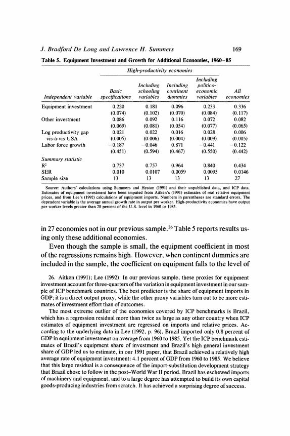
Table 5. Equipment Investment and Growth for Additional Economies, 1960-85
High-productivity economies
Including Including Including politico-
Basic schooling continent economic All Independent variable specifications variables dummies variables economies
Equipment investment 0.220 0.181 0.096 0.233 0.336 (0.074) (0.102) (0.070) (0.084) (0.117)
Other investment 0.086 0.092 0.116 0.072 0.082 (0.069) (0.081) (0.054) (0.077) (0.065)
Log productivity gap 0.021 0.022 0.016 0.028 0.006 vis-a-vis USA (0.005) (0.006) (0.004) (0.009) (0.005)
Labor force growth -0.187 -0.046 0.871 -0.441 -0.122 (0.451) (0.594) (0.467) (0.550) (0.442)
Summary statistic R 2 0.737 0.757 0.964 0.840 0.434 SER 0.010 0.0107 0.0059 0.0095 0.0146 Sample size 13 13 13 13 27
Source: Authors' calculations using Summers and Heston (1991) and their unpublished data, and ICP data. Estimates of equipment investment have been imputed from Aitken's (1991) estimates of real relative equipment prices, and from Lee's (1992) calculations of equipment imports. Numbers in parentheses are standard errors. The dependent variable is the average annual growth rate in output per worker. High-productivity economies have output per worker levels greater than 20 percent of the U.S. level in 1960 or 1985.
in 27 economies not in our previous sample.26 Table 5 reports results us- ing only these additional economies.
Even though the sample is small, the equipment coefficient in most of the regressions remains high. However, when continent dummies are included in the sample, the coefficient on equipment falls to the level of
26. Aitken (1991); Lee (1992). In our previous sample, these proxies for equipment investment account for three-quarters of the variation in equipment investment in our sam- ple of ICP benchmark countries. The best predictor is the share of equipment imports in GDP; it is a direct output proxy, while the other proxy variables turn out to be more esti- mates of investment effort than of outcomes.
The most extreme outlier of the economies covered by ICP benchmarks is Brazil, which has a regression residual more than twice as large as any other country when ICP estimates of equipment investment are regressed on imports and relative prices. Ac- cording to the underlying data in Lee (1992, p. 96), Brazil imported only 0.8 percent of GDP in equipment investment on average from 1960 to 1985. Yet the ICP benchmark esti- mates of Brazil's equipment share of investment and Brazil's high general investment share of GDP led us to estimate, in our 1991 paper, that Brazil achieved a relatively high average rate of equipment investment: 4.1 percent of GDP from 1960 to 1985. We believe that this large residual is a consequence of the import-substitution development strategy that Brazil chose to follow in the post-World War II period. Brazil has eschewed imports of machinery and equipment, and to a large degree has attempted to build its own capital goods-producing industries from scratch. It has achieved a surprising degree of success.
170 Brookings Papers on Economic Activity, 2:1992
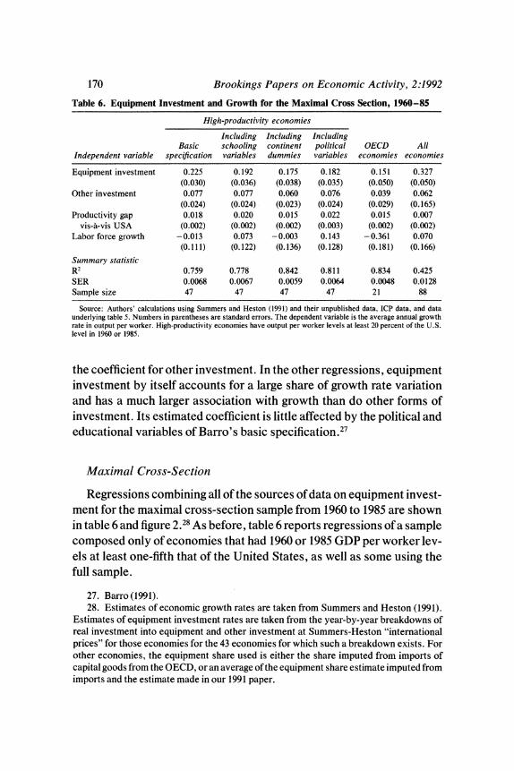
Table 6. Equipment Investment and Growth for the Maximal Cross Section, 1960-85
High-productivity economies
Including Including Including Basic schooling continent political OECD All
Independent variable specification variables dummies variables economies economies
Equipment investment 0.225 0.192 0.175 0.182 0.151 0.327 (0.030) (0.036) (0.038) (0.035) (0.050) (0.050)
Other investment 0.077 0.077 0.060 0.076 0.039 0.062 (0.024) (0.024) (0.023) (0.024) (0.029) (0.165)
Productivity gap 0.018 0.020 0.015 0.022 0.015 0.007 vis-A-vis USA (0.002) (0.002) (0.002) (0.003) (0.002) (0.002)
Labor force growth -0.013 0.073 -0.003 0.143 -0.361 0.070 (0.111) (0.122) (0.136) (0.128) (0.181) (0.166)
Summary statistic R2 0.759 0.778 0.842 0.811 0.834 0.425 SER 0.0068 0.0067 0.0059 0.0064 0.0048 0.0128 Sample size 47 47 47 47 21 88
Source: Authors' calculations using Summers and Heston (1991) and their unpublished data, ICP data, and data underlying table 5. Numbers in parentheses are standard errors. The dependent variable is the average annual growth rate in output per worker. High-productivity economies have output per worker levels at least 20 percent of the U.S. level in 1960 or 1985.
the coefficient for other investment. In the other regressions, equipment investment by itself accounts for a large share of growth rate variation and has a much larger association with growth than do other forms of investment. Its estimated coefficient is little affected by the political and educational variables of Barro's basic specification.27
Maximal Cross-Section
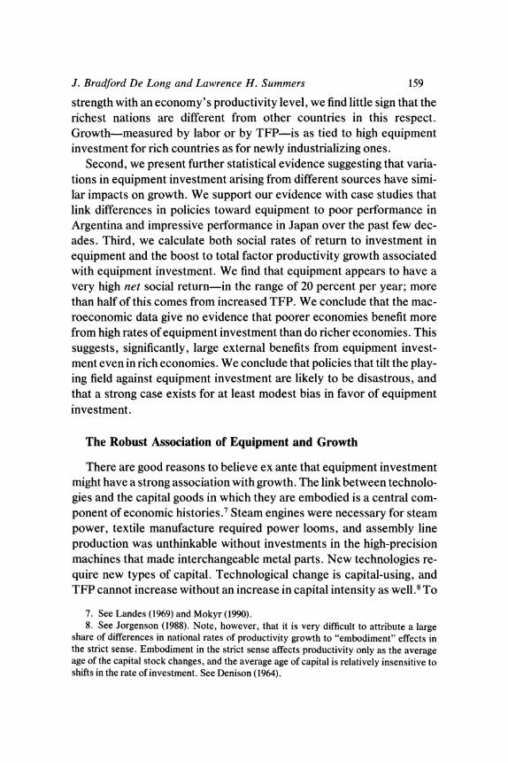
Regressions combining all of the sources of data on equipment invest- ment for the maximal cross-section sample from 1960 to 1985 are shown in table 6 and figure 2.28 As before, table 6 reports regressions of a sample composed only of economies that had 1960 or 1985 GDP per worker lev- els at least one-fifth that of the United States, as well as some using the full sample.
27. Barro(1991). 28. Estimates of economic growth rates are taken from Summers and Heston (1991).
Estimates of equipment investment rates are taken from the year-by-year breakdowns of real investment into equipment and other investment at Summers-Heston "international prices" for those economies for the 43 economies for which such a breakdown exists. For other economies, the equipment share used is either the share imputed from imports of capital goods from the OECD, or an average of the equipment share estimate imputed from imports and the estimate made in our 1991 paper.
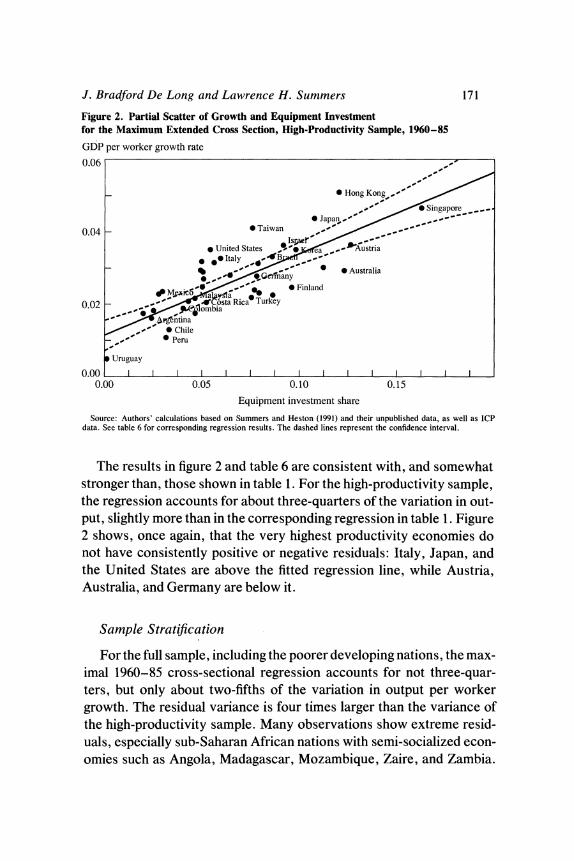
J. Bradford De Long and Lawrence H. Summers 171
Figure 2. Partial Scatter of Growth and Equipment Investment for the Maximum Extended Cross Section, High-Productivity Sample, 1960-85 GDP per worker growth rate
0.06
r~~~~~~~~~~~~~~4 Hong Kong /
," Sin~gapore ____- * Japan,',_~
0.04 - Taiwan ,, / ,,,,
* United States * ' ea -Austria * *eItaly . 4B
- ,,,Gc -any * 0 Australia
# Mplet;,yfla ' 0 Finland
0.02 - ;;g ?1bo Rica Turkey
-,,' * ~Peru
0 Uruguay
0.00 I I I I I I I I I I I I I ,1 I I
0.00 0.05 0.10 0.15
Equipment investment share
Source: Authors' calculations based on Summers and Heston (1991) and their unpublished data, as well as ICP data. See table 6 for corresponding regression results. The dashed lines represent the confidence interval.
The results in figure 2 and table 6 are consistent with, and somewhat stronger than, those shown in table 1. For the high-productivity sample, the regression accounts for about three-quarters of the variation in out- put, slightly more than in the corresponding regression in table 1. Figure 2 shows, once again, that the very highest productivity economies do not have consistently positive or negative residuals: Italy, Japan, and the United States are above the fitted regression line, while Austria, Australia, and Germany are below it.
Sample Stratification
For the full sample, including the poorer developing nations, the max- imal 1960-85 cross-sectional regression accounts for not three-quar- ters, but only about two-fifths of the variation in output per worker growth. The residual variance is four times larger than the variance of the high-productivity sample. Many observations show extreme resid- uals, especially sub-Saharan African nations with semi-socialized econ- omies such as Angola, Madagascar, Mozambique, Zaire, and Zambia.
172 Brookings Papers on Economic Activity, 2:1992
In samples that include the poorer developing economies, equipment in- vestment and the other three basic variables do not provide us with a comprehensive explanation for growth; significant dimensions of varia- tion remain unaccounted for. This pattern-a significantly tighter fit and higher R2 when the poorer developing economies are omitted from the sample-suggests a structural break in at least the magnitude of other residual influences between the poorer and the better-off economies. This is perhaps due to the poorer quality of the data for developing econ- omies, but more likely due to the existence of other important omitted factors driving growth.
Within the high-productivity sample, considerable heterogeneity oc- curs as well. The sample includes newly industrializing economies such as Taiwan; economies such as Argentina that have seen a prolonged period of relative decline; peripheral European economies such as Por- tugal that are rapidly integrating themselves into western Europe; and the advanced industrial economies of the world's economic core.
The implications for U.S. or G-7 economic policy are considerably less interesting if the finding of a close association between high equip- ment investment and rapid growth is driven solely by the experience of newly industrializing economies. Could it be that economies with rela- tively low productivity gain substantially from high equipment invest- ment, while richer economies that are already near the forefront of the world's best practice production processes do not?
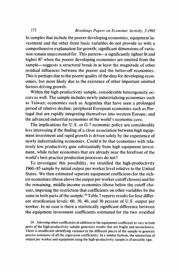
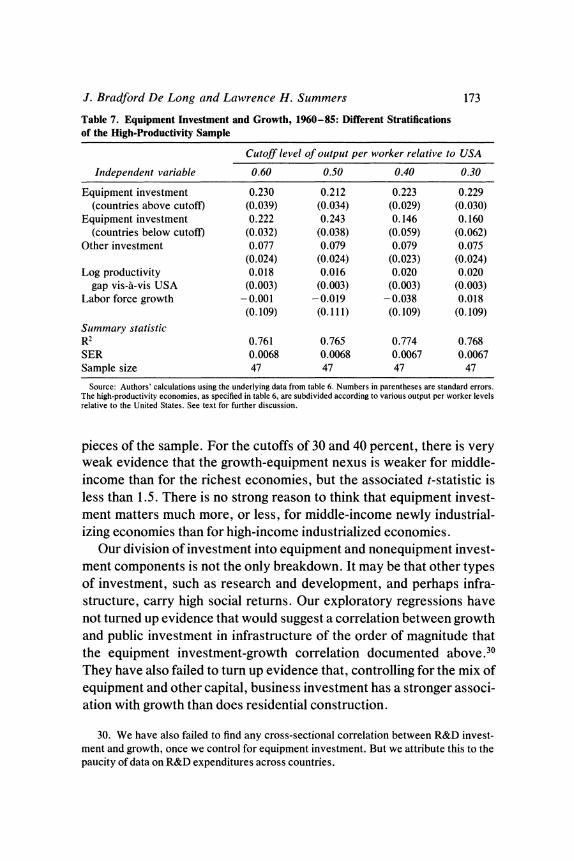
To investigate this possibility, we stratified the high-productivity 1960-85 sample by initial output per worker level relative to the United States. We then estimated separate equipment coefficients for the rich- est economies (those above the output per worker cutoff chosen) and for the remaining, middle-income economies (those below the cutoff cho- sen), imposing the restriction that coefficients on other variables be the same in both parts of the sample.29 Table 7 reports results for four differ- ent stratification levels: 60, 50, 40, and 30 percent of U.S. output per worker. In no case is there a statistically significant difference between the equipment investment coefficients estimated for the two stratified
29. Allowing other coefficients in addition to the equipment coefficient to vary in both parts of the high-productivity sample generates results that are fragile and inconclusive. There is insufficient identifying variance in the different pieces of the sample to generate precise estimates of all the regression coefficients. In a similar fashion, the interaction of output per worker and equipment using the high-productivity sample is of unstable sign.
J. Bradford De Long and Lawrence H. Summers 173
Table 7. Equipment Investment and Growth, 1960-85: Different Stratifications of the High-Productivity Sample
Cutoff level of output per worker relative to USA
Independent variable 0.60 0.50 0.40 0.30
Equipment investment 0.230 0.212 0.223 0.229 (countries above cutoff) (0.039) (0.034) (0.029) (0.030)
Equipment investment 0.222 0.243 0.146 0.160 (countries below cutoff) (0.032) (0.038) (0.059) (0.062)
Other investment 0.077 0.079 0.079 0.075 (0.024) (0.024) (0.023) (0.024)
Log productivity 0.018 0.016 0.020 0.020 gap vis-a-vis USA (0.003) (0.003) (0.003) (0.003)
Labor force growth -0.001 -0.019 -0.038 0.018 (0. 109) (0.111) (0.109) (0. 109)
Summary statistic R 2 0.761 0.765 0.774 0.768 SER 0.0068 0.0068 0.0067 0.0067 Sample size 47 47 47 47
Source: Authors' calculations using the underlying data from table 6. Numbers in parentheses are standard errors. The high-productivity economies, as specified in table 6, are subdivided according to various output per worker levels relative to the United States. See text for further discussion.
pieces of the sample. For the cutoffs of 30 and 40 percent, there is very weak evidence that the growth-equipment nexus is weaker for middle- income than for the richest economies, but the associated t-statistic is less than 1.5. There is no strong reason to think that equipment invest- ment matters much more, or less, for middle-income newly industrial- izing economies than for high-income industrialized economies.
Our division of investment into equipment and nonequipment invest- ment components is not the only breakdown. It may be that other types of investment, such as research and development, and perhaps infra- structure, carry high social returns. Our exploratory regressions have not turned up evidence that would suggest a correlation between growth and public investment in infrastructure of the order of magnitude that the equipment investment-growth correlation documented above.30 They have also failed to turn up evidence that, controlling for the mix of equipment and other capital, business investment has a stronger associ- ation with growth than does residential construction.
30. We have also failed to find any cross-sectional correlation between R&D invest- ment and growth, once we control for equipment investment. But we attribute this to the paucity of data on R&D expenditures across countries.
174 Brookings Papers on Economic Activity, 2:1992
To the extent that our data are able to distinguish among breakdowns of investment into different sets of components, equipment investment does have a uniquely strong association with growth. But attempting to distinguish between different potential breakdowns of investment car- ries us to, or perhaps beyond, the power of our macroeconomic dataset to discriminate among possibilities.
All samples and periods we have surveyed carry the same message. Regressions using new data, whether covering new periods or addi- tional economies, strongly confirm our previous finding that the growth- equipment nexus is strong. Whether we examine the cross-sectional re- gression covering the 1950s, the results for the 1985-90 period, the very long-run panel, or the regressions run on additional economies, we have not found any strong differences in the strength of the growth-equipment relationship in samples stratified by productivity level.3' We have not found other breakdowns of investment into components that do equally well at accounting for differences in growth rates. If a strong growth- equipment association is not a robust "stylized fact," but instead a prod- uct of some specific peculiarity or feature of our previous data, these tests of our specifications using new data should have revealed their fra- gility. They did not do so.
How Should We Interpret the Growth-Equipment Nexus?
The strong association between equipment investment and growth could arise if some other important growth-causing factor that happens to be correlated with equipment investment were omitted from the set of independent variables. Thus a high equipment investment coefficient does not necessarily imply a strong structural association of equipment with growth.
The continued strength of equipment investment when measure- ments of additonal factors are added to the right-hand side of the equa- tion (as in table 6) does not eliminate the possibility that equipment is a proxy for one or more of these factors. Our measurements are all noisy.
31. However, we have found a large difference in the fraction of growth rate variation accounted for; our regressions account for a smaller share of variation in samples that in- clude poorer economies.
J. Bradford De Long and Lawrence H. Summers 175
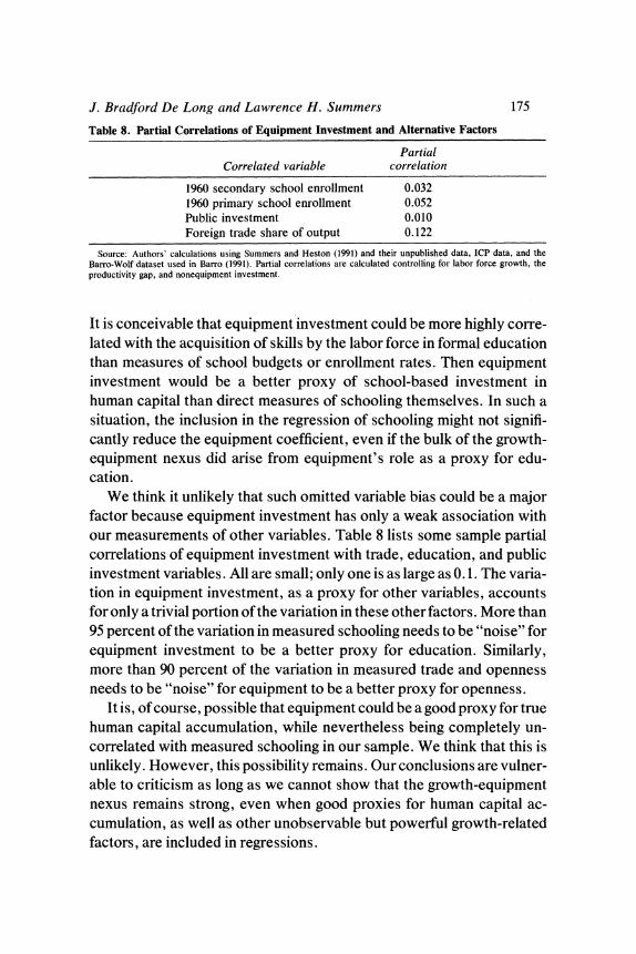
Table 8. Partial Correlations of Equipment Investment and Alternative Factors
Partial Correlated variable correlation
1960 secondary school enrollment 0.032 1960 primary school enrollment 0.052 Public investment 0.010 Foreign trade share of output 0.122
Source: Authors' calculations using Summers and Heston (1991) and their unpublished data, ICP data, and the Barro-Wolf dataset used in Barro (1991). Partial correlations are calculated controlling for labor force growth, the productivity gap, and nonequipment investment.
It is conceivable that equipment investment could be more highly corre- lated with the acquisition of skills by the labor force in formal education than measures of school budgets or enrollment rates. Then equipment investment would be a better proxy of school-based investment in human capital than direct measures of schooling themselves. In such a situation, the inclusion in the regression of schooling might not signifi- cantly reduce the equipment coefficient, even if the bulk of the growth- equipment nexus did arise from equipment's role as a proxy for edu- cation.
We think it unlikely that such omitted variable bias could be a major factor because equipment investment has only a weak association with our measurements of other variables. Table 8 lists some sample partial correlations of equipment investment with trade, education, and public investment variables. All are small; only one is as large as 0.1. The varia- tion in equipment investment, as a proxy for other variables, accounts for only a trivial portion of the variation in these other factors. More than 95 percent of the variation in measured schooling needs to be "noise" for equipment investment to be a better proxy for education. Similarly, more than 90 percent of the variation in measured trade and openness needs to be "noise" for equipment to be a better proxy for openness.
It is, of course, possible that equipment could be a good proxy for true human capital accumulation, while nevertheless being completely un- correlated with measured schooling in our sample. We think that this is unlikely. However, this possibility remains. Our conclusions are vulner- able to criticism as long as we cannot show that the growth-equipment nexus remains strong, even when good proxies for human capital ac- cumulation, as well as other unobservable but powerful growth-related factors, are included in regressions.
176 Brookings Papers on Economic Activity, 2:1992
Is the Association Causal?
It is conceivable that a strong association between investment and growth represents reverse causation running from fast growth to high investment. It is less plausible that such reverse causation would induce a strong partial association between growth and equipment investment without inducing a strong partial association between growth and struc- tures investment. Accelerator effects work on structures as powerfully as they work on equipment. In addition, our 1991 paper found that the strong correlation between growth and equipment investment was a cor- relation between intensive growth (growth in productivity holding popu- lation constant) and equipment. Extensive growth (increases in popula- tion, holding productivity constant) did not have a differentially strong association with investment in equipment, as opposed to investment in structures.
P R I C E S A N D Q U A N T I T I E S. We believe that the most powerful piece of evidence for attributing causal significance to the equipment-growth nexus is the negative association between equipment prices on the one hand and equipment investment and growth on the other. If high rates of investment were a consequence, rather than a cause of growth, one would expect equipment prices to be higher in rapidly growing countries because of strong demand pressing on the limits of supply.
This argument is simple supply-and-demand. Fast growth could in- crease equipment investment by raising profits and shifting the derived demand for equipment to the right. This would move the economy up- ward and outward along the supply curve. In such a case, rapid growth would go together with high equipment investment and high equipment prices.32
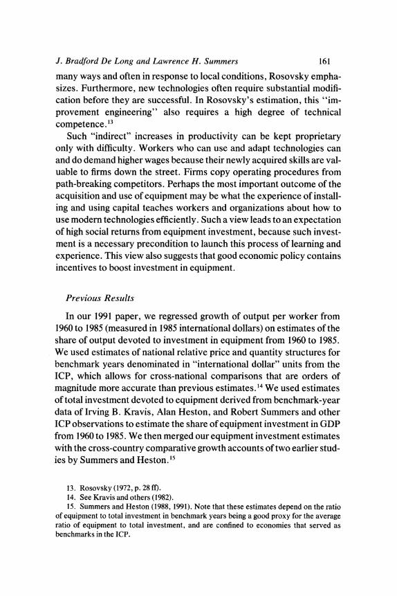
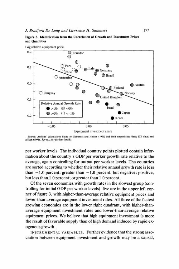
Figure 3 shows the association of equipment prices, quantities, and output per worker growth rates for 31 countries in our high-productivity sample. The vertical axis plots the relative price of machinery and equip- ment in 1980, as estimated by Aitken, controlling for current output per worker levels.33 The horizontal axis plots our estimates of 1960-85 equipment investment shares of GDP, once again controlling for output
32. If supply curves sloped downward because of economies of scale, then high de- mand could lead to low prices. However, few nations produce their own machinery and equipment. Machinery and equipment are for the most part purchased on a world market.
33. Aitken(1991).
J. Bradford De Long and Lawrence H. Summers 177
Figure 3. Identification from the Correlation of Growth and Investment Prices and Quantities
Log relative equipment price
0.2 0 Ecuador
0.1 L Peru 0 Italy
O Argent n Bai
0.0 0 (a Austria (l) F~~~~inland
? ' Uruguay UnitdK ngdom
ora -0.1 - 1 Relative Annual Growth Rate
_ >I% (D <0% Israel
-0.2 a
>0% 0 <-1% * JapX
-0.05 0.00 0.05
Equipment investment share
Source: Authors' calculations based on Summers and Heston (1991) and their unpublished data; ICP data; and Aitken (1991). See text for further details.
per worker levels. The individual country points plotted contain infor- mation about the country's GDP per worker growth rate relative to the average, again controlling for output per worker levels. The countries are sorted according to whether their relative annual growth rate is less than - 1.0 percent; greater than - 1.0 percent, but negative; positive, but less than 1.0 percent; or greater than 1.0 percent.
Of the seven economies with growth rates in the slowest group (con- trolling for initial GDP per worker levels), five are in the upper left cor- ner of figure 3, with higher-than-average relative equipment prices and lower-than-average equipment investment rates. All three of the fastest growing economies are in the lower right quadrant, with higher-than- average equipment investment rates and lower-than-average relative equipment prices. We believe that high equipment investment is more the result of favorable supply than of high demand induced by rapid ex- ogenous growth.
INSTRUMENTAL VARIABLES. Further evidence that the strong asso- ciation between equipment investment and growth may be a causal,
178 Brookings Papers on Economic Activity, 2:1992
structural association comes from instrumental variables estimates of the strength of the growth-equipment nexus. Any claim that the relation- ship running from equipment to growth is causal is a claim that a given shift in equipment investment-however engineered-will be associ- ated with a constant shift in growth. The next best thing to direct experi- mental evidence is to examine whether components of equipment in- vestment driven by different factors have the same impact on growth. We examined the relationship between growth and various components of equipment investment associated with different aspects of national economic policies.34
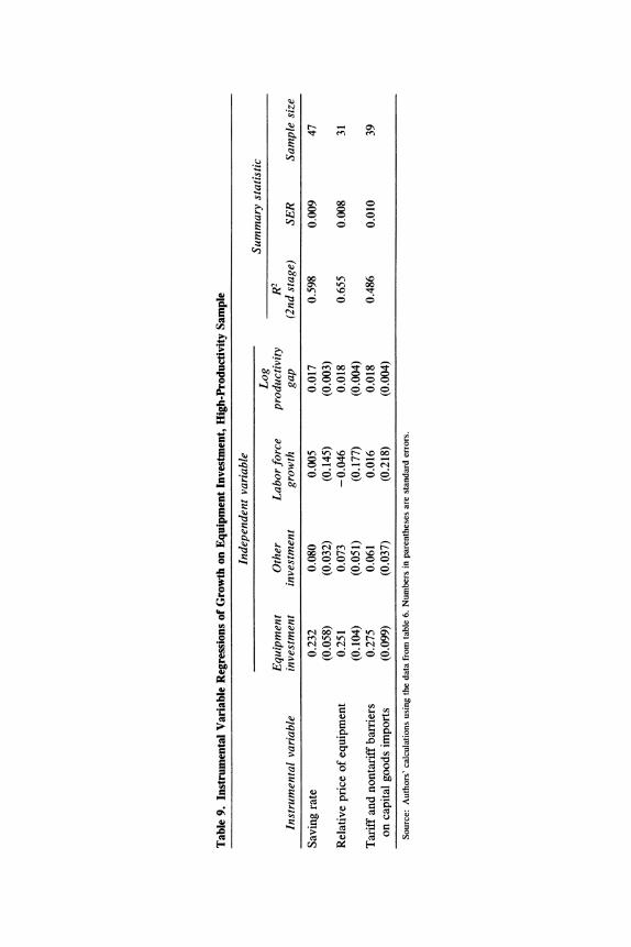
Table 9 reports regressions of growth on components of the variation in equipment investment. The coefficients measure the association be- tween growth and that portion of equipment investment correlated with the instrument. We use three sets of instruments: the average savings share of GDP from 1960 to 1985; our own estimates of the deviation of the real price of equipment from its expected value; and tariff and non- tariff barriers to equipment.
No matter which of these dimensions we examine, the association of equipment and growth remains the same. Estimated coefficients range from 0.232 to 0.275. The similarity of the association with growth for each of these components of equipment strengthens the case that the equipment-growth nexus is a "structural" relationship, not generated because equipment is a signal that other growth-producing factors are favorable.
Despite the similarity of the estimated equipment coefficients, the in- struments do capture different aspects of the variation in equipment in- vestment. The correlations among the second-stage equipment invest- ment values for the different instrumental variables regressions are not high. Controlling for nonequipment investment, the productivity gap, and labor force growth, there is a partial correlation of 0.43 between the saving-based and price-based second-stage equipment variables; of 0.45 between the price variable and the trade-barrier variables; and of only 0.28 between the saving and trade-barrier variables.
CASE STUDIES: ARGENTINA AND JAPAN. One additional line of evi- dence that the association between equipment investment and economic
34. We examined the coefficient produced by different two-stage least squares regres- sions of growth on equipment investment with different sets of instruments. This proce- dure can be viewed as an informal Hausman-Wu test of the proposition that the equipment- growth relationship is a structural one uncomplicated by omitted variables or simultaneity.
ro)
0\ 0C
zz
00 4)~ X t 00
W)W B c \ oom
?;~~~~~~~~~~c 6 ; o o
;! >. X o, .0 8,o
E z 7<3 ~~~~~~o o en o' o) o en Cu~~~~~~~~~~~~~~~~~~~J
0
0
,1 000000o,o.o.oo>
*R0: q No o.0E
= Ei- " i
180 Brookings Papers on Economic Activity, 2:1992
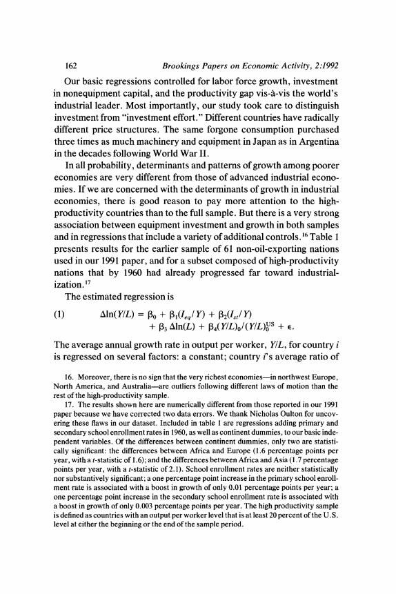
Figure 4. GDP per Capita Growth in Argentina and Europe after World War II
Index, logarithmic scale 1.5 WGm
United Kingdom ...<
0.5 - *..... . ./Italy
rFrance/ -s^ s Argentina
1950 1960 1970 1980 1990 Source: De Long and Eichengreen (1991, p. 39) based on Summers-Heston estimates.
growth is causal, and that high equipment investment is more than a sig- nal that fundamentals are attractive, comes from analyzing exemplary case studies. Here we briefly consider the disappointing economic growth of Argentina and the extraordinary growth of Japan's economy since World War II.
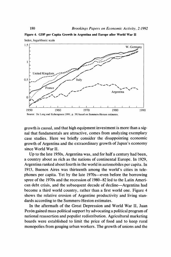
Up to the late 1950s, Argentina was, and for half a century had been, a country about as rich as the nations of continental Europe. In 1929, Argentina ranked about fourth in the world in automobiles per capita. In 1913, Buenos Aires was thirteenth among the world's cities in tele- phones per capita. Yet by the late 1970s-even before the borrowing spree of the 1970s and the recession of 1980-82 led to the Latin Ameri- can debt crisis, and the subsequent decade of decline-Argentina had become a third world country, rather than a first world one. Figure 4 shows the relative erosion of Argentine productivity and living stan- dards according to the Summers-Heston estimates.
In the aftermath of the Great Depression and World War II, Juan Peron gained mass political support by advocating a political program of national reassertion and populist redistribution. Agricultural marketing boards were established to limit the price of food and to keep rural monopolies from gouging urban workers. The growth of unions and the
J. Bradford De Long and Lawrence H. Summers 181
organization of workers were supported to allow the urban working classes a fair chance to bargain against their employers. Urban wages were boosted.
Peron's policies were popular. As Carlos F. Diaz Alejandro writes: [F]avoring domestic consumption over exports pleased the urban masses, and strengthening import restrictions pleased urban entrepreneurs. All who would lose, it appeared, were foreigners who had to do without Argentine wheat and beef and could not sell manufactures to Argentina, and the oligarchs who had previously profited from the export-import trade and their association with for- eign investors.35
Peron's policies twisted the terms of trade against rural agricultural goods and in favor of urban industrial goods. Real wages for urban work- ers and profits for urban manufacturers rose, while real incomes of rural workers and landlords fell. Imports climbed and exports dropped. By the late 1940s, the resulting foreign exchange shortage left Peron with only unattractive options. Currency controls were used to allocate newly scarce foreign exchange. The raw materials and intermediate goods needed to maintain current operations had first priority, and kept flowing. But machinery and equipment, last in the queue, could not be imported in large quantities.
The early 1950s saw a huge rise in the relative price of capital goods. Before 1948, Argentina's relative price structure had been comparable to that of Australia or New Zealand. According to the Economic Com- mission for Latin America, producer durables prices increased relative to the output deflator by more than 150 percent between 1948 and 1953. Each percentage point of national product saved produced less than half as much in terms of real investment in producer durables. A sharp de- crease in the rate of real capital formation in new machinery and equip- ment followed. According to Diaz Alejandro, the share of real producer durables investment in the 1950s was less than half what it had been even in the depressed 1930s.36
Successor governments did not reverse Peronist policies: the forces he had mobilized had to be appeased. Argentine governments through- out the post-World War II era remained committed to relative autarky, favoring urban over rural producers, terms of trade that placed rural pro- ducers at a disadvantage, overvalued exchange rates, and import con-
35. Dfaz Alejandro (1970, pp. 108-09). 36. Dfaz Alejandro (1970).
182 Brookings Papers on Economic Activity, 2:1992
trols. This produced an extraordinary rise in the relative real price of machinery and equipment-and a consequent fall in the rate of invest- ment in machinery and equipment. In Diaz Alejandro's view, this fall in investment was the principal source of slow Argentine growth after World War II. Argentina had a low TFP "residual" growth rate because it had a low rate of equipment investment: A good part of the residual arises from not fully taking into account quality changes in machinery and equipment . .. Even when technological improve- ments are not embodied in capital . .. taking full advantage . .. often requires the purchase of new machinery and equipment, while access to these capital goods will stimulate technical education and the use of better practices.37
By contrast, the economic boom in Japan since World War II has been the most extraordinary positive episode in the postwar period. Given the frequent emphasis on the strong structural differences be- tween Japan and the other industrial market economies, it is noteworthy that Japan does not have a high positive residual in our regressions: Japan's growth is about where predicted given its initial level of output per worker, its rate of investment in machinery and equipment, and the cross-sectional pattern that holds for other countries. Our regressions attribute more than 80 percent of the 4.5 percentage point per year differ- ence between Argentine and Japanese growth rates from 1960 to 1985- a difference in growth that has led Japanese output per worker to quad- ruple relative to Argentina's in a single generation-to differences in rates of equipment investment. In our regressions, differences in rela- tive starting points and in rates of equipment investment account for the entire difference between Japanese and U.S. growth rates. Thus Japan's rapid growth is attributable to its extraordinarily favorable factor supply fundamentals: its low producer goods prices and high equipment invest- ment quantities. Growth has been further boosted by favorable demo- graphics, a well-educated population, and its low post-World War II ini- tial starting point. Little is left to be attributed to any qualitative difference in economic structures.
Japan's high rate of equipment investment has many sources. A high saving rate is one. An openness to imports of technology and of foreign capital goods is another. A third, less noticed factor has been the low relative price of machinery and equipment in Japan. A large equipment investment effort-the share of national product saved and spent on
37. Dfaz Alejandro (1970, p. 83).
J. Bradford De Long and Lawrence H. Summers 183
Figure 5. Machinery and Equipment Prices and Output per Worker, 1980
Log of relative price of equipment
1.25
* Peru * Chile
1.00 Ecuador 0 * Colombia
* \ Tunisia 0.75 * Brazil
Costa R C Uruguay Costa rica\;4 gentina
0.50 * \ o Venezuela
\ o Hong Kong Itl 0.25- * Norway 0 Korea * Greece ustria
United Kingdom any United 0.00 apnUie
0 Japan States * Israel * Canada
-0.25 I l l I -1.5 -1.0 -0.5 0.0
Log of output per worker
Source: Authors' calculations using Summers and Heston (1991) and their unpublished data, and ICP data.
equipment-has been transformed into an extraordinarily large quantity of machinery and equipment investment by low relative prices of pro- ducer durables.
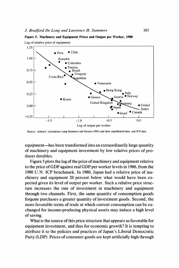
Figure 5 plots the log of the price of machinery and equipment relative to the price of GDP against real GDP per worker levels in 1980, from the 1980 U.N. ICP benchmark. In 1980, Japan had a relative price of ma- chinery and equipment 20 percent below what would have been ex- pected given its level of output per worker. Such a relative price struc- ture increases the rate of investment in machinery and equipment through two channels. First, the same quantity of consumption goods forgone purchases a greater quantity of investment goods. Second, the more favorable terms of trade at which current consumption can be ex- changed for income-producing physical assets may induce a high level of saving.
What is the source of this price structure that appears so favorable for equipment investment, and thus for economic growth? It is tempting to attribute it to the policies and practices of Japan's Liberal Democratic Party (LDP). Prices of consumer goods are kept artificially high through
184 Brookings Papers on Economic Activity, 2:1992
regulation by LDP-client bureaucracies interested in advancing the wealth of producer interests. However, the prices of producer goods are not elevated: they are not the domain of the patron-and-client-oriented LDP. Thus we would ascribe a potentially important role to the Ministry of International Trade and Industry (MITI), as a bureaucracy oriented not toward enriching the interests of producers of capital goods, but in- stead focused on achieving value for the purchasers of capital goods whose productivity is to be enhanced through investment.38 We suspect that the Japanese government, including MITI, has played a significant role in Japan's rapid growth. But we suspect that MITI has done so not by micromanaging industrial development, but by blocking the effects of politics-as-usual in the investment goods markets. The rest of the reg- ulatory bureaucracy has aided development because (unintentionally) its attempts to enrich producer interests have helped create a structure of prices and incentives in which houses are expensive, rice is costly, but equipment is cheap.
From our perspective, one of the reasons for the success of the Japa- nese economy has been that monopolistic high prices in other sectors, partially created by government action, have led to Japan's "getting rel- ative prices right." High absolute levels of other prices have pushed down the relative price of equipment, making it more "right" than would complete laissez-faire-in the sense of bringing private incentives to in- vest in equipment more closely in line with social returns.
Equipment Investment and Total Factor Productivity Growth
The correlation of equipment investment and output per worker growth implies an equally strong and almost as large a correlation be- tween equipment investment and TFP growth. The reason is straight- forward, springing from the "investment pessimism" of standard
38. Okimoto (1989, p. 5) stresses that in "most cases, such pockets of inefficiency lie outside MITI's jurisdiction." According to his analysis, LDP members seeking to transfer wealth to sectors and ministers find it easier to do so if the sector is outside the purview of the MITI ministry, with its strong interest in efficiency and development. Thus the MITI bureaucracy fulfills a valuable social role, even though the industrial policies it pursues can be badly flawed.
J. Bradford De Long and Lawrence H. Summers 185
models. Because even drastic assumptions about factor shares do not lead shifts in investment rates to have large effects on growth rates, large differences in growth rates cannot be driven by shifts in investment rates uncorrelated with TFP growth.
To make this analysis more formal, suppose that total factor produc- tivity is uncorrelated with and independent of investment. Begin with the identity
(2) AY, = (r + 8)AK,
where Y is output, r is the social net rate of return, 8 is the depreciation rate, and K is capital stock. Equation 2 simply states that the (gross) in- crease in output produced from an increase in the capital stock is the gross rate of return on capital times the increase. Suppose that an econ- omy initially in steady state receives a permanent boost, I, to its gross investment and that its capital stock evolves following
(3) AKt = I - 8Kt-1.
Equation 3 simply states that the increase in the capital stock is equal to new (gross) investment minus depreciation on last period's capital.
In the first period, the entire boost to investment will show up as an increase in the capital stock: AK, = I, and A Y, = (r + 8)I. In the second period, investment will still be running at its higher pace, boosted by I, but because K1 is higher than Ko, depreciation will be higher than it was in steady state. The increase in the capital stock will be less: AK2 =
(1 - 8)I, and A Y2 = (r + 8)(1 - 8)I. The successive increases in the capital stock will become smaller and smaller, and the sum of changes in the capital stock will converge to a steady-state value, AK*:
(4) AK* = I/8.
Thus even if we assume that r does not fall as K increases, the boost to the steady-state output level, A Y*, that can result from a permanent boost to investment is
(5) AY* = I (r + 8)18.
An increase in investment equal to one percentage point of output can thus induce no more than a (r + 8)/8 percentage point boost in the level
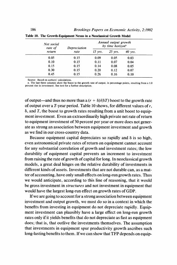
186 Brookings Papers on Economic Activity, 2:1992 Table 10. The Growth-Equipment Nexus in a Neoclassical Growth Model
Annual output growth Net social by time horizon a rate of Depreciation return rate 15 yrs. 25 yrs. 40 yrs.
0.05 0.15 0.09 0.05 0.03 0.10 0.15 0.11 0.07 0.04 0.15 0.15 0.14 0.08 0.05 0.30 0.15 0.20 0.12 0.07 0.45 0.15 0.26 0.16 0.10
Source: Based on authors' calculations. a. The last three columns show the boost to the growth rate of output, in percentage points, resulting from a 1.0
percent rise in investment. See text for a further description.
of output-and thus no more than a (r + 8)I(8T) boost to the growth rate of output over a T-year period. Table 10 shows, for different values of r, 8, and T, the boost to growth rates resulting from a unit boost to equip- ment investment. Even an extraordinarily high private net rate of return to equipment investment of 30 percent per year or more does not gener- ate as strong an association between equipment investment and growth as we find in our cross-country data.
Because equipment capital depreciates so rapidly and 8 is so high, even astronomical private rates of return on equipment cannot account for any substantial correlation of growth and investment rates; the low durability of equipment capital prevents an increment to investment from raising the rate of growth of capital for long. In neoclassical growth models, a great deal hinges on the relative durability of investments in different kinds of assets. Investments that are not durable can, as a mat- ter of accounting, have only small effects on long-run growth rates. Thus we would anticipate, according to this line of reasoning, that it would be gross investment in structures and not investment in equipment that would have the largest long-run effect on growth rates of GDP.
If we are going to account for a strong association between equipment investment and output growth, we must do so in a context in which the benefits from investing in equipment do not depreciate rapidly. Equip- ment investment can plausibly have a large effect on long-run growth rates only if it yields benefits that do not depreciate as fast as equipment does; that is, that outlive the investments themselves. The assumption that investments in equipment spur productivity growth ascribes such long-lasting benefits to them. If we can show that TFP depends on equip-
J. Bradford De Long and Lawrence H. Summers 187
ment investment, then we can account for the strong association be- tween long-run growth rates and equipment investment.39
Estimating Total Factor Productivity
Neoclassical growth theory can be viewed as either an organizing framework for thinking about growth or as a substantive theory. To the extent that it is a substantive theory, one of its most basic predictions must be that TFP growth is not associated with the principal dynamic variables-investment, depreciation, and population growth rates- about which neoclassical growth theory makes predictions. In this sub- section, we test and reject the null hypothesis that TFP growth is uncor- related with equipment investment.
It should come as no surprise that the very strong association of out- put per worker growth and equipment investment documented above is, in large part, also a strong association between equipment investment and total factor productivity growth. Given the limitations of our data- base, the calculation of total factor productivity estimates is not straight- forward. We require estimates of the average share accruing to factors of production, and estimates not of gross, but of net investment rates. Thus total factor productivity estimates require estimates of initial capi- tal stocks. Because such initial capital stock estimates are crude, they introduce a potential source of noise into TFP growth calculations.
We have estimated 1960-85 TFP growth rates for 31 of the economies in our high-productivity sample. For these 31 economies, we have year- by-year estimates of nominal investment in different types of assets and of price structures in the 1950s. Along with an assumption about pre- 1950 investment, we can construct 1960 estimates of capital stocks that can then be used to calculate total factor productivity growth from 1960 to 1985. The restriction of our total factor productivity growth estimates to 31 high-productivity economies limits us to a sample that does not show the growth-equipment nexus as strongly as some of our other sam- ples. For equations such as those in table 1, the equipment investment coefficient over the 1960-85 period is 0.198 for this particular sample, toward the low end of the range found in our later regressions.
39. One model in which TFP is a function of investment is the "creative destruction" model of Aghion and Howitt (1992).
188 Brookings Papers on Economic Activity, 2:1992
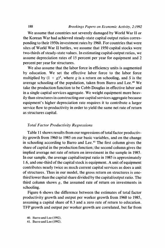
We assume that countries not severely damaged by World War II or the Korean War had achieved steady-state capital output ratios corres- ponding to their 1950s investment rates by 1960. For countries that were sites of World War II battles, we assume that 1950 capital stocks were two-thirds of steady-state values. In estimating capital-output ratios, we assume depreciation rates of 15 percent per year for equipment and 2 percent per year for structures.
We also assume that the labor force in efficiency units is augmented by education. We set the effective labor force to the labor force multiplied by (1 + g)S, where g is a return on schooling, and S is the average schooling of the population, taken from Barro and Lee.40 We take the production function to be Cobb-Douglas in effective labor and in a single capital services aggregate. We weight equipment more heav- ily than structures in constructing our capital services aggregate because equipment's higher depreciation rate requires it to contribute a larger service flow to productivity in order to yield the same net rate of return as structures capital.
Total Factor Productivity Regressions
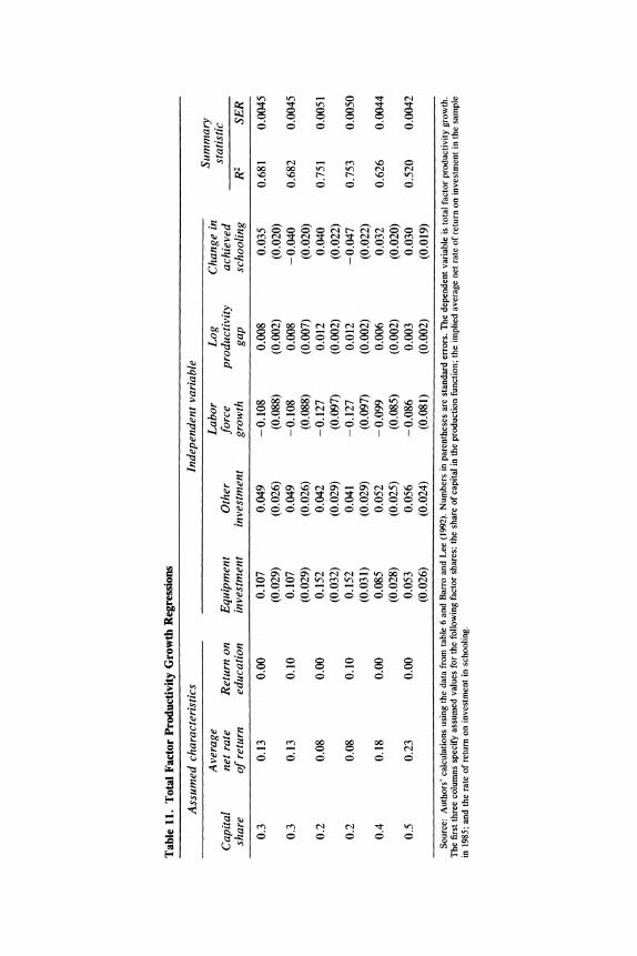
Table 11 shows results from our regressions of total factor productiv- ity growth from 1960 to 1985 on our basic variables, and on the change in schooling according to Barro and Lee.41 The first column gives the share of capital in the production function; the second column gives the implied average net rate of return on investment in the sample in 1985. In our sample, the average capital/output ratio in 1985 is approximately 1.6, and one-third of the capital stock is equipment. A unit of equipment contributes nearly twice as much current capital services as does a unit of structures. Thus in our model, the gross return on structures is one- third lower than the capital share divided by the capital/output ratio. The third column shows g, the assumed rate of return on investments in schooling.
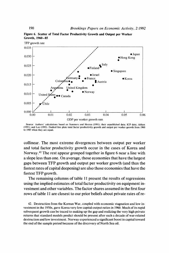
Figure 6 shows the difference between the estimates of total factor productivity growth and output per worker growth from 1960 to 1985, assuming a capital share of 0.3 and a zero rate of return to education. TFP growth and output per worker growth are correlated, but far from
40. Barro and Lee (1992). 41. BarroandLee(1992).
,I- I 0
N Nt - 06E
0 0 0 0) 0
0 00 0 01 01
- r> \C 0 osz >E
It It~ ~ t
.t~~~ N \C ib iNooo
O t a Y0 06 Y0 0 N O N 06 ?0 60 0 0C .
00000000000
- 00r' 0 0 0 N O (1 O (o1 o ? 4
0 0 ~0 0 0 C)C) ) C C)
tx o o o o o o o0oa-, 3 X
O o o c) oo _/ a, o a, a-, oo oo oo_
Uq~~~~~~~~~~~~~~C C) C C ) = r
b0 0000N m00 ^ c a aI In It .c
o 0 0 o0o t 0 - 0 - 0 c c)
er~~~~~~~~ C) C) C) C) c en en 00 00 00 enr
,
Uu - <2~~~~~~~~~~~~~~~~~~~~~~~~~~~~~~~~~~~0,:
C; C;~~~~~-
190 Brookings Papers on Economic Activity, 2:1992
Figure 6. Scatter of Total Factor Productivity Growth and Output per Worker Growth, 1960-85
TFP growth rate
0.035 , 0.035 ~~~~~~~~~~~~/ 0 Japan
0.030 ,' *Hong Kong
0.025 _ , sItaly 0.025 e/4, *FinlandS ,t Singapore
0.020 -/ * * Israel Zermany * * France * Korea
Coloipbia * * Austria 0.015 - ,/ *
ArgdItina United Kingdom 6/ 0 0 *Norway
0.010 - United attes e Canada
0.005 - ' Chile
0.000 , I I I I I 0.00 0.01 0.02 0.03 0.04 0.05 0.06
GDP per worker growth rate
Source: Authors' calculations based on Summers and Heston (1991); their unpublished data; ICP data; Aitken (1991); and Lee (1992). Dashed line plots total factor productivity growth and output per worker growth from 1960 to 1985 when they are equal.
collinear. The most extreme divergences between output per worker and total factor productivity growth occur in the cases of Korea and Norway.42 The rest appear grouped together in figure 6 near a line with a slope less than one. On average, those economies that have the largest gaps between TFP growth and output per worker growth (and thus the fastest rates of capital deepening) are also those economies that have the fastest TFP growth.
The remaining columns of table 11 present the results of regressions using the implied estimates of total factor productivity on equipment in- vestment and other variables. The factor shares assumed in the first four rows of table 11 are closest to our prior beliefs about private rates of re-
42. Destruction from the Korean War, coupled with economic stagnation and low in- vestment in the 1950s, gave Korea very low capital-output ratios in 1960. Much of its rapid subsequent growth can be traced to making up the gap and realizing the very high private returns that standard models predict should be present after such a decade of war-related destruction and low investment. Norway experienced a significant boost in capital toward the end of the sample period because of the discovery of North Sea oil.
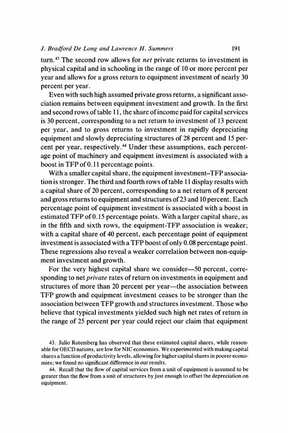
J. Bradford De Long and Lawrence H. Summers 191
turn.43 The second row allows for net private returns to investment in physical capital and in schooling in the range of 10 or more percent per year and allows for a gross return to equipment investment of nearly 30 percent per year.
Even with such high assumed private gross returns, a significant asso- ciation remains between equipment investment and growth. In the first and second rows of table 1 1, the share of income paid for capital services is 30 percent, corresponding to a net return to investment of 13 percent per year, and to gross returns to investment in rapidly depreciating equipment and slowly depreciating structures of 28 percent and 15 per- cent per year, respectively."4 Under these assumptions, each percent- age point of machinery and equipment investment is associated with a boost in TFP of 0.11 percentage points.
With a smaller capital share, the equipment investment-TFP associa- tion is stronger. The third and fourth rows of table 11 display results with a capital share of 20 percent, corresponding to a net return of 8 percent and gross returns to equipment and structures of 23 and 10 percent. Each percentage point of equipment investment is associated with a boost in estimated TFP of 0.15 percentage points. With a larger capital share, as in the fifth and sixth rows, the equipment-TFP association is weaker; with a capital share of 40 percent, each percentage point of equipment investment is associated with a TFP boost of only 0.08 percentage point. These regressions also reveal a weaker correlation between non-equip- ment investment and growth.
For the very highest capital share we consider-50 percent, corre- sponding to net private rates of return on investments in equipment and structures of more than 20 percent per year-the association between TFP growth and equipment investment ceases to be stronger than the association between TFP growth and structures investment. Those who believe that typical investments yielded such high net rates of return in the range of 25 percent per year could reject our claim that equipment
43. Julio Rotemberg has observed that these estimated capital shares, while reason- able for OECD nations, are low for NIC economies. We experimented with making capital shares a function of productivity levels, allowing for higher capital shares in poorer econo- mies; we found no significant difference in our results.
44. Recall that the flow of capital services from a unit of equipment is assumed to be greater than the flow from a unit of structures by just enough to offset the depreciation on equipment.
192 Brookings Papers on Economic Activity, 2:1992
investment is disproportionately associated with rapid TFP growth. However, they could not return to the neoclassical growth model as- sumptions that TFP is largely independent of rates of investment. In the last row of table 11, both equipment and structures investment rates are significantly associated with TFP growth.
There is no sign of any strong association between TFP growth and schooling. Changes in measured schooling do not have any strong influ- ence on the magnitude of other coefficients, and do not have a high enough partial association with output or TFP growth to suggest a social rate of return of more than 10 percent. This may well arise because our estimates of schooling are poor estimates of true investment in human capital. We interpret the (at times) negative associations of estimated TFP growth and schooling as carrying information about the inadequate nature of our proxies for educational investment, not as indicating that schooling is a relatively unproductive investment from a social stand- point.
The Social Rate of Return to Equipment Investment
In those TFP growth regressions that assume private net rates of re- turn on investments in the range that we find reasonable, a 1 percentage point increase in the equipment investment share of GDP is associated with an increase of approximately 0.10 to 0.15 percentage points per year in the TFP growth rate. Suppose that equipment investment yields a net private rate of return of 10 percent that roughly corresponds to the return on business investments, and an associated gross rate of return of 25 percent per year. What then is the social rate of return to equipment investment?
The exact calculation of the social rate of return hinges on the timing of the external rise in TFP that may be induced by equipment invest- ment. If this extra rise happens immediately-at the moment of installa- tion, as new equipment is brought on line and workers and organizations learn the skills necessary to use it efficiently-then the net social rate of return to equipment investment is 25 percent per year or so: approxi- mately 10 percent in extra privately appropriable value created through capital deepening, and approximately 15 percent through the external effects induced. Models such as that of Aghion and Howitt, in which pri- vate investment in new types of equipment raises productivity at the mo-
J. Bradford De Long and Lawrence H. Summers 193
ment of such investment, suggest such a front-loading of the TFP boost.45
If this extra rise is spread out over time proportional to the depreci- ated remaining value of the extra capital put in place, then the net social rate of return is lower because the productivity gains occur only in the future and must be discounted. In a model in which the external TFP benefits from equipment investment accrue because of learning-by-do- ing-by which, through experience, organizations and workers acquire the skills needed to handle modern technologies productively-such a time pattern would be suggested. At the 15 percent per year depreciation rate assumed for the benchmark parameters, the social rate of return is about 20 percent per year. Pushing off the external productivity benefits of investment to future years by making them proportional to current capital services substantially reduces the present value of the external productivity gains that are induced. If the external productivity gains are all delayed until the tenth year after the initial investment-an extreme assumption useful only as a bound, because by that time the depreciated value of the investment goods put in place would be only 22 percent of its initial installed value-then the net social rate of return could be as low as 15 percent per year.
Our conclusion is that cross-sectional regressions, if they will bear a causal interpretation, suggest net social rates of return from equipment investment in the range of 20 percent per year or more, under the main- tained hypothesis that the large coefficient on equipment investment arises because equipment investment is a trigger of learning-by-doing and thus of substantial total factor productivity growth. To the extent that causality flows from growth to equipment investment, as well as from investment to growth, the social rate of return would be somewhat lower. To the extent that most of the productivity gains from learning how to use and organize production with new equipment technologies would occur soon after their introduction (rather than proportionately over the lifespan of equipment), the social rate of return would be some- what higher. To be more precise would require a much sharper vision of the process of productivity growth and on-the-job-training than we possess.
45. Aghion and Howitt (1992).
194 Brookings Papers on Economic Activity, 2:1992
Conclusions and Implications
This analysis suggests a strong and causal relationship between equipment investment and economic growth. If our interpretation of the statistical data is correct, a strong case seems to exist for making sure that economic policy does not penalize, and in fact rewards, investors in equipment.
One observation, however, gives us pause. There is substantial evi- dence that the centrally planned, communist-ruled economies of the twentieth century commanded that huge fractions of GDP be devoted to machinery investment-yet these economies have not realized rapid productivity growth. If equipment investment does indeed have massive external benefits, then why didn't Stalinist Russia-which apparently invested a greater share of total output in machinery from 1929 to 1973 than Japan did from 1950 to 1973-even begin to overtake the industrial West?
We can venture an answer that attempts to resolve the apparent in- consistency between the strong cross-sectional correlation of equip- ment investment and growth in market economies and the failure of high rates of equipment investment to trigger rapid productivity growth in centrally planned economies. A given investment in equipment can yield large external benefits if learning-by-doing helps to create a work- force experienced and competent at handling modern technologies, and helps organizations to develop rules-of-thumb and standard operating procedures necessary to produce efficiently, which other firms can imi- tate. If these are the channels through which equipment investment pro- duces external benefits, then it makes sense that few such external bene- fits would be generated by investments in inappropriate technologies. No gain accrues from creating a workforce trained at technologies that subtract value. No advantage flows from the opportunity to copy the op- erating procedures of a money-losing organization. This leads us to sus- pect that the largest external benefits from equipment investment will arise from those investments that make the highest profits.
Similar reasoning might explain why some organizations that have undertaken enormous investment programs-such as General Motors (GM) in the 1980s-have reaped few productivity gains. GM invested
J. Bradford De Long and Lawrence H. Summers 195
nearly $70 billion in the 1980s in new plant and equipment. Yet as best as can be estimated, this program produced only $20 billion of wealth for shareholders and bondholders. Note that had GM not possessed the internal cash flow to finance this program, it could never have financed it through the capital markets. The high cost of external finance to GM was in large part a judgment by the market about the competence and flexibility of the organization-a conclusion demonstrated by the mar- ket's continued high valuation of other firms, such as Honda, that also have been investing in U.S. automobile manufacturing capacity.
This line of thought has a powerful implication. Economic growth is likely to be increased by policies to promote investment that conform to the market: that is, policies that alter the marginal incentives of produc- ers and investors and induce them to undertake equipment investment projects that had previously failed to meet hurdle rates. Policies that command pre-chosen, large-scale investments in equipment, whether or not they meet direct cost-benefit tests, are not likely to generate invest- ment in the kinds of equipment that generate high private benefit-cost ratios.
How best can rates of equipment investment be enhanced? First, the example of those centrally planned communist economies that at- tempted to devote enormous resources to equipment investment and yet saw few productivity gains should be heeded. That experience should lead governments to avoid nonmarket policies to boost equipment in- vestment. Even if the equipment-growth nexus is a causal one, it ap- pears to be one that is potentially swamped by the enormous inefficien- cies that command allocation processes generate. Incentives that conform to a market framework appear vastly preferable to commands that replace such a framework.
Second, governments must avoid anti-equipment incentive policies. Countries where property rights are not respected are likely to have a difficult time attracting equipment investment. Countries where macro- economic policies are unsustainable and leave the ultimate financing of current expenditures in doubt are also likely to see low rates of equip- ment investment. Large budget deficits create substantial uncertainty in future tax policies and inflation rates; to cut current taxes while increas- ing spending is not to reduce, but to randomize, tax burdens. Govern- ments that follow such cut-and-borrow policies should not be surprised
196 Brookings Papers on Economic Activity, 2:1992
when forward-looking firms and investors respond not by increasing, but by reducing, saving and investment. The best policy for the supply side is a budget surplus over the course of the business cycle.
More specific policies that discriminate against equipment include "industrial policies" that protect established firms at the expense of new entrants from home or abroad and that force purchasers to pay higher- than-world prices for the products of domestic capital goods industries. Such policies confuse a high "investment effort" with a high realized rate of investment: there is a very large difference. All over the world, gov- ernments in the post-World War II era have sought to encourage indus- trialization and growth by providing protection and subsidies for what they view as their high value-added industries. In almost every case, governments and their supporters have pointed to the limitations of laissez-faire theory and called for policies that wrench resource alloca- tion away from static "Ricardian" efficiency in the interests of attaining "Schumpeterian" efficiency.46 However, outside of East Asia, and pos- sibly Brazil, such policies appear to have been disastrous. One attrac- tive interpretation is that Pacific Rim industrial policies have managed to combine subsidization of equipment investment and exports, while maintaining a ferocious degree of domestic competition. Many indus- trial policies around the world appear to us to have confused support for modern industry with whatever enriches one's current (and vocal) popu- lation of industrialists: this seems to us another potential road to dis- aster.
Still other policies with an anti-equipment bias include tax rules that subsidize assets that can easily be levered. Because of transactions costs in second-hand markets and the dedication of equipment to partic- ular uses, pieces of equipment are frequently more difficult to use as col- lateral for debt than are investments in structures. On the labor market side, policies that make it very costly for firms to substitute capital for labor are also likely to inhibit growth by discouraging equipment invest- ment. To the extent that workers in the future will gain high wages by virtue of their skills in handling modern machine technologies, rather than by occupying niches in which quasi-rents can be captured, it is not even in labor's short-run interest to press for a reduction in the capital- labor ratio.
46. See, for example, Johnson, Tyson, and Zysman (1989).
J. Bradford De Long and Lawrence H. Summers 197
Third, governments can promote equipment investment in a number of ways. Given that international capital markets remain imperfectly in- tegrated, increases in national saving-whether induced by deficit re- duction or by policies that increase private saving-translate into some increased equipment investment. Those who believe that international capital markets will not channel substantial long-run flows see an extra 35 cents of equipment coming from each dollar of deficit reduction or increased private savings. Those who believe in open capital markets would divide that estimate by two or three.
Measures that reduce the tax burden on new equipment investments are likely to be especially potent in maximizing the equipment invest- ment engendered per dollar of government revenue forgone. While we have little confidence in any of the formal quantitative estimates, we think that each dollar of revenue lost from an equipment investment tax credit would generate an extra dollar of equipment investment-with a larger benefit-cost ratio for an incremental investment tax credit.47
These policy implications regarding equipment investment have par- ticular resonance for the United States today, especially in terms of its performance relative to the benchmarks set by other industrial econo- mies, such as Germany and Japan. That the United States, with a low net saving rate relative to other advanced industrial economies, has seen its national saving rate dip further in the 1980s is well known: in the 1980s, the net national saving rate-3 percent-has been less than two- fifths its value in the 1960s and 1970s. The decline in investment was par- tially cushioned by the large borrowings from abroad of the mid- 1980s, but the capital inflow has been substantially reduced in the last half dec- ade. Since the mid-1980s, largely because of fiscal mismanagement, in- vestment in the United States as a share of national product has fallen to levels that have not been seen since the Great Depression.
If past equipment investment contributes over time to TFP growth, then the United States' relatively poor past performance may have al- ready hindered the country's ability to catch up to and match the TFP growth performance of economies such as Japan. Figure 7 plots the equipment capital stock per worker level in Japan and in the United States during the 1980s. The figure shows a large and growing gap that
47. They will, however, change the mix of investment toward equipment, which may have substantial benefits.
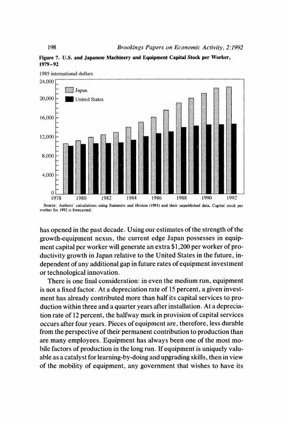
198 Brookings Papers on Economic Activity, 2:1992
Figure 7. U.S. and Japanese Machinery and Equipment Capital Stock per Worker, 1979-92
1985 international dollars
24,000
LE Japan 20,000 - United States l
_ m 1 M.81 sA.>- ...~~~~~~~~~~~~~~~~~~~~... ..... 16,000 -
12,000 -
8,000
4,000 -
0 1978 1980 1982 1984 1986 1988 1990 1992
Source: Authors' calculations using Summers and Heston (1991) and their unpublished data. Capital stock per worker for 1992 is forecasted.
has opened in the past decade. Using our estimates of the strength of the growth-equipment nexus, the current edge Japan possesses in equip- ment capital per worker will generate an extra $1,200 per worker of pro- ductivity growth in Japan relative to the United States in the future, in- dependent of any additional gap in future rates of equipment investment or technological innovation.
There is one final consideration: in even the medium run, equipment is not a fixed factor. At a depreciation rate of 15 percent, a given invest- ment has already contributed more than half its capital services to pro- duction within three and a quarter years after installation. At a deprecia- tion rate of 12 percent, the halfway mark in provision of capital services occurs after four years. Pieces of equipment are, therefore, less durable from the perspective of their permanent contribution to production than are many employees. Equipment has always been one of the most mo- bile factors of production in the long run. If equipment is uniquely valu- able as a catalyst for learning-by-doing and upgrading skills, then in view of the mobility of equipment, any government that wishes to have its

J. Bradford De Long and Lawrence H. Summers 199
economy grow rapidly must take extraordinary pains to make sure that investors in equipment see the economy as a hospitable environment. Ample provision of infrastructure; a skilled, trained, and motivated workforce; and low taxes on new capital investments may well pay for themselves (because we live in a world where equipment investments are mobile) by virtue of the extra equipment investment they induce.
Comments and Discussion
Andrew B. Abel: This paper is an important extension of the paper by Bradford De Long and Lawrence Summers published in the May 1991 Quarterly Journal of Economics (QJE). The QJE paper documented a statistically significant and robust cross-country partial correlation be- tween the growth rate of GDP per worker and the equipment invest- ment/GDP ratio. The current paper extends the sample in both the time dimension and the cross-section dimension and finds the same result: when various factors are held constant, a 1 percentage point increase in the equipment investment/GDP ratio is associated with an increase of about 0.20 to 0.35 percentage points in the growth rate of GDP per worker. Of course, allowing for sampling error, the range is probably somewhat wider. In both investigations, De Long and Summers went to great lengths to make this finding go away, but the finding survived fairly intense scrutiny. It is only slightly, if at all, premature, to say that De Long and Summers have presented us with a new stylized fact. Not only does the new stylized fact appear to be a "true" fact, but it is an interest- ing fact because it is apparently not readily explained within the stan- dard growth theoretic framework.
In my comments, I will accept the new stylized fact as a fact and I will focus on the interpretation of the partial correlation uncovered by De Long and Summers. The authors argue that if productivity growth is in- dependent of factor accumulation, then the standard growth accounting framework can account for a coefficient of only about 0.08 in a cross- sectional regression of growth rates on equipment investment/GDP ra- tios over a 25-year horizon. Because a typical value of the coefficient estimated by De Long and Summers is about 0.25, they argue that there is a gap of 0.17 to be explained by externalities. The report's discussion of the role of new equipment in providing an opportunity for learning-
200
J. Bradford De Long and Lawrence H. Summers 201
by-doing seems compelling; at an intuitive level, I find this mechanism to be an attractive explanation of at least some of the growth process. However, before abandoning the standard growth theoretic framework, which does not appeal to externalities, I need to be more convinced that the new stylized fact is inconsistent with the standard framework.
My lingering doubt concerns the statement that the standard growth accounting framework predicts a coefficient of only about 0.08 in a re- gression of growth rates on equipment investment/GDP ratios. The value of this coefficient is very sensitive to the timing of changes in the equipment investment/GDP ratio over a 25-year horizon. To illustrate this sensitivity, consider the following simple model. Output in year t, Y(t), is produced according to the Cobb-Douglas production function
(1) Y(t) = KE(t)t Ks(t) L(t)I --,
where KE(t) is the stock of equipment at the beginning of year t, KS(t) is the stock of structures at the beginning of year t, and L(t) is the amount of effective units labor in year t. Along the initial steady-state growth path, there is no embodied technical progress for equipment or struc- tures. The effective units of labor grow according to L(t) = (1 + n)(1 + g) L(t - 1), where n is the population growth rate and g is the growth of effective units of labor per worker. Let iE(t) be the equipment invest- ment/output ratio and let is(t) be the structures investment/output ratio. In the initial steady state, with both types of capital growing at the rate (n + g), the capital equipment/output ratio is iE'[(l + n)(1 + g) - (1 - dE)], where dE is the depreciation rate of equipment. The capital structures/ output ratio is isl[(I + n)(1 + g) - (1 - ds)], where ds is the depreciation rate of structures.
Now consider starting from the initial steady state and increasing the average equipment investment/output ratio by 1 percentage point over a 25-year horizon. Based on an earlier draft of the report, set iE equal to 0.075, is equal to 0.100, dE equal to 0.17, and ds equal to 0.02. In addition, set n equal to 0.01 and g equal to 0.02 so that (n + g) equals 0.03. Finally, set a equal to 0.10 and 3 equal to 0.15. With these parameter values, the net marginal product of equipment is 9.7 percent, which is about the same as the 9.5 percent net marginal product of structures.
Now consider a permanent increase in iE(t) to a value of 0.085. As a result of this increase in equipment investment, the average growth rate of output over the subsequent 25 years increases by 0.063 percent,

202 Brookings Papers on Economic Activity, 2:1992
which yields a coefficient of output growth on iE of 0.063-close to the value of 0.08 found by De Long and Summers using different (implied) values of a and P.
But what would the regression coefficient be if instead of jumping to 0.085, iE rose linearly over a 25-year horizon and the average over this horizon was 0.085? In this case, the coefficient increases to 0.092. The later during the 25-year horizon that the increase in iE(t) occurs, the larger will be the regression coefficient of growth on iE. For instance, if iE(t) remains 0.075 for 15 years and then increases to 0.100 for 10 years, the average value of iE will rise by 1 percentage point to 0.085, but the regression coefficient would be 0.119. If the increase in iE(t) is concen- trated in the last five years of the horizon, the regression coefficient in- creases to 0.161.
Is the timing of iE(t) that yields a regression coefficient of 0.161 realis- tic? I do not honestly know, but I would not be shocked to learn that the countries with high average values of iE from 1960 to 1985 were the countries that took advantage of the computer revolution and substan- tially increased their equipment investment in the 1980s.
The calculations presented above were calculated under the assump- tion-imposed by De Long and Summers when computing standard growth theoretic predictions of the regression coefficient-that produc- tivity growth is independent of factor accumulation. But why did differ- ent countries invest different shares of GDP in equipment? De Long and Summers use data on the relative price of equipment to argue-convinc- ingly, in my opinion-that high rates of equipment investment were driven by rightward shifts of the supply curve for equipment, rather than by rightward shifts of the demand curve for equipment. As they point out, a predominance of supply shifts would account for the observed negative cross-sectional correlation between equipment investment and the relative price of equipment.
One possible source of rightward shifts of the equipment supply curve is technical progress in equipment, which reduces the price of an effective unit of equipment. Put differently, those countries in which the level of technology embodied in equipment grew rapidly and was ex- pected to grow rapidly would be attractive environments for equipment investment. If a high rate of equipment investment resulted from rapid technological progress embodied in equipment, then the standard growth accounting framework would attribute output growth both to the
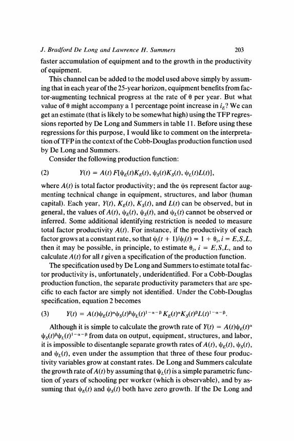
J. Bradford De Long and Lawrence H. Summers 203
faster accumulation of equipment and to the growth in the productivity of equipment.
This channel can be added to the model used above simply by assum- ing that in each year of the 25-year horizon, equipment benefits from fac- tor-augmenting technical progress at the rate of 0 per year. But what value of 0 might accompany a 1 percentage point increase in iE? We can get an estimate (that is likely to be somewhat high) using the TFP regres- sions reported by De Long and Summers in table 11. Before using these regressions for this purpose, I would like to comment on the interpreta- tion of TFP in the context of the Cobb-Douglas production function used by De Long and Summers.
Consider the following production function:
(2) Y(t) = A(t) F[4E(t)KE(t), S(t)KS(t), L(t)L(t)],
where A(t) is total factor productivity; and the 4s represent factor aug- menting technical change in equipment, structures, and labor (human capital). Each year, Y(t), KE(t), KS(t), and L(t) can be observed, but in general, the values of A(t), E(t), 4s(t), and L(t) cannot be observed or inferred. Some additional identifying restriction is needed to measure total factor productivity A(t). For instance, if the productivity of each factor grows at a constant rate, so that i(t + 1)A*i(t) = 1 + Oi, i = E,S,L, then it may be possible, in principle, to estimate Oi, i = E,S,L, and to calculate A(t) for all t given a specification of the production function.
The specification used by De Long and Summers to estimate total fac- tor productivity is, unfortunately, underidentified. For a Cobb-Douglas production function, the separate productivity parameters that are spe- cific to each factor are simply not identified. Under the Cobb-Douglas specification, equation 2 becomes
(3) Y(t) = A(t)4E(t)o4fS(t)'3L(t)' - '-KE(t)OKs(t)'L(t)I - '3-
Although it is simple to calculate the growth rate of Y(t) = A(t)0E(t)P
S(t)0P*L(t)1'- from data on output, equipment, structures, and labor, it is impossible to disentangle separate growth rates of A(t), E(t), S(t),
and L(t), even under the assumption that three of these four produc- tivity variables grow at constant rates. De Long and Summers calculate the growth rate of A(t) by assuming that L(t) is a simple parametric func- tion of years of schooling per worker (which is observable), and by as- suming that E(t) and 4s(t) both have zero growth. If the De Long and
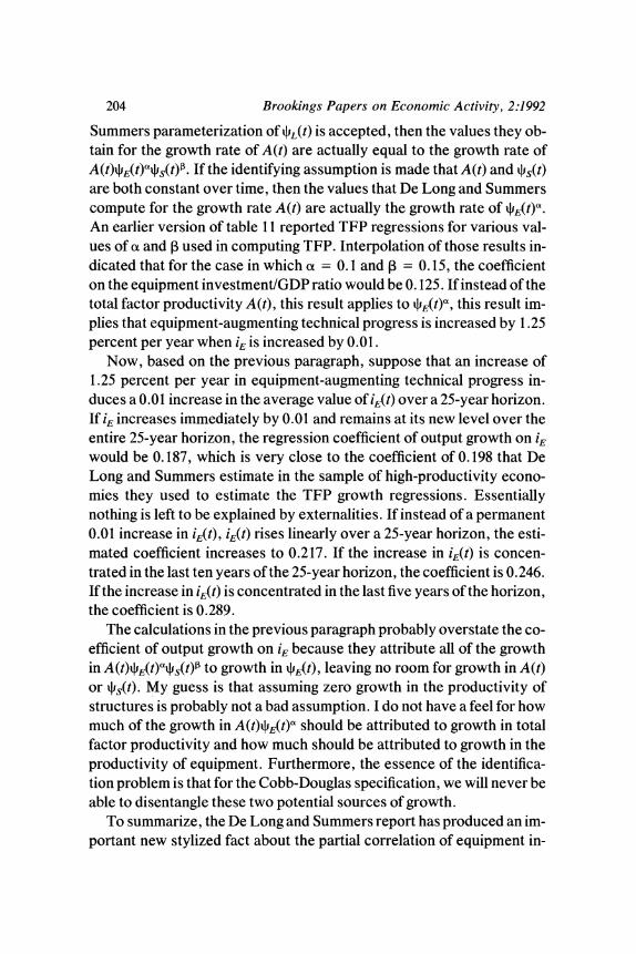
204 Brookings Papers on Economic Activity, 2:1992
Summers parameterization of L(t) is accepted, then the values they ob- tain for the growth rate of A(t) are actually equal to the growth rate of A(t)4E(t)bIS(t)'. If the identifying assumption is made that A(t) and 4s(t) are both constant over time, then the values that De Long and Summers compute for the growth rate A(t) are actually the growth rate of 4E(t)O.
An earlier version of table 11 reported TFP regressions for various val- ues of a and P. used in computing TFP. Interpolation of those results in- dicated that for the case in which a = 0.1 and 1P = 0.15, the coefficient on the equipment investment/GDP ratio would be 0.125. If instead of the total factor productivity A(t), this result applies to E(t)0, this result im- plies that equipment-augmenting technical progress is increased by 1.25 percent per year when iE is increased by 0.01.
Now, based on the previous paragraph, suppose that an increase of 1.25 percent per year in equipment-augmenting technical progress in- duces a 0.01 increase in the average value of iE(t) over a 25-year horizon. If iE increases immediately by 0.01 and remains at its new level over the entire 25-year horizon, the regression coefficient of output growth on iE
would be 0.187, which is very close to the coefficient of 0.198 that De Long and Summers estimate in the sample of high-productivity econo- mies they used to estimate the TFP growth regressions. Essentially nothing is left to be explained by externalities. If instead of a permanent 0.01 increase in iE(t), iE(t) rises linearly over a 25-year horizon, the esti- mated coefficient increases to 0.217. If the increase in iE(t) is concen- trated in the last ten years of the 25-year horizon, the coefficient is 0.246. If the increase in iE(t) is concentrated in the last five years of the horizon, the coefficient is 0.289.
The calculations in the previous paragraph probably overstate the co- efficient of output growth on iE because they attribute all of the growth in A(t)*E(t)OiPS(t) to growth in E(t), leaving no room for growth in A(t) or 4s(t). My guess is that assuming zero growth in the productivity of structures is probably not a bad assumption. I do not have a feel for how much of the growth in A(t)PE(t)x should be attributed to growth in total factor productivity and how much should be attributed to growth in the productivity of equipment. Furthermore, the essence of the identifica- tion problem is that for the Cobb-Douglas specification, we will never be able to disentangle these two potential sources of growth.
To summarize, the De Long and Summers report has produced an im- portant new stylized fact about the partial correlation of equipment in-
J. Bradford De Long and Lawrence H. Summers 205
vestment and output growth. My discussion has not focused on the va- lidity of this fact because this report and the QJE paper together virtually convince me that it is true. I also find attractive the explanations of this stylized fact that involve externalities and learning-by-doing. But my re- luctance to completely embrace these explanations is perhaps best ex- pressed in the language of hypothesis testing. The null hypothesis is some version of standard growth theory without externalities, and the alternative hypothesis is that externalities are important in the growth process. In my discussion, I have attempted to show that the stylized fact is not inconsistent with the null hypothesis, which means that it is premature to reject the null hypothesis of no externalities. As in any hy- pothesis testing, failure to reject the null hypothesis is not the same as accepting the null hypothesis. De Long and Summers have offered a credible alternative hypothesis; future work may actually lead to a con- vincing rejection of the null hypothesis in favor of their alternative. But for now, there does not seem to be enough evidence to throw away the null hypothesis.
General Discussion
Robert Gordon questioned the paper's implication that an investment tax credit for equipment would be preferable to greater funding of educa- tion or public infrastructure. He pointed out that, since the 1930s, the ratio of equipment to structures in the United States has increased sharply, with a significant decline in the average productivity of U.S. equipment, suggesting a decline in its marginal productivity as well. He reported calculations of marginal factor productivity growth using dif- ferent assumptions about capital. Attributing the entire share of capital to equipment, he found zero marginal productivity growth for equip- ment since 1964. With various other assumptions, productivity growth has slowed in recent years. Gordon questioned whether the cross-sec- tional findings in the paper could be reconciled with this U.S. time-series experience.
Echoing Bill Clinton's campaign slogan, Summers responded that he, too, believed in "putting people first." Investments in human capital and good infrastructure are not only desirable in their own right, but are needed to improve the productivity of equipment. He acknowledged
206 Brookings Papers on Economic Activity, 2:1992
the contradiction between U.S. time-series evidence and the cross- sectional evidence in the paper, but argued that the cross-sectional evidence was the more persuasive. He suggested as a corollary of the report's results that the welfare loss caused by distortions in the cost of capital through investment tax incentives is very small, relative to their effects on growth.
Most panel members accepted the paper's new "stylized fact" that equipment investment had a higher-than-expected effect on output growth. However, Mancur Olson questioned whether the association is causal. He suggested that higher equipment investment may simply be associated with other growth-inducing factors. Because all countries have the same access to equipment at similar prices (excluding transport costs), differences in economic performance cannot be fully explained by equipment investment alone. There must be a reason why some countries invest in more or less equipment than others, and whatever those reasons are, they themselves may be the reasons for differences in growth. He noted, for example, that Argentina, with terrible general economic policy, had low growth and, perhaps only incidentally, had low investment in equipment. In the same vein, Robert Hall suggested that policies that encouraged investment in equipment are often part of a package of standard free-market economic policies. Equipment in- vestment is therefore a proxy for the pro-trade and pro-growth policies that in fact are responsible for high growth.
Summers defended the claim that the equipment variable is not sim- ply a proxy for other policies. First, he noted that instrumenting for changes in equipment investment with a variable that is not strongly cor- related with other policies-changes in the saving rate-does not alter the results. Second, the effect of equipment remained when the authors included other variables that attempt to directly capture the broad policy regime, such as the World Bank index of openness. Third, if the extent of liberalization were driving the results, then, when both quantity and price in the regressions are included, it would be expected that the price variable would be significant. This relationship would be predicted be- cause equipment prices reflect tariff barriers and other internal distor- tions. In fact, only the quantity variable remains significant in this form of regression.
William Nordhaus was not convinced that the instruments used were uncorrelated with other variables in the regression. He proposed using
J. Bradford De Long and Lawrence H. Summers 207
genuinely exogenous variables such as the investment tax credit or the depreciation allowance, which changed frequently in countries such as the United Kingdom. Summers replied that he and De Long were not convinced that looking at year-to-year variations in such instruments would be a way of testing for externalities. In addition, the investment incentives are not fully exogenous because governments often intro- duce them when investment is low. He reported that he and De Long searched unsuccessfully for sufficient data on effective tax rates on equipment.
Christopher Sims pointed out that the policy implications of the paper would be different if one did not accept its conclusion that the observed statistical association of equipment investment share with growth must reflect an externality. He did not doubt the statistical association, but saw three main reasons to be skeptical of its representing an externality.
First, the paper's theoretical calculations that show weak associa- tions of equipment investment share with growth rates in a model with- out externalities are undertaken as though variations in investment share were sustained over the 15-to-40 year periods considered. The re- gression results apply to growth rates over historical 15-year periods in which shares of investment were not constant within each country. Even the very long-run panel, although it uses data from a long span of time, uses 15-year averages as data points. If there were any substantial fluctuation in investment shares over time within these 15-year periods, the relevant T in table 10 might well be closer to 5 or 7 than to 15.
Second, embodiment effects (which make productivity on newly in- stalled equipment higher than on old equipment and may cause obsolete equipment to be retired before it has physically decayed) would make intermediate-run elasticities of productivity with respect to gross invest- ment substantially higher than long-run elasticities-and by more than would be implied by table 10, without this implying any externality.
Finally, the paper's arguments for a structural interpretation for its regression have weaknesses. If there were little room for substitution between equipment and other factors, so that technology required a nearly fixed ratio of output to equipment stock, then the bivariate rela- tionship of investment share to output growth rate would be nearly pro- portional. To capture correctly from data the fact that investment share increases nonetheless have small effects (if other factors are held con- stant), we would have to account completely and accurately for these
208 Brookings Papers on Economic Activity, 2:1992
other factors in the regression specification. To the extent that we do not have data on these factors, they would enter the error term, and the as- sumed lack of substitutability would imply that they are strongly corre- lated with the equipment investment share regressor. The paper uses in- struments that are plausibly correlated with equipment investment but not with, say, an exogenous disturbance to the level of technical knowl- edge. But if the disturbances in these regressions come from omitted fac- tors of production that, because of the technology, must respond almost automatically to increases in output and equipment, the instruments used in the paper will do little to reduce the simultaneity bias.
If the vintage model of equipment is correct, Sims reasoned that cal- culations of social return on equipment for periods of time like those used in the paper would be greatly affected. He carried his argument to the cases of Argentina and Japan discussed in the paper: Argentine poli- cies toward equipment may indeed have kept output below the tech- nological frontier, and hence retarded growth. By contrast, Japanese investment policies may have led to wastefully high obsolescence rates, stimulating productivity at too high a cost in forgone consumption. Joseph Stiglitz agreed that it would be desirable to take into account vin- tage effects, but noted that equipment is short-lived in practice. There- fore, although a model assuming embodiment may give an initial spurt in growth, he doubted that it would be significant over the time period considered in the report.
Summers acknowledged the need for more work on the issue of em- bodiment and the need to distinguish between the social return on equip- ment investment and external returns associated with equipment. How- ever, he believed that the increase in output associated with equipment investment over a 25-year period cannot be explained without externali- ties, unless private returns are on the order of 20 to 25 percent per year.
Others questioned whether learning-by-doing is the source of the ex- ternality as suggested by the paper. Nordhaus remarked that the case of the Swedish Horndal plant, which had inspired the Arrow model of learning-by-doing, does not fit the externality story because the produc- tivity increase seemed unrelated to investment. He agreed that the rates of return on different kinds of investment may be unequal, citing the ex- ample .of energy conservation projects in California, where there is evi- dence of extremely high private and social rates of return. Stiglitz of- fered another mechanism by which equipment investment could have
J. Bradford De Long and Lawrence H. Summers 209
large social returns. He suggested that equipment investment may be closely associated with the use of nontraded intermediate goods, whose production involves high fixed costs. Hence greater equipment invest- ment stimulates demand for intermediate goods, which have a lower cost when produced in larger volumes. This induced scale economy can be thought of as a positive externality of the equipment investment.
Julio Rotemberg called attention to the use of OECD shares of labor and capital in the production function. The share of capital is typically much higher in developing countries than in the OECD, leading to the association of high growth rates and high capital shares in standard models. He noted that the current model would indicate high TFP growth for Singapore, although other studies have found no TFP growth at all. The latter result is caused by Singapore's output growth being lower than expected from its very high investment rate. This prompted Gordon to suggest adding Singapore to the two "S's" described in the paper-Josef Stalin and former General Motors chairman Roger Smith-as cases in which rapid growth in equipment investment did not lead to correspondingly rapid output growth. Stiglitz remarked that cal- culations of TFP in countries such as Singapore are problematic: not only are factor prices noncompetitive because of government controls, but state-owned firms, which are major investors, do not necessarily op- timize in the neoclassical sense. As a result, the production function co- efficients assumed for such countries may be meaningless.
Martin Weitzman questioned the application of the conventional de- mand-and-supply apparatus to the equipment market and was therefore skeptical that the observed price-quantity correlations could be used to establish the direction of causation. Weitzman argued that the market structure for equipment is either oligopolistic or monopolistically com- petitive; thus high quantities may be associated with low prices, not necessarily with high prices, as the perfectly competitive model pre- dicts. Gregory Mankiw added that the equipment prices used in the pa- per might simply reflect the relative price of traded versus nontraded goods. In this case, rapid economic growth would lead to higher prices of nontraded goods, resulting in the lower price ratio observed. Thus the association of lower relative prices and higher quantities does not neces- sarily establish the supply-side causation that the report argues.
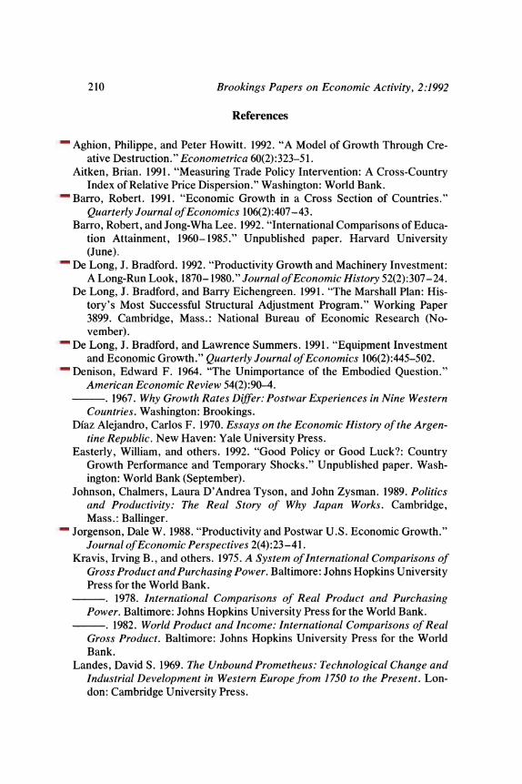
210 Brookings Papers on Economic Activity, 2:1992
References
Aghion, Philippe, and Peter Howitt. 1992. "A Model of Growth Through Cre- ative Destruction." Econometrica 60(2):323-51.
Aitken, Brian. 1991. "Measuring Trade Policy Intervention: A Cross-Country Index of Relative Price Dispersion." Washington: World Bank.
Barro, Robert. 1991. "Economic Growth in a Cross Section of Countries." Quarterly Journal of Economics 106(2):407-43.
Barro, Robert, and Jong-Wha Lee. 1992. "International Comparisons of Educa- tion Attainment, 1960-1985." Unpublished paper. Harvard University (June).
De Long, J. Bradford. 1992. "Productivity Growth and Machinery Investment: A Long-Run Look, 1870-1980." Journal of Economic History 52(2):307-24.
De Long, J. Bradford, and Barry Eichengreen. 1991. "The Marshall Plan: His- tory's Most Successful Structural Adjustment Program." Working Paper 3899. Cambridge, Mass.: National Bureau of Economic Research (No- vember).
De Long, J. Bradford, and Lawrence Summers. 1991. "Equipment Investment and Economic Growth." Quarterly Journal of Economics 106(2):445-502.
Denison, Edward F. 1964. "The Unimportance of the Embodied Question." American Economic Review 54(2):90-4.
. 1967. Why Growth Rates Differ: Postwar Experiences in Nine Western Countries. Washington: Brookings.
Diaz Alejandro, Carlos F. 1970. Essays on the Economic History of the Argen- tine Republic. New Haven: Yale University Press.
Easterly, William, and others. 1992. "Good Policy or Good Luck?: Country Growth Performance and Temporary Shocks." Unpublished paper. Wash- ington: World Bank (September).
Johnson, Chalmers, Laura D'Andrea Tyson, and John Zysman. 1989. Politics and Productivity: The Real Story of Why Japan Works. Cambridge, Mass.: Ballinger.
Jorgenson, Dale W. 1988. "Productivity and Postwar U.S. Economic Growth." Journal of Economic Perspectives 2(4):23-41.
Kravis, Irving B., and others. 1975. A System of International Comparisons of Gross Product and Purchasing Power. Baltimore: Johns Hopkins University Press for the World Bank.
1978. International Comparisons of Real Product and Purchasing Power. Baltimore: Johns Hopkins University Press for the World Bank.
. 1982. World Product and Income: International Comparisons of Real Gross Product. Baltimore: Johns Hopkins University Press for the World Bank.
Landes, David S. 1969. The Unbound Prometheus: Technological Change and Industrial Development in Western Europe from 1750 to the Present. Lon- don: Cambridge University Press.
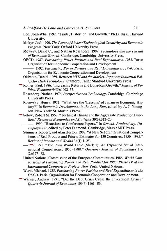
J. Bradford De Long and Lawrence H. Summers 211
Lee, Jong-Wha. 1992. "Trade, Distortion, and Growth." Ph.D. diss., Harvard University.
Mokyr, Joel. 1990. The Lever of Riches: Technological Creativity and Economic Progress. New York: Oxford University Press.
Mowery, David C., and Nathan Rosenberg. 1989. Technology and the Pursuit of Economic Growth. Cambridge: Cambridge University Press.
OECD. 1987. Purchasing Power Parities and Real Expenditures, 1985. Paris: Organisation for Economic Cooperation and Development.
. 1992. Purchasing Power Parities and Real Expenditures, 1990. Paris: Organisation for Economic Cooperation and Development.
Okimoto, Daniel. 1989. Between MITI and the Market: Japanese Industrial Pol- icy for High Technology. Stanford, Calif.: Stanford University Press.
Romer, Paul. 1986. "Increasing Returns and Long-Run Growth. " Journal of Po- litical Economy 94(5): 1002-37.
Rosenberg, Nathan. 1976. Perspectives on Technology. Cambridge: Cambridge University Press.
Rosovsky, Henry. 1972. "What Are the 'Lessons' of Japanese Economic His- tory?" In Economic Development in the Long Run, edited by A. J. Young- son. New York: St. Martin's Press.
Solow, Robert M. 1957. "Technical Change and the Aggregate Production Func- tion." Review of Economics and Statistics 39(3):312-20.
. 1990. "Reactions to Conference Papers." In Growth, Productivity, Un- employment, edited by Peter Diamond. Cambridge, Mass.: MIT Press.
Summers, Robert, and Alan Heston. 1988. "A New Set of International Compar- isons of Real Product and Prices: Estimates for 130 Countries, 1950-1985." Review ofIncome and Wealth 34(1):1-25.
. 1991. "The Penn World Table (Mark 5): An Expanded Set of Inter- national Comparisons, 1950-1988." Quarterly Journal of Economics 106 (2):327-68.
United Nations, Commission of the European Communities. 1986. World Com- parisons of Purchasing Power and Real Product for 1980: Phase IV of the International Comparison Project. New York: United Nations.
Ward, Michael. 1985. Purchasing Power Parities and Real Expenditures in the OECD. Paris: Organisation for Economic Cooperation and Development.
Warner, Andrew. 1991. "Did the Debt Crisis Cause the Investment Crisis?" Quarterly Journal of Economics 107(4): 1161-86.