epic status of calibration and data analysis

XMM-Newton Calibration Technical Note

XMM-SOC-CAL-TN-0018

EPIC Status of Calibration and Data Analysis

Edited by M.J.S. Smith (ESAC)on behalf of the EPIC Consortium

December 12, 2016

History

Version Date Editor Note

3.8 December 12, 2016 Michael Smith Aligned to SASv15.0 and SASv16.0; updated URLs3.7 September 10, 2015 Michael Smith Aligned to SASv14.03.6 September 1, 2014 Matteo Guainazzi Revision by the XMM-Newton Project Scientist3.5 August 8, 2014 Matteo Guainazzi Revision by the XMM-Newton Science Support Manager3.4 August 8, 2014 Matteo Guainazzi Aligned to SASv13.5

Fig. 1 (ELLBETA calibration accuracy)Fig. 2 (Relative area calibration accuracy)

3.3 October 2, 2013 Matteo Guainazzi Sect. 6 aligned to XMM-CCF-REL-300Possible contamination in the MOS cameras (Sect. 2.3)

3.2 August 25, 2013 Matteo Guainazzi Aligned to SASv13 (see Sect. 12 for a list of changes)3.1 July 24, 2012 Matteo Guainazzi Aligned to SASv123.0 November 16, 2011 Matteo Guainazzi First LATEX version (from Version 2.13)

1

XMM-Newton Technical Note XMM-SOC-CAL-TN-0018 Page: 2

Contents

1 Scope 4

2 Calibration Overview 4

2.1 Summary . . . . . . . . . . . . . . . . . . . . . . . . . . . . . . . . . . . . . . . . . . 4

2.2 Summary of Important Improvements Since the Previous Issue . . . . . . . . . . . . 4

2.3 Summary of Important Ongoing Calibration Topics . . . . . . . . . . . . . . . . . . . 5

3 Imaging 6

3.1 Astrometry . . . . . . . . . . . . . . . . . . . . . . . . . . . . . . . . . . . . . . . . . 6

3.2 Point Spread Function and Encircled Energy . . . . . . . . . . . . . . . . . . . . . . 7

4 Effective Area 9

4.1 Mirror Collecting Area . . . . . . . . . . . . . . . . . . . . . . . . . . . . . . . . . . . 9

4.2 Filter Transmission . . . . . . . . . . . . . . . . . . . . . . . . . . . . . . . . . . . . . 10

4.3 CCD Quantum Efficiency . . . . . . . . . . . . . . . . . . . . . . . . . . . . . . . . . 10

4.4 EPIC-MOS Contamination . . . . . . . . . . . . . . . . . . . . . . . . . . . . . . . . 12

4.5 Vignetting . . . . . . . . . . . . . . . . . . . . . . . . . . . . . . . . . . . . . . . . . . 12

5 Energy Redistribution 13

5.1 EPIC-MOS . . . . . . . . . . . . . . . . . . . . . . . . . . . . . . . . . . . . . . . . . 13

5.2 EPIC-pn . . . . . . . . . . . . . . . . . . . . . . . . . . . . . . . . . . . . . . . . . . . 14

6 CTI and Gain 15

7 Background 16

8 Timing 19


9 Cross Calibration 22

10 Unexpected Events 22

10.1 Micrometeoroid Impacts . . . . . . . . . . . . . . . . . . . . . . . . . . . . . . . . . . 22

11 Data Analysis 24

11.1 New Features in SAS . . . . . . . . . . . . . . . . . . . . . . . . . . . . . . . . . . . . 24

11.1.1 SASv16.0 . . . . . . . . . . . . . . . . . . . . . . . . . . . . . . . . . . . . . . 24

11.1.2 SASv15.0 . . . . . . . . . . . . . . . . . . . . . . . . . . . . . . . . . . . . . . 24

11.1.3 SASv14.0 . . . . . . . . . . . . . . . . . . . . . . . . . . . . . . . . . . . . . . 24

11.1.4 SASv13.5 . . . . . . . . . . . . . . . . . . . . . . . . . . . . . . . . . . . . . . 25

11.1.5 SASv13.0 . . . . . . . . . . . . . . . . . . . . . . . . . . . . . . . . . . . . . . 25

11.1.6 SASv12.0 . . . . . . . . . . . . . . . . . . . . . . . . . . . . . . . . . . . . . . 25

11.1.7 SASv11.0 . . . . . . . . . . . . . . . . . . . . . . . . . . . . . . . . . . . . . . 25

11.1.8 SASv10.0 . . . . . . . . . . . . . . . . . . . . . . . . . . . . . . . . . . . . . . 25

11.1.9 SASv9.0 . . . . . . . . . . . . . . . . . . . . . . . . . . . . . . . . . . . . . . . 25

11.1.10 SASv8.0 . . . . . . . . . . . . . . . . . . . . . . . . . . . . . . . . . . . . . . . 26

11.1.11 SASv7.1 . . . . . . . . . . . . . . . . . . . . . . . . . . . . . . . . . . . . . . . 26

11.1.12 SASv7.0 . . . . . . . . . . . . . . . . . . . . . . . . . . . . . . . . . . . . . . . 26

11.1.13 SASv6.5 . . . . . . . . . . . . . . . . . . . . . . . . . . . . . . . . . . . . . . . 26

11.2 Data Analysis . . . . . . . . . . . . . . . . . . . . . . . . . . . . . . . . . . . . . . . . 27

11.2.1 EPIC-MOS . . . . . . . . . . . . . . . . . . . . . . . . . . . . . . . . . . . . . 27

11.2.2 EPIC-pn . . . . . . . . . . . . . . . . . . . . . . . . . . . . . . . . . . . . . . 28

11.2.3 Counting Mode . . . . . . . . . . . . . . . . . . . . . . . . . . . . . . . . . . . 30

12 History of This Document 30


1 Scope

This document reflects the status of the calibration of the EPIC camera as implemented in SASv16.0with the set of calibration files (Current Calibration Files, CCFs) available at the date of thedocument, unless otherwise specified. Furthermore, the outlook is considered for improvements ofcalibration, which at the moment can be expected for the next SAS release.

2 Calibration Overview

This section gives a short overview of the status of the calibration of the EPIC instruments MOS1,MOS2 and pn, operating on-board the XMM-Newton observatory. It summarises the qualityof the calibration to the extent that this may influence the scientific interpretation of the re-sults. The instrument calibration is based on a combination of physical and empirical modelsof the various components including mirror response, filter transmission and detector response(energy redistribution, charge transfer efficiency (CTE), gain). During ground calibration vari-ous components were calibrated and the model for each component was optimised. These mod-els were verified in flight and are, where relevant, continuously monitored (e.g. contaminationof the detector, changes in gain and CTE due to effects of radiation). Corrections, which areneeded for these time-variable changes, will be applied to the Current Calibration Files and/orthe processing software. For more detailed information see the release notes of the CCFs at:http://www.cosmos.esa.int/web/xmm-newton/ccf-release-notes. A general description of theinstruments, as well as preliminary calibration results, were published by Turner et al. (2001, A&A,365. L27; EPIC-MOS) and Struder et al. (2001, A&A, 365, 18; EPIC-pn).

2.1 Summary

Tab. 1 shows a summary of the status of the calibration for sources at the nominal boresight position(“on-axis”).

2.2 Summary of Important Improvements Since the Previous Issue

• Astrometry correction: An inconsistent definition of a boresight angle has been corrected(Saxton, 2016, XMM-CCF-REL-3321). This is explained in more detail in Sect. 3.1.

• Slew-specific parameterisation of the EPIC-pn PSF: A PSF for slew sources has beenintroduced. This has been calculated by averaging point source PSFs over a range of off-axisangles (Read et al., 2016, XMM-CCF-REL-3332).

• Modified EPIC-pn pattern fraction model: Following the implementation of the empir-ical doubles event energy correction in SASv14, the singles and doubles event pattern fraction

1http://xmm2.esac.esa.int/docs/documents/CAL-SRN-0332-1-0.ps.gz2http://xmm2.esac.esa.int/docs/documents/CAL-SRN-0333-1-0.ps.gz


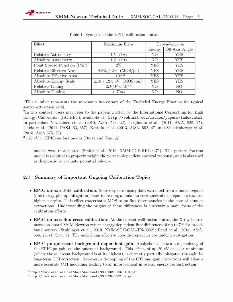
Table 1: Synopsis of the EPIC calibration status

Effect Maximum Error Dependency onEnergy Off-Axis Angle

Relative Astrometry 1.5” (1σ) NO YES

Absolute Astrometry 1.2” (1σ) NO YES

Point Spread Function (PSF)1 2% YES YES

Relative Effective Area ±3% / 2% (MOS/pn) YES YES

Absolute Effective Area ±10%2 YES YES

Absolute Energy Scale ±10 / 12.5 eV (MOS/pn)3 YES YES

Relative Timing ∆P/P < 10−8 NO NO

Absolute Timing < 70µs NO NO

1This number represents the maximum inaccuracy of the Encircled Energy Fraction for typicalsource extraction radii.2In this context, users may refer to the papers written by the International Consortium for HighEnergy Calibration (IACHEC), available at: http://web.mit.edu/iachec/papers/index.html.In particular: Nevalainen et al. (2010, A&A, 523, 22), Tsujimoto et al. (2011, A&A, 525, 25),Ishida et al. (2011, PASJ, 63, 657), Kettula et al. (2013, A&A, 552, 47) and Schellenberger et al.(2015, A&A 575, 30).3±20 eV in EPIC-pn fast modes (Burst and Timing).

models were recalculated (Smith et al., 2016, XMM-CCF-REL-3373). The pattern fractionmodel is required to properly weight the pattern-dependent spectral response, and is also usedas diagnostic to evaluate potential pile-up.

2.3 Summary of Important Ongoing Calibration Topics

• EPIC on-axis PSF calibration: Source spectra using data extracted from annular regions(due to e.g. pile-up mitigation) show increasing annular-to-core spectral discrepancies towardshigher energies. This effect exacerbates MOS-to-pn flux discrepancies in the case of annularextractions. Understanding the origins of these differences is currently a main focus of thecalibration efforts.

• EPIC on-axis flux cross-calibration: At the current calibration status, the X-ray instru-ments on-board XMM-Newton return energy-dependent flux differences of up to 7% for broad-band sources (Stuhlinger et al., 2010, XMM-SOC-CAL-TN-00524; Read et al., 2014, A&A,564, 76; cf. Sect. 9). The underlying effective area discrepancies are under investigation.

• EPIC-pn quiescent background dependent gain: Analysis has shown a dependency ofthe EPIC-pn gain on the quiescent background. This effect, of up 20 eV at solar minimum(where the quiescent background is at its highest), is currently partially mitigated through thelong-term CTI correction. However, a decoupling of the CTI and gain corrections will allow amore accurate CTI modelling leading to an improvement in overall energy reconstruction.

3http://xmm2.esac.esa.int/docs/documents/CAL-SRN-0337-1-3.pdf4http://xmm2.esac.esa.int/docs/documents/CAL-TN-0052.ps.gz


• EPIC-pn Burst mode rate dependency: The EPIC-pn fast mode energy scale is correctedfor a count-rate dependency. For Timing mode, the correction is achieved through the rate-dependent PHA method. However, for Burst mode, the correction is still based on the older,rate-dependent CTI method. The former has certain advantages over the latter; for detailssee Guainazzi et al., 2014, XMM-SOC-CAL-TN-00835. Implementation of the rate-dependentPHA correction for Burst mode should improve the accuracy of the energy reconstruction.

• Azimuthal dependence of EPIC-MOS to EPIC-pn flux ratio at large off-axis angle:Analysis of a large sample of off-axis 2XMM sources (Mateos et al., 2009, A&A, 496, 879) hasshown that the relative flux difference between the EPIC-pn and the EPIC-MOS camerain the hardest energy band (4.5-12 keV) is a function of the azimuthal angle in detectorcoordinates. The dynamical range is significantly larger along the RGS dispersion angle thanperpendicular to it. Discrepancies of up to 20% for the largest off-axis angles (12’) weremeasured. Investigations into this are ongoing.

3 Imaging

3.1 Astrometry

Astrometry: The precision with which astronomical coordinates can be assigned to source imagesin the EPIC focal plane. We distinguish between: absolute astrometry (precision relative to opticalcoordinates), relative astrometry within a camera (precision within one camera after correction forsystematic offsets due to spacecraft mis-pointing) and relative astrometry between cameras (positionsin one camera relative to another).

The XMM-Newton absolute astrometric accuracy is limited by the precision of the AttitudeMeasurement System. A comparison between the positions measured by the EPIC cameras withrespect to the 2MASS reference frame projected onto the spacecraft axis suggested an average 0”shift with a standard deviation ≤0.8” per axis (Altieri, 2004, XMM-CCF-REL-1686).

Later work has unveiled several issues affecting the accuracy of the EPIC astrometry:

1. A wrong centroiding in detector coordinates of the MEDIUM PSF, i.e. the default model usedfor source detection before SASv12. The dynamical range of this effect is ±1”, erraticallydependent on energy and camera. The ELLBETA PSF is not affected by this error. Using thestate-of-the-art PSF model cures this issue.

2. A bug in the SAS task emldetect, introducing a ∼0.7” error in the coordinates determination.This bug has been fixed with SASv12.

3. Due to an error in a formula within the SAS task attcalc, the Euler ψ angle contained inthe boresight CCF had the wrong sign. In most cases the two errors would cancel out withno detrimental effect on the SAS astrometry reconstruction. Some tasks, however, used the

5http://xmm2.esac.esa.int/docs/documents/CAL-TN-0083.pdf6http://xmm2.esac.esa.int/docs/documents/CAL-SRN-0168-1-3.ps.gz


incorrect boresight values directly, which resulted in a wrong conversion between celestial anddetector coordinate systems. The scientific impact is limited to very specific cases which aredescribed in Saxton, 2016, XMM-CCF-REL-3327. This issue has been corrected in SASv15(in conjunction with XMM BORESIGHT 0026.CCF).

Furthermore, it has been shown that the Star Tracker and instrument axes alignments exhibitseasonal dependencies of unknown origin. While their exact pattern depends on the camera and thecoordinate system, they can be broadly characterised as a seasonal pattern superimposed on a longerterm trend. Similar behaviour is seen when correlating the misalignment against other quantitieswith a seasonal dependence (such as the astronomical position angle, or the source R.A.). Attemptsat correlating the EPIC mis-alignments with housekeeping parameters monitoring the thermal stateof the optics have yielded only inconclusive results so far.

The time dependency of the mis-alignments has been empirically modelled by means of a longterm variation plus a periodic (nearly one year) oscillation. This constitutes the so-called time-dependent boresight concept (Talavera et al., 2012, XMM-CCF-REL-2858). The mis-alignments,sampled in five-day intervals, are converted to increments of the Φ and Θ Euler angles. The mostrecent update of model parameters was in 2014 (Talavera et al., 2014, XMM-CCF-REL-3159). Theaverage distribution of the positional offsets between the X-ray and optical source coordinates iscentred around 0 along both the Y and the Z spacecraft coordinates. The width of the offsetdistributions is ≃1.2”.

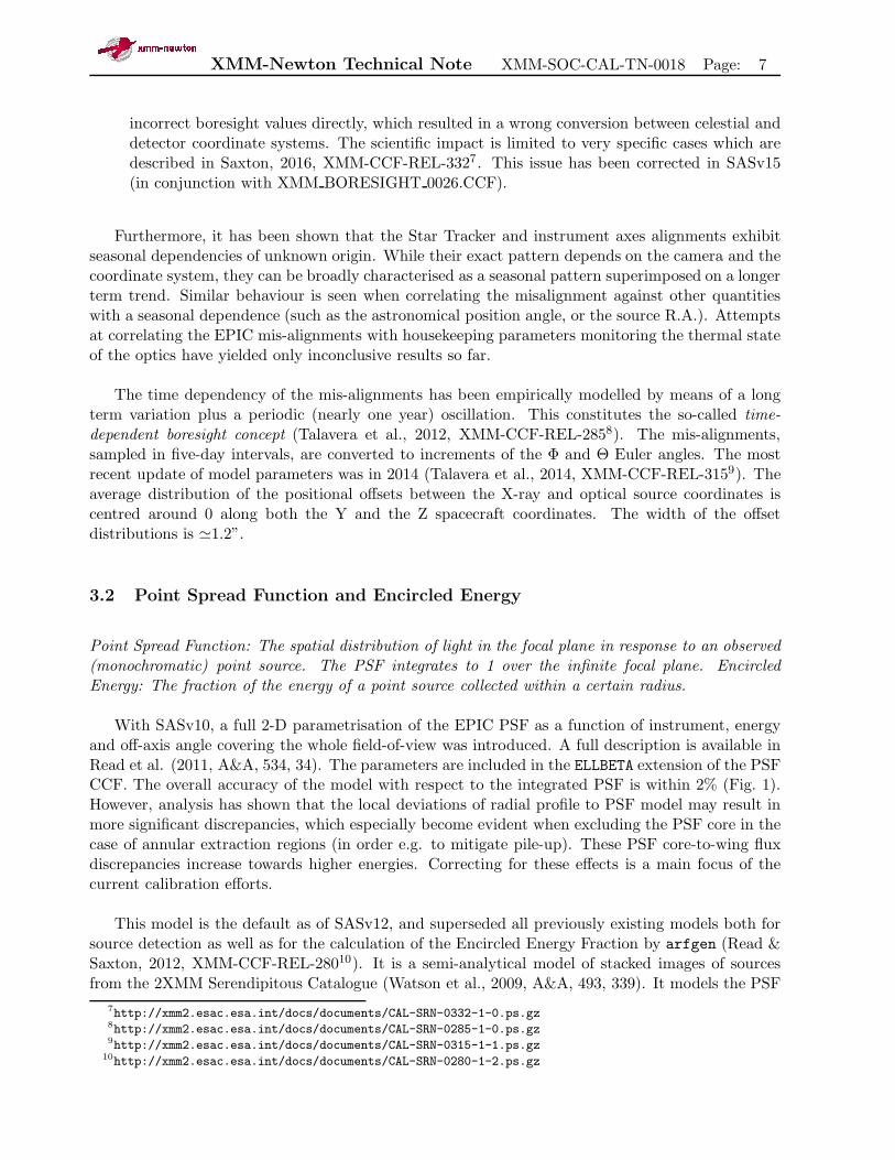
3.2 Point Spread Function and Encircled Energy

Point Spread Function: The spatial distribution of light in the focal plane in response to an observed(monochromatic) point source. The PSF integrates to 1 over the infinite focal plane. EncircledEnergy: The fraction of the energy of a point source collected within a certain radius.

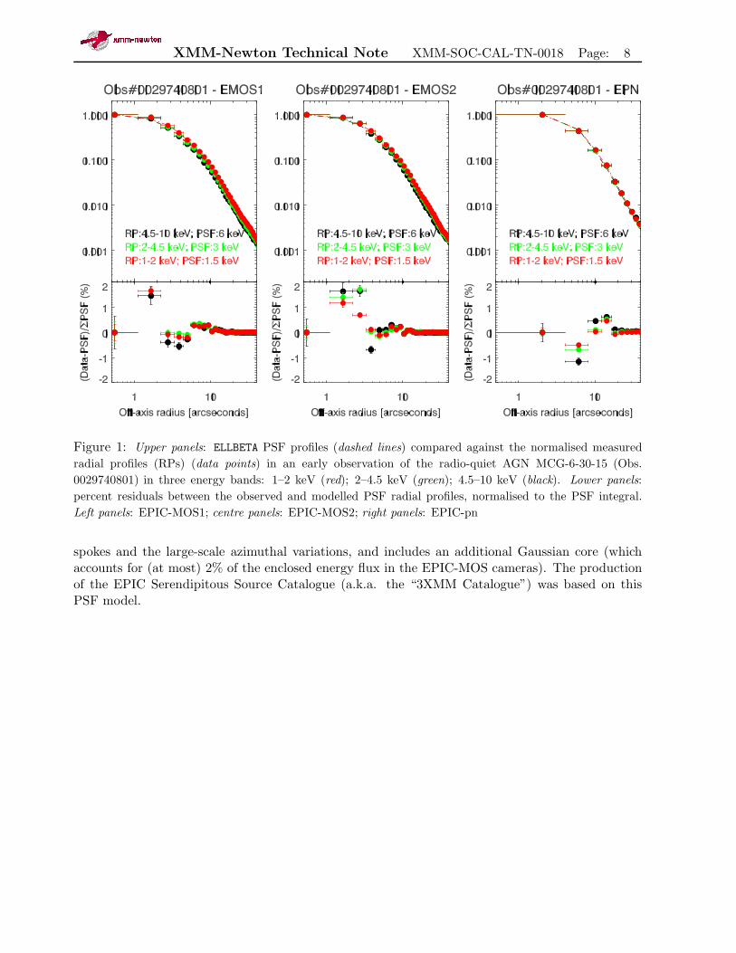
With SASv10, a full 2-D parametrisation of the EPIC PSF as a function of instrument, energyand off-axis angle covering the whole field-of-view was introduced. A full description is available inRead et al. (2011, A&A, 534, 34). The parameters are included in the ELLBETA extension of the PSFCCF. The overall accuracy of the model with respect to the integrated PSF is within 2% (Fig. 1).However, analysis has shown that the local deviations of radial profile to PSF model may result inmore significant discrepancies, which especially become evident when excluding the PSF core in thecase of annular extraction regions (in order e.g. to mitigate pile-up). These PSF core-to-wing fluxdiscrepancies increase towards higher energies. Correcting for these effects is a main focus of thecurrent calibration efforts.

This model is the default as of SASv12, and superseded all previously existing models both forsource detection as well as for the calculation of the Encircled Energy Fraction by arfgen (Read &Saxton, 2012, XMM-CCF-REL-28010). It is a semi-analytical model of stacked images of sourcesfrom the 2XMM Serendipitous Catalogue (Watson et al., 2009, A&A, 493, 339). It models the PSF

7http://xmm2.esac.esa.int/docs/documents/CAL-SRN-0332-1-0.ps.gz8http://xmm2.esac.esa.int/docs/documents/CAL-SRN-0285-1-0.ps.gz9http://xmm2.esac.esa.int/docs/documents/CAL-SRN-0315-1-1.ps.gz

10http://xmm2.esac.esa.int/docs/documents/CAL-SRN-0280-1-2.ps.gz


Figure 1: Upper panels: ELLBETA PSF profiles (dashed lines) compared against the normalised measured

radial profiles (RPs) (data points) in an early observation of the radio-quiet AGN MCG-6-30-15 (Obs.

0029740801) in three energy bands: 1–2 keV (red); 2–4.5 keV (green); 4.5–10 keV (black). Lower panels:

percent residuals between the observed and modelled PSF radial profiles, normalised to the PSF integral.

Left panels: EPIC-MOS1; centre panels: EPIC-MOS2; right panels: EPIC-pn

spokes and the large-scale azimuthal variations, and includes an additional Gaussian core (whichaccounts for (at most) 2% of the enclosed energy flux in the EPIC-MOS cameras). The productionof the EPIC Serendipitous Source Catalogue (a.k.a. the “3XMM Catalogue”) was based on thisPSF model.


4 Effective Area

Effective Area: the collecting area of the optical elements folded with the energy-dependent sensitivityof the detector systems of the EPIC cameras.

Figure 2: Distribution of residuals against

the best-fit logarithmic power-law model on

a sample of 90 observations of radio-loud

AGN extracted from the XMM-Newton

cross-calibration database (Stuhlinger et al.,

2010, XMM-SOC-CAL-TN-0052)

The internal accuracy in the determination of the totaleffective area over the spectral range from 0.4–12 keV isbetter than 3% and 2% (at 1-σ) for the EPIC-MOS andEPIC-pn cameras respectively (see Fig. 2).

The cross calibration between EPIC-MOS1 and EPIC-MOS2 agrees within 4%. The MOS/pn global flux normal-isation agrees to 8% from 0.4 keV to 12 keV. A statisti-cal assessment of the relative flux cross-calibration amongthe X-ray cameras on board XMM-Newton is discussed inStuhlinger et al. (2010, XMM-SOC-CAL-TN-005211) andRead et al. (2014, A&A, 564, 75).

As of SASv14.0, a non-default option allows an em-pirically derived correction to be applied to the EPICeffective areas (Guainazzi et al., 2014, XMM-CCF-REL-32112). This CORRAREA correction can be used to evaluatethe impact of the current relative uncertainties in the effec-tive area calibration on parameters derived from spectralfitting. Although this allows to estimate the effect of thesesystematic errors, it is emphasised that, pending furthervalidation, this correction is not meant to be used as a re-placement of the nominal calibration. The CORRAREA cor-rection can be invoked through the applyxcaladjusment

option in the arfgen task.

4.1 Mirror Collecting Area

Mirror collecting area: the face-on area of the mirror system that reflects X-rays to the focal region.

The mirror collecting area has been measured onground and verified in orbit. However, XMM-Newton EPIC-pn observations with very high statisticsstill showed residuals above 6 keV. For the latest calibration, readers are referred to Kirsch (2006,XMM-CCF-REL-20513).

11http://xmm2.esac.esa.int/docs/documents/CAL-TN-0052.ps.gz12http://xmm2.esac.esa.int/docs/documents/CAL-SRN-0321-1-2.ps.gz13http://xmm2.esac.esa.int/docs/documents/CAL-SRN-0205-1-0.ps.gz


4.2 Filter Transmission

Filter transmission: the fraction of incident X-ray photons that pass through the filter.

The filter transmission has been measured on ground. Fig. 3 shows filter transmission curves forall the cameras. For the thick filter the green curve shows the single transmission function currentlyused in the CCFs for MOS1, MOS2 and pn.

Figure 3: Filter transmission in CCF and in ground calibration filter measurement data points. Green:

THICK; red: MEDIUM; blue: THIN. Ground measurements are labelled with symbols: stars: EPIC-MOS1;

diamonds: EPIC-MOS2; squares: EPIC-pn. The CCF values are indicated by the dashed lines.

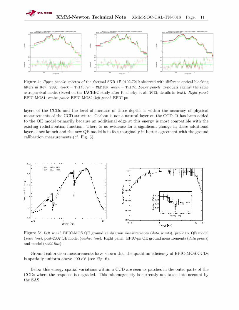
In Autumn 2012 a specific calibration experiment was performed on the thermal SNR 1E 0102-7219 to test in-flight the accuracy in the calibration of the filter transmission. The results aresummarised in Fig. 4. For all cameras and all filters, the residuals against the same astrophysicalmodel (Plucinsky et al. 2012, SPIE, 8443, 12) with the same parameters tied together are consistentwithin statistics (i.e. within ±1%).

4.3 CCD Quantum Efficiency

Quantum Efficiency (QE): the fraction of incident photons on the detector that generate an eventin the CCD.

Recalibration of the EPIC-MOS QE (Sembay, 2007, XMM-CCF-REL-23514) in 2007 led to anincrease of the surface layers of C, N and O. Nitrogen and Oxygen are constituents of the surface



0.1

1

10

Cts

/s/k

eV

Black: Thin, Red:Medium, Green:Thick1E0102−72.3 − XMM−Newton − EPIC−EMOS1 (XMMEA) − Model=IACHEC(v1.9)

10.50.8

0.9

1

1.1

1.2

Dat

a/m

odel

Energy (keV)

0.1

1

10

Cts

/s/k

eV

Black: Thin, Red:Medium, Green:Thick1E0102−72.3 − XMM−Newton − EPIC−EMOS2 (XMMEA) − Model=IACHEC(v1.9)

10.50.8

0.9

1

1.1

1.2

Dat

a/m

odel

Energy (keV)

1

10

Cts

/s/k

eV

Black: Thin, Red:Medium, Green:Thick1E0102−72.3 − XMM−Newton − EPIC−EPN (XMMEA) − Model=IACHEC(v1.9)

10.50.8

0.9

1

1.1

1.2

Dat

a/m

odel

Energy (keV)

Figure 4: Upper panels: spectra of the thermal SNR 1E 0102-7219 observed with different optical blocking

filters in Rev. 2380: black = THIN; red = MEDIUM; green = THICK. Lower panels: residuals against the same

astrophysical model (based on the IACHEC study after Plucinsky et al. 2012; details in text). Right panel:

EPIC-MOS1; centre panel: EPIC-MOS2; left panel: EPIC-pn.

layers of the CCDs and the level of increase of these depths is within the accuracy of physicalmeasurements of the CCD structure. Carbon is not a natural layer on the CCD. It has been addedto the QE model primarily because an additional edge at this energy is most compatible with theexisting redistribution function. There is no evidence for a significant change in these additionallayers since launch and the new QE model is in fact marginally in better agreement with the groundcalibration measurements (cf. Fig. 5).

Figure 5: Left panel, EPIC-MOS QE ground calibration measurements (data points), pre-2007 QE model

(solid line), post-2007 QE model (dashed line). Right panel: EPIC-pn QE ground measurements (data points)

and model (solid line).

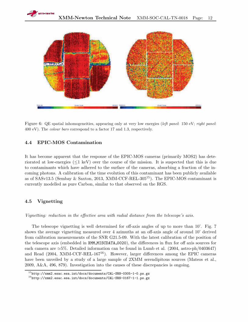
Ground calibration measurements have shown that the quantum efficiency of EPIC-MOS CCDsis spatially uniform above 400 eV (see Fig. 6).

Below this energy spatial variations within a CCD are seen as patches in the outer parts of theCCDs where the response is degraded. This inhomogeneity is currently not taken into account bythe SAS.


Figure 6: QE spatial inhomogeneities, appearing only at very low energies (left panel: 150 eV; right panel:

400 eV). The colour bars correspond to a factor 17 and 1.3, respectively.

4.4 EPIC-MOS Contamination

It has become apparent that the response of the EPIC-MOS cameras (primarily MOS2) has dete-riorated at low-energies (≤1 keV) over the course of the mission. It is suspected that this is dueto contaminants which have adhered to the surface of the cameras, absorbing a fraction of the in-coming photons. A calibration of the time evolution of this contaminant has been publicly availableas of SASv13.5 (Sembay & Saxton, 2013, XMM-CCF-REL-30515). The EPIC-MOS contaminant iscurrently modelled as pure Carbon, similar to that observed on the RGS.

4.5 Vignetting

Vignetting: reduction in the effective area with radial distance from the telescope’s axis.

The telescope vignetting is well determined for off-axis angles of up to more than 10’. Fig. 7shows the average vignetting measured over 4 azimuths at an off-axis angle of around 10’ derivedfrom calibration measurements of the SNR G21.5-09. With the latest calibration of the position ofthe telescope axis (embedded in XMM MISCDATA 0020), the differences in flux for off axis sources foreach camera are ≃5%. Detailed information can be found in Lumb et al. (2004, astro-ph/0403647)and Read (2004, XMM-CCF-REL-16716). However, larger differences among the EPIC camerashave been unveiled by a study of a large sample of 2XMM serendipitous sources (Mateos et al.,2009, A&A, 496, 879). Investigation into the causes of these discrepancies is ongoing.

15http://xmm2.esac.esa.int/docs/documents/CAL-SRN-0305-1-0.ps.gz16http://xmm2.esac.esa.int/docs/documents/CAL-SRN-0167-1-1.ps.gz


Figure 7: Average vignetting measured over 4 azimuths at an off-axis angle of around 10’ derived from the

calibration measurements of G21.5-0.9

5 Energy Redistribution

Energy Redistribution: The energy profile recorded by the detector system in response to a monochro-matic input. This includes the spreading of the recorded energy due to the statistical nature of chargecollection (i.e. the energy resolution) and also charge loss effects, which distort the profile.

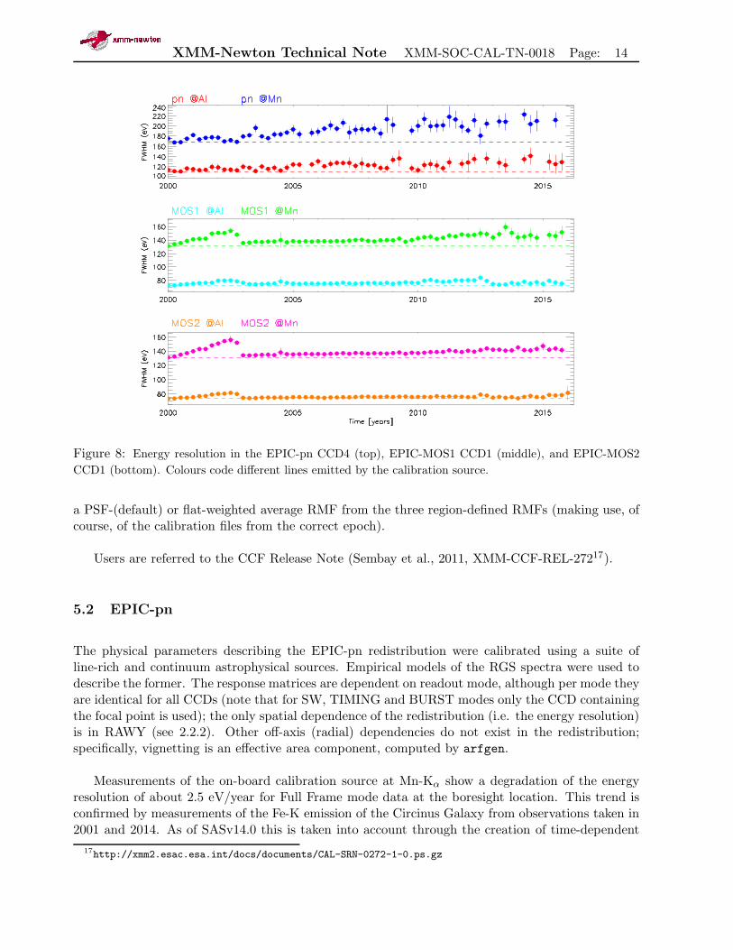
The energy resolution is monitored by the on-board calibration source, which produces strongAl-Kα (1.487 keV) and Mn-Kα (5.893 keV) emission lines. The resolution of the EPIC-MOS camerasdegraded significantly with time up to the epoch where the cameras were cooled (Fig. 8). After thisepoch the degradation in energy resolution has been small. For the EPIC-pn camera, the line widthat Mn-Kα increases by ≃2.5 eV/year. As of SASv14.0 this decrease in resolution is taken intoaccount through a time-dependent response function.

Pre-calculated (“canned”) redistribution matrices for most instrumental configurations, and arange of source positions and observation epochs are available at:http://www.cosmos.esa.int/web/xmm-newton/epic-response-files.

5.1 EPIC-MOS

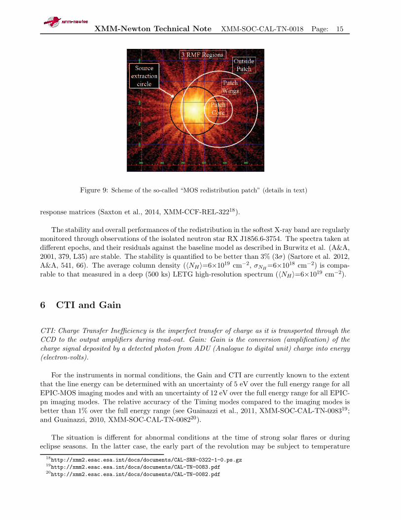
The low energy redistribution function (RMF) of the EPIC-MOS CCDs has a complex shape, inthat the main photo peak has a secondary component (a shoulder) which relatively increases withdecreasing energy, until, at the very lowest energies, it is the dominant component. Observations ofnon- or weakly-varying sources, such as the SNR 1E 0102-7219 and the O-star ζ Puppis, have shownthat the shape of the in-flight redistribution function changes both spatially across the detector (thechange from the on-ground calibration being most pronounced at the boresight) and also evolveswith observation epoch (Read et al. 2005, ESA-SP 604). The form of this was such that the originalshoulder evolved into a flatter ‘shelf’, of lower amplitude, but extending to lower energies. The bulkof the spatial change occurs within 40 arc-seconds of the boresight, a region which we refer to as the”patch”. A new method of deriving the RMF was incorporated in SASv11.0. There are three RMFregions on each of the two EPIC-MOS detectors; a ”patch core” region, a ”patch wings” regionand an ”outside patch” region (see Fig. 9). This, in combination with the 13 temporal epochs nowconsidered in the SAS, two types of PATTERN selection (single events and standard PATTERN<13) andtwo cameras gives rise to a total of 156 EPIC-MOS RMFs in the current calibration files. For asource extracted close to the patch (e.g., as in figure with patch), rmfgen automatically constructs


Figure 8: Energy resolution in the EPIC-pn CCD4 (top), EPIC-MOS1 CCD1 (middle), and EPIC-MOS2

CCD1 (bottom). Colours code different lines emitted by the calibration source.

a PSF-(default) or flat-weighted average RMF from the three region-defined RMFs (making use, ofcourse, of the calibration files from the correct epoch).

Users are referred to the CCF Release Note (Sembay et al., 2011, XMM-CCF-REL-27217).

5.2 EPIC-pn

The physical parameters describing the EPIC-pn redistribution were calibrated using a suite ofline-rich and continuum astrophysical sources. Empirical models of the RGS spectra were used todescribe the former. The response matrices are dependent on readout mode, although per mode theyare identical for all CCDs (note that for SW, TIMING and BURST modes only the CCD containingthe focal point is used); the only spatial dependence of the redistribution (i.e. the energy resolution)is in RAWY (see 2.2.2). Other off-axis (radial) dependencies do not exist in the redistribution;specifically, vignetting is an effective area component, computed by arfgen.

Measurements of the on-board calibration source at Mn-Kα show a degradation of the energyresolution of about 2.5 eV/year for Full Frame mode data at the boresight location. This trend isconfirmed by measurements of the Fe-K emission of the Circinus Galaxy from observations taken in2001 and 2014. As of SASv14.0 this is taken into account through the creation of time-dependent



Figure 1-11: The 3 different RMF regions

Figure 9: Scheme of the so-called “MOS redistribution patch” (details in text)

response matrices (Saxton et al., 2014, XMM-CCF-REL-32218).

The stability and overall performances of the redistribution in the softest X-ray band are regularlymonitored through observations of the isolated neutron star RX J1856.6-3754. The spectra taken atdifferent epochs, and their residuals against the baseline model as described in Burwitz et al. (A&A,2001, 379, L35) are stable. The stability is quantified to be better than 3% (3σ) (Sartore et al. 2012,A&A, 541, 66). The average column density (〈NH〉=6×1019 cm−2, σNH

=6×1018 cm−2) is compa-rable to that measured in a deep (500 ks) LETG high-resolution spectrum (〈NH〉=6×1019 cm−2).

6 CTI and Gain

CTI: Charge Transfer Inefficiency is the imperfect transfer of charge as it is transported through theCCD to the output amplifiers during read-out. Gain: Gain is the conversion (amplification) of thecharge signal deposited by a detected photon from ADU (Analogue to digital unit) charge into energy(electron-volts).

For the instruments in normal conditions, the Gain and CTI are currently known to the extentthat the line energy can be determined with an uncertainty of 5 eV over the full energy range for allEPIC-MOS imaging modes and with an uncertainty of 12 eV over the full energy range for all EPIC-pn imaging modes. The relative accuracy of the Timing modes compared to the imaging modes isbetter than 1% over the full energy range (see Guainazzi et al., 2011, XMM-SOC-CAL-TN-008319;and Guainazzi, 2010, XMM-SOC-CAL-TN-008220).

The situation is different for abnormal conditions at the time of strong solar flares or duringeclipse seasons. In the latter case, the early part of the revolution may be subject to temperature

18http://xmm2.esac.esa.int/docs/documents/CAL-SRN-0322-1-0.ps.gz19http://xmm2.esac.esa.int/docs/documents/CAL-TN-0083.pdf20http://xmm2.esac.esa.int/docs/documents/CAL-TN-0082.pdf


deviations of the on-board electronics which result in variations in the detector gain. For the EPIC-pn, this is addressed through a temperature dependent gain correction (Kirsch et al., 2007, XMM-CCF-REL-22321) which has been implemented as default as of SASv7.1.2. For the EPIC-MOS, nosuch correction has been yet been derived. However, the effect of the EMAE (EPIC-MOS AnalogueElectronics) temperature excursions during scientific observations are usually small (MOS1:<10 eVat Mn-K and <5 eV at Al-K).

The accuracy of the energy reconstruction in imaging modes is mainly limited by the accuracyof the time-dependency correction to the gain and CTI. Regular updates of this “long-term CTI”correction are performed, based on the analysis of the calibration source spectra.

For EPIC-pn, SASv14.0 introduced an energy dependency in the long-term CTI correction.Previously, the modelling was based on the trend at Mn-Kα (∼ 5.9 keV). However, as the rateof increase of CTI is energy dependent, this led to an increasing energy overcorrection at lowerenergies. The new calibration includes an additional modelling based on the trend as measured atAl-Kα (Smith et al., 2014, XMM-CCF-REL-32322).

The most recent updates of the EPIC-MOS long-term CTI and gain corrections are discussed inStuhlinger (2012a, XMM-CCF-REL-27823; 2012b, XMM-CCF-REL-27924).

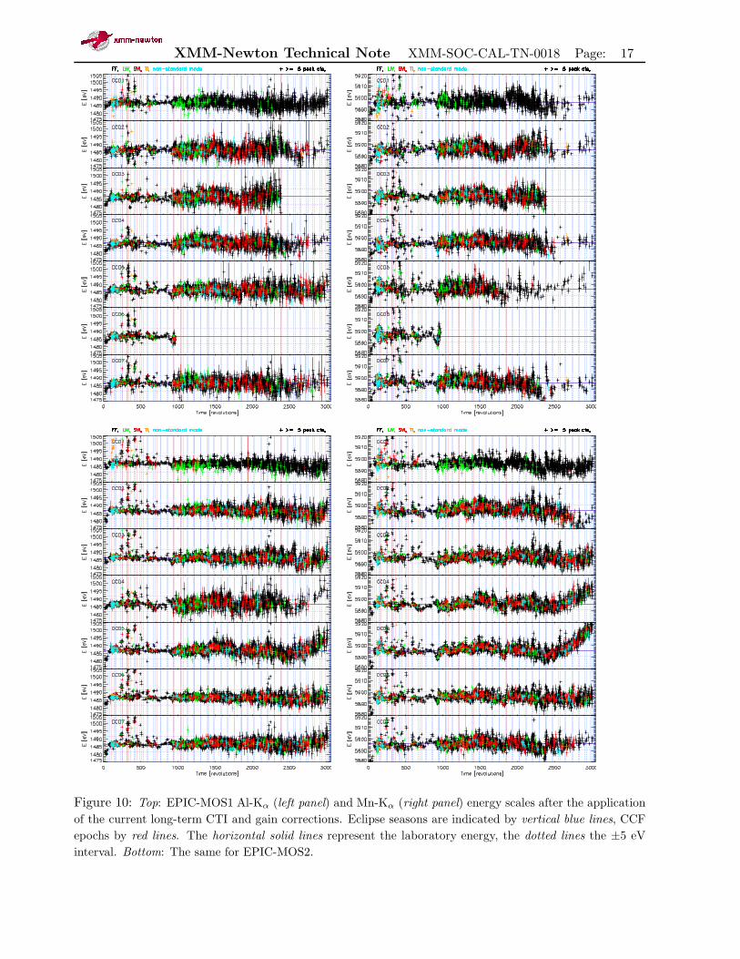
The calibration line energy reconstruction over the course of the mission is shown in Fig. 10 forEPIC-MOS and Fig. 11 for EPIC-pn.

7 Background

The XMM-Newton observatory provides good capabilities for detecting low surface brightness emis-sion features from extended and diffuse galactic and extragalactic sources, by virtue of the largefield of view of the X-ray telescopes and the high throughput yielded by the heavily nested telescopemirrors. In order to exploit the excellent EPIC data from extended objects, the EPIC background,now known to be higher than estimated pre-launch, has to be understood thoroughly.

Detailed information on the treatment of the EPIC background is provided on a dedicated webpage at the XMM-SOC portal at:http://www.cosmos.esa.int/web/xmm-newton/backgroundwhere several dedicated tools and filesare available for use in dealing with the EPIC background.

There are several different components to the EPIC background:

1. Photons

• The astrophysical background, dominated by thermal emission at lower energies (E<1 keV)

21http://xmm2.esac.esa.int/docs/documents/CAL-SRN-0223-1-0.ps.gz22http://xmm2.esac.esa.int/docs/documents/CAL-SRN-0323-1-1.ps.gz23http://xmm2.esac.esa.int/docs/documents/CAL-SRN-0278-1-1.ps.gz24http://xmm2.esac.esa.int/docs/documents/CAL-SRN-0279-1-0.ps.gz


Figure 10: Top: EPIC-MOS1 Al-Kα (left panel) and Mn-Kα (right panel) energy scales after the application

of the current long-term CTI and gain corrections. Eclipse seasons are indicated by vertical blue lines, CCF

epochs by red lines. The horizontal solid lines represent the laboratory energy, the dotted lines the ±5 eV

interval. Bottom: The same for EPIC-MOS2.


Figure 11: The same as Fig. 10 for EPIC-pn Mn-Kα (values are in ADU). Data from CCD 04 are taken

from the 20-row region around the boresight. The red vertical lines indicate the times of mayor solar coronal

mass ejections. The green horizontal lines indicate the nominal laboratory energy (drawn), and the ±3 ADU

interval (dashed).

and a power law at higher energies (primarily from unresolved cosmological sources). Thisbackground varies over the sky at lower energies.

• Solar wind charge exchange (Carter et al., 2011, A&A, 523, A115).

• Single reflections from outside the field of view, out-of-time events etc.

2. Particles

• Soft proton flares with spectral variations from flare to flare. This component can befiltered out by selecting quiet time periods from the data stream for analysis. To identifyintervals of flaring background the observer should generate a light curve of high energy(E>10 keV) single pixel (PATTERN=0) events. To identify good time intervals use theselection criteria:

– EPIC-MOS: <0.35 cts/s (#XMMEA EM && (PI>10000) && (PATTERN==0) on the fullFOV.

– EPIC-pn: <0.4 cts/s (#XMMEA EP && (PI>10000) && (PI<12000) && (PATTERN==0)

on the full FOV.

These selection criteria assume that sources above 10 keV do not contribute significantlyto the overall intensity


• Internal (cosmic-ray induced) background, created directly by particles penetrating theCCDs and indirectly by the fluorescence of satellite material to which the detectors areexposed.

3. Electronic Noise: Bright pixels and columns, readout noise, etc.

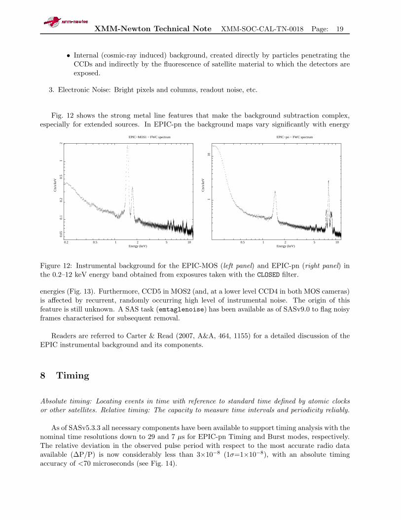
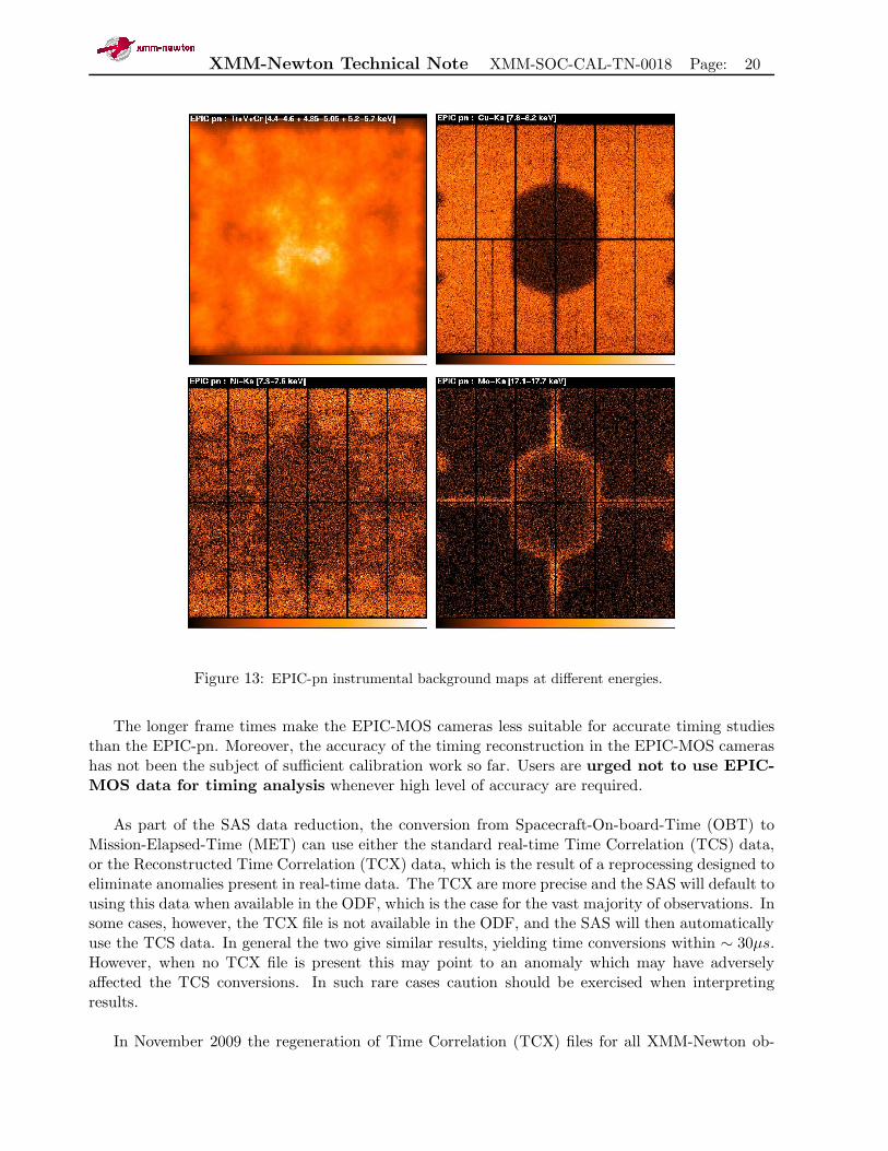
Fig. 12 shows the strong metal line features that make the background subtraction complex,especially for extended sources. In EPIC-pn the background maps vary significantly with energy

1 100.2 0.5 2 5

0.1

10.

050.

20.

52

Cts

/s/k

eV

Energy (keV)

EPIC−MOS1 − FWC spectrum

1 100.5 2 5

110

Cts

/s/k

eV

Energy (keV)

EPIC−pn − FWC spectrum

Figure 12: Instrumental background for the EPIC-MOS (left panel) and EPIC-pn (right panel) inthe 0.2–12 keV energy band obtained from exposures taken with the CLOSED filter.

energies (Fig. 13). Furthermore, CCD5 in MOS2 (and, at a lower level CCD4 in both MOS cameras)is affected by recurrent, randomly occurring high level of instrumental noise. The origin of thisfeature is still unknown. A SAS task (emtaglenoise) has been available as of SASv9.0 to flag noisyframes characterised for subsequent removal.

Readers are referred to Carter & Read (2007, A&A, 464, 1155) for a detailed discussion of theEPIC instrumental background and its components.

8 Timing

Absolute timing: Locating events in time with reference to standard time defined by atomic clocksor other satellites. Relative timing: The capacity to measure time intervals and periodicity reliably.

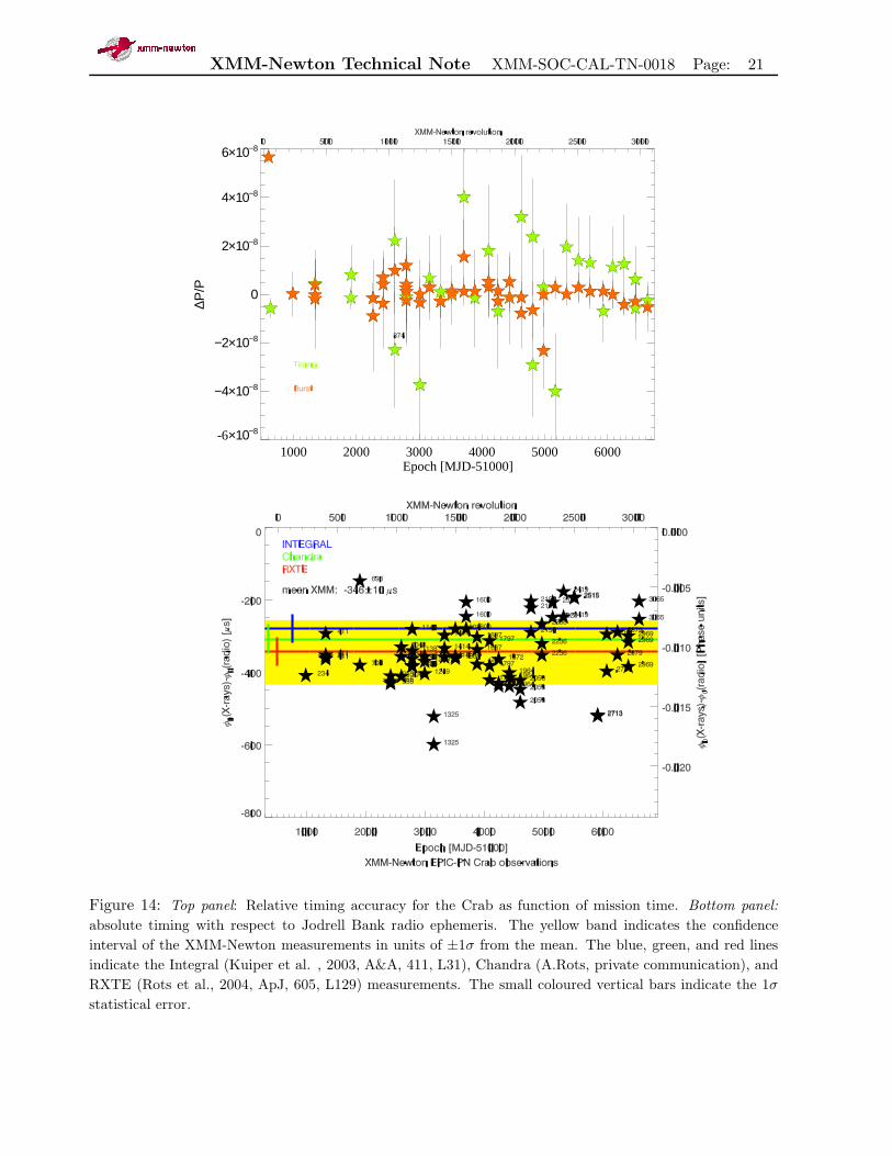
As of SASv5.3.3 all necessary components have been available to support timing analysis with thenominal time resolutions down to 29 and 7 µs for EPIC-pn Timing and Burst modes, respectively.The relative deviation in the observed pulse period with respect to the most accurate radio dataavailable (∆P/P) is now considerably less than 3×10−8 (1σ=1×10−8), with an absolute timingaccuracy of <70 microseconds (see Fig. 14).


Figure 13: EPIC-pn instrumental background maps at different energies.

The longer frame times make the EPIC-MOS cameras less suitable for accurate timing studiesthan the EPIC-pn. Moreover, the accuracy of the timing reconstruction in the EPIC-MOS camerashas not been the subject of sufficient calibration work so far. Users are urged not to use EPIC-

MOS data for timing analysis whenever high level of accuracy are required.

As part of the SAS data reduction, the conversion from Spacecraft-On-board-Time (OBT) toMission-Elapsed-Time (MET) can use either the standard real-time Time Correlation (TCS) data,or the Reconstructed Time Correlation (TCX) data, which is the result of a reprocessing designed toeliminate anomalies present in real-time data. The TCX are more precise and the SAS will default tousing this data when available in the ODF, which is the case for the vast majority of observations. Insome cases, however, the TCX file is not available in the ODF, and the SAS will then automaticallyuse the TCS data. In general the two give similar results, yielding time conversions within ∼ 30µs.However, when no TCX file is present this may point to an anomaly which may have adverselyaffected the TCS conversions. In such rare cases caution should be exercised when interpretingresults.

In November 2009 the regeneration of Time Correlation (TCX) files for all XMM-Newton ob-


1000 2000 3000 4000 5000 6000Epoch [MJD-51000]

-6×10−8

−4×10−8

−2×10−8

0

2×10−8

4×10−8

6×10−8

∆P/P

Figure 14: Top panel: Relative timing accuracy for the Crab as function of mission time. Bottom panel:

absolute timing with respect to Jodrell Bank radio ephemeris. The yellow band indicates the confidence

interval of the XMM-Newton measurements in units of ±1σ from the mean. The blue, green, and red lines

indicate the Integral (Kuiper et al. , 2003, A&A, 411, L31), Chandra (A.Rots, private communication), and

RXTE (Rots et al., 2004, ApJ, 605, L129) measurements. The small coloured vertical bars indicate the 1σ

statistical error.


servations after Rev. 300 was completed. Users are recommended to use the latest ODF (availableby default in the XSA) whenever they need the highest possible timing accuracy for the scientificgoals of their XMM-Newton data analysis.

An improved algorithm to detect and correct sporadic “jumps” in the flow of the photon ar-rival times as registered by the EPIC-pn camera has been implemented in SASv13.5. It is basedon a recalibration of the time evolution of the frame time due to a slow non-linear degradationof the on-board oscillator (Saxton & Freyberg, 2013, XMM-CCF-REL-29525). In the event of aEPIC-pn exposure being affected by a time jump (as indicated by the output of epframes withSAS VERBOSITY≥5), the user is encouraged to contact the Science Operation Centre helpdesk(http://www.cosmos.esa.int/web/xmm-newton/xmm-newton-helpdesk) for advice.

9 Cross Calibration

A dedicated Cross-Calibration Document (Stuhlinger et al., 2010, XMM-SOC-CAL-TN-005226) de-scribes the methods and data samples used in determining the cross-calibration status of the XMM-Newton instruments. The results presented in this document were obtained using SASv10 (December2010). More recent results may be found in e.g. presentations made at the Users’ Group meet-ings (http://www.cosmos.esa.int/web/xmm-newton/users-group). The cross-calibration statusof the XMM-Newton instruments as of SASv15 (February 2016) can be summarised as follows:

• At energies < 0.54 keV (fluorescent photo-absorption edge of neutral Oxygen) RGS yieldsfluxes typically 3% larger than those of EPIC-pn.

• At energies > 0.54 keV RGS yields fluxes typically 4% lower than EPIC-pn.

• At energies < 0.85 keV EPIC-MOS and EPIC-pn yield consistent fluxes.

• At energies > 0.85 keV EPIC-MOS yields typically 7% higher fluxes than EPIC-pn.

The EPIC-MOS cameras yield typically mutually consistent fluxes over their whole energy band-pass.

10 Unexpected Events

10.1 Micrometeoroid Impacts

To date, EPIC has suffered five events which have resulted in permanent damage to the detectors.These events, ascribed to micrometeoroid impacts along the boresight, are characterised by a suddenand short optical flash and physical damage to the detectors. In three cases the lasting effect was

25http://xmm2.esac.esa.int/docs/documents/CAL-SRN-0298-1-0.ps26http://xmm2.esac.esa.int/docs/documents/CAL-TN-0052.ps.gz


limited to the appearance of individual bright pixels (October 2000 in EPIC-pn, September 2001 inEPIC-MOS1 and August 2002 in EPIC-MOS2). However two events additionally resulted in moreextensive damage: the loss of EPIC-MOS1 CCD6 and the appearance of a hot column passing veryclose to the EPIC-MOS1 boresight (Rev. 961 in March 2005, seehttp://www.cosmos.esa.int/web/xmm-newton/mos1-ccd6) and the loss of EPIC-MOS1 CCD3(Rev. 2382 in December 2012, see http://www.cosmos.esa.int/web/xmm-newton/mos1-ccd3).

In addition, few cases of flash events without associated damage have been detected (e.g. inRevs. 2370 in EPIC-MOS1 and 2468 in EPIC-MOS2).

The events are interpreted as micrometeoroid dust scattered off the mirror surface under grazingincidence and reaching the focal plane detector. The typical particle size is estimated at <1 micron.The origin is most probably interplanetary (or interstellar) dust but not linked to meteor showers,the latter having larger sizes and higher masses (see Abbey et al., ESA proceedings SP-604, Kirschet al., 2005, Proc. SPIE 5898). An experimental verification of a micrometeoroid impact in a dustaccelerator, performed by the EPIC-pn team (MPE), demonstrated that particles of micron sizecould be deflected by grazing incident optics onto the focal plane of CCD (see N. Meidinger, 2002,Proc. SPIE 4851, 243-254).

The above mentioned hot column on EPIC-MOS1 CCD1 is located at RAWX=318 and is dueto leaking from a defect approximately at (RAWX,RAWY)=(318,572) (in the SAS calibrated eventslist coordinate system) which has raised the column offset by approximately 20 ADU in imagingmodes, and several tens of ADU higher in Timing mode. As a consequence, many low energy noiseevents are shifted above the nominal threshold. As the column passes very close to the aim point(at 3 and 9 pixels distance when EPIC-pn or RGS are prime, respectively) a significant fraction ofthe target source PSF is affected.

With this situation left uncorrected, events in the column are in fact flagged by the SAS taskembadpixfind and masked out (together with the events in its neighbouring columns at either side)in the calibrated events list. Nevertheless, for imaging modes, as of Rev. 1044 the increased columnnoise is suppressed through a change of the on-board offset table: real events in this column, whichundergo a raised baseline due the leaking hot pixels, are then restored to the correct energy throughthe modified offset. This allowed the column (and its neighbours) to be used for science again.However, recent measurements indicate that the column offset is evolving with time, meaning thatin certain exposures the correction scheme does not restore the event energies. In these cases theevents in the hot column and its neighbours will be flagged and masked through the default SASprocessing.

For EPIC-MOS1 in Timing mode, the post-impact offset value is far too large to allow a mean-ingful correction via a modification of the on-board offset table. Nor does standard SAS processingflag or remove the hot column. Therefore, users are advised to explicitly discard the affected col-umn and its adjacent ones from the accumulation of any scientific products; please refer to the SASwatchout web page(http://www.cosmos.esa.int/web/xmm-newton/sas-watchout-mos1-timing) for a specific recipeon how to obtain a consistent set of spectral files and responses for these cases.


11 Data Analysis

This section provides an overview of the major calibration/SAS improvements in epochs correspond-ing to SAS version releases. Also included is a guideline of how to work with the different modes ofthe cameras.

11.1 New Features in SAS

11.1.1 SASv16.0

• The new task evqpb provides a quiescent particle background events file to be associated withany given EPIC science exposure.

• The task ebkgreg, originally introduced for EPIC-pn, has been upgraded to work on EPIC-MOS data as well.

11.1.2 SASv15.0

• Correction of the conversion between celestial and detector coordinate systems (see Sect. 3.1).

• A new task ebkgreg determines the most suitable position of the background region for anysource in an EPIC-pn image.

• Given a position in celestial coordinates, the new task eupper calculates the count rate upperlimit for any EPIC sky image.

• eboxdetect, the task for sliding box source detection, is now compatible with detector coor-dinate input.

• The metatask for slew data analysis, eslewchain, can now produce PNG files for each subim-age.

11.1.3 SASv14.0

• The CORRAREA empirical effective area correction can be invoked in arfgen (not default).

• Time-dependent EPIC-pn spectral response.

• Energy dependent EPIC-pn long-term CTI correction.

• EPIC-pn double-event energy correction.

• The rate-dependent PHA (RDPHA) correction, introduced in SASv13, is now taken as defaultfor EPIC-pn Timing mode.

• For EPIC-pn Burst mode, the rate-dependent CTI (RDCTI) correction now takes into accountthe effects of X-ray loading.


11.1.4 SASv13.5

• Calibration of the contamination layer time evolution affecting the EPIC-MOS effective area.

• Improved calibration of the degradation of the EPIC-pn on-board oscillator frequency.

• Re-calibration of the energy scale in EPIC-pn Timing mode (XRL: epreject; RDPHA:epevents).

11.1.5 SASv13.0

• New operational mode in rmfgen to correct for moderately piled-up spectra.

11.1.6 SASv12.0

• New task epspatialcti to calculate a spatial-dependent gain correction in EPIC-pn.

• Improved algorithm in arfgen to calculate the Encircled Energy Fraction in fast modes.

• Correction to a bug in emldetect, which has caused in the past a 0.7” systematic positionangle dependent shift in the source coordinates.

• ELLBETA PSF model is the default.

11.1.7 SASv11.0

• Refinement of EPIC-pn long-term CTI algorithm.

• EPIC-MOS redistribution.

11.1.8 SASv10.0

• Support of the 2-D PSF (non-default).

• EPIC spectral rebinning tool (specgroup).

• Flagging of uncalibrated EPIC spectral channels (specgroup).

11.1.9 SASv9.0

• Generation of radial profiles and comparison with the PSF model.

• Tagging of noisy EPIC-MOS CCD frames.

• EPIC spectra fluxing.


11.1.10 SASv8.0

• Improved EPIC-pn time jump detection algorithm.

• EPIC-pn rate-dependent CTI correction (default off).

• 2-D elliptical PSF parametrisation.

11.1.11 SASv7.1

• Refinement of the EPIC-MOS QE improving the cross calibration between EPIC-pn and EPIC-MOS. The EPIC-MOS cameras will return now an energy independent flux difference withrespect to the EPIC-pn of ±5-7%. Before EPIC-MOS fluxes have been lower than EPIC-pnat low energies (0.2–0.8 keV) and higher at high energies (2–10 keV).

11.1.12 SASv7.0

• Column dependent CTI/Gain correction, improving line widths by up to ≃15% for some cases.

• Improved EPIC source detection and parametrisation tasks, especially related to the detectionof extended sources. Robustness and efficiency have been increased, to make possible the2XMM Catalogue derivation, which is in final preparation at the time of this release.

• Inclusion of PSF correction for EPIC timing and burst modes in response matrix generation.

• Support for arbitrary uniform binning of EPIC-MOS and EPIC-pn spectra.

• EPIC-pn FIFO reset correction corrects exposure time for saturation of the on chip amplifierstage (<5% more flux).

• EPIC-pn quadrant box temperature correction (see CAL-SRN-223).

11.1.13 SASv6.5

• rmfgen: The EPIC-MOS response calibration has been improved, including modelling of spa-tial and temporal response dependencies. This, together with calibration improvements in thenewly released EPIC-pn calibration files, has as a result a much better cross-calibration amongthe EPIC instruments.

• EPIC source detection tasks have been upgraded to be more robust and efficient, with correctdetection likelihoods.

• EPIC-MOS bad-pixel finding task has been upgraded.

• EPIC meta-tasks emproc and epproc include now all the functionalities and filtering possibil-ities present in the PERL scripts emchain and epchain.


11.2 Data Analysis

In the next section some general recommendations for data analysis are provided. This includes:

• Where should data be taken from the CCD.

• Which energy range should be used.

• Which pattern range should be used.

• Which response matrix should be used.

• A general caveat about “counting mode” in EPIC-pn.

For detailed guidelines on XMM data analysis please use the SAS Users’ Guide athttp://xmm-tools.cosmos.esa.int/external/xmm user support/documentation/sas usg/USG

and the SAS data analysis threads at http://www.cosmos.esa.int/web/xmm-newton/sas-threads.

11.2.1 EPIC-MOS

• Imaging modes

– Source region: where appropriate.27

– Background region:

∗ For point sources: Background can be extracted from the same observation, fromanother region of the same CCD, off-axis, away from source counts.

∗ For extended sources: This is more complicated. Please have a look at explanatorynotes available on the XMM web site athttp://www.cosmos.esa.int/web/xmm-newton/background.

The ebkgreg task, compatible with EPIC-MOS as of SASv16, can be useful in providinga suitable background region for a given source region and events image.

– Energy range: 0.3-10.0 keV, however, both limits depend on the aims of the analysis. Ingeneral the user should use patterns 0-12. (See XMM-Newton Users Handbook section3.3.11 available athttp://xmm-tools.cosmos.esa.int/external/xmm user support/documentation/uhb/).However, single events can be used to minimise the effects (e.g. spectral distortion) ofpile-up. Single events can also be used for observations in which the best-possible spectralresolution is crucial and the corresponding loss of counts is not important. In additionthe user should only use events flagged as “good” by using (#XMMEA EM) in the selectionexpression window of xmmselect. When analysing spectra the user should use effectivearea files produced by the SAS task arfgen in conjunction with redistribution matricesproduced with the SAS task rmfgen.

27In the case of a high count rate point source an annular region may be useful to remove the piled-up PSF core.However, note that in order to avoid introducing systematic inaccuracies in flux, the radius of the excised core shouldbe at least 2.5 times the instrumental pixel size (1.1” for EPIC-MOS and 4.1” for EPIC-pn). Seehttp://www.cosmos.esa.int/web/xmm-newton/sas-thread-epatplot for details.


• Timing mode

– Source region: where appropriate.

– Background region: background subtraction will not usually be an issue for sources ob-served in timing mode. However because the timing strip is only 100 pixels wide, back-ground regions should be taken from the outer CCDs, which are collecting data in imagingmode.

– Energy range: 0.3-10.0 keV. Single events only for the source. Pattern 0, 1, 3 for thebackground region in outer CCDs. As for imaging mode, canned redistribution matricesvalid for timing mode are available and should be used with ARF files produced by theSAS. Due to the large offset values following the micrometeoroid impact in Rev. 961,the column at RAWX=318 in EPIC-MOS1 Timing mode should no longer be used forscience analysis. Depending on the observation, the adjacent one or two columns maybe affected as well. Users are advised to remove these columns from the accumulation ofany scientific products (see Section 10.1 for details).

11.2.2 EPIC-pn

• Imaging modes

– Source region: where appropriate.27

– Background region:

∗ For point sources: From the same observation but away from the source. Ideally theregion should have the same distance to the readout node (RAWY) as the source re-gion. This ensures that similar low-energy noise is subtracted, because this increasestowards the readout-node. Do not use the columns passing through the source toavoid out-of-time events from the source, i.e. do not use an annulus around the sourceregion. Note that since SASv6.0 it is possible to suppress the low-energy noise withthe task epreject.

∗ For extended sources: This is more complicated. Please have a look at explanatorynotes available on the XMM web site athttp://www.cosmos.esa.int/web/xmm-newton/background.

The ebkgreg task, introduced for EPIC-pn in SASv15, can be useful in providing asuitable background region for a given source region and events image.

– Energy range: 0.3 keV–15 keV For imaging purposes pattern 0-12 can in principle be used.However, since doubles (1-4), triples (5-8) and quadruples (9-12) (see XMM-Newton UsersHandbook section 3.3.11 available athttp://xmm-tools.cosmos.esa.int/external/xmm user support/documentation/uhb/)are only created above twice, three and four times the low-energy threshold, respectively,cleanest images are produced by excluding the energy range just above the thresholds.To produce a 0.2–10 keV image one may select singles from the whole energy band anddoubles only from 0.4 keV. FLAG==0 omits parts of the detector area like border pixels,columns with higher offset, etc. This may not be desired (and is unnecessary) in thecase of broadband images. For spectral analysis, response matrices are available only forsingles, doubles and singles+doubles. Higher order pattern types are of low statistical


significance, have degraded spectral resolution and are therefore not useful. Best spectralresolution is reached by selecting singles for the spectrum. FLAG==0 should be used forhigh accuracy to exclude border pixels (and columns with higher offset) for which thepattern type and the total energy is known with significantly inferior precision. Towardshigher energies, the fraction of doubles approaches that of singles and hence includingdoubles is recommended for increased statistics. If a sufficient number of counts are avail-able, singles and doubles spectra can be created separately and fitted simultaneously inXSPEC (with all parameters including normalisations linked together). One exception isthe Timing mode (see below).

To choose the valid energy band for the spectral fit it is highly recommended using thetask epatplot. It uses as input a spatially selected (source region) event file and plotsthe fractions of the various patterns as function of energy. Spectral analysis should onlybe done in the energy band(s) where single- (and double-) fractions match the expectedcurves. In some observations the low-energy noise can be high, restricting the usefulband at low energies. Deviations at medium energies indicate pile-up (more doubles thanexpected) and in such cases the inner part of the PSF in the source region should beexcluded for spectral analysis. (More information on the topic of the pile-up is availablein the XMM-Newton Users Handbook athttp://xmm-tools.cosmos.esa.int/external/xmm user support/documentation/uhb/),Section 3.3.9).

The user should use ARF files produced by the latest version of the SAS task arfgen

in conjunction with canned redistribution matrices (which are compatible to the CTIcorrection used in SASv5.3.3 or above) or produce those redistribution matrices with theSAS task rmfgen. For each readout mode of the EPIC-pn a set of RMF files is available(for singles, doubles, singles+doubles. Except timing mode where only singles+doublesmust be used). The CTI causes a dependence of spectral resolution with distance to thereadout node. Therefore the 200 lines of each CCD are divided into areas of 20 lines each(Y0 at readout, Y9 at opposite side, which includes the nominal focus point) and for eacharea an RMF file is available

• Timing and Burst modes

– Source region: Column range centred on the source position. In the Timing and Burstmodes the RAWY coordinate is related to the event time - any selection on RAWYwould therefore exclude certain time periods. For Timing mode no such selection shouldbe made and hence complete columns should be used. For Burst mode, however, a RAWYselection of RAWY<160 should be used to avoid direct illumination by the source.

– Background region: Column range covering a source-free region. For Timing mode,complete columns should be selected. For Burst mode, the identical RAWY selection asused in the source definition should be applied.

– Energy range: 0.7–10.0 keV (Timing mode), 0.6–10.0 keV (Burst mode)

– Pattern: For Timing mode only singles+doubles (patterns 0–4) should be used. For Burstmode combinations of singles and doubles may be used as in imaging modes.

Note that detailed instructions and caveats regarding the analysis of Burst mode data can befound in Kirsch et al., 2006, A&A, 453, 173.


11.2.3 Counting Mode

If the total (source plus background) count rate is above a certain limit (a few hundred counts/s),either because of the source being too bright or due to very high flaring background, the EPIC cam-eras will switch to the so-called ‘counting mode’, a special instrument mode where no transmissionof information for individual X-ray events occurs. SAS is able to correct for the dead-time yieldedby the counting mode intervals. Still it is advisable to minimise as much as possible the onset ofcounting mode, because its loss of scientifically usable exposure time. Using a windowing mode or(for soft sources) a thicker optical blocking filter may help.

Counting mode occurs at count rates larger than 30 (700) counts per second in imaging modes(Timing mode). It affects simultaneously all CCDs in the quadrant where it occurs. In exposurestaken in imaging modes it is more likely to occur at the beginning and at the end of XMM-Newtonrevolutions due to the higher background environment (see Fig. 15).

12 History of This Document

• Version 3.8 (12/12/2016)

– Aligned with SASv15.0 and SASv16.0

– Added paragraph on timing accuracy in the case no TCX is available

– Updated XMM cross-calibration summary

– Updated micrometeoroid impact section

– Added footnote cautioning against annular inner radii smaller than instrumental pixelsize

– Clarified TI and BU mode data analysis section, in particular that BU mode source andbackground regions must have identical RAWY selections

– Fig. 8 (EPIC energy resolution trends)

– Fig. 10 (MOS calibration line energy reconstruction)

– Fig. 11 (pn calibration line energy reconstruction)

– Fig. 14 (relative and absolute timing accuracy)

– Updated URLs in view of migration to Cosmos

• Version 3.7 (28/08/2015)

– Aligned with SASv14.0

– effective area: CORRAREA

– pn energy redistribution

– pn CTI/gain

– pn and MOS energy scale

– Figs. 10 and 11 (MOS calibration line energy reconstruction)

– Fig. 11 (pn calibration line energy reconstruction)


Figure 15: Fraction of exposure time affected by counting mode in EPIC-pn exposures as a function of count

rate (top panel) and orbital phase (bottom panel) for all exposures from Rev. 1180 to around Rev. 1900.

Instrumental modes are colour coded. The labels indicate the fraction of exposures affected by counting mode

(in brackets the same number if one considers only exposures where counting mode affects a fraction of the

total exposure time >5%).

– Fig. 14 (relative and absolute timing accuracy)

• Version 3.4 (26/08/2014)

– EPIC-MOS contamination calibration

– EPIC-pn Timing mode energy scale calibration

– Refined calibration of the EPIC-pn on-board oscillator frequency time evolution


– Fig. 1 (ELLBETA calibration accuracy)

– Fig. 2 (relative area calibration accuracy)

– Fig. 11 (EPIC-pn Mn Kα calibration line centroid history)

– Fig. 14 (timing accuracy)

• Version 3.3 (2/10/2013)

– Sect. 6 aligned to XMM-CCF-REL-300

• Version 3.2 (25/8/2013)

– Caveat on the EPIC-pn energy reconstruction in recent exposures

– Report on the experiment to test the accuracy of the filter transmission calibration (seeSect. 4.2)

– Stacked residuals on 2XMM sources as a (possible) metrics of the systematic uncertaintieson the effective area (see Sect. 4)

– Update of Fig. 14 with the latest results

– Caveat on the accuracy of timing reconstruction in EPIC-MOS (see Sect. 8)

– MOS1-CCD3 event (see Sect. 10)

• Version 3.1 (24/7/2012)

– Update of the Section on astrometry (including the “time-dependent boresight” imple-mentation)

– ELLBETA PSF model (see Sect. 3.2)

– New Fig. 10, 11, and 12 (long-term calibration source centroid energy monitoring results)

– Update of Fig. 8, and 14

• Version 3.0 (16/11/2011)

– text streamlining and conversion into a standard LATEX XMM-Newton document

• Version 2.13 (10/6/2011)

– Alignment to SASv11

– Updates of Fig. 12, 14

– New pn redistribution

– New MOS redistribution

– Update of the standard calibrated energy ranges for spectral fitting.

• Version 2.12 (10/1/2011):

– New Fig.1-7 (transmission filters cross-calibration)

– Updates of Fig. 12 using the most recent measurements

• Version 2.11 (18/07/2010)

– Fig.1.20 (counting mode in EPIC-pn)


• Version 2.10 (24/06/2010) - Aligned with SASv10.0

– 2-D PSF support in SASv10.0

– EPIC-pn redistribution refinement

– RAWY-dependent calibration of the PATTERN fraction in EPIC-pn Timing mode

– Schedule for the implementation of a refined EPIC-pn time jumps algorithm in the SAS

– specgroup

– Update of Fig. 12 (Timing accuracy) after the regeneration of TCX files

– Update of Fig.1-18 (cross-calibration status) to SASv9.0 results

• Version 2.9 (14/01/2010)

– Report on the discovery of a possible underestimation of the pn resolution at ≃6 keV

– Update Fig.1-17 (Timing accuracy) with the results of the October 2009 Routine Cali-bration Plan measurements

• Version 2.8 (30/07/2009) - Aligned with SASv9.0

– Update of ongoing calibration topics following the outcomes of 2009 EPIC CalibrationMeeting (presentation given at this meeting are available at:http://www.src.le.ac.uk/projects/xmm/technical/)

– Removal of Subsection: “Addendum: Off-axis PSF MOS speciality” of Sect. 1.1.2, nowsubsumed by Mateos et al. (2009, A&A, 496, 879)

– Inclusion of figure on the stability of pn soft X-rays redistribution (now superseded)

– Alignment of the left panel of Fig. 14 tohttp://xmm2.esac.esa.int/docs/documents/CAL-TN-0082.pdf

– Update of Fig.1-17 (Timing accuracy) with the results of the February 2009 RoutineCalibration Plan measurements

– SASv9.0 EPIC-related updates in Sect.2.1

epic status of calibration and data analysis

Documents