environmental impacts on the performance of pavement

A pooled fund project administered by the Minnesota Department of Transportation

Authors: Bora Cetin, Kristen Cetin, Tuncer Edil, Debrudra Mitra

Environmental Impacts on the Performance of Pavement Foundation Layers

Report No. NRRA202108

To request this document in an alternative format, such as braille or large print, call 651-366-4718 or 1-800-657-3774 (Greater Minnesota) or email your request to [email protected]. Please request at least one week in advance.

tel:651-366-4718

tel:1-800-657-3774

tel:1-800-657-3774

mailto:[email protected]

Technical Report Documentation Page

1. Report No. 2. 3. Recipients Accession No. NRRA202108

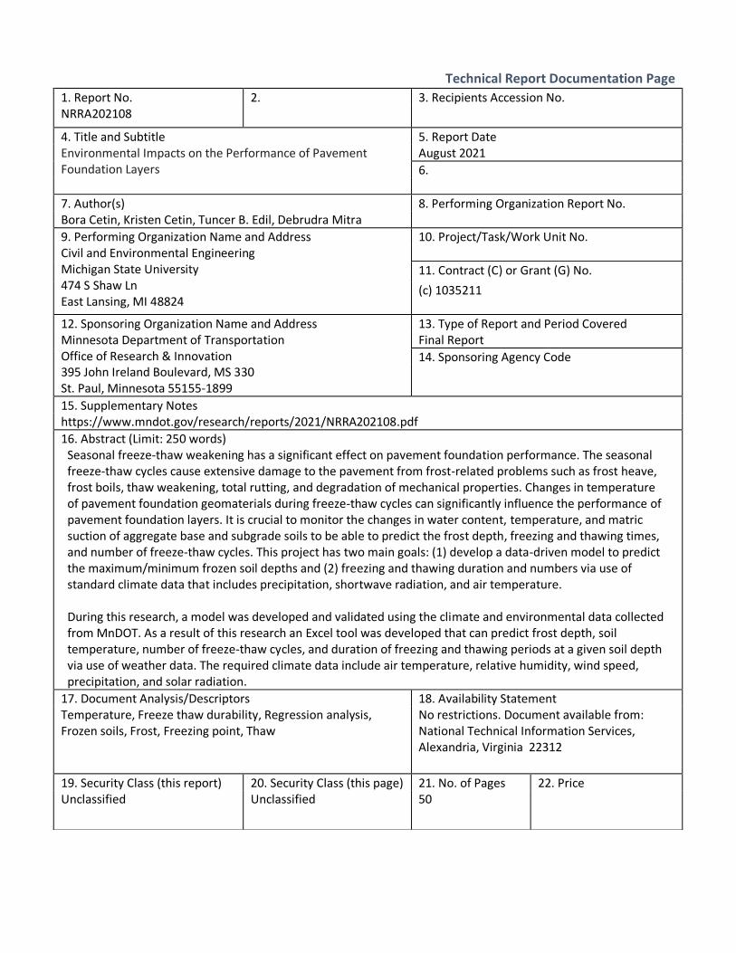
4. Title and Subtitle 5. Report Date Environmental Impacts on the Performance of Pavement August 2021 Foundation Layers 6.

7. Author(s) 8. Performing Organization Report No. Bora Cetin, Kristen Cetin, Tuncer B. Edil, Debrudra Mitra

9. Performing Organization Name and Address 10. Project/Task/Work Unit No. Civil and Environmental Engineering Michigan State University 474 S Shaw Ln East Lansing, MI 48824

11. Contract

(c) 1035211

(C) or Grant (G) No.

12. Sponsoring Organization Name and Address 13. Type of Report and Period Covered Minnesota Department of Transportation Office of Research & Innovation 395 John Ireland Boulevard, MS 330

Final Report

14.

Sponsoring Agency Code

St. Paul, Minnesota 55155-1899

15. Supplementary Notes https://www.mndot.gov/research/reports/2021/NRRA202108.pdf

16. Abstract (Limit: 250 words) Seasonal freeze-thaw weakening has a significant effect on pavement foundation performance. The seasonal freeze-thaw cycles cause extensive damage to the pavement from frost-related problems such as frost heave, frost boils, thaw weakening, total rutting, and degradation of mechanical properties. Changes in temperature of pavement foundation geomaterials during freeze-thaw cycles can significantly influence the performance of pavement foundation layers. It is crucial to monitor the changes in water content, temperature, and matric suction of aggregate base and subgrade soils to be able to predict the frost depth, freezing and thawing times, and number of freeze-thaw cycles. This project has two main goals: (1) develop a data-driven model to predict the maximum/minimum frozen soil depths and (2) freezing and thawing duration and numbers via use of standard climate data that includes precipitation, shortwave radiation, and air temperature. During this research, a model was developed and validated using the climate and environmental data collected from MnDOT. As a result of this research an Excel tool was developed that can predict frost depth, soil temperature, number of freeze-thaw cycles, and duration of freezing and thawing periods at a given soil depth via use of weather data. The required climate data include air temperature, relative humidity, wind speed, precipitation, and solar radiation.

17. Document Analysis/Descriptors 18. Availability Statement Temperature, Freeze thaw durability, Regression analysis, No restrictions. Document available from: Frozen soils, Frost, Freezing point, Thaw National Technical Information Services,

Alexandria, Virginia 22312

19. Security Class (this report) 20. Security Class (this page) 21. No. of Pages 22. Price Unclassified Unclassified 50

ENVIRONMENTAL IMPACTS ON THE PERFORMANCE OF PAVEMENT

FOUNDATION LAYERS

FINAL REPORT

Prepared by:

Bora Cetin, Associate Professor, Michigan State University

Kristen Cetin, Assistant Professor, Michigan State University

Tuncer B. Edil, Professor Emeritus, University of Wisconsin-Madison

Debrudra Mitra, Research Associate, Michigan State University

August 2021

Published by:

Minnesota Department of Transportation Office of Research & Innovation 395 John Ireland Boulevard, MS 330 St. Paul, Minnesota 55155-1899

This report represents the results of research conducted by the authors and does not necessarily represent the views or policies

of the Minnesota Department of Transportation or Michigan State University. This report does not contain a standard or

specified technique.

The authors, the Minnesota Department of Transportation, and Michigan State University do not endorse products or

manufacturers. Trade or manufacturers’ names appear herein solely because they are considered essential to this report.

ACKNOWLEDGMENTS

The authors would like to thank the National Road Research Alliance (NRRA) for sponsoring this project. The authors would also like to thank Liaison Tim Andersen, Minnesota DOT (MnDOT), and acknowledge members of the project Technical Advisory Panel (TAP): Terry Beaudry, MnDOT; Matt Oman, Mathy Construction; Heather Shoup, Illinois DOT (IDOT); and Raul Velasquez, MnDOT.

TABLE OF CONTENTS

CHAPTER 1. INTRODUCTION ................................................................................................................ 1

CHAPTER 2. DATASETS ......................................................................................................................... 2

CHAPTER 3. CALCULATION OF FREEZE-THAW CYCLES .......................................................................... 7

3.1. Fixed freezing temperature ...................................................................................................... 7

3.2. Modified reference temperature method ................................................................................ 9

3.3. Time delay method ................................................................................................................ 10

3.4. Recommendations ................................................................................................................. 12

CHAPTER 4. MODEL DEVELOPMENT .................................................................................................. 13

4.1. Data Processing ...................................................................................................................... 13

4.2. Model Development .............................................................................................................. 15

4.2.1. Temperature prediction ................................................................................................. 16

4.2.2. Prediction of number of freeze-thaw cycles .................................................................... 19

4.2.3. Isotherm calculation ....................................................................................................... 21

4.2.4. Time duration of freezing and thawing phase and their occurrence ................................ 22

CHAPTER 5. TOOL DEVELOPMENT ..................................................................................................... 29

5.1. Temperature Prediction ......................................................................................................... 31

5.2. Number of Freeze-Thaw Cycles .............................................................................................. 31

5.3. Predict Soil Temperature and Number of Freeze-Thaw Cycles ................................................ 31

5.4. Steps to Run the Tool ............................................................................................................. 32

CHAPTER 6. CONCLUSIONS AND RECOMMENDATIONS ...................................................................... 34

CHAPTER 7. REFERENCES ................................................................................................................... 35

APPENDIX A: FREEZE AND THAW INDEX FRONT AND EQUATION USED FOR TOOL DEVELOPMENT

LIST OF FIGURES

Figure 2.2 Moisture variation at different depths for locations (a) Cell 185, (b) Cell 186, (c) Cell 188, (d)

Cell 189, (e) Cell 127, (f) Cell 728 ............................................................................................................. 4

Figure 3.1 Freeze-thaw cycle diagram ...................................................................................................... 7

Figure 3.2: Variation in number of freeze-thaw cycles for different freezing point temperatures across 2

years of measured data for Cell 185 ........................................................................................................ 7

Figure 3.3: Average freeze-thaw cycles by month from a prior MnDOT study (MnDOT, 2014).................. 8

Figure 3.4: Average freeze-thaw cycles by month for (a) 3-inch and (b) 4-inch depth ............................... 9

Figure 3.5: Number of freeze-thaw cycles obtained using modified reference temperature method for

Cell 185 ................................................................................................................................................. 10

Figure 3.6: Schematic of the time delay scenario to calculate the number of freeze-thaw cycles ........... 11

Figure 3.7: Number of freeze-thaw cycles using the time delay method and an assumed -1°C freezing

point temperature ................................................................................................................................. 12

Figure 4.1. Temperature prediction using Vector Auto Regression Model .............................................. 16

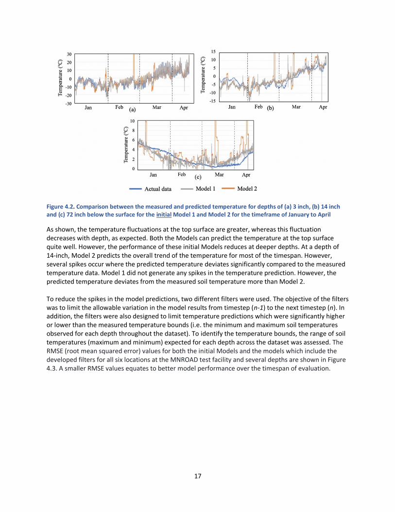
Figure 4.2. Comparison between the measured and predicted temperature for depths of (a) 3 inch, (b)

14 inch and (c) 72 inch below the surface for the initial Model 1 and Model 2 for the timeframe of

January to April ..................................................................................................................................... 17

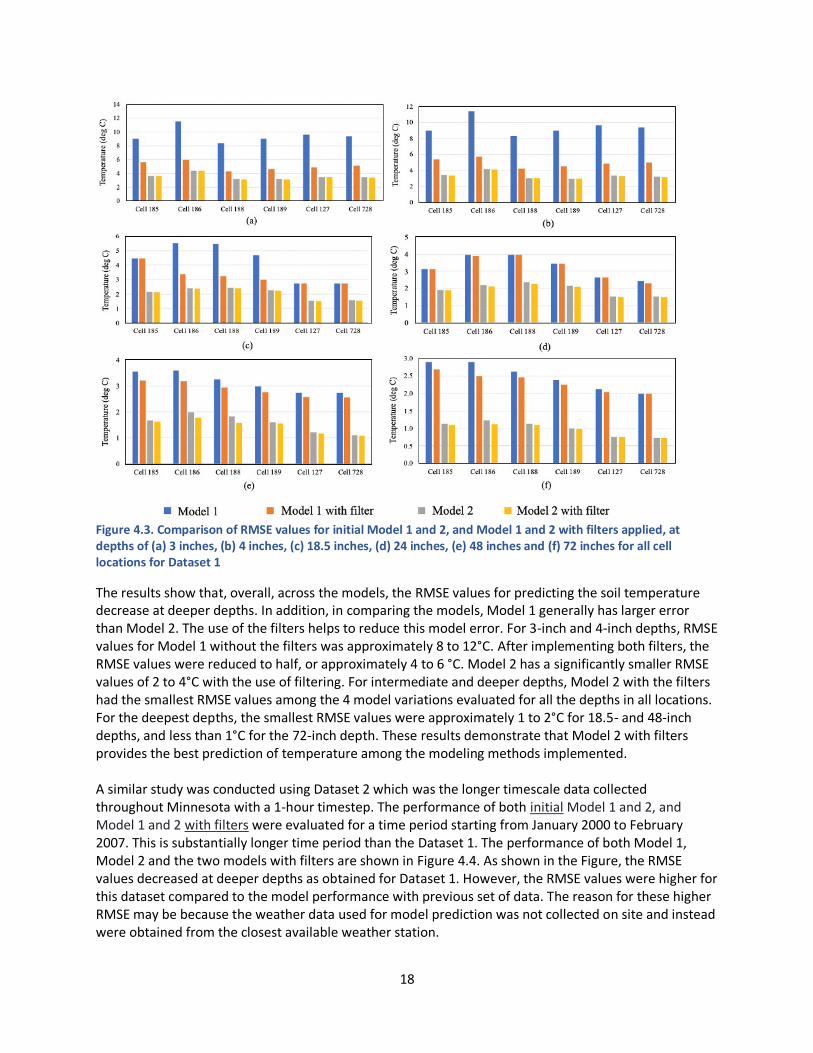
Figure 4.3. Comparison of RMSE values for initial Model 1 and 2, and Model 1 and 2 with filters applied,

at depths of (a) 3 inches, (b) 4 inches, (c) 18.5 inches, (d) 24 inches, (e) 48 inches and (f) 72 inches for all

cell locations for Dataset 1 .................................................................................................................... 18

Figure 4.4: Comparison of RMSE values for Dataset 2 ............................................................................ 19

Figure 4.5. Comparison of the freeze-thaw cycle variations for the four Models .................................... 20

Figure 4.6. Number of freeze-thaw cycle comparison for Dataset 2 ....................................................... 21

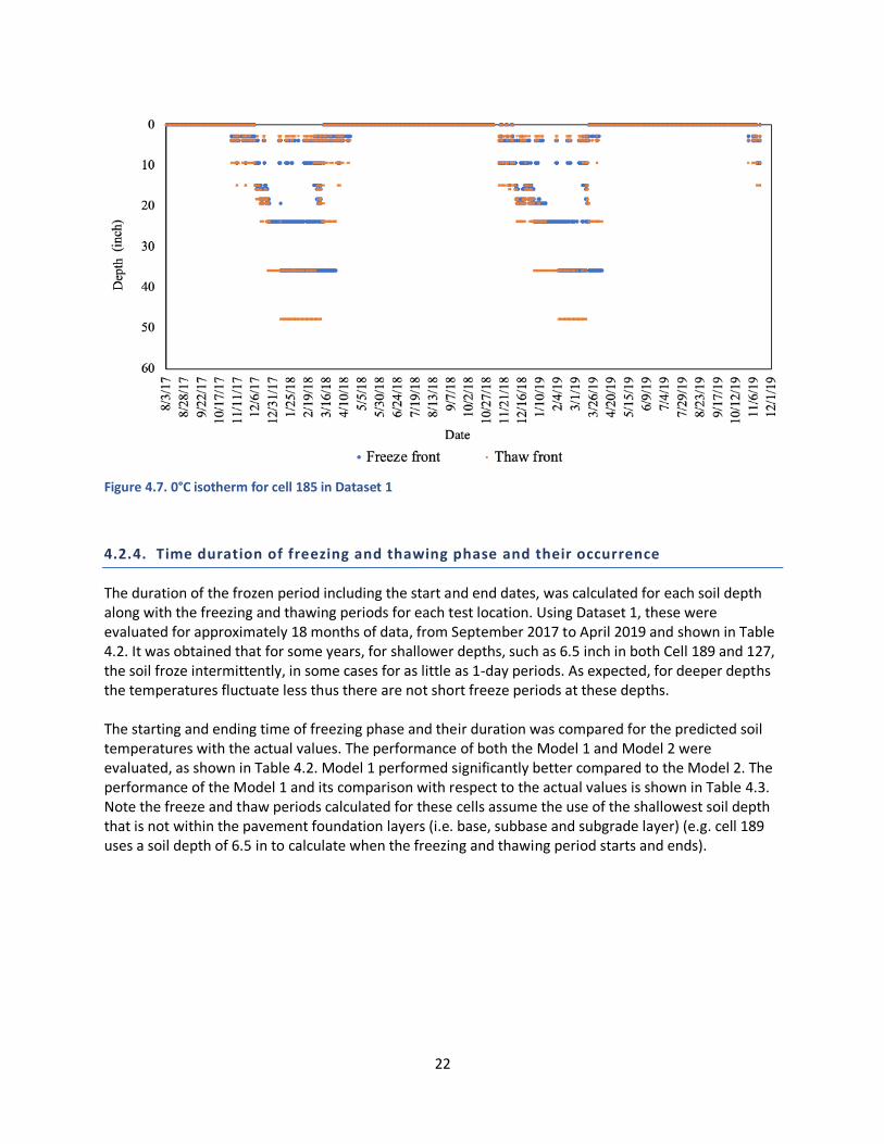
Figure 4.7. 0°C isotherm for cell 185 in Dataset 1 ................................................................................... 22

Figure 5.1: Framework of the Excel-based tool ...................................................................................... 29

Figure 5.2: Required input from the user ............................................................................................... 30

Figure 5.3: Soil depth input to the tool as a drop-down menu (in green, bottom right) .......................... 30

Figure 5.4. Example results of the ‘Temperature prediction’ button ....................................................... 31

Figure 5.5. Example results of the ‘Number of freeze-thaw cycles prediction’ button ............................. 31

Figure 5.6. Example results of the ‘Predict soil temperature and number of cycles’ button ..................... 32

Figure 5.7. Error message generated for out-of-range or non-numerical data input ............................... 32

Figure 5.8. Tool asking permission to run ............................................................................................... 32

Figure A.1. 0°C isotherm for test sites (a) cell 186, (b) cell 188, (c) cell 189, (d) cell 127 and (e) cell 728 in

LIST OF TABLES

Table 2.1 Soil depths for measured temperatures.................................................................................... 2

Table 2.2 Soil depths for moisture measurements ................................................................................... 2

Table 2.3: Data availability for different locations .................................................................................... 5

Table 2.4: Percentage of missing elements in the collected dataset in the MnROAD Test Cells ................ 5

Table 2.5: Percentage of missing elements in the MNDOT collected dataset ............................................ 6

Table 3.1. Reference temperature variation as defined by MnDOT Technical Memorandum 14-10-MAT-

02 and modified reference temperature by time of year ....................................................................... 10

Table 4.1 Correlation analysis using stepwise regression ....................................................................... 14

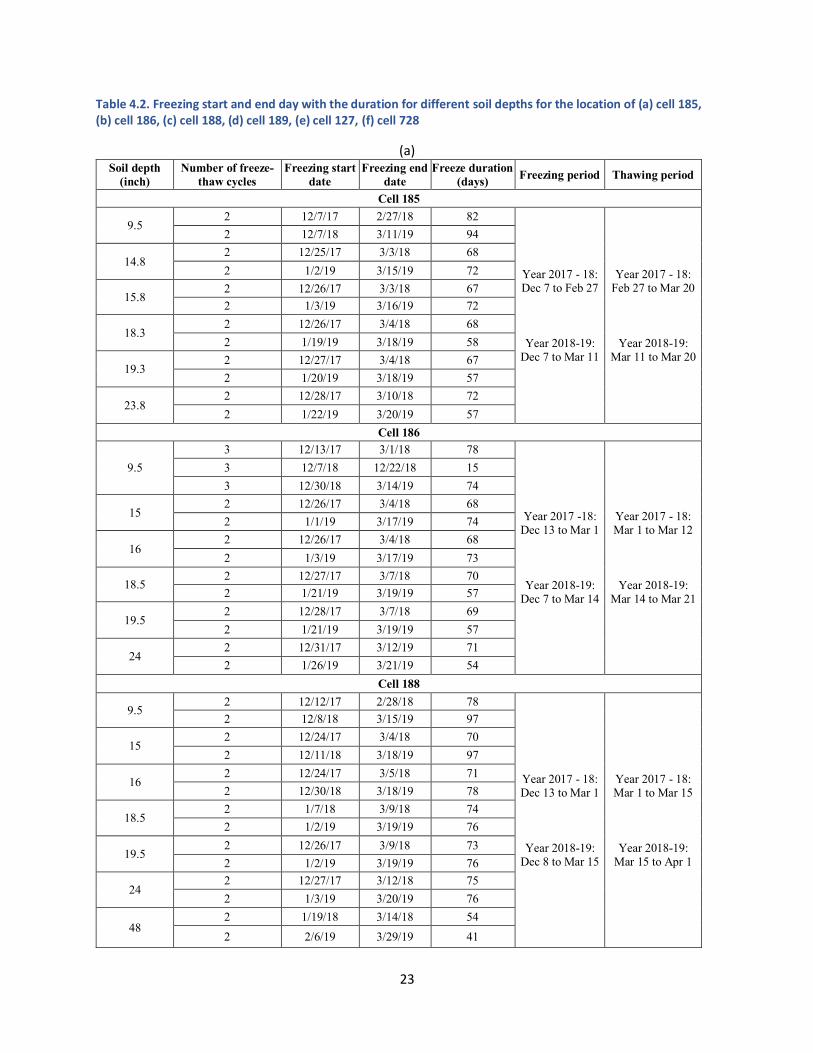
Table 4.2. Freezing start and end day with the duration for different soil depths for the location of (a)

cell 185, (b) cell 186, (c) cell 188, (d) cell 189, (e) cell 127, (f) cell 728 .................................................... 23

Table 4.3. Comparison of freezing time for actual and predicted soil temperatures for Dataset 1 for the

location of (a) cell 185, (b) cell 186, (c) cell 188, (d) cell 189, (e) cell 127, (f) cell 728 (note: Method 1

refers to Model1) .................................................................................................................................. 25

Table 4.4. Comparison of freezing and thawing period for all cell locations using Dataset 1 ................... 28

EXECUTIVE SUMMARY

Seasonal freeze-thaw action and changes in temperature from environmental fluctuations have a significant effect on soil behavior. Seasonal freeze-thaw cycles and water migration create radical changes in soil-structure systems through frost heave, frost boils, thaw weakening, and settlement. It is crucial to monitor the changes in soil temperature to predict the frost depth, freezing and thawing duration, strength, and moduli. Such physics-based models require an extensive amount of data that can be tedious to collect. These models require site-specific soil profiles and ground sensor data that are not commonly available and can be costly to obtain. Moreover, these models are constrained by the limitations and assumptions inherent with the method of solution as well as boundary conditions. Newly developed data-driven models are unconstrained, and they could be extended to leverage ubiquitous meteorological and satellite-based data that are more easily obtained. The lack of models that can be used to predict soil temperatures over time makes it challenging for engineers to predict the number of freeze-thaw cycles of soils at different depths. Over time, these freeze-thaw cycles impact soil performance and thus can contribute to the deterioration of roadways. As such, it is beneficial to be able to predict the number of freeze-thaw cycles that may occur over a given time and when the cycles occurred. The challenge is that in most locations where roadways are constructed or will be constructed, no subsurface soil monitoring data are available, only weather data. In addition, while physics-based models have been shown to provide reasonable accuracy in predicting temperature and freeze-thaw behavior, they require a significant number of variable data inputs, most of which are not available or collected at most road locations. Therefore, this effort proposed to work toward the development of a data-driven model that requires only the more ubiquitous weather data as inputs and evaluates the performance of the developed model using measured data. In this study, a detailed literature review of data-driven models to predict the soil temperature was performed to analyze the current state-of-the-art. A new approach was taken to predict the soil temperatures based on time series climate data and time variables. Different modeling methods were considered to predict soil temperatures based on climate data. The results of these models were compared to identify the best-performing model. Based on the best model, the number and duration of freeze-thaw cycles for a given depth was then calculated. Finally, an Excel-based tool was developed that predicts the soil temperature, number of freeze-thaw cycles, and when the cycles start based on climate data for a pre-defined list of soil depths. This tool helps users to predict soil temperature and freeze-thaw conditions, ultimately helping with the operation and maintenance of roadways

1

CHAPTER 1. INTRODUCTION There are several studies that have focused on implementing data-driven methods to predict the soil temperatures. Mihalakakou et al. (2002) used an Artificial Neural Network model to predict the temperature of a bare and short-grass covered soil surface and compared its performance with physical models. Six years of data were used for training and one year of soil temperature data were used for model testing. They found that although the physical model performed better compared to the data-driven model, it is much more complex and required many more inputs. The relative error in the predicted soil surface temperature was 10% to 15%. In another study by Tang et al. (2019), a linear regression model was used to predict the mean annual ground temperature, then a Feed-Forward Neural Network model was used to predict the daily mean ground temperature in Chengdu, China. Approximately 50 years of daily soil temperature data were used to create the model. Among the considered variables, the research found that ambient temperature and relative humidity were able to be used to best predict the daily surface temperature. Talaee and Hosseinzadeh (2014) predicted daily soil temperatures at six different soil depths using a Coactive Neuro-Fuzzy Inference System (CANFIS) in Iran. Ten years of data were used to create the model where mean, maximum, and minimum air temperatures, relative humidity, hours of sunshine and solar radiation were used as variable inputs to the model. In another study by George (2001), weekly average soil temperature was predicted using air temperature, relative humidity, and wind speed data using both Neural Network and Multiple Linear Regression models. In another study, monthly soil temperatures at four different depths were predicted and compared using three different models, including Multi-Layer Perceptron, Radial Basis Neural Network, and Generalized Regression Neural Network models (Ozgur et al., 2015). The air temperature was found to be the most effective variable to predict monthly soil temperature. In addition, the accuracy of the models generally reduced with an increase in depth. Kim et al. (2014) modeled daily soil temperatures at two depths in Illinois using Multilayer Perceptron and the Adaptive Neuro-Fuzzy Interference System using climate data as input. Another study by Bilgili (2010) predicted the monthly soil temperature data with approximately eight years of climate data in Turkey, using regression models, including Linear and Nonlinear Regression and Artificial Neural Networks. Stepwise Regression was also used to select the most important variables for analysis. In a similar study, 20 years of soil temperature data were used to predict the monthly soil temperature in Turkey using the Artificial Neural Network, Adaptive Neuro-Fuzzy Inference System and Multi-Linear Regression models (Hatice, 2017). Air temperature, month number, soil depth, and monthly precipitation were determined to be the best combination of variables for soil temperature prediction. Daily soil surface temperatures were predicted using a combination of two different Support Vector Machine models, where one model was used to predict the annual average soil temperature and the other to predict the daily ground temperature amplitude with respect to annual average temperatures (Lu et al., 2018). It was obtained that the combination of the two models performed much better compared to a single Support Vector Machine model in predicting soil temperature. In summary, the above-discussed studies used different data-driven methods, most commonly various types of Neural Network and Regression models to predict soil temperatures. However, there is no commonly accepted method nor a common set of variables that have been used to predict soil temperatures. In addition, in the majority of these studies, the shortest timestep used for temperature prediction is the daily level, rather than a more granular level. Similarly, none of these studies focus on the prediction of the number of freeze-thaw cycles based on soil temperature data.

2

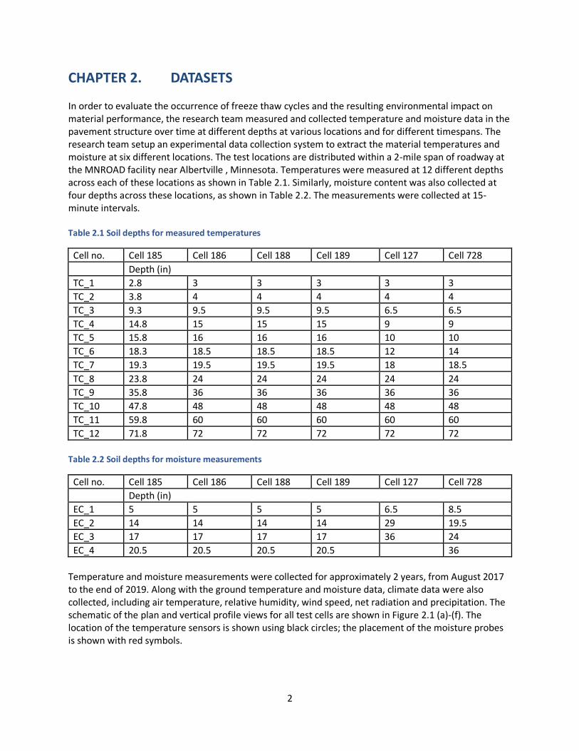
CHAPTER 2. DATASETS In order to evaluate the occurrence of freeze thaw cycles and the resulting environmental impact on material performance, the research team measured and collected temperature and moisture data in the pavement structure over time at different depths at various locations and for different timespans. The research team setup an experimental data collection system to extract the material temperatures and moisture at six different locations. The test locations are distributed within a 2-mile span of roadway at the MNROAD facility near Albertville , Minnesota. Temperatures were measured at 12 different depths across each of these locations as shown in Table 2.1. Similarly, moisture content was also collected at four depths across these locations, as shown in Table 2.2. The measurements were collected at 15-minute intervals. Table 2.1 Soil depths for measured temperatures

Cell no. Cell 185 Cell 186 Cell 188 Cell 189 Cell 127 Cell 728

Depth (in)

TC_1 2.8 3 3 3 3 3

TC_2 3.8 4 4 4 4 4

TC_3 9.3 9.5 9.5 9.5 6.5 6.5

TC_4 14.8 15 15 15 9 9

TC_5 15.8 16 16 16 10 10

TC_6 18.3 18.5 18.5 18.5 12 14

TC_7 19.3 19.5 19.5 19.5 18 18.5

TC_8 23.8 24 24 24 24 24

TC_9 35.8 36 36 36 36 36

TC_10 47.8 48 48 48 48 48

TC_11 59.8 60 60 60 60 60

TC_12 71.8 72 72 72 72 72

Table 2.2 Soil depths for moisture measurements

Cell no. Cell 185 Cell 186 Cell 188 Cell 189 Cell 127 Cell 728

Depth (in)

EC_1 5 5 5 5 6.5 8.5

EC_2 14 14 14 14 29 19.5

EC_3 17 17 17 17 36 24

EC_4 20.5 20.5 20.5 20.5 36

Temperature and moisture measurements were collected for approximately 2 years, from August 2017 to the end of 2019. Along with the ground temperature and moisture data, climate data were also collected, including air temperature, relative humidity, wind speed, net radiation and precipitation. The schematic of the plan and vertical profile views for all test cells are shown in Figure 2.1 (a)-(f). The location of the temperature sensors is shown using black circles; the placement of the moisture probes is shown with red symbols.

3

(a) (b)

(c) (d)

(e) (f) Figure 2.1 Schematic of the soil layers for temperature and moisture data collection for the locations of (a) Cell 185; (b) Cell 186; (c) Cell 188; (d) Cell 189; (e) Cell 127; (f) Cell 728

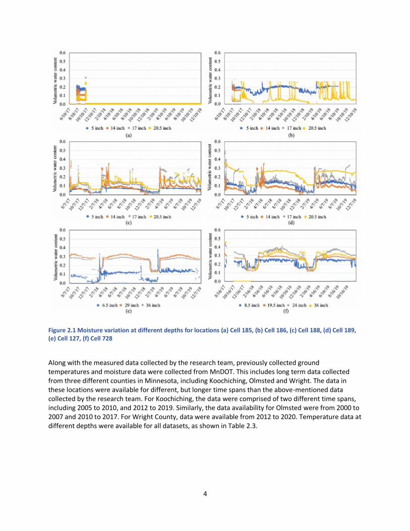
Moisture data for all test locations are also shown in Figure 2.2 (a-f). Apart from Cell 185, moisture data were collected across the entire data collection period at different depths. However, the moisture data were not as influential as the environmental parameters for the soil temperature prediction. Thus, they are not incorporated in this study

4

Figure 2.1 Moisture variation at different depths for locations (a) Cell 185, (b) Cell 186, (c) Cell 188, (d) Cell 189, (e) Cell 127, (f) Cell 728

Along with the measured data collected by the research team, previously collected ground temperatures and moisture data were collected from MnDOT. This includes long term data collected from three different counties in Minnesota, including Koochiching, Olmsted and Wright. The data in these locations were available for different, but longer time spans than the above-mentioned data collected by the research team. For Koochiching, the data were comprised of two different time spans, including 2005 to 2010, and 2012 to 2019. Similarly, the data availability for Olmsted were from 2000 to 2007 and 2010 to 2017. For Wright County, data were available from 2012 to 2020. Temperature data at different depths were available for all datasets, as shown in Table 2.3.

5

Table 2.3: Data availability for different locations

Dataset location Time span Depth of temperature sensor (in)

Koochiching

2005 to 2010 1; 4; 7; 9; 12; 18; 24; 30; 36; 42; 48; 54; 60; 72; 84; 96

2012 to 2019 1; 3; 5; 8; 12; 15; 18; 21; 24; 30; 36; 42; 48; 54; 60; 64; 78; 91

Olmsted

2000 to 2007 2.5; 6; 9; 12; 18; 24; 30; 36; 42; 48; 60; 72; 84; 96; 108

2010 to 2017 1; 2.5; 5; 7; 13; 19; 25; 31; 37; 43; 49; 55; 61; 73; 85; 97

Wright 2012 to 2020 0.5; 2; 3.5; 5; 12; 18; 24; 30; 36; 42; 48; 54; 60; 72; 84; 96

These three datasets were available for longer timespans. However, the data were collected at 1-hour time intervals rather than 15-minute intervals. Both sets of data were used in this study since the use of both sets of data were beneficial for model development and evaluation. Next, the raw data from the above-mentioned datasets were subjected to quality control prior to use in model development. For each location, the number of missing elements were counted for all the depths separately; the percent of missing elements are shown in Table 2.4 and Table 2.5. Table 2.4: Percentage of missing elements in the collected dataset in the MnROAD Test Cells

TC1 TC2 TC3 TC4 TC5 TC6 TC7 TC8 TC9 TC10 TC11 TC12

Cell 185 2 2 2 2 2 2 2 2 12 2 87 2

Cell 186 < 1 < 1 < 1 < 1 < 1 < 1 < 1 < 1 11 < 1 < 1 < 1

Cell 188 < 1 < 1 0 0 0 0 0 0 0 0 0 0

Cell 189 < 1 < 1 0 0 0 0 0 0 NA 0 0 0

Cell 127 < 1 < 1 < 1 < 1 < 1 < 1 < 1 < 1 < 1 < 1 < 1 < 1

Cell 728 < 1 < 1 < 1 0 0 0 0 0 0 0 0 0

*Note: NA: No data is available

6

Table 2.5: Percentage of missing elements in the MNDOT collected dataset

Location Timespan Percentage of missing elements

Koochiching

2005-2010

TC1 TC2 TC3 TC4 TC5 TC6 TC7 TC8 TC9

< 1 < 1 < 1 < 1 58 < 1 < 1 < 1 < 1


< 1 < 1 < 1 < 1 < 1 < 1 < 1 4 5

2012-2019


54 50 41 < 1 < 1 < 1 < 1 < 1 < 1


< 1 < 1 < 1 < 1 < 1 < 1 < 1 < 1 < 1

Olmsted

2000-2007


7 7 7 7 7 28 7 7 7

TC10 TC11 TC12 TC13 TC14 TC15

7 7 9 7 7 7

2010-2017


< 1 < 1 < 1 < 1 58 < 1 < 1 < 1 < 1

TC10 TC11 TC12 TC13 TC14 TC15 TC16

< 1 < 1 < 1 < 1 58 < 1 < 1

Wright

2012-2020


30 < 1 < 1 < 1 < 1 < 1 < 1 < 1 < 1

TC10 TC11 TC12 TC13 TC14 TC15 TC16

< 1 46 < 1 < 1 < 1 < 1 < 1

After removing the missing elements, outliers were identified and removed. If more than 40% data were missing, those datasets were not used for further analysis. Forward imputation (Barnard et al., 1999, Solaro et al., 2017), which is a sequential procedure to fill up the missing data in a step-by-step process by exploiting the data structure and interconnections among variable, was then used to fill in the missing elements.

7

CHAPTER 3. CALCULATION OF FREEZE-THAW CYCLES The occurrence of freeze-thaw cycles significantly impacts the performance of pavement systems over time. Thus, one of the objectives of this study is to evaluate the number of freeze thaw cycles occurring at different soil depths based on measured data. However, there is no widely accepted method to calculate the number of freeze-thaw cycles from soil temperature data. Freeze-thaw cycles consist of two components, including a freezing component and a thawing component (Figure 3.1). One freeze-thaw cycle must include both in sequential order. To ensure complete freezing, the soil temperature needs to be lower than the freezing point temperature, and after it must be higher than the thaw temperature to ensure the soil is completely thawed (MnDOT, 2014). Thus the number of freeze-thaw cycles depend on the freezing and thawing temperature and time duration needed to ensure freezing and thawing for soils at different depths. To evaluate the number of cycles, several different methods were assessed, as follows.

Figure 3.1 Freeze-thaw cycle diagram

3.1. FIXED FREEZING TEMPERATURE

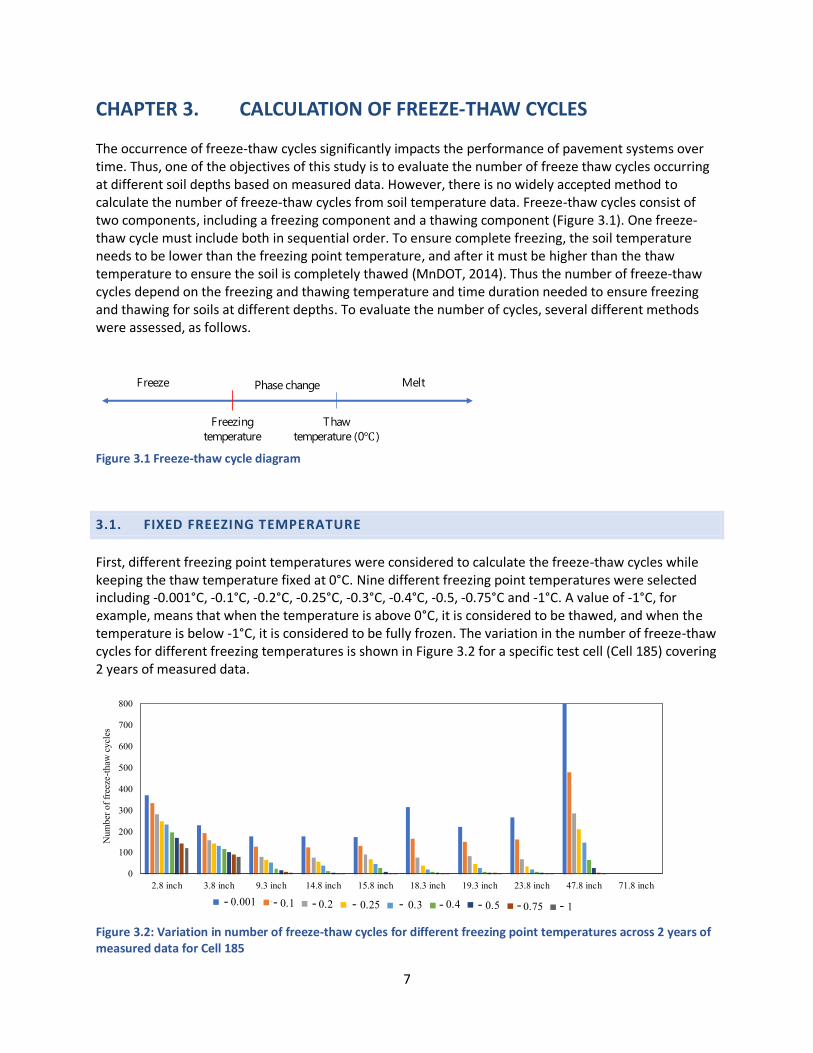
First, different freezing point temperatures were considered to calculate the freeze-thaw cycles while keeping the thaw temperature fixed at 0°C. Nine different freezing point temperatures were selected including -0.001°C, -0.1°C, -0.2°C, -0.25°C, -0.3°C, -0.4°C, -0.5, -0.75°C and -1°C. A value of -1°C, for example, means that when the temperature is above 0°C, it is considered to be thawed, and when the temperature is below -1°C, it is considered to be fully frozen. The variation in the number of freeze-thaw cycles for different freezing temperatures is shown in Figure 3.2 for a specific test cell (Cell 185) covering 2 years of measured data.

Figure 3.2: Variation in number of freeze-thaw cycles for different freezing point temperatures across 2 years of measured data for Cell 185

Freezing

temperature

Thaw

temperature (0℃ )

MeltFreeze Phase change

0

100

200

300

400

500

600

700

800

2.8 inch 3.8 inch 9.3 inch 14.8 inch 15.8 inch 18.3 inch 19.3 inch 23.8 inch 47.8 inch 71.8 inch

Num

ber

of

free

ze-t

haw

cycl

es

0.001 0.1 0.2 0.25 0.3 0.4 0.5 0.75 1

0

100

200

300

400

500

600

700

800


Nu

mb

er o

f fr

eeze

-th

aw c

ycl

es

0.001 0.1 0.2 0.25 0.3 0.4 0.5 0.75 1

0

100

200

300

400

500

600

700

800


Nu

mb

er o

f fr

eeze

-th

aw c

ycl

es

0.001 0.1 0.2 0.25 0.3 0.4 0.5 0.75 1

0

100

200

300

400

500

600

700

800


Nu

mb

er o

f fr

eeze

-th

aw c

ycl

es

0.001 0.1 0.2 0.25 0.3 0.4 0.5 0.75 1

0

100

200

300

400

500

600

700

800


Nu

mb

er o

f fr

eeze

-th

aw c

ycl

es

0.001 0.1 0.2 0.25 0.3 0.4 0.5 0.75 1

0

100

200

300

400

500

600

700

800


Nu

mb

er o

f fr

eeze

-th

aw c

ycl

es

0.001 0.1 0.2 0.25 0.3 0.4 0.5 0.75 1

0

100

200

300

400

500

600

700

800


Nu

mb

er o

f fr

eeze

-th

aw c

ycl

es

0.001 0.1 0.2 0.25 0.3 0.4 0.5 0.75 1

0

100

200

300

400

500

600

700

800


Nu

mb

er o

f fr

eeze

-th

aw c

ycl

es

0.001 0.1 0.2 0.25 0.3 0.4 0.5 0.75 1

0

100

200

300

400

500

600

700

800


Nu

mb

er o

f fr

eeze

-th

aw c

ycl

es

0.001 0.1 0.2 0.25 0.3 0.4 0.5 0.75 1

0

100

200

300

400

500

600

700

800


Nu

mb

er o

f fr

eeze

-th

aw c

ycl

es

0.001 0.1 0.2 0.25 0.3 0.4 0.5 0.75 1

0

100

200

300

400

500

600

700

800


Nu

mb

er

of

freeze-t

haw

cy

cle

s

0.001 0.1 0.2 0.25 0.3 0.4 0.5 0.75 1- - - - - - - - -

8

As seen in Figure 3.2, for freezing point temperatures closer to the thaw temperature, the number of freeze-thaw cycles for Cell 185 increases significantly. In addition, for these freezing point temperatures, the number of freeze-thaw cycles increases with increasing depth (Zegeye et al., 2019). The reason that this occurs is that, at the deeper locations, the fluctuations in the temperatures are much lower than the shallower depths, thus if at the deeper locations, the temperatures fluctuation is around 0°C (e.g. at the 48 in depth in Figure 3.2), A significant increase in the count of freeze-thaw cycles can be seen when the freezing point temperatures are closest to 0°C. This requires careful consideration. Given that the accuracy of the temperature sensors used to collect the data is +/- 1°C, it is recommended to consider -1°C freezing point temperature to calculate the number of freeze-thaw cycles. To assess the similarity of these counts of freeze-thaw cycles in literature, the resulting number of freeze-thaw cycles from the above-mentioned analysis was compared with a similar study where the data were collected from various locations in the state of Minnesota (MnDOT, 2014). In that study, the average number of freeze-thaw cycles across a 10-year period was evaluated at a depth of one inch below the surface, as shown in Figure 3.3. A freezing point temperature of 0°C was used in the study. As shown in Figure 3.3, an average of 86 cycles was found across the months of October to April.

Figure 3.3: Average freeze-thaw cycles by month from a prior MnDOT study (MnDOT, 2014)

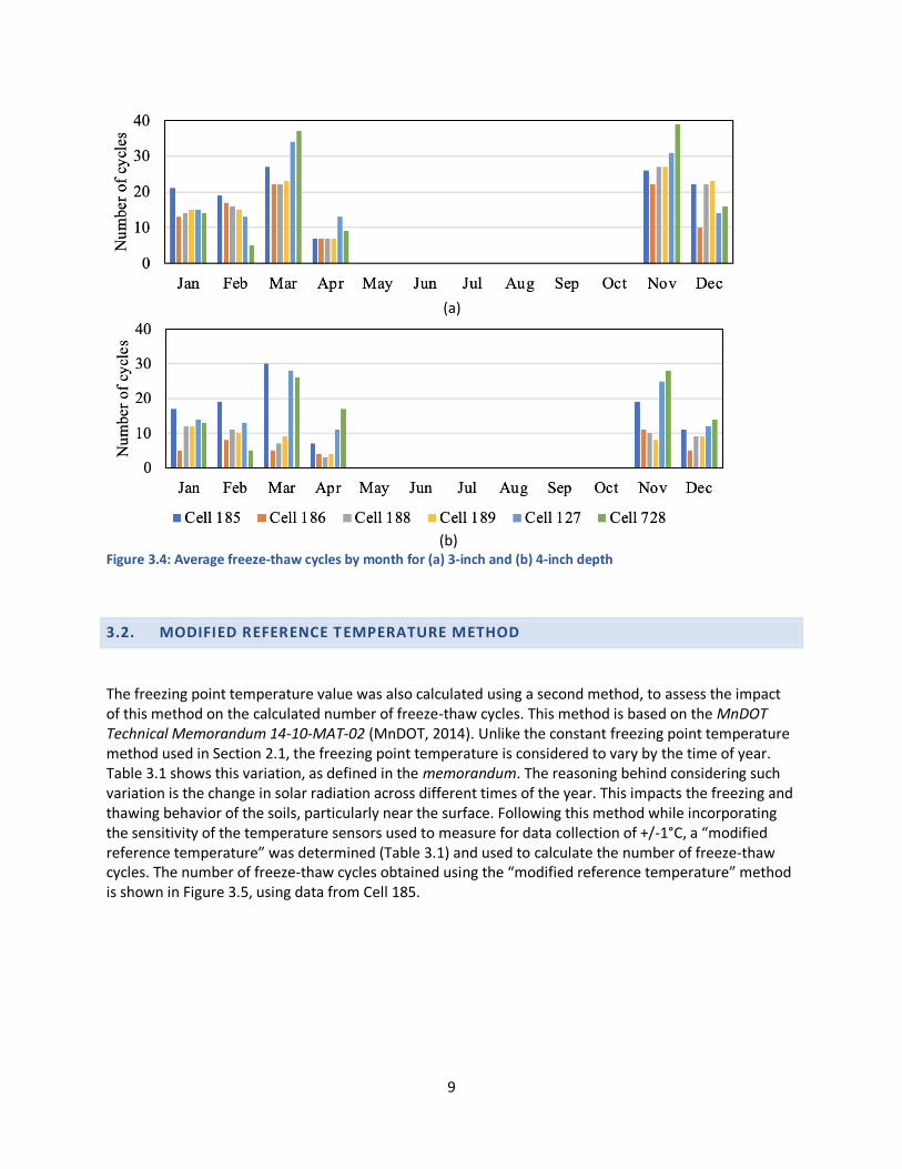
In the present study, based on the measured data, a similar analysis was performed. A freezing point temperature of -1°C was used to incorporate the sensitivity of the sensors. The number of freeze-thaw cycles for the 3- and 4-inch depths in different test cells is shown in Figure 3.4a and 3.4b for the same months as the study represented in Figure 3.3. As shown in Figure 3.4, the number of cycles calculated in this study decreases with increasing depth from the surface. Similar to the previous study and Figure 3.3, the number of cycles is higher for the month of March at the end of winter, and during November, and at the start of the winter season.

9

(a)

(b) Figure 3.4: Average freeze-thaw cycles by month for (a) 3-inch and (b) 4-inch depth

3.2. MODIFIED REFERENCE T EMPERATURE METHOD

The freezing point temperature value was also calculated using a second method, to assess the impact of this method on the calculated number of freeze-thaw cycles. This method is based on the MnDOT Technical Memorandum 14-10-MAT-02 (MnDOT, 2014). Unlike the constant freezing point temperature method used in Section 2.1, the freezing point temperature is considered to vary by the time of year. Table 3.1 shows this variation, as defined in the memorandum. The reasoning behind considering such variation is the change in solar radiation across different times of the year. This impacts the freezing and thawing behavior of the soils, particularly near the surface. Following this method while incorporating the sensitivity of the temperature sensors used to measure for data collection of +/-1°C, a “modified reference temperature” was determined (Table 3.1) and used to calculate the number of freeze-thaw cycles. The number of freeze-thaw cycles obtained using the “modified reference temperature” method is shown in Figure 3.5, using data from Cell 185.

10

Table 3.1. Reference temperature variation as defined by MnDOT Technical Memorandum 14-10-MAT-02 and modified reference temperature by time of year

Date Reference temperature (°C) Modified reference temperature (°C)

January 1- January 31 0 -1.0

February 1- February 7 -1.5 -1.5




March 1 – March 7 -3.5 -3.5

March 8 – March 14 -4.0 -4.0

March 15 – March 21 -4.5 -4.5

March 22 – March 28 -5.0 -5.0

March 29 – April 4 -5.5 -5.5

April 5 - April 11 -6.0 -6.0

April 12 - April 18 -6.5 -6.5

April 19 - April 25 -7.0 -7.0

April 26 – May 2 -7.5 -7.5

May 3- May 9 -8.0 -8.0

May 10- May 16 -8.5 -8.5

May 10- May 23 -9.0 -9.0

May 24- May 30 -9.5 -9.5

June 1- December 31 0 -1.0

Figure 3.5: Number of freeze-thaw cycles obtained using modified reference temperature method for Cell 185

3.3. TIME DELAY METHOD

Another method considered in this effort includes the incorporation of a “time delay” for the purposes of ensuring that complete freezing and thawing has occurred in the studied soils. A “time delay” is defined as a minimum period of time required for a half of a freeze-thaw cycle to be completed. For

0

2

4

6

8

10

12

14

16

18


Nu

mber

of

free

ze-t

haw

cycl

es

11

example, a “time delay” of 1 hour indicates that for at least 1 hour, the studied soil must be below the freezing point temperature. An example soil temperature distribution for a single day is shown in Figure 3.6 which demonstrates the time delay concept for complete freezing. If the period of time below the freezing point temperature is less than 1 hour, that portion of the freeze-thaw cycle is not considered to have occurred. To complete a freeze-thaw cycle, the soil temperature needs to be higher than the thawing temperature for the time delay period to ensure complete thawing.

Figure 3.6: Schematic of the time delay scenario to calculate the number of freeze-thaw cycles

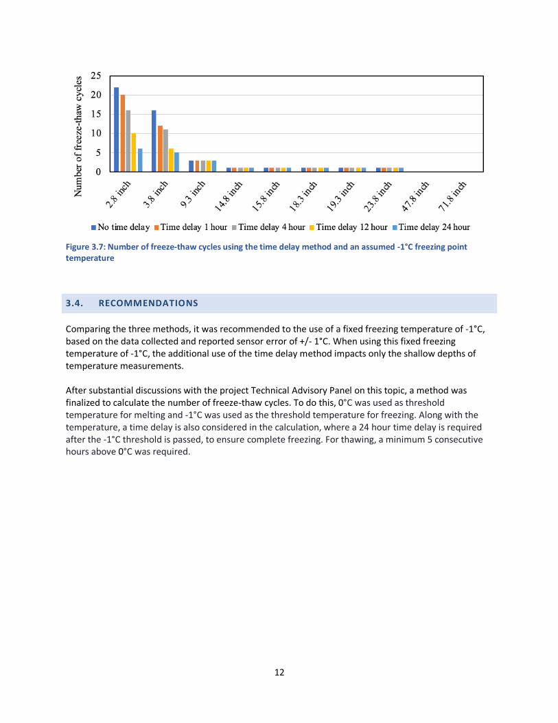
Similarly, the soil temperature must be lower than the freezing point temperature for the designated time period to ensure complete freezing. Different time delays were considered, from 0 to 24 hours, the results of which are shown in Figure 3.7.

12

Figure 3.7: Number of freeze-thaw cycles using the time delay method and an assumed -1°C freezing point temperature

3.4. RECOMMENDATIONS

Comparing the three methods, it was recommended to the use of a fixed freezing temperature of -1°C, based on the data collected and reported sensor error of +/- 1°C. When using this fixed freezing temperature of -1°C, the additional use of the time delay method impacts only the shallow depths of temperature measurements. After substantial discussions with the project Technical Advisory Panel on this topic, a method was finalized to calculate the number of freeze-thaw cycles. To do this, 0°C was used as threshold temperature for melting and -1°C was used as the threshold temperature for freezing. Along with the temperature, a time delay is also considered in the calculation, where a 24 hour time delay is required after the -1°C threshold is passed, to ensure complete freezing. For thawing, a minimum 5 consecutive hours above 0°C was required.

13

CHAPTER 4. MODEL DEVELOPMENT

4.1. DATA PROCESSING

Two different datasets were used in this study. For ease and clarity of discussion, the datasets were named as Dataset 1 and Dataset 2. Along with the soil temperatures at different depths, climate data were in Dataset 1. These data were collected across a 2-mile span of roadway in MNROAD facility near Albertville , Minnesota. Air temperature, relative humidity, wind speed, precipitation and solar radiation data were collected at a 15-minute timestep to be consistent with the collected temperature data granularity. In Dataset 2, soil temperature data were collected at a 1-hour time interval in three different counties in Minnesota, including Koochiching, Olmsted and Wright. For brevity, the focus was on the data collected in Olmsted county in this section, as data timespan of the three locations are similar. The climatic variables were pre-processed to create a list of potential variables which can be used as the input parameters in the modeling process. The final list of parameters considered can be divided in two categories: time variables and climate variables. The list of all the variables is shown below: The time variables considered include: 1. Month number (1 to 12) 2. Week number (1 to 52) 3. Day of year (1 to 365) 4. Timestep (1 to 4*24 for 15-minute timestep data) The climatic variables considered include: 1. Air temperature (AirTemp) 2. Relative humidity (RH) 3. Rain or precipitation (Rain) 4. Windspeed (Wind) 5. Radiation (Rad) 6. Daily average air temperature (avgTemp) 7. Daily average relative humidity (avgRH) 8. Daily average precipitation (avgRain) 9. Daily average windspeed (avgWind) 10. Daily average solar radiation (avgrad) 11. Variation of the air temperature with respect to the daily average value (varTemp) 12. Variation of the relative humidity with respect to the daily average value (varRH) 13. Variation of the precipitation with respect to the daily average value (varRain) 14. Variation of the windspeed with respect to the daily average value (varWind) 15. Variation of the solar radiation with respect to the daily average value (varRad) The variation values were calculated by subtracting the daily average values from the instantaneous value at a specific time interval, using the following: Variation = Instantaneous value – Average value of a specific day

14

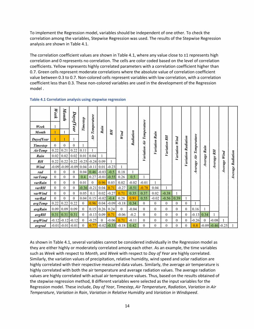
To implement the Regression model, variables should be independent of one other. To check the correlation among the variables, Stepwise Regression was used. The results of the Stepwise Regression analysis are shown in Table 4.1. The correlation coefficient values are shown in Table 4.1, where any value close to ±1 represents high correlation and 0 represents no correlation. The cells are color coded based on the level of correlation coefficients. Yellow represents highly correlated parameters with a correlation coefficient higher than 0.7. Green cells represent moderate correlations where the absolute value of correlation coefficient value between 0.3 to 0.7. Non-colored cells represent variables with low correlation, with a correlation coefficient less than 0.3. These non-colored variables are used in the development of the Regression model . Table 4.1 Correlation analysis using stepwise regression

Tim

este

p

Air

Tem

per

atu

re

Rain

RH

Win

d

Radia

tion

Vari

ati

on

Air

Tem

per

atu

re

Vari

ati

on

Rain

Vari

ati

on

RH

Vari

ati

on

Win

d

Vari

ati

on

Radia

tion

Ave

rage

Air

Tem

per

atu

re

Ave

rage

Rain

Ave

rage

RH

Ave

rage

Win

d

Ave

rage

Radia

tion

Week 1

Month 1 1

DayofYear 1 1 1

Timestep 0 0 0 1

AirTemp 0.22 0.21 0.22 0.11 1

Rain 0.02 0.02 0.02 0.01 0.04 1

RH 0.22 0.22 0.22 -0.25 -0.24 0.09 1

Wind -0.09 -0.09 -0.09 0.04 -0.11 0.01 -0.23 1

rad 0 0 0 0.04 0.46 -0.03 -0.5 0.18 1

varTemp 0 0 0 0.4 0.27 -0.01 -0.55 0.26 0.5 1

varRain 0 0 0 0.01 0 0.96 0.03 0.02 -0.02 -0.01 1

varRH 0 0 0 -0.36 -0.21 0.04 0.71 -0.27 -0.51 -0.78 0.04 1

varWind 0 0 0 0.05 0.1 0.02 -0.27 0.71 0.35 0.37 0.02 -0.38 1

varRad 0 0 0 0.04 0.15 -0.02 -0.4 0.28 0.91 0.55 -0.02 -0.56 0.39 1

avgTemp 0.22 0.22 0.22 0 0.96 0.04 -0.09 -0.18 0.34 0 0 0 0 0 1

avgRain 0.09 0.09 0.09 0 0.15 0.26 0.24 0 -0.04 0 0 0 0 0 0.16 1

avgRH 0.31 0.31 0.31 0 -0.13 0.09 0.71 -0.06 -0.2 0 0 0 0 0 -0.13 0.34 1

avgWind -0.12 -0.12 -0.12 0 -0.25 0 -0.06 0.71 -0.11 0 0 0 0 0 -0.26 0 -0.08 1

avgrad -0.01 -0.01 -0.01 0 0.77 -0.02 -0.33 -0.18 0.42 0 0 0 0 0 0.8 -0.09 -0.46 -0.25 1

As shown in Table 4.1, several variables cannot be considered individually in the Regression model as they are either highly or moderately correlated among each other. As an example, the time variables such as Week with respect to Month, and Week with respect to Day of Year are highly correlated. Similarly, the variation values of precipitation, relative humidity, wind speed and solar radiation are highly correlated with their respective measured data values. Similarly, the average air temperature is highly correlated with both the air temperature and average radiation values. The average radiation values are highly correlated with actual air temperature values. Thus, based on the results obtained of the stepwise regression method, 8 different variables were selected as the input variables for the Regression model. These include, Day of Year, Timestep, Air Temperature, Radiation, Variation in Air Temperature, Variation in Rain, Variation in Relative Humidity and Variation in Windspeed.

Mo

nth

Week

Dayo

fYea

r

15

Dataset 1 and Dataset 2 were then used to create the data-driven models. Dataset 1, with approximately 1.5-2 years of data available at each cell (16 months) from January 1, 2018 to April 16, 2019, was split into two datasets, one for use in training the model, and a second for model testing. This split was a 75%-25% split where 12 months of data (2018) were used as training data, and January 1, 2019 to the end of the dataset were used for the testing of the model. For Dataset 2, with data across multiple years, data were split in an 80%-20% division, where 80% of it were used for the training purpose and the rest of the data were used as testing data. For example, for the Olmsted location, data from September 2005 to February 2007 were used as testing data and January 2000 to September 2005 were used at training data. The reason that the datasets were split slightly differently is because for Dataset 1, training dataset was selected to include one whole year and similarly for Dataset 2, the objective was to select an entire winter season for training data. For weather data, for Dataset 1, onsite field collected data were used; for Dataset 2, the nearest available weather station data were used for each location.

4.2. MODEL DEVELOPMENT

As mentioned, there are no well accepted algorithm that can be used for the prediction of the soil surface temperatures. At the initial stage of the study, different models were implemented to study which algorithm performs best. Initially, a Linear Regression model was used, followed by Regression models used for time series data forecasting, including Vector Auto Regression, Vector Auto Regression Moving Average, and Vector Error Correction Models. However, the above-mentioned models were unable to accurately capture the granular trend in soil temperature. An example result of soil temperature prediction is shown in Figure 4.1. This was obtained for a specific cell location and at a specific depth using Vector Auto Regression modeling methods. The results show the predicted temperature for testing dataset where x-axis of the figure shows timestep of the year. However, the results obtained for the other mentioned algorithms were also similar for all the soil depths. Thus, Nonlinear Regression models were implemented, and the performance of the soil temperature prediction improved significantly using this method.

16

Figure 4.1. Temperature prediction using Vector Auto Regression Model

4.2.1. Temperature prediction

A Nonlinear Regression modeling method was implemented using a fourth order polynomial model. Two modeling methods were considered based on a Nonlinear Regression algorithm. Model 1 predicts temperature at each depth individually, using a single model. Two time variables and six climate variables were used as input. These include Day of Year, Timestep, Air Temperature, Radiation, Variation in Air Temperature, Variation in Rain, Variation in Relative Humidity and Variation in Windspeed. The equation for the Model 1 is in Appendix Table A 1. Model 2 was developed using a combination of two parts - one to predict the daily average soil temperatures, and a second to predict the variation in soil temperature with respect to the daily average values. To predict the daily average soil temperatures, six variables were used (Day of Year, Timestep, Average Air Temperature, Average Rain, Average Relative Humidity and Average Wind Speed. For the second half of the model, Day of Year, Timestep, Air Temperature, Radiation, Variation in Air Temperature, Variation in Rain, Variation in Relative Humidity and Variation in Wind Speed were used as the input parameters. The results of the soil temperature prediction are shown in Figure 4.2 for both initial models, including the temperature at three depths (3-inch, 14-inch, 72-inch). These three depths were selected to be presented because they represent the top surface (largest diurnal fluctuations), intermediate depth, and deep depth (least fluctuations). The timespan of the temperature prediction shown in Figure 4.2 is for 4 months of data from January 2019 to April 2019, which represents the second part of winter. This time span is used because January to December 2018 was used as training data, thus the remaining 4 months was used as testing data. This divides the dataset in a 75%-25% split where 75% of the data were used for training and rest 25% were used for testing. The Models are labeled as “initial” models in Figure 4.2 because further adjustments were made to the modeling method to arrive at the final Models for this work.

17

Figure 4.2. Comparison between the measured and predicted temperature for depths of (a) 3 inch, (b) 14 inch and (c) 72 inch below the surface for the initial Model 1 and Model 2 for the timeframe of January to April

As shown, the temperature fluctuations at the top surface are greater, whereas this fluctuation decreases with depth, as expected. Both the Models can predict the temperature at the top surface quite well. However, the performance of these initial Models reduces at deeper depths. At a depth of 14-inch, Model 2 predicts the overall trend of the temperature for most of the timespan. However, several spikes occur where the predicted temperature deviates significantly compared to the measured temperature data. Model 1 did not generate any spikes in the temperature prediction. However, the predicted temperature deviates from the measured soil temperature more than Model 2. To reduce the spikes in the model predictions, two different filters were used. The objective of the filters was to limit the allowable variation in the model results from timestep (n-1) to the next timestep (n). In addition, the filters were also designed to limit temperature predictions which were significantly higher or lower than the measured temperature bounds (i.e. the minimum and maximum soil temperatures observed for each depth throughout the dataset). To identify the temperature bounds, the range of soil temperatures (maximum and minimum) expected for each depth across the dataset was assessed. The RMSE (root mean squared error) values for both the initial Models and the models which include the developed filters for all six locations at the MNROAD test facility and several depths are shown in Figure 4.3. A smaller RMSE values equates to better model performance over the timespan of evaluation.

18

Figure 4.3. Comparison of RMSE values for initial Model 1 and 2, and Model 1 and 2 with filters applied, at depths of (a) 3 inches, (b) 4 inches, (c) 18.5 inches, (d) 24 inches, (e) 48 inches and (f) 72 inches for all cell locations for Dataset 1

The results show that, overall, across the models, the RMSE values for predicting the soil temperature decrease at deeper depths. In addition, in comparing the models, Model 1 generally has larger error than Model 2. The use of the filters helps to reduce this model error. For 3-inch and 4-inch depths, RMSE values for Model 1 without the filters was approximately 8 to 12°C. After implementing both filters, the RMSE values were reduced to half, or approximately 4 to 6 °C. Model 2 has a significantly smaller RMSE values of 2 to 4°C with the use of filtering. For intermediate and deeper depths, Model 2 with the filters had the smallest RMSE values among the 4 model variations evaluated for all the depths in all locations. For the deepest depths, the smallest RMSE values were approximately 1 to 2°C for 18.5- and 48-inch depths, and less than 1°C for the 72-inch depth. These results demonstrate that Model 2 with filters provides the best prediction of temperature among the modeling methods implemented. A similar study was conducted using Dataset 2 which was the longer timescale data collected throughout Minnesota with a 1-hour timestep. The performance of both initial Model 1 and 2, and Model 1 and 2 with filters were evaluated for a time period starting from January 2000 to February 2007. This is substantially longer time period than the Dataset 1. The performance of both Model 1, Model 2 and the two models with filters are shown in Figure 4.4. As shown in the Figure, the RMSE values decreased at deeper depths as obtained for Dataset 1. However, the RMSE values were higher for this dataset compared to the model performance with previous set of data. The reason for these higher RMSE may be because the weather data used for model prediction was not collected on site and instead were obtained from the closest available weather station.

19

Figure 4.4: Comparison of RMSE values for Dataset 2

Based on the resulting performance of the models considered, the Model 2 with filters performed best in predicted temperatures at the various depths.

4.2.2. Prediction of number of freeze-thaw cycles

Based on the above-mentioned method for defining a freeze-thaw cycle (Section 3.4), the number of freeze-thaw cycles was evaluated from Dataset 1 using the four considered modeling methods, and compared with the number of cycles obtained from measured soil temperature (Figure 4.5). This figure also depicts the freeze-thaw cycle comparison for 4 months in the beginning of 2019 which represents the end of the winter. As discussed above, the reason this time period was used for this dataset is because for training one whole year of data were utilized, and the rest of the data were used as testing dataset. As shown in Figure 4.5, the number of freeze-thaw cycles obtained from the Model 1 is similar to the number of freeze-thaw cycles obtained from the measured data. At deeper depths, the number of freeze-thaw cycles decreased, as expected. Model 2 generally slightly overpredicts the number of cycles for most soil depths and locations, as compared to Model 1. The number of freeze-thaw cycles was also calculated for the Dataset 2, as shown in Figure 4.6.

20

Figure 4.5. Comparison of the freeze-thaw cycle variations for the four Models

21

Figure 4.6. Number of freeze-thaw cycle comparison for Dataset 2

As shown in Figure 4.6, apart from the 30-inch and 36-inch depths, the number of freeze-thaw cycles predicted by the Model 1 is similar to the actual number of freeze-thaw cycles. However, for the two mentioned depths, Model 1 and 2 overpredict the number of cycles. One possible reason for this is that, as mentioned in the previous section, the location of soil temperature collection and location of weather data were not same, which may impact the level of error in the input data. This result was consistent with the results obtained with the Dataset 1. Thus, from these two sections, it can be concluded that the Model 1 with 2 filters, is better suited to evaluate the number of freeze-thaw cycles effectively and thus is chosen as the final model for this project.

4.2.3. Isotherm calculation

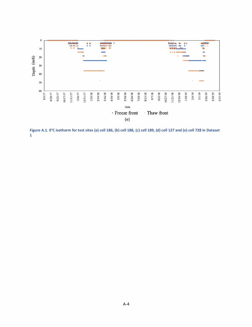
The distribution of the 0°C isotherm for different depths and different time periods were calculated from the measured data. The results of cell 185 are shown in Figure 4.7. The remaining figures are shown in Appendix A. The 0°C isotherm curve reaches its maximum depth during the months of December to February and then the depth of the isotherm curve reduces. A similar trend can be seen for all cell locations.

22

Figure 4.7. 0°C isotherm for cell 185 in Dataset 1

4.2.4. Time duration of freezing and thawing phase and their occurrence

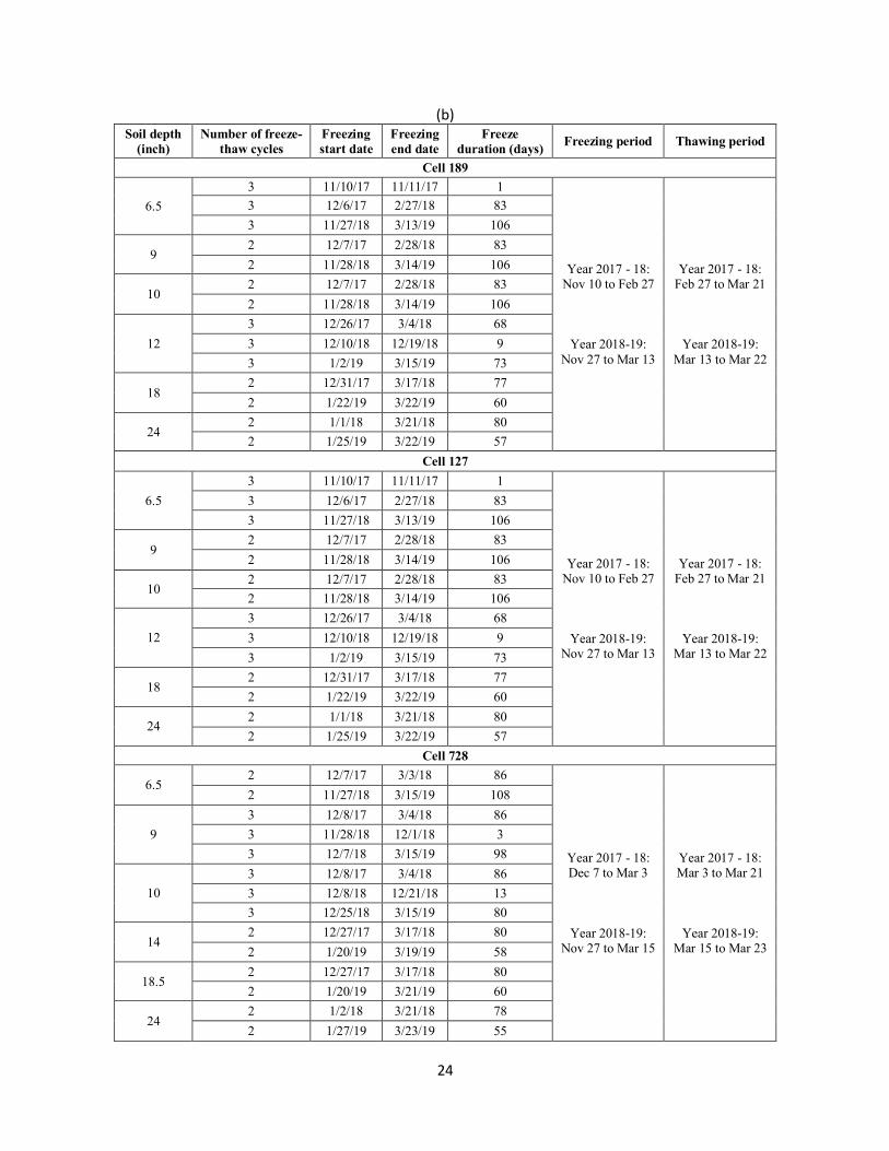
The duration of the frozen period including the start and end dates, was calculated for each soil depth along with the freezing and thawing periods for each test location. Using Dataset 1, these were evaluated for approximately 18 months of data, from September 2017 to April 2019 and shown in Table 4.2. It was obtained that for some years, for shallower depths, such as 6.5 inch in both Cell 189 and 127, the soil froze intermittently, in some cases for as little as 1-day periods. As expected, for deeper depths the temperatures fluctuate less thus there are not short freeze periods at these depths. The starting and ending time of freezing phase and their duration was compared for the predicted soil temperatures with the actual values. The performance of both the Model 1 and Model 2 were evaluated, as shown in Table 4.2. Model 1 performed significantly better compared to the Model 2. The performance of the Model 1 and its comparison with respect to the actual values is shown in Table 4.3. Note the freeze and thaw periods calculated for these cells assume the use of the shallowest soil depth that is not within the pavement foundation layers (i.e. base, subbase and subgrade layer) (e.g. cell 189 uses a soil depth of 6.5 in to calculate when the freezing and thawing period starts and ends).

23

Soil depth

(inch)

Number of freeze-

thaw cycles

Freezing start

date

Freezing end

date

Freeze duration

(days) Freezing period Thawing period

Cell 185

9.5 2 12/7/17 2/27/18 82

Year 2017 - 18: Dec 7 to Feb 27

Year 2018-19: Dec 7 to Mar 11

Year 2017 - 18: Feb 27 to Mar 20

Year 2018-19: Mar 11 to Mar 20

2 12/7/18 3/11/19 94

14.8 2 12/25/17 3/3/18 68

2 1/2/19 3/15/19 72

15.8 2 12/26/17 3/3/18 67

2 1/3/19 3/16/19 72

18.3 2 12/26/17 3/4/18 68

2 1/19/19 3/18/19 58

19.3 2 12/27/17 3/4/18 67

2 1/20/19 3/18/19 57

23.8 2 12/28/17 3/10/18 72

2 1/22/19 3/20/19 57

Cell 186

9.5

3 12/13/17 3/1/18 78

Year 2017 -18: Dec 13 to Mar 1


Year 2017 - 18: Mar 1 to Mar 12


3 12/7/18 12/22/18 15

3 12/30/18 3/14/19 74

15 2 12/26/17 3/4/18 68

2 1/1/19 3/17/19 74

16 2 12/26/17 3/4/18 68

2 1/3/19 3/17/19 73

18.5 2 12/27/17 3/7/18 70

2 1/21/19 3/19/19 57

19.5 2 12/28/17 3/7/18 69

2 1/21/19 3/19/19 57

24 2 12/31/17 3/12/19 71

2 1/26/19 3/21/19 54

Cell 188

9.5 2 12/12/17 2/28/18 78

Year 2017 - 18: Dec 13 to Mar 1


Year 2017 - 18: Mar 1 to Mar 15

Year 2018-19: Mar 15 to Apr 1

2 12/8/18 3/15/19 97

15 2 12/24/17 3/4/18 70

2 12/11/18 3/18/19 97

16 2 12/24/17 3/5/18 71

2 12/30/18 3/18/19 78

18.5 2 1/7/18 3/9/18 74

2 1/2/19 3/19/19 76

19.5 2 12/26/17 3/9/18 73

2 1/2/19 3/19/19 76

24 2 12/27/17 3/12/18 75

2 1/3/19 3/20/19 76

48 2 1/19/18 3/14/18 54

2 2/6/19 3/29/19 41

Table 4.2. Freezing start and end day with the duration for different soil depths for the location of (a) cell 185, (b) cell 186, (c) cell 188, (d) cell 189, (e) cell 127, (f) cell 728

(a)

24

(b) Soil depth

(inch)

Number of freeze-

thaw cycles

Freezing

start date

Freezing

end date

Freeze

duration (days) Freezing period Thawing period

Cell 189

6.5

3 11/10/17 11/11/17 1

Year 2017 - 18: Nov 10 to Feb 27

Year 2018-19:

Nov 27 to Mar 13

Year 2017 - 18: Feb 27 to Mar 21

Year 2018-19:

Mar 13 to Mar 22

3 12/6/17 2/27/18 83

3 11/27/18 3/13/19 106

9 2 12/7/17 2/28/18 83

2 11/28/18 3/14/19 106

10 2 12/7/17 2/28/18 83

2 11/28/18 3/14/19 106

12

3 12/26/17 3/4/18 68

3 12/10/18 12/19/18 9

3 1/2/19 3/15/19 73

18 2 12/31/17 3/17/18 77

2 1/22/19 3/22/19 60

24 2 1/1/18 3/21/18 80

2 1/25/19 3/22/19 57

Cell 127

6.5

3 11/10/17 11/11/17 1

Year 2017 - 18: Nov 10 to Feb 27

Year 2018-19: Nov 27 to Mar 13

Year 2017 - 18: Feb 27 to Mar 21


3 12/6/17 2/27/18 83

3 11/27/18 3/13/19 106

9 2 12/7/17 2/28/18 83

2 11/28/18 3/14/19 106

10 2 12/7/17 2/28/18 83

2 11/28/18 3/14/19 106

12

3 12/26/17 3/4/18 68

3 12/10/18 12/19/18 9

3 1/2/19 3/15/19 73

18 2 12/31/17 3/17/18 77

2 1/22/19 3/22/19 60

24 2 1/1/18 3/21/18 80

2 1/25/19 3/22/19 57

Cell 728

6.5 2 12/7/17 3/3/18 86

Year 2017 - 18: Dec 7 to Mar 3

Year 2018-19: Nov 27 to Mar 15

Year 2017 - 18: Mar 3 to Mar 21


2 11/27/18 3/15/19 108

9

3 12/8/17 3/4/18 86

3 11/28/18 12/1/18 3

3 12/7/18 3/15/19 98

10

3 12/8/17 3/4/18 86

3 12/8/18 12/21/18 13

3 12/25/18 3/15/19 80

14 2 12/27/17 3/17/18 80

2 1/20/19 3/19/19 58

18.5 2 12/27/17 3/17/18 80

2 1/20/19 3/21/19 60

24 2 1/2/18 3/21/18 78

2 1/27/19 3/23/19 55

25

Table 4.3. Comparison of freezing time for actual and predicted soil temperatures for Dataset 1 for the location of (a) cell 185, (b) cell 186, (c) cell 188, (d) cell 189, (e) cell 127, (f) cell 728 (note: Method 1 refers to Model1)

(a)

Depths Method Number of

cycles

Freezing start

day

Freezing end

day

Freezing

duration

Total freezing

duration

Cell 185

9.5 inch

Actual value 1 Jan-02 Mar-08 65 65

Model 1 3

Jan-02 Jan-07 5

60 Jan-09 Feb-23 45

Feb-26 Mar-08 10

14.8 inch Actual value 1 Jan-02 Mar-15 72 72

Model 1 1 Jan-02 Mar-09 66 66


Model 1 1 Jan-02 Mar-09 66 66


Model 1 1 Jan-02 Mar-03 60 60

19.3 inch


Model 1 2 Jan-02 Jan-07 5

57 Jan-10 Mar-03 52

23.8 inch


Model 1 2 Jan-02 Jan-07 5

57 Jan-10 Mar-03 52

Cell 186

9.5 inch


Model 1 2 Jan-02 Feb-23 52

63 Feb-25 Mar-08 11

15 inch Actual value 1 Jan-02 Mar-19 76 76

Model 1 1 Jan-02 Mar-09 66 66


Model 1 1 Jan-02 Mar-09 66 66


Model 1 1 Jan-02 Mar-09 66 66


Model 1 1 Jan-02 Mar-09 66 66


Model 1 1 Jan-10 Mar-09 58 58

26

(b)


cycles

Freezing start

day

Freezing end

day

Freezing

duration

Total freezing

duration

Cell 188

9.5 inch Actual value 2

Jan-02 Jan-07 5 63

Jan-09 Mar-08 58

Model 1 1 Jan-02 Mar-08 65 65


Model 1 1 Jan-02 Mar-09 66 66


Model 1 1 Jan-02 Mar-09 66 66

18.5 inch


Model 1 1 Jan-02 Mar-09 66 66

19.5 inch


Model 1 1 Jan-02 Mar-09 66 66


Model 1 1 Jan-02 Mar-09 66 66

48 inch Actual value 1 Feb-16 Mar-29 41 41

Model 1 1 Jan-30 Mar-02 31 31

Cell 189


Model 1 1 Jan-02 Mar-08 65 65


Model 1 1 Jan-02 Mar-09 66 66


Model 1 1 Jan-02 Mar-09 66 66


Model 1 1 Jan-02 Mar-09 66 66


Model 1 1 Jan-02 Mar-09 66 66


Model 1 1 Jan-02 Mar-09 66 66

48 inch Actual value 1 Mar-06 Apr-01 26 26

Model 1 1 Jan-30 Feb-14 15 15

27

(c)


cycles

Freezing start

day

Freezing end

day Freezing duration

Total freezing

duration

Cell 127

6.5 inch

Actual value 2 2 7 5

63 9 67 58

Model 1 3

2 7 5

65 9 67 58

72 74 2

9 inch

Actual value 1 2 73 71 71

Model 1 3

2 7 5

65 9 67 58

72 74 2

10 inch


Model 1 3

2 7 5

65 9 67 58

72 74 2

12 inch


Model 1 2 2 68 66 70

70 74 4

18 inch Actual value 1 22 82 60 60

Model 1 1 10 69 59 59


Model 1 1 13 69 56 56

Cell 728

6.5 inch

Actual value 2 2 7 5

68 2 9 72 63

Model 1 2 2 7 5

70 2 9 74 65

9 inch


Model 1 2 2 7 5

70 2 9 74 65

10 inch


Model 1

3 2 7 5

68 3 9 68 59

3 70 74 4

14 inch


Model 1

3 2 6 4

67 3 10 69 59

3 70 74 4

18.5 inch


Model 1 2 2 5 3

62 2 10 69 59


Model 1 1 17 69 52 52

28

As shown in Table 4.3, Model 1 can generally predict the freezing start and end day and the duration of the freezing phase for the Dataset 1. The predicted freezing and thawing period using Model 1 and the measured data-derived results are compared in Table 4.4. It can be seen from Table 4.4 that the Model 1 can predict the freezing period accurately for most of the cell locations. However, it underpredicts the time for the thawing period. Table 4.4. Comparison of freezing and thawing period for all cell locations using Dataset 1

Cell

location

Freezing period Thawing period

Actual value Predicted Actual value Predicted

Cell 185 Jan 2 – Mar 8 Jan 2 – Mar 3 Mar 8 – Mar 20 Mar 3 – Mar 9



Cell 189 Jan 2 – Mar 9 Jan 2 – Feb 14 Mar 9 – Apr 1 Feb 14 – Mar 9



29

CHAPTER 5. TOOL DEVELOPMENT The focus of this task was to create an Excel-based modeling tool to predict the soil temperatures and number of freeze-thaw cycles for different soil depths. Excel was requested to be used for this tool as it is available to and commonly used by the target audience. This tool developed was achieved using Excel macro functions and VBA programs. It is noted that as Excel is used, there are more efficient methods (e.g. python) for tool execution, and that choice of Excel somewhat limits some of the speed of results output. However, it does achieve the desired functionality. This tool allows the user to provide climate condition data and the depth at which the soil temperature and freeze-thaw cycles are desired to be calculated. The tool then provides a prediction, for the given weather conditions, of the soil temperatures at that depth over time and the predicted number freeze-thaw cycles. The framework of the tool is designed in three layers, as shown in Figure 5.1.

Figure 5.1: Framework of the Excel-based tool

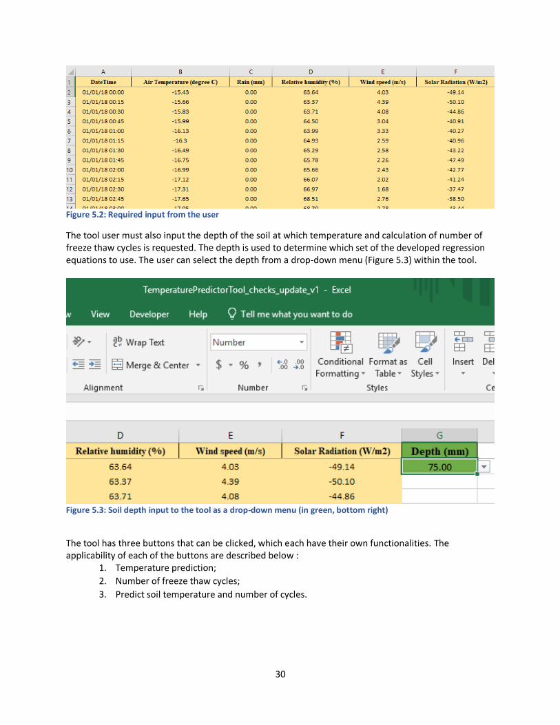
In (1) the first part, the tool requires the user to provide climate data for the location of interest. The following inputs are required at a frequency of 15 minutes in the following format:

1. Date and time in mm/dd/yy hh:mm

2. Air temperature in ⁰C

3. Precipitation in mm

4. Relative humidity in %

5. Windspeed in m/s

6. Net radiation in W/m2

As an example, of these values, the inputs of the tool should be in the format shown in Figure 5.2, as follows.

(1) Prediction of soil temperature

(2) Temperature filtration

(3) Calculation of the number of cycles

30

Figure 5.2: Required input from the user

The tool user must also input the depth of the soil at which temperature and calculation of number of freeze thaw cycles is requested. The depth is used to determine which set of the developed regression equations to use. The user can select the depth from a drop-down menu (Figure 5.3) within the tool.

Figure 5.3: Soil depth input to the tool as a drop-down menu (in green, bottom right)

The tool has three buttons that can be clicked, which each have their own functionalities. The applicability of each of the buttons are described below :

1. Temperature prediction;

2. Number of freeze thaw cycles;

3. Predict soil temperature and number of cycles.

31

5.1. TEMPERATURE PREDICTION

Based on the given input to the tool and after selecting the depth, choosing this button results in the temperature prediction for each timestep, as shown in Figure 5.4. Predicted temperatures will be added in the highlighted column AG.

Figure 5.4. Example results of the ‘Temperature prediction’ button

5.2. NUMBER OF FREEZE-THAW CYCLES

Based on the predicted temperature, this button calculates three values, as follows. Note that this button must be clicked on after the “temperature prediction” button. Figure 5.5 shows an example of the results in Columns L through O.

number of freeze-thaw cycles,

starting of freeze and thaw mode and

the duration of each of the freeze-thaw cycles

Figure 5.5. Example results of the ‘Number of freeze-thaw cycles prediction’ button

5.3. PREDICT SOIL TEMPERATURE AND NUMBER OF FREEZE-THAW CYCLES

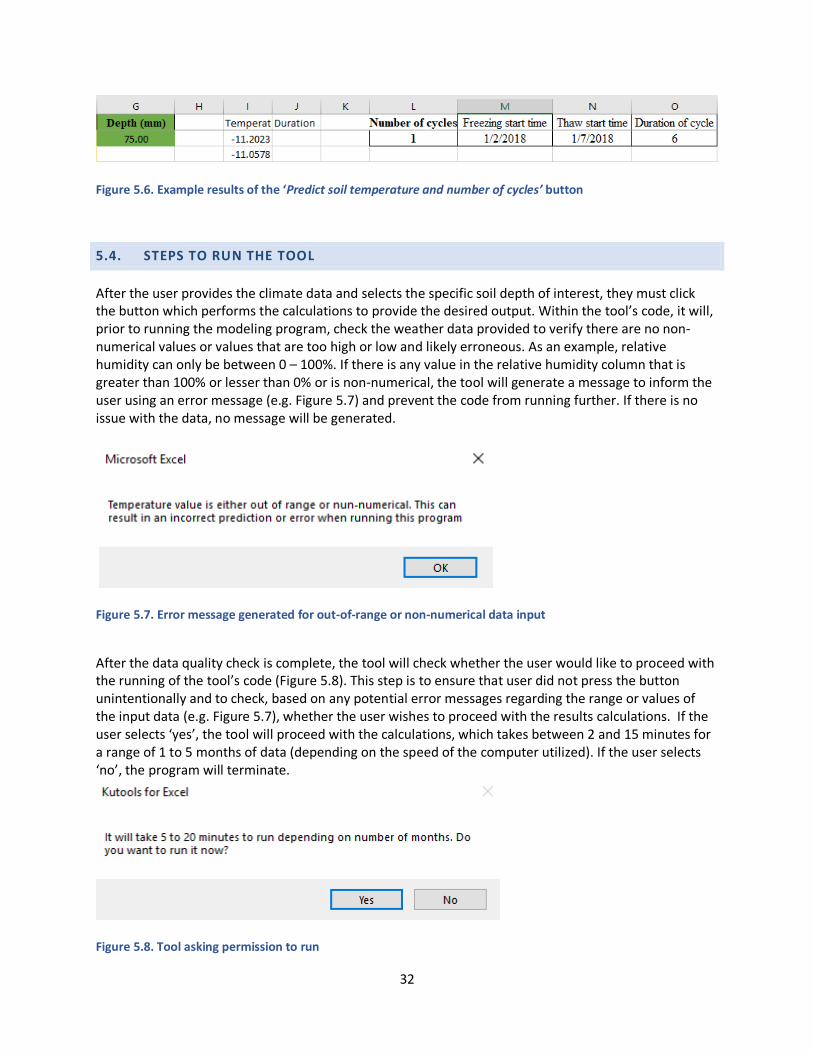
This button accomplishes what is done for button 1 and 2 in one step, and includes the temperature prediction, and the calculation of number of freeze-thaw cycles and their duration. The results would include a combination of Figure 5.4 and Figure 5.5, an example of which is shown in Figure 5.6.

32

Figure 5.6. Example results of the ‘Predict soil temperature and number of cycles’ button

5.4. STEPS TO RUN THE TOOL

After the user provides the climate data and selects the specific soil depth of interest, they must click the button which performs the calculations to provide the desired output. Within the tool’s code, it will, prior to running the modeling program, check the weather data provided to verify there are no non-numerical values or values that are too high or low and likely erroneous. As an example, relative humidity can only be between 0 – 100%. If there is any value in the relative humidity column that is greater than 100% or lesser than 0% or is non-numerical, the tool will generate a message to inform the user using an error message (e.g. Figure 5.7) and prevent the code from running further. If there is no issue with the data, no message will be generated.

Figure 5.7. Error message generated for out-of-range or non-numerical data input

After the data quality check is complete, the tool will check whether the user would like to proceed with the running of the tool’s code (Figure 5.8). This step is to ensure that user did not press the button unintentionally and to check, based on any potential error messages regarding the range or values of the input data (e.g. Figure 5.7), whether the user wishes to proceed with the results calculations. If the user selects ‘yes’, the tool will proceed with the calculations, which takes between 2 and 15 minutes for a range of 1 to 5 months of data (depending on the speed of the computer utilized). If the user selects ‘no’, the program will terminate.

Figure 5.8. Tool asking permission to run

33

To improve user friendliness of the developed methods, a sample weather data of 15 days are provided so that it is clear what the type of data and its format are needed as input. An introduction page is also added to explain the tool and its procedures.

34

CHAPTER 6. CONCLUSIONS AND RECOMMENDATIONS In this project, a detailed literature review was conducted to predict soil temperature using data-driven models. Next, different data-driven models were implemented to predict the soil temperature and calculate the number of freeze-thaw cycles from climate information. Stepwise regression models were implemented to select the variables for this study. Two final models were developed to predict the soil temperature based on the given climate condition. Two filters were also designed to post process the data obtained from the models. Different methods were also analyzed to calculate the number of freeze-thaw cycles from the soil temperature values. Based on the analysis, the following conclusions were drawn:

Soil temperature needed to be below -1°C for a consecutive 24 hours to ensure complete

freezing. At the same time, soil temperature needed to be above 0°C for 5 hours to ensure

complete thawing.

Overall, Model 1 (i.e., nonlinear regression model) with two time variables and six

environmental parameters along with two filters performed better for soil temperature

prediction. These two filters were used to limit the maximum and minimum temperatures and

the fluctuation across two consecutive timesteps.

Two time variables and six climate variables were used as input for soil temperature prediction,

including Day of Year, Timestep, Air Temperature, Radiation, Variation in Air Temperature,

Variation in Rain, Variation in Relative Humidity, and Variation in Windspeed.

Overall Model 1 with the two filters performed best for prediction of freeze-thaw cycles and was

thus used in further study.

Based on this, an Excel-based tool was developed to predict the soil temperature and number of

freeze-thaw cycles as well as their duration for different depths using climate and time variables

as input.

Overall, this study and the developed tool resulted in a data-driven model between the climate conditions and the soil surface temperature, which makes it easier for the user to predict the number of freeze-thaw cycles and analyze the pavement condition.

35

CHAPTER 7. REFERENCES Barnard, J., and X.-L. Meng. (1999). Applications of multiple imputation in medical studies: from AIDS to NHANES. Statistical Methods in Medical Research, 8(1), 17-36. Bilgili, M. (2010). Prediction of soil temperature using regression and artificial neural network models. Meteorology and Atmospheric Physics, 110(1-2), 59-70. Citakoglu, H. (2017). Comparison of artificial intelligence techniques for prediction of soil temperatures in Turkey. Theoretical and Applied Climatology, 130(1-2), 545-556. George, R. K. (2001). Prediction of soil temperature by using artificial neural networks algorithms. Nonlinear Analysis: Theory, Methods & Applications, 47(3), 1737-1748. Kim, S., and V. P. Singh. (2014), Modeling daily soil temperature using data-driven models and spatial distribution. Theoretical and Applied Climatology, 118(3), 465-479. Kisi, O., M. Tombul, and M. Zounemat Kermani. (2015). Modeling soil temperatures at different depths by using three different neural computing techniques. Theoretical and Applied Climatology, 121(1-2), 377-387. Mihalakakou, G. (2002). On estimating soil surface temperature profiles. Energy and Buildings, 34(3), 251-259. MnDOT. (2014, October). Technical memorandum No. 14-10-MAT-02. St. Paul, MN: MnDOT. Solaro, N., A. Barbiero, G. Manzi, and P. A. Ferrari. (2017). A sequential distance-based approach for imputing missing data: Forward Imputation. Advances in Data Analysis and Classification, 11(2), 395-414. Talaee, P. H. (2014). Daily soil temperature modeling using neuro-fuzzy approach. Theoretical and Applied Climatology, 118(3), 481-489. Tang, W., and S. Ma. (2019). Application of regression and artificial neural network in ground temperature processing. 2019 International Conference on Meteorology Observations (ICMO), 1-4. Xing, L., L. Li, J. Gong, C. Ren, J. Liu, and H. Chen. (2018). Daily soil temperatures predictions for various climates in United States using data-driven model. Energy, 160, 430-440. Zegeye Teshale, E., D. Shongtao, and L. F. Walubita. (2019). Evaluation of unbound aggregate base layers using moisture monitoring data. Transportation Research Record, 2673(3), 399-409.

APPENDIX A: FREEZE AND THAW INDEX FRONT AND EQUATION USED FOR TOOL DEVELOPMENT

A-1

(a)

(b)

A-2

(c)

A-3

(d)

A-4

(e) Figure A.1. 0°C isotherm for test sites (a) cell 186, (b) cell 188, (c) cell 189, (d) cell 127 and (e) cell 728 in Dataset 1

A-5

Table A 1. Coefficients used in regression equations for temperature prediction at different soil depths for Dataset 1, Cell 186

Terms 3-

inch

4-

inch

9.5-

inch

15-

inch

16-

inch

18.5-

inch

19.5-

inch

24-

inch

48-

inch

72-

inch

Constant -2.59 -2.42 -1.39 0.28 0.58 1.39 1.60 2.65 5.44 7.63

DayofYear -0.20 -0.21 -0.23 -0.28 -0.29 -0.31 -0.31 -0.34 -0.36 -0.32

DayofYear^2 0.01 0.01 0.01 0.01 0.01 0.01 0.01 0.01 0.01 0.01

Timestep -0.15 -0.13 -0.01 -0.02 -0.02 -0.04 -0.04 -0.06 -0.05 -0.03

Rad 0.66 0.53 0.10 0.02 0.01 0.08 0.10 0.22 0.82 0.67

Timestep*Rad -0.02 -0.01 0.01 0.02 0.02 0.02 0.02 0.02 0.01 0.01

Rad^2 0.26 0.24 0.11 0.01 0.00 -0.03 -0.04 -0.07 -0.21 -0.13

DayofYear*Rad^2 -0.01 -0.01 -0.00 -0.00 -0.00 -0.00 -0.00 -0.00 0.00 0.00

Rad^3 -0.08 -0.07 -0.02 0.00 0.00 0.01 0.01 0.01 0.02 0.00

Rad^4 0.01 0.01 0.00 0.00 0.00 0.00 0.00 0.00 0.00 0.00

DayofYear*varRH 0.02 -0.02 -0.13 -0.23 -0.25 -0.25 -0.25 -0.25 -0.17 -0.11

varRH -15.7 -12.2 -3.54 5.32 6.80 7.51 7.99 9.43 10.7 8.90

Timestep*varRH 0.33 0.37 0.57 0.61 0.60 0.61 0.60 0.55 0.16 0.00

Timestep^2*varRH 0.00 0.00 -0.00 -0.01 -0.01 -0.01 -0.01 -0.01 -0.00 0.00

AirTemp*varRH -0.32 -0.39 -0.41 -0.36 -0.35 -0.34 -0.33 -0.29 -0.10 -0.01

Timestep*AirTemp*varRH 0.01 0.01 0.01 0.01 0.01 0.01 0.01 0.01 0.00 0.00

Rad* varRH -3.55 -4.81 -6.43 -6.17 -6.11 -5.79 -5.72 -5.38 -3.87 -3.10

Timestep*Rad* varRH 0.04 0.04 0.02 -0.02 -0.03 -0.04 -0.04 -0.05 -0.03 -0.01

Rad^2* varRH -1.20 -1.00 -0.27 0.04 0.07 0.18 0.20 0.29 0.33 0.23

Timestep*Rad^2* varRH -0.01 -0.01 -0.01 -0.00 -0.00 -0.00 0.00 0.00 0.00 -0.00

Rad^3* varRH 0.23 0.22 0.15 0.10 0.09 0.07 0.07 0.05 0.03 0.03

varAirTemp* varRH -0.29 -0.47 -0.55 -0.42 -0.41 -0.38 -0.37 -0.32 -0.13 -0.06

Rad*varAirTemp* varRH 0.17 0.20 0.22 0.21 0.21 0.20 0.20 0.18 0.09 0.06

varRH^2 19.92 15.66 -5.84 -18.78 -20.5 -22.8 -23.4 -24.0 -21.5 -14.8

DayofYear*varRH^2 -0.12 -0.08 0.09 0.19 0.21 0.23 0.23 0.23 0.20 0.14

Timestep*varRH^2 -0.14 -0.16 -0.17 -0.10 -0.09 -0.08 -0.07 -0.04 -0.01 0.00

Rad*varRH^2 3.04 3.59 5.56 5.68 5.59 5.17 5.11 4.85 4.16 3.59

DayofYear*Rad*varRH^2 -0.02 -0.03 -0.03 -0.02 -0.02 -0.02 -0.02 -0.02 -0.01 -0.01

Timestep*Rad*varRH^2 0.04 0.04 0.03 0.02 0.02 0.02 0.02 0.02 0.02 0.01

AirTemp*varRH^2 -0.07 -0.06 0.02 0.06 0.06 0.06 0.06 0.07 0.07 0.07

Rad^2*varRH^2 0.31 0.30 0.22 0.15 0.14 0.13 0.12 0.11 0.02 -0.00

Timestep*Rad^2*varRH -0.01 -0.01 -0.01 -0.00 -0.00 -0.00 0.00 0.00 0.00 -0.00

varRH^3 -2.38 -2.34 -1.46 -1.0 -0.94 -0.82 -0.80 -0.77 -0.54 -0.63

DayofYear*varRH^3 0.01 0.01 0.01 0.00 0.00 0.00 0.00 0.00 0.00 0.00

Timestep*varRH^3 -0.01 -0.01 -0.01 -0.00 -0.00 -0.00 -0.00 -0.00 -0.00 -0.00

Rad*varRH^3 -0.31 -0.31 -0.28 -0.25 -0.25 -0.24 -0.24 -0.23 -0.20 -0.16

varRH^4 0.03 0.03 0.04 0.05 0.05 0.05 0.05 0.05 0.04 0.03

varRH^2* varWind -1.43 -1.41 -0.92 -0.68 -0.66 -0.61 -0.62 -0.59 -0.42 -0.38

environmental impacts on the performance of pavement

Documents