Entry Deterrence in Dynamic Second-Price Auctions∗

Xiaogang Che†

Durham University

Tilman Klumpp‡

University of Alberta

June 2015

Abstract

We examine a dynamic second-price auction with independent private values and sequential

costly entry. We show that delayed revelation equilibria exist in which some buyers with

sufficiently high valuations place coordinated low early bids, and bid their true valuations just

prior to the end of the auction. Compared to the benchmark immediate revelation equilibrium,

in which buyers bid their true values immediately after entry, fewer high-value bidders enter

on expectation in some delayed revelation equilibria. We show that delayed revelation of buyer

values decreases social welfare, but is necessary for bidders to have a strict participation incentive.

Computations suggest that the welfare effect of delayed revelation consists primarily of transfer

of surplus from the seller to bidders, while efficiency losses are relatively small.

Keywords: Dynamic second-price auctions, costly entry, sequential entry, bidder collusion,

entry deterrence, early bidding, late bidding, incremental bidding.

JEL codes: D44, D83

∗We thank Kunal Sengupta and Birendra Rai for insightful discussions and comments. We also thank MuraliAgastya, Benjamin Bernard, Jian Hong, Hajime Katayama, Shravan Luckraz, Artyom Shneyerov, Abhijit Sengupta,Sergei Severinov, Yibai Yang, and John Wooders for helpful comments. This paper benefited from discussions at theCanadian Economic Theory Conference 2013, the 24th International Conference on Game Theory at Stony Brook,and seminars at the University of Sydney, Durham University, West Virginia University, Monash University, and theUniversity of Nottingham (Ningbo campus).†Durham University Business School, Millhill Lane, Durham DH1 3LB, United Kingdom. E-mail: xiaogang.che

@durham.ac.uk.‡(Corresponding author) University of Alberta, Department of Economics, 8-14 Tory Building, Edmonton, AB,

T6G 2H4, Canada. E-mail: klumpp@ualberta.ca.

1 Introduction

In dynamic auctions, a buyer’s decision to participate often depends on earlier bids submitted by

other buyers. For example, auctions on online marketplaces such as eBay typically run for many

days, and when a potential buyer discovers an auction for an item of interest several bids may have

already been placed. This buyer must then decide whether to participate and place his own bid,

or walk away. Participation is not costless, as a buyer needs to assess the condition of the item,

shipping charges to the buyer’s location, and so on, all of which may influence his willingness to

pay. On the other hand, information summarizing past bidding activity in the auction—the current

auction price, the price history, or the number of bids—is often readily available and can be used in

the potential buyer’s decision to participate.

To examine the interaction between bidding strategies and participation decisions in such settings,

we consider a single-object, second-price auction with independent private values and costly entry.

The auction is open during a fixed number of time periods. In each period one risk-neutral potential

bidder arrives, observes the price history, and decides whether to participate in the auction. If the

bidder decides to participate, he incurs a non-refundable entry cost, learns his private valuation,

and is then free to bid in every period thereafter. At the end of each period, the price is updated to

the second-highest bid thus far submitted. At the end of the final period, the highest bidder wins

and pays the ending price.

We show that multiple bidding equilibria exist that differ in terms of the expected number of

entering bidders, expected final price, and expected payoffs obtained by the buyers and the seller.

In all equilibria, buyers enter at sufficiently low prices, and every participating buyer eventually bids

his valuation. What happens before that, however, depends on which equilibrium is being played.

Let us begin by describing two equilibria:

1. In the first, immediate revelation equilibrium, a bidder enters if and only if the current price

is below some cutoff price p∗1. Then, if the bidder’s value exceeds the current auction price,

he submits exactly one bid equal to his valuation immediately after entry. Once the auction

price reaches p∗1, entry ceases. This will be the case after two bidders with valuations above

p∗1 have entered; the one with the higher valuation eventually wins and pays a price equal to

the next highest valuation.

1

2. In the second, simple delayed revelation equilibrium, a bidder enters if and only if the current

price is below a different cutoff price, p∗2 < p∗1. The entering bidder then bids as in the first

equilibrium, with one exception: if the bidder’s valuation exceeds p∗2, he submits a bid equal

to p∗2. Once the auction price reaches p∗2 all further entry is deterred; this will be the case after

two bidders with valuations above p∗2 have entered. These two bidders then submit a pair of

truthful late bids in the final period, and the one with the higher valuation wins and pays the

next highest valuation. Because p∗2 < p∗1, fewer bidders enter on average in this equilibrium

than in the first.

The second equilibrium is tacitly collusive, in the following sense: By coordinating their opening

bids on the same low value, two of the early arriving bidders effectively deter participation by

potential rivals who would have entered in the first equilibrium (we will explain in a moment why

this is the case). These two bidders use the final period to compete against each other in a single

Vickrey auction to allocate the object among themselves. Because some potential competition is

eliminated, the expected surplus of these bidders is larger in the second equilibrium than in the

first. On the other hand, the expected price the seller obtains is lower in the second equilibrium.

How does “entry deterrence by bidding low” work? Consider an arriving bidder’s decision to

enter, which depends on the expectation this bidder holds about the valuations of competing bidders,

conditional on observed prices. This expectation, in turn, depends on the bidding strategies used

by competing bidders. In both equilibria discussed above, the auction price at any time provides

a lower bound on the highest valuation among currently participating bidders. The conditional

distribution of this valuation above its lower bound is different across the two equilibria, however.

In the first (immediate revelation) equilibrium, for any observed price exactly one participant has a

valuation above that price. The threshold price p∗1 is then the price at which a potential entrant

becomes indifferent between walking away from the auction and paying the entry cost for the right to

compete against one bidder with valuation above p∗1. In the second (delayed revelation) equilibrium,

the same is true except when the price is exactly p∗2. In this case, the arriving bidder must believe

that there are two participants with valuations above p∗2. Now set p∗2 equal to the price at which a

potential entrant becomes indifferent between walking away from the auction and competing against

two bidders with valuation above p∗2. Because it is harder to compete against two rivals instead of

2

one, p∗2 < p∗1. Thus, two bidders who coordinate their bids on p∗2 can stop entry earlier than they

would be able to if they revealed their valuations immediately after entry.1

After having established the basic mechanics of entry deterrence, we proceed to construct a

larger class of delayed revelation equilibria, in which more than two bidders coordinate their bids.

This is not a trivial extension of the two-bidder case. For example, one may wish to construct an

equilibrium in which three bidders coordinate their bids on p∗3—the price at which a new entrant

becomes indifferent between walking away and competing against three rivals with valuations above

that price. But since the auction is still a second-price format, the communication possibilities that

the price mechanism provides are limited. In particular, the auction price will equal p∗3 once the

first two bidders have submitted bids equal to p∗3. This difficulty is solvable, provided the history of

past bids (and not only the price sequence) is observable. Under this assumption, a third type of

equilibrium exists in which three or more bidders delay revelation of their values in order to deter

entry by later arriving bidders. These equilibria involve a phase during which bidding proceeds in

small, gradual increments:

3. In an incremental bidding equilibrium with k coordinating bidders, the first two buyers with

valuations above p∗k bid p∗k. These bidders, along with any additional bidders whose valuations

are sufficiently high, then bid the previous period’s price plus a small increment ε in every

period (provided this does not exceed a bidder’s true valuation). Once k bidders have done so

in a single period, it is common knowledge that the valuations of k participants are above p∗k.

From this moment on, entry is deterred. The k bidders whose valuations are above p∗k now

wait until the final period, at which time they reveal their valuations to allocate the object

among themselves.

Bidding behavior in our delayed revelation equilibria is consistent with several empirical reg-

ularities observed in online auctions. First, on expectation, there is a concentration of bidding

activity in both the early periods of the auction and in the final period. Second, some participating

buyers submit more than one bid, and, in some equilibria, submit many small incremental bids.

These patterns have been documented in a large empirical literature on internet auctions, which

we review in the next section along with existing models that can explain these observations. Our

results provide a different and, to our knowledge, new explanation. We show that early bidding,

1Even though bidders care about the distribution of their opponents’ valuations, and learn about this distributionfrom previously submitted bids, our results do not rely on bidders’ risk aversion, nor on an assumption of correlatedor common values. We assume risk neutrality and independent private values throughout.

3

late bidding, and multiple and incremental bidding, emerge together as equilibria of a dynamic

second-price auction with costly entry.

Finally, we characterize some welfare properties of our equilibria. We show that social welfare is

highest in the immediate revelation equilibrium and then decreases as one moves through the set

of delayed revelation equilibria in which k = 2, 3, . . . bidders coordinate their bids. We also show

that buyers obtain a zero expected surplus in the immediate revelation equilibrium, and a positive

surplus in all delayed revelation equilibria. This implies that delayed value revelation is necessary

for buyers to have a strict participation incentive in dynamic second-price auctions with costly entry.

As far as the seller’s ranking is concerned, expected revenue is higher in the immediate revelation

equilibrium than in the simple delayed revelation equilibrium, and if buyer valuations are uniform

the immediate revelation equilibrium maximizes seller’s revenue across all equilibria.

The remainder of the paper is organized as follows. In Section 2 we review previous research on

bidder collusion, auctions with endogenous entry, and online auctions, and locate our paper within

this literature. In Section 3 we introduce our model. In Section 4 we characterize bidders’ optimal

entry decisions, given their beliefs and the bidding strategies of others. In Section 5, we construct

the immediate revelation equilibrium and the delayed revelation equilibrium, and in Section 6 we

construct incremental bidding equilibria. Section 7 contains our comparative results. Section 8

concludes with a discussion of some implications of our results for auction design. Most proofs are

in the Appendix.

2 Relation to the Literature

Our paper is related to three strands of previous work: The literature on auctions with endogenous

entry, the literature on bidder collusion, and the literature on bidding behavior in online auctions.

Below, we review previous research in each of these areas and place our model in relation to the

existing literature.

Auctions with endogenous participation. The literature on endogenous participation in auctions can

be divided into two main branches. The first branch originated in work by McAfee and McMillan

(1987) and Levin and Smith (1994) and assumes that potential bidders do not know their valuations

when making their entry decisions. Bidders learn their types after paying an entry cost, which

represents the costs associated with evaluating one’s private willingness to pay (e.g., the mental

4

cost of introspection, or the monetary or time cost of due diligence). The second branch originated

in Samuelson (1985) and assumes that potential bidders know their valuations before deciding to

participate. In this case, the cost of entry can be interpreted as a participation fee charged by the

seller, or as the cost associated with preparing and delivering a formal bid.

Our model of bidder entry is based on the first branch. We assume that bidding commences

immediately after entry of the first bidder. In this context, Cremer, Spiegel, and Zheng (2009) show

that the seller can implement ex ante welfare maximizing allocations if she can control how many

buyers acquire information and set period-specific reserve prices; furthermore, through lump-sum

participation fees she can extract the entire social surplus. This implies that the seller ultimately

bears the information acquisition costs: When contemplating whether to invite one more buyer

to participate, it is the seller who needs to weigh the cost of having an additional buyer acquire

information against the social value created by having an additional bidder compete. Our focus, on

the other hand, is on auction environments where these features are not available to the seller.2

This implies that the buyers (instead of the seller) must weigh the cost of acquiring information

against the expected surplus from entering the auction. As we show, the number of buyers who

enter—and, therefore, social welfare and seller revenue—now depends entirely on which of several

possible equilibria the buyers coordinate on.

Fishman (1988), Bulow and Klemperer (2009), and Roberts and Sweeting (2012) compare the

outcomes of a sequential bidding and entry procedure to that of a simultaneous procedure. If all

bids must be submitted simultaneously, entry decisions cannot be conditioned on prices. With

sequential bidding, on the other hand, entry depends on the current price, and stops once the price

becomes high enough that further entry is not profitable on expectation. The latter effect is present

in our model as well. However, we compare different equilibria of the same sequential auction

format, instead of comparing equilibria across different formats.

Bidder collusion. Starting with seminal work by Graham and Marshall (1987), Mailath and Zemsky

(1991), and McAfee and McMillan (1992), the literature has examined the formation and effects

of bidding rings. Bidding rings are explicit agreements to limit competition in an auction, in

order to reduce the price for which the object is sold. The object is then reallocated among the

ring members in an internal auction. Aoyagi (2003), Athey, Bagwell, and Sanchirico (2004), and

Skrzypacz and Hopenhayn (2004) examine tacit bidder collusion in repeated auctions, where pre-play

2We discuss the effects of a universal (i.e., period-independent) reserve price briefly in Section 8.

5

communication and side payments can be replaced by an appropriately chosen intertemporal payoff

allocation. Garrat, Troger, and Zheng (2009) examine tacit collusion in a single English auction

without pre-play communication but with a resale stage. Finally, Campbell (1998), Peters and

Severinov (2006), Dequiedt (2007), Pavlov (2008), and Che and Kim (2009) examine collusion and

optimal auction design when bidders can coordinate their participation decisions.

Our delayed revelation equilibria resemble, in certain aspects, tacitly collusive behavior: Early

entrants coordinate their bidding strategies in order to deter participation by later potential entrants;

this limits competition and reduces the expected price received by the seller. Unlike in existing

models, however, reduced competition is achieved by preventing participation by potential bidders

who do not benefit from the scheme. Furthermore, our equilibria do not rely on either resale or

repeated interaction to divide surpluses. Instead, the “colluding” bidders use the final period of the

original auction to allocate the object among themselves.3

Bidding behavior in online auctions. Our paper is also related to the literature on online auctions,

surveyed in detail in Bajari and Hortacsu (2004), Ockenfels, Reiley, and Sadrieh (2006), Hasker

and Sickles (2010), and Levin (2011). In these auctions, three types of bidding behavior have been

empirically documented: Early bidding, incremental bidding, and late bidding. Early bidding occurs

when bids are placed shortly after opening of an auction, while late bidding occurs when bids are

placed in the final seconds. Incremental bidding occurs when a bidder places multiple bids over the

course of the auction, with most of these bids resulting in only small price increases.4

To explain these bidding patterns, Ockenfels and Roth (2006) show that the presence of naive

players, who submit low early bids which they increase when outbid, can induce rational participants

to adopt a strategy of late bidding as a best response. Hossain (2008) constructs a model in which

some bidders are not completely aware of their private valuations and adopt the strategy of “learning

by bidding.” In this setting, bidders who know their valuations will bid late to prevent learning by

unaware bidders. Ely and Hossain (2009) examine competing second-price auctions with sequential

bidder arrival. In their model, sophisticated bidders can use an incremental bidding approach to

3In particular, the winner still pays the second highest bid among those submitted by bidders who have entered,which, in equilibrium, will coincide with the second-highest valuation among the participating bidders.

4Roth and Ockenfels (2002) report that a bidder submits two bids on average in online auctions, and around 20%of bids are received at the end of the auction time. Bajari and Hortacsu (2003) found that 32% of bids were receivedduring the final 3% of time in online auctions. Shah, Joshi, Sureka, and Wurman (2003) show that early, late, andincremental bidding made up 28%, 38%, and 34% of bids on eBay auctions, respectively. Similarly, Bapna, Goes, andGupta (2003) report that 23% of bidders place early bids, 40% submit late bids, and 37% bid incrementally, in asample of online auctions.

6

discover the auction with the lowest high bid. It is then optimal for bidders who arrive early to bid

early, in order to deter participation by later bidders. Ambrus, Burns, and Ishii (2013) consider a

common value auction with random bidder arrival. In their model, equilibria exist in which bidders

submit incremental bids in order to conceal their private information about the object’s value. Bose

and Daripa (2014) show that late bidding is optimal in an eBay-like auction if buyers’ valuations

are correlated and sellers cannot be prevented from submitting secret shill bids.

Our model provides an alternative explanation for these phenomena. It involves fully strategic

play in a single auction with independent private values. Under these assumptions, early and

incremental bidding by some buyers deters entry by potential competitors, while late bidding

allocates the object efficiently among these buyers.

3 Sequential Second-Price Auctions with Costly Entry

A single indivisible object is sold to T > 2 risk neutral potential bidders. All potential bidders are

ex ante symmetric. Bidder t ∈ {1, . . . , T} has private value vt for the object. All vt are independent

draws from a common cumulative distribution F over support [0, v] with density f . Initially, a

bidder does not know his own private value, but knows only the distribution F .

3.1 Auction format

The auction format is a sequential second-price auction, or English auction, that is open over T

periods. The auction price at the end of period t is denoted by pt ≥ 0; the final ending price is pT .

The initial price at the beginning of the auction is p0 = 0.

The bidders arrive at the auction in sequence, with bidder t arriving in period t. Upon arrival,

the bidder observes the sequence of past prices p0, . . . , pt−1 and then decides whether to enter the

auction. We denote these entry decisions by et ∈ {0, 1}, where et = 1 means “entry” and et = 0

means “no entry” by bidder t in period t. If t enters, he pays an entry cost c > 0, learns his private

value vt, and is then free to bid in any period s ≥ t.5 If a bidder does not enter, he leaves the auction

5The entry cost c has several possible interpretations. It could be the mental cost of introspection to determineone’s willingness to pay for an item. Alternatively, c may represent the opportunity cost of the time and effort apotential bidder must spend reading and processing the item description on an auction platform, in order to determinehis willingness to pay. The assumption of valuations are independent and private then implies that the result of abidder’s introspection or research effort is idiosyncratic.

7

and does not return.6 At the onset of the auction, the pool of participating bidders is B0 = ∅. After

potential entry in period t ≥ 1, the pool of participating bidders becomes Bt = {1 ≤ s ≤ t : es=1},

so that B0 ⊆ B1 ⊆ . . . ⊆ BT .

In each period s ∈ {1, . . . , T}, after potential entry, there is one round of simultaneous bidding

during which all bidders in Bs submit bids simultaneously. We denote a bid submitted by bidder

t in period s by bst ∈ [0,∞).7 For t /∈ Bs, we automatically set bst = 0. For t ∈ Bs, we require

that bst ≥ bs−1t . That is, bidders cannot withdraw bids that they previously submitted, or revise

previous bids downward. (bst = bs−1t can be interpreted as t being “inactive” in period s.) We further

require that bst > ps−1 if bst > bs−1t . That is, if a bidder revises his bid upward, he must bid more

than the previous period’s price. Following submission of period-s bids, the current high-bidder is

determined and the auction price ps is set to the second-highest bid among bs1, . . . , bss. (If there is

more than one highest bid, the second-highest bid is equal to the highest bid and the high-bidder is

selected randomly among those players who submitted these bids.) Since bst ≥ bs−1t ∀t, s, we have

p0 ≤ p1 ≤ . . . ≤ pT . Figure 1 depicts the timing of events.

︸ ︷︷ ︸ ︸ ︷︷ ︸ ︸ ︷︷ ︸

p0 p1 p2 pT−1 pT

Period 1 Period 2

· · ·

· · ·Period T

Bidder 1’sentry

decisione1

If e1 =1:

Bidder 1learns v1

Bidderst ∈ B1

submitbids b1t

Bidder 2’sentry

decisione2

If e2 =1:

Bidder 2learns v2

Bidderst ∈ B2

submitbids b2t

Bidder T ’sentry

decisioneT

If eT =1:

Bidder Tlearns vT

Bidderst ∈ BT

submitbids bTt

Figure 1: Timing

6This assumption is not crucial; even if a bidder who does not enter in the period he arrives were to remain in thepool of potential bidders, he would not enter in any subsequent period in any of our equilibria.

7Whenever there is a need to distinguish bidders and periods, we shall use t to denote the bidder who entered inperiod t, and s to denote the period under consideration. Otherwise, we use t to indicate both the bidder and theperiod.

8

At the end of the final period T , if BT = ∅ (i.e., if no bidders entered during the auction)

the seller retains the object. If BT 6= ∅, the period-T high-bidder wins the object and pays pT .

Any bidder who does not win pays zero. We assume that the auction rules, the entry cost c, the

distribution F of values, and the arrival sequence of bidders are common knowledge. We also assume

that c <∫ v0 (1− F (v))F (v)dv. (This assumption ensures that at least two bidders can enter and

obtain a positive expected surplus by bidding their valuations.)

3.2 Strategies and beliefs

A bidder must make two kinds of decisions: First, he must decide whether to enter the auction or

not in the period he arrives; second, conditional on having entered, he must decide how much to bid

in this period as well as in each subsequent period.

An entry strategy for bidder t is, in general, a mapping from the sequence of past auction prices

p0, p1, . . . , pt−1 to entry decisions (either 0 or 1):

et : [0,∞)t → {0, 1}.

(Since p0 = p1 = 0, inclusion of these variables in the entry strategy is not strictly necessary.) Note

that entry never depends on the bidder’s valuation, as the bidder learns his valuation only after

having entered the auction.

A bidding strategy for bidder t prescribes, for each period s ∈ {t, . . . , T}, a bid bst as a function

of t’s information in period s. This information set includes t’s valuation vt, the sequence of prices

p0, . . . , ps−1, and t’s previous bids btt, . . . , bs−1t (if s > t). Thus, a bidding strategy is a mapping

bst : [0, v]× [0,∞)s × [0,∞)s−t → [0,∞)

that complies with the restrictions on bids imposed in Section 3.1 (that is, bst ≥ bs−1t ∀t, s and

bst > bs−1t ⇒ bst > ps−1).

Finally, bidder t will also entertain beliefs about the distribution of opponents’ valuations,

conditional on observed information. The belief that will be relevant in our equilibria concerns the

highest valuation among the bidders in Bt, denoted wt ≡ max{vj : j ∈ Bt}. When bidder t > 1

enters in period t, his belief about wt−1 is a conditional distribution

9

Gt(wt−1|p0, . . . , pt−1) : [0, v]→ [0, 1].

Note that in period 1 such a belief is not well-defined, as B0 = ∅.

Our solution concept is based on the notion of sequential equilibrium (Kreps and Wilson 1982).

We say that a profile of entry strategies (et)t=1,...,T , bidding strategies (bt)t=1,...,T , and beliefs Gt(·),

constitutes an equilibrium of the auction game if the following conditions hold for all t = 1, . . . , T :

(i) Bidder t’s bidding strategy bt is optimal given (bj)j 6=t and (ej)j 6=t;

(ii) bidder t’s entry strategy et is sequentially rational given bidding strategies (bj)j 6=t and, if

t > 1, given beliefs Gt(wt−1|p0, . . . , pt−1) for all p0, . . . , pt−1;

(iii) there exists a sequence of perturbed strategy profiles (bt, et)→ (bt, et) such that any weakly

increasing price sequence is possible under (bt, et), and for every p0, . . . , pt−1 ∈ [0, v] the belief

Gt( · |p0, . . . , pt−1) is the limit of conditional distributions derived from Bayes’ Rule under the

perturbed strategies.

We further restrict our attention to equilibria that are in (weakly) undominated strategies.8 Whenever

a strategy or belief depends on fewer variables than the ones included above, any unnecessary

arguments will be dropped.

4 A Look at Bidders’ Entry Decisions

In this section we establish a result (Lemma 2) that relates a bidder’s optimal entry decision to

bidding strategies and beliefs. This result will be used to construct all equilibria throughout the

paper.

For p ∈ [0, v], denote by F (v|p) the cumulative density of v conditional on v ≥ p:

F (v|p) ≡ F (v)− F (p)

1− F (p).

8This rules out many uninteresting cases that generally arise in second-price auctions. For example, a trivialequilibrium involves bidder 1 entering and bidding v, and all subsequent bidders not entering. However, such anequilibrium is not admissible as these strategies are weakly dominated. See Blume and Heidhues (2004) for acharacterization of all Nash equilibria of (static) second-price auction.

10

Consider the final period of the auction, t = T . Fix some k and assume that bidder T believes that

exactly k currently participating bidders have valuations above the current price pT−1:

GT (wT−1|p0, . . . , pT−1) = F (wT−1|pT−1)k.

Suppose further that each of these k bidders submits a bid equal to his valuation in period T . If

bidder T enters and bids his own valuation, his expected continuation payoff is

UT (pT−1) =

∫ v

pT−1

∫ vt

pT−1(vT − wT−1)dF (wT−1|pT−1)kdF (vT ) =

∫ v

pT−1F (v|pT−1)k

(1− F (v)

)dv. (1)

Note that UT (pT−1) is strictly decreasing in pT−1, and UT (v) = 0. Thus, if UT (0) > c a unique

threshold price p∗k ∈ (0, v) exists such that

∫ v

p∗k

F (v|p∗k)k(1− F (v)

)dv = c. (2)

If pT−1 < p∗k bidder T enters, and if pT−1 ≥ p∗k he does not enter. The following result characterizes

the threshold p∗k.

Lemma 1. There exists K ∈ N such that a solution p∗k to (2) exists if and only if k ∈ {1, . . . ,K}.

Furthermore, p∗k > p∗k+1 for all k = 1, . . . ,K − 1, and K →∞ as c→ 0.

Now go back one period and consider the entry decision of bidder T − 1 with the same belief.

Suppose that pT−2 ≥ p∗k. Since pT−1 ≥ pT−2, there will be no entry in period T , as shown above.

But this means that bidder T − 1 is the new “final bidder” and should not enter, for the same

reason that prevents bidder T from entering when pT−1 ≥ p∗k. In fact, in the Appendix we show

that p∗k is the entry threshold used by all arriving buyers who believe that k currently participating

bidders have valuations above the current price, regardless of their position in the arrival sequence.9

Formally, the result is the following:

9The formal proof is less straightforward than the intuitive argument given here: One also needs to show that, forall t, pt−1 < p∗k implies that bidder t enters.

11

Lemma 2. Fix k ∈ {1, . . . ,K} and suppose bidding strategies have the following properties: A

bidder never bids above his valuation, bids at least p∗k upon entry if his value is p∗k or higher, and

bids his valuation in the last period (if it exceeds the current price). That is,

bst ≤ vt ∀s ≥ t, vt ≥ p∗k > pt−1 ⇒ btt ≥ p∗k, vt > pT−1 ⇒ bTt = vt (3)

for all t. Then the following is true: If in period t bidder t believes that the highest valuation

among bidders in Bt−1 has distribution F (wt−1|pt−1)k, an optimal entry strategy for t is to enter

the auction in period t if and only if pt−1 < p∗k.

Lemma 2 describes a best response entry strategy for a particular set of beliefs and bidding

strategies, and is at the core of all results to follow. Loosely speaking, we will show that for each

k ≥ 2 an equilibrium exists in which k bidders with valuations above p∗k submit coordinated early

bids equal to, or close to, p∗k, in a way that will be made precise in the following sections. The

goal of this coordination is to manipulate the beliefs of potential entrants about the distribution

of the highest valuation among currently participating bidders, in order to deter these potential

competitors from entering. For k = 1, on the other hand, the equilibrium boils down to that of a

static second-price auction, with each participating buyer simply bidding his valuation upon entry.

5 Equilibrium: Two Simple Cases

In this section, we will describe two equilibria of the model—a benchmark equilibrium without bid

coordination (i.e., k = 1), and an equilibrium in which exactly two bidders coordinate their bids

(i.e, k = 2). We will assume that c is small enough for both equilibria to exist,

5.1 Immediate revelation equilibrium

We call a bidding strategy an immediate revelation strategy if, after entry, each bidder immediately

submits a bid equal to his private valuation (if it exceeds the current price) and never revises his

bid thereafter: For bidder t ≥ 1 and period s ∈ {t, ..., T},

bst (vt, ps−1, bs−1t ) =

0 if

[s = t and vt ≤ ps−1

],

vt if[s = t and vt > ps−1

],

bs−1t otherwise.

(4)

12

This strategy closely mirrors equilibrium bidding behavior in a static second-price auction, and we

will show that it is also part of an equilibrium in our dynamic game.

Conditional on all other bidders following strategy (4), and conditional on a fixed set of

participants, a single bidder who enters the auction clearly cannot do better than bid his true

valuation at some point before the end of the auction. But since potential bidders enter if and only

if the observed price is sufficiently low (as will be shown below), it is optimal for every bidder who

has already entered the auction to bid his valuation immediately after entry—doing so results in a

weakly higher price path than delaying a truthful bid, and thus reduces the likelihood of entry by

competitors.

Let us now turn to the buyers’ participation decisions. Given bidding strategy (4) and observed

price pt−1, there is (a.s.) exactly one bidder in Bt−1 whose valuation is above pt−1. Thus, the

conditional distribution of wt−1 in period t is

Gt(wt−1|pt−1) = F (wt−1|pt−1). (5)

(Note that under the presumed bidding strategy, all weakly increasing price paths such that

p0 = p1 = 0 are possible. Hence, all beliefs in this equilibrium will be Bayesian.) By Lemma 2

bidder t’s entry strategy is

et(pt−1) =

1 if pt−1 < p∗1,

0 if pt−1 ≥ p∗1.(6)

This establishes the following result:

Proposition 3. (Immediate Revelation Equilibrium) There exists an equilibrium of the auc-

tion game in which

(i) Each bidder uses the immediate revelation bidding strategy (4);

(ii) bidder t enters in period t if and only if pt−1 < p∗1;

(iii) in every period t > 1, the arriving bidder’s belief about the distribution of the highest value

among bidders 1, . . . , t− 1 is given by (5).

The outcome resulting from the equilibrium characterized in Proposition 3 is interim efficient, in

that the participating bidder with the highest valuation wins. However, the outcome is not necessarily

ex-post efficient. Once the auction price reaches p∗1, entry ceases, and since only participating

13

bidders learn their valuations it is possible that some non-participating bidder would have had

higher valuation than the winning bidder.

5.2 Delayed revelation and entry deterrence

We now demonstrate that early entrants can deter entry by later bidders via what we call a delayed

revelation strategy : After entry, a bidder submits a bid below his valuation but later revises this bid

to reflect his true valuation.

We will focus on the following bidding strategy: For bidder t ≥ 1 and period s ∈ {t, ..., T},

bst (vt, ps−1, bs−1t ) =

0 if[s = t and vt ≤ ps−1

]or[s = t < T and ps−1 ≥ p∗2

],

vt if[s = t < T and p∗2 > vt > ps−1

]or[s = T and vt > pT−1

],

p∗2 if[s = t < T and vt ≥ p∗2 > ps−1

],

bs−1t otherwise.

(7)

where p∗2 is defined via (2). Delayed revelation strategy (7) is identical to the immediate revelation

strategy (4), with two exceptions: First, a bidder whose valuation is above the threshold p∗2 does

not bid his valuation upon entry if the current price is below p∗2. Instead, this bidder submits p∗2

after entry, but revises his bid to reflect his true valuation in the final period. Second, a bidder

who enters at price p∗2 or above (an out-of-equilibrium event) does not bid until the final period, at

which time he bids his valuation. Note that strategy (7) satisfies condition (3) in Lemma 2.

We will show that an equilibrium exists in which all bidders follow the delayed revelation strategy.

If all participating bidders adopt this strategy, we have pt ≤ p∗2 for all t < T . Furthermore, in period

t the entering bidder’s belief about wt−1 is

Gt(wt−1|pt−1) =

F (wt−1|pt−1) if pt−1 6= p∗2,

F (wt−1|pt−1)2 if pt−1 = p∗2.(8)

14

This is so because the only possibility that price p∗2 is observed—under the presumed bidding

strategy—is for exactly two bidders to have submitted a bid of p∗2. In this case, there must be

exactly two bidders with valuations above p∗2 in Bt−1.10

By Lemma 2, bidder t does not enter if pt−1 = p∗2. If all participating bidders continue to follow

strategy (7), the auction price will remain at p∗2 until the final round of bidding, so that entry

is deterred in all subsequent periods as well. On the other hand, if pt−1 < p∗2, then—given the

presumed bidding strategy—exactly one bidder’s valuation exceeds pt−1. Because p∗1 > p∗2 > pt−1,

Lemma 2 implies that bidder t should enter in period t. Our equilibrium entry strategy is hence the

same as (6), except when the price equals p∗2:

et(pt−1) =

1 if pt−1 < p∗2 or p∗2 < pt−1 < p∗1,

0 if pt−1 = p∗2 or pt−1 ≥ p∗1.(9)

We now have the following result (fully proven in the Appendix):

Proposition 4. (Simple Delayed Revelation Equilibrium) There exists an equilibrium of the

auction game in which

(i) Each bidder uses the delayed revelation strategy (7);

(ii) bidder t enters in period t if and only if pt−1 < p∗2 or p∗2 < pt−1 < p∗1;

(iii) in every period t > 1, the arriving bidder’s belief along the equilibrium price path about the

distribution of the highest value among bidders 1, . . . , t− 1 is given by (8).

By delaying the revelation of their true valuations until the final period, the first two bidders

with valuations above p∗2 deter entry by potential rival bidders. These two bidders then compete

against one another in a single Vickrey auction in the final period.

As was the case in the immediate revelation equilibrium, the object is awarded to the participating

bidder with the highest valuation, and this bidder pays the second-highest valuation among the

participants. However, the set of participants is different across the two equilibria: In the simple

delayed revelation equilibrium entry ceases once the auction price reaches p∗2, and because p∗2 < p∗1

there is a positive probability that the participants with the highest and second-highest valuations in

10Note that prices pt−1 > p∗2 cannot be observed under the prescribed bidding strategy; however, the equilibriumrequires beliefs at such information sets as well. The perturbations in entry and bidding strategies that generate theseout-of-equilibrium beliefs are specified in the proof of Proposition 4 in the Appendix.

15

the immediate revelation equilibrium do not participate in the simple delayed revelation equilibrium.

In this case, the final allocation and price are different across the two equilibria. More precisely, the

bidding and entry strategies characterized above imply that every bidder who enters in the delayed

revelation equilibrium also enters in the immediate revelation equilibrium, but not necessarily the

other way around. It follows that the seller’s revenue in the immediate revelation equilibrium

first-order stochastically dominates that in the delayed revelation equilibrium.11

5.3 An example

To illustrate the different outcomes across the equilibria characterized in Proposition 3 and Propo-

sition 4, we turn to an example with twenty periods/bidders, shown in Figure 2. The top panel

contains the buyers’ valuations depicted as shaded vertical bars, along with dots representing their

bids. Bids in the immediate revelation (IR) equilibrium are blue, and bids in the simple delayed

revelation (DR) equilibrium are red. Bids submitted by the entering bidders are shown as dots with

a sold center; dots with a white center represent revisions of earlier bids. The middle and bottom

panel display the price paths and entry decisions across equilibria, using the same color scheme.

(The yellow dots and lines are bids and prices in an incremental bidding (IB) equilibrium, which

will be introduced and discussed in the next section.)

The IR equilibrium is very simple: Entering participants bid their valuations if they exceed the

current price, and maintain these bids to the end. The price under this bidding strategy (the blue

line in the middle panel) first exceeds the entry threshold p∗1 at the end of period 16, and no further

bidders enter from period 17 onward. Bidder 10 eventually wins and pays v16.

Things are quite different in the DR equilibrium: Bidders 7 and 9 are the first two bidders

with valuations above p∗2. These bidders submit bids equal to p∗2 after entering in periods 7 and

9, respectively. Thus, the price equals p∗2 at the end of period 9 and entry is deterred starting in

period 10. Nothing changes from this moment on, until period 20 is reached. In the final round, the

two bidders reveal their valuations; bidder 9 wins and pays v7.

Figure 2 also illustrates the role of Lemma 2 for the DR equilibrium: If exactly two bidders

have valuations above the current price, and that price is at least p∗2, entry is not profitable on

expectation. But since valuations and bids are private, potential entrants can only know that this is

11A more detailed comparison of surpluses across equilibria is in Section 7.

16

1 2 3 4 5 6 7 8 9 10 11 12 13 14 15 16 17 18 19 20

Valuations Bids

initial

revised

p∗3

p∗2

p∗1

IR

DR

IB

Period/buyer

1 2 3 4 5 6 7 8 9 10 11 12 13 14 15 16 17 18 19 20

Prices

p∗1

p∗2

p∗3

IR

DR

IB

ε

Period

Entry

deterred

deterred

deterred

IR

DR

IB

Period1 2 3 4 5 6 7 8 9 10 11 12 13 14 15 16 17 18 19 20

Figure 2: Bids, entry decisions, and prices in three equilibria

17

the case by observing patterns in the price path that reveal, in effect, the same information. In the

DR equilibrium, a price equal to p∗2 is thus a signal that it is now better to “stay out.”

6 Entry Deterrence By More Than Two Bidders

The logic behind the simple delayed revelation equilibrium suggests that similar equilibria exist that

are based on entry deterring prices p∗k for k > 2. For example, by Lemma 2, a potential entrant who

believed that three bidders’ valuations are above the current price would stay out of the auction at

price p∗3. Thus, three bidders with sufficiently high valuations could submit post-entry bids equal to

p∗3 and thereby deter further entry. The problem with this argument is that the auction still follows

a second-price format: Once the first two bidders in the hypothesized scheme submit bids equal

to p∗3, the auction price jumps to p∗3. Therefore, price p∗3 does not signal that three bidders with

valuations above p∗3 have entered.

It is nonetheless possible for k > 2 bidders to deter entry at a price close to p∗k. However, this

requires a more complex bidding strategy, along with the assumption that the history of past bids

is available to all players. More precisely, we assume that, at any moment, each bidder observes not

only the sequence of past auction prices, but the value of all previously submitted bids except for

the bid submitted by the current high-bidder. This is the information available to buyers on most

eBay auctions, for example.

6.1 Incremental bidding

Our construction works through incremental bidding. The first two bidders with valuations above

p∗k bid exactly p∗k. Once the second such bidder participates, the price equals p∗k. These two bidders

then begin to simultaneously raise their bids, period-by-period, from p∗k, to p∗k + ε, to p∗k + 2ε, and

so on. Every new buyer who enters during this process, and draws a valuation larger than the next

ε-increment, bids in the same fashion. (If a bidders’ valuation is reached during the the process, he

bids his valuation and does nothing thereafter.) As long as the bid history is observable, all players

can deduce the number of participating bidders whose valuation is above the current price, and

will hence know when k such bidders are present. The valuations of these bidders must be above

the original deterrent price p∗k, so that entry is deterred from this period onward. As before, the

bidders now wait until the final period to reveal their valuations. The role of incremental bidding,

therefore, is to give each new entrant an opportunity to join the group of “colluding” bidders while

18

at the same time giving each existing bidder an opportunity to signal that they are still in this

group themselves, until the group reaches the required size k.

Formalizing this idea requires some additional notation, however. Fix an integer k such that

p∗k > 0, and a bidding increment ε > 0. Both will be equilibrium objects. ε can be chosen arbitrarily

small, and to simplify the analysis we assume that 0 < ε < [p∗k−1 − p∗k]/T .12 This assumption

ensures that the incremental bidding process that starts at p∗k does not surpass the next largest

threshold p∗k−1. Now let

kt ≡∣∣{j ∈ Bt : btj ≥ pt

}∣∣ ≥ 1

denote the number of bidders who submitted period-t bids that are equal to, or greater than, the

period-t price. The variable kt can be computed from the observable bid histories and thus becomes

part of the information set of all bidders in period t+ 1. Next, for p ≥ p∗k, let

ι(p) ≡ minm=1,2,3,...

{p∗k +mε : p∗k +mε > p}

be the smallest ε-increment over p∗k that strictly exceeds price p.

The incremental bidding strategy can now be formally stated as follows: For each t and s ≥ t,

bidder t in period s submits bid

bst (vt, ps−1, bs−1t , ks−1) =

0 if[s = t and vt ≤ ps−1

]or[s = t < T and ks−1 ≥ k and ps−1 ≥ p∗k

],

vt if[s = t < T and ps−1 < vt < p∗k

]or[s < T and ps−1 ≥ p∗k and ks−1< k and vt < ι(ps−1)

]or[s = T and vt > pT−1

],

p∗k if[s = t < T and vt ≥ p∗k > ps−1

],

ι(ps−1) if[s < T and ps−1≥ p∗k and ks−1< k and vt ≥ ι(ps−1)

],

bs−1t otherwise.

(10)

12In real life, the minimum currency unit always provides a lower bound for the increment and thus serves as afocal point for the value of ε. Moreover, if the auction rules feature a mandatory increment, then this becomes a lowerbound for ε.

19

Strategy (10) looks unwieldy, but it is in fact the strategy verbally described earlier.13 Note also

that the delayed revelation strategy (7) is a special case of (10), with k = 2.

If all participating bidders adopt this strategy, the distribution of wt−1 conditional on pt−1 is

Gt(wt−1|pt−1, kt−1) = F (wt−1|pt−1)kt−1. (11)

Thus, by Lemma 2, the equilibrium entry strategy is

et(pt−1, kt−1) =

1 if pt−1 < p∗kt−1 ,

0 otherwise.(12)

This entry strategy is optimal assuming bidding proceeds as prescribed in (7). We thus have the

following result (fully proven in the Appendix):

Proposition 5. (Incremental Bidding Equilibrium) Fix k > 2 such that p∗k > 0, and ε such

that 0 < ε < [p∗k−1 − p∗k]/T . Assume the number of high bidders is observable after every bidding

round, together with the current price. There exists an equilibrium of the auction game in which the

following holds for all t = 1, . . . , T :

(i) Bidder t uses the incremental bidding strategy (10);

(ii) bidder t’s entry strategy is given by (12);

(iii) bidder t’s belief about the distribution of the highest value among bidders 1, . . . , t− 1 is given

by (11).

Figure 2 displays bids, prices, and entry decisions in an incremental bidding equilibrium (in

yellow), for k = 3. The “colluding” bidders are buyers 1, 3, and 6. Incremental bidding commences

after bidders 1 and 3 have submitted bids of p∗3. These two bidders then increment their bids in

periods 4, 5, and 6, at which time bidder 6 submits the same incremental bid p∗3 + 3ε. Entry is

deterred from period 7 onward. In period 20, the three buyers bid their valuations; bidder 6 wins

and pays v1.

13The only additional contingency that was not previously discussed concerns the bidders who enter when k ormore coordinating bidders are already present (an out-of-equilibrium event). These bidders do not bid until the finalperiod, at which time they reveal their valuations.

20

6.2 Remarks

We now discuss some features of our incremental bidding equilibria. First, while there is always

weakly less entry in the delayed revelation equilibrium than in the immediate revelation equilibrium,

the same is not true when comparing incremental bidding equilibria. In an equilibrium with a lower

threshold price p∗k, a larger group of bidders with valuations above p∗k must be assembled. Thus, for

some realizations of buyer valuations it is possible that entry is deterred later in this equilibrium,

compared to one with a larger p∗k.14 We will prove, in the next section, that among all incremental

bidding equilibria entry stops later on expectation when k is larger.

Second, the equilibrium bidding strategy (10) requires buyers to continue the incremental bidding

process even when the required number of coordinating bidders, k, is no longer attainable (that

is, when kt−1 < k − (T − t)). This is an optimal bidding strategy, provided all bidders follow it.

However, more complex strategy profiles could be constructed in which bidding moves to the next

incremental bidding equilibrium, based on threshold price p∗k−1, whenever the number of remaining

periods in the auction becomes insufficient to assemble a group of k bidders.

Third, note that our construction relies on the assumption that new entrants have enough

information to compute the number of bids that are weakly greater than the current price. In

real-time auctions, no two bids can be timed to arrive at precisely the same time, so that the number

of such bids cannot exceed two at any point in time. Instead, there may be several agents who

submit similar bids in sequence. Within the context of our discrete-time model, these bidders can

be regarded as players who make the same bid in the same period. What is required, then, for

our construction to work in real-time auctions is not that the number of bidders who submitted a

particular bid is observable, but that each bidder’s identity is observable. This allows each a new

entrant to estimate the number of unique bidders who placed incremental bids in the past, and thus

the number of current participants whose valuations are above the current price.

7 Comparison Across Equilibria

In this section, we compare the equilibria of our model in terms of the number of participating

buyers, revenue, buyer surplus, and overall welfare. We call an equilibrium a k-equilibrium if it

14For example, with k = 3 entry stops when the third bidder with valuation above p∗3 has entered. If this happensafter the second bidder with valuation above p∗2 has entered, then there is more entry in the incremental biddingequilibrium with k = 3 than in the delayed revelation equilibrium, where k = 2.

21

is based on threshold price p∗k: The immediate revelation equilibrium is the 1-equilibrium, the

simple delayed revelation equilibrium is the 2-equilibrium, and the incremental bidding equilibria

are k-equilibria with k ≥ 3. A k-equilibrium exists as long as p∗k exists, and by Lemma 1 this will be

the case for k = 1, . . . ,K, for some K. We assume that c is small enough for K ≥ 2. Furthermore,

for k-equilibria with k > 2, we restrict attention to those whose endogenous bid increment ε is

approximately zero.

7.1 Long auctions

Our analytical results in this section are asymptotic results for T →∞. That is, we characterize

the limit of expected equilibrium outcomes in a sequence of auctions as the parameter T grows.

This limit serves as an approximation of the expected outcome of finite-T auctions that becomes

arbitrarily precise as T increases, which can be interpreted either as lengthening the duration of the

auction or, perhaps more realistically, as shortening the time unit in which each single potential

bidder becomes aware of the auction.15

To derive our approximations, note that as T → ∞, the probability that entry ceases before

the final period converges to one in any given k-equilibrium. Since we focus on equilibria with bid

increments of ε ≈ 0, this happens at a price of approximately p∗k. Thus, in the limit as T →∞, entry

stops in 1-equilibrium once 2 bidders with valuation above p∗1 have arrived, which takes 2/(1−F (p∗1))

periods on average. In k-equilibrium for k ≥ 2, entry stops once k bidders with valuations above p∗k

have entered; this takes k/(1−F (p∗k)) periods on average (again in the limit as T →∞). Therefore,

the expected number of participating bidders in a large-T auction is approximately

Nk ≡

2

1− F (p∗k)if k = 1,

k

1− F (p∗k)if k > 1.

Let vkr:m denote the rth-smallest realization in a sample of m independent draws from F ( · |p∗k).

The seller’s revenue is the price of the item at the end of the auction. Since all bidders bid truthfully

15We emphasize that we do not consider an auction with infinitely many time periods. Such an auction is ill-definedin our setup, as there would be no final period (i.e., the object would never be sold). Instead, we consider the limit ofoutcomes of auctions with T <∞ time periods, as T →∞.

22

in the final period, expected revenue for the seller in a large-T aution is approximately

Rk ≡

E[v11:2]

if k = 1,

E[vkk−1:k

]if k > 1.

The buyers’ aggregate surplus is the valuation of the winning bidder minus the price paid to the

seller minus the entry costs of all participating bidders.16 Again, since all bidders bid truthfully in

the final period, expected surplus for the buyers in a large-T auction is approximately

Bk =

E[v12:2]− E

[v11:2]− cN1 if k = 1,

E[vkk:k

]− E

[vkk−1:k

]− cNk if k > 1.

Finally, social welfare is the sum of seller revenue and buyer surplus; or, equivalently, the valuation

of the winning bidder minus the aggregate entry costs:

Wk = Rk +Bk =

E[v12:2]− cN1 if k = 1,

E[vkk:k

]− cNk if k > 1.

The following result compares the immediate revelation equilibrium and the simple delayed

revelation equilibrium (k = 1 vs. k = 2) in terms of the variables defined above.

Proposition 6. (IR equilibrium vs. DR equilibrium) Fix F and c, and assume k-equilibria

exist for k = 1, 2. Consider the limit of these equilibria as T →∞.

(a) The number of participating bidders in IR equilibrium first-order stochastically dominates the

number of participating bidders in DR equilibrium (and, therefore, N1 > N2).

(b) The price received by the seller in IR equilibrium first-order stochastically dominates the price

in DR equilibrium (and, therefore, R1 > R2).

(c) Expected buyer surplus is zero in IR equilibrium, and positive in DR equilibrium (i.e., 0 =

B1 < B2).

(d) Expected social welfare is larger in IR equilibrium than in DR equilibrium (i.e., W1 > W2).

16Since bidders differ by their location in the arrival sequence, the value Bk does not necessarily reflect an individualbidder’s expected surplus in k-equilibrium. Suppose, however, that prior to the game Nature chooses an arrivalsequence randomly and symmetrically from all possible such sequences. In this case, all buyers share an ex antepreference for an equilibrium with a larger Bk.

23

Note that in the IR equilibrium the buyers’ surplus is exactly zero: Even though buyers collect

an information rent from the seller (i.e., v12:2 − v11:2 > 0), they dissipate this rent on expectation

through costly entry (i.e., E[v12:2]− E

[v11:2]

= cN1). This observation is reminiscent of similar

results in McAfee and McMillan (1987) and Levin and Smith (1994). On the other hand, in our DR

equilibrium buyers retain a positive expected surplus. In fact, below we will show that Bk > 0 for

all k ≥ 2. Because a buyer can guarantee a zero payoff by not participating in the auction, delayed

revelation of buyer valuations is necessary if buyers are to have a strict participation incentive in

dynamic second-price auctions with costly entry.

From the seller’s perspective, the ranking among the two equilibria is the opposite of the buyers’

ranking. For any realization of buyer valuations, the seller’s revenue in IR equilibrium is at least

equal to the revenue in DR equilibrium. This implies that the seller prefers the IR equilibrium over

the DR equilibrium regardless of her risk preferences.

Establishing the welfare properties of k-equilibria for k ≥ 2 is considerably more complicated

than ranking the IR and DR equilibria. The latter exercise is a relatively straightforward two-

sample problem: Compare the same order statistic obtained from different underlying probability

distributions. For instance, ranking the seller’s revenue across the IR and DR equilibrium requires us

to rank the expectations of the second-highest of two draws from F ( · |p∗1) and F ( · |p∗2), respectively.

Comparing the k-equilibria for k ≥ 2, on the other hand, requires us to rank the expectations of

different order statistics for different distributions. We are able to show the following:

Proposition 7. (Comparisons across all equilibria) Fix F and c, and assume k-equilibria

exist for k = 1, . . . ,K (for k > 2, focus on equilibria where the bid increment ε is approximately

zero). Consider the limit of these equilibria as T →∞.

(a) The expected number of entering bidders, Nk, increases strictly in k for k ≥ 2 and may exceed

N1. At the same time, expected buyer surplus, Bk, is positive for all k ≥ 2.

(b) Expected social welfare, Wk, decreases strictly in k for k ≥ 2

Furthermore, if F is the uniform distribution on [0, v], then the following holds:

(c) The seller’s expected revenue, Rk, increases strictly in k for k ≥ 2 (but never reaches R1),

and Bk decreases strictly in k for k ≥ 2 (but never falls to zero).

Part (a) of Proposition 7 may seem counterintuitive: There can be more expected entry in some

incremental bidding equilibria (relative to the immediate revelation equilibrium); yet buyers on

24

average are better off in the incremental bidding equilibria (recall that B1 = 0).17 To explain this

apparent contradiction, note that the two bidders who “effectively” compete in IR equilibrium have

valuations in [p∗1, v]. This interval is narrower than the corresponding interval [p∗k, v] from which

the valuations of the k bidders are drawn who “effectively” compete in k-equilibrium with large k.

The higher aggregate entry cost that may be incurred in k-equilibrium is offset by the fact that the

possible gap between the winning bidder’s valuation and the next highest valuation is also larger.

Part (b) of Proposition 7, together with Proposition 6, implies that the IR equilibrium has the

highest social welfare among all equilibria considered. This result is independent of the distribution

from which buyer valuations are drawn. Part (c) implies that the IR equilibrium may also be the

most preferred equilibrium by the seller for certain value distributions, despite the fact that more

bidders may enter on expectation in some incremental bidding equilibria.18

7.2 Short auctions

To say more when T is relatively small, we now compare allocations, revenues, and welfare in the

immediate revelation equilibrium and delayed revelation equilibrium numerically. We consider the

case of uniform values on [0, 1], c ∈ {005, .01, .02}, and T ∈ {10, 20, 50} as well as the limit outcomes

as T →∞. The results are in Table 1.

The probability that the choice of equilibrium changes the allocation or the price is not negligible.

However, the relative difference in revenue and welfare is less pronounced than what one might

expect given the probability of different allocations and prices. This is especially true for social

welfare, which in DR equilibrium is less than two percent below its value in IR equilibrium, even

when the DR equilibrium results in a different allocation than the IR equilibrium with probability

29%. The percentage decrease in the seller’s revenue, while modest, is about seven times the

percentage decrease in welfare. This implies that the primary consequence of delayed revelation in

the example is a transfer of surplus from the seller to the buyers.

The reason why the effect on welfare is low is three-fold. First, the transfer of surplus from the

seller to the buyers is welfare neutral. Second, while the DR equilibrium frequently allocates the

17For example, if values are drawn from the uniform distribution, expected participation in k-equilibrium (k ≥ 2)is k/

√(k + 1)(k + 2)c, and expected participation in 1-equilibrium is 2/

√6c. The former is less than the latter if and

only if k ≤ 6. At the same time, Bk > 0 for all k > 1, while B1 = 0.18The reason is that while the seller’s revenue in k-equilibrium of a long auction is the second-largest of k valuations,

conditional on these valuations being larger than p∗k, and p∗k decreases in k. If the seller’s revenue was the unconditionalexpectation of the second-highest valuation of all participating bidders, a larger number of participants would alwaysbe preferred.

25

Probability of Relative change in

T c p∗2 p∗1Different

priceDifferentpwinnerp

Expectedprice

Expectedpwelfarep

10 .005 .7551 .8268 .2106 .1120 −2.07% −0.31%

20 .4372 .2470 −4.46% −0.67%

50 .4998 .2927 −5.40% −0.79%

∞ .5000 .2929 −5.41% −0.79%

10 .01 .6536 .7551 .3442 .1882 −5.14% −0.77%

20 .4895 .2835 −7.76% −1.15%

50 .5000 .2929 −8.08% −1.18%

∞ .5000 .2929 −8.08% −1.18%

10 .02 .5101 .6536 .4565 .2584 −10.83% −1.61%

20 .4996 .2923 −12.40% −1.82%

50 .5000 .2929 −12.44% −1.82%

∞ .5000 .2929 −12.44% −1.82%

Table 1: Outcomes in DR vs. IR equilibrium, for vt ∼ U [0, 1]

object to the “wrong” buyer, the expected difference between the respective winners’ valuations

is small if both p∗1 and p∗2 are relatively close to the upper bound of bidder valuations, which is

the case for low entry costs. Third, the bidders who do not enter in DR equilibrium but enter

in IR equilibrium save their entry costs. If these cost savings were ignored, “welfare” in the DR

equilibrium would be up to 6% lower in DR equilibrium in the cases examined in the Table 1.

8 Conclusion and Implications

We examined a dynamic second-price auction with costly entry and sequential and deterministic

bidder arrival. We identified a novel way for some bidders to coordinate their bids in order to limit

entry by bidders who arrive at the auction later. The equilibria in which this happens exhibit

several bidding patterns observed in online auctions—low early bidding, late “sniping” bidding, and

incremental bidding. Our results would remain intact if bidder arrival was stochastic, which is a

more realistic assumption in online auctions. To see this, note that a time period in which a bidder

arrives, enters, and then draws valuation vt < pt would “look like” a period in which no bidder

arrival takes place. Thus, a straightforward way to model stochastic arrival within our framework is

to extend the support of F to include some negative values.

26

Our analysis has some implications that can inform the design of actual auctions. First, recall

that our incremental bidding equilibria relied on entering bidders observing the history of past bids.

Not disclosing this information during the bidding process can thus inhibit coordination by more

than three buyers, as the seller effectively restricts the communication/coordination possibilities

the auction format provides to buyers. Second, in the analysis of incremental bidding equilibria

we assumed, for simplicity, that the bidders were unconstrained in the choice of the increment ε.

Many real-life auctions require a minimum bid increment, and a relatively large minimum increment

should mitigate the effects of incremental bidding, as a bidder’s private valuation is more quickly

reached in the progression of increasing prices.

On the other hand, it is not clear that sellers should actually adopt these measures. Proposition 7

shows that the worst equilibrium for the seller can be the simple delayed revelation equilibrium with

just two coordinating bidders. This equilibrium requires neither incremental bidding nor knowledge

of the number of previous high bidders. The only coordination device required to implement this

equilibrium is the second-price mechanism itself. Thus, the simple delayed revelation equilibrium

cannot easily be prevented as long as the auction is a second-price auction that allows for multiple

bids from each buyer. Furthermore, even if there was a way to enforce the immediate revelation

equilibrium, doing so would leave bidders with no ex ante incentive to participate in the auction in

the first place (Proposition 6).

Finally, sellers could use reserve prices. A reserve price r > 0 can be incorporated into our

model either by assuming that the initial auction price is p0 = r or by assuming that the seller

submits a publicly observable bid b00 = r at time zero. A reserve price of r ≥ p∗1 would then prevent

the kind of bid coordination required in the delayed revelation equilibria of our model. Of course,

this requires that the seller knows the distribution of valuations F as well as the entry cost c. If

this assumption holds, one can show that, when T is large, the optimal reserve price results in a

stricly larger expected revenue compared to that in the immediate revelation equilibrium, while

leaving buyers with the same zero expected surplus (see Appendix B). Note that this conclusion

runs opposite to the result that sellers cannot benefit from setting reserve prices in independent

private value auction with simultaneous costly entry (Levin and Smith 1994; McAfee and McMillan

1987). With sequential costly entry, on the other hand, an appropriately determined reserve price

results in a strict gain in revenue and expected welfare, relative to the welfare-optimal equilibrium

without a reserve price.

27

References

[1] Ambrus, A., Burns, J., and Ishii, Y. (2013): “Gradual Bidding in eBay-like Auctions.” Economic

Research Initiatives at Duke (ERID) Working Paper No. 129

[2] Aoyagi, M. (2003): “Bid Rotation and Collusion in Repeated Auctions.” Journal of Economic

Theory 112, 79–105.

[3] Athey, S., K. Bagwell, and C. Sanchirico (2004): “Collusion and Price Rigidity.” Review of

Economic Studies 71, 317–349.

[4] Bajari, P. and A. Hortacsu (2003): “The Winner’s Curse, Reserve Prices, and Endogenous

Entry: Empirical Insights from eBay Auctions,” RAND Journal of Economics 34, 329–355.

[5] Bajari, P. and A. Hortacsu (2004): “Economic Insights from Internet Auctions.” Journal of

Economic Literature 42, 457–486.

[6] Bapna, R., P. Goes, and A. Gupta (2003): “Analysis and Design of Business-to-Consumer

Online Auctions.” Management Science 49, 85–101.

[7] Blume, A. and P. Heidhues (2004): “All equilibria of the Vickrey Auction.” Journal of Economic

Theory 114, 170–177.

[8] Bose, S. and A. Daripa (2014): “Shills and Snipes.” Working Paper No. 14/12, University of

Leicester.

[9] Bulow, J. and P. Klemperer (2009): “Why Do Sellers (Usually) Prefer Auctions?” American

Economic Review 99, 1544–75.

[10] Campbell, C. (1998): “Coordination in Auctions with Entry.” Journal of Economic Theory 82,

425–450.

[11] Che, Y.-K. and J. Kim (2009): “Optimal Collusion-Proof Auctions.” Journal of Economic

Theory 144, 565–603.

[12] Cremer, J., Y. Spiegel, and C. Zheng (2009): “Auctions With Costly Information Acquisition.”

Economic Theory 38, 41–72.

28

[13] Dequiedt, V. (2007): “Efficient Collusion in Optimal Auctions.” Journal of Economic Theory

136, 302–323.

[14] Elfenbein, D. and B. McManus (2010b): “Last-Minute Bidding in eBay Charity Auctions.”

Economics Letters 107, 42–45.

[15] Ely, J. and T. Hossain (2009): “Sniping and Squatting in Auction Markets.” American Economic

Journal: Microeconomics 1, 68–94.

[16] Fishman, M. (1988): “A Theory of Preemptive Takeover Bidding.” RAND Journal of Economics

19, 88–101.

[17] Garratt, R. T. Troger, and C. Zheng (2009): “Collusion via Resale.” Econometrica 77, 1095–

1136.

[18] Graham, D. and R. Marshall (1987): “Collusive Bidder Behavior at Single-Object Second-Price

and English Auctions.” Journal of Political Economy 95, 1217–1239.

[19] Hasker, K. and R. Sickles (2010): “eBay in the Economic Literature: Analysis of an Auction

Marketplace.” Review of Industrial Organization 37, 3–42.

[20] Hossain, T. (2008): “Learning by Bidding.” RAND Journal of Economics 39, 509–529.

[21] Kreps, D. and R. Wilson (1982): “Sequential Equilibria.” Econometrica 50, 863–894.

[22] Levin, D. and J. Smith (1994): “Equilibrium in Auctions with Entry.” American Economic

Review 84, 585–599.

[23] Levin, J. (2011): “The Economics of Internet Markets.” NBER Working Paper 16852.

[24] Mailath, G. and P. Zemsky (1991): “Collusion in Second Price Auctions with Heterogeneous

Bidders.” Games and Economic Behavior 3, 467–486.

[25] Marshall, R. C., and L. Marx (2009): “The Vulnerability of Auctions to Bidder Collusion.”

The Quarterly Journal of Economics 124, 883-910.

[26] McAfee, P. and J. McMillan (1987): “Auctions with Entry.” Economics Letters 23, 343–347.

[27] McAfee, P. and J. McMillan (1992): “Bidding Rings.” American Economic Review 82, 579–599.

29

[28] Ockenfels, A. and A. Roth (2006): “Late and Multiple Bidding in Second Price Internet

Auctions: Theory and Evidence Concerning Different Rules for Ending an Auction.” Games

and Economic Behavior 55, 297–320.

[29] Ockenfels, A., Reiley, D., and Sadrieh, A. (2006): “Online Auctions.” NBER Working Paper

12785.

[30] Roberts, J. and A. Sweeting (2012): “When Should Sellers Use Auctions?” American Economic

Review (forthcoming).

[31] Roth, A. and A. Ockenfels (2002): “Last-Minute Bidding and the Rules for Ending Second-Price

Auctions: Evidence from eBay and Amazon Auctions on the Internet.” American Economic

Review 92, 1093–1103.

[32] Pavlov, G. (2008): “Auction Design in the Presence of Collusion.” Theoretical Economics 3,

383–429.

[33] Pearson, K. (1902): “Note on Francis Galton’s Problem.” Biometrika 1, 390–399.

[34] Peters, M. and S. Severinov (2006): “Internet Auctions with Many Traders.” Journal of

Economic Theory 130, 220–245.

[35] Samuelson, W. (1985): “Competitive Bidding with Entry Costs.” Economics Letters 17, 53–57.

[36] Shah, H., N. Joshi, A. Sureka, and P. Wurman (2003): “Mining eBay: Bidding Strategies

and Shill Detection.” WEBKDD 2002: Mining Web Data for Discovering Usage Patterns and

Profiles, Lecture Notes in Computer Science 2703, 17–34.

[37] Skrzypacz, A. and H. Hopenhayn (2004): “Tacit Collusion in Repeated Auctions.” Journal of

Economic Theory 114, 153–169.

Appendix A: Proofs

Proof of Lemma 1

Fix k ∈ N and define Lk(p) ≡∫ vp F (v|p)k(1− F (v))dv. Let p∗k be the unique solution to Lk(p∗k) = c,

if it exists. The assumption c <∫ v0 (1 − F (v))F (v)dv implies that p∗1 exists. Note further that

Lk(p∗k) = Lk+1(p∗k+1) = c and Lk(p) < Lk+1(p) ∀p < v. Therefore, Lk+1(p

∗k) < c, and since Lk+1(p)

30

is strictly decreasing in p we conclude that p∗k > p∗k+1. Finally, note that Lk(0) > 0 ∀k and Lk(0)→ 0

as k →∞. It follows that there exists an integer K ≥ 1, with K →∞ as c→ 0, such that p∗k exists

if and only if k ∈ {1, . . . ,K}.

Proof of Lemma 2

We prove that, if bidder t < T has beliefs F ( · |pt−1)k and bidding strategies satisfy property (3), p∗k

is the entry threshold for bidder t. We split the argument into two steps.

Step 1. We show that pt−1 ≥ p∗k implies that bidder t does not enter. This will be done by

induction. Suppose pT−2 ≥ p∗k; then pT−1 ≥ p∗k and bidder T will not enter in period T (as shown in

the text). Knowing that bidder T will not enter, bidder T − 1 competes against the highest bidder

in BT−2, whose valuation is distributed by F (wT−2|pT−2)k. This is exactly the same problem as

the one examined in the text, and since pT−2 ≥ p∗k it is optimal for bidder T − 1 not to enter in

period T − 1. Now suppose that pT−3 ≥ p∗k. Then pT−1 ≥ pT−2 ≥ p∗k, so that bidders T and T − 1

will not enter. Bidder T − 2 therefore competes against the highest valuation bidder in BT−3, whose

valuation is distributed by F (wT−3|pT−3)k. Again, this is the same problem as before, and since

pT−3 ≥ p∗k it is optimal for bidder T − 2 not to enter. Continuing in this fashion, we conclude that

bidder t ∈ {1, . . . , T} does not enter in period t if pt−1 ≥ p∗k.

Step 2. We show that pt−1 < p∗k implies that bidder t enters. To do so, we show that, when

pt−1 < p∗k, entering and then submitting bid btt = vt (provided pt−1 < vt) yields an expected

continuation payoff that is larger than the entry cost c. Let zt+1 be the highest bids submitted by

bidders who enters after period t, and let Z(zt+1|wt−1, vt) be the distribution of zt+1, conditional

on wt−1 and vt, under the assumed bidding strategies. If rivals’ bidding strategies satisfy (3), bidder

t’s continuation payoff (not including the entry cost c) if he enters at price pt−1 < p∗k and then bids

btt = vt is given by

Ut(pt−1) =

∫ v

pt−1

∫ vt

pt−1

∫ vt

0(vt −max{wt−1, zt+1})dZ(zt+1|wt−1, vt) dF (wt−1|pt−1)k dF (vt).

Define

A(vt) =

∫ p∗k

pt−1

∫ vt

0(vt −max{wt−1, zt+1})dZ(zt+1|wt−1, vt) dF (wt−1|pt−1)k,

31

B(vt) =

∫ vt

p∗k

∫ vt

0(vt −max{wt−1, zt+1})dZ(zt+1|wt−1, vt) dF (wt−1|pt−1)k,

and express bidder t’s payoff from entering as follows:

Ut(pt−1) =

∫ v

pt−1

[A(vt) +B(vt)] dF (vt) >

∫ v

p∗k

[A(vt) +B(vt)] dF (vt). (13)

Now consider two cases:

1. First, suppose vt ≥ p∗k and wt−1 ≥ p∗k. Then, by (3), the price at the end of period t must

be pt ≥ p∗k, and no entry will occur after period t as shown in Step 1. Thus, conditional on

vt ≥ p∗k and wt−1 ≥ p∗k we have zt+1 = 0, which allows us to write

B(vt) =

∫ vt

p∗k

(vt − wt−1)dF (wt−1|pt−1)

= (1− F (p∗k|pt−1))∫ vt

p∗k

(vt − wt−1)dF (wt−1|p∗k). (14)

(Note that wt−1 ≥ p∗k implies that exactly one buyer in Bt−1 has valuation above p∗k, otherwise

pt−1 ≥ p∗k by (3).)

2. Second, suppose vt ≥ p∗k and wt−1 ≤ p∗k. There will be two sub-cases:

2.1 If during some period s > t a bidder enters with vs ≥ p∗k, the price at the end of period s

must be ps ≥ p∗k (by (3)), and no further entry will occur after period s as shown in Step

1. In this event, zt+1 = vs ≥ p∗k with distribution F (zt+1|p∗k).

2.2 If no bidder with vs ≥ p∗k enters during any period s > t, we have zt+1 < p∗k.

Bidder t’s payoff will be lower in the first case than in the second. Thus, we can write

A(vt) >

∫ p∗k

pt−1

∫ vt

p∗k

(vt − zt+1)dF (zt+1|p∗k)dF (wt−1|pt−1)

= F (p∗k|pt−1)∫ vt

p∗k

(vt − zt+1)dF (zt+1|p∗k). (15)

Combining (13)–(15), we have

Ut(pt−1) >

∫ v

p∗k

∫ vt

p∗k

(vt − v)dF (v|p∗k)dF (vt) ≥∫ v

p∗k

∫ vt

p∗k

(vt − v)dF (v|p∗k)kdF (vt) = c.

32

(The weak inequality follows from the fact that (vt − v) decreases in v and F (v|p∗k) ≥ F (v|p∗k)k,

and the equality follows from the definition of p∗k.) Thus, when pt−1 < p∗k, the expected surplus for

bidder t from entering the auction in period t exceeds the entry cost c, so bidder t enters.

Proof of Proposition 4

Most of the result was shown already in the text in Section 5.2. What is left is to establish the

optimality of the equilibrium bidding strategy given the equilibrium entry strategy (Step 1), and

the optimality of the entry strategy following off-equilibrium prices; that is, prices that exceed p∗2

(Step 2).

Step 1. Clearly, in the final period a truthful bid bTt = vt is optimal for every bidder t. Let us

therefore consider bidding by buyer t in periods t ≤ s < T . We consider three cases.

1. ps−1 = p∗2. In this case, all entry has stopped. Each bidder who participates at this point

receives an expected payoff equal to the payoff he would receive in a second price auction

against exactly one other bidder whose valuation was known to be p∗2 or larger. Suppose that

bidder t deviates from the equilibrium strategy and bids more than p∗2 in period s < T . If this

deviation does not change the price in some period s′ ∈ {s, ..., T − 1}, then it has no effect on

entry. In this case, bidder t effectively remains in a second price auction against one opponent

with valuation above p∗2, which means that the original bidding strategy is no worse than the

deviation. If the deviation changes the price in some period s′ ∈ {s, ..., T − 1} from ps′

= p∗2 to

ps′ 6= p∗2, then additional bidders enter with positive probability, strictly lowering the expected

payoff to bidder t.

2. ps−1 < p∗2. The bidding strategy calls for bidders with valuations vt ≥ p∗2 to bid p∗2 (case 2a),

and for bidders with valuations vt < p∗2 to bid vt (case 2b).

2a. vt ≥ p∗2. The same argument as in case 1 applies: If bidder t deviates and bids bst 6= p∗2,

and this deviation does not, in some period s′ ≥ s, change the price from ps′

= p∗2

to ps′ 6= p∗2, it cannot be better than the original equilibrium bidding strategy. If the

deviation changes the price in some period s′ ≥ s from ps′

= p∗2 to ps′ 6= p∗2, then

additional bidders will enter with positive probability, reducing the expected payoff to

bidder t.

33

2b. vt < p∗2. If bidder t deviates by bidding bst < vt in period s, the deviation will not affect

the final allocation and prices. If bidder t deviates by bidding above his valuation, he

can only benefit if doing so deters entry by rival bidders sooner than it would otherwise

have. For this to happen we need bs′t ≥ p∗2 in some period s′, which means that some

other bidder j 6= t must submit a bid bs′′j ≥ p∗2 in some period s′′. But this implies that

pT ≥ p∗2. Thus, if the deviation by bidder t is successful in deterring entry that would

have occurred otherwise, and t wins, he will pay a price larger than his valuation. In

all other cases, bidder t’s payoff is exactly the same as it would have been without the

deviation.

3. ps−1 > p∗2. Once the price has surpassed p∗2 (an off-equilibrium event), the entry and bidding

strategies are identical to those in the immediate revelation equilibrium; the bidding strategy

is therefore optimal.

We therefore conclude that no entering bidder has an incentive to deviate from the equilibrium

bidding strategies (7).

Step 2. Next, we consider the bidders’ entry decisions. We need to find a sequence of strategy

profiles, converging to the equilibrium strategies, such that prices above p∗2 are possible along the

sequence and the equilibrium entry strategies are sequentially rational under the limit of Bayesian

beliefs generated by the sequence of perturbed strategies.

To this end, let δ ∈ (0, 1) and consider the following perturbed strategy for every player:

et: In period t, enter with probability (1−δ)et(pt−1)+δ(1−et(pt−1)), where et(·) is the equilibrium

entry strategy.

bt: Conditional on having entered, bid as follows: In every period s ≥ t, with probability 1− δ

submit the equilibrium bid prescribed by strategy (7), if the equilibrium strategy has been

followed until then. With probability δ, bid bst = bs+1t = . . . = vt.

Note that any weakly increasing sequence of prices can occur under this strategy profile, as long as

δ > 0. Furthermore, as δ → 0 the profile converges to the equilibrium strategies.

Now suppose some potential bidder t observes out-of-equilibrium price pt−1 > p∗2. This can only

happen if at least two participating bidders did not play their equilibrium strategies, and submitted

bids larger than p∗2. Given the perturbed profile, these must be truthful bids. Thus, any observed

34

pt−1 > p∗2 must be the second-highest valuation of bidders in Bt−1, which means that the resulting

Bayesian posterior distribution of wt−1 is F (wt−1|pt−1). Since this distribution does not depend on

δ, the limit belief as δ → 0 is also F (wt−1|pt−1). It is then optimal for bidder t to enter the auction

as long as pt−1 < p∗1, as prescribed by the equilibrium entry strategy (9).

Proof of Proposition 5

We need to establish the optimality of the equilibrium bidding strategy given the equilibrium entry

strategy (Step 1), and the optimality of the entry strategy following off-equilibrium prices.

Step 1. Fix a bidder t. In the final period a truthful bid bTt = vt is optimal for bidder t. Let us

therefore consider bidding in periods s ∈ {t, ..., T − 1}. If ps−1 ≥ p∗k and ks−1 ≥ k, the argument is

analogous to case 1 in the proof of Proposition 4, and if ps−1 < p∗k the argument is analogous to

case 2 in the proof of Proposition 4.

Now consider ps−1 ≥ p∗k and ks−1 < k. In this case, the auction is in the “collusion formation

phase.” The bidding strategy calls for bidder t in period s with valuation vt ≥ ι(ps−1) to bid ι(ps−1)

(case a), and with valuation vt < ι(ps−1) to bid vt (case b).

a. vt ≥ ι(ps−1). Suppose all other bidders follow the incremental bidding strategy, and consider

a (unilateral) deviation from the equilibrium bid bst = ι(ps−1) to a bid strictly larger than

ι(ps−1). This deviation has no effect ks, and thus leaves the expected number of entering

bidders unchanged. It will hence either not change t’s expected payoff, or decrease it (if the

deviation is to a bid in excess of t’s valuation vt). A deviation to a bid below ι(ps−1) weakly

decreases the variable ks, and thus increase the expected number of bidders at the end of the

auction. This decreases the expected payoff to bidder t.

b. vt < ι(ps−1). Consider first a deviation from the equilibrium bid to any other bid strictly

below ι(ps−1). This deviation has (a.s.) no effect ks and thus leaves the expected number of

entering bidders unchanged. It will hence either not change t’s expected payoff, or decrease it

(if the deviation is to a bid in excess of t’s valuation vt). Next, consider a deviation to a bid

of ι(ps−1) or larger. This deviation weakly increases the variable kt, and thus decreases the

expected number of bidders at the end of the auction. However, this cannot help bidder t,

because if he were to win he would pay pT ≥ ι(ps−1) > vt.

Thus, no entering bidder has an incentive to deviate from the equilibrium bidding strategies (10).

35

Step 2. Similar to Step 2 in the proof of Proposition 4, let δ ∈ (0, 1) and consider the following

perturbed strategy for every player t:

et: In period t, enter with probability (1− δ)et(pt−1, kt−1) + δ(1− et(pt−1, kt−1)), where et(·) is

the equilibrium entry strategy.

bt: Conditional on having entered, bid as follows: In every period s ≥ t, with probability 1− δ

submit the equilibrium bid prescribed by strategy (10), if the equilibrium strategy has been

followed until then. With probability δ, bid bst = bs+1t = . . . = vt.

As δ → 0 the profile converges to the equilibrium strategies. Now suppose some potential bidder t

observes either an out-of-equilibrium price, that is, some price pt−1 > ι(pt−2) > p∗k. This can only

happen if at least two participating bidders did not play their equilibrium strategies, and submitted

bids larger than ι(pt−2). Given the perturbed profile, these deviating bidders must have submitted

truthful bids. Thus, any observed pt−1 > ι(pt−2) > p∗k will be interpreted as the second-highest

valuation of bidders in Bt−1. The resulting Bayesian posterior distribution of wt−1 is therefore

F (wt−1|pt−1). This distribution does not depend on δ; the limit belief as δ → 0 is therefore also

F (wt−1|pt−1). It is then optimal for bidder t to enter the auction as long as pt−1 < p∗1, as prescribed

by the equilibrium entry strategy (12).

Proof of Proposition 6

To establish parts (a) and (b), recall that, for k ∈ {1, 2}, entry stops in k-equilibrium once two

bidders with valuations weakly greater than p∗k have arrived. Since p∗1 > p∗2, given a sequence of

valuations (vt)t=1,2,..., every buyer who enters in 2-equilibrium also enters in 1-equilibrium, but

not necessarily vice versa. Thus, the number of participating bidders in 1-equilibrium strictly

dominates the number of participating bidders in 2-equilibrium (in the sense of first-order stochastic

dominance). Similarly, the price paid to the seller in k-equilibrium (k = 1, 2) is the lower one of the

first two valuations in (vt) that weakly exceed p∗k. Again, since p∗1 > p∗2 the price in 1-equilibrium

strictly dominates the price in 2-equilibrium. It then follows that N1 > N2 and R1 > R2.

To prove (c), we use Pearson’s (1902) formula for the expected difference between consecutive

order statistics to write

E[vkk:k − vkk−1:k

]= k

∫ v

p∗k

F (v|p∗k)k−1(1− F (v|p∗k)

)dv.

36

Thus, expected buyer surplus in 1-equilibrium can be written as

B1 = E[v12:2 − v11:2

]−N1c = 2

∫ v

p∗1

F (v|p∗1)(1− F (v|p∗1)

)dv − 2

1− F (p∗1)c

=2

1− F (p∗1)

∫ v

p∗1

F (v|p∗1)(1− F (v)

)dv − 2

1− F (p∗1)c

=2

1− F (p∗1)(c− c) = 0,

where the last line follows from (2). Similarly, in any k-equilibrium with k ≥ 2, we have

Bk = E[vkk:k − vkk−1:k

]−Nkc = k

∫ v

p∗k

F (v|p∗k)k−1(1− F (v|p∗k)

)dv − k

1− F (p∗k)c

=k

1− F (p∗k)

∫ v

p∗k

F (v|p∗k)k−1(1− F (v)

)dv − k

1− F (p∗k)c

>k

1− F (p∗k)

∫ v

p∗k

F (v|p∗k)k(1− F (v)

)dv − k

1− F (p∗k)c

=k

1− F (p∗k)(c− c) = 0.

To prove (d), for k = 1, 2 write social welfare as follows:

Wk = E[vk2:2]−Nkc =

∫ v

p∗k

vdF (v|p∗k)2 − 2c

1− F (p∗k)= v −

∫ v

p∗k

F (v|p∗k)2dv − 2c

1− F (p∗k).

Now treat k as a continuous variable and define p∗k as before, through condition (2). Then p∗k is

differentiable with respect to k, with dp∗k/dk < 0, and for k ∈ [0, 1] we have

∂

∂kWk =

−2f(p∗k)dp∗kdk(

1− F (p∗k))2(−∫ v

p∗k

F (v|p∗k)(1− F (v)

)dv + c

)

sg= −

∫ v

p∗k

F (v|p∗k)(1− F (v)

)dv + c

< −∫ v

p∗k

F (v|p∗k)k(1− F (v)

)dv + c (for k > 1)

= −c + c = 0,

37

where the last line, again, follows from (2). Thus, W1 > W2.

Proof of Proposition 7

To prove (a), let k ≥ 2 and differentiate Nk with respect to k:

d

dkNk =

1− F (p∗k) + kf(p∗k)dp∗kdk(

1− F (p∗k))2 > 0 ⇔

dp∗kdk

kf(p∗k)

1− F (p∗k)> −1. (16)

Differentiate the defining equation for p∗k, (2), implicitly with respect to k,

∫ v

p∗k

[ln(F (v|p∗k)

)F (v|p∗k)k + kF (v|p∗k)k−1

(−f(p∗k)

dp∗kdk

)1− F (v)(

1− F (p∗k))2] (

1− F (v))dv = 0,

and rearrange to get

dp∗kdk

kf(p∗k)

1− F (p∗k)=

∫ v

p∗k

ln(F (v|p∗k)

)F (v|p∗k)k

(1− F (v)

)dv∫ v

p∗k

(1− F (v|p∗k)

)F (v|p∗k)k−1

(1− F (v)

)dv

. (17)

Thus, for (16) to be true, we need to show that

∫ v

p∗k

ln(F (v|p∗k)

)F (v|p∗k)k

(1− F (v)

)dv > −

∫ v

p∗k

(1− F (v|p∗k)

)F (v|p∗k)k−1

(1− F (v)

)dv.

We show that this inequality holds pointwise at each v ∈ (p∗k, v):

ln(F (v|p∗k)

)F (v|p∗k)k

(1− F (v)

)> −

(1− F (v|p∗k)

)F (v|p∗k)k−1

(1− F (v)

)⇔ ln

(F (v|p∗k)

)> 1− 1

F (v|p∗k).

This is indeed the case, as lnx > 1− 1/x ∀x ∈ (0, 1), and it follows that Nk increases strictly in k

for k ≥ 2. The example provided in Footnote 17 in the text shows that it is possible that Nk > N1

for sufficiently large k. Finally, Bk > 0 for k ≥ 2 is already shown in the proof of Proposition 6 (c).

To prove (b), for k ≥ 2 write social welfare as follows:

Wk = E[vkk:k

]−Nkc =

∫ v

p∗k

vdF (v|p∗k)k − kc

1− F (p∗k)= v −

∫ v

pk

F (v|p∗k)kdv − kc

1− F (p∗k).

38

Differentiate this expression with respect to k:

d

dkWk =

dp∗kdk

kf(p∗k)

1− F (p∗k)

(∫ v

p∗k

F (v|p∗k)k−1(1− F (v|p∗k)

)dv − c

1− F (p∗k)

)

−∫ v

p∗k

ln(F (v|p∗k)

)F (v|p∗k)kdv − c

1− F (p∗k).

Use (2) to express this further as

d

dkWk =

dp∗kdk

kf(p∗k)

1− F (p∗k)

(∫ v

p∗k

F (v|p∗k)k−1(1− F (v|p∗k)

)2dv

)

−∫ v

p∗k

F (v|p∗k)k(ln(F (v|p∗k)

)+ 1− F (v|p∗k)

)dv. (18)

Divide both the numerator and denominator on the right-hand side of (17) by 1− F (p∗k), to get

dp∗kdk

kf(p∗k)

1− F (p∗k)=

∫ v

p∗k

ln(F (v|p∗k)

)F (v|p∗k)k

(1− F (v|p∗k)

)dv∫ v

p∗k

F (v|p∗k)k−1(1− F (v|p∗k)

)2dv

. (19)

Plug (19) back in (18) and simplify, to get

d

dkWk = −

∫ v

p∗k

F (v|p∗k)k[ln(F (v|p∗k)

)F (v|p∗k) +

(1− F (v|p∗k)

)]dv < 0

because for lnx > 1− 1/x ∀x ∈ (0, 1). It follows that Wk decreases strictly in k for k ≥ 2.

Finally, to prove part (d), let valuations be uniform on [0, v]. Then k-equilibrium exists for

k ≤ K =⌊12

√1 + 4v/c − 3

2

⌋, with p∗k = v

(1−

√(k + 1)(k + 2)c/v

). Note further that, for

m, k ≤ K and r ≤ m, the expectation of the rth-smallest of m draws from the uniform distribution

on [p∗k, v] is

E[vkr:m

]=

r

m+ 1v +

m+ 1− rm+ 1

p∗k.

Thus, expected seller revenue in the uniform values case is given by

Rk =

v(

1− 2√

2c/(3v))

if k = 1,

v(

1− 2√

(k + 2)c/[(k + 1)v])

if k > 1.

39

Rk increases strictly in k for k ≥ 2, but never reaches R1. Since Wk = Rk +Bk decreases strictly

in k, as shown in part (b), it follows that Bk decreases strictly in k for k ≥ 2. Proposition 6 (c)

implies that Bk > 0 for k ≥ 2.

Appendix B: Reserve Prices

Suppose the seller sets reserve price r > p∗1. We think of this reserve price as a bid submitted by the

seller at time zero, btt = r. A construction analogous to our IR equilibrium (Proposition 3) implies

that an equilibrium exists in which buyer t bids btt = vt if vt > r, and entry stops after one buyer

has arrived with vt > r. If T → ∞, the probability that this happens converges to one, and the

winning buyer pays r in this equilibrium. An entering buyer’s expected payoff (not counting the

entry cost) is ∫ v

r(v − r)dF (v) = v − r −

∫ v

rF (v)dv,

which is strictly decreasing in r. The highest possible reserve price for which entry occurs is therefore

implicitly given by

v − r∗ −∫ v

r∗F (v)dv = c. (20)

Note that r∗ > p∗1. (To see this, suppose a buyer knows that exactly one participating bidder has

valuation weakly greater than p∗1, and this valuation was exactly equal to p∗1. By Lemma 2, the

buyer would have a strict incentive to enter at p∗1. Thus, r∗ that makes the buyer indifferent between

entering and not entering must exceed p∗1.)

If the reserve price is set to r∗, then all buyers obtain a zero expected surplus, and the seller’s

revenue is r∗. This means that social welfare is r∗. We will show that this is larger than welfare in

IR equilibrium. To do so, divide both sides of (20) by 1− F (p∗1) and rearrange, to get

v − r∗

1− F (p∗1)−[∫ v

r∗F (v|p∗1)dv +

F (p∗1)(v − r∗)1− F (p∗1)

]=

c

1− F (p∗1)

⇔ v − r∗ −∫ v

r∗F (v|p∗1)dv =

c

1− F (p∗1)

⇔ r∗ = v −∫ v

r∗F (v|p∗1)dv −

c

1− F (p∗1). (21)

40

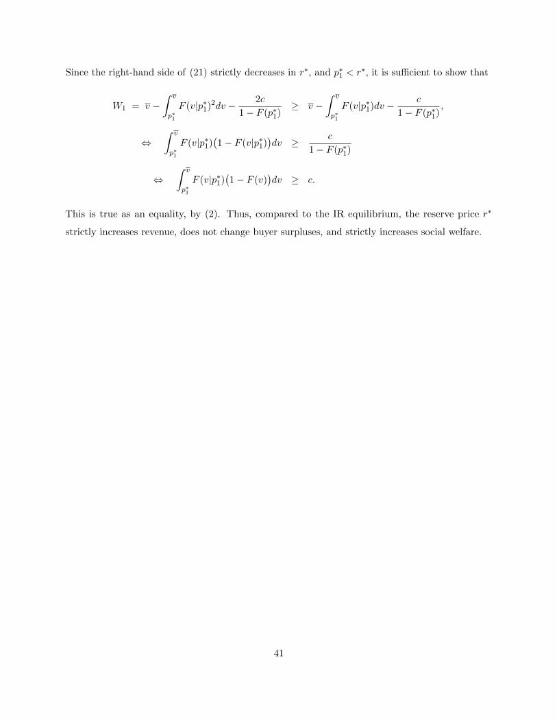
Since the right-hand side of (21) strictly decreases in r∗, and p∗1 < r∗, it is sufficient to show that

W1 = v −∫ v

p∗1

F (v|p∗1)2dv −2c

1− F (p∗1)≥ v −

∫ v

p∗1

F (v|p∗1)dv −c

1− F (p∗1),

⇔∫ v

p∗1

F (v|p∗1)(1− F (v|p∗1)

)dv ≥ c

1− F (p∗1)

⇔∫ v

p∗1

F (v|p∗1)(1− F (v)

)dv ≥ c.

This is true as an equality, by (2). Thus, compared to the IR equilibrium, the reserve price r∗

strictly increases revenue, does not change buyer surpluses, and strictly increases social welfare.

41