Entry deterrence and forward induction: An experiment *

Jordi Brandts, Antonio Cabrales, and Gary Charness

March 25, 2004

Abstract: The Dixit (1980) hypothesis that incumbents use investment in capacity to deterpotential entrants has found little empirical support. Bagwell and Ramey (1996) propose amodel where, in the unique game-theoretic prediction based on forward induction or iteratedelimination of weakly-dominated strategies, the incumbent does not have the strategic advantage.We conduct an experiment with games inspired by these models. In the Dixit-style game, theincumbent monopolizes the market most of the time even without the investment in capacity. Inour Bagwell-and-Ramey-style game, the incumbent also tends to keep the market, in contrast tothe predictions of a second-mover advantage. Nevertheless, we find strong evidence that forwardinduction affects the behavior of most participants. The results of our games suggest that playersperceive that the first mover has an advantage without having to pre-commit capacity. In ourBagwell-Ramey game, evolution and learning do not drive out this perception. We back theseclaims with data analysis, a theoretical framework for dynamics, and simulation results.

Keywords: entry, capacity investment, experiment, forward induction, equilibrium selection,first-mover advantage.

JEL Classification Numbers: C70, C91, D42, L11, L12

Authors’ Addresses

Jordi Brandts Antonio Cabrales Gary Charness

Institut d’Anàlisi Econòmica, CSICCampus UAB08193 BellaterraSpain

Department of Economics andBusinessUniversitat Pompeu FabraRamon Trias Fargas, 25-2708005 BarcelonaSpain

Department of Economics3031 North HallUniversity of CaliforniaSanta Barbara, CA 93106-9210USA

phone +34-93-5806612fax +34-93-5801452jordi.brandts@uab.es

phone +34-93-9514768fax +44-115-9514591antonio.cabrales@upf.edu

phone +1-805-8932412fax +1-805-8938830charness@econ.ucsb.edu

* Financial support by the Spanish Ministerio de Ciencia and Tecnología (SEC2002-01352) and the BarcelonaEconomic Program of CREA and excellent research assistance by David Rodríguez are gratefully acknowledged.The authors thank Armin Schmutzler for helpful comments.

1

1. INTRODUCTION

Theoretical industrial organization has argued, since Dixit (1980) and going back to Bain

(1956) and Modigliani (1958), that investment in capacity can be used to deter entry into

markets. This issue has received considerable attention in the industrial organization literature,

as one of the leading instances of the importance of commitment in sequential games.

References to and discussions of Dixit (1980) appear in virtually all the teaching manuals in the

area (see e.g. Tirole 1989, Basu 1993, Martin 1993 and Vives 1999). Despite this, there is little

empirical evidence that incumbent firms actually invest in capacity to deter entry (see, for

example, Smiley 1988 and Singh, Utton & Waterson 1998).1

Bagwell and Ramey (1996) provide a theoretical rationalization of this fact, based on a

new approach to the problem. The specific model they put forward has three principal

ingredients. First, it involves a different sequence of moves of the incumbent and the entrant

than the one proposed by Dixit. The other two ingredients are the existence of a partially-

recoverable capacity or entry cost and the use of forward induction to select among several

equilibria. In their model, there are typically monopoly equilibria in which either the incumbent

or the entrant captures the market, as well as market-sharing equilibria in which both firms

produce positive output levels. The main result is that forward induction rules out the equilibria

where the incumbent invests in capacity and, hence, does not retain the whole market. This

model yields a very suggestive explanation of observed behavior and invites further

investigation.

Given the highly stylized nature of the model, and the unobservability of some of the key

variables, a proper test of this model with field data is difficult. We therefore conduct

experiments to test the extent to which this explanation is satisfactory and, more generally, to

shed light on the strategic behavior of incumbents and entrants. Our work is an instance of the

kind of interplay between theory and data that experiments make possible. If our data turned out

to be consistent with the rationalization proposed by Bagwell and Ramey, this would

demonstrate the usefulness of forward induction in the context of an important issue in industrial

organization.

We use two stylized games inspired by, but somewhat different from, the game in

Bagwell and Ramey (1996), hereafter B-R and the game in Dixit (1980). In our B-R game, two

2

firms – an incumbent and a potential entrant – make decisions in three stages. First, the

incumbent has the opportunity to partially pre-commit to a given level of capacity, by incurring a

certain cost. Then the entrant has the same choice, having observed the incumbent’s choice. In

the third stage both firms simultaneously decide whether to compete (in prices) in the market, by

then paying (the rest of) the capacity cost. There are two pure-strategy equilibrium outcomes:

One of the two firms produces and obtains monopoly profit while the other stays out of the

market. Both of these situations are equilibrium outcomes resulting from backward induction.

However, only the outcome in which the incumbent leaves the market and the entrant

conquers it survives the application of iterated deletion of weakly-dominated strategies. In our

context, an entrant who pre-commits production must be signaling that she intends to become the

monopolist, as pre-committing and then not producing is a dominated strategy. The entrant

could have avoided pre-committing so as not to lose the pre-committed cost. In anticipation of

this, the incumbent does not pre-commit. Thus, in this game the possibility of partial pre-

commitment together with the logic of iterated weak dominance takes away the advantage that

the incumbent has in the standard entry-deterrence model.

There is one specific difference between the B-R game and ours that should be

highlighted here: In our game there are no market-sharing equilibria.2 The case with market-

sharing equilibria can be considered to be the empirically more reasonable one, since what the

field evidence suggests is that incumbents do not use capacity investment to keep other firms out

of the market and not so much that entrants can expel incumbents. It therefore would seem

natural to include market-sharing equilibria in the design. However, for evaluating the proposed

selection argument, an environment without the possibility for market-sharing is more

appropriate. The main reason is that market-sharing involves an element of fairness and this

feature could bias data in favor of this outcome. In addition, the exclusion of the possibility of

market-sharing eliminates potential coordination problems within the set of those equilibria that

survive the proposed selection argument. Our simple set-up allows for a cleaner comparison

between the two types of outcomes.

One might be tempted to question the suitability of this model to a field environment, since

there is nothing here that resembles past production, etc. Nevertheless, this model could represent

1 See also Geroski (1995) for a discussion of what is known empirically about entry.2 This also holds in the B-R game, under specific cost conditions.

3

a case where there is a new product. The incumbent produces a ‘nearby’ product and the entrant is

in a different line of business. An example can be seen in this quote from The Economist:3 “As

digital photography goes mainstream, the camera business is being transformed. One reason is that

digital cameras have as much in common with consumer-electronics devices as they do with film-

based cameras—so they are no longer the exclusive preserve of the traditional camera-makers.

The switch to digital provides an opportunity for new players to enter the market. The current

leaders in digital cameras, accounting for 75% of global sales are Canon, Sony, Olympus, Nikon,

and Kodak. But that line-up is volatile, with competition coming not just from consumer-

electronics giants, but also from PC-makers such as Hewlett-Packard, Dell and Gateway.”

We find that the full B-R prediction does not hold in our laboratory data. In fact, the

incumbent becomes the monopolist three times as frequently as the potential entrant. An

explanation of the tilt towards the incumbent may be found in a commonly-held belief by many

players that the first mover has a strategic advantage, and thus should become the monopolist in

the post-commitment game. In a less restrictive environment with ample market-sharing

possibilities this first-mover advantage might lead to incumbents capturing a larger part of

markets or capturing a given market with smaller expenditures on strategic investments. At the

same time, we find that there is only limited pre-commitment by either the incumbent or the

entrant. In our more standard entry game à la Dixit (1980), only the incumbent may pre-commit.

Here we find a considerably higher rate of incumbent entry deterrence through pre-commitment.

The quite moderate level of pre-commitment in our B-R design data is indeed suggestive,

as it is consistent with the field evidence. However, in what sense is it consistent with the more

frequent use of pre-commitment in the Dixit treatment? Perhaps the world is more like the B-R

environment, involving pre-commitment by both firms and partially recoverable costs; behavior

in the Dixit treatment may help us to understand behavior in the B-R environment. The pre-

conception of the first-mover advantage may be the starting point in both cases: In Dixit the pre-

commitment signal is a rather clear one and, hence, is used more frequently; it may be perceived

as the way to drive home the point of the incumbent’s first-mover advantage. In contrast, in B-R

the meaning of the combined signals may seem open to interpretation, and so pre-commitment is

used less frequently.

3 The Economist Technology Quarterly, March 13, 2004 (p. 14).

4

More generally in our games, when iterated weak dominance does not clash with a

perception of first-mover advantage, as in the case when only the first mover happens to pre-

commit or in the game when only one player can pre-commit, then the pre-committed player

becomes the monopolist with a very high likelihood. In these cases, the pre-commitment signal

is not indispensable but it helps, suggesting that most participants do have an understanding of

the basic iterated dominance force. In fact, we find compelling evidence that the choice of

whether or not to participate in the market is significantly affected by the pre-installation

decisions made.

The perceived first-mover advantage is only part of our explanation of the results. Even

if players were boundedly rational, one might expect that the opportunity to play the game

repeatedly could lead players to avoid dominated strategies, at least after enough time of play.

An initial perception of a first mover advantage would then vanish over time. It is, however,

well known that learning or evolution does not always lead to limiting outcomes that respect the

iterated deletion of weakly-dominated strategies.4 We provide some results that explain why the

initial pattern of play is not driven out. We show theoretically that our game has outcomes that

do not satisfy the iterated-deletion logic, but are asymptotically present under dynamics where

better-performing strategies grow faster than worse-performing ones. We also perform

simulations with a learning model (Camerer and Ho 1999) that tracks the behavior of our data.

2. IMPLEMENTATION

2.1. The B-R Game

In our B-R game there are two firms that can produce a homogeneous good with

constant, and equal, marginal cost. Production requires the building of a plant or some other

initial investment; the total cost of this initial investment is F. The game has three stages: In the

first and second stages, the incumbent and the entrant make sequential and observable capacity

pre-installation decisions. More precisely, the incumbent first chooses whether or not to

irrecoverably sink a fraction a < 1 of the fixed cost of production F . After observing the

incumbent’s choice the entrant then chooses between the same two options. In the third stage,

4 See, e.g., Fudenberg and Levine (1998), Samuelson (1997), Vega-Redondo (1996).

5

the two firms simultaneously make a decision on whether to compete in the market. This

decision involves either paying the remaining part of the full fixed cost, (1-a)F, or the whole

amount F. Thus, if one of the firms has not pre-committed, it can still pay for the total fixed cost

F in the third stage.

The third-stage competition is in prices. As a result, if both firms decide to actually pay

(the remainder of) the full capacity cost in the third stage, the resulting price will be equal to the

marginal cost. If only one of them chooses to pay the whole cost, then the outcome will be the

monopoly outcome. The only relevant actions in the third stage are, hence, whether or not to pay

(the remainder of) the whole fixed cost.

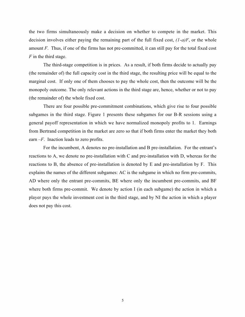
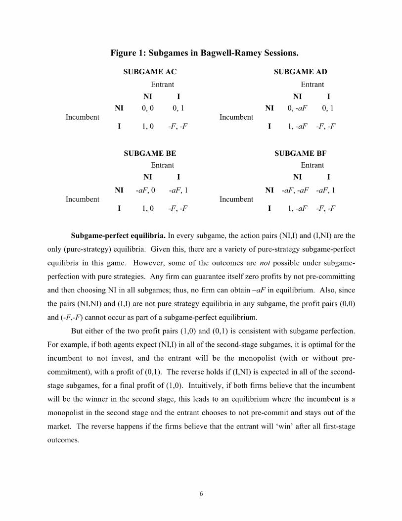
There are four possible pre-commitment combinations, which give rise to four possible

subgames in the third stage. Figure 1 presents these subgames for our B-R sessions using a

general payoff representation in which we have normalized monopoly profits to 1. Earnings

from Bertrand competition in the market are zero so that if both firms enter the market they both

earn –F. Inaction leads to zero profits.

For the incumbent, A denotes no pre-installation and B pre-installation. For the entrant’s

reactions to A, we denote no pre-installation with C and pre-installation with D, whereas for the

reactions to B, the absence of pre-installation is denoted by E and pre-installation by F. This

explains the names of the different subgames: AC is the subgame in which no firm pre-commits,

AD where only the entrant pre-commits, BE where only the incumbent pre-commits, and BF

where both firms pre-commit. We denote by action I (in each subgame) the action in which a

player pays the whole investment cost in the third stage, and by NI the action in which a player

does not pay this cost.

6

Figure 1: Subgames in Bagwell-Ramey Sessions.

SUBGAME AC SUBGAME AD

Entrant Entrant

NI I NI I

NI 0, 0 0, 1 NI 0, -aF 0, 1Incumbent Incumbent

I 1, 0 -F, -F I 1, -aF -F, -F

SUBGAME BE SUBGAME BF

Entrant Entrant

NI I NI I

NI -aF, 0 -aF, 1 NI -aF, -aF -aF, 1Incumbent Incumbent

I 1, 0 -F, -F I 1, -aF -F, -F

Subgame-perfect equilibria. In every subgame, the action pairs (NI,I) and (I,NI) are the

only (pure-strategy) equilibria. Given this, there are a variety of pure-strategy subgame-perfect

equilibria in this game. However, some of the outcomes are not possible under subgame-

perfection with pure strategies. Any firm can guarantee itself zero profits by not pre-committing

and then choosing NI in all subgames; thus, no firm can obtain –aF in equilibrium. Also, since

the pairs (NI,NI) and (I,I) are not pure strategy equilibria in any subgame, the profit pairs (0,0)

and (-F,-F) cannot occur as part of a subgame-perfect equilibrium.

But either of the two profit pairs (1,0) and (0,1) is consistent with subgame perfection.

For example, if both agents expect (NI,I) in all of the second-stage subgames, it is optimal for the

incumbent to not invest, and the entrant will be the monopolist (with or without pre-

commitment), with a profit of (0,1). The reverse holds if (I,NI) is expected in all of the second-

stage subgames, for a final profit of (1,0). Intuitively, if both firms believe that the incumbent

will be the winner in the second stage, this leads to an equilibrium where the incumbent is a

monopolist in the second stage and the entrant chooses to not pre-commit and stays out of the

market. The reverse happens if the firms believe that the entrant will ‘win’ after all first-stage

outcomes.

7

We have only discussed pure-strategy equilibria until now. The game has a variety of

mixed-strategy equilibria as well, and some of them are subgame-perfect. We will examine

mixed strategies in more detail in section 5.

2.2. Forward Induction

Matters change under certain refined equilibrium notions of subgame perfection, which

select a unique equilibrium from the set. Kohlberg and Mertens (1986) introduced the concept of

‘forward induction’ with the aim of describing some desirable properties of an equilibrium

concept. In general terms, forward induction says that the actions of players have strategic

significance, and should be interpreted in this light. It can be described (Battigalli 1996) in the

following way: “A player should always try to interpret her information about the behavior of

her opponents assuming that they are not implementing ‘irrational’ strategies.”5 In our case the

forward-induction rationality requirements imposed by Bagwell and Ramey seem relatively

mild. Players should avoid weakly-dominated strategies, and their opponents should be aware of

this, and take it into account when making their decisions.6

In our B-R game, forward induction gives the second mover an advantage. The argument

goes as follows: At the time of pre-commitment an entrant can guarantee himself a payoff of 0,

independently of what the incumbent has done, by not committing and then choosing NI. Thus,

any strategy under which a player pre-commits and then chooses NI is weakly dominated, as it

yields a lower payoff. Knowing that player 2 does not play dominated strategies, when player 1

observes a pre-commitment by player 2, he must conclude – according to the forward induction

logic - that player 2 intends to become the monopolist and will play I, and so player 1 will

respond optimally with NI.

As a consequence, player 2 will always (optimally) pre-commit, and then play I. In

contrast, pre-commitment does not have the same signaling value for the incumbent firm. An

incumbent that pre-committed could, mistakenly, have believed that the entrant was not going to

5 Forward induction (as with other refined equilibrium concepts, like strategic stability) has, nevertheless, interestingconnections with bounded rationality. For a rich discussion of the concept and formal definitions, see Hauk andHurkens (2002).6 An alternative definition by Van Damme (1989, p. 485) states that when: “player i chooses between an outside

option or to play a game G of which a unique (viable) equilibrium *e yields this player more than the outside option,

only the outcome in which i chooses G and *e is played is plausible.” It is easy to see that this (stronger) notionyields the same result in this game.

8

pre-commit (thus, expecting to become the monopolist). So, when faced with the unambiguous

subsequent pre-commitment choice of the entrant, the incumbent should yield and leave the

monopoly profits to the entrant. An incumbent who has not pre-committed has an even stronger

reason to yield in front of a pre-committed entrant. In anticipation of all this, the incumbent does

not pre-commit and leaves the market to the entrant.

Therefore, by forward induction, only the outcome (NI,I) is plausible. Taking this into

account, the first player will optimally respond by not pre-committing and then choosing NI in

all the subgames. So the set of strategies that survive the iterated deletion of weakly-dominated

strategies includes only the outcome (NI,I).

2.3. Iterated Deletion of Weakly-dominated Strategies

The corresponding reduced-normal form is shown in Table 1; it can be used to further

illustrate the selection rationale presented above. Here the incumbent is the row player and the

entrant the column player. The labels of the strategies are now those used in the experiment,

where the number “1” represents the choice of not completing the investment, NI, and the

number “2” means completing it, I. The reasoning we present holds for all positive values of a

and F. However, for ease of exposition, we now also use the same parameter values and payoffs

as in the experiment: We chose a = 1/2 and F = 1. We then transformed the payoffs by adding 1

to each payoff and then multiplying every payoff by 80. Thus, if both players choose I, each

receives 0. If only one player chooses I, he or she receives 160. Choosing NI gives a payoff of

80 without pre-installation; however, pre-installing and then choosing NI gives a payoff of 40.

9

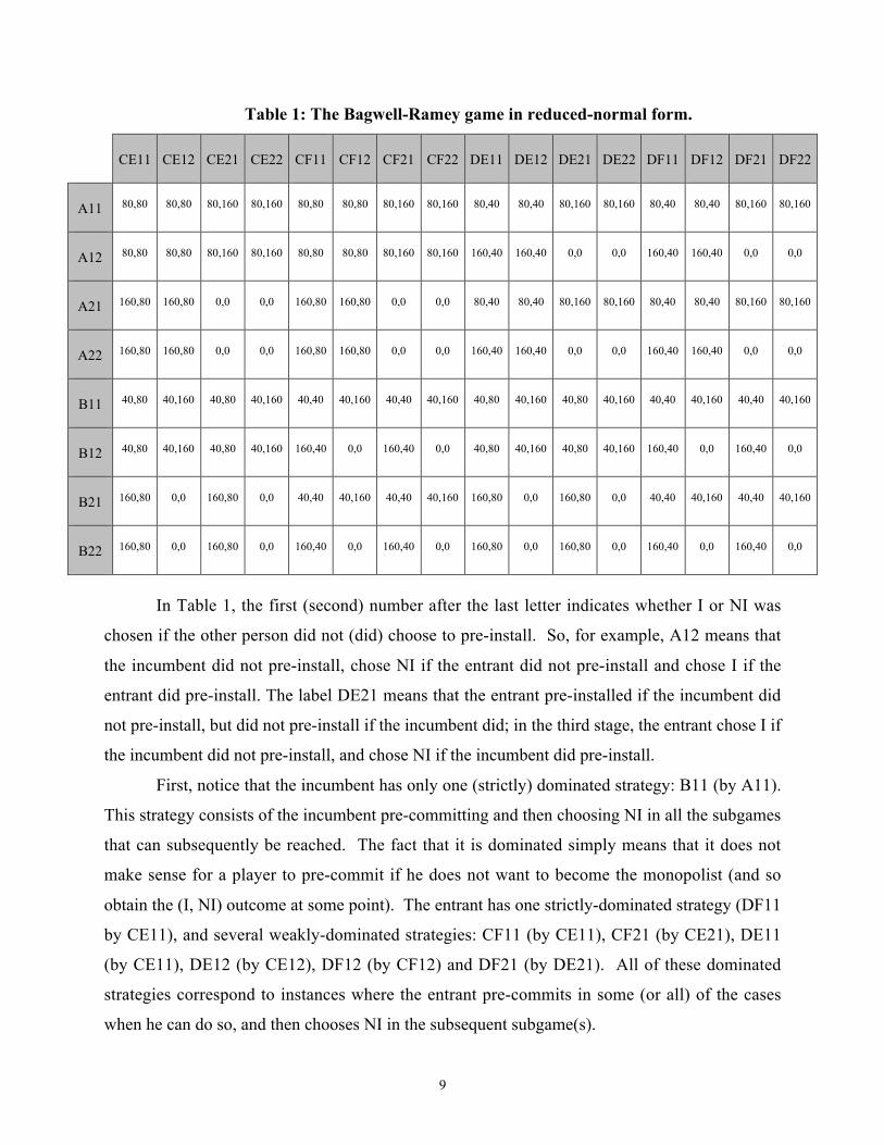
Table 1: The Bagwell-Ramey game in reduced-normal form.

CE11 CE12 CE21 CE22 CF11 CF12 CF21 CF22 DE11 DE12 DE21 DE22 DF11 DF12 DF21 DF22

A11 80,80 80,80 80,160 80,160 80,80 80,80 80,160 80,160 80,40 80,40 80,160 80,160 80,40 80,40 80,160 80,160

A12 80,80 80,80 80,160 80,160 80,80 80,80 80,160 80,160 160,40 160,40 0,0 0,0 160,40 160,40 0,0 0,0

A21 160,80 160,80 0,0 0,0 160,80 160,80 0,0 0,0 80,40 80,40 80,160 80,160 80,40 80,40 80,160 80,160

A22 160,80 160,80 0,0 0,0 160,80 160,80 0,0 0,0 160,40 160,40 0,0 0,0 160,40 160,40 0,0 0,0

B11 40,80 40,160 40,80 40,160 40,40 40,160 40,40 40,160 40,80 40,160 40,80 40,160 40,40 40,160 40,40 40,160

B12 40,80 40,160 40,80 40,160 160,40 0,0 160,40 0,0 40,80 40,160 40,80 40,160 160,40 0,0 160,40 0,0

B21 160,80 0,0 160,80 0,0 40,40 40,160 40,40 40,160 160,80 0,0 160,80 0,0 40,40 40,160 40,40 40,160

B22 160,80 0,0 160,80 0,0 160,40 0,0 160,40 0,0 160,80 0,0 160,80 0,0 160,40 0,0 160,40 0,0

In Table 1, the first (second) number after the last letter indicates whether I or NI was

chosen if the other person did not (did) choose to pre-install. So, for example, A12 means that

the incumbent did not pre-install, chose NI if the entrant did not pre-install and chose I if the

entrant did pre-install. The label DE21 means that the entrant pre-installed if the incumbent did

not pre-install, but did not pre-install if the incumbent did; in the third stage, the entrant chose I if

the incumbent did not pre-install, and chose NI if the incumbent did pre-install.

First, notice that the incumbent has only one (strictly) dominated strategy: B11 (by A11).

This strategy consists of the incumbent pre-committing and then choosing NI in all the subgames

that can subsequently be reached. The fact that it is dominated simply means that it does not

make sense for a player to pre-commit if he does not want to become the monopolist (and so

obtain the (I, NI) outcome at some point). The entrant has one strictly-dominated strategy (DF11

by CE11), and several weakly-dominated strategies: CF11 (by CE11), CF21 (by CE21), DE11

(by CE11), DE12 (by CE12), DF12 (by CF12) and DF21 (by DE21). All of these dominated

strategies correspond to instances where the entrant pre-commits in some (or all) of the cases

when he can do so, and then chooses NI in the subsequent subgame(s).

10

Once the weakly-dominated strategies of the entrant have been eliminated, the incumbent

has some weakly-dominated strategies: A12 (by A11), A22 (by A21), B12 (by A11) and B22 (by

B21). All of these strategies correspond to instances where the incumbent chooses I in a

subgame where the entrant has chosen to pre-commit. That can only be optimal if the entrant

chose NI in that subgame. However, such choices by the entrant are dominated, and have

already been eliminated.

The strategy DF22 for the entrant is now weakly dominant among the remaining

strategies. This strategy corresponds to the entrant always pre-committing and then choosing I in

all subgames. This is dominant because the (serially) undominated choice of the incumbent is to

play NI any time he ‘observes’ a pre-commitment by the entrant. Finally, since DF22 is

dominant, incumbent strategy B21 is sub-optimal, and the only strategies that remain for the

incumbent are A11 and A21. So the prediction is that the incumbent will not pre-commit, but

that the entrant will pre-commit and then become the monopolist.7

It is worth noticing that even without performing this last iteration (that is, with just two

rounds of deletion of dominated strategies), the entrant can guarantee his favorite outcome (NI,

I), as all the equilibria in the game that remains after two rounds of deletion produce that

outcome. In some of those equilibria the entrant does not even have to pre-commit. A less

stringent and perhaps more robust prediction would, therefore, be that the entrant becomes the

monopolist with or without pre-installation.

One may think that most people will not be able to follow the kind of logic that forward

induction involves. However, a number of experimental studies report results that are favorable

to forward induction. Cooper, DeJong, Forsythe & Ross (1992) analyze experiments involving a

choice between an outside option for one of the players and a 2x2 coordination game, with two

Pareto-ranked equilibria. They analyze the case where forward induction and a simple

dominance argument lead to the same prediction, and their results are consistent with this kind of

forward-induction concept. Cooper, DeJong, Forsythe & Ross (1993) present results from an

experimental game, where there is an outside option for one of the players and a symmetric

Battle-of-the-Sexes game is played if this outside option is foregone. When forward induction

7 In general, the order of deletion of weakly dominated strategies might affect the final outcome of a given game.Not so in ours. The reason is that the strategies that are dominated (thus, eliminated) in (our) second round do notaffect the relationship between those that are dominated and dominant in (our) first round. For example, after just

11

coincides with simple dominance the results are again consistent with these notions. However,

in a second treatment, an outside option that does not dominate one of the other choices in the

Battle-of-the-Sexes affects play in the same manner as an outside option that does dominate.

Van Huyck, Battalio & Beil (1993) consider an experimental setting in which players

participate in an auction for the right to play a coordination game. Their results exhibit two key

features: The price in the auction is high enough for a forward induction argument (different

from dominance here) to select the Pareto-efficient equilibrium, and subjects’ play in the

coordination game actually selects this equilibrium. Broseta, Fatás and Neugenauer (2003)

report evidence favorable to forward induction in an experiment in which subjects first bid in an

auction and subsequently play a game with several equilibria. The results presented in Brandts

and Holt (1995) support forward induction in a very simple game where it is equivalent to the

elimination of dominated strategies, but not in two more demanding environments.

There is also evidence that suggests that forward induction is not an important behavioral

force. Schotter, Weigelt & Wilson (1994) study an experimental game for which the application

of iterated dominance selects one outcome and obtain results that are not consistent with the

predictions of the iterated dominance argument. Balkenborg (1998) reports results from a game

in which backward induction yields an outcome different from that resulting from forward

induction arguments; less than 20% of all cases result in the forward-induction outcome.

Overall, it seems that the jury is still out on the matter. We are still far from having

delineated the circumstances under which forward induction is and is not consistent with

people’s behavior in the laboratory. Only a large accumulation of studies will make it possible

to obtain a global view on the empirical usefulness of forward induction. Given this context, we

feel it is useful to study the predictive validity of forward induction in an environment that is of

interest in relation to an important issue in industrial organization.

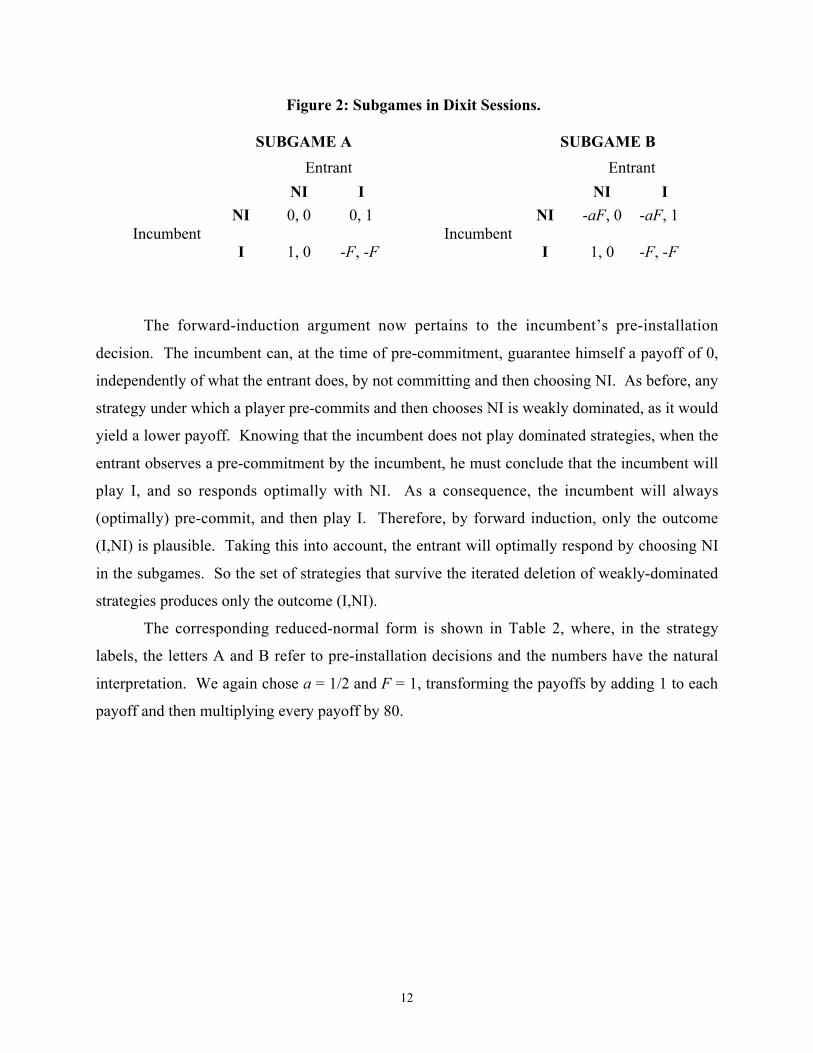
2.4. The Dixit Game

In our Dixit games, only the incumbent could pre-install, leading to only the two

subgames shown in Figure 2:

eliminating DE11, DE12, DF11 and DF12, we can eliminate A12 and A22. Even after this deletion CF11, CF21and DF21 are still weakly dominated by the same strategies we used.

12

Figure 2: Subgames in Dixit Sessions.

SUBGAME A SUBGAME B

Entrant Entrant

NI I NI I

NI 0, 0 0, 1 NI -aF, 0 -aF, 1Incumbent Incumbent

I 1, 0 -F, -F I 1, 0 -F, -F

The forward-induction argument now pertains to the incumbent’s pre-installation

decision. The incumbent can, at the time of pre-commitment, guarantee himself a payoff of 0,

independently of what the entrant does, by not committing and then choosing NI. As before, any

strategy under which a player pre-commits and then chooses NI is weakly dominated, as it would

yield a lower payoff. Knowing that the incumbent does not play dominated strategies, when the

entrant observes a pre-commitment by the incumbent, he must conclude that the incumbent will

play I, and so responds optimally with NI. As a consequence, the incumbent will always

(optimally) pre-commit, and then play I. Therefore, by forward induction, only the outcome

(I,NI) is plausible. Taking this into account, the entrant will optimally respond by choosing NI

in the subgames. So the set of strategies that survive the iterated deletion of weakly-dominated

strategies produces only the outcome (I,NI).

The corresponding reduced-normal form is shown in Table 2, where, in the strategy

labels, the letters A and B refer to pre-installation decisions and the numbers have the natural

interpretation. We again chose a = 1/2 and F = 1, transforming the payoffs by adding 1 to each

payoff and then multiplying every payoff by 80.

13

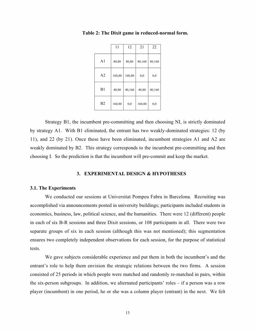
Table 2: The Dixit game in reduced-normal form.

11 12 21 22

A1 80,80 80,80 80,160 80,160

A2 160,80 160,80 0,0 0,0

B1 40,80 40,160 40,80 40,160

B2 160,80 0,0 160,80 0,0

Strategy B1, the incumbent pre-committing and then choosing NI, is strictly dominated

by strategy A1. With B1 eliminated, the entrant has two weakly-dominated strategies: 12 (by

11), and 22 (by 21). Once these have been eliminated, incumbent strategies A1 and A2 are

weakly dominated by B2. This strategy corresponds to the incumbent pre-committing and then

choosing I. So the prediction is that the incumbent will pre-commit and keep the market.

3. EXPERIMENTAL DESIGN & HYPOTHESES

3.1. The Experiments

We conducted our sessions at Universitat Pompeu Fabra in Barcelona. Recruiting was

accomplished via announcements posted in university buildings; participants included students in

economics, business, law, political science, and the humanities. There were 12 (different) people

in each of six B-R sessions and three Dixit sessions, or 108 participants in all. There were two

separate groups of six in each session (although this was not mentioned); this segmentation

ensures two completely independent observations for each session, for the purpose of statistical

tests.

We gave subjects considerable experience and put them in both the incumbent’s and the

entrant’s role to help them envision the strategic relations between the two firms. A session

consisted of 25 periods in which people were matched and randomly re-matched in pairs, within

the six-person subgroups. In addition, we alternated participants’ roles – if a person was a row

player (incumbent) in one period, he or she was a column player (entrant) in the next. We felt

14

that this alternation scheme offered the best chance for people to understand the subtleties

involved. The full instructions can be found in Appendix A.

People received their earnings over the 25 periods played in a session, with nominal

payoffs re-normalized for experimental purposes. Average payoffs for the two-hour sessions

were around 2500 pesetas, including a show-up fee of 500 pesetas (at the time, $1 exchanged for

approximately 180 pesetas).

Our games were played using the strategy-elicitation method. This means that the

incumbent had to choose whether to pre-install or not and also whether to complete the

investment or not for each of the entrant’s possible pre-installation decisions in the second stage.

Similarly, the entrant had to make a pre-installation decision for the incumbent’s two possible

pre-installation decisions, as well as a complete investment decision for the two possible

resulting pre-installation decisions of the two players.

In the B-R sessions play proceeded as follows: Each incumbent stated whether he wished

to pre-commit, and also stated a choice (I or NI) for each of the two cases regarding possible pre-

commitment by the entrant. Using the labels of the game above, the incumbent had to choose

between A and B, and to indicate his choice in the two possible subgames that could result from

the choice between A and B. Each entrant made choices without being informed of the paired

incumbent’s choices and stated whether she wished to pre-commit if the incumbent had pre-

committed and also whether she wished to pre-commit if the incumbent had not pre-committed.8

Given her own pre-commitment choices, she also stated a choice (I or NI) for each of the two

cases regarding possible pre-commitment by the incumbent. She had to indicate her choice both

for A and for B, as well as her choices for the two possible resulting subgames. After the data

for the period was collected and matched up, each participant was informed of his or her payoff

outcome for that period.

In the Dixit sessions, the incumbent stated his choice concerning pre-commitment, as

well as his choice (I or NI) in the resulting subgame. The entrant stated a choice (I or NI) if the

incumbent had pre-committed and also if the incumbent had not pre-committed.

8 We shall henceforth presume that the incumbent is male and the entrant is female, despite the fact that one’sgender must therefore change each period.

15

3.2. Hypotheses

To help organize the discussion of our data, we state null and alternative hypotheses

concerning influences on outcomes and behavior in our experimental games. We test these

hypotheses in section 4.2 of the paper. In our context the most fundamental question is,

arguably, which of the two players captures the market. The answer represents the bottom line

with respect to the theoretical prediction. Our first set of hypotheses pertains to this question.

The negation of the B-R and Dixit predictions pertaining to firms’ strategic advantage

gives rise to the following two null hypotheses:

Hypothesis 1: Neither the incumbent nor the entrant will monopolize the market morefrequently than the other in the B-R game.

Hypothesis 2: Neither the incumbent nor the entrant will monopolize the market morefrequently than the other in the Dixit game.

On the other hand, the theoretical predictions are clear for our experimental games: There

is a first-mover advantage in the Dixit game and a second-mover advantage in the B-R game.

These predictions lead to two alternative hypotheses:

Hypothesis 1a: The incumbent will monopolize the market more frequently than theentrant in the B-R game.

Hypothesis 2a: The entrant will monopolize the market more frequently than theincumbent in the Dixit game.

Regardless of the nature of the market outcomes, if forward induction or the iterated

elimination of weakly-dominated strategies have no influence in our experimental games, pre-

installation choices should not affect firms’ subsequent decisions to participate in the market:

Hypothesis 3: The likelihood that a firm will choose to participate in the market is notaffected by whether the firm or its competitor has chosen to pre-install capacity.

As we expect forward induction or iterated deletion to influence players’ choices in both

of our experimental games, our alternative hypothesis is:

16

Hypothesis 3a: A firm is more likely to choose to participate in the market if it haschosen to pre-install capacity and is less likely to participate in the market if the otherfirm has chosen to pre-install capacity.

4. EXPERIMENTAL RESULTS

4.1. Realized Outcomes

We first present an overview of the main features of our results; in section 4.2 we present

results corresponding to our hypotheses above. In section 5 below we discuss subjects’ observed

strategy choices and connect this to our simulation and theoretical analysis. Our first focus is the

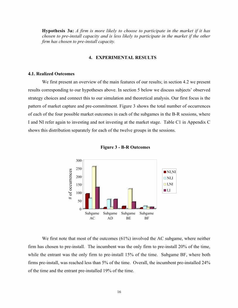
pattern of market capture and pre-commitment. Figure 3 shows the total number of occurrences

of each of the four possible market outcomes in each of the subgames in the B-R sessions, where

I and NI refer again to investing and not investing at the market stage. Table C1 in Appendix C

shows this distribution separately for each of the twelve groups in the sessions.

0

50

100

150

200

250

300

# of

occ

urre

nces

SubgameAC

SubgameAD

SubgameBE

SubgameBF

Figure 3 - B-R Outcomes

NI,NI

NI,I

I,NI

I,I

We first note that most of the outcomes (61%) involved the AC subgame, where neither

firm has chosen to pre-install. The incumbent was the only firm to pre-install 20% of the time,

while the entrant was the only firm to pre-install 15% of the time. Subgame BF, where both

firms pre-install, was reached less than 5% of the time. Overall, the incumbent pre-installed 24%

of the time and the entrant pre-installed 19% of the time.

17

With respect to market capture, in the B-R games, the result is that the entrant becomes

the monopolist only 15% of the time; by comparison, the incumbent becomes the monopolist in

45% of the cases. Coordination failure is substantial with no one in the market 13% of the time

and both players in the market 27% of the time. Note, however, that together this 40% is still

below the rate of coordination on the incumbent becoming the monopolist.

The natural next question is whether the incumbent’s preponderance is accomplished

through his pre-commitment. When there is no pre-installation, the incumbent becomes the

monopolist 48% of the time (the corresponding figure for the entrant is 12%). When only the

incumbent pre-installs, he becomes the monopolist 69% of the time (the corresponding figure for

the entrant is 44%), so that pre-commitment does help the incumbent. Taken together these facts

allow us to say that the incumbent wins the market frequently and rather effortlessly, more so

than the entrant, in contrast to what theory suggests.

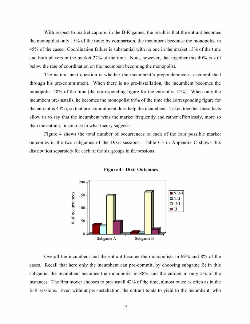
Figure 4 shows the total number of occurrences of each of the four possible market

outcomes in the two subgames of the Dixit sessions. Table C3 in Appendix C shows this

distribution separately for each of the six groups in the sessions.

0

50

100

150

200

# of

occ

urre

nces

Subgame A Subgame B

Figure 4 - Dixit Outcomes

NI,NINI,II,NII,I

Overall the incumbent and the entrant become the monopolists in 69% and 8% of the

cases. Recall that here only the incumbent can pre-commit, by choosing subgame B; in this

subgame, the incumbent becomes the monopolist in 88% and the entrant in only 2% of the

instances. The first mover chooses to pre-install 42% of the time, almost twice as often as in the

B-R sessions. Even without pre-installation, the entrant tends to yield to the incumbent, who

18

becomes the monopolist 56% of the time, compared to 12% for the entrant. The orderings of

these percentages is qualitatively similar to those in the B-R sessions (with no entrant pre-

installation). The relevant rates are here 69% and 0% when the incumbent pre-installs (BE in the

B-R sessions) and 48% and 12% when she doesn’t (AC). The pattern of conditional investment

decisions is similar to that in the B-R sessions: when the incumbent does not pre-install,

incumbent and entrant complete the investment in 75% and 30% of the cases, whereas with pre-

installation these figures are 95% and 5%.

We now focus on different comparisons involving observed frequencies in the different

subgames, which we use to more clearly highlight the degree of support for the general notion of

pre-commitment as a tool for market control. In the B-R games, we start by observing that the

incumbent’s pre-installation has only a minor impact on the entrant’s pre-installation rate: The

entrant chooses to pre-install 17% of the time when the incumbent pre-installs, compared to 21%

of the time when the incumbent does not pre-install.

At this point one might be tempted to jump to the conclusion that the strategic principles

put forward in game-theoretic analysis have no effect, even in its most basic form. Nevertheless,

pre-commitment by at least one firm occurs frequently enough in our data to warrant an

examination of how firms’ pre-commitment patterns and their relation to final investment (entry)

decisions affect subsequent choices. We next compare decisions within and across subgames,

and find that players’ decisions on whether to compete in the market are quite sensitive to pre-

installation choices of themselves and their counterparts.

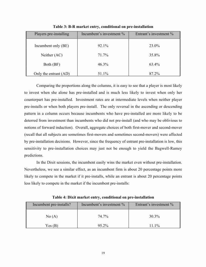
Table 3 shows the proportion of eventual entry (choices of I strategies) into the market

for each player in the B-R sessions, contingent on pre-installation decisions. Focusing first on

comparisons within rows in the table, we observe the following pattern: When only one of the

players pre-installs that player completes the investment more frequently and, hence, can be

thought of having an advantage in capturing the market. When neither pre-installs the incumbent

completes the investment more frequently than the entrant; when both pre-install, the investment

rate is somewhat higher for the entrant.

19

Table 3: B-R market entry, conditional on pre-installation

Players pre-installing Incumbent’s investment % Entrant’s investment %

Incumbent only (BE) 92.1% 23.0%

Neither (AC) 71.7% 35.8%

Both (BF) 46.3% 63.4%

Only the entrant (AD) 51.1% 87.2%

Comparing the proportions along the columns, it is easy to see that a player is most likely

to invest when she alone has pre-installed and is much less likely to invest when only her

counterpart has pre-installed. Investment rates are at intermediate levels when neither player

pre-installs or when both players pre-install. The only reversal in the ascending or descending

pattern in a column occurs because incumbents who have pre-installed are more likely to be

deterred from investment than incumbents who did not pre-install (and who may be oblivious to

notions of forward induction). Overall, aggregate choices of both first-mover and second-mover

(recall that all subjects are sometimes first-movers and sometimes second-movers) were affected

by pre-installation decisions. However, since the frequency of entrant pre-installation is low, this

sensitivity to pre-installation choices may just not be enough to yield the Bagwell-Ramey

predictions.

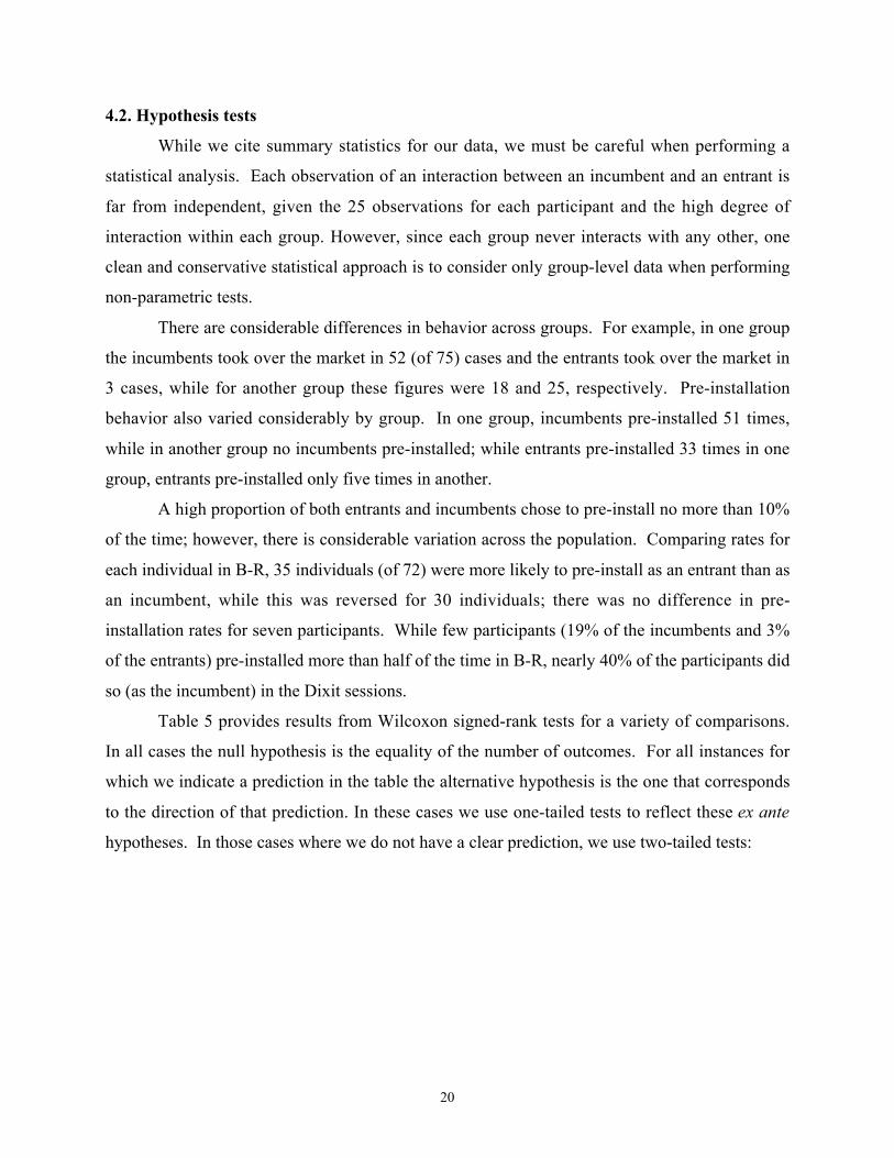
In the Dixit sessions, the incumbent easily wins the market even without pre-installation.

Nevertheless, we see a similar effect, as an incumbent firm is about 20 percentage points more

likely to compete in the market if it pre-installs, while an entrant is about 20 percentage points

less likely to compete in the market if the incumbent pre-installs:

Table 4: Dixit market entry, conditional on pre-installation

Incumbent pre-installs? Incumbent’s investment % Entrant’s investment %

No (A) 74.7% 30.3%

Yes (B) 95.2% 11.1%

20

4.2. Hypothesis tests

While we cite summary statistics for our data, we must be careful when performing a

statistical analysis. Each observation of an interaction between an incumbent and an entrant is

far from independent, given the 25 observations for each participant and the high degree of

interaction within each group. However, since each group never interacts with any other, one

clean and conservative statistical approach is to consider only group-level data when performing

non-parametric tests.

There are considerable differences in behavior across groups. For example, in one group

the incumbents took over the market in 52 (of 75) cases and the entrants took over the market in

3 cases, while for another group these figures were 18 and 25, respectively. Pre-installation

behavior also varied considerably by group. In one group, incumbents pre-installed 51 times,

while in another group no incumbents pre-installed; while entrants pre-installed 33 times in one

group, entrants pre-installed only five times in another.

A high proportion of both entrants and incumbents chose to pre-install no more than 10%

of the time; however, there is considerable variation across the population. Comparing rates for

each individual in B-R, 35 individuals (of 72) were more likely to pre-install as an entrant than as

an incumbent, while this was reversed for 30 individuals; there was no difference in pre-

installation rates for seven participants. While few participants (19% of the incumbents and 3%

of the entrants) pre-installed more than half of the time in B-R, nearly 40% of the participants did

so (as the incumbent) in the Dixit sessions.

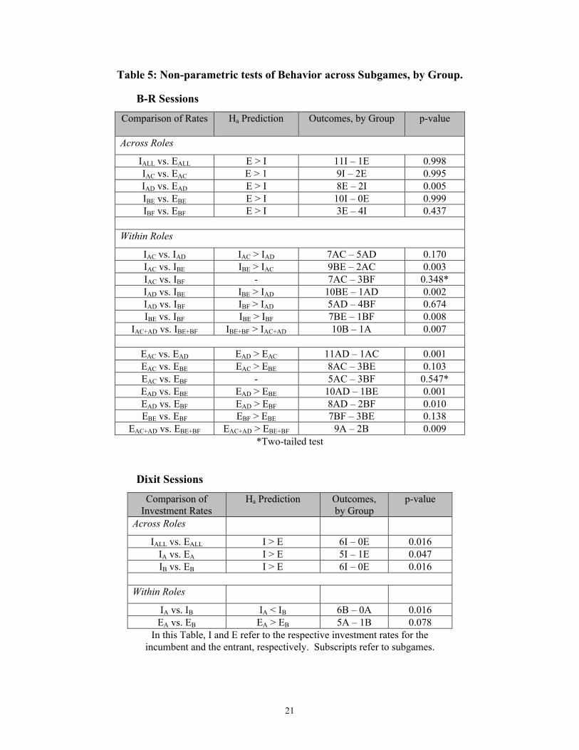
Table 5 provides results from Wilcoxon signed-rank tests for a variety of comparisons.

In all cases the null hypothesis is the equality of the number of outcomes. For all instances for

which we indicate a prediction in the table the alternative hypothesis is the one that corresponds

to the direction of that prediction. In these cases we use one-tailed tests to reflect these ex ante

hypotheses. In those cases where we do not have a clear prediction, we use two-tailed tests:

21

Table 5: Non-parametric tests of Behavior across Subgames, by Group.

B-R Sessions

Comparison of Rates Ha Prediction Outcomes, by Group p-value

Across Roles

IALL vs. EALL E > I 11I – 1E 0.998IAC vs. EAC E > 1 9I – 2E 0.995IAD vs. EAD E > I 8E – 2I 0.005IBE vs. EBE E > I 10I – 0E 0.999IBF vs. EBF E > I 3E – 4I 0.437

Within Roles

IAC vs. IAD IAC > IAD 7AC – 5AD 0.170IAC vs. IBE IBE > IAC 9BE – 2AC 0.003IAC vs. IBF - 7AC – 3BF 0.348*IAD vs. IBE IBE > IAD 10BE – 1AD 0.002IAD vs. IBF IBF > IAD 5AD – 4BF 0.674IBE vs. IBF IBE > IBF 7BE – 1BF 0.008

IAC+AD vs. IBE+BF IBE+BF > IAC+AD 10B – 1A 0.007

EAC vs. EAD EAD > EAC 11AD – 1AC 0.001EAC vs. EBE EAC > EBE 8AC – 3BE 0.103EAC vs. EBF - 5AC – 3BF 0.547*EAD vs. EBE EAD > EBE 10AD – 1BE 0.001EAD vs. EBF EAD > EBF 8AD – 2BF 0.010EBE vs. EBF EBF > EBE 7BF – 3BE 0.138

EAC+AD vs. EBE+BF EAC+AD > EBE+BF 9A – 2B 0.009*Two-tailed test

Dixit Sessions

Comparison ofInvestment Rates

Ha Prediction Outcomes,by Group

p-value

Across Roles

IALL vs. EALL I > E 6I – 0E 0.016IA vs. EA I > E 5I – 1E 0.047IB vs. EB I > E 6I – 0E 0.016

Within Roles

IA vs. IB IA < IB 6B – 0A 0.016EA vs. EB EA > EB 5A – 1B 0.078

In this Table, I and E refer to the respective investment rates for theincumbent and the entrant, respectively. Subscripts refer to subgames.

22

In the B-R game, while the incumbent is significantly more likely to control the market

when the entrant does not pre-install (subgames AC and BE), the entrant is significantly more

likely to control the market when she pre-installs and the incumbent does not (subgame AD);

there does not appear to be a consensus when both pre-install. In the Dixit game, the incumbent

controls the market in all cases.

Let us consider Hypothesis 1: Is there a pattern concerning which firm captures the

market? The comparison in the very first row, IALL vs. EALL, pertains to which of the two players

becomes the monopolist. The 11I-1E comparison means that the incumbent became the

monopolist more frequently (overall) than did the entrant in 11 of the 12 groups.9 The null

hypothesis is clearly rejected, as the Wilcoxon signed-rank test tells us that a disparity this

extreme will only occur 0.4% of the time.10 However, this result provides very little support for

Hypothesis1a, as there is a significant tendency for the incumbent to control the market, rather

than the entrant.

The first row of the Dixit-sessions sub-table, IALL vs. EALL, provides a test of Hypothesis

2 and Hypothesis 2a. The 6I-0E comparison means that the incumbent became the monopolist

more frequently (overall) than did the entrant in all six of the groups. The Wilcoxon signed-rank

test easily rejects the null hypothesis, here in favor of Hypothesis 2a at p < 0.002. Thus, here

there is also a strong tendency for the incumbent to capture the market, in this case as predicted

by forward induction.

The within-role comparisons pertain to Hypothesis 3 and Hypothesis 3a. The tests

confirm that investment rates are typically affected, and in the direction expected, by pre-

installation decisions. The B-R group tests also confirm that the incumbent is significantly more

likely to invest after she has pre-installed than after she has not pre-installed (p = 0.007), and that

the entrant is significantly less likely to invest after the incumbent pre-installs (p = 0.009). The

differences are particularly strong for own pre-installation decisions, and no more than one party

9 For all other across-role comparisons we compare, for each group, the number of times that the incumbent investedvs. the number of times the entrant invested. So, for example, the 9I-2E in the second row under Across Rolesmeans that the incumbent invested more frequently than did the entrant in 9 of 11 groups. For within-rolecomparisons, we consider the incumbent and entrant investment rates for each group. So, for example, the 9BE-2AC in the second row under Within Roles means that the incumbents invested more frequently in subgame BE thanin subgame AC for nine of 11 groups. While we have data for 12 groups, there are often ties and/or cases whereinvestment rates in a category cannot be calculated (a zero divisor), so the number of comparisons is frequently lessthan 12.10 This test considers not only the direction of differences, but also considers the magnitude of the difference (seeSiegel and Castellan 1988).

23

pre-installs; we see that IBE > IAC, IBE > IAD, EAC < EAD, and EBE < EAD, all at easily significant

levels. Similarly, the incumbent in the Dixit sessions invests more often in all sessions when he

has pre-installed, while the entrant invests less in five of the six sessions when the incumbent

pre-installs. All of these data reject Hypothesis 3 in favor of Hypothesis 3a.

Nevertheless, the effects are not as strong for within-role comparisons that reflect

whether or not the other party has pre-installed. Both the EBE vs. EAC and the IAC vs. IAD

comparisons show that there is some (not-quite-significant) tendency to respect the other firm’s

pre-installation choice. The only significant within-role comparisons involving the BF subgame

are the cases where the role player has pre-installed (IBE vs. IBF and EAD vs. EBF), suggesting that

a player who understands the logic of pre-installation is more likely to be sensitive to the pre-

installation decisions of others.

5. STRATEGIES, DYNAMICS & SIMULATIONS

5.1. Strategy ChoicesOur results may look somewhat puzzling given the theoretical discussion in section 2.

After all, the solution via deletion of dominated strategies looks sensible, given that only a few

rounds of elimination are necessary. One obvious explanation is that the rationality of

experimental subjects is lower than what is necessary for achieving the theoretical outcome. But,

one may wonder just how irrational these agents are. Up to now we have provided a rather

synthesized view of the results. Since we elicit full strategies for each player, to obtain a more

in-depth view of subjects’ behavior we can also examine the frequency of play for each strategy,

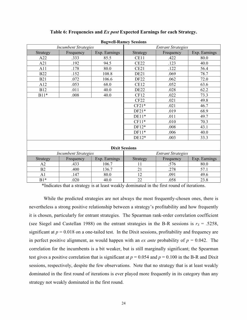
as well as its expected earnings. Table 6 displays this information for the B-R and Dixit

sessions, where strategies have been ordered by the frequency of their choice. The number of

times each strategy was chosen in each B-R and Dixit group is shown, respectively, in Tables C2

and C4 of Appendix C.

24

Table 6: Frequencies and Ex post Expected Earnings for each Strategy.

Bagwell-Ramey SessionsIncumbent Strategies Entrant Strategies

Strategy Frequency Exp. Earnings Strategy Frequency Exp. EarningsA22 .333 85.5 CE11 .422 80.0A21 .192 94.5 CE22 .123 40.0A11 .178 80.0 CE21 .122 56.4B22 .152 108.8 DE21 .069 78.7B21 .072 106.6 DF22 .062 72.0A12 .053 68.0 CE12 .052 63.6B12 .011 40.0 DE22 .028 62.2B11* .008 40.0 CF12 .022 73.3

CF22 .021 49.8CF21* .021 46.7DF21* .019 68.9DE11* .011 49.7CF11* .010 70.3DF12* .008 43.1DF11* .006 40.0DE12* .003 33.3

Dixit SessionsIncumbent Strategies Entrant Strategies

Strategy Frequency Exp. Earnings Strategy Frequency Exp. EarningsA2 .433 106.7 11 .576 80.0B2 .400 136.7 21 .278 57.1A1 .147 80.0 12 .091 49.6B1* .020 40.0 22 .058 23.8*Indicates that a strategy is at least weakly dominated in the first round of iterations.

While the predicted strategies are not always the most frequently-chosen ones, there is

nevertheless a strong positive relationship between a strategy’s profitability and how frequently

it is chosen, particularly for entrant strategies. The Spearman rank-order correlation coefficient

(see Siegel and Castellan 1988) on the entrant strategies in the B-R sessions is rS = .5258,

significant at p = 0.018 on a one-tailed test. In the Dixit sessions, profitability and frequency are

in perfect positive alignment, as would happen with an ex ante probability of p = 0.042. The

correlation for the incumbents is a bit weaker, but is still marginally significant; the Spearman

test gives a positive correlation that is significant at p = 0.054 and p = 0.100 in the B-R and Dixit

sessions, respectively, despite the few observations. Note that no strategy that is at least weakly

dominated in the first round of iterations is ever played more frequently in its category than any

strategy not weakly dominated in the first round.

25

B-R sessions. Recall that the two incumbent strategies that should be played according

to forward induction in the B-R equilibrium are A11 and A21. A11, the completely safe strategy,

is chosen almost 18% of the time. A21 is like A11 except that it chooses I if player 2 does not

pre-install. It does better than the more aggressive A22 strategy, as the expected payoff from

playing I in AD is only 21.6, compared to 80 for NI. In fact, many people follow these

incentives – A21 is played 19% of the time, and does best of all the no-pre-installation strategies.

So the incumbent strategies consistent with B-R equilibrium are played 37% of the time.

The most commonly-used incumbent strategy (33.3%, by far the highest) is A22 (do not

pre-install and always invest later. A22 has an expected ex post payoff of 85.5, better than the

safe payoff of 80 that is available by not pre-installing and never investing (A11). Choosing A22

is consistent with the simple view that everyone knows that the first mover has the advantage.

Nevertheless, the first mover could increase own payoffs by choosing A21, which only differs

from A22 in that the incumbent chooses not to complete the investment if he observes pre-

installation by the second player. He would earn even more by just pre-installing and playing

B21 or, even better, B22 (so certainly play I if the second player does not pre-install). Pre-

installing really clears the way for the incumbent’s market dominance here.

The most profitable incumbent strategy, B22, is chosen 15.2% of the time; in fact, the

frequency with which it is chosen is gradually growing (11%, 14%, 17%, and 19% in periods 1-

5, 6-10, 11-15, 16-20, and 21-25, respectively). B21 is like B22, except that it chooses NI if the

second player pre-installs, and offers a very good expected payoff. It is chosen 7% of the time,

with a frequency roughly ‘stable’ over time). Finally, A12, B11, and B12 are played with such

low frequencies that one may view them as errors or experiments.

The most common entrant strategy, used in 42.2% of the cases, is CE11, which consists

of never pre-installing, then always playing NI and, hence, staying out of the market. It was

chosen more than three times as frequently as any other strategy, and in fact this strategy pays

the best ex post against the observed aggregate first-mover strategy. It is also the completely

safe strategy, with a guaranteed payoff of 80. Looking at both players at the same time, the most

frequent strategy combination is the one where the incumbent does not pre-commit and goes for

the market regardless of the entrant’s behavior and where the entrant never pre-installs and yields

the market, regardless of what the incumbent does.

26

The next-most-common entrant strategies are CE21 and CE22 (12.2% and 12.3%

respectively). CE21 prescribes the following: Do not pre-install, choose I if the first-mover does

not pre-install, but choose NI if he does. CE21 does not do well, getting an expected payoff of

56.4, since only 23% of the incumbents who do not pre-install yield in subgame AC. This is

even worse with CE22 (the same as CE21, except that it plays NI against a pre-committed

incumbent), yielding 40.0.11 The strategies that start with CF represent a pre-installation as a

second mover only if the first mover has pre-installed. They collectively happen only 7.4% of the

time. The strategies DE11, DE12, DE22, DF11, and DF12 account for a total of 5.6% of all

choices. None of these strategies are very profitable.

The quantal response equilibrium model proposed by McKelvey and Palfrey (1995) has

been used successfully to explain behavior in a variety of games (see Goeree and Holt 2001).

However, it is not a good predictor of behavior in the B-R game. Results of the computations

performed by Gambit show that the QRE model predicts that player 1 will mix equally between

strategies A11 and A21 with some minor weights given to strategies B11 and B21.12 For player

2 it predicts a mix between DF22, DE21, DF12 and DE22, with large weights on the first two

strategies.

If we include the possibility of other mixed-strategy Nash equilibria, there is one

equilibrium component that can explain these aggregate frequencies relatively well: Player 2

plays CE11 with certainty, and player 1 mixes between A22, A21, B22 and B21, with high

enough weight in A22 and B22. It is easy to see why this is an equilibrium. Player 2 does not

commit in any case and plays ‘soft’ no matter what player 1 does. Player 1 may commit with

some probability, plays tough if player 2 does not commit and threatens with tough behavior

with sufficiently high probability if player 2 (by mistake) commits. Notice that this explains

almost all observed behavior of player 1 and a very significant fraction of the behavior of player

2. Notice also (see Figure 6) that CE11 is the only consistently increasing strategy for player 2.

Another plausible candidate could be player 1 mixing 50/50 between A11 and A22 and

player 2 mixing 50/50 between CE11 and CE22. So, on the equilibrium path, both players play

the mixed-strategy equilibrium of the game with no commitment. These strategies prescribe that

11 Note that CE22 is the strategy chosen by entrants who believe that the entrant has an advantage and should noteven have to pre-install to capture the market. It is the complement to incumbent strategy A22, where the incumbentis always aggressive but doesn’t pre-install, apparently perceiving a first-mover advantage. CE22 was chosen 111times, compared to 300 times for A22.

27

after commitment (thus, off equilibrium) by one player, the opponent still uses the tough action

half of the time; thus, there is no incentive (weakly) to deviate. This combination can also

explain a significant fraction of observed play, but it is less robust. For one thing, you need the

proportions to be the right ones for this to work. Furthermore, even if this occurs, B22 does as

well as A22 and A11 against the strategy proposed by player 2. But if player 1 starts playing

B22 even a little bit, then CE21 starts looking better than CE22 and the whole equilibrium

unravels. We have not checked all other equilibria where the two players mix, but most mixed

equilibria will be even worse (and for similar reasons) than the one outlined above.

So equilibrium theory’s best hope to represent behavior in this game is the first

equilibrium component discussed above. CE11 is in fact a strict best-response for player 2 given

the proposed strategies of player 1. And none of player 1’s unused strategies is a best response.

To avoid the unraveling of this equilibrium it is enough to keep the weights of A21 and B21

sufficiently low.

Why doesn’t the iterated elimination work in the B-R sessions? Recall that the only

dominated strategy for player 1 is B11. For player 2, the strategies that are dominated in the first

round are CF11, CF21, DE11, DE12, DF11, DF12, and DF21, and none of these are played very

often. The highest frequency is 2.1%; collectively this is 7.8%, which is still quite low,

particularly when taking into consideration that they might have been used to test the response of

player 1 to different modes of pre-commitment.

So one could argue that subjects do largely avoid weakly-dominated strategies. But,

crucially for the lack of empirical success of the B-R predictions, the subsequent round of

deletion fares much more poorly in the data. The first and the fourth most used strategies for

player 1 are A22 and B22 (frequencies 33.3% and 15.2%), which are dominated if the first round

of deletion goes through. So given that those strategies dominated in the first round are used so

rarely, how do these relatively-common other strategies survive? The answer is that the

strategies for player 2 that make this domination apparent are also quite infrequent.13

12 Gambit can be found at http://econweb.tamu.edu/gambit.13 To make this more concrete, take as an example B22, which is dominated (in the second round) by B21. Thepayoffs of these two strategies of player 1 differ only against the following strategies for player 2: CF11, CF12,CF21, CF22, DF11, DF12, DF21 and DF22. B22 does worse than B21 when paired with CF12, CF22, DF12, andDF22, and does better when paired with the other ones: CF11, CF21, DF11, and DF21. But CF11, CF21, DF11, andDF21 are all weakly dominated, which is why B22 disappears under iterated deletion. However, in practice the

28

Hence, a pre-conception, like the notion of the first mover having an advantage can

completely stall the progress of iterated deletion. But even if agents are (mildly) boundedly

rational, it may be possible for them to learn to avoid dominated strategies via the repeated

interaction. In section 5.2 we will formally show that this argument is misleading.

Dixit sessions. Recall that the incumbent strategy that should be played according to

forward induction in the Dixit sessions is B2, pre-install and compete in the market. This

strategy is very profitable, yielding over 85% of the maximum feasible profit of 160, and is

played 40.0% of the time; there is a clear positive trend as well, with 5-period frequencies of

19%, 41%, 41%, 49%, and 50%. The most common incumbent strategy is A2, the one that

presumes that the first-mover has the advantage even without pre-installing. This policy still

provides a decent payoff, but one that is substantially lower than that received by playing B2.

A1, the safe but relatively-unrewarding strategy, is chosen with an overall frequency of 14.4%,

but with a strong downward trend (27%, 20%, 13%, 8%, 4%), as seen in Figure 8 in Appendix C.

The strictly-dominated strategy, B1, is only played with frequency 1.8% and appears to be

vanishing.

The predicted entrant strategy in the Dixit sessions is the safe one, 11. Deferring to the

incumbent is by far the most common strategy and is easily the most profitable strategy; it also

gets more popular over time (49%, 56%, 60%, 57%, 67%), as can be seen in Figure 9 in

Appendix C. Strategy 21, deferring if the incumbent pre-installs but competing otherwise, is

played more than one-quarter of the time even though its expected payoff is poor (23%, 30%,

29%, 33%, 23%). The other two strategies are rarely played, particularly after the first five

periods.

Thus, in the relatively simple Dixit game, we see behavior largely operating in

concordance with the theoretical predictions (including the one corresponding to quantal

frequencies of these eight strategies for player 2 are all quite small, so the payoffs of both B22 and B21 are quitesimilar, even at the aggregate level, and given the individual uncertainty are probably indistinguishable for mostplayers. Moreover, the frequency of CF12, CF22, DF12, and DF22 must collectively be at least three times greaterthan that of CF11, CF21, DF11, and DF21, in order for the expected payoff of B21 to even be larger than that ofB22. And this is not the case, so in fact the expected aggregate payoff of B22 is a bit better that that of B21. Again,this is all aggregated data; at the individual level, the difference must be difficult to discern.

29

response equilibrium), with a clear trend over time toward the equilibrium prediction. This

contrasts with what we observe in the B-R sessions.14

5.2. Dynamics

We mentioned earlier that it is now widely recognized that learning by boundedly

rational agents does not necessarily eliminate weakly-dominated strategies. As the intuitive

arguments suggest, under learning or evolution a strategy that does worse than another one will

tend to be observed less frequently. But if the strategy against which the dominated strategy

does poorly is also decreasing over time (so that the advantage of the dominating one becomes

smaller as well), the decrease of the dominated strategy will be slower and slower, so that it can

stabilize at a positive level.

We will now show, first with a theoretical framework for deterministic dynamics, and

then through simulation under stochastic dynamics, that the equilibria with iteratively dominated

strategies can survive in the long run under learning in this game, and that models of learning can

track observed behavior in the lab reasonably well. The analytical and simulation results are

complementary. The analytical results with deterministic dynamics are rather general (within

their class) but only suggest a possibility, namely, that given the ‘right’ initial conditions,

iteratively weakly-dominated strategies may survive in the limit as time goes to infinity.15 The

simulations show that even in small populations, with a short time-horizon, particular stochastic

learning models have many of the features of our data, in particular that iteratively weakly

dominated strategies can survive for the duration of our experiment.

Deterministic dynamics. We must first introduce some notation: Let iS be the set of pure

strategies for an agent i and is be a generic member of that set. Let iS- be the set of strategies

for the opponent of i and is- be a generic member of that set. The payoff function for agent i

14 Mason and Nowell (1998) report results from experiments with a related Dixit-type entry game. Their game isless stylized than ours, so that behavior may be affected by the complexity of the set-up. They find that manyincumbents choose an entry-barring output and that many entrants stay out of the market. However, a significantproportion of potential entrants entered when it yielded losses and a substantial proportion of incumbents did notengage in entry deterrence.15 Deterministic dynamics can (and perhaps should) be interpreted as limits of stochastic dynamics for largepopulations (Cabrales 2000) or for slow adaptation (Börgers and Sarin 1997).

30

will be denoted by ),( iii ssu - . For mixed strategies, let iix DΠbe a mixed strategy for agent i,

where iD is the simplex that describes player i’s mixed-strategy space, and let isix be the

probability assigned by the player i to strategy is . We will use the standard (somewhat abusive)

notation payoffs extended to mixed strategies, so that ),( iii xxu - is the payoff for player i when

using strategy ix against strategy ix- .

We formalize the behavior of each player in terms of the mixed strategy he adopts at each

point in time, so the vector ))(),(()( 21 txtxtx = will describe the state of the system at time t,16

defined over the simplex 21 D¥D=D of which 0D is the relative interior.

Assumption d.1. The evolution of x(t) is given by a system of continuous-time differential

equations:

)).(()( txDtx ii si

si =

We require that the autonomous system satisfies the standard regularity conditions; i.e. D must

be (i) Lipschitz continuous with (ii)

†

Ssi ŒSiDi

si (x(t)) =1. Furthermore, D must also satisfy the

following requirements:

Assumption d.2. D is a regular (payoff) monotonic selection dynamic. More explicitly, let

)(/)())(,( txtxtxsg ii si

siii &≡ denote the growth rate of strategy is . Then, for all is , 'is and all

)(tx , it must be true that

[ ] [ ]))(,'())(,())(,'())(,( txsutxsusigntxsgtxsgsign iiiiiiiiii -- -=- .

Assumption d.2 merely says that a strategy that has a higher payoff, given the current state of the

population grows faster (decreases more slowly) than a strategy with a lower payoff.

Assumption d.3. 0)0( DŒx . This assumption is a technical necessity because regular dynamics

are such that a strategy with zero initial weight will always have zero weight. So a weakly-

dominant strategy will have no power against dominated ones, when the strategies of other

31

players against which it does well are never used. This assumption guarantees that the survival

of dominated strategies does not arise simply due to an initial non-existence of those strategies.

We will now show that the elements in one of the subgame-perfect equilibrium

components which does not survive iterated deletion are limit points of the dynamics from some

interior solution. To state the theorem we introduce more notation. By Lipschitz continuity

there is a constant ,0>K such that, for all ',, xxsi we have that:

')',(),( xxKxsgxsg iiii -£-

where the

†

. denotes the norm of a vector. This in turn implies that when

1),'(),( -<- -- iiiiii xsuxsu , there exists some h such that hxsgxsg iiii -£- )',(),( .

Let { }12,11,12,11*2 CCFCECES ≡ . The set *

2S includes all the strategies where the entrant does

not pre-commit if the incumbent does not pre-commit and then decides not to produce.

Proposition 1. Assume that

†

2 Kh

1-x2

si (0)x2

CE11(0)si œS2*

Â

Maxsi ≠CE12* x2

si (0)x2

CE12(0) >9

16 and that

†

2 Kh

1-x1

si (0)x1

A22 (0)siœ A 21, A 22{ }

Â

MaxsiΠA21, A22{ }x1si (0)

x1A22 (0) >

78

(a) For all *

2Ssi œ , and for all t,

†

x2si (t) < exp(-ht ) x2

si (0)x2

CE11(0)

(b) For all t,

†

x2CE12(t) >

916

.

(c) For all

†

i œ A21,A22{ } , and for all t,

†

x1si (t) < exp(-ht ) x1

si (0)x1

A22(0)

(d) For all t,

†

x1A22 (t ) >

78

.

Proof: See Appendix B.

16 As is common in the evolutionary literature ( x(t), y(t)) can also be interpreted as the proportions of people playingeach strategy when a game is repeatedly played by a randomly-matched large population.

32

To interpret this proposition recall that strategies in the set *2S are all those that let the

incumbent ‘keep’ the market when not making a commitment, and {A21, A22} are those where

the incumbent ‘keeps’ the market without making a pre-commitment. Parts (a) and (c) then say

that, provided sufficient initial weight in A21 and CE12, strategies for the entrant not in *2S and

strategies for the incumbent not in {A21, A22} will die out as time tends to infinity. In other

words, the equilibrium component where neither player pre-commits, the incumbent keeps the

market and the entrant yields the market is stable. Similarly, parts (b) and (d) say that the

weights of A22 and CE12 will remain above a certain threshold.

To understand how this proposition works, notice first that as long as the weight of A22

remains high enough, the payoff for the entrant of strategies in *2S is strictly higher than the

payoff for strategies outside that set (by an amount bounded away from zero). This implies that

the growth rate of strategies outside *2S is negative (and bounded away from zero), so they will

vanish in the limit. Thus part (d) of the proposition is instrumental in showing part (a). Similarly

the payoff to A21 and A22 is strictly higher than that for other strategies of the incumbent if the

weight of CE12 remains high. Thus part (c) of the proposition is instrumental in showing part

(b). Now, both A22 and CE12 may have a lower payoff than other strategies, but only against

strategies that according to parts (a) and (c) are vanishing over time. So, given (a), (c), and that

the initial weight of A22 and CE12 is high enough, then (b) and (d) will hold.

In other words, an equilibrium component with iteratively dominated strategies can be

asymptotically stable provided the dynamics start close enough to the component. This is true

because the strategies against which the ones in the component do badly are vanishing over time.

5.3. Simulation results for B-R sessions

We next present simulation results for the B-R game, based on the EWA learning model

introduced by Camerer and Ho (1999). Let )(),( tsts ii - be the strategies actually played at time t

by agent i and her rival respectively, and let ijs be strategy j of agent i. The EWA model is based

on updating recursively attractions )(tAij that represent the strength with which agent i evaluates

her strategy j at period t. The attractions are then inputs in the probability )(tPij with which

agent i plays her strategy j at period t. More precisely:

33

1.

†

Aij (t) =fAij (t -1)N(t -1) + d + (1-d)I(si(t) = sij )[ ]• ui(sij ,s-i(t))

N(t)

2. 1)1()1()( +--= tNtN kf

3.Œ

=

iSlil

ijij tA

tAtP

l

l

))((

))(()(

We conducted the simulations assuming that all agents have the same parameter values,

which we take to be homogeneous for all agents and equal to 5.1,1,0,9.0 ==== lkdf . In

addition we have assumed that probabilities of choices are a power function of the attractions,

although it is more usual to have exponentials. Power functions and exponentials fit about

equally well (for this and more details on EWA and other learning models, an excellent source is

Camerer 2003).17 There is no guarantee that these are the parameters that best fit the data.

However, as we will discuss in a moment, they match pretty well some of the most interesting

features of our data, and choosing parameters for optimal fit can only improve on our choices.

Our aim with these simulations is not to elucidate precise features for the learning done by our

subjects (Camerer 2003 reviews the very interesting literature on this topic). Rather, we show

that it is plausible to argue that our subjects are learning, and despite of that the forward

induction solution does not hold.

Figures 3 and 4 show in parallel the observed and predicted frequencies for the six most

common incumbent strategies, while Figures 5 and 6 show observed and frequencies of use for

the six most common entrant strategies. We omit the remaining strategies from the presentation

to avoid clutter, and also because they were hard to distinguish from the horizontal axis. The

graphs show the average of 1000 simulation runs.

17 The initial conditions for the attractions are the vectors 70*[ 7.5/36 4/36 7/36 9/36 1/36 1/36 2.5/36 4/36] forplayer 1, and 70*[ 13/36 4/36 5/36 5/36 1/18 1/18 1/36 1/18 0 0 0 0 0 0 1/18 0 ]for player 2.

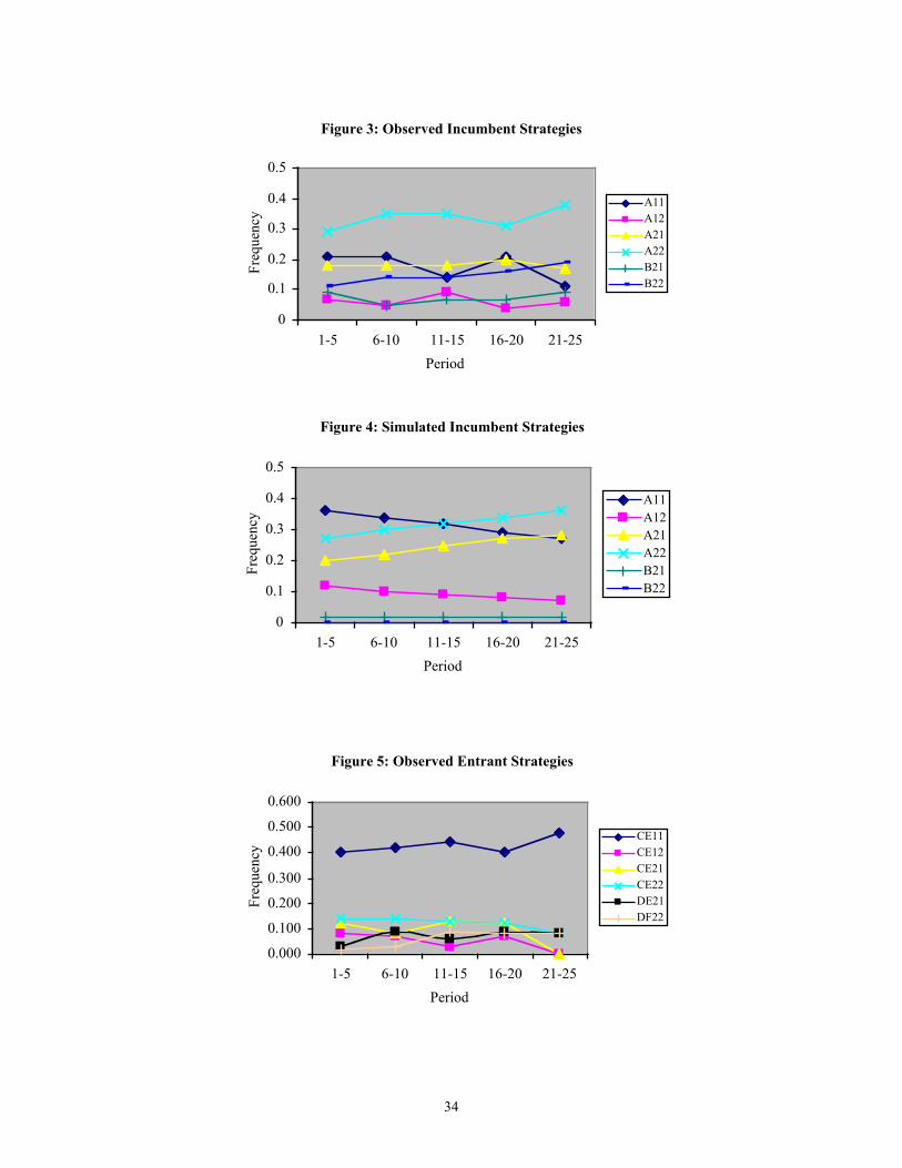
34

Figure 3: Observed Incumbent Strategies

0

0.1

0.2

0.3

0.4

0.5

1-5 6-10 11-15 16-20 21-25

Period

Freq

uenc

y

A11A12A21A22B21B22

Figure 4: Simulated Incumbent Strategies

0

0.1

0.2

0.3

0.4

0.5

1-5 6-10 11-15 16-20 21-25

Period

Freq

uenc

y

A11A12A21A22B21B22

Figure 5: Observed Entrant Strategies

0.000

0.100

0.200

0.300

0.400

0.500

0.600

1-5 6-10 11-15 16-20 21-25

Period

Freq

uenc

y

CE11CE12CE21CE22DE21DF22

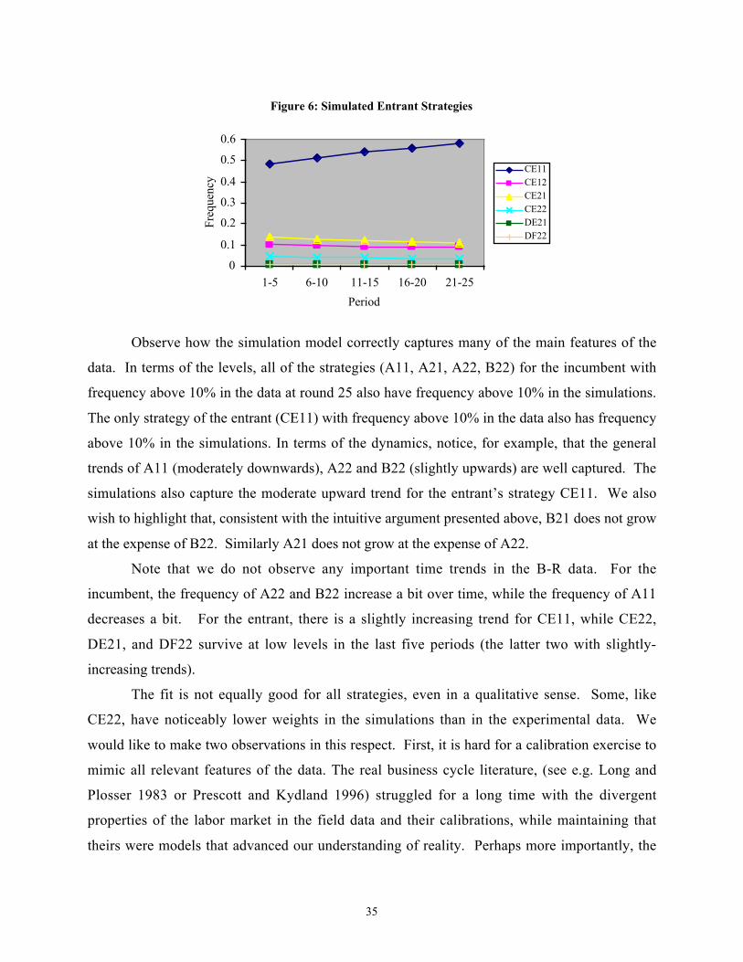
35

Figure 6: Simulated Entrant Strategies

0

0.1

0.2

0.3

0.4

0.5

0.6

1-5 6-10 11-15 16-20 21-25

Period

Freq

uenc

y

CE11CE12CE21CE22DE21DF22

Observe how the simulation model correctly captures many of the main features of the

data. In terms of the levels, all of the strategies (A11, A21, A22, B22) for the incumbent with

frequency above 10% in the data at round 25 also have frequency above 10% in the simulations.

The only strategy of the entrant (CE11) with frequency above 10% in the data also has frequency

above 10% in the simulations. In terms of the dynamics, notice, for example, that the general

trends of A11 (moderately downwards), A22 and B22 (slightly upwards) are well captured. The

simulations also capture the moderate upward trend for the entrant’s strategy CE11. We also

wish to highlight that, consistent with the intuitive argument presented above, B21 does not grow

at the expense of B22. Similarly A21 does not grow at the expense of A22.

Note that we do not observe any important time trends in the B-R data. For the

incumbent, the frequency of A22 and B22 increase a bit over time, while the frequency of A11

decreases a bit. For the entrant, there is a slightly increasing trend for CE11, while CE22,

DE21, and DF22 survive at low levels in the last five periods (the latter two with slightly-

increasing trends).

The fit is not equally good for all strategies, even in a qualitative sense. Some, like

CE22, have noticeably lower weights in the simulations than in the experimental data. We

would like to make two observations in this respect. First, it is hard for a calibration exercise to

mimic all relevant features of the data. The real business cycle literature, (see e.g. Long and

Plosser 1983 or Prescott and Kydland 1996) struggled for a long time with the divergent

properties of the labor market in the field data and their calibrations, while maintaining that

theirs were models that advanced our understanding of reality. Perhaps more importantly, the

36

divergences may highlight avenues for progress. Notice that CE22 is a strategy where player 2

insists in winning the market while refusing to pre-commit. Perhaps some players are simply

showing that they prefer to lose money rather than let others win more than they do. Notice that

it is the strategy with the second lowest average payoffs (Table 6). It would be difficult for a

learning model to capture that effect, which, we must add, is not very large.

In summary, our adaptive learning model demonstrates that the infrequent occurrence of

certain entrant strategies prevents the incumbent from learning which of his own strategies is

dominated. In this way, iteratively weakly-dominated strategies manage to survive over time in

our B-R sessions.

6. DISCUSSION

There is a puzzle in industrial organization: Despite the theoretical arguments advanced

for entry deterrence by incumbents, there is little empirical evidence that firms behave in this

manner. Bagwell and Ramey (1996) propose an alternative model of the timing in the entry

game, in which the ‘first-mover advantage’ disappears through the logic of forward induction.18

They suggest that this is the reason that incumbent firms do not engage in entry deterrence. In

this paper we study behavior in a simplified version of the B-R model and compare it to

observations from a simpler Dixit-style game. We find that in both games the first mover tends

to capture the market, so that the B-R rationale cannot be the key to explaining the entry-

deterrence puzzle.

For the Dixit game the first-mover advantage is predicted by theoretical arguments. In

our data this advantage is strong even when the incumbent does not engage in entry-deterrence;

when the incumbent does pre-install, however, this advantage is substantially more pronounced.

Pre-installation in this game also serves to greatly reduce inefficiency (from the standpoint of the

firms, either zero or two firms in the market) from 32% to 12%.

On the other hand, in the perhaps more realistic B-R environment, theory suggests that

the entrant should have the advantage, as he or she has the final opportunity to pre-install prior to

the choices about market participation. Nevertheless, we find that the incumbent is much more

likely to control the market than the entrant. This advantage is substantial even without

37

incumbent pre-installation, but grows considerably when the first mover pre-installs. Entrant

pre-installation reverses this tendency, as in this case the entrant is much more likely than the

incumbent to control the market. Pre-installation is relatively rare for both the incumbent and the

entrant, and the entrant’s pre-installation has a weaker coordinating effect than the incumbent’s

pre-installation. Solo incumbent pre-installation reduces inefficiency, while solo entrant pre-

installation increases inefficiency.

We go beyond the purely negative implication of our results – the rejection of the B-R

rationalization – and provide an explanation for observed behavior. From the start our data

exhibit a particular pattern which does not disappear as people have the opportunity to learn

through repetition. The question then is why initial behavior is what it is and over time does not

even tend in the direction of the B-R prediction.

The first part of our answer, suggested by some of the regularities that we have just

discussed, is that there is a perceived first-mover advantage in this game. In the B-R game, there

is a large difference in B-R investment rates (72% vs. 36%) when neither player pre-commits;

note also the difference in these rates when only the other player has chosen to pre-install, 51.1%

for the incumbent versus 23.0% for the entrant. The investment rate for incumbents is more than

double the investment rate for entrants in both cases. Thus, for most players the pattern is as if

the incumbent had a ‘natural’ first-mover advantage, something not captured by the strategic

analysis presented above. We also see this in the Dixit game, where an incumbent who does not

pre-install nevertheless is nearly five times as likely to control the market as the entrant.

In the B-R game, the strategy in which the incumbent does not pre-install, but

nevertheless enters the market regardless of the entrant’s pre-installation decision, is by far the

most common (chosen fully 1/3 of the time). The logic of forward induction makes some

inroads against an a priori perception of a first-mover advantage, but generally must surrender to

it – the strategy leading to the highest expected payoff for an entrant in the B-R game involves

always staying out of the market. On the other hand, forward induction and such a perception

work together in the Dixit game, and the incumbent enjoys an overwhelming advantage.

Our answer to the question why the B-R prediction is not held up by our data requires a

second part. Just to posit the existence of a perceived first-mover advantage is not a sufficient

explanation of our data; one must also clarify why learning does not do away with this pre-

18 For a discussion of the Bagwell-Ramey model see also Vives (1999).

38

conception. Our theoretical result with deterministic dynamics and our stochastic simulation

model results provide a rationale for why the initial behavior does not change too much over

time. Thus we feel that we have obtained a rather complete explanation of why the forward-

induction does not win out in our data, despite the clear sensitivity of behavior to the issue of

who has pre-installed. It is not simply based on the notion that people have limitations in their

depth of reasoning. Rather, matters start with a pre-conception that subsequent experience with

the environment is unable to erase.

One may wonder about the origins of a perceived first-mover advantage. Our result bears

relation to some recent experimental findings reported in Weber, Camerer and Knez (2004) and

Muller and Sadanand (2003). These studies show that when simple two-person games that are

‘simultaneous’ in terms of information are played sequentially, the first mover tends to do better

than when both players make actual simultaneous choices. Note that this cannot be explained

just by the fact that the temporal asymmetry in moves allows for better coordination and that

players use any available clue to facilitate coordination. If this were the driving force, then a

second player advantage could arise just as well. There appears to be something special about

moving first.

Huck and Müller (2000) report another instance of a first-mover advantage that

transcends game-theoretic prediction. They study experimentally the Bagwell (1995) result that

the commitment value of moving first is severely undermined if the observability of the earlier

move is even slightly in doubt and find that people do not ignore prior moves even with

imperfect observability.

Our environment is somewhat different since the second mover does observe (at least in

principle) the first mover’s choice. However, perhaps there is something more general in the

psychology of reasoning about timing that favors earlier movers. Weber, Camerer and Knez

(2004) suggest that, consistent with some evidence from psychological experiments, players may

be better at reasoning backward, about events known to have already happened, than reasoning

forward. Description of possible outcomes of previously-occurring events is often richer and

more complex than description of later-occurring events. Weber, Camerer and Knez conjecture

on p.41 that “the past is easier to ‘imagine’ than the future.”

What can we say about the capacity investment puzzle that brought us here? While our

evidence does not support the B-R prediction, it suggests, perhaps paradoxically, that the B-R

39

environment may be the better one to study the matter at hand. Both firms have an opportunity

for capacity investment but neither uses it very much, resulting in a prevailing tendency of

market dominance by the incumbent. While our experimental games are highly stylized, we

believe that our results shed some light on both an important issue in industrial organization and

an interesting topic in behavioral game theory.

REFERENCES

Bagwell, K. (1995), “Commitment and Observability in Games,” Games and EconomicBehavior, 8, 271-280.

Bagwell, K., and G. Ramey (1996), “Capacity, Entry and Forward Induction,” RAND Journal ofEconomics, 27, 660-680.

Bain, J. (1956), Barriers to New Competition, Cambridge, MA: Harvard University Press.Balkenborg, D. (1998), “An Experiment on Forward- versus Backward Induction,” mimeo.Battigalli. P. (1996), “Strategic Rationality Orderings and the Best Rationalization Principle,”

Games and Economic Behavior, 13, 178-200.Basu, K. (1993), “Lectures in Industrial Organization Theory,” Blackwell Publishers: Oxford,

UK.Börgers, T. and R. Sarin (1997), “Learning Through Reinforcement and Replicator Dynamics,”

Journal of Economic Theory, 77, 1-14.Brandts, J. and C. Holt (1995), “Limitations of dominance and forward induction: Experimental

evidence”, Economics Letters, 49, 391-395.Broseta, B., E. Fatás, and T. Neugebauer (2003): “Asset Markets and Equilibrium Selection in

Public Goods Games with Provision Points: An Experimental Study,” Economic Inquiry.Cabrales, A. (2000), “Stochastic Replicator Dynamics,” International Economic Review, 41,

451-481.Camerer, C. and T. Ho (1999), “Experience-Weighted Attraction in Games,” Econometrica, 67,

827-874.Camerer, C. (2003), Behavioral Game Theory, Princeton University Press: Princeton NJ.Cooper, R., D. DeJong, R. Forsythe and T. Ross (1992), “Forward induction in coordination

games”, Economics Letters, 40, 167-172.Cooper, R., D. DeJong, R. Forsythe and T. Ross (1993), “Forward induction in the battle-of-the-

sexes games”, American Economic Review, 83, 1303-1316.Dixit, A. (1980), “The Role of Investment in Entry Deterrence,” Economic Journal, 90, 95-106.Fudenberg, D. and D. Levine (1998), The Theory of Learning in Games, MIT Press, Cambridge

MA.Geroski, P. (1995), “What do we Know about Entry?” International Journal of Industrial

Organization, 13, 421-440.Goeree, J. and C. Holt (2001), “Ten Little Treasures of Game Theory and Ten Intuitive

Contradictions,” American Economic Review, 91, 1402-1422.Hauk, E. and S. Hurkens (2002), “On Forward Induction and Evolutionary and Strategic

Stability,” Journal of Economic Theory, 106, 66-90.

40

Huck, S. and W. Müller (2000), “Perfect versus imperfect observability – An experimental testof Bagwell’s result,” Games and Economic Behavior, 31, 174-190.

Kohlberg, E. and J.-F. Mertens (1986), “On the Strategic Stability of Equilibrium,”Econometrica, 54, 1003-1038.

Long, J. Jr., and C. Plosser (1983), “Real Business Cycles,” Journal of Political Economy, 91,39-69.

Martin, Stephen (1993), Advanced Industrial Economics, Basil Blackwell.Mason, C.F. and C. Nowell (1998), “An experimental analysis of subgame perfect play: the entry

deterrence game,” Journal of Economic Behavior and Organization, 37, 443-462.McKelvey, R.M. and T.R. Palfrey (1995), “Quantal Response Equilibria in Normal Form

Games,” Games and Economic Behavior, 7, 6-38.Modigliani, F. (1958), “New developments on the oligopoly front”, Journal of Political

Economy, 66, 215-232.Muller, R. and A. Sadanand (2003), “Order of Play, Forward Induction, and Presentation Effects

in Two-Person Games”, Experimental Economics, 6, 5-25.Prescott, E. and F. Kydland (1996), “The Computational Experiment: An Econometric Tool,”

Journal of Economic Perspectives , 10, 69-85.Samuelson, L. (1997), Evolutionary Games and Equilibrium Selection, MIT Press: Cambridge

MA.Schotter, A., K. Weigelt and C. Wilson (1994), “ A laboratory investigation of multiperson

rationality and presentation effects,” Games and Economic Behavior, 6, 445-468.Siegel, S. and N. Castellan, Jr. (1988), Nonparametric Statistics for the Behavioral Sciences,

Boston: McGraw-Hill.Singh, S., M. Utton and M. Waterson (1998), “Strategic Behavior of Incumbent Firms in the

U.K.,” International Journal of Industrial Organization, 16, 229-251.Smiley, R. (1988), “Empirical Evidence on Strategic Entry Deterrence,” International Journal of

Industrial Organization, 6, 167-180.Tirole, J. (1989), The Theory of Industrial Organization, MIT Press: Cambridge MA.Van Damme, E. (1989), “Stable Equilibria and Forward Induction,” Journal of Economic

Theory, 48, 476-496.Van Huyck, J., R. Battalio and R. Beil (1993), “Asset markets as an equilibrium selection

mechanism: Coordination failure, game form auctions, and tacit communication,” Gamesand Economic Behavior, 5, 485-504.

Vives, X. (1999), Oligopoly Pricing: Old Ideas and New Tools, MIT Press: Cambridge MA.Vega-Redondo, F. (1996), Evolution, Games and Economic Behavior, Oxford University Press:

Oxford, UK.Weber, R., C. Camerer and Marc Knez (2004), “Timing and Virtual Observability in Ultimatum

Games and ‘Weak Link’ Coordination Games,” Experimental Economics, 7, 25-48.

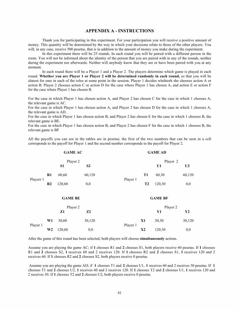
41

APPENDIX A - INSTRUCTIONS

Thank you for participating in this experiment. For your participation you will receive a positive amount ofmoney. This quantity will be determined by the way in which your decisions relate to those of the other players. Youwill, in any case, receive 500 pesetas, that is in addition to the amount of money you make during the experiment.

In this experiment there will be 25 rounds. In each round you will be paired with a different person in theroom. You will not be informed about the identity of the person that you are paired with in any of the rounds, neitherduring the experiment nor afterwards. Neither will anybody know that they are or have been paired with you at anymoment.

In each round there will be a Player 1 and a Player 2. The players determine which game is played in eachround. Whether you are Player 1 or Player 2 will be determined randomly in each round, so that you will bealmost for sure in each of the roles at some point in the session. Player 1 decides whehterh she chooses action A oraction B. Player 2 chooses action C or action D for the case where Player 1 has chosen A, and action E or action Ffor the case where Player 1 has chosen B.

For the case in which Player 1 has chosen action A, and Player 2 has chosen C for the case in which 1 chooses A,the relevant game is AC.For the case in which Player 1 has chosen action A, and Player 2 has chosen D for the case in which 1 chooses A,the relevant game is AD.For the case in which Player 1 has chosen action B, and Player 2 has chosen E for the case in which 1 chooses B, therelevant game is BE.For the case in which Player 1 has chosen action B, and Player 2 has chosen F for the case in which 1 chooses B, therelevant game is BF

All the payoffs you can see in the tables are in pesetas; the first of the two numbers that can be seen in a cellcorresponds to the payoff for Player 1 and the second number corresponds to the payoff for Player 2.

GAME AC GAME AD

Player 2 Player 2 S1 S2 U1 U2

R1 60,60 60,120 T1 60,30 60,120 Playerr 1 Player 1

R2 120,60 0,0 T2 120,30 0,0

GAME BE GAME BF

Player 2 Player 2 Z1 Z2 Y1 Y2

W1 30,60 30,120 X1 30,30 30,120 Player 1 Player 1

W2 120,60 0,0 X2 120,30 0,0

After the game of this round has been selected, both players will choose simultaneously actions.

Assume you are playing the game AC; if 1 chooses R1 and 2 chooses S1, both players receive 60 pesetas. If 1 choosesR1 and 2 chooses S2, 1 receives 60 and 2 receives 120. If 1 chooses R2 and 2 chooses S1, 1 receives 120 and 2receives 60. If 1 chooses R2 and 2 chooses S2, both players receive 0 pesetas.

Assume you are playing the game AD; if 1 chooses T1 and 2 chooses U1, 1 receives 60 and 2 receives 30 pesetas. If 1chooses T1 and 2 chooses U2, 1 receives 60 and 2 receives 120. If 1 chooses T2 and 2 chooses U1, 1 receives 120 and2 receives 30. If 1 chooses T2 and 2 chooses U2, both players receive 0 pesetas.

42

Assume you are playing the game BE; if 1 chooses W1 and 2 chooses Z1, 1 receives 30 and 2 receives 60 pesetas. If 1chooses W1 and 2 chooses Z2, 1 receives 30 and 2 receives 120. If 1 chooses W2 and 2 chooses Z1, 1 receives 120 and2 receives 60. If 1 chooses W2 and 2 chooses Z2, both players receive 0 pesetas.

Assume you are playing the game BF; if 1 chooses X1 and 2 chooses Y1, both players receive 30 pesetas. If 1 choosesX1 and 2 chooses Y2, 1 receives 30 and 2 receives 120. If 1 chooses X2 and 2 chooses Y1, 1 receives 120 and 2receives 30. If 1 chooses X2 and 2 chooses Y2, both players receive 0 pesetas.

Development of the session

1) At the beginning of the game each person was given a piece of paper. In the row corresponding to each round, thecolumn 1 indicates if in that round you are Player 1 or Player 2.

2) Each Player 1 has to mark in her decision sheet her decision about the game to play: A or B, in column 2.3) Each Player 2 has to mark in column 3 her decision (C or D) for the case in which Player 1 has chosen A, and in

column 4 her decision (E or F) for the case in which Player 1 has chosen B. That is, Player 2 must make twodecisions at this point.

Choice of actions in the game: Once you have made the decisions about which game to play (that is, the decisions towhich we refer at points 2) or 3)), you also must make the decisions in the possible games that will result, which willbe two in all cases. That is:

1) Each Player 1 who has decided to use the action A, must choose which action (R1 or R2) to take if the gameis finally AC (in column 5) and which action (T1 or T2) to take if the game is finally AD (in column 6).

2) Each Player 1 who has decided to use the action B, must choose which action (W1 or W2) to take if the gameis finally BE (in column 7) and which action (X1 or X2) she will take if the game is finally BF (in column 8).

3) Each Player 2 who has decided to use the action C in case of A and E in case of B, must choose which action(S1 or S2) to take if the game is finally AC (in column 5) and which action (Z1 or Z2) to take if the game isfinally BE (in column 7).

4) Each Player 2 who has decided to use the action C in case of A and F in case of B, must choose which action(S1 or S2) to take if the game is finally AC (in column 5) and which action (Y1 or Y2) to take if the game isfinally BF (in column 8).

5) Each Player 2 who has decided to use the action D in case of A and E in case of B, must choose which action(U1 or U2) to take if the game is finally AD (in column 6) and which action (Z1 or Z2) to take if the game isfinally BE (in column 7).

6) Each Player 2 who has decided to use the action D in case of A and F in case of B, must choose which action(U1 or U2) to take if the game is finally AD (in column 6) and which action (Y1 or Y2) to take if the game isfinally BF (in column 8).

When you have all taken your decisions for a round, a monitor will pass through the classroom writing them down andafter in column 9 you will be informed of the strategy of the other player. During the first 5 rounds you will beinformed about the final result, in column 10. With this information and the payoff tables you have in theseinstructions you can calculate the final result (from round 6) and your payoffs (all rounds), which you will write downrespectively in columns 10 and 11.

Please make your decisions one by one. The information we give you after every round (including the informationindicating what would have happened in a game different from the one finally played) can be of help to take yourdecision.

Payment: At the end of the 25 rounds, the payoffs of each person will be added up and each one will receive herpayoffs one by one and in private. After the beginning of the experiment there can be no communication between theparticipants. Please, if you have any questions, now or during the experiment, raise your hand and a monitor willrespond. Are there any questions?.

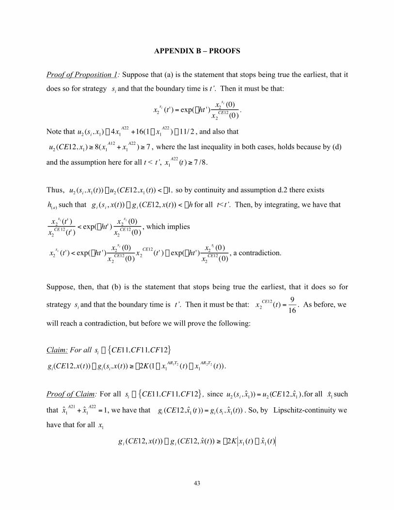
43

APPENDIX B – PROOFS

Proof of Proposition 1: Suppose that (a) is the statement that stops being true the earliest, that it

does so for strategy is and that the boundary time is t’. Then it must be that:

†

x2si (t ') = exp(-ht ') x2

si (0)x2

CE12(0).

Note that

†

u2 (si , x1) £ 4x1A22

+16(1- x1A22 ) £11/ 2 , and also that

†

u2 (CE12, x1) ≥ 8(x1A12

+ x1A22 ) ≥ 7 , where the last inequality in both cases, holds because by (d)

and the assumption here for all t < t’,

†

x1A22 (t ) ≥ 7 /8.

Thus,

†

u2 (si , x1(t)) -u2 (CE12,x1 (t)) < -1, so by continuity and assumption d.2 there exists

)(ah such that htxCEgtxsg iii -<- ))(,12())(,( for all t<t’. Then, by integrating, we have that

†

x2si (t ' )

x2CE 12(t' )

< exp(-ht' ) x2si (0)

x2CE 12(0)

, which implies

†

x2si (t ') < exp(-ht ') x2

si (0)x2

CE12(0)x2

CE12(t ' ) £ exp(-ht ') x2si (0)

x2CE12(0)

, a contradiction.

Suppose, then, that (b) is the statement that stops being true the earliest, that it does so for

strategy is and that the boundary time is t’. Then it must be that:

†

x2CE12(t) =

916

. As before, we

will reach a contradiction, but before we will prove the following:

Claim: For all

†

si ΠCE11,CF11,CF12{ }

†

gi(CE12, x(t)) - gi(si, x(t)) ≥ -2K(1- x1AR1T2 (t) - x1

AR2T2 (t)).

Proof of Claim: For all

†

si ΠCE11,CF11,CF12{ } , since

†

u2 (si , ˆ x 1)) = u2 (CE12, ˆ x 1 ),for all 1̂x such

that

†

ˆ x 1A21

+ ˆ x 1A22

=1, we have that

†

gi (CE12, ˆ x 1 (t )) = gi(si , ˆ x 1(t)) . So, by Lipschitz-continuity we

have that for all 1x

)(ˆ)(2))(ˆ,12())(,12( 11 txtxKtxCEgtxCEg ii --≥-

44

)(ˆ)(2))(,())(ˆ,( 11 txtxKtxsgtxsg iiii --≥-

But since ))(ˆ,())(ˆ,12( txsgtxCEg iii = , adding the previous two inequalities yields the result.�

Now, by the claim, ))()(1(2))(,())(,12( 221

121 txtxKtxsgtxCEg AA

iii ---≥- , but by

assumption, for all t<t’

†

x1si (t) < exp(-h(c)t)

x1si (0)

x1A22(0)

for all

†

si œ A21, A22{ } so that

{ } ))0(

)0(

)(exp(2))(,())(,12(22

1

22,211

)( A

AAs

s

ciiix

x

thKtxsgtxCEg i

iÂœ--≥- . Then by integration we have that

†

x2CE 12(t ')

x2CE12(0)

x2si (0)

x2si (t ')

> 2 Kh(c)

x1si (0)

si œ A21,A 22{ }Â

x1A22 (0)

≥ 2 Kh(c)

. This implies that

†

x2CE 12(t ')

x2CE12(0)

> 2 Kh(c)

x2si (t ')

x2si (0)

, and by summing over all

†

si Œ S2* ≡ CE11,CE12,CF11,CF12{ } we have

that:

†

x2CE 12(t ')

x2CE12(0)

> 2 Kh

x2si (t ')

si ŒS2*

Â

Maxsi ΠS2

* x2si (0)

= 2 Kh

1- x2si (t ')

si œS2*

Â

x2si (0)

≥ 2 Kh

1-x2

si (0)x2

CE 12(0)si œS2*

Â

Maxsi ΠS2

* x2si (0)

where the last inequality is true by (a). This yields a contradiction by the assumption about the

initial conditions.

Suppose that (c) is the statement that stops being true the earliest, that it does so for strategy

is and that the boundary time is t’. Then it must be that:

†

x1si (t ') = exp(-h(c)t ')

x1si (0)

x1A22(0)

.

Note that

†

u1(si , x1) £16(1- x2CF12 ) £ 7 and also that

†

u1(A22, x1) ≥16x2CF12

≥ 9 , where the last

inequality in both cases, holds because by (d) and the assumption here for all t < t’,

†

x1CF 22(t ) ≥ 9/16.

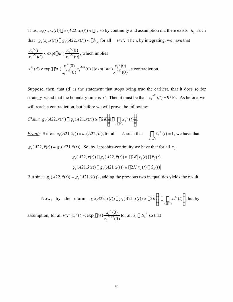
45

Thus,

†

u1(si , x2 (t)) -u1 (A22, x2 (t)) < -1, so by continuity and assumption d.2 there exists )(ah such

that )())(,22())(,( aiii htxAgtxsg -<- for all t<t’. Then, by integrating, we have that

†

x1si (t ' )

x1A22 (t ')

< exp(-ht' ) x1si (0)

x1A22 (0)

, which implies

†

x1si (t ') < exp(-ht ') x1

si (0)x1

A22(0)x1

A22(t ') £ exp(-ht ' ) x1si (0)

x1A22 (0)

, a contradiction.

Suppose, then, that (d) is the statement that stops being true the earliest, that it does so for

strategy is and that the boundary time is t’. Then it must be that

†

x1A22 (t ') = 9/16. As before, we

will reach a contradiction, but before we will prove the following:

Claim: ˜˜¯

ˆÁÁË

Ê--≥- Â

Œ

)(12))(,21())(,22(2

*2 txKtxAgtxAg

Ss

sii

i

i .

Proof: Since

†

u1(A21, ˆ x 2 )) = u2 (A22, ˆ x 2 ), for all 2x̂ such that 1)(ˆ2

*2 =Â

Œ

txSs

s

i

i , we have that

))(ˆ,21())(ˆ,22( txAgtxAg ii = . So, by Lipschitz-continuity we have that for all 2x

)(ˆ)(2))(ˆ,22())(,22( 22 txtxKtxAgtxAg ii --≥-

)(ˆ)(2))(,21())(ˆ,21( 22 txtxKtxAgtxAg ii --≥-

But since ))(ˆ,21())(ˆ,22( txAgtxAg ii = , adding the previous two inequalities yields the result.�

Now, by the claim, ˜˜¯

ˆÁÁË

Ê--≥- Â

Œ

)(12))(,21())(,22(2

*2 txKtxAgtxAg

Ss

sii

i

i , but by

assumption, for all t<t’

†

x2si (t) < exp(-ht ) x2

si (0)x2

CE12(0)for all *

2Ssi œ so that

46

˜̃˜˜

¯

ˆ

ÁÁÁÁ

Ë

Ê

--≥-Âœ

)0(

)0(

)exp(2))(,21())(,22(12

2

2*

2

CE

Ss

s

iix

x

htKtxAgtxAg i

i

. Then, by integration we have that

†

x1A22 (t ')

x1A22 (0)

x1A22 (0)

x1A22(t' )

> 2 Kh

x2si (0)

si œS2*

Â

x2CE 12(0)

≥ 2 Kh

. This implies that

†

x1A22 (t ')

x1A22 (0)

> 2 Kh

x1A21(t ')

x1A21(0)

. By adding

up over all

†

si ΠA21, A22{ } we have that

†

x1A22 (t ')

x1A22 (0)

>Kh

x1si (t ' )

si ΠA 21,A 22{ }

Â

MaxsiΠA21,A22{ }x1si (0)

= 2 Kh

1- x1si (t ')

siœ A 21, A22{ }

Â

Maxsi ΠA21, A22{ }x1si (0)

≥ 2 Kh

1-x1

si (0)x1

A22 (0)siœ A 21, A 22{ }

Â

Maxsi ΠA21,A22{ }x1si (0)

,

where the last inequality is true by (c). This yields a contradiction by the assumption about the

initial conditions.

Since this exhausts all cases the result follows.

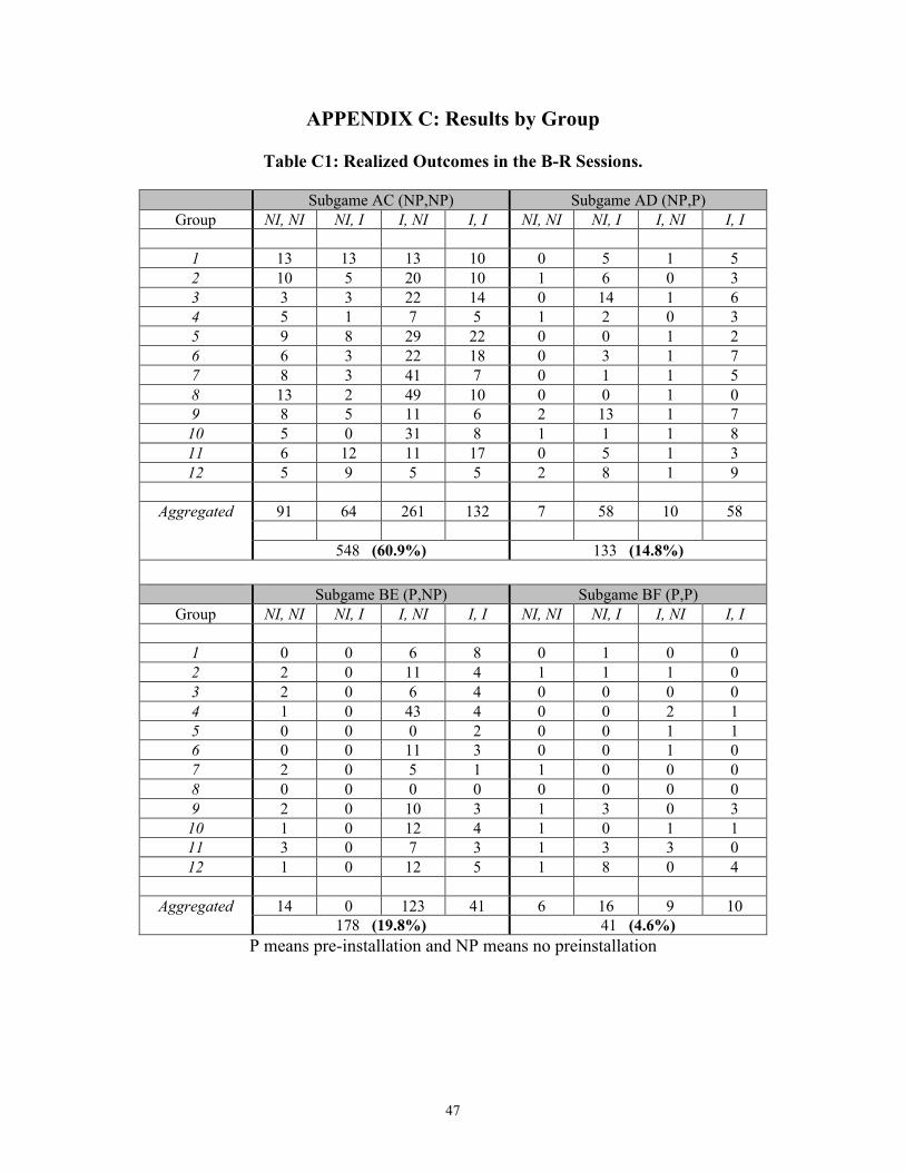
47

APPENDIX C: Results by Group

Table C1: Realized Outcomes in the B-R Sessions.

Subgame AC (NP,NP) Subgame AD (NP,P)Group NI, NI NI, I I, NI I, I NI, NI NI, I I, NI I, I

1 13 13 13 10 0 5 1 52 10 5 20 10 1 6 0 33 3 3 22 14 0 14 1 64 5 1 7 5 1 2 0 35 9 8 29 22 0 0 1 26 6 3 22 18 0 3 1 77 8 3 41 7 0 1 1 58 13 2 49 10 0 0 1 09 8 5 11 6 2 13 1 710 5 0 31 8 1 1 1 811 6 12 11 17 0 5 1 312 5 9 5 5 2 8 1 9

91 64 261 132 7 58 10 58Aggregated

548 (60.9%) 133 (14.8%)

Subgame BE (P,NP) Subgame BF (P,P)Group NI, NI NI, I I, NI I, I NI, NI NI, I I, NI I, I

1 0 0 6 8 0 1 0 02 2 0 11 4 1 1 1 03 2 0 6 4 0 0 0 04 1 0 43 4 0 0 2 15 0 0 0 2 0 0 1 16 0 0 11 3 0 0 1 07 2 0 5 1 1 0 0 08 0 0 0 0 0 0 0 09 2 0 10 3 1 3 0 310 1 0 12 4 1 0 1 111 3 0 7 3 1 3 3 012 1 0 12 5 1 8 0 4

14 0 123 41 6 16 9 10Aggregated178 (19.8%) 41 (4.6%)

P means pre-installation and NP means no preinstallation

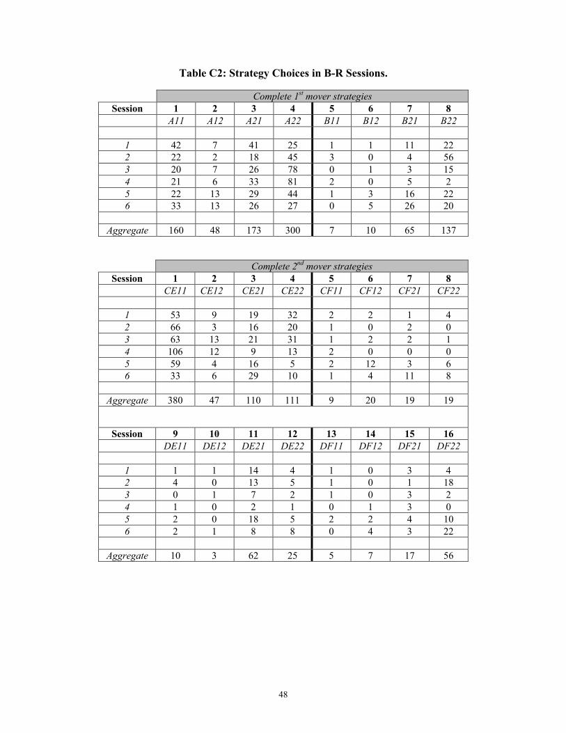
48

Table C2: Strategy Choices in B-R Sessions.

Complete 1st mover strategiesSession 1 2 3 4 5 6 7 8

A11 A12 A21 A22 B11 B12 B21 B22

1 42 7 41 25 1 1 11 222 22 2 18 45 3 0 4 563 20 7 26 78 0 1 3 154 21 6 33 81 2 0 5 25 22 13 29 44 1 3 16 226 33 13 26 27 0 5 26 20

Aggregate 160 48 173 300 7 10 65 137

Complete 2nd mover strategiesSession 1 2 3 4 5 6 7 8

CE11 CE12 CE21 CE22 CF11 CF12 CF21 CF22

1 53 9 19 32 2 2 1 42 66 3 16 20 1 0 2 03 63 13 21 31 1 2 2 14 106 12 9 13 2 0 0 05 59 4 16 5 2 12 3 66 33 6 29 10 1 4 11 8

Aggregate 380 47 110 111 9 20 19 19

Session 9 10 11 12 13 14 15 16DE11 DE12 DE21 DE22 DF11 DF12 DF21 DF22

1 1 1 14 4 1 0 3 42 4 0 13 5 1 0 1 183 0 1 7 2 1 0 3 24 1 0 2 1 0 1 3 05 2 0 18 5 2 2 4 106 2 1 8 8 0 4 3 22

Aggregate 10 3 62 25 5 7 17 56

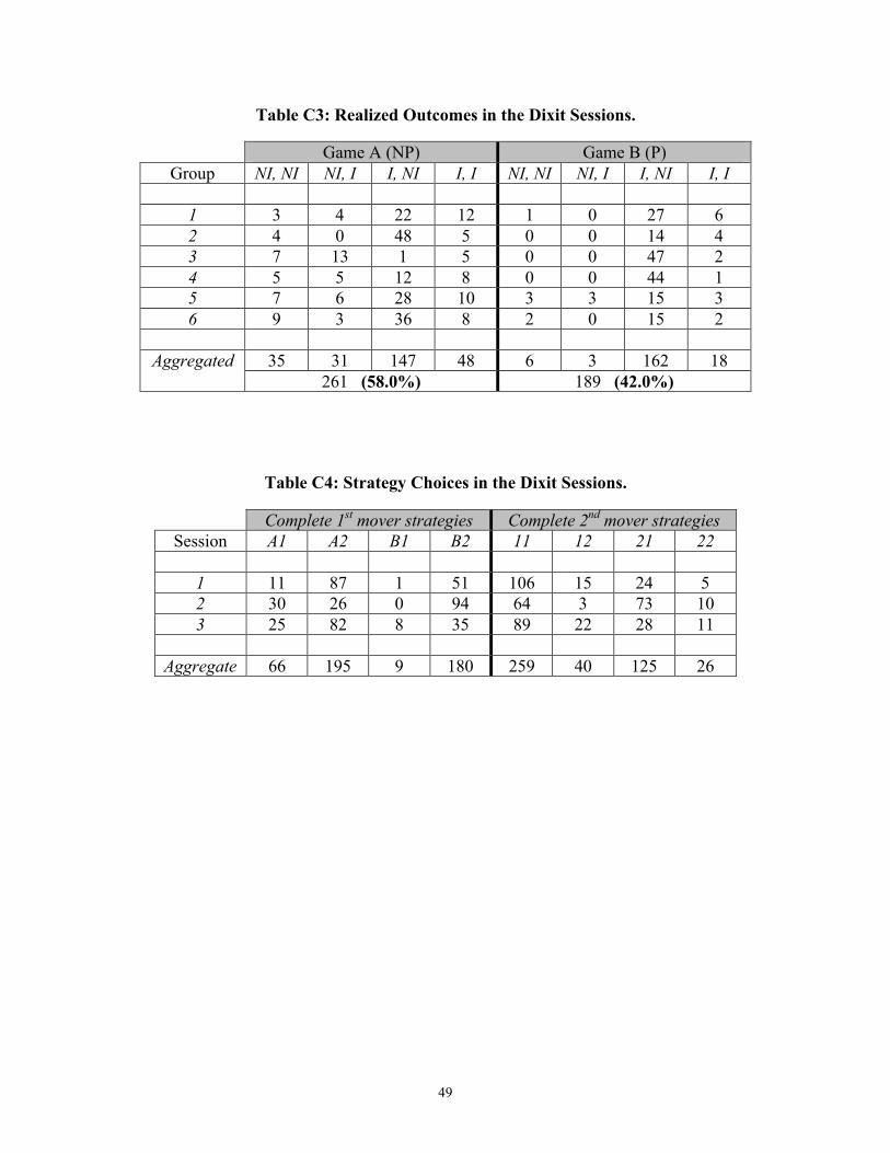
49

Table C3: Realized Outcomes in the Dixit Sessions.

Game A (NP) Game B (P)Group NI, NI NI, I I, NI I, I NI, NI NI, I I, NI I, I

1 3 4 22 12 1 0 27 62 4 0 48 5 0 0 14 43 7 13 1 5 0 0 47 24 5 5 12 8 0 0 44 15 7 6 28 10 3 3 15 36 9 3 36 8 2 0 15 2

35 31 147 48 6 3 162 18Aggregated261 (58.0%) 189 (42.0%)

Table C4: Strategy Choices in the Dixit Sessions.

Complete 1st mover strategies Complete 2nd mover strategiesSession A1 A2 B1 B2 11 12 21 22

1 11 87 1 51 106 15 24 52 30 26 0 94 64 3 73 103 25 82 8 35 89 22 28 11

Aggregate 66 195 9 180 259 40 125 26

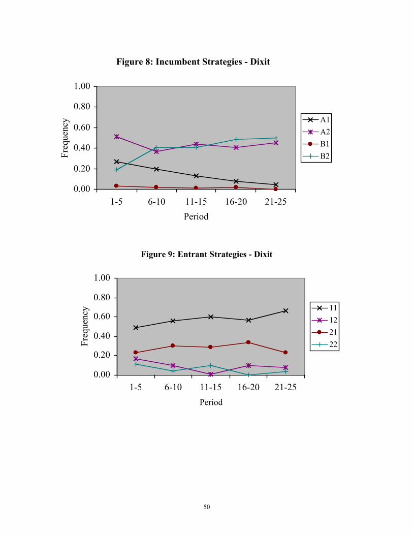
50

Figure 8: Incumbent Strategies - Dixit

0.00

0.20

0.40

0.60

0.80

1.00

1-5 6-10 11-15 16-20 21-25

Period

Freq

uenc

y A1

A2

B1

B2

Figure 9: Entrant Strategies - Dixit

0.00

0.20

0.40

0.60

0.80

1.00

1-5 6-10 11-15 16-20 21-25

Period

Freq

uenc

y 11

12

21

22