enhancing usability of the multi-channel analysis of
TRANSCRIPT

University of Tennessee, Knoxville University of Tennessee, Knoxville
TRACE: Tennessee Research and Creative TRACE: Tennessee Research and Creative
Exchange Exchange
Doctoral Dissertations Graduate School
12-2013
Enhancing Usability of the Multi-channel Analysis of Surface Enhancing Usability of the Multi-channel Analysis of Surface
Wave (MASW) Technique for Subsurface Physical Property Wave (MASW) Technique for Subsurface Physical Property
Mapping by Incorporating Random-Array Seismic Acquisition Mapping by Incorporating Random-Array Seismic Acquisition
Prasanta Malati Yeluru University of Tennessee - Knoxville, [email protected]
Follow this and additional works at: https://trace.tennessee.edu/utk_graddiss
Part of the Geophysics and Seismology Commons
Recommended Citation Recommended Citation Yeluru, Prasanta Malati, "Enhancing Usability of the Multi-channel Analysis of Surface Wave (MASW) Technique for Subsurface Physical Property Mapping by Incorporating Random-Array Seismic Acquisition. " PhD diss., University of Tennessee, 2013. https://trace.tennessee.edu/utk_graddiss/2634
This Dissertation is brought to you for free and open access by the Graduate School at TRACE: Tennessee Research and Creative Exchange. It has been accepted for inclusion in Doctoral Dissertations by an authorized administrator of TRACE: Tennessee Research and Creative Exchange. For more information, please contact [email protected].

To the Graduate Council:
I am submitting herewith a dissertation written by Prasanta Malati Yeluru entitled "Enhancing
Usability of the Multi-channel Analysis of Surface Wave (MASW) Technique for Subsurface
Physical Property Mapping by Incorporating Random-Array Seismic Acquisition." I have
examined the final electronic copy of this dissertation for form and content and recommend
that it be accepted in partial fulfillment of the requirements for the degree of Doctor of
Philosophy, with a major in Geology.
Gregory S. Baker, Major Professor
We have read this dissertation and recommend its acceptance:
Edmund Perfect, Larry Taylor, Dayakar Penumadu
Accepted for the Council:
Carolyn R. Hodges
Vice Provost and Dean of the Graduate School
(Original signatures are on file with official student records.)

Enhancing Usability of the Multi-channel Analysis of Surface Wave (MASW)
Technique for Subsurface Physical Property Mapping by Incorporating
Random-Array Seismic Acquisition
A Dissertation Presented for the
Doctor of Philosophy
Degree
The University of Tennessee, Knoxville
Prasanta Malati Yeluru
December 2013

ii
DEDICATION
To my husband, daughter and family
iii
ACKNOWLEDGMENTS
I would like to express my sincere gratitude to my advisor, Dr. Gregory S Baker for
giving me the opportunity to perform the degree and also for his guidance and support during my
doctoral studies. I have benefited tremendously from his experience and clear thought in the
research. He has provided for me not only his knowledge but also his deep and kind
consideration.
I would like to thank the other members of my committee, Dr. Ed Perfect, Dr. Larry
Taylor and Dr. Dayakar Penumadu for their valuable comments and suggestions.
I would also like to thank: Dr. Choon Park for passing to me much of his knowledge of
surface wave methods; Dr. George McMechan, University of Texas-Dallas for his ultimate
support and for providing me with access to work in his lab; Megan Carr, David Gaines, Rachel
Storniolo, Caitlyn Williams and Matt Edmunds for their friendships.
I am deeply indebted to my parents, parents-in-law, and family for their patience,
understanding and encouragement. I would like to thank my husband, Phaniveer Koti and
daughter, Snigdha Lahari Koti for their love, support, encouragement and smile during this
difficult time. They have made this possible.
And most of all, I thank the almighty for His countless blessings bestowed upon me and
guided me throughout my educational journey.
iv
ABSTRACT
Subsurface imaging is very critical to exploit subsurface resources, monitor the fluid movement
in the reservoir, mapping tunnels etc. As science advances scientists and other researchers are
constantly trying to develop new techniques and methods for subsurface imaging that are more
effective, efficient, and are more robust under varying field conditions. The main focus of this
research is one such effort to improve and increase the usability of the Multi-channel Analysis of
Surface Wave method (MASW) method in determining regolith and rock properties by
introducing a new type of receiver arrangement to extend its usage in places that are inaccessible
for example, near embankments, military places, clandestine burials, etc. Advances in near-
surface geophysical techniques, such as multi-channel analysis of surface waves (MASW), have
greatly increased our ability to map subsurface variations in physical properties here on Earth.
The MASW method involves deployment of multiple seismometers to acquire 1-D or 2-D shear
wave velocity profiles that can be directly related to various engineering properties. The purpose
of the research presented here is to demonstrate the usefulness and capabilities of MASW
technique using a random receiver array 1) through controlled site experiments, 2) through
Modeling experiments, and 3) And finally apply the technique at terrestrial site (the Black Point
Lava Flow) with a different geologic setting. The results focus on near-surface MASW studies
and interpretation of the subsurface geology using a random geophone array. The field
techniques and methodologies discussed in this dissertation, although applicable on Earth, are
also intended for surfaces and regolith in the future exploration of planetary bodies for possible
human habitation. This would include Mars, its Moon-Phobus/Deimos, Near-Earth Asteroids
(NEA’s), even Earth’s Moon. With each situation, the nature of the regolith and its formational
processes will place certain restrictions and limitations upon the applications. This is expected
with any change of terrains even on the Earth, let alone between planetary bodies.
v
TABLE OF CONTENTS
Chapter 1: Introduction 1
1.1 Motivation 2
1.2 Research Objectives 3
1.3 Dissertation Outline 5
1.4 Significance of Study 6
Chapter 2: Overview of Surface Wave Theory 7
2.1 Introduction 8
2.2 Rayleigh Waves in Layered Media 8
2.2.1 Dispersion Equation 10
2.2.2 Phase Velocities of Rayleigh Waves 11
2.3 Surface Wave Theory 13
2.4 Overall MASW Procedure 14
2.4.1 Field procedure-Data Acquisition 15
2.4.2 Field procedure-Data Analysis 20
2.4.3 Field procedure-Data Inversion 21
2.5 Summary 24
Chapter 3: Exploring Multi-channel Analysis of Surface Waves with Random receiver
Arrays for Planetary Exploration 25
Abstract 26
3.1 Introduction 27
3.2 Overview of MASW Method 28
3.3 MASW Data Collected for Random Receiver Arrays 30
3.4 MASW Data Acquired from Linear Receiver Arrays 35
3.5 Visual Analysis of Dispersion Curves 40
3.6 Statistical Analysis of the test data 42
3.7 Discussions and Conclusions 47
Chapter 4: Forward Modeling Experiments for Dispersion Curve Resolution Pertaining
to Random Array MASW 49
Abstract 50
4.1 Introduction 51
4.2 Modeling Program Overview 53
4.3 Theory of Surface Wave Properties 54
4.4 Considerations for Numerical Simulations 56
4.5 Group vs. Phase Velocity Assumptions 57
4.6 Modeling of Typical Regolith Profiles 58
4.7 Analytical Considerations for Dispersion Curve Analysis 60
4.8 Modeling Results 64
4.8.1 Clustered Array Results 64
4.8.2 Skewness Effect 68
4.8.3 Total Number of Traces 70

vi
4.8 Discussion 73
4.9 Conclusions 73
Chapter 5: Comparison of Seismic Surface Wave Dispersion Results Obtained from
Conventional Versus Random Receiver Arrays 74
Abstract 76
5.1 Introduction 76
5.2 Site Description-Geologic Setting 77
5.3 Data Acquisition and Analysis 79
5.4 Linear data processing in 2D format 93
5.5 Results 97
5.6 Statistical Analysis 103
5.6 Conclusions 104
Chapter 6: Adapting a Random-Array Acquisition Scheme For A Seismic Surface-Wave
Study of a Terrestrial Analog Site At Black Point Lava Flow, Arizona USA,
As A Potential Rover-Friendly Methodology 106
Abstract 107
6.1 Introduction 108
6.2 Terrestrial Analog Sites for Seismic Studies 109
6.3 Geologic Setting-Black Point Lava Flow Site 111
6.4 Field Test Procedure 113
8.4.1 Data Acquisition 114
8.4.2 Data Analysis-Dispersion 116
8.4.3 Data Analysis-Inversion 119
8.4.4 Data Interpretation 121
6.5 Statistical Analysis 123
6.6 Conclusions 126
Chapter 7: Summary, Conclusions and Future Work 129
7.1 Summary and Conclusions 130
7.1.1 Random Array Analysis 131
7.1.2 Comparison of Various Geophone Arrays 132
7.1.3 Forward Modeling Experiments 132
7.1.4 Application of Random Array MASW 133
7.2 Overall Conclusions and Implication of Research 134
7.3 Future Work 135
References 136
Appendices 145
Vita 177

vii
LIST OF TABLES
Table 1 Data acquisition parameters for active survey (modified from
www.masw.com)
19
Table 2 Summary of data acquisition parameters 33
Table 3 Statistical parameters used in Kriging method 45
Table 4 A layered earth model parameters chosen from the dispersion curve
obtained from the field data
57
Table 5 Model for a homogeneous half space 59
Table 6 Model for regular regolith profile with stiffness of layers increasing
with depth
59
Table 7 Model for irregular regolith profile with a soft layer trapped between
two stiff layers
59
Table 8 Model for irregular regolith profile with stiff layer trapped between
two soft layers
60
Table 9 Longest wavelength (λmax) and corresponding approximate depth of
investigation (Zmax) calculated for each type of configuration
68
Table 10 Parameters as used in the field for different receiver arrays 81
Table 11 Statistical (mixed model analysis) analysis performed on inversion
data using SAS programming with dependent variable Vs (shear-wave
velocity).
105
Table 12 Summary of data acquisition parameters
116
Table 13
Statistical (mixed model) analysis performed on inversion data using
SAS programming with dependent variable Vs (shear-wave velocity)
124
Table 14 Dynamic properties of regolith layers with depth at BPLF site
measured using MASW method
126

viii
LIST OF FIGURES
Figure 1 Vertical particle motions of two Rayleigh waves with different
wavelengths (Rix, 2000). 11
Figure 2
Schematic representation of the active MASW field survey (modified
from Park, 2003).
16
Figure 3
Typical multichannel seismic surface-wave experiment setup and
MASW data processing procedure (modified from Park, 1999).
29
Figure 4
The figure on the left represents the shot point locations as deployed on
the ground. There are total 13 shot points (shown as s1, s2, etc.) from
which data was collected. The distance between each shot point location
is 10 m. The figure on the right represents the random arrangement of
geophones (small circles) inside a 10 m×10 m grid.
32
Figure 5
Selected data (shot gathers) acquired from a field test site in the
University of Tennessee agricultural center, Knoxville, Tennessee, with
48-channel system and their corresponding dispersion images.
34
Figure 6
Linear raw field data showing some bad traces which may have occurred
due to geophone polarity issues or the way they were installed, poor type
of source used/coupling, or some malfunctioning of geophones.
36
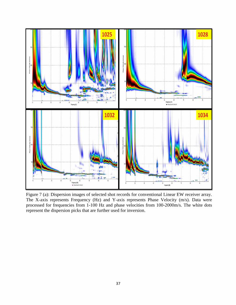
Figure 7
(a) Dispersion images of selected shot records for conventional Linear
EW receiver array. The X-axis represents Frequency (Hz) and Y-axis
represents Phase Velocity (m/s). Data were processed for frequencies
from 1-100 Hz and phase velocities from 100-2000m/s. The white dots
represent the dispersion picks that are further used for inversion. (b)
Dispersion images of selected shot records for conventional Linear NS
receiver array. The X-axis represents Frequency (Hz) and Y-axis
represents Phase Velocity (m/s). Data were processed for frequencies
from 1-100 Hz and phase velocities from 100-2000m/s. The white dots
represent the dispersion picks that are further used for inversion.
37,38
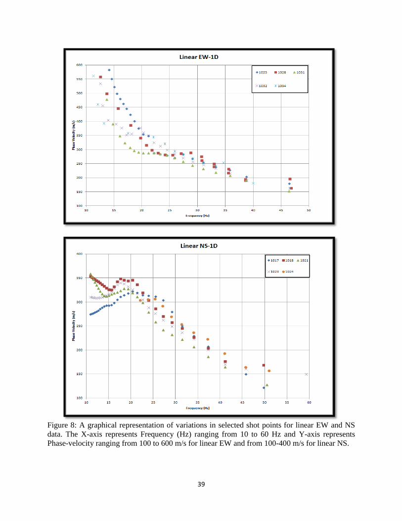
Figure 8
A graphical representation of variations in selected shot points for linear
EW and NS data. The X-axis representsFrequency (Hz) ranging from 10
to 60 Hz and Y-axis represents Phase-velocity ranging from 100 to 600
m/s for linear EW and from 100-400 m/s for linear NS.
39
Figure 9
Dispersion images for linear EW (a) and NS (b) as obtained through
stacking various shot records. The X-axis represents Frequency (Hz)
ranging from 10-100 Hz and Y-axis represents Phase-velocity (m/s)
ranging from 100-2000 m/s.
41
ix
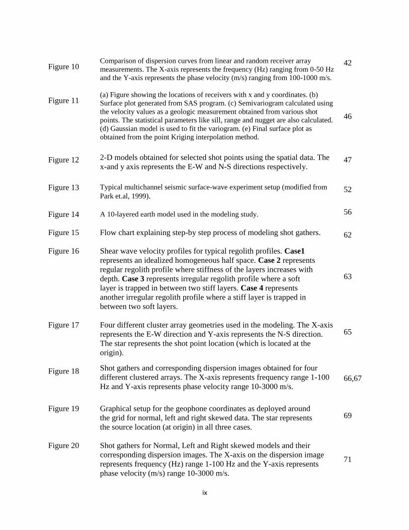
Figure 10
Comparison of dispersion curves from linear and random receiver array
measurements. The X-axis represents the frequency (Hz) ranging from 0-50 Hz
and the Y-axis represents the phase velocity (m/s) ranging from 100-1000 m/s.
42
Figure 11
(a) Figure showing the locations of receivers with x and y coordinates. (b)
Surface plot generated from SAS program. (c) Semivariogram calculated using
the velocity values as a geologic measurement obtained from various shot
points. The statistical parameters like sill, range and nugget are also calculated.
(d) Gaussian model is used to fit the variogram. (e) Final surface plot as
obtained from the point Kriging interpolation method.
46
Figure 12
2-D models obtained for selected shot points using the spatial data. The
x-and y axis represents the E-W and N-S directions respectively. 47
Figure 13 Typical multichannel seismic surface-wave experiment setup (modified from
Park et.al, 1999). 52
Figure 14 A 10-layered earth model used in the modeling study. 56
Figure 15 Flow chart explaining step-by step process of modeling shot gathers. 62
Figure 16
Shear wave velocity profiles for typical regolith profiles. Case1
represents an idealized homogeneous half space. Case 2 represents
regular regolith profile where stiffness of the layers increases with
depth. Case 3 represents irregular regolith profile where a soft
layer is trapped in between two stiff layers. Case 4 represents
another irregular regolith profile where a stiff layer is trapped in
between two soft layers.
63
Figure 17
Four different cluster array geometries used in the modeling. The X-axis
represents the E-W direction and Y-axis represents the N-S direction.
The star represents the shot point location (which is located at the
origin).
65
Figure 18 Shot gathers and corresponding dispersion images obtained for four
different clustered arrays. The X-axis represents frequency range 1-100
Hz and Y-axis represents phase velocity range 10-3000 m/s. 66,67
Figure 19 Graphical setup for the geophone coordinates as deployed around
the grid for normal, left and right skewed data. The star represents
the source location (at origin) in all three cases.
69
Figure 20
Shot gathers for Normal, Left and Right skewed models and their
corresponding dispersion images. The X-axis on the dispersion image
represents frequency (Hz) range 1-100 Hz and the Y-axis represents
phase velocity (m/s) range 10-3000 m/s.
71

x
Figure 21
Modeled shot gathers and corresponding dispersion images for different
number of channels. The X-axis represents frequency range 1-100 Hz
and Y-axis represents phase-velocity range 10-3000 m/s.
72
Figure 22
Location of the University of Tennessee Agricultural Extension Center,
Knoxville, TN. The yellow square located in the zoomed in map shows
the location of the study area (Google Earth).
77
Figure 23
The figure on the left represents the shot point locations as deployed on the
ground. There are total 13 shot points from which data was collected. The
distance between each shot point location is 10 m. The figure on the right
represents the random arrangement of geophones (small circles) inside a 10
m×10 m grid.
78
Figure 23
Schematic representation of steps involved in data processing and
analysis. 79
Figure 24 Shot gathers for various arrays. The X-axis represents offset (m) and trace
numbers and Y-axis represents time (ms). Data was collected for 1000ms
but only the first 500ms is shown here.
81
Figure 25
Schematic representation of various array designs (a) conventional arrays
(b) four different random arrays as deployed in the field. The X-axis
represents E-W and Y-axis represents the N-S directions. Each square
represents the 10 by 10 grid and 13 shot points were deployed around this
grid whose locations are shown in Figure 23.
83,84
Figure 26 Schematic representation of steps involved in data processing and
analysis. 83
Figure 27 A screenshot image of the receiver coding module that was used in 2-D
receiver array processing. 88
Figure 28
Dispersion images for (a) conventional Linear (EW and NS), Cross, and
Circular receiver arrays and (b) for four different random receiver arrays.
The X-axis represents Frequency (Hz) and Y-axis represents Phase
Velocity (m/s). Data were processed for frequencies from 1-100 Hz and
phase velocities from 100-3000m/s but data here is displayed only from
10-50 Hz as surface wave dispersion curves are dominant here.
89,90
Figure 29
A graph representing dispersion curve comparison for four types of
receiver arrays. The X-axis represents frequency (Hz) ranging from 10-
40 Hz and Y-axis represents phase-velocity (m/s) ranging from 0-1000
m/s.
91

xi
Figure 30
Comparison of dispersion curves for various random array distributions.
The X-axis represents frequency (Hz) ranging from 10-35 Hz and Y-axis
represents phase-velocity (m/s) from 0-1000 m/s. It is observed that
random 1,2, and 3 curves show higher velocity values when compared to
random 4.
91
Figure 31
Schematic graphs representing dispersion picks split up into 10-20 Hz and
15-40 Hz to observe the differences within the dispersion picks for clarity.
It can be observed that at lower frequencies the phase velocity values agree
closely with each other and at higher frequencies (starting from 18 Hz to 32
Hz) the random deviates from the conventional arrays.
92
Figure 32
Dispersion images for selected shot records from linear EW data. The
image on the left was processed using the traditional MASW processing
scheme and the image on the right was processed using the XY coding
module. The X-axis represents Frequency (Hz) and Y-axis represents
Phase-velocity (m/s).
94
Figure 33 Graphs representing the variations in the shear-wave velocity values as
obtained from inverting the dispersion picks of above shown dispersion
images. The blue dots represent the Vs values from traditional processing
scheme and the red dots represent the ones obtained from the 2-D
processing scheme.
95
Figure 34 Graphical representation of variations in dispersion curves for various
receiver arrays with the two types of processing schemes. The X-axis
represents Frequency (Hz) and Y-axis represents Phase-velocity (m/s).
96
Figure 35 (a) 1-D shear wave velocity profiles for various conventional and random
receiver arrays obtained by inverting the phase velocity picks from Figure 28
(a). (b) 1-D shear wave velocity profiles for various random arrays obtained by
inverting the phase velocity picks from figure 28 (b).
100
Figure 36 Graphical comparison of different conventional and random array 1-D
Vs profiles. Random 4 data was used here as it gave the closest dispersion
curve values to the conventional data.
109
Figure 37 Graphical comparison of four different random array 1-D Vs profiles. 101
Figure 38
Schematic stratigraphic column representing various regolith layers with
approximate depths (in meters) as obtained from the bedrock core- hole
log data obtained by Hydrogeology division, University of Tennessee-
Knoxville (Benfield et al., 2003).
102
Figure 39 Interaction plot for Vs with depth for different geophone arrays. 105

xii
Figure 40
(a) Sunset crater and the Black Point Lava Flow (BPLF), north of
Flagstaff, AZ. (b) Box marks the far-east side of the BPLF where seismic
data was collected. (Google Earth) (c) A snapshot of the field site.
112
Figure 41 (a) The figure represents the shot point locations as deployed on the
ground. There are a total of nine shot points for the 2-D arrays. The
yellow markers represent the shot point locations. (b) Schematic
representation of various receiver arrays as deployed in the field. X- axis
represents E-W traverse and Y-axis represents N-S traverse (i) Linear
EW (ii) Linear NS (iii) Cross (iv) Random.
113
Figure 42
Typical shot gathers for various array types as acquired from the BPLF field
site. Data was collected for 1000 ms but only the first 500 ms data is shown
here as surface waves are more prominent here.
115
Figure 43
Dispersion images obtained from shot gathers for various receiver arrays in
Figure 34. The X-axis represents the frequency (Hz) and Y-axis represents the
phase velocity (m/s). The white dots on the dispersion image represent the
fundamental mode picks for various receiver arrays.
118
Figure 44 The 1-D shear wave velocity profiles obtained from the dispersion curves
extracted from the dispersion images in Figure 4. The X-axis represents the
shear wave velocity (m/s) and the Y-axis represents the depth (m).
119
Figure 45
A graph comparing dispersion curves for various receiver arrays. The X-axis
represents frequency (Hz) and Y-axis represents phase velocity (m/s).
120
Figure 46
Velocity (m/s) versus depth (m) a comparison for various receiver
arrays. The X-axis represents shear wave velocity (m/s) and Y-axis
represents depth (m).
121
Figure 47
Least-square means for depth as calculated from mixed model analysis
for the inversion data.
125
Figure 48
Graphical representation of Vs profiles for all receiver array types shown
together in a single graph.
127
Figure 49
Interpreted regolith profile as estimated for the conventional linear array and
newly developed random array for up to 20 m depth.
128

1
CHAPTER-1
Introduction
2
1.1 MOTIVATION
Subsurface imaging is very critical not only for exploring underground resources but also to
determine important geotechnical parameters like the shear wave velocity, shear modulus, etc.
for the upper 30 m of subsurface. Understanding the behavior of regoliths to various types of
loading conditions is a primary goal in geotechnical engineering. Engineering properties, like the
shear modulus and Poisson’s ratio, are critical parameters with respect to most civil engineering
works as they characterize the mechanical behavior of geotechnical materials under various types
of loading. Therefore, the in situ estimation of shear wave velocity of regoliths is critically
important in terms of determining the shear modulus of regolith, regolith, and rock. Although
there exist some conventional principle methods to obtain such information, like drilling
boreholes, seismic cone penetrometer tests (SCPT) etc. these methods are all impractical,
imprudent and impossible to deploy under certain field conditions where it is inaccessible and/or
restricted. Therefore scientists have developed a new technique, the seismic method. One such
seismic method that has gained popularity in recent years is the multi-channel analysis of surface
wave (MASW) method. The MASW method involves deployment of multiple seismometers to
acquire 1-D or 2-D shear wave velocity profiles that can be directly related to various
engineering properties. The advantage of this technique over drilling boreholes, cone
penetrometers or any other geophysical technique is that it is less intensive, non-invasive, more
cost-effective, and more robust because strong surface-wave records are almost guaranteed. In
addition, data processing and analysis is fairly straightforward, and the MASW method allows
for analysis of a large area of interest as compared to drilling boreholes. A new scheme using
randomly distributed geophones (likely deployed from a mortar-type device) instead of a
conventional linear array will be presented in this study. Such type of arrangement will be

3
necessary in places that are inaccessible such as battle fields, urban settings, and even on any
kind of off-earth objects because of the logistical constraints involved in deploying a linear or
circular array robotically or by astronaut. Therefore the main hypotheses for this study is that the
random array MASW will provide information about the engineering properties of the upper 30
m of the subsurface while being deployable under any type of logistical conditions and also that
the MASW method when used with random geophone array can be used to determine
geotechnical properties under different geologic settings.
1.2 RESEARCH OBJECTIVES
The main focus of research in this study is to improve and increase the usage of MASW
method in determining regolith and rock properties by introducing a new type of receiver
arrangement to extend its usage in places that are inaccessible such as in battle fields, urban
settings and even on other planetary bodies like the Moon, Mars, or other solid bodies in the
solar system. Both field tests and numerical simulations are used to examine this issue. The
successful application of the results obtained from this study will help not only the geotechnical
community but also other scientific communities by obtaining more reliable determination of
regolith properties and readily-deployable data techniques.
The first objective of this research is to investigate a new method suitable and applicable not
only on the earth but also on other off-earth objects such as the Moon, Mars, Near Earth
Asteroids (NEA’s) etc., to estimate geotechnical properties. Geotechnical or engineering
properties are those properties that effect construction and engineering. Engineering properties--
like shear strength, shear modulus and Poisson’s ratio--are key parameters for civil engineering
works, as they characterize the mechanical behavior of geotechnical materials under various

4
types of loading. The multi-channel seismic method has previously been demonstrated to greatly
increase our ability to map shear-wave velocities and subsurface variations in physical
properties. However, considering the logistical constraints involved in deploying linear or
circular array robotically or by astronaut, a random array will be better suited for places that are
inaccessible. Therefore, the first hypothesis of this research is that a random-array seismometer
deployment scheme can be used to obtain reliable and high resolution dispersion images.
The second objective of this research is to acquire MASW data for various conventional
geophone arrays—such as the linear, cross, and circular—as well as a random deployment for
direct comparison. The main hypothesis is that conventional and newly developed arrays will
yield similar results, as demonstrated by a correlation between the dispersion curves and the
accuracy of the shear-wave velocity profiles. As a follow on component of this objective,
computer simulations are conducted to study various effects such as increasing grid size,
increasing numbers of receiver, etc. Simulation models are generated for various possibilities of
rock/regolith property variations under certain parameters like varying velocities, frequencies,
and depth to the subsurface.
The third objective is a field-based approach used to apply the results from objectives one &
two by determining engineering properties for the upper 30 m on terrestrial analog environments,
such as the Black Point Lava Flow (BPLF) to help predict the nature of subsurface that can be
encountered during future landed scientific or engineering operations on any kind of planetary
surface. A previously-determined terrestrial analog site with a completely different geologic
setting than the controlled site was selected, and near-surface seismic data has been acquired
using random arrangement of geophones. The hypothesis of this objective is that the random-
array MASW technique can yield acceptable results on terrestrial analog environments.

5
1.3 DISSERTATION OUTLINE
Following this introduction in Chapter 1, Chapter 2 is used to briefly describe the behavior of
Rayleigh waves in homogeneous and heterogeneous media followed by a brief overview of
MASW method. This will lay the fundamental groundwork for subsequent chapters.
Chapter 3 presents the newly-developed random receiver array technique, including the data
acquisition and processing scheme. Preliminary results obtained from this technique are also
presented. These results are briefly compared with conventional linear geophone array in order
to show the correlation between them and set the stage for the next chapters.
Chapter 4 presents results of a suite of numerical simulations that are performed to study the
effect of various parameters pertaining to random array geometry such as clustering effects,
skewness effects, and total number of seismometers used within the random geophone array.
Comparison of field and modeled data results are presented.
Chapter 5 presents a detailed comparison study between the traditional geophone arrays like
the linear, cross, & circular with that of the newly developed random-geometry geophone array.
This is mainly used to examine and identify the effectiveness/advantages from the use of random
geophone array with respect to data acquisition, dispersion imaging, azimuthal variations etc.
Chapter 6 covers the applicability of random array MASW method to delineate geotechnical
properties of subsurface in a field-based case study. The results obtained from the Black Point
Lava Flow (BPLF) site-a terrestrial analog environment are presented, including elucidation of
the significance of the chosen site as compared to other prominent locations.

6
Finally, Chapter 7 provides the summary and conclusions of this research and
recommendations for future work.
1.4 SIGNIFICANCE OF THE STUDY
A novel technique of using a random arrangement of geophones instead of conventional
arrays will be introduced from this study. Such arrangement will be critical in hard-to-reach
places including battle fields, urbanized areas, and even on other planetary surfaces such as
moon, mars etc. as space exploration advances and long-term human habitation becomes
necessary. Although conventional array types have proven adept for delineating regolith
properties, the type of array that you choose is at least partially controlled by the site viability
and other conditions. Thus, in some cases where there might be places that can be
unreachable or it is simply not possible to arrange a systematic linear or circular array
robotically (or by an astronaut) on the surface due to logistical reasons, a randomly
distributed geophone array (likely to be deployed using a mortar-type device) will be most
useful. Additionally there is information that can be obtained from random array like the
azimuthal variations in the subsurface that are likewise difficult to determine using other
geophone arrangements.

7
CHAPTER 2
Overview of surface wave theory
8
2.1 INTRODUCTION
Surface waves were first introduced by Lord Rayleigh as the solution of the equation of
waves propagating along the free surface of an elastic half-space in 1885 (Rayleigh, 1885). In
geotechnical engineering, surface waves have been used to determine the dynamic properties of
near-surface regolith, regolith, and bedrock non-invasively for the past 50 years (e.g., Jones, 1958;
Richard et al., 1970; Nazarian, 1984; Stokoe et al., 1994; Tokimatsu, 1995; Rix et al., 2001b;
Okada, 2003). Surface wave methods are based on measured vertical particle motions of Rayleigh
waves at various locations on the ground surface. The measured motions depend on the properties
of the medium, the frequency of the waves, and the distance from a source location to the ground-
motion detectors (seismometers or geophones).
In this chapter, the theoretical study of Rayleigh wave propagation in homogeneous and
layered media is addressed. A layered medium consisting of a stack of homogeneous, isotropic,
and elastic layers overlying a homogeneous half-space represents an appropriate model for
vertically heterogeneous regolith/rock profiles. The layered model is often used in inversion
procedures of surface wave methods due to computational efficiency.
2.2 RAYLEIGH WAVES IN LAYERED MEDIA
2.2.1 Dispersion equation
In the real world, assuming a homogenous half space for modeling subsurface properties
is a bit too simple and unrealistic. Instead, subsurface properties that vary with depth may be
idealized using a simplified layered model as shown in Figure 1. This simplification consists of
N number of homogenous, isotropic, elastic layers characterized with properties like shear wave
velocity (Vs), density (ρ), Poisson’s ratio (Φ) and thickness (h). These types of layered media are

9
modeled frequently in most geotechnical cases due to computational efficiency, and yield robust
approximations.
The boundary conditions that are applied for a homogenous half space are (i) no stress at
the surface and (ii) zero amplitude at infinite depth. These conditions are also typically valid for
the layered media with extra boundary conditions applied to the continuity in stress and
displacements at the interface between each layer, and these additional boundary conditions are
expressed as:
where n=1,……,N
Displacements un (x, z) in each layer are obtained by:
Application of the boundary conditions in equations 2.31 and 2.32 will yield a homogeneous
system of 4N-2 linear equations, denoted by S. Non-trivial solutions can be obtained by setting
det[S]=0, and this leads to the final product that is called the Rayleigh dispersion equation for a
layered half-space. The equation provides an implicit relationship between the phase velocity of
Rayleigh waves, frequency, and the properties of the layers, and can be written (Lai, 1998):
(2.29)
(2.30)
(2.31)
(2.32)

10
It is evident from equation 2.33 that the phase velocity of Rayleigh waves in a vertically
heterogeneous medium is dependent on frequency. This phenomenon is known as geometric
dispersion, since it is related to the geometrical variations of properties with depth. Therefore, it
is the key element in surface wave methods that Rayleigh waves with different wavelengths
(frequencies) sample different parts of layered medium (see Stokoe et al., 1994) allowing them to
be used to determine variations in material properties with depth. However, for a given
frequency, there exist multiple solutions for the Rayleigh dispersion equation. This means that
for a given frequency, multiple modes for a given frequency traveling at different phase
velocities exist. The concept of multiple modes can be explained physically by the constructive
interference occurring among waves undergoing multiple reflections at the layer interfaces (see
Lai, 1998).
(2.33)

11
Figure 1. Vertical particle motions of two Rayleigh waves with different wavelengths (modified
from Rix, 2000)
2.2.2 Phase velocities of Rayleigh waves
In most cases, differential eigenvalue problem (e.g., Aki and Richards, 1980) is used as
an alternative formulation of the Rayleigh wave dispersion equation. A linear differential
eigenvalue problem with displacement eigenfunctions r1(z,k,ω) and r2(z,k,ω) and stress
eigenfunctions r3(z,k,ω) and r4(z,k,ω) in a layered medium is defined by:
(2.34)
12
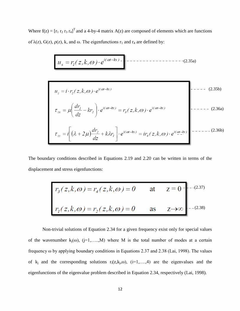
Where f(z) = [r1 r2 r3 r4]T
and a 4-by-4 matrix A(z) are composed of elements which are functions
of λ(z), G(z), ρ(z), k, and ω. The eigenfunctions r1 and r4 are defined by:
The boundary conditions described in Equations 2.19 and 2.20 can be written in terms of the
displacement and stress eigenfunctions:
Non-trivial solutions of Equation 2.34 for a given frequency exist only for special values
of the wavenumber kj(ω), (j=1,…..,M) where M is the total number of modes at a certain
frequency ω by applying boundary conditions in Equations 2.37 and 2.38 (Lai, 1998). The values
of kj and the corresponding solutions ri(z,kj,ω), (i=1,….,4) are the eigenvalues and the
eigenfunctions of the eigenvalue problem described in Equation 2.34, respectively (Lai, 1998).
(2.35a)
(2.35b)
(2.36a)
(2.36b)
(2.37)
(2.38)

13
The values of kj for Rayleigh waves in the layered medium can be obtained by solving the
Rayleigh dispersion equation in Equation 2.33 using solution techniques like transfer matrix
method (Thomson 1950; Haskell 1953; Schwab and Knopoff, 1970; Abo-Zena, 1979), stiffness
matrix method (Kausel and Roesset, 1981), and reflection and transmission coefficients method
(Kennett, 1974; Kennett and Kerry, 1979; Luco and Aspel, 1983; Hisada, 1994; Hisada, 1995).
Once the roots of the Rayleigh dispersion equation, i.e., the values of kj, are obtained using one
of the above solution methods, the eigenfunctions ri(z,kj,ω) satisfying Equation 2.34 can be
easily calculated. Each pair of ri(z,kj,ω) and kj defines a specific mode of Rayleigh wave
propagation. On the other hand, in a medium consisting of a finite number of homogeneous
layers overlying a homogeneous half-space, the total number of modes of Rayleigh wave
propagation is always finite (Ewing et al., 1957).
2.3 SURFACE WAVE THEORY
As described above, there are two types of surface waves: Rayleigh and Love waves
(Dobrin and Savit, 1988). Both represent the plane-wave solutions to the coupled elastic wave
equation (see Haskell, 1953):
∂2/∂t
2 = Vp
2
2 and ∂
2/∂t
2 = Vs
2
2……(3.1)
In most of near-surface active-source seismic surveys when a compressional source is used, more
than two-thirds of total seismic energy generated is imparted into Rayleigh waves (Richart et al.,
1970), which is the principal component of surface waves generated most effectively in all kinds
of surface seismic surveys. As previously described, surface waves obey the property of
dispersion i.e. for a vertical velocity variation, each frequency component of a surface wave has
a different propagation velocity (also called phase velocity), that in turn results in a different
wavelength for each frequency of the propagated wave. Therefore, due to its dispersive property,

14
ground roll can be utilized to infer near-surface elastic properties (Nazarian et al., 1983; Stokoe
et al., 1994; Park et al., 1998a).
Constructing shear-wave velocity profiles through the analysis of plane-wave
fundamental mode Rayeligh waves is one of the most common ways to use the dispersive
properties of surface waves (Bullen, 1963). The phase velocities for different wavelengths can be
found from the solutions to the wave equation (as described in Chapter 2) by treating the near
surface materials as layered earth medium (Haskell, 1953). Therefore, by analyzing the
dispersion feature of ground roll represented in recorded seismic data, the near-surface S-wave
velocity (Vs) profiles can be constructed and the corresponding shear moduli () are calculated
from the relation between the two parameters.
Vs =(/)1/2
…..(3.2)
where represents the density of material (assumed as constant since it varies little with depth
(as compared to the scale of variations in bulk and shear modulus).
2.4 OVERALL MASW PROCEDURE
The MASW method utilizes multi-channel recording and processing concepts widely
used in near-surface seismology as well as in reflection surveying for oil exploration. The
fundamental mode the Rayleigh is without a doubt one of the most troublesome types of source-
generated noise on reflection surveys. Rayleigh-wave energy is defined as signal in MASW
analysis, and needs to be enhanced during both data acquisition and processing steps. In all kinds
of surface seismic surveys using vertical sources, ground roll takes more than two thirds of total
generated seismic energy and usually appears with the most prominence on the Multi-channel

15
records. Therefore, generation of ground roll is easiest among all other types of seismic waves.
The field setup is shown schematically in Figure 2. The method first requires measurement of
seismic surface waves generated from various types of seismic sources—such as sledge
hammer—and the propagation velocities of those surface waves is analyzed, and finally the
shear-wave velocity (Vs) variations below the surveyed area that is most responsible for the
analyzed propagation velocity pattern of surface waves is calculated.
The most common procedure that is followed for typical MASW surveys include three major
steps:
1. Data acquisition: acquiring multichannel field records
2. Dispersion analysis: extracting dispersion curves
3. Inversion: Inverting to yield shear-wave velocity variation with depth
Subsequently, a 2-D cross-sectional Vs map may be constructed through an appropriate
interpolation scheme by placing each 1-D Vs profile at surface location corresponding to the
middle of the receiver line. Detailed step by step procedure for each of the step is explained
below and the optimum field parameters are also tabulated.
2.4.1 Field procedure: Data acquisition
This subsection is used to describe the entire field procedure for MASW data acquisition.
Among the active and passive MASW, the active method is the most common type for acquiring
2-D Vs profiles. The maximum depth of investigation (Zmax) that can be achieved from the
survey is usually 10-30 m range and varies with the type of source used. Some of the parameters
related to data acquisition procedure are described below. Table 1 describes the optimum field

16
parameters for a typical data acquisition procedure, keeping in mind the fact that these can be
changed or updated by investigators and practitioners depending upon the requirements and in-
field conditions.
Figure 2. Schematic representation of the active MASW field survey (modified from Park, 2003)
Source
Maximum investigation depth (Zmax) is determined by the longest wavelength (Lmax) of
the surface waves used for the analysis as Zmax=0.5Lmax. Also, Lmax is governed by the energy
and area of impact of the seismic source, which may be controlled type (like the sledge hammer
in case of an active survey) or passive (via a car moving or other kinds of cultural noise).
According to the above relation, the longer Lmax, (deeper the Zmax) can be achieved with a
greater impact power. Some of the commonly used sources include a heavy sledge hammer (10-
20 lb), weight-drop etc. Using an impact plate (also called base plate) will help the source impact
point intrude less into regolith. The table below explains different optimum sources for different
investigation depth. For unusually shallow investigation, a relatively light source has to be used
17
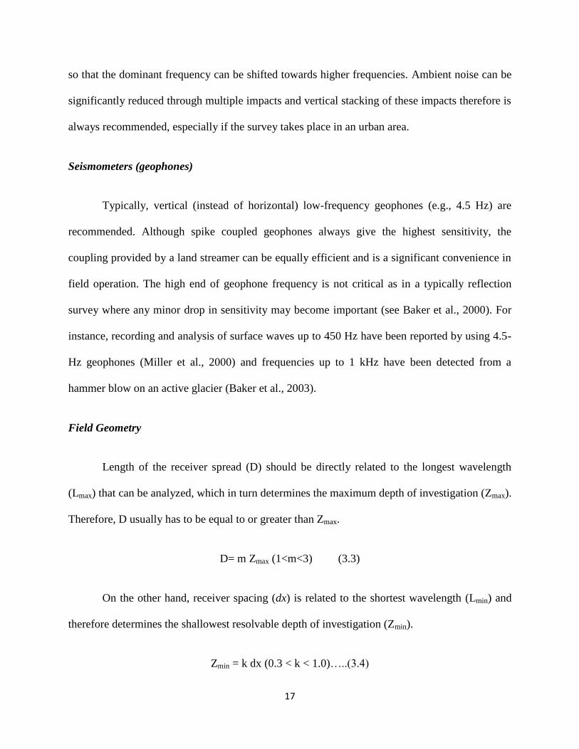
so that the dominant frequency can be shifted towards higher frequencies. Ambient noise can be
significantly reduced through multiple impacts and vertical stacking of these impacts therefore is
always recommended, especially if the survey takes place in an urban area.
Seismometers (geophones)
Typically, vertical (instead of horizontal) low-frequency geophones (e.g., 4.5 Hz) are
recommended. Although spike coupled geophones always give the highest sensitivity, the
coupling provided by a land streamer can be equally efficient and is a significant convenience in
field operation. The high end of geophone frequency is not critical as in a typically reflection
survey where any minor drop in sensitivity may become important (see Baker et al., 2000). For
instance, recording and analysis of surface waves up to 450 Hz have been reported by using 4.5-
Hz geophones (Miller et al., 2000) and frequencies up to 1 kHz have been detected from a
hammer blow on an active glacier (Baker et al., 2003).
Field Geometry
Length of the receiver spread (D) should be directly related to the longest wavelength
(Lmax) that can be analyzed, which in turn determines the maximum depth of investigation (Zmax).
Therefore, D usually has to be equal to or greater than Zmax.
D= m Zmax (1<m<3) (3.3)
On the other hand, receiver spacing (dx) is related to the shortest wavelength (Lmin) and
therefore determines the shallowest resolvable depth of investigation (Zmin).
Zmin = k dx (0.3 < k < 1.0)…..(3.4)
18
The source offset distance (x1) is also a major governing factor to predict the degree of
contamination by the near-field effects that indicate a confluence of all adverse influences on
data acquisition, mainly because of the source being too close to the geophones resulting in
“clipping” of the digital record. Although its optimum value is still under debate, a value of 20%
of D is suggested as a minimum and 100% as a maximum. A larger value of x1 and D will
increase the risk of higher-mode domination and reduce S/N for the fundamental mode.
Occasionally while performing an active linear survey where the total profile length is
significantly longer than the available geophone spread, sometimes a roll-along spread is used.
In that case, the interval (dSRC) of source-receivers configuration move between 1dx-12dx is
recommended for 24-channel acquisition. This particular variable is also directly related to the
horizontal resolution. Obviously, as the number of available channels increases, the ability to
acquire data along a profile without a roll-along spread is increased.

19
Table 1. Data acquisition parameters for active survey. Recommended values in ( )
Recording Parameters
A one-millisecond of sampling interval (dt=1 ms) is most commonly used with a 1-sec
total recording time (T=1 sec). A smaller dt is recommended if any body-wave processing is
planned as by product and a longer T is recommended in case of extremely low velocities or if a
longer receiver spread (D) is used. An excessively longer T, when used, may increase the chance
of recording ambient noise. Generally, shorter dx and longer D combination is recommended.
When more channels are used the Signal-to-noise ratio (S/N) will be increased during data
analysis because of the redundancy as well as the possibility of increasing resolution at shallow
depths. Also the effect of increasing D will be an increased Zmax.
Depth (Zmax) (ft)
Source (S) (lb)
Receiver(R) (Hz)
Receiver Spread (RS) (ft)
Length (D) Source offset (X1)
Receiver spacing (dx)
24-ch 48-ch
SR Move (dx)
Lateral Resolution
High Medium Low
Recording
dt (ms) T(sec)
Vertical Stack
C N VN
≤ 5.0
5-15
15-30
30-60
60-100
100-150
>150
≤ 1(1)
1-5(5)
5-10(10)
>10(20)
>10(20)
>10 (20)(passive)
>10 (20)(passive)
4.5-100(40)
4.5-40(10)
≤ 10(4.5)
≤ 10(4.5)
≤ 4.5(4.5)
≤ 4.5(4.5)
≤ 4.5(4.5)
5-15(10)
5-45(30)
15-90(50)
30-180(120)
60-300(200)
100-450(300)
>150(450)
1-15(2)
1-9(5)
3-18(10)
6-36(30)
12-60(40)
20-90(60)
>30(100)
0.2-0.6(0.3)
0.2-2.0(1.0)
0.5-4.0(2.0)
1.0-8.0(4.0)
2-12(8)
4-18(12)
>6.0(20)
0.1-0.3(0.2)
0.1-1.0(0.5)
0.2-2.0(1.0)
0.5-4.0(2.0)
1-6(4)
2-9(6)
>3.0(10)
1-2(1)
1-2(1)
1-2(1)
1-2(1)
1-2(1)
1-2(1)
1-2(1)
2-4(2)
2-4(2)
2-4(2)
2-4(2)
2-4(2)
2-4(2)
2-4(2)
4-12(4)
4-12(4)
4-12(4)
4-12(4)
4-12(4)
4-12(4)
4-12(4)
0.5-1.0(0.5)
0.5-1.0(0.5)
0.5-1.0(0.5)
0.5-1.0(0.5)
0.5-1.0(0.5)
0.5-1.0(0.5)
0.5-1.0(0.5)
0.5-1.0(0.5)
0.5-1.0(0.5)
0.5-1.0(1)
1.0-2.0(1)
1.0-2.0(1)
1.0-3.0(1)
>1.0(2.0)
1-3(3)
1-3(3)
1-3(3)
1-3(3)
1-3(3)
1-3(3)
1-3(3)
3-5(5)
3-5(5)
3-5(5)
3-5(5)
3-5(5)
3-5(5)
3-5(5)
5-10(10)
5-10(10)
5-10(10)
5-10(10)
5-10(10)
5-10(10)
5-10(10)
*** SR Move represents distance in receiver spacing (dx) that the source (S) and Receiver (R) setup moves after
acquiring data at one location; dt represents sampling interval in milliseconds (ms); T represents total recording
time in seconds (sec); Vertical stack is the number of stacking data in seismograph’s memory before being saved
under different conditions of calm (C), noisy (N), and very noisy (VN) environment, respectively. These
parameters given here are just a list of optimum parameters and are by no means definitive or required. There is a
tolerance level of +/- 20% to most of these recommended values.
20
2.4.2 Field procedure: Data Analysis
The first step in data analysis involves extracting dispersion curves from the data that are
in turn used in the subsequent step of data inversion, whereby a proper layer (shear-wave
velocity-Vs) model is determined such that the theoretical dispersion curves match the measured
ones as close as possible. Usually, the fundamental mode (M0) curve is used. However, recent
studies (Xia et.al., 2000a) suggest that higher-modes can also be utilized to get shear-wave
velocity information.
Concept of Dispersion
In the early stage of surface wave method using monotonic vibrator exciting at a single
frequency (f) at a time, the distance (Lf) between two consecutive amplitude maxima was
measured by scanning the ground surface with a single sensor and an oscilloscope. Then,
corresponding phase velocity (Cf) was calculated as Cf=Lf*f. This measurement was then
repeated for different frequencies to construct a dispersion curve with the assumption that the
fundamental mode (M0) of the surface wave dominate in the field. In early 1900’s this method
was used efficiently by the spectral analysis of surface waves (SASW) method. Instead of trying
to measure the distance of Lf, the method is used to measure the phase difference (dp) for a
frequency (f) between the two receivers a known distance apart from the relationship:
Cf=2*pi*f/dp. This process is repeated for different frequencies to construct a dispersion curve.
The possibility of multi-modal influence during the inversion process is accounted for with the
concept of apparent dispersion curve.
While using a multi-channel approach, however, the user does not calculate individual
phase velocities first, but instead construct an image space whereby dispersion trends are

21
identified from the pattern of energy accumulation (higher amplitude peaks) in this the
frequency-wave number domain. Then, necessary dispersion curves are extracted by following
the image trends based on the amplitude anomalies. During this imaging process, a multichannel
record in time-space domain is transformed into either frequency-wave number or frequency-
phase velocity domain. In order to acquire this, the phase-shift method is generally used instead
of any other traditional method like pi-omega or the f-k method because it achieves higher
resolution than the other methods (from www.masw.com).
The Dispersion imaging scheme
The standard data processing scheme is as follows: A multi channel field record (a) is
first decomposed via Fast Fourier Transformation (FFT) into individual frequency components,
and then amplitude normalization is applied to the each component (b). Then, for a given testing
phase velocity in a certain range, necessary amount of phase shifts are calculated to compensate
for the time delay corresponding to a specific offset, applied to individual component, and all of
them are summed together to make a summed energy of (c). This in turn is repeated for different
frequency components. When all the energy is summed in frequency-phase velocity space, it will
show a pattern of energy accumulation that represents the dispersion curve as shown in (d). In
case of multi-modal dispersion, that behavior of energy will appear as multiple energy
accumulations for a given frequency as shown in (e).
2.4.3 Field Procedure: Data Inversion
Inversion in general
Inversion or inversion modeling, in general, attempts to seek the cause to a result when
the result is known. On the other hand, predicting the result from the given cause is referred to as

22
forward modeling. An inversion is known to be unique if there is only one solution to the
problem, and non-unique if multiple solutions exist. It is also called “linear” if the cause-related
relationship is linear as a small change in input yields also a small change in result, whereas
“non-unique” if a small change can give rise to a big change in result.
Typical MASW method inversion
The goal of a field survey and data processing in MASW is to establish the fundamental
mode (M0) dispersion curve as accurately as possible. Theoretical M0 curves are then calculated
for different earth models by using a proper forward modeling scheme (e.g., Schwab and
Knopoff, 1972) to be compared against the measured curve. The process of inversion is based on
the assumption that the measured dispersion curve represents the M0 curve only, not influenced
by any other modes of surface waves. The most important issue with the inversion process is to
determine the best-fit earth model among many different models as efficiently as possible. One
way to check for the closeness between the measured and theoretical curves is the root-mean
square (RMS) error factor. Several other types of inversion are described below.
Multi-modal Inversion
The multi-modal inversion technique utilizes both the fundamental and higher-mode
curves for the inversion. This is done in order to increase the accuracy (resolution) of the final 1-
D Vs profile by narrowing the range of solutions with 1-D Vs profiles otherwise equally well
suited if only the M0 curve is used. This method can also be used to alleviate the inherent
problem with the inversion method of non-uniqueness in general.

23
Dispersion Image Inversion
The method of inversion includes the use of dispersion image data (also called phase-
velocity spectra) instead of dispersion curves, and does not involve the extraction of modal
curves at all (Ryden and Park, 2006; Forbriger, 2003a;2003b). This approach eliminates such
drawbacks with the modal-curve based inversion such as mode-misidentification and mode-mix
problems (misidentifying higher mode curve as a M0 curve) if data acquisition and subsequent
processing are not properly performed. Dispersion curves when misidentified may lead to
erroneous Vs profile because of the lack of compatibility in the inversion process trying to match
measured and theoretical curves.
Raw Data Inversion
As the name suggests, this type of inversion utilizes the raw multichannel record instead
of the one processed for dispersion imaging (Forbriger, 2003b). In the process, the scheme
attempts to compare whole seismic waveforms observed at different distances from the source
with synthetic waveforms generated from a forward modeling scheme. This type of approach
may be advantageous over others for the fact that it is not biased by any other kind of data
processing such as dispersion imaging or curve extraction. At the same time, however, it has to
take into account the attenuation and interference issues, as well as layer parameters, since all of
these can contribute to the shaping of a seismic waveform.
2-D Vs Inversion
This approach uses the final output of 2-D Vs profile from current typical inversion
approach as input to the second phase of the inversion based on a different forward modeling
scheme than previously used. The main objective of this method is to consider the smearing
24
effect caused by the lateral variations during dispersion analysis as much as possible by adopting
another scheme accounting for the local variation of Vs. For this purpose, the Vs structure is
provided by the previous output of the 2-D Vs profile as an initial starting model to account for
the local variations observed within an individual field record to update a certain part of the 2D
Vs model. This initial starting model most likely corresponds to the surface location of the
receiver spread used during data acquisition. Iterations can be performed for a better result. The
main drawback for this method, however, is that it is very computationally intensive.
2.5 SUMMARY
The multi-channel analysis of surface waves (MASW) method is a relatively recently
developed seismic method dealing with relatively lower frequencies and shallow investigation
depth ranges than any other many other conventional seismic methods. The data acquisition and
processing scheme results (Vs information) have proven to be highly reliable in geotechnical
field, even under the presence of higher modes of surface waves and also under various types of
cultural noise. The data processing steps are all automated which makes this method extremely
easy and fast to implement and also very cost-effective. Due to these advantages, this method has
gained significant importance in geotechnical engineering and also in other engineering
communities.

25
CHAPTER-3
Exploring Multi-Channel Analysis of Seismic Surface Waves with Random Receiver
Arrays for Planetary Exploration
Note: This Chapter is written specifically to be submitted directly as a manuscript.
Therefore, there is some repeated material and overlap with previous and subsequent
chapters.
Yeluru, P.M., Baker, G.S., Park, C., and Perfect, E., in prep.

26
ABSTRACT
Understanding the physical and engineering properties within the upper 30 meters of any non-
Earth object in our solar system (Moon, Mars, asteroids, etc.) will be critical as exploration
advances with deployment of large structures, as well as excavating for mining or human
habitation becomes necessary. Advances in multi-channel seismic acquisition, either active or
passive, in acquiring reliable 1-D or 2-D shear wave velocity profiles have greatly improved our
ability to determine the engineering properties (e.g., Poisson’s ratio) of Earth’s shallow
subsurface, especially when using the seismic multi-channel analysis of surface waves (MASW)
technique. The main focus of this research is to improve and increase the usability of the multi-
channel analysis of surface waves method (MASW) method in determining regolith and rock
properties by introducing a new type of receiver arrangement to extend its usage to non-Earth
environments, where engineering properties are critical but substantial logistical challenges
associated with arranging an accurate linear or circular array exist. Results indicate that robust
dispersion curves and thus subsurface models of engineering properties can be obtained using
random array geometry. This study focuses on testing the effectiveness of a random receiver
array judged by the accuracy of the dispersion curve processed from the random-array data. For
the purpose of comparison, the effectiveness of the dispersion curves obtained from the newly
developed random-array method will be compared with the conventional linear array data that is
collected at the same site. Geostatistical tools will also be used to study the data and in order to
further quantify the test (random) data obtained from different shot points.
Introduction
The shear wave velocities of near surface materials (such as regolith) are of fundamental
interest on Earth in many environmental and engineering studies and in construction safety (e.g.,
27
Park et al., 1999). For example, the average shear-wave velocity of the upper 30 m of the
subsurface (V30) plays a key role in regolith classification and is one of the critical parameters in
the construction industry and earthquake safety (Xia et al., 2007). The V30 parameter is also a
critical parameter in slope-stability analysis. Understanding the physical properties within the
upper 30 m of subsurface is important for determining rock and regolith properties that will in
turn be critical when building large structures, landing large crafts, mining for resources, and
tunneling for human habitation in case of off-earth objects. A prior knowledge of the load-
bearing capacities and structural integrity of the surface layers therefore will become important
as science advances human exploration of the solar system.
The multichannel analysis of surface waves (MASW) seismic method (e.g., Park et al.,
1999) utilizes a multi-channel seismic recording system to estimate near-surface S-wave velocity
from dispersion property of high-frequency (>2 Hz) Rayleigh waves. The method has been
steadily gaining popularity and attention from the near-surface geophysical and engineering
communities, and has been successfully applied to various near-surface problems, such as
mapping bedrock (Miller et al., 1999), studying pavement structures (e.g., Ryden et al., 2006)
and liquefaction studies (e.g., Nazarian et al., 1983). The MASW uses a multi-channel array that
makes it possible to distinguish the fundamental-mode from higher modes and body waves.
A new scheme of using randomly distributed geophones that would be deployed from a
mortar-type device instead of a conventional linear array is necessary for future space
exploration because of the substantial logistical challenges associated with arranging an accurate
linear or circular array robotically over rubberized terrain. For example, rovers that are used to
move around on planetary surfaces cannot easily move in a linear fashion or in a symmetrical
circular motion to arrange the geophones due to constraints imposed by surface clutter such as

28
rocks and boulders. The principle objective of this study, therefore, is is to assess our ability to
obtain accurate dispersion properties that can help determine engineering properties for the upper
30 m of the subsurface by using the 1-D shear wave profiles obtained using random array of
geophone placement.
3.2 OVERVIEW OF MASW METHOD
In order to acquire typical MASW data, multiple receivers (usually 24 or more) are deployed
with even spacing along a linear array with all the receivers connected to a single recording
device (seismograph) (Figure 3(a)). Each channel is dedicated to recording vibrations from one
receiver. Each multi channel record, also known as a shot gather, consists of multiple number of
time series (called traces) from all the receivers in an ordered manner. The recorded shot gather
can have various patterns depending on the type of receiver array used. A typical shot gather for
a linear array is shown in Figure 3(a).

29
Figure 3. (a) Typical multichannel seismic surface-wave experiment setup and (b) MASW data
processing procedure (modified from Park et al., 1999)
The data processing usually consists of three steps (Figure 3 b): the first step involves
converting the acquired SEG-2 format data into KGS format, and then sorting data by applying
field geometry based on source and geophone locations. The second step is dispersion analysis
Acquisition Dispersion curve
Extraction
Inversion
Time-Space Frequency-Phase Velocity Depth-Vs

30
which involves extracting dispersion curves (one for each record). One of the unique features of
surface waves is that they are dispersive, that is, the phase velocity of surface waves in a
vertically heterogeneous medium is dependent on frequency. This property of surface waves is
known as dispersion. This is the key element in surface waves allowing them to be used to
determine the variation of material properties with depth.
Generating a good dispersion curve is a critical step, since the final result of a MASW
survey (either a 1-D shear wave velocity profile or a 2-D shear wave velocity map) depends on
the frequency- phase velocity relationship analyzed in this step. This process is achieved by first
converting the data from the time-space domain to frequency-phase velocity domain by using a
suitable mathematical transformation process like the pi-omega transform (McMechan and
Yedlin, 1981) or the phase-shift method (Park et al., 1998). This type of 2-D (i.e., time and
space) transformation generates image of dispersion patterns in both fundamental and higher
modes through successive energy accumulations, instead of calculating individual phase
velocities one by one. Among multiple modes of dispersion possibly recorded, we are
particularly interested in the fundamental mode dispersion curve, the one that is at the lowest
velocity range. The last step of the MASW data processing involves inverting the surface wave
dispersion data in order to obtain a 1-D seismic shear wave velocity profile. The inversion
process involves back-calculating shear wave velocity variation with depth that yields the best fit
between theoretical and measured dispersion curves (e.g., Xia et al., 2003).
3.3 MASW DATA ACQUIRED FROM RANDOM RECEIVER ARRAYS
Multichannel seismic data were acquired on the University of Tennessee agricultural
field test site in eastern Tennessee USA using two 24-channel Geometrics Geode seismographs

31
in series with 40-Hz vertical velocity geophones. The seismic source was the Thunderbolt™
impact source, which produces results similar to a sledge hammer but more highly repeatable.
For the experimental control array, 48 receivers were spread randomly within a 10 m × 10 m
grid, and data were recorded for 13 shot points around the grid (Figure 4)., For the text array, 48
X-Y coordinate pairs (between zero and ten) were generated using a random number generator.
Corresponding X and Y coordinates were then deployed on the ground inside the 10 m × 10 m
grid using a tape measure, and data were recorded for the same 13 shot points. A time sampling
interval of 0.5 ms and a total recording time of 1000 ms were used during data acquisition for
both the control and the test array. No acquisition frequency filter was applied during the
recording. To increase signal-to-noise ratio, data from three impacts at the each shot point were
vertically stacked. The various fundamental mode frequencies measured during this experiment
ranged from 10-50 Hz; the phase velocities ranged from 100-2000 m/sec. The data acquisition
parameters used for the two arrays are tabulated in Table 2 and the data in Figure 5. A new type
of receiver coding module, developed by Park Seismic LLC, was used to incorporate the field
setup for various shot gathers acquired at different shot locations using the random array. A
detailed procedure involved in processing the random array data (and other surface wave data
with various receiver arrays) is explained in Chapter-5.

32
Figure 4. The figure on the left represents the shot point locations as deployed on the ground.
There are total 13 shot points (shown as s1, s2, etc.) from which data was collected. The distance
between each shot point location is 10 m. The figure on the right represents the random
arrangement of geophones (small circles) inside a 10 m×10 m grid

33
Table 2: Summary of data acquisition parameters

34
Figure 5. (a) Selected data (shot gathers) acquired from a field test site in the University of
Tennessee agricultural center, Knoxville, Tennessee, with 48-channel system and (b) their
corresponding dispersion images.
(a) (b)

35
3.4 MASW DATA ACQUIRED FROM LINEAR RECEIVER ARRAYS
The acquisition and processing method of linear data (i.e., the field geometry where the sources
and receivers are in a linear configuration) is explained in detail here since the results obtained
from linear array data were used as a base to compare other geophone arrays. This baseline
method was used because the linear array MASW method is considered to be the
traditional/conventional mode of survey.
The acquisition of the “active” linear-geometry Rayleigh wave (surface wave) data was
relatively straightforward. Forty-eight low-frequency (40 Hz) vertical geophones were placed at
0.5 m spacing along a 24 m spread. Seismic energy was generated at an offset (distance to
nearest geophone) of 4 m using a 10 lb sledge hammer and a metal impact plate. The generated
Rayleigh wave data were recorded at eight shot point locations along the line. At each “station”
location, Rayleigh wave data were generated and recorded with a sampling interval of 0.5 s and
recording time of 1 s. The linear data was collected in both East-West and North-South
directions for accuracy.
The acquired Rayleigh wave data were processed using SURFSEIS. Each set of data (48
channel data set for each impact station location) was transformed from the time domain into the
frequency domain using Fast Fourier Transform (FFT) techniques. These data sets were used to
generate site-specific dispersion curves for each station location. A detailed description on the
concept of dispersion and dispersion imaging scheme are all discussed in chapter 2.
While processing the shot records for dispersion curve extraction, it was observed that
some of the shot records from each linear data set (EW and NS) gave some erroneous results.
Some of the variations in the dispersion images may be due to artifacts or any disturbances
caused during data acquisition that might include geophone polarity issues or the way they were

36
installed, poor type of source used/coupling, or some malfunctioning of geophones as can be
observed in some raw data shown Figure 6.
The dispersion curves obtained for various shot points both for Linear EW and NS data are
shown in Figure 7 (a) and (b). It can be observed that in the two linear cases there is a
reasonable agreement in the frequency and phase velocity ranges within the shot points. The
frequency ranges from 10Hz-50 Hz and the phase velocity ranges from 100m/s-600m/s (approx)
for linear EW and 100m/s-500m/s for linear NS. Also the agreement appears to be best at
frequencies of 18-50 Hz. At frequencies between 10-18 Hz the fundamental mode in NS data
seems to be unclear of where it starts whereas it can be clearly observed in the EW data that it
starts at around 12 Hz. The graph shown in Figure 8 gives a clearer picture of the frequency-
phase velocity extent in each case.
Figure 6: Linear raw field data showing some bad traces which may have occurred due to
geophone polarity issues or the way they were installed, poor type of source used/coupling, or
some malfunctioning of geophones.
37
Figure 7 (a): Dispersion images of selected shot records for conventional Linear EW receiver array.
The X-axis represents Frequency (Hz) and Y-axis represents Phase Velocity (m/s). Data were
processed for frequencies from 1-100 Hz and phase velocities from 100-2000m/s. The white dots
represent the dispersion picks that are further used for inversion.

38
Figure 7 (b): Dispersion images of selected shot records for conventional Linear NS receiver array.
The X-axis represents Frequency (Hz) and Y-axis represents Phase Velocity (m/s). Data were
processed for frequencies from 1-100 Hz and phase velocities from 100-2000m/s. The white dots
represent the dispersion picks that are further used for inversion.
39
Figure 8: A graphical representation of variations in selected shot points for linear EW and NS
data. The X-axis represents Frequency (Hz) ranging from 10 to 60 Hz and Y-axis represents
Phase-velocity ranging from 100 to 600 m/s for linear EW and from 100-400 m/s for linear NS.

40
In order to clearly determine the frequency and phase velocity ranges associated with the
two linear arrays, multiple dispersion images obtained from various shot records were stacked
(combined) in order to improve the resolution in the identification of ‘signal” dispersion trends.
However, this kind of stacking the dispersion images holds true only for those dispersion images
that were obtained from the field records recorded at the same (or close to the same) location
with different source offsets (and/or with different receiver array length). Stacking in this case
will enhance the coherent signal dispersion trends through constructive interference while those
noise incoherent image patterns will be suppressed through destructive interference. This
method does not allow for a “2-D” estimate of S-wave velocity along the profile (since all shot
points are combined) and would not be used if such an image of the subsurface were desired, but
by combining the shot points the resulting dispersion images can be focused—if lateral
heterogeneity in the subsurface is not too significant—and an improved “averaged” 1-D S-wave
velocity vertical section can be obtained. In addition, the other array-geometry types inherently
generate only an averaged 1-D S-wave velocity vertical section, so the stacking method allows
for an improved direct comparison. The images thus obtained through stacking shot records are
displayed in Figure 9 and these images are used in further study to compare them with the
images obtained from other 2-D receiver arrays (circular, cross, and random).
3.5 VISUAL ANALYSIS OF DISPERSION CURVES
The acquired data were processed using SURFSEIS (Figure 5 (a)-(b) and (Figure 9 (a)-
(b)) for both the control and the test surveys. Each set of data (48 channels of data set for each
impact station location) was transformed from the time domain into the frequency domain using
Fast Fourier Transform (FFT) techniques. These data sets were used to generate site-specific
dispersion curve for each station location.

41
Dispersion curves from the control and test surveys are compared in Figure 10. The two
methods show a reasonable degree of agreement in the frequency and phase velocity ranges up to
50 Hz and 950 m/s. The agreement appears to be best at frequencies of 25-50 Hz. At
frequencies between 13-25 Hz the random-array curve deviates due to over-estimated phase
velocities, which is a typical phenomenon caused by the dominating energy from higher modes
(Park et al., 1999). This visual comparison indicates a strong potential that reliable dispersion
curves can be obtained using random geophone arrays.
Figure 9: Dispersion images for linear EW (a) and NS (b) as obtained through stacking various
shot records. The X-axis represents Frequency (Hz) ranging from 10-100 Hz and Y-axis
represents Phase-velocity (m/s) ranging from 100-2000 m/s.
(a)
(b)

42
Figure 10. Comparison of dispersion curves from linear and random receiver array
measurements. The X-axis represents the frequency (Hz) ranging from 0-50 Hz and the Y-
axis represents the phase velocity (m/s) ranging from 100-1000 m/s.
3.6 STATISTICAL ANALYSIS OF DISPERSION CURVES OF THE TEST DATA
In recent years, geostatistics has become popular in solving geotechnical related
problems. Geostatistics deals with spatial data, i.e. data for which each value is associated with a
location in space. It is assumed that there is some connection between location and data value.
Therefore, from a known set of sampled points, Geostatistical tools can be used to predict spatial
distributions of properties over large areas. The main advantages of using Geostatistical analyses
is that it offers powerful analytical tools for forming relatively simple and accurate subsurface
models with limited amount of sample data. The other benefit of this technique is its approach

43
for optimizing sampling locations so that they maximize the amount of information at minimized
cost and it provides various techniques like Kriging, etc. with which the engineering properties
can be estimated at different locations with minimum error (www.rocscience.com).
Geostatistical tools were therefore used to further analyze/quantify the test (random)
array data obtained from various shot point locations. The main objective was to obtain 2D/3D
models of subsurface features using the spatial analysis technique. In statistics, spatial analysis
includes any of the formal techniques which studies entities using their topological, geometric, or
geographic properties. In this technique three (or four) variables are analyzed together, two (or
three) of which are spatial coordinates: grid references or latitude/longitude, with or without
altitude or depth. The other variable is a geological measurement of interest, and is regarded as
varying continuously over the area. The data may be imagined as points in three dimensions, and
analysis often has the objective of constructing a smooth surface to describe spatial variation
(Cadigan, 1962). The usual requirement in analyses of spatial data is that values of a measured
variable, symbolized by z, be taken from discrete sample locations called control points, to
produce a model or estimate of the values of the variable over the whole area.
The 1-D shear wave profiles resulting from the dispersion images and the interpolated
average shear wave velocities were used as the geologic measurement of interest along with the
x and y coordinates for each shot point location with respect to each geophone. These parameters
were exported to SAS software to obtain variograms for various shot points. The variograms
were fitted to a Gaussian model that represents a stochastic process whose realizations consist of
random values associated with every point within a given range of space (or time) such that each
such random variable has a normal distribution.
44
The fitted Gaussian model parameters (sill, range, and nugget) were used to construct 2-
D maps of the subsurface using the point Kriging interpolation method for all 13 shot points for
both the control and the test surveys. Kriging is a Geostatistical gridding method that can
produce contoured maps (with estimates of the uncertainty) from irregularly-spaced data. The
point Kriging type also known as the simple Kriging where it assumes the expectation of the
random field to be known, and relies on a covariance function, was used in this study. It
estimates the value of a point from a set of nearby sample values using Kriging interpolation.
The variogram models were used as inputs to custom-fit to each data set using the
Kriging interpolation technique. Some results pertaining to shot point 4 are shown in Figure 11
as an example. The various statistical parameters used for the interpolations are shown in Table
3. The resulting 2-D models for a few selected shot points are shown in Figure 12. It can be
observed that there is a significant amount of spatial variation within the shot points that can be
observed from the magnitude of the contours with velocity ranges of 340-460 m/s. These
changes in the data could be due to any azimuthal variations or due to acquisition/processing
artifacts. It can also be observed from the statistical results that in each shot point model the
velocities are higher at the left hand corner of the surface grid and lower as we go towards the
upper right hand corner. This experiment thus proves that Geostatistical tools, when
appropriately used can facilitate powerful and interactive visualization of the spatial distributions
of the geotechnical parameters.

45
Table 3: Statistical parameters used in the Kriging interpolation

46
Figure 11. (a) Figure showing the locations of receivers with x and y coordinates. (b) Surface
plot generated from SAS program. (c) Semivariogram calculated using the velocity values as a
geologic measurement obtained from various shot points. The statistical parameters like sill,
range and nugget are also calculated. (d) Gaussian model is used to fit the variogram. (e) Final
surface plot as obtained from the point Kriging interpolation method.

47
Figure 12. 2-D models obtained for selected shot points using the spatial data. The x-and y axis
represents the E-W and N-S directions respectively.
3.7 DISCUSSIONS AND CONCLUSIONS
This study has introduced a new configuration of randomly-distributed receivers for estimating
the S-wave velocity profile of subsurface soils. Our results indicate that the random array
MASW data can be used to generate reasonable dispersion curves and, thus, 1-D shear wave
profiles. The dispersion results indicate that the random array data correlate fairly well with
those of the conventional linear-array method. Some variations pertaining to the dispersion data

48
could be due to azimuthal variations in the subsurface materials that may have resulted in
slightly different dispersion characteristics including different amounts of higher energy modes.
The variability in the range of velocity values within the grid could be due to various reasons
such as the variations in the lithology (e.g., Sheriff and Geldart, 1983), particularly due to the
presence of various sand and silt layers within the survey area, grain size, cementation etc
(Hilterman, 1990). Density, porosity and depth of burial are some of the other factors which
could affect in situ velocity values of the subsurface (e.g., Watkins et.al., 1972).
In addition, different effects of computational artifacts from each type of array may also
have contributed to the variation to a certain degree. Another possibility for the difference in the
dispersion curves might be the dimensions of the receiver array, the linear array being 24 m long
and random array being only 10 by 10 m, as we know from the theory that for wavelengths of
surface waves longer than the array dimensions becomes less accurate in dispersion analysis.
Further research on comparing this newly developed technique with other conventional receiver
arrays like circular and cross will be performed in near future by using both field and synthetic
experiments. The data thus collected will also be compared with borehole data for ground truth.
Such a comparison will be useful for better understanding the contributions of computational
artifacts and then the overall effectiveness of the random array relative to the conventional
arrays.

49
Chapter-4
Forward modeling experiments for dispersion curve resolution pertaining to random array
MASW
Note: This Chapter is written specifically to be submitted directly as a manuscript.
Therefore, there is some repeated material and overlap with previous and subsequent
chapters.
Yeluru, P.M., Baker, G.S., McMechan, G., in prep.

50
ABSTRACT
The shear wave (Vs) velocity of near-surface materials (like regolith, rocks etc.) and its
effect on seismic wave propagation are of fundamental interest in many geotechnical and
environmental studies. Advances in multi-channel seismic acquisition, either active or passive, in
acquiring reliable 1-D or 2-D shear wave velocity profiles have greatly improved our ability to
determine the engineering properties (e.g., Poisson’s ratio) of Earth’s shallow subsurface,
especially when using the seismic multi-channel analysis of surface waves (MASW) technique.
Using randomly distributed geophones (likely deployed from a mortar-type device) instead of a
conventional linear array is necessary due to the logistical constraints in arranging a linear or
circular array manually and/or robotically. Initial field results have shown that reliable dispersion
curves can be obtained using random geophone array and that they are quite comparable with the
dispersion curves obtained from conventional linear array. Influence of random geophone array
on the resolution of dispersion curve using forward modeling method in multichannel analysis of
surface wave (MASW) surveys is described here on a theoretical perspective of the dispersion
curve imaging method used during a normal implementation of MASW method. Parameters like
clustered geophones, skewness of receivers, different receiver numbers, and increased grid
dimensions and their influence on dispersion image are described in this study.
51
4.1 INTRODUCTION
The multi-channel analysis of surface waves (MASW) seismic method (Park et al., 1999)
utilizes a multi-channel seismic recording system to estimate near-surface S-wave velocity from
dispersion property of high-frequency (>2 Hz) Rayleigh waves (Figure 13). The method has
been steadily gaining popularity and attention from the near-surface geophysical and engineering
communities, and has been successfully applied to various near-surface problems, such as
mapping bedrock (Miller et al., 1999), studying pavement structures (e.g., Ryden et al., 2004)
and liquefaction studies (e.g., Nazarian et al., 1983). The MASW uses a multi-channel array,
which makes it possible to distinguish the fundamental-mode from higher modes and body
waves. Depending on the source used to generate surface waves, there are two types of MASW
surveys: the active method that utilizes a controlled impact source like a sledge hammer, and the
passive method that utilizes ambient noise such as vehicle traffic or tidal motion. The active
method is considered to be the conventional mode of survey, collecting data in a roll-along mode
using an active seismic source and a linear receiver array. The passive remote method utilizes
ambient cultural noise such as traffic, thunder, tidal motion, etc., and employs a 2-D surface
receiver array such as a cross, circular, or random array to record passive surface waves.
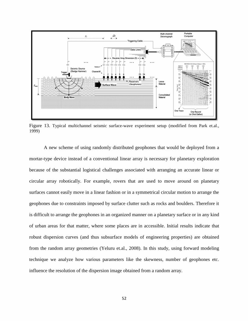
52
Figure 13. Typical multichannel seismic surface-wave experiment setup (modified from Park et.al.,
1999)
A new scheme of using randomly distributed geophones that would be deployed from a
mortar-type device instead of a conventional linear array is necessary for planetary exploration
because of the substantial logistical challenges associated with arranging an accurate linear or
circular array robotically. For example, rovers that are used to move around on planetary
surfaces cannot easily move in a linear fashion or in a symmetrical circular motion to arrange the
geophones due to constraints imposed by surface clutter such as rocks and boulders. Therefore it
is difficult to arrange the geophones in an organized manner on a planetary surface or in any kind
of urban areas for that matter, where some places are in accessible. Initial results indicate that
robust dispersion curves (and thus subsurface models of engineering properties) are obtained
from the random array geometries (Yeluru et.al., 2008). In this study, using forward modeling
technique we analyze how various parameters like the skewness, number of geophones etc.
influence the resolution of the dispersion image obtained from a random array.
53
Forward seismic modeling is a process through which a subsurface geologic model, in
one-two- or three dimensions, is transformed into a synthetic seismic record of one-two or three
dimensions. Synthetic seismic records are generated before and after the acquisition of seismic
field data. Synthetic seismic records generated before field acquisition are used to determine if
an intended/expected geologic target will generate an interpretable signature on output processed
seismic data. Synthetics can also be a valuable tool with respect to the design of an acquisition
program (for example; field acquisition parameters, sources, receivers etc.). The main idea
behind forward modeling is to generate synthetic seismograms for a given geologic model of the
subsurface and then compare it with the real seismic data acquired in the field. And if the two
data sets agree closely within an acceptable level of accuracy, the assumed geologic model is
considered to be a reasonably accurate model of the subsurface. If not, then the geologic model is
altered, and a new synthetic record is computed and compared. This process is continued,
iteratively, until a satisfactory match is obtained between the real and synthetic data. It is just the
opposite of inverse modeling approach in which geologic parameters are computed from real
data. But in reality, both the methods are used for the same goal-the determination of the
geologic structure and lithology of the subsurface.
4.2 MODELING PROGRAM OVERVIEW
The modeling software used in this study is 3-D eighth-order staggered-grid finite-
difference seismic modeling in anisotropic media using 21 elastic constants developed by the
University of Texas-Dallas (UTD). This program synthesizes 3-component common-source
particle velocity seismograms for a 3-D anisotropic media (21 elastic constants) using eighth-
order finite difference extrapolation on a staggered grid. The upper surface of the volume is
54
either the free surface (zero-stress) or an absorbing condition (using tapering). One run of the
program produces one three-component common-source gather for a set of receivers at any
specified locations, or for two intersecting linear arrays of receivers parallel to the horizontal
axes. Hudson’s (1980) second order scattering theory is used to parameterize media with dry or
fluid saturated crack systems (Martinez and McMechan, 2000). The complete system is coded in
Fortran 77, and has been tested in Unix environment using a SUN E6000. More detailed
explanation about the software can be found in the documentation (Martinez and McMechan,
2000). For this particular study, we set the surface to be a free surface (to obtain surface waves)
and used the vertical component of the shot gather. The three main input files for the program
include general.par, ucracks.par and model.index files. The general.par file contains the
parameters used by the modeling program such as the grid dimensions, time sample increment,
receiver positions, source parameters etc. The ucracks.par contains the output of the
parametrization program cracks. The model.index is an index file describing the structural
geometry of the earth model. Examples of the structure for each type of input file as used in this
study are shown in Appendix.
4.3 THEORY OF SURFACE WAVE PROPERTIES
Elastic properties of near-surface materials and their effects on seismic-wave propagation
are of fundamental interest in groundwater, engineering and environmental studies. In a
vertically heterogeneous medium, the phase velocity of surface waves is a function of frequency
(called dispersion curves). S-wave velocity is one of the key parameters in construction
engineering Rayleigh waves (Rayleigh, 1885) are surface waves that travel along a free surface.
They travel elliptical in a counterclockwise direction. The motion is constrained to a vertical

55
plane that is consistent with the direction of wave propagation. Therefore longer wavelengths
penetrate deeper than shorter wavelengths for a given mode and generally exhibit greater phase
velocities, and are more sensitive to the elastic properties of the deeper layers (Babuska and
Cara, 1991). On the other hand, shorter wavelengths are sensitive to the physical properties of
the surficial layers. Due to this reason, a particular mode of surface wave will possess a unique
phase velocity for each unique wavelength, leading to the dispersion of seismic signal. This
dispersion curve thus obtained from Rayleigh waves is a function of shear wave (S-wave)
velocity, layer thickness, density, and compressional wave (P-wave) velocity associated with
each geologic layer, listed in the decreasing order of priority (Xia et al. 1999). Therefore, it is in
principle possible to obtain S-wave velocity information from inverting the dispersive phase
velocity of the surface wave (Dorman and Ewing, 1962; Aki and Richards, 1980; Mari, 1984).
Rayleigh waves are non-dispersive in case of a solid homogeneous half-space and travels with a
velocity of approximately 0.9194 v1, if Poisson’s ratio is equal to 0.25, where v1 is the S-wave
velocity in the half-space (Sheriff and Geldart, 1985). However, they become dispersive when its
wavelengths are in the range of 1 to 30 times the layer thickness in case of layered earth model
(Stokoe et al., 1994). They travel at a velocity equal to 0.9194 v1 (where v1 is the S-wave velocity
of the layer) when the Rayleigh wave wavelengths are less than the layer thickness and they
travel at a velocity equal to 0.9194 v2 (where v2 is the S-wave velocity of the half-space) when
the wavelength exceeds 30 times depth of the half space.

56
4.4 CONSIDERATIONS FOR NUMERICAL SIMULATIONS
Rayleigh-wave dispersion curves for any layered
earth model (Figure 14) can be calculated by Knopoff’s
method (Schwab and Knopoff, 1972). Rayleigh-phase
velocity, CRj is determined by a characteristic equation F in
its nonlinear, implicit form:
F (fj,cRj,vs,vp,ρ,h)=0 (j = 1,2,….,m) ……..(7.1)
Where fj is the frequency, in Hz; cRj is the Rayleigh-wave
phase velocity at frequency fj ; vs = (vs1, vs2,…..vsn)T is the
S-wave velocity vector, with vsi the shear-wave velocity of
the ith layer; n is the number of layers; vp = (vp1,
vp2,…..vpn)T
is the compressional P-wave velocity vector,
with vpi the P-wave velocity of the ith layer; and ρ = (ρ1,
ρ2,…., ρn)T is the density vector, with ρi the density of the
ith layer.
So for a given set of model parameters (vs, vp, and ρ) and a specific frequency (fj), the roots of
equation (7.1) are the phase velocities. In this study, Hudson’s (1980) second-order scattering
formulism is used to compute the synthetic seismograms. A detailed work flow explaining
systematic procedure for generating dispersion image from the synthetic seismogram is shown in
Figure 15.
Figure 14: A 10-layered earth model
used in the modeling study

57
Table 4. Layered earth model parameters chosen from the dispersion
curve obtained from the field data
4.5 GROUP VS. PHASE VELOCITY ASSUMPTIONS
Surface waves are dispersive in nature, which mean that their velocities are a function of
frequency and that their group velocities are generally not equal to the phase velocities. Group
velocity (U=dω/dk) is the velocity in which the wave energy moves whereas phase velocity is
the velocity that a peak or trough moves.
For typical earth profiles, the phase velocity is generally faster than group velocity. While the
group velocity can increase or decrease with increasing period (as the wave is “stretched”), phase
velocities are monotonically increasing. Also, in case of highly anisotropic media, the group and
phase velocities are, in general, not equal and it is important to know whether the distance across
the sample divided by the travel time yields a phase velocity or a group velocity, as it makes a
substantial difference in the process of inverting velocities for stiffness of a material (e.g., the
MASW technique). Therefore care needs to be taken when choosing the appropriate parameter
for calculating the stiffness of materials.

58
Some laboratory experiments (Vestrum and Brown, 1994) show that group velocity inversions
are more complicated since the group velocity cannot be directly calculated in a prescribed
direction—and therefore adds computational complexity—but are easier to measure and yield
accurate results. On the other hand, phase velocity inversions are faster, more numerically
stable, and are easier to calculate but the results are not that accurate (Vestrum and Brown,
1994). In the same study, it was also concluded that there isn’t much difference between the
group and phase velocity measurements for a moderately anisotropic media, but there was
considerable difference while calculating stiffnesses of a higher anisotropic media.
In this study, however, assumption has been made, based on the known geology of the study area
(from exposure, trenching, and boreholes), that the subsurface is only moderately anisotropic.
Therefore, phase velocity measurements were used throughout the experiment as it was assumed
that there is not much potential advantage of using group velocity than phase velocity in surface
wave analysis, and also due to the fact that group velocities, although are more easy to measure,
has lower resolution than the phase velocity approach. In addition, processing the 2-D array data
using SURFSEIS (phase velocity approach) is a proven technique and there exists a lot of
literature already published on this methodology.
4.6 MODELING OF TYPICAL REGOLITH PROFILES
In order to test the sensitivity of the modeling software used in this study, an idealized
homogeneous half space (case-1) was considered for numerical simulations. Such model severs
as an important point of reference for any kind of parametric study. Along with the half space
model, three other cases were considered which are also very typical in real world. Case-2
represents a regular regolith profile where the stiffness of the layers increases with depth. This
situation is considered as normally dispersive regolith profile. Case-3 and case-4 represents more

59
realistic conditions where a soft layer is trapped in between two stiff layers and in another case a
stiff layer is trapped in between two soft layers. These conditions are considered as inversely
dispersive regolith profiles. As mentioned above, the important material properties that are
important to generate a dispersion curve are Vs, Vp, density, and thickness, therefore all these
property parameters for the four cases are all explained in Tables 5 through 8 respectively.
Figure 16 represents the 1-D shear wave velocity profiles obtained in all four cases. This initial
experiment suggests that this particular modeling software can be further be used to generate
dispersion curves for any case in varying conditions.
Table 5: Model for a homogeneous half-space
Table 6: Model for a regular regolith profile with stiffness of layers increasing with depth
Table 7: Model for irregular regolith profile with a soft layer trapped between two stiff layers

60
Table 8: Model for irregular regolith profile with stiff layer trapped between two soft layers
4.7 ANALYTICAL CONSIDERATIONS FOR DISPERSION CURVE ANALYSIS OF
RANDOM ARRAY MASW
In case of a 2-D geophone array (like cross, circular, or random) the imaging and analysis
of the dispersion curve deals with two main issues: 1) The sharpness of the image (which is
usually controlled or judged by the thickness of dispersion image bands), and 2) how accurately
it images the theoretical curves (we often observe some distortions at lowest frequency region of
the dispersion image). The second issue implicitly deals with what kind of computational
artifacts it generates. The resolution (sharpness) of the dispersion image is mainly controlled by
the total length (D) of the receiver spread, which in case of a 2-D array is the maximum length of
the array along the direction of the source. The length of the receiver spread (D) is directly
related to the longest wavelength (λmax) that can be analyzed from the dispersion curve, which
in turn determines the maximum depth of investigation (Zmax). The mathematical relations
associated with the above concepts can be expressed as;
D = mZmax (1 < m< 3) …….. (7.2)
Zmax= 0.5 λmax ………………(7.3)
61
On the other hand, the receiver spacing (dx) is related to the shortest wavelength (λmin) and
therefore determines the shallowest possible depth of investigation (Zmin). It is given by;
Zmin = kdx (0.3 < k < 1.0)….. (7.4)
The receiver spacing (dx) also determines the computational artifacts caused due to aliasing
effect. It sometimes generates some curved streaks in the dispersion image that is caused at the
point of dispersion where the wavelength becomes less than one half of dx. In case of random
array, since the separation between each geophone is not constant, we calculate dx to be the
minimum separation between two geophones, and this sometimes may cause the aliased streaks
in the image.
Therefore for any given random array geometry, the one that satisfies the conditions of
generating high resolution dispersion image that results in longer wavelength (λmax), is
considered to be the most optimum method that can be utilized for acquiring random array
MASW data.

62
Figure 15. Flow chart explaining step-by step process of modeling shot gathers

63
Figure 16. Shear wave velocity profiles for typical regolith profiles. Case1 represents an idealized
homogeneous half space. Case 2 represents regular regolith profile where stiffness of the layers
increases with depth. Case 3 represents irregular regolith profile where a soft layer is trapped in
between two stiff layers. Case 4 represents another irregular regolith profile where a stiff layer is
trapped in between two soft layers.

64
4.8 MODELING RESULTS
4.8.1 Clustered Array
Many naturally occurring spatial distributions show a pronounced tendency toward
clustering. Cluster analysis or Clustering, in general, means a group of the same or similar
elements gathered or occurring closely together, as a bunch. In general sense, the process of
clustering involves assigning a set of objects into groups (called clusters) so that the objects in
the same cluster are more similar to each other than to those in other clusters. In this experiment,
on the other hand, 48 random numbers were generated with different x-y coordinates and then
clustered in such a way that most of the geophones are grouped at one place except for few
scattered around inside the grid. Typical clustered arrangements used for this experiment are
shown in Figure 17. The earth model from Table 4 was used to generate seismograms for
clustered random array. Shot gathers and corresponding dispersion images obtained in all four
cases are shown in Figure 18. As can be observed from the cluster array figure, that out of the
four, the geophones in cluster 2 are least clustered and that of cluster 4 are most clustered.
The main aspects for comparing dispersion images for various arrangements, as
explained above, are the smoothness of the dispersion image/curve and the longest wavelength
(λmax) interpreted which ultimately determines the maximum depth of penetration (Zmax) of the
surface waves used for analysis. It is observed that the dispersion images pertaining to cluster 1,
2, and 3 do not cause any appreciable change in resolution except for cluster 4 which has lowest
resolution of all. The longest wavelength can be calculated from the dispersion curve extracted
from the image by selecting the phase velocity (C) pertaining to the lowest frequency (fmin) and
using the basic relation:
λmax = C/fmin ………(7.5)

65
Figure 17. Four different cluster array geometries used in the modeling. The X-axis
represents the E-W direction and Y-axis represents the N-S direction. The star represents
the shot point location (which is located at the origin).
Table 9 illustrates different λmax values obtained for different cluster arrays and it is
observed that cluster 2 has the highest and cluster 4 has the lowest λmax value. It can be observed
from figure 6 that out of the four geometries, cluster 2 is the least clustered and cluster 4 the most
clustered array. Therefore based on all the above facts, it can be interpreted that the less clustered
the receiver spread is the higher-resolution of the dispersion image and the deeper depth of
penetration (Zmax) will result in.

66
Figure 18. Shot gathers and corresponding dispersion images obtained for four different clustered
arrays. The X-axis represents frequency range 1-100 Hz and Y-axis represents phase velocity range
10-3000 m/s.

67
Figure 18. (contd…).

68
Table 9. Longest wavelength (λmax) and corresponding approximate depth of investigation
(Zmax) calculated for each type of configuration
4.8.2 Skewness Effect
In statistical terms, skewness is a measure of the symmetry of the probability distribution
of a real-valued random variable. The skewness value can be positive or negative, or even
undefined (from http://en.wikipedia.org/wiki/Skewness). A positive skew indicates that the mass
of the distribution is concentrated on the left side of the figure. It has relatively few high values
and the right tail is longer. A negative skew on the other hand indicates that the mass of the
distribution is concentrated on the right of the figure. It has relatively few low values and the left
tail is longer.
A zero value usually indicates that the values are relatively evenly distributed on both
sides of the mean, implying a symmetric distribution (http://en.wikipedia.org/wiki/Skewness).
Using this concept ninety-six (96) skewness values were generated using SPSS statistical
programming tool for normal, right, and left skew values. The distribution of the geophones
around the grid for all three cases is shown in Figure 19.

69
Figure 19: Graphical setup for the geophone coordinates as deployed around the grid for
normal, left and right skewed data. The star represents the source location (at origin) in all
three cases.
Such situation could be critical on any other kind of planetary surface, when there
might occur a case the geophones could all be skewed to either right or left. Figure 20
shows the shot gathers and the influence under the skewness condition on dispersion image
resolution. In this figure it can be observed that the normal skew data results in higher
resolution dispersion image for obvious reasons. But the images obtained from right and
left skew also shows a prominent dispersion image. Taking into consideration the fact that
the geometry pertaining to higher λmax value is considered to be the best possible one, the
dispersion curves for all three cases were processed for frequency range 1-100 Hz with 0.5
Hz increment and the phase velocity (C) for a range 10-3000m/s with 10 m/s increment.
The phase velocity (C) corresponding to fmin was determined. Then by using equation 5 the
longest wavelength travelled by surface waves in each case was calculated. It is observed in

70
this case (Table 9) that a normally skewed geophone arrangement yields the highest λmax
and posses the best resolution dispersion image.
4.8.3 Total Number of Traces
The total number of traces (N) takes into account the number of traces included in a
data set being analyzed for dispersion curves. It is also equal to the number of channels
used if one shot gather is being analyzed. Figure 21 illustrates the effect of N on resolution
of dispersion image and it is clearly observed that more number of traces results in higher
resolution. There are certain factors that can be associated with the total number of traces
like the length of spread (D), or the receiver spacing (dx) both of which were held constant
in this case. It has been examined from previous results (Park et.al., 2001) that a higher
number of channels can always result in high resolution dispersion image only when
accompanied by an increase in X and it is not of any benefit if we just increase N without
any increase in X. Also the receiver spacing (dx) should be long enough to result in a
receiver spread as long as possible. But too long receiver spacing would cause spatial
aliasing problems (Park et al., 2001)

71
Figure 20. Shot gathers for Normal, Left and Right skewed models and their corresponding
dispersion images. The X-axis on the dispersion image represents frequency (Hz) range 1-100 Hz
and the Y-axis represents phase velocity (m/s) range 10-3000 m/s.

72
Figure 21. Modeled shot gathers and corresponding dispersion images for different number of
channels. The X-axis represents frequency range 1-100 Hz and Y-axis represents phase-velocity
range 10-3000 m/s.
24 channel
48 channel
96 channel
73
4.9 DISCUSSION
In this study the influence of some key acquisition parameters pertaining to random array
geometry on the resolution of dispersion image has been examined. All the results were examined
and interpreted purely on theoretical basis explained in the previous sections. Although reliable
data results and key parameters concerning the acquisition design can be obtained from forward
modeling experiments, there are always other factors that need to be considered while collecting
real field data. Some of them include near and far field effects (Park et al., 1999), lateral
inhomogeneity in the subsurface and other surficial objects that may disturb the measurements.
Therefore all these factors should also be considered along with the parameters explained above
while determining the optimum parameters for a random array MASW survey. However, those
factors studied here are most critical from a data-processing perspective of generating accurate
dispersion images.
4.10 CONCLUSIONS
The following conclusions can be drawn based on formulistic perspective of the dispersion
curve analysis for a random array MASW survey.
The least clustered (more dispersed) random geometry is preferred in order to obtain higher
resolution dispersion image and a higher λmax.
A normally skewed geophone array yields a better resolution dispersion image and a higher
λmax.
A higher number of traces results in a higher resolution dispersion image, but it is
necessary to increase the number of traces only if you are increasing the area of coverage.
74
CHAPTER-5
Comparison of Seismic Surface Wave Dispersion Results Obtained from Conventional
versus Random Receiver Arrays
Note: This Chapter is written specifically to be submitted directly as a manuscript.
Therefore, there is some repeated material and overlap with previous and subsequent
chapters.
Yeluru, P.M., Baker, G.S., Perfect, E., and Park, C., in prep.
75
ABSTRACT
Understanding the physical and engineering properties within the upper 30 meters of any kind of
planetary subsurface will be critical as exploration advances and deployment of large structures,
and excavating for mining or human habitation on the earth and/or on other airless planetary
bodies becomes necessary. Advances in multi-channel seismic acquisition, either active or
passive, in acquiring reliable 1-D or 2-D shear wave velocity profiles have greatly improved our
ability to determine the engineering properties (e.g., Poisson’s ratio) of Earth’s shallow
subsurface, especially when using the seismic multi-channel analysis of surface waves (MASW)
technique. Using randomly distributed geophones (likely deployed from a mortar-type device)
instead of a conventional linear array is necessary due to the logistical constraints in arranging a
linear or circular array manually and/or robotically. Results indicate that robust dispersion curves
(and thus subsurface models of engineering properties) are obtained from the random array
geometries. Preliminary Geostatistical analyses also indicate that random array data can be used
to study spatial variations in geotechnical parameters of the subsurface. The goal of this study is
to compare this newly developed technique with that of the conventional methods in order to
evaluate for its accuracy. Multi-channel data is acquired using conventional arrays (e.g., linear,
circular and cross-arrays) at the same location where random data was collected. The dispersion
datasets, obtained using various conventional arrays, were consistent with data sets of the newly
developed array. All array methods are closely evaluated for the frequency, phase velocity, and,
shear wave velocity ranges; they all correlate well with one another. Random geometry is also
evaluated for potential improvements in the resolution of the dispersion image and as a more
accurate method for assessing azimuthal variations in the subsurface geology. More extensive

76
Geostatistical tools will be used to further analyze the data for any significant differences within
the patterns, and their interaction with depth.
5.1 INTRODUCTION
The geophysical technique of MASW is increasingly being applied to geotechnical
engineering for the measurements of dynamic properties like Poisson’s ratio distribution (Ivanov
et al., 2000a), seismic characterization of pavements (Park et.al., 2001a; Ryden et al., 2001), and
site characterization studies (Penumadu et.al., 2005). This technique is particularly used in
geotechnical engineering for measurements of shear wave velocity, identification of material
properties, their boundaries and spatial variations of ground etc. Being non-invasive and less
time consuming, the MASW method (Park et.al., 1999; Xia et.al., 1999) is used to evaluate
material layer thickness, shear wave velocity (1D and 2D), Poisson’s ratio and density. The
Multi-channel Analysis of Surface wave method (Park et.al., 1999) uses a multi-channel array,
which makes it possible to distinguish the fundamental-mode from higher modes and body
waves.
Depending on the source used to generate surface waves, there are two types of MASW
surveys: active method that utilizes a proper impact source like a sledge hammer and passive
method, on the other hand, utilizes ambient noise such as traffic or tidal motion. The active
method is considered to be the conventional mode of survey, collecting data in a roll-along mode
using an active seismic source and a linear receiver array. The passive remote method utilizes
ambient cultural noise such as traffic, thunder, tidal motion etc. and employs a two-dimensional
receiver array such as a cross, circular, random etc. to record passive surface waves.
Initial studies indicate that robust dispersion curves (and thus subsurface models of
engineering properties) can be obtained from random array geometries (Yeluru et al., 2008).
77
Using randomly distributed geophones (likely deployed from a mortar-type device) instead of a
conventional linear array is necessary due to the logistical constraints in arranging a linear or
circular array manually and/or robotically. It has been observed from preliminary experiments
that reliable dispersion images, and 1-D shear wave velocity profiles, can be obtained by using
random geophone arrangement.
However, a detailed statistical study comparing each different type of array and its effect
on dispersion analysis has not been reported yet. Therefore, this study is particularly focused on
comparing different types of conventional arrays with the random array in order to evaluate its
accuracy.
5.2 SITE DESCRIPTION-GEOLOGIC SETTING
The field Hydrology Teaching and Research Site is located at the University of
Tennessee (UT) Plant Science Farm, alongside Highway approximately 2 miles south of the UT
campus (Figure 22). It is located between the highway and the Tennessee River. Regolith
conditions across the site vary from residual regoliths developed directly on sedimentary bedrock
near the highway, to loamy regoliths developed on a series of alluvial terraces at different
elevations above the river. Both visual and particle size analyses of sediment sampled from two
borings support this fining up progression. Analysis of material from existing core samples from
wells drilled at this location further confirms this progression. The bedrock is very fine-grained
Ordovician calcareous Ottossee Shale, underlying the sediment at the site and is composed of
claystone, shale and sandstone depositional sequences with some limestone interbeds. The upper
portion of the bedrock contains numerous weathered and stained fractures and can also be used
as a low yield aquifer. Also the underlying irregular and heterogeneous bedrock surface was

78
reworked under high energy conditions as coarse sands and gravel were laid down. The contact
between the Ottosee Shale and the alluvium was found to be weathered bedrock beneath
unconsolidated coarse gravel and sand material. Clays from the hydrogeology teaching and
research site sampled from core samples were calcareous with weathered shale fragments. The
variable types of clay can be attributed to the folded and interbedded shale, sandstone, and
limestone bedrock underlying the field site (Benfield et al., 2003).
Figure 22. Location of the University of Tennessee Agricultural Extension Center, Knoxville, TN.
The yellow square located in the zoomed in map shows the location of the study area (Google
Earth).

79
5.3 DATA ACQUISITION AND ANALYSIS
Data Acquisition
The MASW data were collected for linear, circular, cross and random arrays at the
University of Tennessee agricultural field test site in eastern Tennessee USA, using 2, 24-
channel Geometrics Geode seismograph with 40 Hz spike coupled geophones with spike firmly
planted on the ground. The data were collected in SEG2 format with a recording time of 1000 ms
and sample interval of 0.5ms. Other parameters like the source-receiver offset distance, total
length of the array line and receiver spacing were all estimated depending upon the array type.
Acoustic energy was generated by using a 10-lb sledge hammer and metal plate as the seismic
source and the data were acquired at 13 different shot points around the 10 m × 10 m grid. No
acquisition frequency filter was applied during the recording. To increase signal-to-noise ratio, three
impacts at each station were vertically stacked. The receiver array lengths varied depending on the
array design but they all shared the same center point. The dimensions and other parameters used
for each type of receiver array are described in Table 10. Also the grid setup and the locations of
the shot points are all portrayed in Figure 23. Four different random data sets were collected (all
having different X-Y coordinates) in order to determine the repeatability of the method. Typical
shot gathers for each type of array as acquired in the field are shown in Figure 24. Also a
schematic representation of various array designs as deployed within the 10 m × 10 m grid in the
field are shown in Figure 25 (a)-(b).

80
Figure 23. The figure on the left represents the shot point locations as deployed on the ground.
There are total 13 shot points from which data was collected. The distance between each shot
point location is 10 m. The figure on the right represents the random arrangement of geophones
(small circles) inside a 10 m×10 m grid.
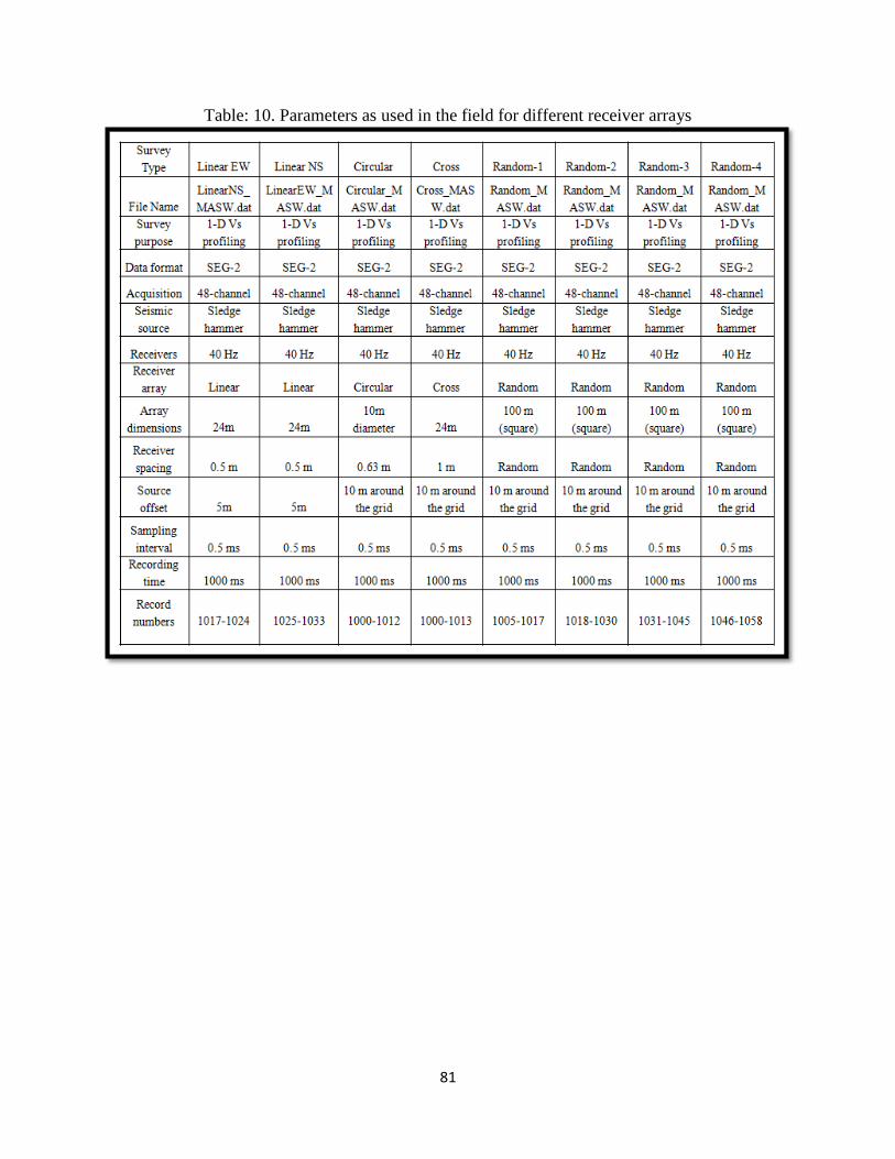
81
Table: 10. Parameters as used in the field for different receiver arrays

82
Figure 24. Shot gathers for various arrays. The X-axis represents offset (m) and trace numbers and
Y-axis represents time (ms). Data was collected for 1000ms but only the first 500ms is shown
here.

83
Figure 25 (a). Schematic representation of various array designs as deployed in the field. The X-
axis represents E-W and Y-axis represents the N-S directions. Each square represents the 10 by 10
grid and 13 shot points were deployed around this grid whose locations are shown in Figure 23.
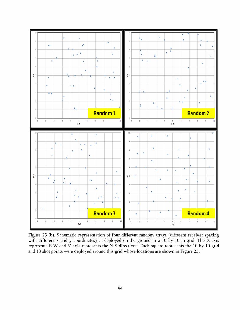
84
Figure 25 (b). Schematic representation of four different random arrays (different receiver spacing
with different x and y coordinates) as deployed on the ground in a 10 by 10 m grid. The X-axis
represents E-W and Y-axis represents the N-S directions. Each square represents the 10 by 10 grid
and 13 shot points were deployed around this grid whose locations are shown in Figure 23.

85
Data Analysis
The obtained surface wave data were processed using SURFSEIS software developed by Kansas
Geologic Survey and involved the following process. The overall procedure involved in the
processing of surface wave data with various receiver arrays using the XY coding module is
explained in the flow chart shown in Figure 26. The XY coding module developed by Park
Seismic LLC is a receiver array coding system that inserts receiver coordinates (X and Y) into
corresponding trace headers. Distance (offset) from source is also calculated based on the
relative coordinates between source and receiver and stored in the proper trace header. It takes
the receiver ARRAY file (*.txt) created from SurfSeis array map and the seismic source
coordinates as inputs. Arbitrary station numbers are assigned into each trace with source point
being station #1000 and each trace’s station #’s being 1000+channel#. A screenshot image of the
module is shown in Figure 27. In step 1, we upload the desired shot record. In step 2, we insert
the receiver array text file. In step 3, we designate a place to save the output. In step 4, we enter
the source coordinates corresponding to the shot gather uploaded in step 1. This process is
repeated for each shot gather of a particular receiver array. Once the fieldsetup is applied
following the above process, the shot gathers were further used to extract dispersion images for
various receiver arrays using the SURFSEIS software in the traditional way.
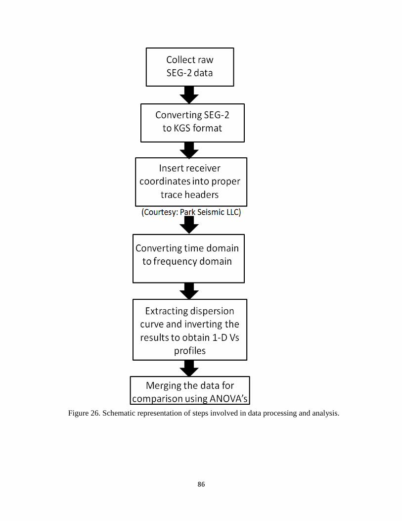
86
Figure 26. Schematic representation of steps involved in data processing and analysis.

87
Figure 27: A screenshot image of the receiver coding module that was used in 2-D receiver array
processing.
An average dispersion curve was obtained by combining all 13 records using frequency
range 1-100 Hz and phase velocity range 10-3000 m/s. This process was repeated for all receiver
array types and the dominant frequency of surface waves varied around 30-55 Hz for different
arrays. A very good signal to noise ratio was obtained for all records. The dispersion images
obtained for various conventional arrays and for four different random arrays are shown in
Figure 28 (a)-(b). It can be observed that the dispersion of the fundamental mode of surface
waves is very clear in the frequency range from 10-40 Hz for conventional arrays but the
fundamental mode extends only up to 30 Hz for random array (Figure 29) with a steep decrease
of phase velocity in the range 12-17 Hz down to minimum phase velocity of around 340 m/s. No
Rayleigh wave energy is found propagating lower than 10 Hz and this part of the dispersion

88
image appears blank for all array types. Part of the reason for this observation may be the
presence of stiff basement rocks. In some of the dispersion images some higher modes of surface
waves are clearly visible above 18 Hz. Once the bounds (upper and lower limits of phase
velocities for the dispersion curve to be extracted) are set, the dispersion curve is extracted
automatically within the given range. The total number of dispersion picks that constitutes the
dispersion curve was set to 30 with equal-wavelength frequency interval used to make the
frequency interval denser at low and coarser at higher frequencies. The dispersion curves
extracted for various conventional and random array agreed closely especially at frequencies
between 10-18 Hz although there were discrepancies at higher frequencies around 20-32 Hz
between the conventional arrays and the random array (Figure 30). It can also be observed that
out of the four different random arrays, the dispersion image corresponding to random 4 is
crisper and the fundamental mode can be more readily identified in it when compared to the
other random array images. A graphical representation of the dispersion picks (Figure 31) for
the four random arrays show that random 4 is different from random 1, 2, and 3 in a way that the
fundamental mode for random 4 starts around 10 Hz and extends up to 32 Hz, which closely
resembles the conventional arrays whereas random 1, 2, and 3 starts around 14 Hz and extends
up to 32 Hz. This deviation might have occurred due to over estimated phase velocities, which is
a typical phenomenon caused by dominating energy from higher modes (Park et al., 1999).
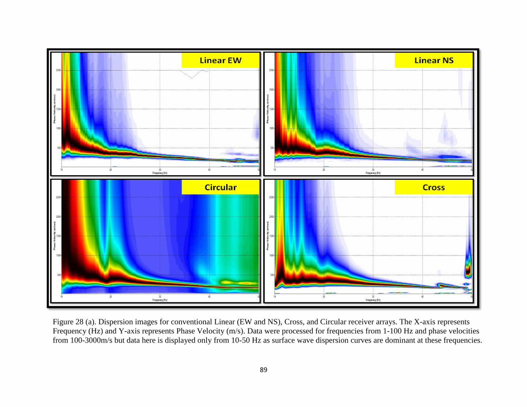
89
Figure 28 (a). Dispersion images for conventional Linear (EW and NS), Cross, and Circular receiver arrays. The X-axis represents
Frequency (Hz) and Y-axis represents Phase Velocity (m/s). Data were processed for frequencies from 1-100 Hz and phase velocities
from 100-3000m/s but data here is displayed only from 10-50 Hz as surface wave dispersion curves are dominant at these frequencies.
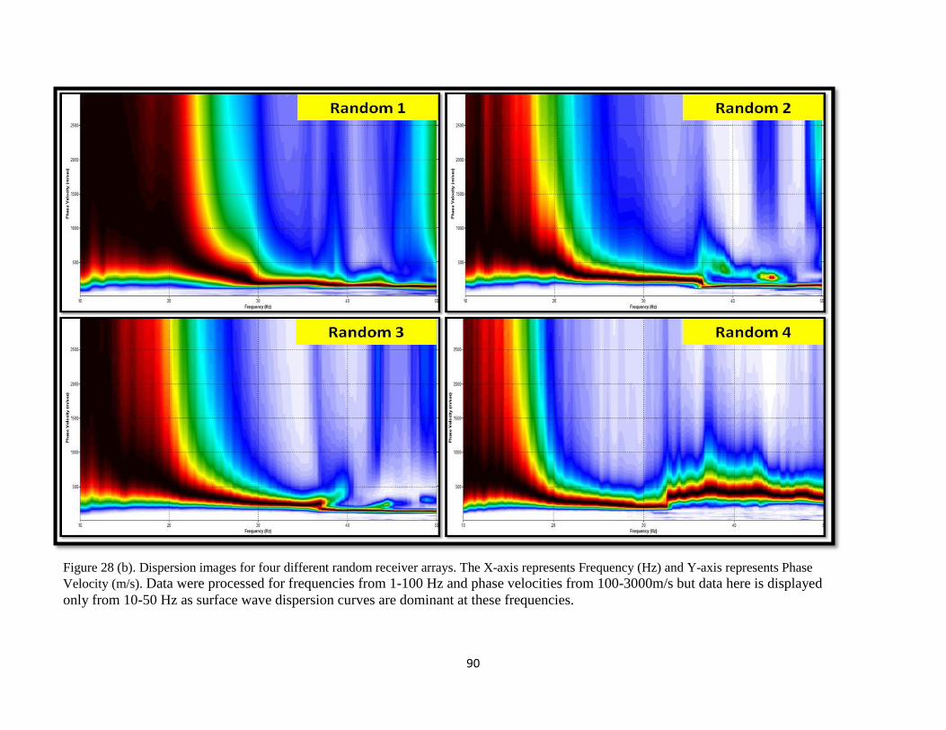
90
Figure 28 (b). Dispersion images for four different random receiver arrays. The X-axis represents Frequency (Hz) and Y-axis represents Phase
Velocity (m/s). Data were processed for frequencies from 1-100 Hz and phase velocities from 100-3000m/s but data here is displayed
only from 10-50 Hz as surface wave dispersion curves are dominant at these frequencies.

91
Figure 29. A graph representing dispersion curve comparison for four types of
receiver arrays. The X-axis represents frequency (Hz) ranging from 10-40 Hz
and Y-axis represents phase-velocity (m/s) ranging from 0-1000 m/s.
Figure 30. Comparison of dispersion curves for various random array
distributions. The X-axis represents frequency (Hz) ranging from 10-35 Hz and
Y-axis represents phase-velocity (m/s) from 0-1000 m/s. It is observed that
random 1, 2, and 3 curves show higher velocity values when compared to
random 4.
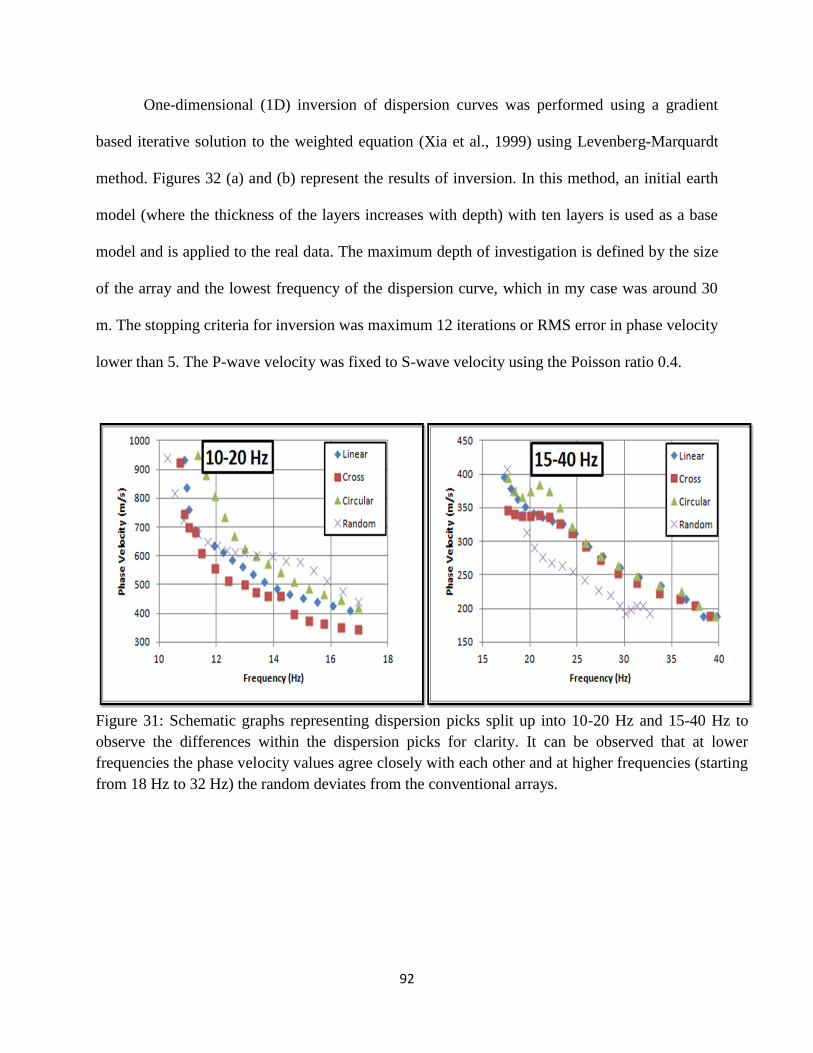
92
One-dimensional (1D) inversion of dispersion curves was performed using a gradient
based iterative solution to the weighted equation (Xia et al., 1999) using Levenberg-Marquardt
method. Figures 32 (a) and (b) represent the results of inversion. In this method, an initial earth
model (where the thickness of the layers increases with depth) with ten layers is used as a base
model and is applied to the real data. The maximum depth of investigation is defined by the size
of the array and the lowest frequency of the dispersion curve, which in my case was around 30
m. The stopping criteria for inversion was maximum 12 iterations or RMS error in phase velocity
lower than 5. The P-wave velocity was fixed to S-wave velocity using the Poisson ratio 0.4.
Figure 31: Schematic graphs representing dispersion picks split up into 10-20 Hz and 15-40 Hz to
observe the differences within the dispersion picks for clarity. It can be observed that at lower
frequencies the phase velocity values agree closely with each other and at higher frequencies (starting
from 18 Hz to 32 Hz) the random deviates from the conventional arrays.
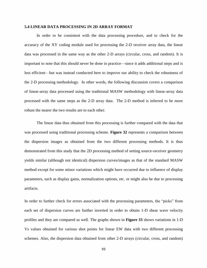
93
5.4 LINEAR DATA PROCESSING IN 2D ARRAY FORMAT
In order to be consistent with the data processing procedure, and to check for the
accuracy of the XY coding module used for processing the 2-D receiver array data, the linear
data was processed in the same way as the other 2-D arrays (circular, cross, and random). It is
important to note that this should never be done in practice—since it adds additional steps and is
less efficient—but was instead conducted here to improve our ability to check the robustness of
the 2-D processing methodology. In other words, the following discussion covers a comparison
of linear-array data processed using the traditional MASW methodology with linear-array data
processed with the same steps as the 2-D array data. The 2-D method is inferred to be more
robust the nearer the two results are to each other.
The linear data thus obtained from this processing is further compared with the data that
was processed using traditional processing scheme. Figure 32 represents a comparison between
the dispersion images as obtained from the two different processing methods. It is thus
demonstrated from this study that the 2D processing method of setting source-receiver geometry
yields similar (although not identical) dispersion curves/images as that of the standard MASW
method except for some minor variations which might have occurred due to influence of display
parameters, such as display gains, normalization options, etc. or might also be due to processing
artifacts.
In order to further check for errors associated with the processing parameters, the “picks” from
each set of dispersion curves are further inverted in order to obtain 1-D shear wave velocity
profiles and they are compared as well. The graphs shown in Figure 33 shows variations in 1-D
Vs values obtained for various shot points for linear EW data with two different processing
schemes. Also, the dispersion data obtained from other 2-D arrays (circular, cross, and random)

94
were also compared with the linear EW data (both 1-D and 2-D processing) and the results are
shown in Figure 34.
Figure 32: Dispersion images for selected shot records from linear EW data. The image on the left
was processed using the traditional MASW processing scheme and the image on the right was
processed using the XY coding module. The X-axis represents Frequency (Hz) and Y-axis represents
Phase-velocity (m/s).
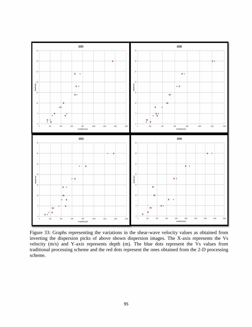
95
Figure 33: Graphs representing the variations in the shear-wave velocity values as obtained from
inverting the dispersion picks of above shown dispersion images. The X-axis represents the Vs
velocity (m/s) and Y-axis represents depth (m). The blue dots represent the Vs values from
traditional processing scheme and the red dots represent the ones obtained from the 2-D processing
scheme.

96
Figure 34: Graphical representation of variations in dispersion curves for various
receiver arrays with the two types of processing schemes. The X-axis represents
Frequency (Hz) and Y-axis represents Phase-velocity (m/s).

97
5.5 RESULTS
The 1-D shear wave velocity profiles obtained with different types of arrays are shown in
Figures 35 (a)-(b). The variation of Vs velocities at all depths seems to be pretty consistent for
all array types. The depth to the bedrock can be clearly identified at around 12 m depth from all
array types. Figure 38 (a) represents a regolith profile obtained on the test site using cross hole
and borehole data. The obtained was compared both graphically (Figures 36 and 37),
statistically (Table 11 and 12) and also from the 1-D Vs profiles (Figure 35 a-b).
Comparison of velocity profiles up to a depth of 30 m shows the following results:
a) All the profiles start with thin layer (1-2m thick) and are characterized by MASW shear-
wave velocities between 200-400 m/s on an average for all array types. This zone
primarily consists of low plasticity organic silts.
b) In the depth range of 2-3 m there is a low velocity layer (130-190 m/s) which is
prominent in almost all the profiles. This layer is characterized by silts that grades to silty
sand. It is observed from the core samples taken from the site that the silt and sand layers
are laterally extensive.
c) It can also be observed from the Vs profiles that there is a slight decrease in the velocities
at 7.5-10 m depth and this might be due to the transition of silt to sand. This transition
depth can also be verified from the particle size analysis that was done on the core data
acquired from this site (Benfield et al., 2003). These tests were done at several depths and
the one done on the 7.5 m sample showed that the fine material begins to grade to sand
and further grades to coarser sand and gravel.
d) After approximately 10 m depth (at around 12 m) the shear wave velocity values increase
gradually until 30m from 375 m/s to 880 m/s in linear array, 400 m/s to 1000 m/s for

98
cross, 500 m/s to 975 m/s for circular and from approximately 400 m/s to 900 m/s in
random. This increase in velocity values may correspond to either clay or saprolite
formation above bed rock. Also the highest velocity found in the inversion was around
900 m/s indicative for bedrock which is characterized by calcareous shale with some
limestone interbeds.
Although there are variations within each array with respect to each depth, the S-velocities
from dispersion of surface waves for all the depths on an average are comparable with each other
and determine geologically similar results. The average shear-wave velocity in upper 30 m
(Vs,30) which is a parameter widely applied in seismic microzonation, also the main parameter
for ground type classification in Eurocode 8 standard (EUROCODE 8, 2003), was computed using
the following expression for each array type.
Where hi and Vi denote the thickness (in m) and shear-wave velocity (in m/s) in the i-th
formation of layer, in a total of N, existing in the top 30 meters. The following values were
obtained for each array:
…… (6.1)

99
It can be inferred from the above values that the investigated site is classified as ground
type E (Vs<180 m/s) from all different types of arrays which is a characteristic of soft regoliths
except for random arrays 1, 2, and 3 which are characterized more as stiff regolith and not soft
regolith. They show higher values as an effect of overestimated phase velocity values in the
dispersion curves. Considering also the stratigraphic description of the site (Figure 38 a) as well
as the Vs 30 values the ground type is described as: quaternary alluvial deposits exhibiting
coarse gravel materials grading upward to finer texture sands and silts.

100
Figure 35 (a). 1-D shear wave velocity profiles for various conventional and random receiver arrays obtained by
inverting the phase velocity picks from Figure 28 (a).
Figure 35 (b). 1-D shear wave velocity profiles for various random arrays obtained by inverting the phase velocity
picks from figure 28 (b).
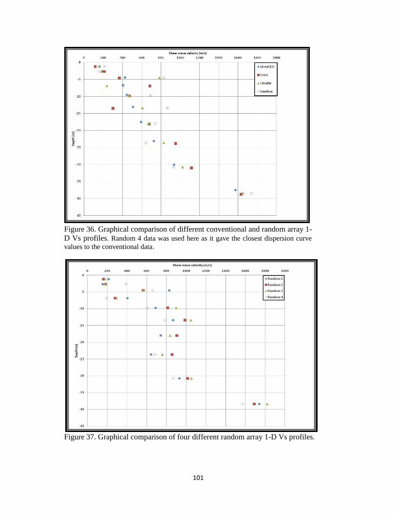
101
Figure 36. Graphical comparison of different conventional and random array 1-
D Vs profiles. Random 4 data was used here as it gave the closest dispersion curve
values to the conventional data.
Figure 37. Graphical comparison of four different random array 1-D Vs profiles.
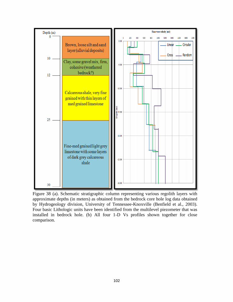
102
Figure 38 (a). Schematic stratigraphic column representing various regolith layers with
approximate depths (in meters) as obtained from the bedrock core hole log data obtained
by Hydrogeology division, University of Tennessee-Knoxville (Benfield et al., 2003).
Four basic Lithologic units have been identified from the multilevel piezometer that was
installed in bedrock hole. (b) All four 1-D Vs profiles shown together for close
comparison.

103
5.6 STATISTICAL ANALYSIS
In order to further compare the datasets obtained from different arrays in more
quantitative way, analysis of variance (ANOVA) was performed on all eight data sets for
inversion data using SAS programming tool (Output attached in Appendix). The GLM procedure
was used to analyze the data. The results showing significance levels for various models and the
interaction between different geophone patterns with different variables (for example; depth vs.
shear-wave velocity) are tabulated in Tables 11 (a), (b), (c), and (d).
Table 11 (a) shows the significance levels and error terms associated with the assumed model.
The main effects and interactions of different patterns and depth, which were both considered as
fixed factors here, were tested within each block and the output is attached in the Appendix.
Multiple comparisons were run for depth and pattern, as well as their interaction so we can find
the pattern effect in each condition of depth and vice versa. In the table, pattern represents the
geophone arrangement (linear, circular, cross, and random). Rep data was first included in the
analysis as a factor but since it showed no significant difference at the p < 0.05 confidence level,
it was removed and the model was re run without rep specified. Table 11 (b) indicates there
were significant effects due to depth, pattern, and pattern * depth with respect to the Vs data.
Figure 39 represents the interaction plot for Vs with pattern for various depths.
It is clearly observed from the ANOVA analysis that there were significant effect of both
pattern and pattern * depth at the p < 0.05 probability level i.e., some of the random patterns
were significantly different from the other patterns at certain depths. The F-values for pattern and
pattern * depth were considerably less than the F-value for depth, indicating that depth was the
most important source of variation in these data. However, since the effect of pattern * depth was
significant there is a need to compare individual patterns with each other by depth. The

104
conclusion from this analysis is that, although the effects of pattern and pattern * depth were
small relative to depth, they were statistically highly significant which means that some random
patterns at certain depths will yield different Vs results from other random patterns and/or
conventional sampling arrays.
5.7 CONCLUSIONS
Performed investigations of comparing the newly developed random array with four
different types of MASW geophone arrays have shown that they are all quite effective in
determining shallow shear-wave velocity profiles and that the results obtained from random
array are comparable with that of the conventional arrays upto a certain extent. However, this is
true up to a certain extent only if various aspects such as those described in chapter-3 are
considered while deploying a random array. The average shear-wave velocity in the 30 m thick
layer of sediments is between 140 m/s to 155 m/s characterizing the regolith to be soft regolith.
The depth to the bedrock could be identified at approximately 12 m depth in all receiver array
types including the newly developed random array. It is also inferred from the field experiments
that the more dispersive the geophones are in a random array, the better the resolution of the
dispersion image, and thus the 1-D Vs interpretations. It can be concluded thus from the
comparison of various receiver arrays, the estimated bedrock depths and proximal ground truth,
that the interpretation of the 1-D MASW shear-wave velocity profiles from different array types
is reasonably reliable and the random array profiles are quite comparable with that of the
conventional to an acceptable level. The implication is that the dispersion curves from various
conventional and random receiver arrays are also reliable. It should be noted, however, that other
random array realizations can result in significantly different results compared to those from
conventional arrays. Therefore care should be taken while deploying a random array and various

105
different aspects such as skewness, clusteredness, etc. should be considered while performing
random array MASW survey.
Table 11. Statistical (mixed model analysis) analysis performed on inversion data using SAS
programming with dependent variable Vs (shear-wave velocity).
(a)
(b)
Figure 39: Interaction plot for Vs with depth for different geophone arrays.

106
CHAPTER-6
Adapting a random-array acquisition scheme for a seismic surface-wave study of a
terrestrial analog site at Black Point Lava Flow, Arizona USA, as a potential rover-friendly
methodology
Note: This Chapter is written specifically to be submitted directly as a manuscript.
Therefore, there is some repeated material and overlap with previous and subsequent
chapters.
Yeluru, P.M., Baker, G.S., Park, C.B., and Perfect, E. in prep.

107
ABSTRACT
Subsurface imaging is very critical to exploit subsurface resources, monitor the fluid movement
in the reservoir, mapping tunnels etc. As science advances scientists and other researchers are
constantly trying to develop new techniques and methods for subsurface imaging that are more
effective, efficient, and are more robust under varying field conditions. Advances in near-surface
geophysical techniques, such as multi-channel analysis of surface waves (MASW), have greatly
increased our ability to map subsurface variations in physical properties here on Earth. The
MASW method involves deployment of multiple seismometers to acquire 1-D or 2-D shear wave
velocity profiles that can be directly related to various engineering properties. Initial experiments
have determined that the MASW method when used along with random geophone arrangement
can successfully delineate subsurface features and properties. The purpose of the research
presented here is to demonstrate the usefulness and capabilities of MASW technique at terrestrial
site (the Black Point Lava Flow) where the geologic settings, processes, and materials are very
different from that of the controlled site in Knoxville, TN. The regolith at the controlled site are
more consolidated sands whereas the regolith at the BPLF site is more unconsolidated and the
whole area is filled with basaltic rocks formed by a 2 million year old lava deposits. The results
focus on near-surface MASW studies and interpretation of the subsurface geology using a
random geophone array. The novel random array scheme presented here will likely be necessary
for any kind of future off-Earth exploration because of the logistical constraints involved in
deploying more traditional linear or circular arrays manually and/or robotically.
108
6.1 INTRODUCTION
Multichannel analysis of surface waves (MASW) data collected from terrestrial
environments will likely be critical for pre- or sys-arrival of astronauts at semi-permanent
habitation sites involving mining, protection caves, or landing of large craft. . Ultimately, if
deployed on non-Earth locations, the MASW technique can yield insight into mapping
subsurface variations in physical properties, and other important engineering properties of the
subsurface—like shear modulus, shear wave velocity and Poisson’s ratio (Park et al., 1999), that
are the key parameters for any type of civil engineering works, as they characterize the
mechanical behavior of geotechnical materials under various types of loading. Multi-channel
surface wave data was collected at Black Point Lava Flow (BPLF) site which is 40 km north of
Flagstaff, Arizona in March 2012. This field test was primarily intended to determine the
engineering parameters, like shear wave velocities, at a high-fidelity simulant using MASW
method with randomly distributed geophone arrangement. Such type of array will be necessary
for future planetary exploration keeping in mind the logistical constraints involved in deploying
a linear or circular array manually and/or robotically. An initial study (Yeluru et al., 2008) has
proven that robust and reliable dispersion images could be obtained using random geophone
array. The field techniques discussed here, although applicable on Earth, is also intended for
surfaces and regolith in the future exploration of planetary bodies for possible human habitation.
This would include Mars, its Moon-Phobus/Deimos, Near-Earth Asteroids (NEA’s), even
Earth’s Moon. With each situation, the nature of the regolith and its formational processes will
place certain restrictions and limitations upon the applications. This is expected with any change
of terrains even on the Earth, let alone between planetary bodies. Here, I present a description of
the experiment conducted and the results thus obtained.

109
6.2 TERRESTRIAL ANALOG SITES FOR SEISMIC STUDIES
Analog sites are places or spaces on earth that approximate, in some respect, the geological,
environmental and putative biological conditions or settings on a particular planetary body,
either at the present day or sometime in the past (from en.wikipedia.org/terrestrial analogue
sites). Therefore, an analog may be broadly defined based on the conditions the site is meant to
represent and the specific parameters meant to be examined/tested. For example, a meteoritic
impact crater site is an obvious analog for the moon where surface geometry, etc. are of interest,
whereas a basalt lava plateau that has undergone severe physical weathering is an equally
legitimate analog site if the physical properties of the subsurface are of interest. The use of a
terrestrial test site that has properties approximating of what may exist on any planetary body
such as moon, is an essential component in the development of systems that are planned for
planetary and planetary exploration. Also such experiments help aid astronauts, engineers and
scientists to enhance scientific exploration by combining human and robotic efforts. Such test
sites can be used to test robotics, vehicles, habitats and in-situ resource utilization in realistic
environments that will help us better prepare and understand the complex challenges that will be
encountered on a planetary surface.
Selecting a test site that best approximates of what may exist on the moon in terms of
engineering and geotechnical properties and that would best suit my proposed research is an
integral element, capable of influencing data and impacting test results. Examples of relevant
characteristics of some field test sites for my work include terrains, regolith properties,
meteorology, geologic features, biological changes and remoteness. Investigation of surface
processes and comparative studies with other planetary bodies can be carried out using several
techniques and methods including, but not limited to, (1) fieldwork and remote-sensing

110
campaigns at terrestrial analog sites; (2) comparisons between terrestrial and planetary datasets;
and (3) numerical and computer modeling of geological processes (Tornabene et al.,2005).
Various locations that can serve as a test site that approximates what may exist on the moon in
terms of physical properties are explained below (from www.nasa.gov).
Antarctic
These kinds of places are mainly used to test the inflatable habitat concept. When astronauts
return to the moon for extended stays, they will require shelter to live and work under for
protection from the harsh planetary environment. The site selected was the cold, isolated
landscape of Antarctica.
Oceans
Ocean conditions such as the Florida Keys National Marine Sanctuary, serves as a test site for
NASA’s Extreme Environment Mission Operations. NASA uses the laboratory’s planetary-like
environment as a semi-permanent site for testing planetary exploration concepts such as
advanced navigation and communication equipment. Astronauts also execute a variety of
undersea “moonwalks” at this site. The tests cultivate an astronauts understanding of his or her
ability to carry out daily operations in a simulated planetary environment.
Deserts
These sites are used to measure the benefits of using pressurized vehicles as opposed to
unpressurized vehicles, and incorporate the findings into upcoming planetary missions. These
sites are also needed to conduct short-distance mobility exploration and also engineering
evaluation tests to investigate the utility of its robotic vehicle concepts in an earthly moonscape.
For this purpose NASA found the sand dunes of Moses lake, Washington. And the desert-like

111
landscape in Black Point Lava flow, Arizona is well suited for testing technologies and
procedures for future human-robotic exploration in extreme environments.
Volcanic Terrains
The terrain, rock distribution and regolith materials at such sites as in Hawaii and Idaho provide
an ideal simulated environment for testing hardware and other equipment to harness local
resources for use in human and robotic exploration.
A few of the many terrestrial analog sites, within United States were studied in detail and the
Black Point Lava Flow (BPLF) site was selected.
6.3 GEOLOGIC SETTING-BLACK POINT LAVA FLOW
The San Francisco volcanic field is an area of volcanoes in northern Arizona, north of
Flagstaff, USA. This field contains approximately 600 volcanoes in age from less than 6 million
years old to less than 1,000 years (Miocene to Holocene). The Black Point Lava Flow (BPLF) is
a part of the San Francisco volcanic field which is approximately 2 million years old (from
en.wikipedia.org/San Francisco field site). Stretched across much of the northern Arizona, the
Black Point Lava Flow resembles an alien landscape on Earth, the perfect place for NASA to test
rovers, habitats, space suits and the other equipment that future astronauts will need when they
explore the moon, the asteroids as well as Mars and the Moons of the Red Planet (from
http://spacecoalition.com). It is considered one of the best and excellent sites for surface system
analog sites, because it shares so many terrain and environmental similarities with the Moon,
Mars, and near Earth asteroids (from www.nasa.gov). Like so many other planetary bodies,
Black Point Lava Flow is a desolate environment with rugged terrain, dust storms, varying
regolith composition, temperature extremes, deep craters, steep slopes, rolling plains, and
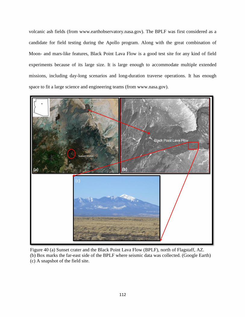
112
volcanic ash fields (from www.earthobservatory.nasa.gov). The BPLF was first considered as a
candidate for field testing during the Apollo program. Along with the great combination of
Moon- and mars-like features, Black Point Lava Flow is a good test site for any kind of field
experiments because of its large size. It is large enough to accommodate multiple extended
missions, including day-long scenarios and long-duration traverse operations. It has enough
space to fit a large science and engineering teams (from www.nasa.gov).
Figure 40 (a) Sunset crater and the Black Point Lava Flow (BPLF), north of Flagstaff, AZ.
(b) Box marks the far-east side of the BPLF where seismic data was collected. (Google Earth)
(c) A snapshot of the field site.
(a) (b)
(c)
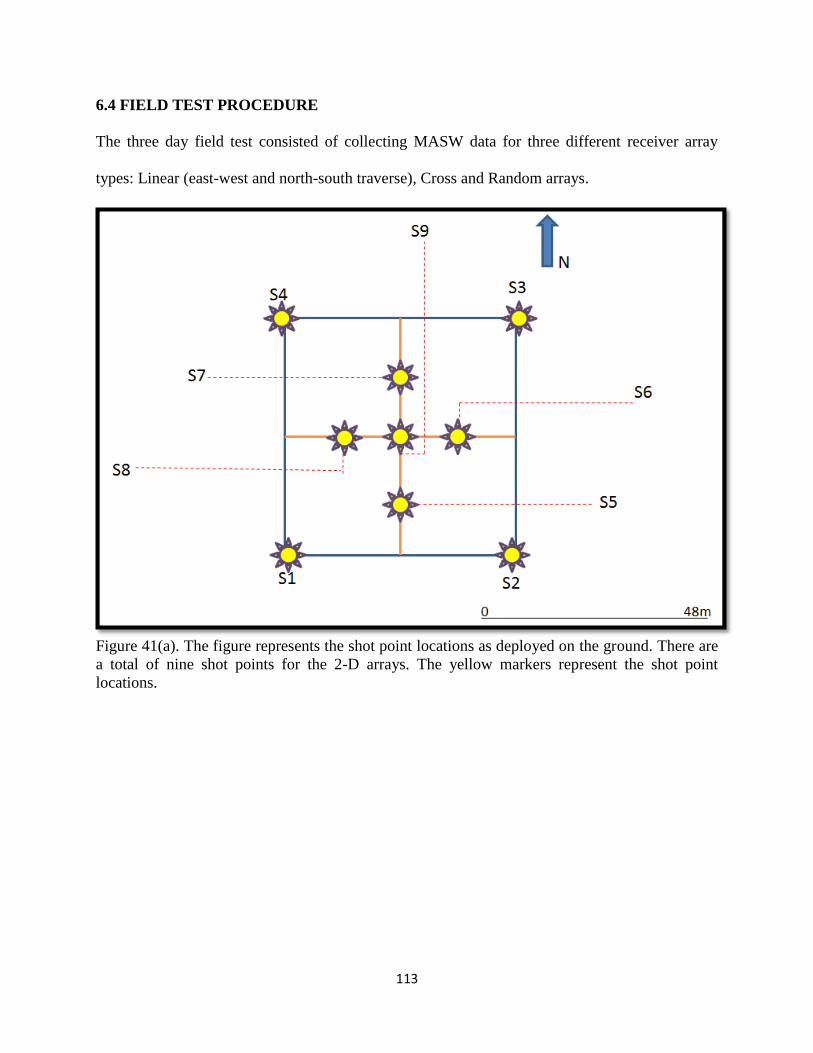
113
6.4 FIELD TEST PROCEDURE
The three day field test consisted of collecting MASW data for three different receiver array
types: Linear (east-west and north-south traverse), Cross and Random arrays.
Figure 41(a). The figure represents the shot point locations as deployed on the ground. There are
a total of nine shot points for the 2-D arrays. The yellow markers represent the shot point
locations.

114
Figure 41(b). Schematic representation of various receiver arrays as deployed in the
field. X- axis represents E-W traverse and Y-axis represents N-S traverse (i) Linear EW
(ii) Linear NS (iii) Cross (iv) Random.
Data acquisition
Multi channel data were collected on the BPLF site in Flagstaff, Arizona, using a 96-
channel Geometrics start view seismograph with 14 Hz geophones. A 10-lb sledge hammer was
used as a seismic source to generate source energy and data was collected on a 48m×48m grid
(Figure 41a). Fifteen shot records (not shown in Figure 33) were shot for the linear arrays (EW and
NS traverses) and nine records were shot for cross and random arrays (shown in Figure 41a).
Graphical representations of various arrays are shown in Figure 41b and a summary of data
acquisition parameters are tabulated in Table 12. A time sampling interval of 0.5 ms and a total
(i) (ii)
(iii) (iv)

115
recording time of 1000 ms were used during data acquisition. No acquisition filter was applied
during the recording. Three sets of data were collected for each array. A typical shot gather for
each type of array are represented in Figure 42.
Figure 42. Typical shot gathers for various array types as acquired from the BPLF field site.
Data was collected for 1000 ms but only the first 500 ms data is shown here as surface waves
are more prominent here.
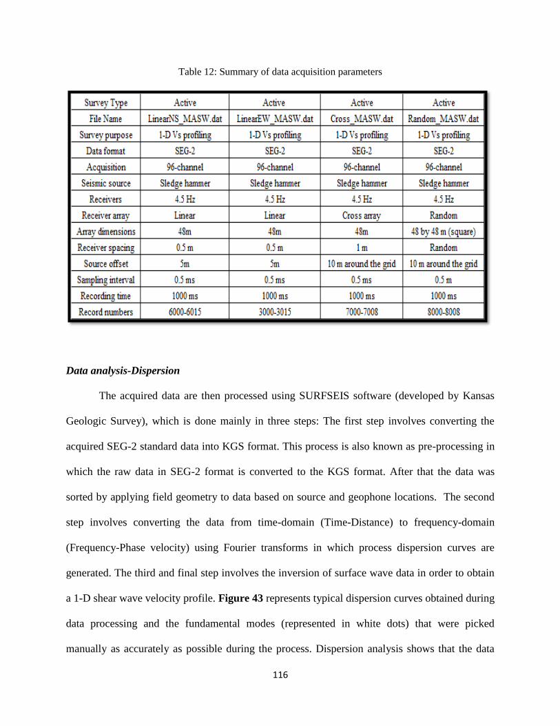
116
Table 12: Summary of data acquisition parameters
Data analysis-Dispersion
The acquired data are then processed using SURFSEIS software (developed by Kansas
Geologic Survey), which is done mainly in three steps: The first step involves converting the
acquired SEG-2 standard data into KGS format. This process is also known as pre-processing in
which the raw data in SEG-2 format is converted to the KGS format. After that the data was
sorted by applying field geometry to data based on source and geophone locations. The second
step involves converting the data from time-domain (Time-Distance) to frequency-domain
(Frequency-Phase velocity) using Fourier transforms in which process dispersion curves are
generated. The third and final step involves the inversion of surface wave data in order to obtain
a 1-D shear wave velocity profile. Figure 43 represents typical dispersion curves obtained during
data processing and the fundamental modes (represented in white dots) that were picked
manually as accurately as possible during the process. Dispersion analysis shows that the data

117
posses dominant frequencies at approximately 15-90 Hz with 0.5 Hz increment and dominant
phase velocities at approximately 100-3000 m/s with 10 m/s increment. Figure 44 represents a
graph comparing dispersion curves for different array types. It is observed from the graph how
well the dispersion curves correlate with one another, especially at higher frequencies (25-90
Hz).
Data Analysis-Inversion
In the final step of data processing, the dispersion curves are inverted to obtain 1-D shear wave
velocity profiles (Figure 45). The profiles are calculated using an iterative inversion process
requiring the dispersion data as input. The process is automated by using least-squares approach
(Xia et al., 1999). In this iteration process, parameters such as Poisson’s ratio, density, and
thickness of the model are kept constant but only Vs is updated after each iteration. These
velocities versus depth profiles generally produce a profile column consisting of ten distinct
velocity layers for the site. Figure 46 is a graph representing shear wave velocities versus depth
comparisons for each array type. It is observed that there is a good correlation between Vs values
for the array types. The velocities thus obtained are further used to interpret the subsurface
geology structure.

118
Figure 43. Dispersion images obtained from shot gathers for various receiver arrays in Figure 34. The X-
axis represents the frequency (Hz) and Y-axis represents the phase velocity (m/s). The white dots on the
dispersion image represent the fundamental mode picks for various receiver arrays.
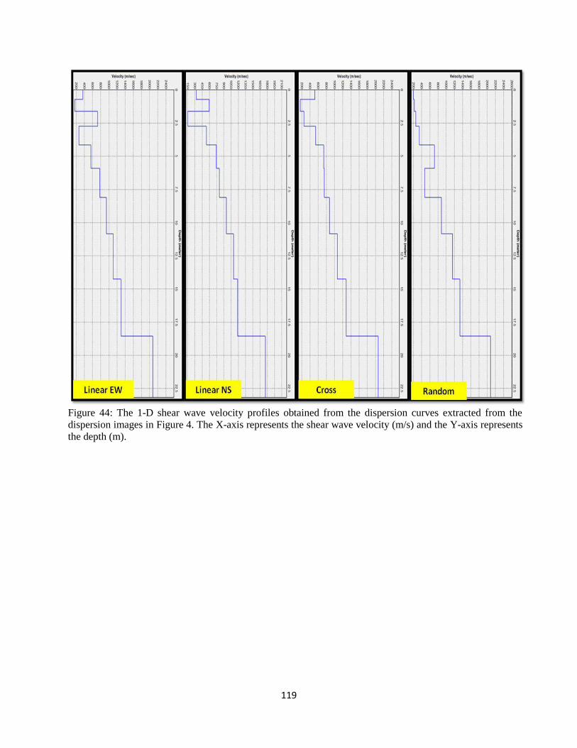
119
Figure 44: The 1-D shear wave velocity profiles obtained from the dispersion curves extracted from the
dispersion images in Figure 4. The X-axis represents the shear wave velocity (m/s) and the Y-axis represents
the depth (m).

120
Figure 45: A graph comparing dispersion curves for various receiver arrays. The X-axis represents
frequency (Hz) and Y-axis represents phase velocity (m/s).

121
Figure 46: Velocity (m/s) versus depth (m) a comparison for various receiver arrays. The X-axis
represents shear wave velocity (m/s) and Y-axis represents depth (m).
Data Interpretation
The shear wave velocities along each survey line for each type of array are evaluated
based on dispersion picks shown in Figure 5. A regolith profile is created describing each layer
(for upper 20m) based on shear wave velocity for each layers. Figure 46 shows that on an
average the shear wave velocities varies from 200 m/s to 2000 m/s for a linear array, 500 m/s to
2000 m/s for cross array, and 400 m/s to 2000 m/s for random array for up to a depth of 20m
from ground level. It is observed from the obtained Vs values that there is a significant variation
in regolith types from ground level to 20m deep. And it is also apparent from the dispersion

122
images that regolith thickness changes significantly even within a relatively narrow area. Since
the dispersion image of the fundamental mode looks different in all kinds of arrays it may be
inferred that the regolith thickness below each array type may be different.
The top layer consists of very stiff regolith having a velocity range of 250 m/s from 0 to 4
m deep. The geologic map of Arizona identifies this material to be Holocene to middle Pliocene
basaltic rocks. Primary rock type found here is alkaline basalt that is mostly dark-colored basaltic
lava and cinders young enough that some original volcanic landforms are still apparent. It
includes basalt as the secondary rock type along with small amounts of andesite, dacite, and
rhyolite. A layer of very dense regolith with a velocity of 700m/s is found to be the second layer
which extends up to a depth of 6m. The third layer is interpreted to be rocky material having a
velocity ranging around 1000 m/s found at a depth ranging from 6 to 8 m. It is also observed that
in this particular location, the hard rock (Vs > 2000 m/s) is found starting at a depth of 8 m and
extending all the way up to 20 m. I interpreted this range to be the approximate depth to bedrock
in that area.
Although more information from geotechnical borings are needed to better constrain the
geologic units at various depths and also depth to bedrock, the estimated depth to bedrock map
published by Arizona Geological Survey suggests that the approximate depth to bedrock at this
site ranges anywhere between 5-15 m. The geologic unit associated with the bedrock at this site
is the tertiary volcanic and sedimentary rocks.
The dynamic properties like the shear modulus and Poisson’s ratio for the linear and
random receiver arrays were calculated based on the shear wave velocity profiles and are
tabulated in Table 15. From Table 3, it is observed that the shear modulus varies from 137 MN/
m2 to 12800 MN/m
2 for linear array, and from 86 MN/ m
2 to 13000 MN/ m
2 for random. It is
123
once again observed here of how well these values correlate with each other for the conventional
linear and newly developed random arrays.
6.5 STATISTICAL ANALYSIS
In order to further compare the datasets obtained from different arrays in more
quantitative way, mixed model approach was performed on all four data sets for inversion data
using SAS programming tool. The results showing significance levels for various models and the
interaction between different geophone patterns with different variables (for example; depth vs.
shear-wave velocity) are tabulated in Tables 13 (a), (b), and (c).
Table 13 (a) shows the significance levels and error terms associated with the assumed model.
The main effects and interactions of different patterns and depth, which were both considered as
fixed factors here, were tested within each block and the output is attached in the Appendix.
Multiple comparisons were run for depth and pattern, as well as their interaction so we can find
the pattern effect in each condition of depth and vice versa. In the table, pattern represents the
geophone arrangement (linear, circular, cross, and random). The replication effect was first
included in the analysis as a factor but since it showed no significant difference at p < 0.05
confidence level, it was removed and the model was re run without rep specified. Table 13 (b)
represents that there is no significant affect of pattern, and pattern * depth with respect to the Vs.
Table 13 (c) tabulates the least-square mean values for effect of depth and Figure 47 shows a
graphical representation of the same. It can be clearly observed from this table of which depth
shows significant differences.

124
It is clearly observed from the ANOVA analysis that there is no significant effect of
pattern or pattern * depth at the p < 0.05 probability level. Since the overall effect of pattern is
not significant there is no need to compare individual patterns with each other in this case.
Table 13: Statistical (mixed model) analysis performed on inversion data using SAS
programming with dependent variable Vs (shear-wave velocity).
(a)
(b)
(c)

125
Figure 47: Least-square means for depth as calculated from mixed model
analysis for the inversion data.
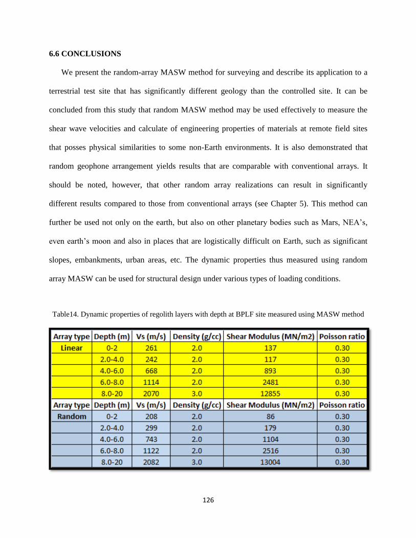
126
6.6 CONCLUSIONS
We present the random-array MASW method for surveying and describe its application to a
terrestrial test site that has significantly different geology than the controlled site. It can be
concluded from this study that random MASW method may be used effectively to measure the
shear wave velocities and calculate of engineering properties of materials at remote field sites
that posses physical similarities to some non-Earth environments. It is also demonstrated that
random geophone arrangement yields results that are comparable with conventional arrays. It
should be noted, however, that other random array realizations can result in significantly
different results compared to those from conventional arrays (see Chapter 5). This method can
further be used not only on the earth, but also on other planetary bodies such as Mars, NEA’s,
even earth’s moon and also in places that are logistically difficult on Earth, such as significant
slopes, embankments, urban areas, etc. The dynamic properties thus measured using random
array MASW can be used for structural design under various types of loading conditions.
Table14. Dynamic properties of regolith layers with depth at BPLF site measured using MASW method
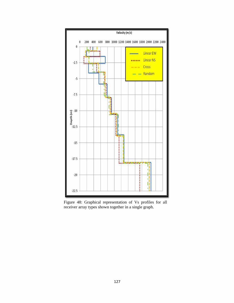
127
Figure 48: Graphical representation of Vs profiles for all
receiver array types shown together in a single graph.

128
Figure 49. Interpreted regolith profile as estimated for the
conventional linear array and newly developed random array
for up to 20 m depth.

129
Chapter 7
Summary, Conclusions and Future Work

130
7.1 SUMMARY AND CONCLUSIONS
This dissertation research introduces a new technique of using random arrangement of
geophones instead of conventional arrays to delineate geotechnical properties within the upper
30 m of the subsurface using Multichannel Analysis of Surface Wave (MASW) technique. Such
kind of arrangement (likely deployed from a mortar-type device) instead of a conventional linear
array is found to be necessary not only for areas that are inaccessible for example, embankments,
urban areas, battle fields, etc. but also for future off-Earth exploration because of the logistical
constraints involved in deploying a linear or circular array robotically or by astronaut. The main
underlying concept behind this study is to improve and increase the usability of the MASW
method by introducing random geophone arrangement to delineate rock and regolith properties.
The MASW method when used along with random geophone arrangement will provide more
readily deployable data acquisition system and this type of information will not only help the
geotechnical community but also other scientific community.
The dissertation contains several individual studies that are all intertwined by a common
application of random geophone array to determine subsurface variations in physical properties
that is hypothesized will be critical for future explorations as they characterize the mechanical
behavior of geotechnical materials under various types of loading. The introductory chapter
includes a brief theory of Rayleigh wave dispersion in heterogeneous media followed by some
basics of MASW method. Followed by the introductory chapter, the third chapter introduces the
random array concept for delineating subsurface properties within the upper 30 m. The fourth
chapter then covers some modeling experiments conducted to determine some key acquisition
parameters pertaining to random array MASW survey. The fifth chapter covers the comparison
of the newly developed array with that of the conventional arrays to determine the accuracy of
131
the random array. Finally, the sixth chapter covers the application of random array MASW
method in determining dynamic properties of subsurface within the upper 30m at a terrestrial
analog environment. Some of the preliminary results and conclusions of the four chapters are
briefly summarized, and the overall impact and overarching implications of this research are
presented.
7.1.1 Random Array Analysis
A new configuration of randomly-distributed receivers for estimating the S-wave velocity
profile of subsurface regolith was introduced. The experiment was performed by collecting
active surface wave data at the University of Tennessee agricultural experimental field site, using
random geophone arrangement. A total of 13 shot points were deployed while collecting the
random data and the shot gather obtained for each shot point location was processed to study the
azimuthal variations in the subsurface. The acquired data has been processed using SURFSEIS
software, for dispersion curve extraction. The dispersion results obtained thus were compared to
conventional linear array data that was acquired at the same location as the random data. The
comparison indicates that the random array correlates fairly well with that of the linear array data
although there is some differences observed. Some variations pertaining to the dispersion data
were observed in the random data that could be due to azimuthal variations in the subsurface.
Statistical analyses were performed on the data to study the variability in the range of velocity
values within the grid. It was concluded that the variations in the velocity values may be due to
the variations in the lithology of the subsurface. It is thus concluded from this study that random
array MASW method can be used to obtain reliable dispersion images and thus 1-D shear wave
velocity profiles that are comparable to conventional linear array and it can further be used to
map subsurface geology to an acceptable level.
132
7.1.2 Forward-Modeling Experiments
Influence of random geophone array on the resolution of dispersion curve using forward
modeling method in multichannel analysis of surface wave (MASW) surveys is described here
on a theoretical perspective of the dispersion curve imaging method used during a normal
implementation of MASW method. Parameters like clustered geophones, skewness of receivers,
different receiver numbers, total number of traces and their influence on dispersion image are
described in this study. It was concluded based on the modeling results that in order to obtain
best dispersion data from a random array MASW survey the geophones a) should be as
dispersive (less clustered) as possible, b) should be normally skewed around the grid (although
right or left skewed data also yield reliable dispersion images, a normally skewed data yields
high λmax, which in turn gives more depth of penetration, and c) A higher number of traces
results in high resolution dispersion image, however it is only necessary to increase the number
of traces only if you are increasing the area of coverage.
7.1.3 Comparison of Various Geophone Arrays
This study is mainly performed to compare the newly developed random array with four
different types of MASW geophone arrays (Linear EW, Linear NS, cross and circular). For this,
more active surface wave data were collected at the same site and location using different array
configurations. All the data thus acquired were processed using SURFSEIS software and
dispersion curves were extracted for each array type. The dispersion picks were further inverted
to obtain 1-D shear wave velocity profiles which were used for comparison. It was observed that
the more dispersive the geophones are in a random array, the better the resolution of the
dispersion image, and thus the 1-D Vs interpretations. To statistically evaluate the random array

133
data, four different random sets were collected each with different X and Y coordinates and some
of the random array Vs profiles were significantly different from the conventional Vs profiles at
certain depths. Therefore, it can be concluded from this study that care needs to be taken in
interpreting the results from random arrangements of geophones since results from one random
array can differ significantly from those for another random array or conventional pattern.
7.1.4 Application of Random Array MASW
This study presents the MASW method, surveying and its application to a site whose
geology is very different than that of the controlled site used in the study. While the controlled
site is mainly a flood plain with more consolidated material, the BPLF site represents a 2 million
year old lava deposits and the site is filled with unconsolidated basaltic rocks. To achieve this
goal, MASW data was collected at the Black Point Lava flow site (BPLF), Flagstaff, Arizona.
The data was collected for four different geophone arrays (linear EW, Linear NS, cross, and
random). The data was processed for dispersion curves which were in turn used to obtain the
shear wave velocity profiles of the subsurface. The dynamic properties like the shear modulus
and Poisson’s ratio were calculated based on the shear wave velocity profiles for linear and
random arrays and it was observed that the values correlated very well for the conventional
linear and newly developed random array. However, the random MASW method cannot be used
to routinely measure shear wave velocities and calculate dynamic properties of materials on
terrestrial analog environments, because the results vary with each different realization of the
random array setup.

134
7.2 OVERALL CONCLUSIONS AND IMPLICATION OF RESEARCH
The overall theme of the research presented herein is that systematic use of random array
MASW method is a viable technique for determining engineering properties of the subsurface
within the upper 30 m. Although conventional array types have proven adept for delineating
regolith properties, the type of array that you choose is at least partially controlled by the site
viability and other conditions. Thus, in some hard-to-reach places like the battlefields,
embankments, urbanized locations or even any other kind of planetary surfaces such as Mars
etc., where there might be places that can be unreachable or it is simply not possible to arrange a
systematic linear or circular array robotically (or by an astronaut) on the surface due to logistical
reasons, a randomly distributed geophone array (likely to be deployed using a mortar-type
device) will be most useful. Additionally there is information that can be obtained from random
array like the azimuthal variations in the subsurface that are likewise difficult to determine using
other geophone arrangements.
The random array MASW method is a novel approach. The geotechnical properties obtained
from this new technique although applicable on Earth are also intended for surfaces and regolith
in the future exploration of planetary bodies for possible human habitation. This would include
Mars, its Moon-Phobus/Deimos, Near-Earth Asteroids (NEA’s), even Earth’s Moon. With each
situation, the nature of the regolith and its formational processes will place certain restrictions
and limitations upon the applications. This is expected with any change of terrains even on the
Earth, let alone between planetary bodies. It should also be noted, however, that other random
array realizations can result in significantly different results compared to those from
conventional arrays. Therefore care should be taken while deploying a random array and various
135
different aspects such as skewness, clusteredness, etc. should be considered while performing
random array MASW survey.
7.3 FUTURE WORK
There are a number of additional investigative components—not conducted within the scope
of this project—which could be expanded for future projects.
1. Further evaluation of random array can be performed in terms of dispersion curve
analysis. Data can be collected with much larger grid dimensions using more number of
geophones (of lower frequency) to see if we can obtain much deeper depth information. Also
analysis of errors associated with dispersion picks or any other kind of computational
artifacts during data acquisition or processing stage can be further evaluated by collecting
more number of random arrays. Collecting random array data using passive sources (like
traffic noise or wind) and then combining both active and passive data might result in much
better dispersion analysis as in theory active data provides information at higher frequencies
and passive data covers the lower part of frequencies in a dispersion image. Therefore
looking at combined results would provide us more information about subsurface features.
2. Based on the modeling results effort can be made to collect real field data in order to
study the effect of clustered array, skewness effect etc. Also further models can be generated
to study the effect of passive source on random array data, or to analyze more on other offset
related parameters like source-offset distance, receiver spacing, total length of the array, etc.
3. Apply the newly developed methodology to additional terrestrial analog sites and in other
inaccessible areas like urban areas where in it is difficult to deploy a linear or circular array
for further refining the methodology proposed in this research. And hopefully, this method
can be applied on the moon and other planetary bodies during future missions.

136
REFERENCES

137
Abo-Zena, A.M. (1979). “Dispersion function computations for unlimited frequency values.”
Geophys. J. R. Astr. Soc., 58, 91-105.
Achenbach, J.D. (1973). Wave propagation in elastic solids, North-Holland, 425p.
Aki, K. (1965). A note on the use of microseismics in determining the shallow structures of the
Earth’s crust: Geophysics, Vol 30, 665-666
Aki, K., and Richards, P.G. (1980). Quantitative Seismology-Theory and Methods, Vol.1 and 2,
Freeman Company, San Fransisco, 932p.
Aki, K., and Richards, P.G., 1980, Quantitative seismology:W.H. Freeman & Co. Mari, J. L.,
1984, Estimation of static correction for shear-wave profilingusing the dispersion
properties of Love waves: Geophysics, 49, 1169–1179.
Al-Hunaidi, M.O., and Rainer, J.H., 1995, Analysis of multi-mode signals of the SASW method,
Proc 7th Int. Conf. Regolith Dynamics and Earthquake Eng., p. 259-266.
Aouad, M.F., 1993, Evaluation of Flexible Pavements and Subgrades Using the Spectral-
Analysis-of-Surface-Waves (SASW) Method, PhD thesis, Univ. of Texas at
Austin, Texas.
About Analog Missions and Filed Tests. (2011). Retrieved June 11, 2012, from
http://www.nasa.gov/exploration/analogs/about.html .
About NASA Desert-RATS program (news and features blog). (2012). Retrieved on June 11,
2012, from http://www.nasa.gov/exploration/analogs/desert_rats.html.
Arizona’s Black Point Lava Flow Beckons NASA’s Desert Rats. (2010). Retrieved on August
24, 2010, from http://spacecoalition.com/uncategorized/arizonas-black-point-lava-flow-
beckons-nasas-desert-rats?doing_wp_cron.
Babuska, V., and Cara, M., (1991). Seismic anisotropy in the earth: Kluwer Academic
Publishers.
Baker, G.S., Steeples, D.W., Schmeisner, C., 1999. In situ, high-resolution P-wave velocity
measurements within 1 m of the Earth’s surface: Geophysics, 64, no 2, 323-325
Baker, G.S., Steeples, D.W., Schmeissner, C., and Spikes, K.T., 2000, Source-dependent
frequency content of ultrashallow seismic reflection data: Bull. Seis. Soc. Amer., 90, 2,
494-499
Baker, G.S., Steeples, D.W., and Schmeissner, C, 2002, The effect of seasonal regolith-moisture
conditions on near-surface seismic reflection data quality: First Break, 20, no 1, 35-41
138
Baker, G.S., Strasser, J.C., Evenson, E.B., Lawson, D.E., Pyke, K.P., and Bigl, R.A., 2003, Near
surface seismic reflection profiling of the Matanuska Glacier,
Alaska USA: Geophysics, 68, no 1, 147-156
Bates R. L. and Jackson J. A., eds. (1980) The Glossary of Geology, 2nd
Edition. American
Geological Institute, Washington. 751 pp.
Bekker M. G. (1969) Introduction to Terrain—Vehicle Systems. Univ. of Michigan, Ann Arbor.
Bishop A. W. (1955) The use of the slip circle in the stability analysis of earth slopes.
Geotechnique, 5, 7–17.
Bolt, B.A. (1993). Earthquakes, W.H.Freeman, New York, 331p.
Bullen, K.E. (1963). An introduction to the theory of Seismology: Cambridge Univ. Press.
Black Point Lava Flow, Arizona (Image). (2009). Retrieved on September 7, 2009, from
http://earthobservatory.nasa.gov/IOTD/view.php?id=40076 .
Cadigan, R.A, 1962, A method for determining the randomness of regionally distributed
quantitative geologic data: Journal of sedimentary Petrology, 32, 813-818.
Dobrin, M.B., Savit, C.H. (1988). Introduction to Geophysical Prospecting.
Dorman, J., and Ewing, M., 1962, Numerical inversion of seismic surface wave dispersion data
and crust-mantle structure in the New York–Pennsylvania area: J. Geophys. Res., 67,
5227, 5241.
Ewing, W. M., Jardetzky, W. S., and Press, F. (1957). Elastic waves in layered media McGraw-
Hill, New York. 380p.
Folk R. L. (1968) Petrology of Sedimentary Rocks. Hemphill’s, Austin. 170 pp.
Fonquinos Mera, R., 1995, Dynamic nondestructive testing of pavements, PhD thesis, Univ. of
Texas at Austin, Texas.
Foti, S., 2000, Multistation methods for geotechnical characterization using surface waves: PhD
thesis, Politecnico di Torino, Italy.
Gabriels, P., Snider, R., and Nolet, G., 1987, In situ measurements of shear-wave velocity in
sediments with higher-mode Rayleigh waves: Geophys. Prospecting, 35, 187-196.
Ganji, V., Gucunski, N., and Nazarian, S., 1998, Automated inversion procedure for spectral
analysis of surface waves, J. Geotech. Engrg., ASCE, v. 124, n. 8, p. 757-770.
Graff, K.F. (1975). Wave motion in elastic solids, Dover Publications, New York, 649p.

139
Gucunski, N., and Woods, R.D., 1992, Numerical simulation of the SASW test, Regolith Dyn
and Earth-quake Engrg. J., v. 11, n. 4, p. 213-227.
Haskell, N. A. 1953, The dispersion of surface waves on multilayered media, Bull. Seismological
Soc. of Am., v. 43, n. 1, p. 17-34.
Haskell, N.A. (1953). “The dispersion of surface waves in multilayered media.’ Bulletin of the
Seismological Society of America,43, 17-34.
Heisey, J.S., Stokoe II, K.H., and Meyer, A.H., 1982, Moduli of pavement systems from Spectral
Analysis of Surface Waves, Transp. Res. Rec., v. 852, Washington D.C, p. 22-31.
Hilterman, F, 1990, Is AVO the seismic signature of lithology? A case history of ship Shoal
South Addition: The Leading Edge, 9(6), 15-22.
Hiltunen, D.R., and Gucunski, N., 1994, Annotated bibliography on SASW, in Geophysical
character-ization of sites, ISSMFE Technical Committee #10, edited by R.D. Woods,
Oxford Publishers, New Delhi.
Hisada, Y. (1994). “An efficient method for computing Green’s functions for a layered half-
space with sources and receivers at close depths.” Bulletin of the Seismological Society of
America, 84(5), 1456-1472.
Hisada, Y. (1995). “An efficient method for computing Green’s functions for a layered half-
space with sources and receivers at close depths (Part 2).” Bulletin of the Seismological
Society of America, 85(4), 1080-1093.
Ivanov, J., Park, C.B., Miller, R.D., and Xia, J., 2000a, Mapping Poisson’s Ratio of
unconsolidated materials from a joint analysis of surface-wave and refraction events:
Proceedings of the Symposium on the Application of Geophysics to Engineering and
Environmental Problems, Arlington, Va.,February 20-24, 2000
Jones, R., 1955, A vibration method for measuring the thickness of concrete road slabs in situ,
Magazine of Concrete Research, v. 7, n. 20, p. 97-102.
Jones, R., 1962, Surface wave technique for measuring the elastic properties and thickness of
roads: Theoretical development, British Journal of Applied Physics, v.13, p. 21-29.
Jones, R.B. (1958). “In-situ measurement of the dynamic properties of regolith by vibration
methods.” Geotechnique, 8(1), 1-21.
Joel, S.W., (1966): Investigation of in situ Physical Properties of Surface and Subsurface Site
Materials by Engineering Geophysical Techniques, Annual Report, Retrieved on July 22,
2011,from
http://ntrs.nasa.gov/archive/nasa/casi.ntrs.nasa.gov/19660028076_1966028076.pdf .
140
Kausel, E., and Roesset, J.M., (1981). “Stiffness matrices for layered regoliths.” Bulletin of the
Seismological Society of America, 71(6), 1743-1761.
Kennet, B. L. N. (1974). “Reflections, rays, and reverberations.” Bulletin of the Seismological
Society of America, 64, 1685-1696.
Kennet. B. L. N., and Kerry, N. J. (1979). “Seismic waves in a stratified half space.”
Geophysical J. Royal Astronomical Society, 57, 557-583.
Lai, C.G. (1998). Simultaneous inversion of Rayleigh phase velocity and attenuation for near-
surface site characterization, PhD dissertation, Georgia Institute of Technology, 370p.
Martinez, J., Ortega, A.A., and McMechan, G.A., 2000, 3-D seismic modeling for cracked
media: shear-wave splitting at zero offset, Geophysics, 65, 211-221.
Maxwell D. E. (1977) Simple Z model of cratering, ejection and the overturned flap. In Impact
and Explosion Cratering (D. J. Roddy, R. O. Pepin, and R. B. Merrill, eds.), pp. 1003–
1008. Pergamon, New York.
Mckay D.S., Fruland .M., and Heiken G.H.(1974) Grain size and evolution of planetary
regoliths. Proc. Planetary Sci. Conf. 5th
, pp. 887-906.
Mckay D.S., Heiken G.H., Basu A., Blanford G., Simon S., Reedy R., French B.M., and Papike
J. (1991). The planetary regolith. In: Heiken, G., Vaniman D., French, B. (Eds.),
Planetary Sourcebook, a user’s guide to the moon. New York: Cambridge University
Press. P.736.
McMechan, G. A., and Yedlin, M. J., 1981, Analysis of dispersive waves by wave field
transformation: Geophysics, 46, 869-874.
Miller, R.D., Xia, J., Park, C.B., and Ivanov, J., 1999, Multichannel analysis of surface waves to
map bedrock, The Leading Edge, 18, no. 12, 1392-1396.
Miller, R.D., Xia, J., Park, C.B., and Ivanov, J., 1999, Multichannel analysis of surface waves to
map bedrock, The Leading Edge, 18, no. 12, 1392-1396.
Multichannel Analysis of Surface Waves (MASW). (2007). Retrived on May 2009 from
http://www.masw.com/index.html.
Nakamura, Y., Lammelein, D., Latham, G., Ewing, M., Dorman, J., Press, F and Toksoz, N
(1973): New seismic data on the state of the deep planetary interior, Science, Vol 181,
No. 4094, 49 51.
Nakamura, Y., Lammlein, D., Latham, G., Ewing, M., Dorman, J., Press, F., and Toksoz, N.,
1973, New Seismic Data on the State of the Deep Planetary Interior: Science, 181, 49-51.
141
Nazararian, S., Stokoe II, K.H., and Hudson, W.R., 1983, Use of spectral analysis of surface
waves method for determination of moduli and thickness of pavement systems:
Transportation Research Record No. 930, 38-45.
Nazararian, S., Stokoe II, K.H., and Hudson, W.R., 1983, Use of spectral analysis of surface
waves method for determination of moduli and thickness of pavement systems:
Transportation Research Record No. 930, 38-45.
Nazarian, S. (1984). Insitu determination of elastic moduli of regolith deposits and pavement
systems by Spectral-Analysis-of-Surface-Waves method, PhD dissertation, Uni. Of Texas
of Austin. Okada, H. (2003). The microtremor survey method, SEG, 135p.
Nazarian, S., Stokoe II, K.H., and Hudson, W.R. (1983): Use of spectral analysis of surface
waves method for determination of moduli and thickness of pavement systems:
Transportation Research Record No.930, 38-45.
O’Neill, A., 2003, Full-waveform reflectivity for modeling, inversion and appraisal of seismic
surface wave dispersion in shallow site investigations, Ph.D. thesis, The University of
Western Australia, Australia.
Park, C. B., Ivanov, J., Miller, R. D., Xia, J., and Ryden, N., 2001a, Multichannel analysis of
surface waves (MASW) for pavement: Feasibility test: 5th SEGJ Int. Symposium, Tokyo,
Japan, January 24-26, 2001.
Park, C.B., Miller, R.D., and N.Ryden, 2006, Roadside seismic survey utilizing traffic noise:
Proceedings of the NDE conference on Civil Engineering, St. Louis. MO, August 14-18,
317-324.
Park, C.B., Miller, R.D., and Xia, J., 1998, Ground roll as a tool to image near-surface anomaly:
[Expanded Abstract]: Soc. Explor. Geophys. 874-877.
Park, C.B., Miller, R.D., and Xia, J., 1998, Imaging dispersion curves of surface waves on multi
channel record: [Expanded Abstract]: Soc. Explor. Geophys., 1377-1380.
Park, C.B., Miller, R.D., and Xia, J., 1999, Multi-channel analysis of surface waves (MASW):
Geophysics, v. 64, no. 3, p. 800-808.
Park, C.B., Miller, R.D., and Xia, J., 2001, Offset and resolution of dispersion curve in
multichannel analysis of surface waves (MASW): Proceedings of the SAGEEP 2001,
Denver, Colorado, SSM4.
Park, C.B., Miller, R.D., N.Ryden., Xia,J., and Ivanov, J. 2005: Combined use of active and
passive surface waves: Journal of Environmental & Engineering Geophysics, Vol 10,
No.3, 323 334.
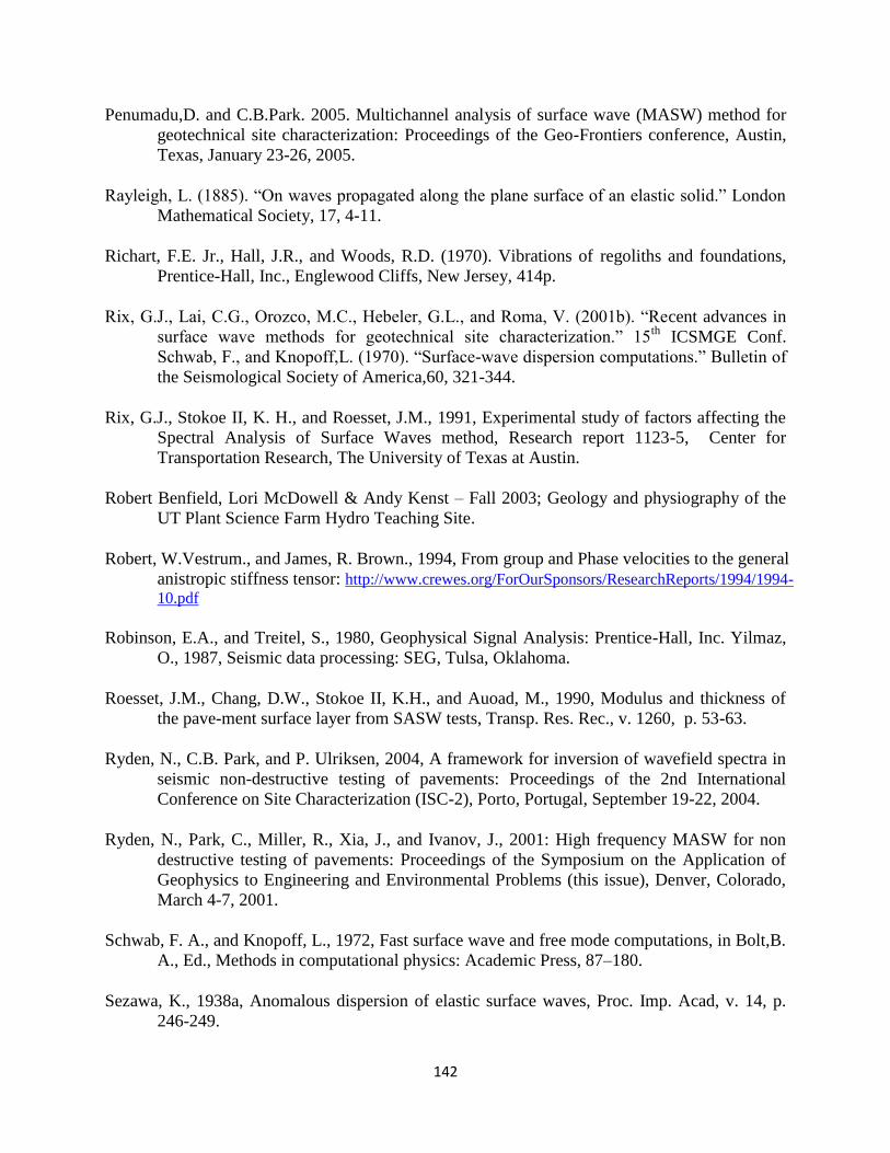
142
Penumadu,D. and C.B.Park. 2005. Multichannel analysis of surface wave (MASW) method for
geotechnical site characterization: Proceedings of the Geo-Frontiers conference, Austin,
Texas, January 23-26, 2005.
Rayleigh, L. (1885). “On waves propagated along the plane surface of an elastic solid.” London
Mathematical Society, 17, 4-11.
Richart, F.E. Jr., Hall, J.R., and Woods, R.D. (1970). Vibrations of regoliths and foundations,
Prentice-Hall, Inc., Englewood Cliffs, New Jersey, 414p.
Rix, G.J., Lai, C.G., Orozco, M.C., Hebeler, G.L., and Roma, V. (2001b). “Recent advances in
surface wave methods for geotechnical site characterization.” 15th
ICSMGE Conf.
Schwab, F., and Knopoff,L. (1970). “Surface-wave dispersion computations.” Bulletin of
the Seismological Society of America,60, 321-344.
Rix, G.J., Stokoe II, K. H., and Roesset, J.M., 1991, Experimental study of factors affecting the
Spectral Analysis of Surface Waves method, Research report 1123-5, Center for
Transportation Research, The University of Texas at Austin.
Robert Benfield, Lori McDowell & Andy Kenst – Fall 2003; Geology and physiography of the
UT Plant Science Farm Hydro Teaching Site.
Robert, W.Vestrum., and James, R. Brown., 1994, From group and Phase velocities to the general
anistropic stiffness tensor: http://www.crewes.org/ForOurSponsors/ResearchReports/1994/1994-
10.pdf
Robinson, E.A., and Treitel, S., 1980, Geophysical Signal Analysis: Prentice-Hall, Inc. Yilmaz,
O., 1987, Seismic data processing: SEG, Tulsa, Oklahoma.
Roesset, J.M., Chang, D.W., Stokoe II, K.H., and Auoad, M., 1990, Modulus and thickness of
the pave-ment surface layer from SASW tests, Transp. Res. Rec., v. 1260, p. 53-63.
Ryden, N., C.B. Park, and P. Ulriksen, 2004, A framework for inversion of wavefield spectra in
seismic non-destructive testing of pavements: Proceedings of the 2nd International
Conference on Site Characterization (ISC-2), Porto, Portugal, September 19-22, 2004.
Ryden, N., Park, C., Miller, R., Xia, J., and Ivanov, J., 2001: High frequency MASW for non
destructive testing of pavements: Proceedings of the Symposium on the Application of
Geophysics to Engineering and Environmental Problems (this issue), Denver, Colorado,
March 4-7, 2001.
Schwab, F. A., and Knopoff, L., 1972, Fast surface wave and free mode computations, in Bolt,B.
A., Ed., Methods in computational physics: Academic Press, 87–180.
Sezawa, K., 1938a, Anomalous dispersion of elastic surface waves, Proc. Imp. Acad, v. 14, p.
246-249.
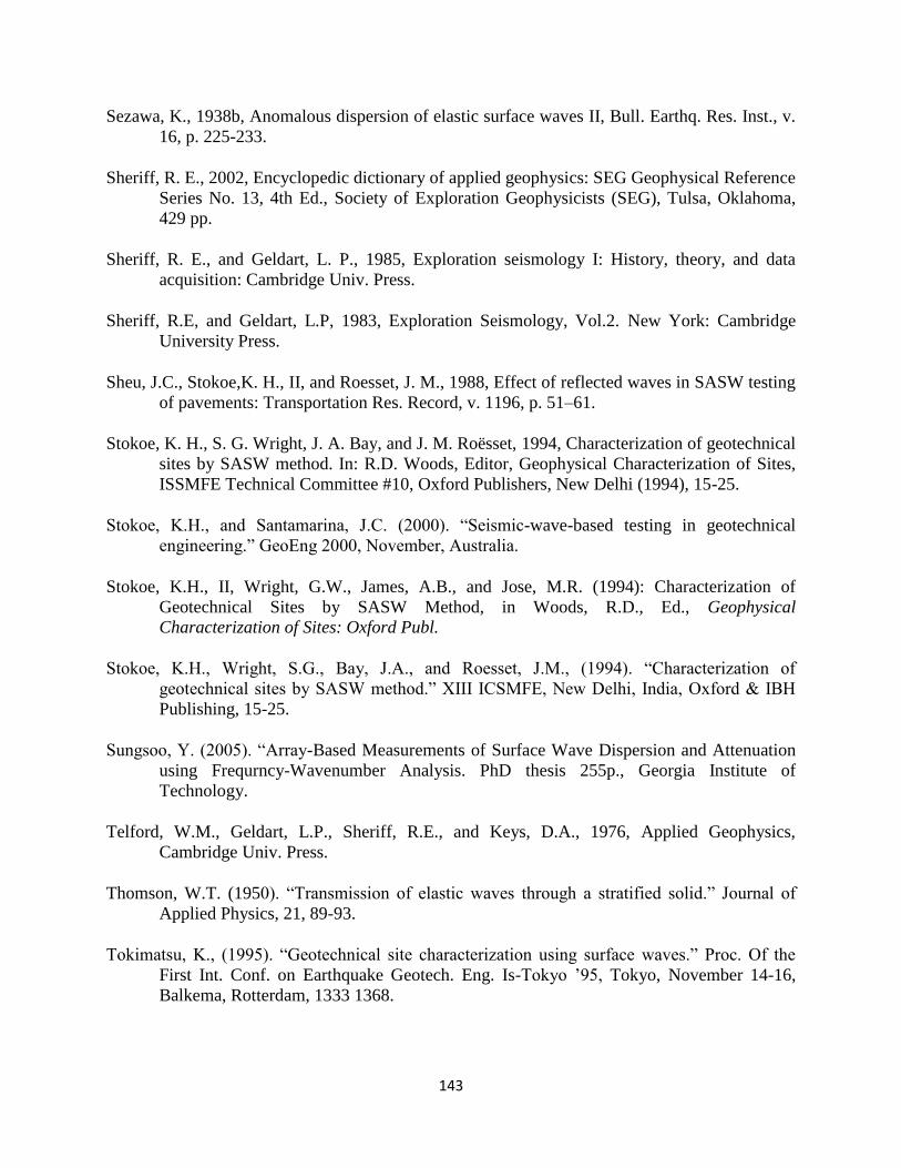
143
Sezawa, K., 1938b, Anomalous dispersion of elastic surface waves II, Bull. Earthq. Res. Inst., v.
16, p. 225-233.
Sheriff, R. E., 2002, Encyclopedic dictionary of applied geophysics: SEG Geophysical Reference
Series No. 13, 4th Ed., Society of Exploration Geophysicists (SEG), Tulsa, Oklahoma,
429 pp.
Sheriff, R. E., and Geldart, L. P., 1985, Exploration seismology I: History, theory, and data
acquisition: Cambridge Univ. Press.
Sheriff, R.E, and Geldart, L.P, 1983, Exploration Seismology, Vol.2. New York: Cambridge
University Press.
Sheu, J.C., Stokoe,K. H., II, and Roesset, J. M., 1988, Effect of reflected waves in SASW testing
of pavements: Transportation Res. Record, v. 1196, p. 51–61.
Stokoe, K. H., S. G. Wright, J. A. Bay, and J. M. Roësset, 1994, Characterization of geotechnical
sites by SASW method. In: R.D. Woods, Editor, Geophysical Characterization of Sites,
ISSMFE Technical Committee #10, Oxford Publishers, New Delhi (1994), 15-25.
Stokoe, K.H., and Santamarina, J.C. (2000). “Seismic-wave-based testing in geotechnical
engineering.” GeoEng 2000, November, Australia.
Stokoe, K.H., II, Wright, G.W., James, A.B., and Jose, M.R. (1994): Characterization of
Geotechnical Sites by SASW Method, in Woods, R.D., Ed., Geophysical
Characterization of Sites: Oxford Publ.
Stokoe, K.H., Wright, S.G., Bay, J.A., and Roesset, J.M., (1994). “Characterization of
geotechnical sites by SASW method.” XIII ICSMFE, New Delhi, India, Oxford & IBH
Publishing, 15-25.
Sungsoo, Y. (2005). “Array-Based Measurements of Surface Wave Dispersion and Attenuation
using Frequrncy-Wavenumber Analysis. PhD thesis 255p., Georgia Institute of
Technology.
Telford, W.M., Geldart, L.P., Sheriff, R.E., and Keys, D.A., 1976, Applied Geophysics,
Cambridge Univ. Press.
Thomson, W.T. (1950). “Transmission of elastic waves through a stratified solid.” Journal of
Applied Physics, 21, 89-93.
Tokimatsu, K., (1995). “Geotechnical site characterization using surface waves.” Proc. Of the
First Int. Conf. on Earthquake Geotech. Eng. Is-Tokyo ’95, Tokyo, November 14-16,
Balkema, Rotterdam, 1333 1368.

144
Tokimatsu, K., Tamura, S., and Kojima, H., 1992, Effects of multiple modes on Rayleigh wave
dispersion characteristics, J. Geotech. Engrg., ASCE, v. 118, n. 10, p.1529-1543.
Terrestrial Analogue Sites (Space analogues). (2012). Retrieved on September 24, 2012, from
http://en.wikipedia.org/wiki/Terrestrial_Analogue_Sites .
Van der Pol, C., 1951, Dynamic testing of road constructions, J. appl. Chem., v. 1, July, p. 281-
290.
Vidale, R.F., 1964, The dispersion of stress waves in layered media overlaying a half space of
lesser acoustic rigidity, Ph.D. Thesis, Univ. of Wisconsin.
Viktorov, I.A (1957). Rayleigh and Lamb waves: physical theory and applications, Plenum
Press, New York, 154p.
Watkins, J.S., Walters, L.A., and Godson, R.H., 1972, Dependence of in situ compressional
wave velocity on porosity in unsaturated rocks: Geophysics, 37, 29-35.
Williams, T.P., and Gucunski, N., 1995, Neural networks for backcalculation of moduli from
SASW test, J. Comp. In Civ. Engrg, ASCE, v. 9, n. 1, p. 1-8.
Xia, J., R. D. Miller, and C. B. Park, 1999, Estimation of near-surface S-wave velocity by
inversion of Rayleigh waves: Geophysics 64, 691–700.
Xia, J., R.D. Miller, C.B. Park, and G. Tian, 2003, Inversion of high frequency surface waves
with fundamental and higher modes: Journal of Applied Geophysics, 52, no. 1, 45-57.
Xia, Jhianghai., Xu, Yixian, Miller, R.D., 2007, Generating an image of Dispersive Energy by
Frequency Decomposition and slant Stacking: Pure and Applied Geophysics, 164, 1-16.
Xia, J., Miller, R.D., and Park, C.B., 1999, Estimation of near-surface shear-wave velocity by
inversion of Rayleigh waves: Geophysics, v. 64, no. 3, p. 691-700.
Xia, J., Miller, R.D., and Park, C.B., 2000a, Advantages of calculating shear-wave velocity from
surface waves with higher modes: [Exp.Abs.]: Soc.Expl.Geophys., p., 1295-1298.
Yeluru, P., Baker, G., Park, C.B., and Taylor, L., 2008, New developments in seismic surface
waves data acquisition and processing:Symposium on the Application of Geophysics to
Engineering and Environmental Problems (SAGEEP 2008), Philadelphia, April 6-10,
Proceedings on CD Rom.

145
Appendices

146
APPENDIX A
Overview of Multi-channel Analysis of Surface Wave (MASW) method

147
3.1 INTRODUCTION
As described in Chapter 2, there are two types of surface waves: Rayleigh and Love
waves (Dobrin and Savit, 1988). Both represent the plane-wave solutions to the coupled elastic
wave equation (see Haskell, 1953):
∂2/∂t
2 = Vp
2
2 and ∂
2/∂t
2 = Vs
2
2……(3.1)
In most of near-surface active-source seismic surveys when a compressional source is used, more
than two-thirds of total seismic energy generated is imparted into Rayleigh waves (Richart et al.,
1970), which is the principal component of surface waves generated most effectively in all kinds
of surface seismic surveys. As previously described, surface waves obey the property of
dispersion i.e. for a vertical velocity variation, each frequency component of a surface wave has
a different propagation velocity (also called phase velocity), that in turn results in a different
wavelength for each frequency of the propagated wave. Therefore, due to its dispersive property,
ground roll can be utilized to infer near-surface elastic properties (Nazarian et al., 1983; Stokoe
et al., 1994; Park et al., 1998a).
Constructing shear-wave velocity profiles through the analysis of plane-wave
fundamental mode Rayeligh waves is one of the most common ways to use the dispersive
properties of surface waves (Bullen, 1963). The phase velocities for different wavelengths can be
found from the solutions to the wave equation (as described in Chapter 2) by treating the near
surface materials as layered earth medium (Haskell, 1953). Therefore, by analyzing the
dispersion feature of ground roll represented in recorded seismic data, the near-surface S-wave

148
velocity (Vs) profiles can be constructed and the corresponding shear moduli () are calculated
from the relation between the two parameters.
Vs =(/)1/2
…..(3.2)
where represents the density of material (assumed as constant since it varies little with depth
(as compared to the scale of variations in bulk and shear modulus).
3.2 HISTORICAL CONTEXT OF THE SURFACE-WAVE METHOD
Early pioneering work in surface waves goes back to 1950s when the steady state method
was first used by Van der Pol (1951) and Jones (1955) (Figure A1). Most commonly known as
the Continuous Surface Wave method (Mathew et al., 1996; Figure A2), it is based on the
fundamental-mode (M0) only, and at the time other Rayleigh wave assumptions and all other
types of waves-higher modes, body waves, etc. were all ignored. While this method was gaining
popularity amongst the geotechnical community, Tokimatsu et al. (Year) redefined the soil site
inversion theory. Since the very early stage of the surface wave application, pavement was found
to be more complex than soil (Sezawa, 1938; Press and Dobrin, 1956), with a special type of
guided wave called the “leaky wave” that required a complex-domain approach in solving wave
equations (Jones, 1962; Vidale, 1964). Martincek (1994) introduced a modern computer
approach, but it still produced limited results.

149
Figure A1. Steady state methods from 1950’s. UK 1950s (left) and Van der Pool (1951) (right)
Figure A2. The Continuous Surface Wave method (from Mathew et.al., 1996)

150
3.2.1 Two-Receiver Approach (The SASW Method)
The Spectral Analysis of Surface Waves (SASW) method (Heisey et al., 1982) was
introduced by scientists at University of Texas-Austin in the early 1980’s. This method is based
on the Fast Fourier Transform (FFT) analysis of phase spectra of surface waves generated by
using an impulsive source like the sledge hammer (Figure A3). It was then that this method
became widely used among geotechnical engineers and researchers. During the initial stage,
again only the fundamental-mode (M0) Rayleigh wave assumption was used, but simultaneous
multi-frequency generation from the impact seismic source and then by FFT during the
subsequent data processing stage greatly improved overall efficiency of the method in
comparison to conventional methods such as the continuous surface wave (CSW) method.
Significant research on this method has since been conducted at UT-Austin (Nazarian et al.,
1983; Rix et al., 1991; Al-Hunaidi, 1992; Gucunski and Woods, 1992; Aouad, 1993; Stokoe et
al., 1994; Fonquinos, 1995; Ganji et al., 1998). More detailed information on this method and
more detailed and complete list of publications on SASW up to early 1990’s can be found in
“Annotated bibliography on SASW” by Hiltunen and Gucunski (1994).
During the early stage of use, the SASW method was focused only on ways to enhance
accuracy of the fundamental-mode (M0) Rayleigh-wave dispersion curve through field
procedure and data processing efforts. But soon it was recognized that there might be a
possibility of the curve “being more than M0” and therefore the concept of Higher Modes
(HM’s) were introduced in the studies (Roesset et al., 1990; Rix et al., 1991; Tokimatsu et al.,
1992; Stokoe et al., 1994). It was then that the concept of “apparent (or effective)” dispersion
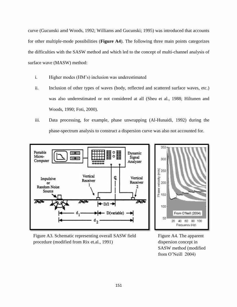
151
curve (Gucunski amd Woods, 1992; Williams and Gucunski; 1995) was introduced that accounts
for other multiple-mode possibilities (Figure A4). The following three main points categorizes
the difficulties with the SASW method and which led to the concept of multi-channel analysis of
surface wave (MASW) method:
i. Higher modes (HM’s) inclusion was underestimated
ii. Inclusion of other types of waves (body, reflected and scattered surface waves, etc.)
was also underestimated or not considered at all (Sheu et al., 1988; Hiltunen and
Woods, 1990; Foti, 2000).
iii. Data processing, for example, phase unwrapping (Al-Hunaidi, 1992) during the
phase-spectrum analysis to construct a dispersion curve was also not accounted for.
Figure A3. Schematic representing overall SASW field
procedure (modified from Rix et.al., 1991)
Figure A4. The apparent
dispersion concept in
SASW method (modified
from O’Neill 2004)
152
3.2.2 The Multi-channel Approach (MASW)
The multi-channel analysis of surface waves method (MASW), first introduced into
geotechnical and geophysical community in early 2000s (Park et al., 1999), is a seismic method
which generates a shear wave velocity profile (i.e., Vs versus depth) by analyzing Rayleigh-type
surface waves on a multi-channel (multiple geophones) record. The project actually started in
mid-90s at the Kansas Geological Survey (KGS) by geophysicists who had been utilizing
seismic reflection method to image earth’s interior for depths up to several kilometers. At that
time, surface waves were considered as a significant source of noise that was to be attenuated
(Figure A5). But later this surface wave method, also called as the high-resolution reflection
method, was used to image very shallow depths of engineering interest (e.g., 100 m or less;
Baker, 1999). Keeping in mind the drawbacks in the SASW method, which clearly reached its
limitation to handle complexities, the MASW method was mainly utilized for the purpose of
geotechnical engineering projects. It is a seismic exploration method evaluating ground stiffness
in 1-D, 2-D and 3-D formats for various types of geotechnical engineering projects. Since first
introduction in the late 1990’s, MASW has been utilized by numerous practitioners and
researched by many investigators worldwide. Based on the theory that the number of geophones
used can directly impact the resolving power of the method, researchers utilized diverse
techniques already available after a long history of seismic data analysis (Telford et al., 1976;
Robinson and Treitel, 1980; Yilmaz, 1987), and also developed new strategies in field and data
processing to detail surface wave propagation properties and characterized key issues to bring
out a routinely-useable seismic method.
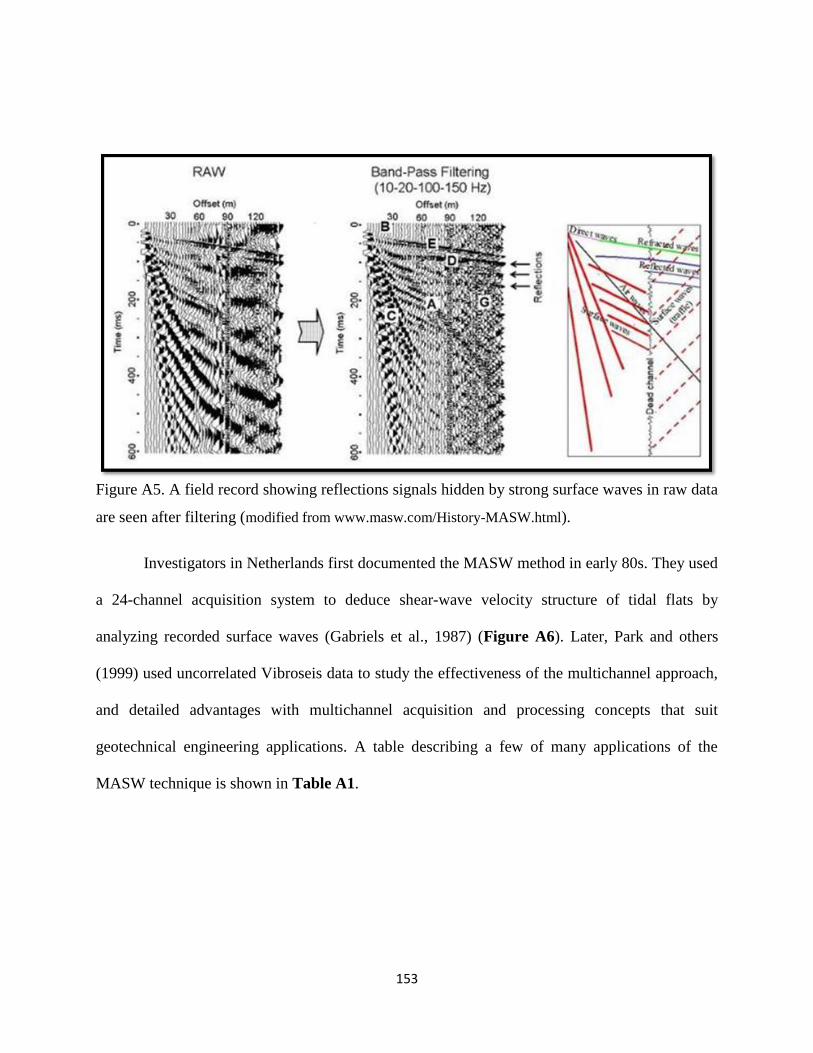
153
Figure A5. A field record showing reflections signals hidden by strong surface waves in raw data
are seen after filtering (modified from www.masw.com/History-MASW.html).
Investigators in Netherlands first documented the MASW method in early 80s. They used
a 24-channel acquisition system to deduce shear-wave velocity structure of tidal flats by
analyzing recorded surface waves (Gabriels et al., 1987) (Figure A6). Later, Park and others
(1999) used uncorrelated Vibroseis data to study the effectiveness of the multichannel approach,
and detailed advantages with multichannel acquisition and processing concepts that suit
geotechnical engineering applications. A table describing a few of many applications of the
MASW technique is shown in Table A1.

154
Figure A6. Summary of work performed by Gabriels et al., (1987) (modified from
www.masw.com/History-MASW.html)
3.3 ADVANTAGES OF MASW
Directly measuring shear-wave velocities from a shear-wave survey is difficult in terms
of maintaining favorable signal-to-noise ratio (S/N) during both data acquisition and data
processing. But MASW method provides fairly favorable and competent results: the data
acquisition is more tolerant in terms of selecting the parameters than any other near-surface
seismic methods and also provides high S/N due to the fact that seismic surface waves are the
strongest seismic waves generated that can travel longer distance than body waves without
suffering from significant noise contamination. Because of high S/N, the MASW method yields
reliable pattern recognition on a seismic record. i.e. it can be used to extract signal in midst of
noise of many natural or cultural activities and also to other types of inherent seismic waves
generated simultaneously.

155
3.4 OVERALL MASW PROCEDURE
The MASW method utilizes multi-channel recording and processing concepts widely
used in near-surface seismology as well as in reflection surveying for oil exploration. The
fundamental mode the Rayleigh is without a doubt one of the most troublesome types of source-
generated noise on reflection surveys. Rayleigh-wave energy is defined as signal in MASW
analysis, and needs to be enhanced during both data acquisition and processing steps. In all kinds
of surface seismic surveys using vertical sources, ground roll takes more than two thirds of total
generated seismic energy and usually appears with the most prominence on the Multi-channel
records. Therefore, generation of ground roll is easiest among all other types of seismic waves.
The field setup is shown schematically in Figure A7. The method first requires measurement of
Table A1. Literature review on applications of MASW technique

156
seismic surface waves generated from various types of seismic sources—such as sledge
hammer—and the propagation velocities of those surface waves is analyzed, and finally the
shear-wave velocity (Vs) variations below the surveyed area that is most responsible for the
analyzed propagation velocity pattern of surface waves is calculated.
The most common procedure that is followed for typical MASW surveys include three major
steps:
4. Data acquisition: acquiring multichannel field records
5. Dispersion analysis: extracting dispersion curves
6. Inversion: Inverting to yield shear-wave velocity variation with depth
Subsequently, a 2-D cross-sectional Vs map may be constructed through an appropriate
interpolation scheme by placing each 1-D Vs profile at surface location corresponding to the
middle of the receiver line. Detailed step by step procedure for each of the step is explained
below and the optimum field parameters are also tabulated.
3.4.1 Field procedure: Data acquisition
This subsection is used to describe the entire field procedure for MASW data acquisition.
Among the active and passive MASW, the active method is the most common type for acquiring
2-D Vs profiles. The maximum depth of investigation (Zmax) that can be achieved from the
survey is usually 10-30 m range and varies with the type of source used. Some of the parameters
related to data acquisition procedure are described below. Table A2 describes the optimum field
parameters for a typical data acquisition procedure, keeping in mind the fact that these can be

157
changed or updated by investigators and practitioners depending upon the requirements and in-
field conditions.
Figure A7. Schematic representation of the active MASW field survey (modified from Park,
2003)
Source
Maximum investigation depth (Zmax) is determined by the longest wavelength (Lmax) of
the surface waves used for the analysis as Zmax=0.5Lmax. Also, Lmax is governed by the energy
and area of impact of the seismic source, which may be controlled type (like the sledge hammer
in case of an active survey) or passive (via a car moving or other kinds of cultural noise).
According to the above relation, the longer Lmax, (deeper the Zmax) can be achieved with a
greater impact power. Some of the commonly used sources include a heavy sledge hammer (10-
20 lb), weight-drop etc. Using an impact plate (also called base plate) will help the source impact
point intrude less into soil. The table below explains different optimum sources for different
investigation depth. For unusually shallow investigation, a relatively light source has to be used

158
so that the dominant frequency can be shifted towards higher frequencies. Ambient noise can be
significantly reduced through multiple impacts and vertical stacking of these impacts therefore is
always recommended, especially if the survey takes place in an urban area.
Seismometers (geophones)
Typically, vertical (instead of horizontal) low-frequency geophones (e.g., 4.5 Hz) are
recommended. Although spike coupled geophones always give the highest sensitivity, the
coupling provided by a land streamer can be equally efficient and is a significant convenience in
field operation. The high end of geophone frequency is not critical as in a typically reflection
survey where any minor drop in sensitivity may become important (see Baker et al., 2000). For
instance, recording and analysis of surface waves up to 450 Hz have been reported by using 4.5-
Hz geophones (Miller et al., 2000) and frequencies up to 1 kHz have been detected from a
hammer blow on an active glacier (Baker et al., 2003).
Field Geometry
Length of the receiver spread (D) should be directly related to the longest wavelength
(Lmax) that can be analyzed, which in turn determines the maximum depth of investigation (Zmax).
Therefore, D usually has to be equal to or greater than Zmax.
D= m Zmax (1<m<3) (3.3)
On the other hand, receiver spacing (dx) is related to the shortest wavelength (Lmin) and
therefore determines the shallowest resolvable depth of investigation (Zmin).
Zmin = k dx (0.3 < k < 1.0)…..(3.4)

159
The source offset distance (x1) is also a major governing factor to predict the degree of
contamination by the near-field effects that indicate a confluence of all adverse influences on
data acquisition, mainly because of the source being too close to the geophones resulting in
“clipping” of the digital record. Although its optimum value is still under debate, a value of 20%
of D is suggested as a minimum and 100% as a maximum. A larger value of x1 and D will
increase the risk of higher-mode domination and reduce S/N for the fundamental mode.
Occationally while performing an active linear survey where the total profile length is
significantly longer than the available geophone spread, sometimes a roll-along spread is used.
In that case, the interval (dSRC) of source-receivers configuration move between 1dx-12dx is
recommended for 24-channel acquisition. This particular variable is also directly related to the
horizontal resolution. Obviously, as the number of available channels increases, the ability to
acquire data along a profile without a roll-along spread is increased.
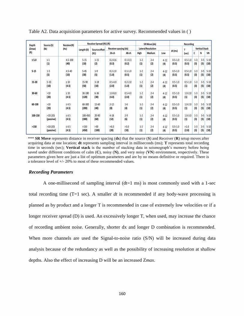
160
Table A2. Data acquisition parameters for active survey. Recommended values in ( )
Recording Parameters
A one-millisecond of sampling interval (dt=1 ms) is most commonly used with a 1-sec
total recording time (T=1 sec). A smaller dt is recommended if any body-wave processing is
planned as by product and a longer T is recommended in case of extremely low velocities or if a
longer receiver spread (D) is used. An excessively longer T, when used, may increase the chance
of recording ambient noise. Generally, shorter dx and longer D combination is recommended.
When more channels are used the Signal-to-noise ratio (S/N) will be increased during data
analysis because of the redundancy as well as the possibility of increasing resolution at shallow
depths. Also the effect of increasing D will be an increased Zmax.
Depth (Zmax) (ft)
Source (S) (lb)
Receiver(R) (Hz)
Receiver Spread (RS) (ft)
Length (D) Source offset (X1)
Receiver spacing (dx)
24-ch 48-ch
SR Move (dx)
Lateral Resolution
High Medium Low
Recording
dt (ms) T(sec)
Vertical Stack
C N VN
≤ 5.0
5-15
15-30
30-60
60-100
100-150
>150
≤ 1(1)
1-5(5)
5-10(10)
>10(20)
>10(20)
>10 (20)(passive)
>10 (20)(passive)
4.5-100(40)
4.5-40(10)
≤ 10(4.5)
≤ 10(4.5)
≤ 4.5(4.5)
≤ 4.5(4.5)
≤ 4.5(4.5)
5-15(10)
5-45(30)
15-90(50)
30-180(120)
60-300(200)
100-450(300)
>150(450)
1-15(2)
1-9(5)
3-18(10)
6-36(30)
12-60(40)
20-90(60)
>30(100)
0.2-0.6(0.3)
0.2-2.0(1.0)
0.5-4.0(2.0)
1.0-8.0(4.0)
2-12(8)
4-18(12)
>6.0(20)
0.1-0.3(0.2)
0.1-1.0(0.5)
0.2-2.0(1.0)
0.5-4.0(2.0)
1-6(4)
2-9(6)
>3.0(10)
1-2(1)
1-2(1)
1-2(1)
1-2(1)
1-2(1)
1-2(1)
1-2(1)
2-4(2)
2-4(2)
2-4(2)
2-4(2)
2-4(2)
2-4(2)
2-4(2)
4-12(4)
4-12(4)
4-12(4)
4-12(4)
4-12(4)
4-12(4)
4-12(4)
0.5-1.0(0.5)
0.5-1.0(0.5)
0.5-1.0(0.5)
0.5-1.0(0.5)
0.5-1.0(0.5)
0.5-1.0(0.5)
0.5-1.0(0.5)
0.5-1.0(0.5)
0.5-1.0(0.5)
0.5-1.0(1)
1.0-2.0(1)
1.0-2.0(1)
1.0-3.0(1)
>1.0(2.0)
1-3(3)
1-3(3)
1-3(3)
1-3(3)
1-3(3)
1-3(3)
1-3(3)
3-5(5)
3-5(5)
3-5(5)
3-5(5)
3-5(5)
3-5(5)
3-5(5)
5-10(10)
5-10(10)
5-10(10)
5-10(10)
5-10(10)
5-10(10)
5-10(10)
*** SR Move represents distance in receiver spacing (dx) that the source (S) and Receiver (R) setup moves after
acquiring data at one location; dt represents sampling interval in milliseconds (ms); T represents total recording
time in seconds (sec); Vertical stack is the number of stacking data in seismograph’s memory before being
saved under different conditions of calm (C), noisy (N), and very noisy (VN) environment, respectively. These
parameters given here are just a list of optimum parameters and are by no means definitive or required. There is
a tolerance level of +/- 20% to most of these recommended values.

161
3.4.2 Field procedure: Data Analysis
The first step in data analysis involves extracting dispersion curves from the data that are
in turn used in the subsequent step of data inversion, whereby a proper layer (shear-wave
velocity-Vs) model is determined such that the theoretical dispersion curves match the measured
ones as close as possible. Usually, the fundamental mode (M0) curve is used. However, recent
studies (Xia et.al., 2000a) suggest that higher-modes can also be utilized to get shear-wave
velocity information.
Concept of Dispersion
In the early stage of surface wave method using monotonic vibrator exciting at a single
frequency (f) at a time, the distance (Lf) between two consecutive amplitude maxima was
measured by scanning the ground surface with a single sensor and an oscilloscope. Then,
corresponding phase velocity (Cf) was calculated as Cf=Lf*f. This measurement was then
repeated for different frequencies to construct a dispersion curve with the assumption that the
fundamental mode (M0) of the surface wave dominate in the field. In early 1900’s this method
was used efficiently by the spectral analysis of surface waves (SASW) method. Instead of trying
to measure the distance of Lf, the method is used to measure the phase difference (dp) for a
frequency (f) between the two receivers a known distance apart from the relationship:
Cf=2*pi*f/dp. This process is repeated for different frequencies to construct a dispersion curve.
The possibility of multi-modal influence during the inversion process is accounted for with the
concept of apparent dispersion curve.
While using a multi-channel approach, however, the user does not calculate individual
phase velocities first, but instead construct an image space whereby dispersion trends are

162
identified from the pattern of energy accumulation (higher amplitude peaks) in this the
frequency-wavenumber domain. Then, necessary dispersion curves are extracted by following
the image trends based on the amplitude anomalies. During this imaging process, a multichannel
record in time-space domain is transformed into either frequency-wave number or frequency-
phase velocity domain. In order to acquire this, the phase-shift method is generally used instead
of any other traditional method like pi-omega or the f-k method because it achieves higher
resolution than the other methods (from www.masw.com).
The Dispersion imaging scheme
The standard data processing scheme is as follows: A multi channel field record (a) is
first decomposed via Fast Fourier Transformation (FFT) into individual frequency components,
and then amplitude normalization is applied to the each component (b). Then, for a given testing
phase velocity in a certain range, necessary amount of phase shifts are calculated to compensate
for the time delay corresponding to a specific offset, applied to individual component, and all of
them are summed together to make a summed energy of (c). This in turn is repeated for different
frequency components. When all the energy is summed in frequency-phase velocity space, it will
show a pattern of energy accumulation that represents the dispersion curve as shown in (d). In
case of multi-modal dispersion, that behavior of energy will appear as multiple energy
accumulations for a given frequency as shown in (e).
3.4.3 Field Procedure: Data Inversion
Inversion in general
Inversion or inversion modelling, in general, attempts to seek the cause to a result when
the result is known. On the other hand, predicting the result from the given cause is referred to as
163
forward modeling. An inversion is known to be unique if there is only one solution to the
problem, and non-unique if multiple solutions exist. It is also called “linear” if the cause-related
relationship is linear as a small change in input yields also a small change in result, whereas
“non-unique” if a small change can give rise to a big change in result.
Typical MASW method inversion
The goal of a field survey and data processing in MASW is to establish the fundamental
mode (M0) dispersion curve as accurately as possible. Theoretical M0 curves are then calculated
for different earth models by using a proper forward modeling scheme (e.g., Schwab and
Knopoff, 1972) to be compared against the measured curve. The process of inversion is based on
the assumption that the measured dispersion curve represents the M0 curve only, not influenced
by any other modes of surface waves. The most important issue with the inversion process is to
determine the best-fit earth model among many different models as efficiently as possible. One
way to check for the closeness between the measured and theoretical curves is the root-mean
square (RMS) error factor. Several other types of inversion are described below.
Multi-modal Inversion
The multi-modal inversion technique utilizes both the fundamental and higher-mode
curves for the inversion. This is done in order to increase the accuracy (resolution) of the final 1-
D Vs profile by narrowing the range of solutions with 1-D Vs profiles otherwise equally well
suited if only the M0 curve is used. This method can also be used to alleviate the inherent
problem with the inversion method of non-uniqueness in general.

164
Dispersion Image Inversion
The method of inversion includes the use of dispersion image data (also called phase-
velocity spectra) instead of dispersion curves, and does not involve the extraction of modal
curves at all (Ryden and Park, 2006; Forbriger, 2003a;2003b). This approach eliminates such
drawbacks with the modal-curve based inversion such as mode-misidentification and mode-mix
problems (misidentifying higher mode curve as a M0 curve) if data acquisition and subsequent
processing are not properly performed. Dispersion curves when misidentified may lead to
erroneous Vs profile because of the lack of compatibility in the inversion process trying to match
measured and theoretical curves.
Raw Data Inversion
As the name suggests, this type of inversion utilizes the raw multichannel record instead
of the one processed for dispersion imaging (Forbriger, 2003b). In the process, the scheme
attempts to compare whole seismic waveforms observed at different distances from the source
with synthetic waveforms generated from a forward modeling scheme. This type of approach
may be advantageous over others for the fact that it is not biased by any other kind of data
processing such as dispersion imaging or curve extraction. At the same time, however, it has to
take into account the attenuation and interference issues, as well as layer parameters, since all of
these can contribute to the shaping of a seismic waveform.
2-D Vs Inversion
This approach uses the final output of 2-D Vs profile from current typical inversion
approach as input to the second phase of the inversion based on a different forward modeling
scheme than previously used. The main objective of this method is to consider the smearing

165
effect caused by the lateral variations during dispersion analysis as much as possible by adopting
another scheme accounting for the local variation of Vs. For this purpose, the Vs structure is
provided by the previous output of the 2-D Vs profile as an initial starting model to account for
the local variations observed within an individual field record to update a certain part of the 2D
Vs model. This initial starting model most likely corresponds to the surface location of the
receiver spread used during data acquisition. Iterations can be performed for a better result. The
main drawback for this method, however, is that it is very computationally intensive.
3.5 TYPES OF MASW METHODS
Depending upon the source used to generate surface waves there are two basic types of
MASW technique: active, where an impact source such as a sledge hammer or a weight drop is
used, and passive method, wherein surface waves are generated by passively recording evergy
from cultural and natural noise such as traffic and tidal motion.
The active (or active-source) survey method is the conventional mode of survey for
collecting MASW. However, there are two sub categories in the passive method, both of which
utilizes surface waves generated passively from ambient cultural noise such as traffic, thunder
etc., and are sometimes used in MASW. The passive-remote method (Park et al., 2004; 2005)
employs a 2-D receiver array such as a cross or circular layout to record passive surface waves.
On the other hand, the passive-roadside MASW method (Park and Miller, 2006) adopts the
conventional linear receiver array and tries mainly to utilize those surface waves generated from
local traffic. For the passive-roadside method, the array is typically deployed along a sidewalk or
on the shoulder of a road , and the survey can continue in a roll-along mode for the purpose of 2-
D Vs profiling.

166
3.5.1 Why do we need passive method?
Although one can achieve reliable Vs estimations with the active-source MASW method,
the depth of investigations is typically only down to a few tens of meters (for example, 30 m).
While this kind of depth is often sufficient for engineering investigations, there are other
instances where the investigation depth is insufficient due to either unusual elastic properties of
the near-surface materials or an usually deep investigation depth sought. Some of the commonly
used active source like a sledge hammer or heavier source like the weight drop can overcome the
limitation; however, the depth range gained may often be trivial as the power delivered by most
of the active sources is not sufficient to achieve a distinguished gain in investigation depth (it is a
strongly nonlinear relationship between depth and power). Even if such a source is invented, it
would likely be uneconomical and impractical.
On the other hand, the surface waves generated from natural or cultural noise are usually
of higher-energy and lower-frequency, with wavelengths ranging from a few kilometers (natural
sources such as wave surf) to a few tens (or hundreds) of meters (cultural sources like traffic)
(e.g., Okada, 2003), providing a wide range of penetration depths and therefore proving to be
more advantageous than the active methods (Park and Miller, 2006). In addition, as the necessity
of performing MASW surveys in urban areas grows, utilizing those pre-existing surface waves
generated by local traffic is found to be a perfect choice recently (Asten, 1978; Louie, 2001;
Okada, 2003; Suzuki and Hayashi, 2003; Yoon and Rix, 2004; Park et al., 2004).

167
Figure A8. Typical field layout for passive remote (left) and passive roadside (right) MASW
surveys
3.5.2 Types of passive MASW methods
As previously mentioned, the passive MASW methods are divided into two subtypes
depending on the field logistics and the type of shear-wave velocity (Vs) profiles (1-D or 2-D)
generated: passive remote (Park et al., 2004) and passive road side (Park and Miller, 2008)
surveys. Examples of field layouts for both passive remote and passive roadside surveys are
shown in Figure A8.
Passive remote survey
The former method utilizes a two-dimensional (2-D) receiver array such as circular, cross
or any other symmetrical shape to record passive surface waves. Although this method involves
laborious field operation and needs more space for deploying the array, results in most accurate
1-D shear-wave velocity profiles (Vs) (Park et al., 2005). For this type of survey any kind of
symmetrical shape like circle, cross, square, triangular or random etc. is used. This study is

168
mainly focused on a study comparing some of the 2-D arrays with that of a random array in
terms of its effect on dispersion analysis and shear-wave velocity extraction. Some of the
commonly used 2-D arrays are shown pictorially in Figure A9.
Passive roadside survey
As mentioned above, this type of MASW method utilizes conventional linear receiver
array and uses local traffic as noise. This method overcomes limitation with the remote in terms
of area of survey and data acquisition procedures, but one has to sacrifice the accuracy of the Vs
evaluation (usually <10%). Because the receivers can be laid linearly and traffic noise can be
used as a source, this set up can be set along a sidewalk, median or on the shoulder of a road and
just as in the active linear array, a roll-along mode can be used for the purpose of 2-D Vs
profiling (from www.masw.com) . Also, while performing this survey, an active impact can be
applied at one end of the array to trigger a long recording. Therefore, from a passive road side
array a combined analysis of surface waves for Vs evaluation can be achieved for both shallow
and deep information simultaneously.

169
Combined active and passive survey
In some cases it is often necessary and useful to combine dispersion images from both
active and passive data: (1) to enlarge the analyzable frequency range of dispersion. (2) to better
identify the modal identity of dispersion trends (active methods results in high frequency range
and passive results in the low frequency range). Although some studies (e.g., Aki, 1965) suggest
that the M0 obtained from passive survey are predominantly Rayleigh waves, recent studies
(Park et al., 2005; 2006) reveal that there is also a strong possibility of higher modes domination.
Figure A9. Examples of 2-D receiver arrays for the passive remote MASW surveys

170
Therefore it is suggested (Park et al., 2005) that a combined analysis would be more reliable for
modal identification.
3.6 SUMMARY
The multi-channel analysis of surface waves (MASW) method is a relatively recently
developed seismic method dealing with relatively lower frequencies and shallow investigation
depth ranges than any other many other conventional seismic methods. The data acquisition and
processing scheme results (Vs information) have proven to be highly reliable in geotechnical
field, even under the presence of higher modes of surface waves and also under various types of
cultural noise. The data processing steps are all automated which makes this method extremely
easy and fast to implement and also very cost-effective. Due to these advantages, this method has
gained significant importance in geotechnical engineering and also in other engineering
communities.

171
APPENDIX B
General computer codes used in modeling studies

172
B1. The general structure for the general.par file is;
101 101 101 1.0
1200 0.00005
2 40 40 40 40 60 20
50.0 50.0 0.0
0.05 60.0 0.05 1.0e+10
2
0.707 0.707 0
1
24
49 96 0
99 54 0
86 14 0
6 35 0
45 84 0
3 73 0
32 75 0
16 3 0
7 11 0
11 54 0
94 52 0
64 40 0
9 22 0
27 55 0
7 27 0
49 74 0
57 71 0
81 36 0
11 79 0
1 30 0
17 82 0
22 5 0
50 72 0
100 62 0
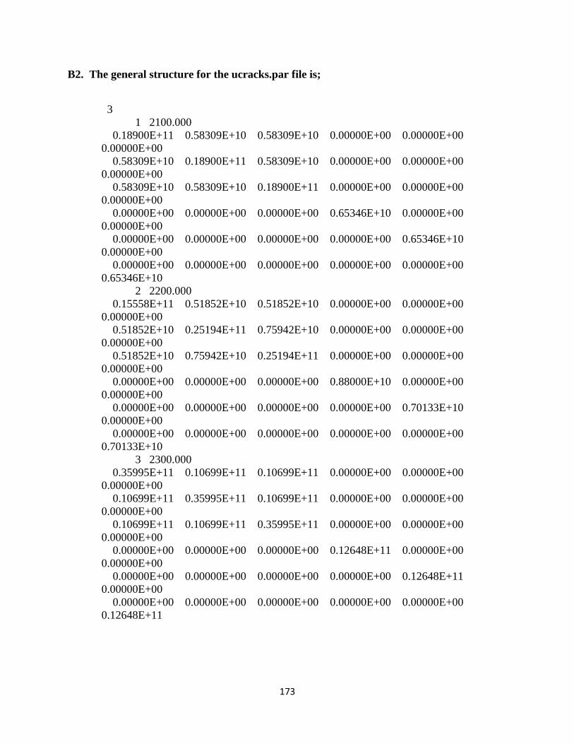
173
B2. The general structure for the ucracks.par file is;
3
1 2100.000
0.18900E+11 0.58309E+10 0.58309E+10 0.00000E+00 0.00000E+00
0.00000E+00
0.58309E+10 0.18900E+11 0.58309E+10 0.00000E+00 0.00000E+00
0.00000E+00
0.58309E+10 0.58309E+10 0.18900E+11 0.00000E+00 0.00000E+00
0.00000E+00
0.00000E+00 0.00000E+00 0.00000E+00 0.65346E+10 0.00000E+00
0.00000E+00
0.00000E+00 0.00000E+00 0.00000E+00 0.00000E+00 0.65346E+10
0.00000E+00
0.00000E+00 0.00000E+00 0.00000E+00 0.00000E+00 0.00000E+00
0.65346E+10
2 2200.000
0.15558E+11 0.51852E+10 0.51852E+10 0.00000E+00 0.00000E+00
0.00000E+00
0.51852E+10 0.25194E+11 0.75942E+10 0.00000E+00 0.00000E+00
0.00000E+00
0.51852E+10 0.75942E+10 0.25194E+11 0.00000E+00 0.00000E+00
0.00000E+00
0.00000E+00 0.00000E+00 0.00000E+00 0.88000E+10 0.00000E+00
0.00000E+00
0.00000E+00 0.00000E+00 0.00000E+00 0.00000E+00 0.70133E+10
0.00000E+00
0.00000E+00 0.00000E+00 0.00000E+00 0.00000E+00 0.00000E+00
0.70133E+10
3 2300.000
0.35995E+11 0.10699E+11 0.10699E+11 0.00000E+00 0.00000E+00
0.00000E+00
0.10699E+11 0.35995E+11 0.10699E+11 0.00000E+00 0.00000E+00
0.00000E+00
0.10699E+11 0.10699E+11 0.35995E+11 0.00000E+00 0.00000E+00
0.00000E+00
0.00000E+00 0.00000E+00 0.00000E+00 0.12648E+11 0.00000E+00
0.00000E+00
0.00000E+00 0.00000E+00 0.00000E+00 0.00000E+00 0.12648E+11
0.00000E+00
0.00000E+00 0.00000E+00 0.00000E+00 0.00000E+00 0.00000E+00
0.12648E+11

174
B3. The general structure for the model.index file is;
1 1 1 1 1 1 1 1 1 1 1 1 1 1 1 1 1 1 1 1 1 1 1 1 1
1 1 1 1 1 2 2 2 2 2 2 2 2 2 2 2 2 2 2 2 2 2 2 2 2
2 2 2 2 2 2 2 2 2 2 3 3 3 3 3 3 3 3 3 3 3 3 3 3 3
3 3 3 3 3 3 3 3 3 3 3 3 3 3 3 3 3 3 3 3 3 3 3 3 3
3 1 1 1 1 1 1 1 1 1 1 1 1 1 1 1 1 1 1 1 1 1 1 1 1
1 1 1 1 1 1 2 2 2 2 2 2 2 2 2 2 2 2 2 2 2 2 2 2 2
2 2 2 2 2 2 2 2 2 2 2 3 3 3 3 3 3 3 3 3 3 3 3 3 3
3 3 3 3 3 3 3 3 3 3 3 3 3 3 3 3 3 3 3 3 3 3 3 3 3
3 3 1 1 1 1 1 1 1 1 1 1 1 1 1 1 1 1 1 1 1 1 1 1 1
1 1 1 1 1 1 1 2 2 2 2 2 2 2 2 2 2 2 2 2 2 2 2 2 2
2 2 2 2 2 2 2 2 2 2 2 2 3 3 3 3 3 3 3 3 3 3 3 3 3
3 3 3 3 3 3 3 3 3 3 3 3 3 3 3 3 3 3 3 3 3 3 3 3 3
3 3 3 1 1 1 1 1 1 1 1 1 1 1 1 1 1 1 1 1 1 1 1 1 1
1 1 1 1 1 1 1 1 2 2 2 2 2 2 2 2 2 2 2 2 2 2 2 2 2
2 2 2 2 2 2 2 2 2 2 2 2 2 3 3 3 3 3 3 3 3 3 3 3 3
3 3 3 3 3 3 3 3 3 3 3 3 3 3 3 3 3 3 3 3 3 3 3 3 3
3 3 3 3 1 1 1 1 1 1 1 1 1 1 1 1 1 1 1 1 1 1 1 1 1
1 1 1 1 1 1 1 1 1 2 2 2 2 2 2 2 2 2 2 2 2 2 2 2 2
2 2 2 2 2 2 2 2 2 2 2 2 2 2 3 3 3 3 3 3 3 3 3 3 3
3 3 3 3 3 3 3 3 3 3 3 3 3 3 3 3 3 3 3 3 3 3 3 3 3
3 3 3 3 3 1 1 1 1 1 1 1 1 1 1 1 1 1 1 1 1 1 1 1 1
1 1 1 1 1 1 1 1 1 1 2 2 2 2 2 2 2 2 2 2 2 2 2 2 2
2 2 2 2 2 2 2 2 2 2 2 2 2 2 2 3 3 3 3 3 3 3 3 3 3
3 3 3 3 3 3 3 3 3 3 3 3 3 3 3 3 3 3 3 3 3 3 3 3 3
3 3 3 3 3 3 1 1 1 1 1 1 1 1 1 1 1 1 1 1 1 1 1 1 1
1 1 1 1 1 1 1 1 1 1 1 2 2 2 2 2 2 2 2 2 2 2 2 2 2
2 2 2 2 2 2 2 2 2 2 2 2 2 2 2 2 3 3 3 3 3 3 3 3 3
3 3 3 3 3 3 3 3 3 3 3 3 3 3 3 3 3 3 3 3 3 3 3 3 3
3 3 3 3 3 3 3 1 1 1 1 1 1 1 1 1 1 1 1 1 1 1 1 1 1

175
APPENDIX C
SAS codes used and the output obtained from mixed model analysis for the inversion data
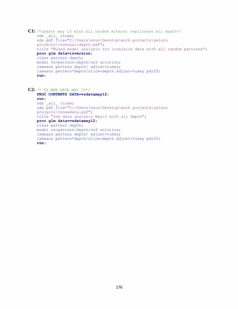
176
C1: /*update may 13 with all random without replicates all depth*/ ods _all_ close; ods pdf file="C:\Users\xsun\Desktop\work projects\yeluru
projects\inveraalldepth.pdf"; title "Mixed model analysis for inversion data with all random patterns"; proc glm data=inversion; class pattern depth; model vs=pattern|depth/ss3 solution; lsmeans pattern depth/ adjust=tukey; lsmeans pattern*depth/slice=depth adjust=tukey pdiff; run;
C2: /* VS NEW DATA MAY 13*/ PROC CONTENTS DATA=vsdatamay12; run; ods _all_ close; ods pdf file="C:\Users\xsun\Desktop\work projects\yeluru
projects\vsnewdata.pdf"; title "new data analysis May13 with all depth"; proc glm data=vsdatamay12; class pattern depth; model vs=pattern|depth/ss3 solution; lsmeans pattern depth/ adjust=tukey; lsmeans pattern*depth/slice=depth adjust=tukey pdiff; run;
177
Vita
Prasanta Malati Yeluru was born in Andhra Pradesh, India, to the parents of Padmanabha
rao and Lalitha Yeluru. She received her Master of Science (Tech) degree in Geophysics in
2001, and worked in National Geophysical Research Institue (NGRI) for about 2 years and went
to York College, Toronto, Canada for further studies. There she received an MS (diploma) in
Geographic Information Systems (GIS). She began her PhD career at University of Tennessee in
August 2006 with Dr. Gregory S Baker. She is happily married to Phaniveer Koti and is a proud
parent of 3 year old daughter, Snigdha Lahari Koti. She will be continuing her career in Dallas,
TX after graduation.