Enhanced Magnetic Reconnection in the Presence of Pressure

Gradients

M.J. Pueschel1, P.W. Terry1, D. Told2,3, and F. Jenko2,3

1 Department of Physics, University of

Wisconsin-Madison, Madison, Wisconsin 53706, USA

2 Max-Planck-Institut fur Plasmaphysik, D-85748 Garching, Germany

3 Department of Physics and Astronomy,

University of California, Los Angeles, California 90095, USA

Abstract

Magnetic reconnection in the presence of background pressure gradients is studied, with special

attention to parallel (compressional) magnetic fluctuations. A process is reported that reconnects

fields through coupling of drift-wave-type instabilities with current sheets. Its time scale is set not

by the reconnecting field but by inhomogeneities of the background density or temperature. The

observed features can be attributed to a pressure-gradient-driven linear instability which interacts

with the reconnecting system but is fundamentally different from microtearing. In particular, this

mode relies on parallel magnetic fluctuations and the associated drift. For turbulent reconnection,

similar or even stronger enhancements are reported. In the solar corona, this yields a critical

pressure gradient scale length of about 200 km below which this new process becomes dominant

over the tearing instability.

1

I. INTRODUCTION

In the space plasma community, magnetic reconnection driven by current gradients – i.e.,

tearing modes – is an area receiving significant attention [1–6]. Meanwhile fusion researchers

have long investigated tearing mode physics (see, e.g., Ref. [7]), and recently important

strides have been made in advancing our knowledge of microtearing (MT) modes [8–10],

which drive reconnection by background electron temperature gradients.

Some studies have focused on the impact of density and temperature gradients on col-

lisionless tearing (CT) modes [11–14], where in the standard picture, such gradients create

stabilizing diamagnetic flows which reduce the growth rate γ relative to its gradient-free value

γ0 (note that the electron temperature gradient may also have an impact, see Ref. [15]). For

strong guide fields and neglecting parallel magnetic fluctuations B‖, this approach (see, e.g.,

Refs. [12, 16]) predicts

γ2 ≈ γ20 −

k2yω

2n

4

(

1 +Ti0

Te0

)2

, (1)

where ky is the instability wave number normalized to the inverse ion sound gyroradius ρs =

cs/Ωi, with the ion sound speed cs = (Te0/mi)1/2 and the ion gyrofrequency Ωi; while Tj0 and

mj are the temperature and mass, respectively, with the ion and electron species indicated

by the indices. The density gradient along the x direction is ωn = Lref/Ln, utilizing the

definitions Lref for the reference (macroscopic) normalization length and Ln = −n0/(∇xn0)

for the density gradient scale length; n0 is the background density, identical for ions and

electrons due to quasineutrality. In the usual local flux tube approximation, both ∇xn0

and n0 are assumed to be constant throughout the simulation domain. Growth rates are

normalized to cs/Lref unless indicated otherwise.

Other work on tearing modes often uses the electron diamagnetic drift frequency ω∗e for

normalization. It is straightforward to convert to that standard: in terms of the normal-

ized density gradient ωn, one has ω∗e = ωnkycs/Lref , where ky is again normalized to ρ−1s .

Thus, this form combines the driving density gradient with the standard normalization of

frequencies for this paper.

A recent study of two-dimensional reconnection in strong guide fields [5] has shown that in

certain parameter regimes, Eq. (1) is no longer valid, but rather found that – under the right

conditions – background gradients may enhance rather than stabilize CT modes. In that

publication, the occurrence of faster modes (relative to CT) in the presence of background

2

gradients is mentioned, along with an attribution of the effect to gradient-driven instabilities.

This paper follows up on those initial findings and describes in detail the process by

which background pressure gradients can enhance reconnecting field growth. It is structured

as follows. After a few words on the gyrokinetic turbulence code Gene, which is used

throughout this paper, it is demonstrated that Eq. (1) accurately predicts the gradient-

modified growth rate in the appropriate limits and in the absence of B‖ fluctuations. While

similar comparisons have been made in the past, demonstrating agreement here serves the

purpose of highlighting the impact of B‖ in the later parts of this paper. A brief excursion is

made in Sec. III, where a new, pressure-gradient-driven instability is presented, which relies

fundamentally on B‖. It is then shown in Sec. IV how reconnection rates may be enhanced by

∇B‖ drifts in high-β cases, counteracting diamagnetic drifts, as well as coupling to pressure-

gradient-driven instabilities. For the solar corona, the latter process is predicted to become

important below a critical gradient length scale, as demonstrated in Sec. V. A summary of

the results of this paper can be found in Sec. VI.

II. CODE-THEORY COMPARISON

As described in detail in Ref. [5] for reconnection physics, the Gene code [17, 18] solves

the gyrokinetic Vlasov-Maxwell system for arbitrary species – here, ions and electrons –

with derivatives along the parallel coordinate treated as ∂/∂z → 0 for the present case.

It is assumed that the reconnecting magnetic field Bx,y ≪ B0, relative to the uniform

background field B0 along z. Note that in the presence of ωn 6= 0, force balance technically

requires ∂B0/∂z 6= 0; this effect, however, is neglected here, a common choice in local flux

tubes. The perpendicular directions x and y are normalized to ρs, whereas z is normalized

to Lref ≫ ρs. The gyrokinetic framework [19] orders out the gyrofrequency time scale,

thus removing fast magnetosonic waves (but retaining parallel magnetic fluctuations B‖).

One may initialize the perturbed part of the distribution function such that it produces

a magnetic field By0 = By(t = 0) at a constant kx = kcs. This drives linear growth of

Bx, derived from the magnetic vector potential A‖, with Bx ≪ By throughout the linear

phase of the instability. Note that all fluctuating magnetic field quantities are normalized

to B0ρs/Lref .

The CT mode grows in the range of wave numbers ky between 0 and kcs – corresponding

3

FIG. 1. Comparison of simulation data with the relative stabilization predicted by Eq. (1) for finite

density gradients ωn ≡ Lref/Ln. In this figure, growth rates are normalized to the inverse Alfven

time γA. Good agreement is seen for these physical input parameters, which lie well in the regime

of validity of the underlying theory. Simulations were run with B‖ deactivated.

to ∆′ values of +∞ and 0, respectively, see Ref. [1] – with the maximum γ occurring roughly

in the center of this ky region. As detailed, e.g., in Refs. [1, 5], one may write the conditions

where analytical theory [16] correctly describes the linear physics of the CT mode as

β

(

1 +Ti0

Te0

)

≫ 2me

mi

isothermal electrons, (2)

β

(

1 +Ti0

Te0

)

≪ 2

(

me

mi

)1/4

no electron FLR, no polarization drift. (3)

Here, FLR stands for finite Larmor radius effects, and β represents the ratio of the electron

kinetic pressure to the magnetic pressure.

To comply with both conditions, the following parameter set is chosen for code-theory

comparisons: Ti0/Te0 = 0.01, hydrogen mass ratio, β = 0.02, and kcs = 0.2. In Fig. 1,

growth rates are shown for the ky = 0.01 tearing mode, as a function of increasing density

gradient ωn. Equation (1) is seen to agree rather well with the simulation data; notably, the

simulated growth rate at ωn = 0 was taken for γ0 to avoid sensitivity to small errors relative

to the analytical small-ky limit. While at small values of β, the impact of B‖ tends to be

very weak, it is to be stressed that these simulations were obtained while artificially setting

B‖ = 0.

4

The growth rates shown in Fig. 1 are normalized to the inverse Alfven time

γA =kcsBy0,max

n0mi

(

2

β

)1/2

, (4)

see Refs. [1, 5]. In standard Gene units, growth rates are normalized to cs/Lref and depend

on the strength of the reconnecting field By0,max. This standard normalization is used in the

next Section, where a slab drift wave is investigated that requires no current gradient for

instability.

III. THE GRADIENT-DRIVEN DRIFT-COUPLING INSTABILITY

In order to illuminate the enhancement of CT growth by pressure gradients for the case

studied in the present paper, it is first necessary to examine a new instability. Consider a

simple, unsheared slab geometry with a density gradient ωn or temperature gradient ωT (of

any species) across the x direction—here, without loss of generality, the case of only a finite

ωn is highlighted. The following assumptions and simplifications are made:

• no parallel variation: ∂/∂z → 0

• no radial variation: kx = 0 ⇒ k⊥ = ky

• no perpendicular magnetic fluctuations: A‖ = 0

• Maxwellian velocity space for the perturbed distributions

More specifically, the driftkinetic limit as applied here refers to a replacement of the Bessel

functions and derived quantities in the gyrokinetic equations with first-order small-argument

expansions. It should be noted that while A‖ is neglected, the coupled Φ-B‖ system is treated

self-consistently through the Poisson equation and Ampere’s law.

In Appendix A, the Vlasov equation and coupled Φ-B‖ field equations for this case

are used to derive a dispersion relation that takes the form of a quadratic equation, see

Eq. (A25). Further assuming low β and small ky lets one compare the relative magnitude of

competing terms, significantly simplifying the dispersion relation and reducing the solution

to Eq. (A31). It is further shown that, consistently using Gene conventions for normaliza-

tion and frequency sign, this equation yields a growth rate and frequency that agrees very

well with the corresponding output from a Maple worksheet evaluating the full dispersion

5

FIG. 2. (Color online) Cartoon picture of the GDC instability. Electrostatic perturbations (green

charges) create drifts (green triangles), which reinforce parallel magnetic perturbations (red circles)

and thus their associated drifts (red triangles). The reinforcing mechanism relies on a gradient of

the background density (blue) or temperature. See the text for more details.

relation, the simulation output from Gene, and the simulation output from the gyrokinetic

code AstroGK [20]. In a last step, parameter dependencies are extracted, yielding for

growth rate and frequency, respectively,

γ ∝ ωnβ1/2 and ω ∝ ωnky . (5)

It is possible to provide a more intuitive picture of the physical mechanisms governing this

instability. In Fig. 2, an electrostatic potential perturbation is shown in green in the form

of alternating positive and negative charges in the y direction. This Φ causes an E×B drift

which advects material from regions of higher and lower background density (or temperature,

in cases where a temperature gradient is present), shown here in blue. The resulting density

perturbation, via pressure balance, leads to a perturbation in B‖ ∝ p⊥ ∝ nT (red circles),

where p⊥ denotes the perturbed perpendicular pressure, at a phase angle of 90 degrees

relative to the original Φ perturbation. Such a B‖, however, necessarily causes a ∇B‖

drift, which, due to its charge-separating property, produces electrostatic perturbations. As

this drift is phase-aligned with the original Φ, reinforcement occurs, and an instability has

arisen (a second solution to the equations corresponds to anti-alignment and results in a

6

damped mode). Based on the above properties, this instability is hereafter referred to as

the gradient-driven drift-coupling (GDC) mode. Both drift reinforcement mechanisms arise

from the Φ-B‖ cross terms in Eqs. (A21) and (A22).

The GDC can be considered a drift-wave-type instability. This is confirmed by the cross

phases between the electrostatic potential Φ and density or temperatures (depending on the

driving gradient), which obey the expected relations, e.g.: Φ×n has a +π/2 phase, Φ×Tj has

−π/2 for ωn drive. This mode fundamentally requires both B‖ fluctuations and background

density or temperature gradients in order to grow; if A‖ is allowed to evolve self-consistently,

one tends to observe A‖ ≪ Φ ∼ B‖. If B‖ (or Φ) is suppressed in a simulation, no GDC

growth is detected.

Different interpretations exist of what constitutes a drift wave. Here, no parallel electron

response exists to connect density and Φ perturbations. Consequently, certain strict defini-

tions of the term “drift wave” may not apply. However, the instability relies fundamentally

on plasma drifts and also exhibits, in general, diamagnetic drifting—for most purposes, the

drift wave label is therefore appropriate.

It is interesting to observe that the calculations in Appendix A also imply that the GDC

is neither simply ion- or electron-type—both CT and MT are electron instabilities. Also

note that modes such as MT generally require finite A‖ to reconnect fields.

Not surprisingly, the GDC grows primarily at kx = 0, as it draws on the free energy

contained in the background gradient(s) along x. Slower growth at finite kx is also observed,

but is found to be negligible when kx ≫ ky. This can be understood by relaxing the kx = 0

assumption in the Appendix and retaining the full k⊥. In the z direction, the mode relies

on the kz = 0 component: if the simulation is restricted to finite values of kz, no growth is

observed. This is simply a consequence of the fact that in the absence of any contribution

at kz = 0, the mode averages out to zero along z.

As illustrated in Fig. 3, the parametric dependencies predicted by the solution of the

dispersion relation are found to hold: as β approaches unity (albeit only indirectly as a

consequence of higher β), very little variation of γ(ky) can be seen for ky ≪ 1. At higher

values, FLR stabilization sets in—note that even in the first-order driftkinetic limit, some

FLR effects are retained, and the mode eventually becomes stable at large ky (larger than

when using the full gyrokinetic approach).

7

FIG. 3. (Color online) GDC growth rate spectra for different values of β: at low pressure, the mode

experiences increasing stabilization in particular at higher ky. All results shown here use ωn = 1

and mi = mH, and are normalized to cs/Ln = cs/Lref . The corresponding normalized diamagnetic

drift frequencies therefore evaluate to ω∗e = ky

.

FIG. 4. (Color online) β dependence of GDC growth (solid black line), with a different regime

appearing at larger values of β & 0.1. This is also reflected by the changing scaling of the mode

frequency ω ∝ k|αω |y (dashed red line). Negative signs of αω correspond to frequencies in the electron

direction. All results shown here use ωn = 1 and mi = mH, and are normalized to cs/Ln = cs/Lref .

Figure 4 shows the influence of β on the peak of the growth rate and on frequency scaling.

Above β ∼ 1, a new regime appears where the frequency changes sign from ion to electron

type (αω indicates the ky scaling exponent of the frequency ω), just as the low-β scaling of

γ ∝ β1/2 breaks down. A similar observation can be made as Ti0 is decreased relative to Te0

8

FIG. 5. (Color online) Scalings of GDC growth rate with different driving gradients: ωn (black

diamonds), ωT i (red triangles), and ωT e (blue squares)—for each curve, all other respective gra-

dients are set to zero. Note that ωn ≡ ωni ≡ ωne due to quasineutrality, leading to a ωn curve

that is approximately twice as steep as the ωTj curves. All results shown here use ky = 0.02 and

mi = mH, as well as Ti0 = Te0.

(not shown), with γ falling in the process.

While the derivation in Appendix A is based on the assumption that only a density

gradient ωn drives the mode, the calculation and results for finite temperature gradients

ωTj are almost identical. This is illustrated in Fig. 5: taking into account that the density

gradient has to be applied to both ions and electrons, leading to doubled growth, the different

gradients have essentially the same impact on γ. The linear dependence is in agreement

with the theoretical predictions. For mixed-gradient drive, one should expect a scaling

γ ∼ 2ωn + ωT i + ωT e. Not shown are the real frequencies—they also scale linearly with the

gradients, with [γ/ω](ωn) ≈ 14, [γ/ω](ωT i) ≈ 2.1, and [γ/ω](ωT e) ≈ −3.3. The sign change

is to be expected for ωT e drive, as it signifies a transition from ion-type to electron-type

mode.

As the reaction of the GDC to finite collisionality may influence its relevance to cer-

tain practical applications, its impact on the growth rate is studied next. Using the same

parameters as below in Sec. IV, along with an electron-ion collisionality ν = 0.1 cs/Lref –

comparable in magnitude to γ for these parameters – one finds only a minimal growth rate

enhancement of ∼ 1%. In effect, the GDC growth rate is thus concluded to be essentially

independent of ν. For more details on the Boltzmann collision operator and definition of

9

the collisionality, see Ref. [5].

Studying more complex scenarios for the GDC has to be deferred to future work. How-

ever, it should be mentioned that the GDC is stabilized by the introduction of a sufficient

amount of background magnetic shear; it is therefore more likely to be prevalent in low-shear

configurations of magnetic confinement fusion experiments. Despite that property, a pos-

sible relation may exist with the compressional electron drift wave mentioned in Ref. [21].

There, an instability is identified which relies on pressure gradients and high β, and which

exists only when taking B‖ fluctuations into account. In general, the GDC as well as its

coupling to tearing modes – as detailed in the next section – could be active in magnetic

confinement experiments. The impact of either, relative to other microinstabilities such as

MT, would depend on the specific physical parameter regime.

In the unsheared slab, the GDC does not exhibit a critical gradient, and it is unstable

– with non-negligible growth rates – even as ky → 0 (but not at exactly ky = 0; there, the

drive term in the Vlasov equation becomes exactly zero, and no mode growth is observed).

While these features make it an interesting candidate for various low-gradient astro- and

space-physical applications, they also mean that nonlinear simulations of GDC turbulence

are problematic. More specifically, since it is impossible to extend the simulation box in

y to the point where the lowest finite ky in the system is linearly stable, and since that

very ky mode necessarily is the most unstable mode, turbulence levels scale with the box

size, and numerical convergence in that direction is impossible. Unless additional degrees of

complexity (such as magnetic curvature or a form of low-ky damping term) are introduced,

simulations can only be considered converged if the full system size is covered in y. That,

however, may be inconvenient due to the periodic boundary conditions. In nonlinear tests

of pure GDC turbulence (i.e., without current sheet drive), the simulations were not well-

behaved. Cases with mixed GDC-CT drive tend to be somewhat more manageable, as shall

be demonstrated later in this paper.

The findings of this Section shall be applied to a reconnecting system in the Section

below, where the direct and indirect impact of B‖ fluctuations on reconnection is studied.

10

IV. ENHANCED RECONNECTION RATES

As described in Ref. [5], finite ωn or ωT in conjunction with self-consistent evolution of

B‖ leads to destabilization of reconnecting field growth, generally with only moderate effects

observed at higher ky and more severe changes at lower ky. Before the focus is turned to

the role of the GDC and similar instabilities in enhancing reconnection rates especially at

these lower ky, the direct effect of B‖ on the tearing mode shall be elucidated, which is

responsible for the more moderate modifications of growth rates seen primarily at higher ky

in the example mentioned above.

A. Counteracting-Drift Destabilization

It is of significance that the standard parameter set in Ref. [5] – which shall also be used

in the present Section – espouses a large β value of 0.3, as it affects the relative magnitudes

of drifts. The other physical parameters are Ti0 = Te0, me = 0.04mi, kcs = 0.2, and

zero collisionality and dissipation. Apart from the temperature ratio, this parameter set is

identical with Case II as described in Ref. [1].

For sufficiently low values of ωn, even relatively low ky tend to exhibit no unexpected

behavior, i.e.: no rapid growth. At ky = 0.02, the following observations can be made. If B‖

is switched off, increasing ωn from 0 to 0.1 leads to a reduction of the linear growth rate by

0.2%—note that the growth rates were extracted with very high precision for this analysis.

This is consistent with diamagnetic drift stabilization, although at these parameters, Eq. (1)

can no longer be expected to yield precise quantitative predictions. Conversely, when B‖

is included, increasing ωn from 0 to 0.1 causes a 1% increase of γ. This opposite behavior

can be explained through the newly activated term in the Vlasov equation: the ∇B‖ drift

requires both B‖ and a non-zero pressure gradient. Especially in cases of high β, it gains

strength relative to the E×B drift and may counteract diamagnetic flow stabilization.

B. Gradient-Enhanced Tearing

The potentially more severe consequence of adding pressure gradients arises from cou-

pling of the CT-driving current sheet to other instabilities, as shall be demonstrated below.

While the present work is focused on coupling specifically with GDC, one could envision, in

11

FIG. 6. (Color online) Tearing growth rates in as a function of wave number ky of the CT mode in

absence of GDC action (black crosses) for ωn = 0 (solid line) and extrapolated to ωn = 0.5 (dotted

line), see the text. The CT in the left plot has stronger tearing drive By0,max = 3.233 than that

in the right (1.617). The other data shown (all with ωn = 0.5) corresponds to GDC growth in Φ

and B‖ (blue diamonds) and the GET effect (red squares), see the text. As a cyan solid line, a fit

curve is shown to illustrate the k2y dependence of GET. The effect of changing CT drive relative

to ωn drive on GET is apparent when comparing both plots. The normalized diamagnetic drift

frequencies are 0.5ky for either case, whereas the inverse Alfven times γA evaluate to 1.67 (left)

and 0.84 (right).

principle, other drift-wave-type instabilities taking its place.

A clarifying comment shall be made before presenting any results, however. The terms

tearing and reconnection are used for a variety of physical effects and scenarios, with different

meanings found in different publications. In the present work, both refer – interchangeably –

to growth in the reconnecting field Bx and the resulting rearrangement of magnetic topology

around X and O points. Thus, tearing includes but is clearly not limited to the tearing mode

(CT in the present nomenclature), and tearing allows no inferences about the free energy

source of reconnection.

Figure 6 shows the CT growth rate in black, both for ωn = 0 and ωn = 0.5, with the

latter extrapolated to illustrate the subdominant regime at low ky. For the extrapolation,

simulations with lower ωn are used, and the moderate enhancement of γ (as opposed to the

rapid growth discussed below) seen in these simulations – which varies little over the entire

ky range – is used to obtain γ at ωn = 0.5. The resulting values match the high-ky direct

12

FIG. 7. (Color online) Radial mode structures Re(A‖), in arbitrary units, for CT (solid lines: red

for ky = 0.2, blue for ky = 0.16), for the driving current sheet (black dotted line), and for GET

(pink dashed line, ky = 0.22). Here, a particularly small By0,max was chosen to obtain GET growth

at negative ∆′.

results at this gradient setting very precisely. Also included, in red, is the enhanced growth

rate of the process which henceforth will be referred to as gradient-enhanced tearing (GET).

Growth rates for CT and GET are extracted by measuring the reconnecting field Bx as a

function of time—since the GDC does not excite Bx,y fluctuations, this does not measure

linear GDC growth (which instead is apparent in Φ and B‖).

In Fig. 6, the blue curve labeled GDC marks growth of the linear system in the absence

of a current gradient. In terms of numerical resolutions, the GDC requirements are similar

to those for CT (see Ref. [5]), apart from the radial direction which technically requires

only one mode at kx = 0—compare, however, the corresponding comment in the previous

Section.

The effect of ∇B‖ on CT growth rates, as discussed earlier, can be seen by comparing the

solid black curve (CT at ωn = 0) and the dotted black curve (CT at ωn = 0.5). A moderate

enhancement is found to exist throughout the range of unstable ky.

The picture becomes more complex when looking at the GET simulation results at ωn =

0.5, as shown by the dashed red curves: while following the dotted black curve at high ky,

growth rates much larger than that of the CT are observed at low ky. As ky → 0, the

growth rate of the GDC is attained (in units of cs/Lref). The deviation from the original

CT behavior becomes even more striking when lowering the driving By0,max, as seen in the

right plot. Here, the growth rates especially at low ky take on more and more the nature

13

FIG. 8. (Color online) Contours of the magnetic potential A‖ for two narrowly spaced moments

in time: earlier contours are black dashed lines, later ones red solid lines. Only a subsection of the

simulation box is shown, focusing on the X point, where reconnection is clearly visible. The data

stems from a GET simulation at negative ∆′ with a large ωn relative to the tearing mode drive.

of the GDC rather than the CT mode. One consequence is that CT growth occurs even

for ky ≥ kcs if the GDC is sufficiently strong (not shown in the figure), despite the fact

that this corresponds to the region of ∆′ ≤ 0. The relevant mode structures are shown in

Fig. 7, including GET for one such case (ky = 0.22). Note that due to the dominant kx = 0,

the GDC structure (not shown) is constant in x. Due to its coupling to the current sheet,

GET results in a corresponding mode structure when CT is subdominant. As soon as the

red GET curve becomes identical with the black CT curve in Fig. 6, its structure matches

exactly that of the CT.

In light of the mode parities in Fig. 7, it is to be stressed that GET, while not a tearing

mode in the strict sense of the word, is indeed able to reconnect magnetic fields at an

elevated rate. This is illustrated in Fig. 8, where reconnection at the rate of the GDC occurs

at ky = 0.22 > kcs (i.e., ∆′ < 0), as a consequence of a large ωn.

Destabilization of reconnection by GDC action at lower ky can be understood from a

heuristic calculation. CT simulations – here, in Ref. [5], and equivalently in Ref. [1] – are

technically nonlinear but yield linear growth rates and describe linear physics. This stems

14

from the fact that the current sheet implementation occurs purely in the perturbed modified

distribution function g(k) through the Vlasov nonlinearity∑

k′(k′xky − kxk

′y)χ(k

′)g(k − k′),

with χ containing the current sheet (rather than a perturbation thereof).

Here, the effect on the linear growth rate is of interest. It is a mode-coupling term in the

gyrokinetic response for g(k, ω) that is proportional to g(k − k′, ω − ω′), nominally making

it phase-incoherent with g(k, ω). One may use the renormalization procedure of resonance

broadening theories [22] to calculate iterative mode-coupling contributions in order to find

the piece that is phase-coherent with g(k, ω). To model the effect on the growth rate, the

frequency of the gyrokinetic operator is taken here to represent the frequency of the linear

dispersion relation – which is not be modeled explicitly in the following – and find the

nonlinear decrement from the renormalized nonlinearity.

The nonlinear gyrokinetic response of the GET effect at wavenumber k and frequency ω

can be written as

−iωg(k, ω) =∑

k′,ω′

(k′xky − kxk

′y)χ(k

′, ω′)g(k − k′, ω − ω′) . (6)

GET is observed for the first component in the nonlinearly interacting triplet of (k, ω),

(k′, ω′), and (k − k′, ω − ω′) with a complex frequency ω to be determined from the renor-

malized dispersion relation to be derived here. The second triplet component is the current

sheet that drives the CT, which resides in A‖, and therefore in χ at k′x = kcs and k′

y = 0.

It is stationary (whereby the nonlinearity physically reduces to a linear term, albeit one

with mode coupling), converting the frequency summation to the operation ω′ → 0. Lastly,

the GDC is the third component in the triplet, with kx − k′x = 0 (which makes kx = kcs)

and ky − k′y = ky > 0. The current sheet and GDC act as the dominant terms in the

k′ summation of the Vlasov nonlinearity, with the generalized potential χ(k′) reducing to

−v‖A‖(kcs, 0) (ignoring gyroaverages), with v‖ denoting the parallel velocity coordinate.

Determining the coherent renormalization of the right-hand side of Eq. (6) is done by

iterating on the mode coupling to find a nonlinear component that is phase-coherent with

g(k). The (technically nonlinear) evolution of g(k − k′, ω − ω′) = g(k − k′, ω) is expressed

in terms of its linear GDC drive and its mode coupling as follows,

−i (ω − ωGDC) g(k− k′, ω) =∑

k′′′

(

k′′′x (ky − k′

y)− (kx − k′x)k

′′′y

)

χ(k′′′)g(k− k′ − k′′′, ω) , (7)

where the appearance of the complex GDC frequency leads to a linear response ω = ωGDC

15

for χ = 0, consistent with GDC wavenumber k − k′. The wavenumber k′′′ = −k′ selects the

coherent renormalized response. Solving this expression for g(k − k′, ω) and substituting it

into Eq. (6) yields

−iωg(k, ω) = −∑

k′(k′xky − kxk

′y)

2|χ(k′)|2−i(ω − ωGDC)

g(k, ω) , (8)

where the right-hand side is a standard propagator renormalization or resonance broadening

decrement (see, e.g., Ref. [23]). The solution of the resulting dispersion relation is

ω =1

2

ωGDC ±(

ω2GDC + 4

∑

k′

(k′xky − kxk

′y)

2|χ(k′)|2)1/2

≡ ωGET , (9)

whose dominant branch reduces to ωGET = ωGDC for a negligible current sheet in χ.

Assuming a weak but non-zero current sheet, the first and (at least at low ky) dominant

root of the dispersion relation becomes

ωGET = ωGDC

(

1 +1

ω2GDC

∑

k′

(k′xky − kxk

′y)

2|χ(k′)|2)

, (10)

which, for ωGDC = iγGDC, results in overall growth that experiences a stabilizing force at

finite ky that is proportional to k2yB

2y0,max, which is precisely what was shown to be the case

in Fig. 6.

More specifically, quadratic fits to the data at low ky are shown for both plots. One

may compare these fits quantitatively with the predicted values from Eq. (10), using for

this simple argument the thermal velocity (i.e., v‖ ∼ 1 in normalized units) in the definition

of χ, as well as kcsA‖ ∼ By0,max. For the first case, By0,max = 3.233, one thus obtains

a stabilization ∆γ about 25% weaker than the fit curve. Repeating this procedure for

the second case, By0,max = 1.617, very similarly yields a ∆γ about 25% lower than the

corresponding fit curve. Therefore, despite the heuristic nature of the calculation, it is able

to capture the dependencies on ky and By0,max correctly, as well as provide a fairly good

quantitative estimate for the stabilization.

Having established the physical process behind GET, the focus is now shifted to the

regulation of either growth rate through the driving gradients. CT growth scales with

γA ∝ By0,max, whereas in units of cs/Lref , the value of γGDC depends only on ωn (if ωTj = 0)

and yields results independent of By0,max (when outside the GET regime). Note that Lref

enters both into the normalization of the reconnecting field via By0,max → By0,maxB0ρs/Lref

16

and the GDC growth rate measured in units of cs/Lref . Consequently, Lref can be seen

as a measure of the scale separation between reconnecting and background field, while

simultaneously determining the value of ωn for a given Ln.

Consider a hydrogen plasma in a uniform magnetic field B0 which is subjected to a

(perpendicular) density gradient ωn = 1, equivalent to normalizing macroscopic scales to

the gradient scale length. For simplicity, assume β = 2 and n0 = Ti0 = Te0 = 1. Now

a current is introduced in the parallel direction which produces a sinusoidal field By at

kx = 1 which is constant in y. This scenario is susceptible to a CT mode with a growth rate

maximum of γCT ∼ 0.03γA; at the same time, it provides the ingredients for GDC/GET,

this time with a growth rate on the order of γGET ∼ cs/Ln (= kyω∗e, even though the results

are insensitive to the precise value of ky → 0). Translating this value into Alfvenic units

yields γGET ∼ γA/By0,max, making the relative CT-GET impact

γCT

γGET

∼ 0.03By0,max (11)

where the usual normalization for By0,max evaluates to units of B0ρs/Ln. By choosing a value

for the free parameter By0,max, one can pick the dominant instability; in the process possibly

creating a GET growth rate γGET ≈ γGDC ≫ γCT, along with γGET ≫ γA. Alternatively,

one may view By0,max as fixed and vary ωn, with the same relative results. By dint of these

relations, GET may therefore take the role of ultrafast reconnection—as opposed to the CT

mode which is sometimes referred to as fast reconnection.

C. Impact On Turbulence

Nonlinear particle acceleration through parallel electric fields may provide large energies

even when By0,max and B0 are significantly separated. This situation is investigated in

Ref. [24], where the focus lies on reconnection turbulence driven by a term in the Vlasov

equation∂g

∂t= . . .− ωdr

(

gky=0(t)− gky=0(t = 0))

, (12)

where ωdr is a driving frequency; dissipation is provided by a collision operator. Note that

this form of the nonlinear drive constitutes an improved version of that presented in Ref. [5].

Before applying GET to a fully nonlinear scenario, it should be noted that the turbulent

parallel electric field E‖ – as well as the heating rate j‖E‖ (with the parallel current j‖) –

17

scales to a significant degree in accordance with expectations based on the linear growth

rates. While Ref. [24] focuses on a case without background gradients, for the present work

simulations were performed at ωn ranging from 0.1 to 1. Even when linear growth rate

enhancements were small (i.e., γ & γ(ωn = 0)), parallel electric fields and heating rates were

significantly increased. As was discussed in Sec. III, box size settings – which, in numerically

converged regions, have no impact on volumetric heating rates in the absence of ωn – severely

affect j‖E‖ even at ωn = 0.1.

A brief comment on the heating rate and the parallel electric field: consistent with

gyrokinetic literature, the moniker parallel is used for a number of quantities that are parallel

to the background magnetic field – v‖, A‖, B‖, j‖ – and could equivalently be labeled with

the subscript z. Magnetic field perturbations will lead to a slight misalignment of field lines

relative to the background field, but it can be shown through ordering relations that the

aforementioned quantities are hardly affected; e.g., v‖ = vz + δ, where δ → 0 in gyrokinetic

ordering. This, however, is not the case for E‖, where this misalignment has to be taken

into account, see Ref. [24].

For the latter case, with the default box sizes from Ref. [24] of 62.8ρs × 62.8ρs, contours

of the turbulence are shown in Fig. 9. The tendency of turbulent structures to cover the

whole simulation box is apparent not only in Φ (where the GDC exerts direct influence) but

also in A‖, where GET imprints CT with GDC features. In particular, B‖ (not shown in

the figure) and Φ – whose field equation is coupled to that of B‖ – see marked increases in

amplitude relative to the case with ωn = 0, with strong heat and particle transport along

x. Interpreting the results of such a simulation in the context of physical heating therefore

becomes a difficult undertaking. The addition of GDC-stabilizing properties to the physical

setup, such as background magnetic shear or curvature, may alleviate these issues; due to

the associated complexity, such studies will have to be deferred to future work.

While more research into the physical and numerical properties of this mixed reconnection

and drift-wave turbulence will be necessary to understand all relevant mechanisms, these first

results indicate that GDC and GET do not merely affect linear growth rates but can also be

expected to enhance heating in turbulent scenarios. Given the difficulties and open questions

that stem from nonlinear simulations, however, in the following the focus is returned to linear

enhancement of reconnection rates and their possible role in coronal settings.

18

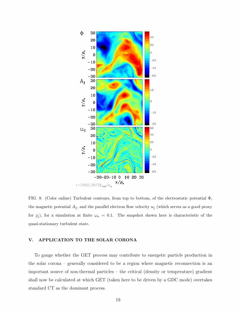
FIG. 9. (Color online) Turbulent contours, from top to bottom, of the electrostatic potential Φ,

the magnetic potential A‖, and the parallel electron flow velocity u‖ (which serves as a good proxy

for j‖), for a simulation at finite ωn = 0.1. The snapshot shown here is characteristic of the

quasi-stationary turbulent state.

V. APPLICATION TO THE SOLAR CORONA

To gauge whether the GET process may contribute to energetic particle production in

the solar corona – generally considered to be a region where magnetic reconnection is an

important source of non-thermal particles – the critical (density or temperature) gradient

shall now be calculated at which GET (taken here to be driven by a GDC mode) overtakes

standard CT as the dominant process.

19

As per Refs. [25, 26], typical parameters for the solar corona are n ∼ 109 cm−3 for the

density, B0 ∼ 100G for the magnetic field, and L ∼ 109 cm for the parallel extent of the

domain and choice of Lref ; with a temperature T = 106 K which shall be applied here to both

ions and electrons. From these quantities, one arrives at β = 0.00035, cs = 9.1×106 cm/s,

and ρs = 9.5 cm. These values are identical with the default settings used in the Corona

section of Ref. [24].

Furthermore, using the respective domain size and magnetic field from Ref. [25], one

has a driving kx = 0.0004 and field By0,max = 7.5× 106 in the usual normalized units

(corresponding to By0 = 2−1/2By0,max = 5G). Simulating at lower By0,max and using the

standard γA scaling, one can extract the CT growth rate; the corresponding simulations

were performed with Nx = 16384 grid points in x. In addition, one can directly obtain

γGDC(ωn) ≈ γGET(ωn) (with similar results expected for ωTj which are set to zero here) for

these parameters.

In units of cs/Lref , the growth rates thus read: γCT ∼ 1.3 and γGET = 0.026ωn; or,

equivalently, γCT/γA ∼ 5.7×10−6 and γGET/ω∗e = 65 (assuming ky = kcs in the definition of

the diamagnetic drift frequency). Based on these values, the critical gradient length scale

where γCT = γGET becomes

Lcritp = 0.02Lref = 2×107 cm , (13)

where Lp = Ln or Lp = LT . Clearly, this value scales with By0,max: smaller values will result

in an earlier onset of GET—an alternative interpretation is that for a given ωn,T , there

exists a minimal By0,max below which GET will dominate. If gradients occur on smaller

scale lengths than Lcritp , and presuming that three-dimensional CT is not drastically faster

than its two-dimensional counterpart, one can expect GET to play a role in reconnecting

fields. It should be stressed that Lp ≫ Lcritp may be necessary for GET to be straightforward

to distinguish from CT observationally.

While large-scale density or temperature fluctuations in the corona are on the order

of Lp ∼ 108 cm, filamentation can create significantly smaller-scale fluctuations [27] with

potentially higher ωn,T . In particular, the above Lcritp should constitute a realistic scenario for

corona physics, making GET activity an interesting candidate for processes behind coronal

heating. Moreover, the filament-like structures in the turbulence described in Ref. [24] are

creating small-scale, self-consistent gradients in n and T , while mergers of circular structures

20

are found to create heating bursts consistent with nanoflares [28]. Therefore, one may assume

that nanoflare intensities can be affected by the GET effect.

VI. SUMMARY

Gradients in the background density and their impact on tearing mode growth rates have

been studied, in conjunction with the investigation of a new drift-wave instability referred

to as gradient-driven drift-coupling (GDC) mode.

The standard picture of reconnection stabilized by diamagnetic flows in response to such

gradients is confirmed quantitatively in the applicable limits. However, when considering

higher β values and including B‖ effects, the ∇B‖ drift is found to counteract the E×B drift,

under the right circumstances leading to net destabilization of the CT mode. For all cases

studied here, however, destabilization has been moderate, with at most a few 10% increase

in growth rates.

With both B‖ and density or temperature gradients ωn,T , a drift-wave-type mode becomes

unstable which couples the ∇B‖ and E×B drifts. More specifically, a fluctuation in the

electrostatic potential Φ reinforces, via its associated E×B drift and the background gradient

ωn,T , the fluctuation in B‖. The latter, in turn, reinforces Φ via the∇B‖ drift. Therefore, the

name gradient-driven drift-coupling instability is introduced for this mode. In unsheared

slab geometry, it has no critical gradient and is independent of the mode number ky at

sufficiently low ky.

When both CT and GDC activity are present in a system, the latter may couple to the

current sheet driving the former, leading to reconnection being observed on time scales asso-

ciated with GDC growth. As the GDC is regulated by ωn,T – as opposed to the reconnecting

field strength By0,max, which governs CT growth – there now exists a means of inducing re-

connecting field growth, in principle, at a rate much faster than the inverse Alfven time;

or, alternatively, at a velocity much faster than the Alfven speed. For this process, dubbed

gradient-enhanced tearing, or GET, to be dominant over standard CT growth in the solar

corona, a sufficiently large ωn,T is required. Using typical parameters, the corresponding

critical gradient scale length is shown to be Lcritp = 2×107 cm, below which the GDC and

thus GET grow more quickly than CT—a value that is consistent with expectations for the

solar corona.

21

In terms of turbulence, the impact of GET is significant: heating rates are found to be

strongly enhanced even at moderate ωn. However, the increases in j‖E‖ – and turbulent

amplitudes in general – are not and cannot be made to be converged in the perpendicular

box sizes, as turbulent structures are gravitating towards the lowest wave numbers in the

system. As even lower wave numbers are included by increasing box sizes, the turbulence

therefore changes quantitatively, leading to stronger heating among other consequences. To

obtain properly converged answers regarding the impact of pressure gradients on reconnec-

tion turbulence, one must therefore either take the full system size into account – with some

consequences for the boundary conditions – or introduce more realistic modeling of stabi-

lizing effects such as background magnetic shear. Such efforts shall be the subject of future

investigation.

ACKNOWLEDGMENTS

The authors would like to express their gratitude to E.G. Zweibel, V.V. Mirnov, M. Swis-

dak, J.F. Drake, and M. Velli for discussions and helpful insights. In part, the numerical

studies in this work were performed on the Kraken XT5 HPC system through XSEDE grant

PHY130013. The research leading to these results has received funding from the European

Research Council under the European Union’s Seventh Framework Programme (FP7/2007-

2013)/ERC Grant Agreement No. 277870.

Appendix A: Derivation

Following Ref. [5] and the simplifications delineated in Sec. II, the normalized gyrokinetic

Vlasov equation (note that ∂t → iω instead of −iω is used to match Gene’s frequency sign

convention) reads

iωgj = −ωnF0ikyχ = −ωnF0iky

(

J0(λj)Φ +Tj0µ

qj

2J1(λj)

λj

B‖

)

, (A1)

with λj ≡ k⊥(2Tj0mjµ/(B0q2j ))

1/2 and χ = J0(λj)Φ + [(Tj0µ)/qj][(2J1(λj))/λj]B‖ in the

absence of A‖-type fluctuations. Defining ≡ −ωnky/ω, one thus obtains

gj = F0

(

J0(λj)Φ +Tj0µ

qj

2J1(λj)

λj

B‖

)

. (A2)

22

Additionally, the background distribution can be written as F0 ≡ π−3/2e−v2‖−µB0 . Next, the

field equations (setting the Debye length λD = 0) can be written as

Φ =C3M00 − C2M01

C1C3 − C22

(A3)

B‖ =C1M01 − C2M00

C1C3 − C22

(A4)

M00 =∑

j

qjnj0πB0

∫

J0gjdv‖dµ (A5)

M01 =∑

j

qjnj0πB3/20

vTj

k⊥

∫

µ1/2J1gjdv‖dµ (A6)

C1 = k2⊥λ

2D +

∑

j

q2jnj0

Tj0

(1− Γ0) (A7)

C2 = −∑

j

qjnj0

B0

(Γ0 − Γ1) (A8)

C3 = − 2

β−∑

j

2nj0Tj0

B20

(Γ0 − Γ1) (A9)

where Γk ≡ Ik(bj)e−bj and bj ≡ k2

⊥Tj0mj/(q2jB

20). One may define

D ≡(

C1C3 − C22

)−1. (A10)

Next, gj will be inserted into M0x, which in turn goes into the fields.

First, these are the relevant integrals, with η√µ ≡ λj:

∞∫

−∞

e−v2‖dv‖ = π1/2 (A11)

∞∫

0

J0(η√µ)2e−µB0dµ =

1

B0

e−η2/(2B0)I0

(

η2

2B0

)

≡ Γ0

B0

(A12)

∞∫

0

J0(η√µ)J1(η

√µ)µ1/2e−µB0dµ =

η

2B20

(Γ0 − Γ1) (A13)

∞∫

0

J1(η√µ)2µe−µB0dµ =

η2

2B30

(Γ0 − Γ1) (A14)

Thus,

M00 =∑

j

qjnj0

(

Γ0Φ +2Tj0

qj

1

2B0

(Γ0 − Γ1)B‖

)

(A15)

M01 =∑

j

qjnj0B1/20

vTj

k⊥

(

η

2B0

(Γ0 − Γ1)Φ +2Tj0

qj

η

2B20

(Γ0 − Γ1)B‖

)

(A16)

23

These reduce to

M00 = Φ∑

j

qjnj0Γ0 + B‖∑

j

nj0Tj0

B0

(Γ0 − Γ1) (A17)

M01 = Φ∑

j

nj0Tj0

B0

(Γ0 − Γ1) + B‖∑

j

2nj0T2j0

qjB20

(Γ0 − Γ1) (A18)

or, implicitly defining the quantities A,

M00 = ΦA1 + B‖A2 (A19)

M01 = ΦA2 + B‖A3 (A20)

Note that for singly charged ions, A1,A3 → 0 in the zeroth-order driftkinetic limit due to

quasineutrality.

With these definitions, the field equations become

Φ = DC3(

ΦA1 + B‖A2

)

−DC2(

ΦA2 + B‖A3

)

(A21)

B‖ = DC1(

ΦA2 + B‖A3

)

−DC2(

ΦA1 + B‖A2

)

(A22)

Therefore,

B‖ =Φ(C1A2 − C2A1)

(D)−1 − C1A3 + C2A2

, (A23)

allowing for the elimination of Φ, which in turn yields (with all real C and A)

(D)−1 = C3A1 +C3A2 (C1A2 − C2A1)

(D)−1 − C1A3 + C2A2

− C2A2 −C2A3 (C1A2 − C2A1)

(D)−1 − C1A3 + C2A2

, (A24)

or, alternatively,

(D)2 (−C3C1A1A3 + C3C2A1A2 + C3C1A22 − C3C2A2A1

+ C2C1A2A3 − C22A2

2 − C2C1A3A2 + C22A3A1)

+D (C1A3 − 2C2A2 + C3A1)− 1 = 0 . (A25)

The condition for instability (i.e., for Im() 6= 0) therefore becomes

− 4 (−C3C1A1A3 + C3C2A1A2 + C3C1A22 − C3C2A2A1

+ C2C1A2A3 − C22A2

2 − C2C1A3A2 + C22A3A1)

> (C1A3 − 2C2A2 + C3A1)2 . (A26)

24

From evaluation at typical parameters (here, ωn = B0 = Te0/Ti0 = 1 and ky = β = 0.01,

hydrogen mass ratio), one can compare the constituting quantities:

C1 ≈ 1.0×10−4 C2 ≈ 1.5×10−4 C3 ≈ −204.0 D ≈ −49.0 (A27)

meaning −2/β ≈ C3 ≫ C1 ∼ C2. Similarly,

A1 ≈ −1.0×10−4 A2 ≈ 2.0 A3 ≈ −3.0×10−4 (A28)

Thus, the magnitude of the relevant terms can be estimated:

C3C1A1A3 ∼ 10−9 C3C2A1A2 ∼ 10−5 C3C1A22 ∼ 10−1

C3C2A2A1 ∼ 10−5 C2C1A2A3 ∼ 10−11 C22A2

2 ∼ 10−7

C2C1A3A2 ∼ 10−11 C22A3A1 ∼ 10−15

C1A3 ∼ 10−8 C2A2 ∼ 10−4 C3A1 ∼ 10−2 (A29)

Clearly, the third term dominates the condition for instability in magnitude. As it has

negative sign, the condition is fulfilled. Examining the second-to-last term in Eq. (A26)

in relation to the third, one can also see that Im() ≫ Re(). With this ordering, the

equation for reduces to

(D)2C3C1A22 +DC3A1 − 1 = 0 . (A30)

The solution is therefore

=−C3A1 ± 2(C3C1A2

2)1/2

2DC3C1A22

= −2.55×10−3 ± 0.0714i (A31)

for the parameter choice mentioned above, which translates to

γ, ω = 0.1399, 0.004996 . (A32)

By comparison, solving the full gyrokinetic dispersion relation in Maple yields a very similar

γ, ω = 0.1399, 0.004848 , (A33)

which, in turn, is nearly identical with the gyrokinetic simulation results from Gene simu-

lations,

γ, ω = 0.1398, 0.004844 , (A34)

25

and runs performed with AstroGK,

γ, ω = 0.1397, 0.004851 . (A35)

Note that the latter are shown here in Gene normalization.

To obtain parametric dependencies as applicable near the above point in parameters

space, one may write the complex frequency components as

γ ≈ ωnkyIm()

ω = −ωnkyRe()

Im()2(A36)

and thus

γ = ωnky|D|(−C3C1A22)

1/2 (A37)

ω = −1

2ωnkyDC3A1 (A38)

based on Eq. (A31). Writing out the constituting terms gives the following expressions:

γ = ωnky

(

2

β+∑

j

2nj0Tj0

B20

(Γ0 − Γ1)

)1/2(∑

j

nj0Tj0

B0

(Γ0 − Γ1)

)

×(

∑

j

q2jnj0

Tj0

(1− Γ0)

)1/2/

(

∑

j

q2jnj0

Tj0

(1− Γ0)

)

×(

2

β+∑

j

2nj0Tj0

B20

(Γ0 − Γ1)

)

+

(

∑

j

qjnj0

B0

(Γ0 − Γ1)

)2

(A39)

ω = −ωnky2

(

− 2

β−∑

j

2nj0Tj0

B20

(Γ0 − Γ1)

)

×(

∑

j

qjnj0Γ0

)/

(

∑

j

q2jnj0

Tj0

(1− Γ0)

)

×(

− 2

β−∑

j

2nj0Tj0

B20

(Γ0 − Γ1)

)

−(

∑

j

qjnj0

B0

(Γ0 − Γ1)

)2

(A40)

which, by comparing the different C and using C3 = −2/β (in the low-β limit), can be

simplified to

γ = ωnky

(

2

β

)−1/2(

∑

j

nj0Tj0

B0

(Γ0 − Γ1)

)(

∑

j

q2jnj0

Tj0

(1− Γ0)

)−1/2

(A41)

ω = −ωnky2

(

∑

j

qjnj0Γ0

)(

∑

j

q2jnj0

Tj0

(1− Γ0)

)−1

(A42)

26

In the low-ky, driftkinetic limit, one can write (with bj = k2yTj0mj/(q

2jB

20))

Γ0 ≈ 1− bj 1− Γ0 ≈ bj Γ0 − Γ1 ≈ 1− 3

2bj ≈ 1 (A43)

where the linear contribution has to be retained in the first expression because of the zero-

order term canceling due to quasineutrality, see below; whereas in the last expression the

linear contribution – which is quadratic in ky – is dominated by the zero-order term. There-

fore

γ = ωnky

(

2

β

)−1/2(

∑

j

nj0Tj0

B0

)(

∑

j

k2y

nj0mj

B20

)−1/2

(A44)

ω = −ωnky2

(

∑

j

qjnj0

(

1− k2y

Tj0mj

q2jB20

)

)(

∑

j

k2y

nj0mj

B20

)−1

(A45)

Since∑

j qjnj0 = 0 due to quasineutrality, one can write

γ = ωn

(

2

β

)−1/2(

∑

j

nj0Tj0

)(

∑

j

nj0mj

)−1/2

(A46)

ω =ωnky2

(

∑

j

nj0Tj0mj

qj

)(

∑

j

nj0mj

)−1

(A47)

These expressions are valid to first order in ky. With a hydrogen plasma (qi = −qe and

me ≪ mi) and assuming Ti0/Te0 ≫ me/mi, this becomes

γ = ωn

(

βni0

2mi

)1/2

(Te0 + Ti0)insert−−−→m,n,T

ωn

√

2β = 0.14 (A48)

ω =ωnky2

Ti0

qi

insert−−−→m,n,T

ωnky2

= 0.005 (A49)

in good agreement with the aforementioned results.

In summary,

γ ∝ ωnk0yβ

1/2 ω ∝ ωnkyβ0 (A50)

Note that both analytical and simulation approaches using zeroth-order (in ky) approxima-

tions for J0 and J1 yield different results for the frequencies.

[1] B.N. Rogers, S. Kobayashi, P. Ricci, W. Dorland, J. Drake, and T. Tatsuno, Phys. Plasmas

14, 092110 (2007)

27

[2] J.F. Drake, M. Swisdak, T.D. Phan, P.A. Cassak, M.A. Shay, S.T. Lepri, R.P. Lin,

E. Quataert, and T.H. Zurbuchen, J. Geophys. Res. 114, 05111 (2009)

[3] W. Daughton, V. Roytershteyn, B.J. Albright, H. Karimabadi, L. Yin, and K.J. Bowers,

Phys. Rev. Lett. 103, 065004 (2009)

[4] E.G. Zweibel, E. Lawrence, J. Yoo, H. Ji, M. Yamada, and L.M. Malyshkin, Phys. Plasmas

18, 111211 (2011)

[5] M.J. Pueschel, F. Jenko, D. Told, and J. Buchner, Phys. Plasmas 18, 112102 (2011)

[6] R. Numata, W. Dorland, G.G. Howes, N.F. Loureiro, B.N. Rogers, and T. Tatsuno, Phys. Plas-

mas 18, 112106 (2011)

[7] J.W. Connor, S.C. Cowley, R.J. Hastie, T.C. Hender, A. Hood, and T.J. Martin, Phys. Fluids

31, 577 (1988)

[8] H. Doerk, F. Jenko, M.J. Pueschel, and D.R. Hatch, Phys. Rev. Lett. 106, 155003 (2011)

[9] W. Guttenfelder, J. Candy, S.M. Kaye, W.M. Nevins, E. Wang, R.E. Bell, G.W. Hammett,

B.P. LeBlanc, D.R. Mikkelsen, and H. Yuh, Phys. Rev. Lett. 106, 155004 (2011)

[10] H. Doerk, F. Jenko, T. Gorler, D. Told, M.J. Pueschel, and D.R. Hatch, Phys. Plasmas 19,

055907 (2012)

[11] M. Swisdak, B.N. Rogers, J.F. Drake, and M.A. Shay, J. Geophys. Res. 103, 1218 (2003)

[12] E. Tassi, F.L. Waelbroeck, and D. Grasso, J. Phys. Conf. Series 260, 012020 (2010)

[13] D. Grasso, F.L. Waelbroeck, and E. Tassi, J. Phys. Conf. Series 401, 012008 (2012)

[14] O. Zacharias, R. Kleiber, and R. Hatzky, J. Phys. Conf. Series 401, 012026 (2012)

[15] J.W. Connor, R.J. Hastie, and A. Zocco, Plasma Phys. Control. Fusion 54, 035003 (2012)

[16] F. Porcelli, Phys. Rev. Lett. 66, 425 (1991)

[17] F. Jenko, W. Dorland, M. Kotschenreuther, and B.N. Rogers, Phys. Plasmas 7, 1904 (2000)

[18] see http://genecode.org for code details and access

[19] A.J. Brizard and T.S. Hahm, Rev. Mod. Phys. 79, 421 (2007)

[20] R. Numata, G.G. Howes, T. Tatsuno, M. Barnes, and W. Dorland, J. Comp. Phys. 229, 9347

(2010)

[21] E.A. Belli and J. Candy, Phys. Plasmas 17, 112314 (2010)

[22] T. H. Dupree, Phys. Fluids 9, 1773 (1966)

[23] W. Horton and D. Choi, Phys. Reports 49, 273 (1979)

[24] M.J. Pueschel, D. Told, P.W. Terry, F. Jenko, E.G. Zweibel, V. Zhdankin, and H. Lesch,

28

Astrophys. J. Suppl. Ser. 213, 30 (2014)

[25] P.A. Cassak, J.F. Drake, and M.A. Shay, Astrophys. J. 644, L145 (2006)

[26] E.R. Priest and T.G. Forbes, Astron. Astrophys. Rev. 10, 313 (2002)

[27] A.F. Rappazzo and M. Velli, Phys. Rev. E 83, 065401 (2011)

[28] E.N. Parker, Astrophys. J. 330, 474 (1988)

29