energy system decarbonization and productivity gains

Article

Energy system decarboniz
ation and productivitygains reduced the coupling of CO2 emissions andeconomic growth in 73 countries between 1970and 2016
Graphical abstract

Highlights

d We estimate impacts of five mechanisms on nations’ CO2

emissions over 1970–2016

d Without these mechanisms, emissions grow as fast as the

economy

d Energy system decarbonization was the primary mechanism

for high-income countries

d Productivity gains were the primary mechanism for low-

income countries

Wang et al., 2021, One Earth 4, 1–11November 19, 2021 ª 2021 The Author(s). Published by Elsevierhttps://doi.org/10.1016/j.oneear.2021.10.010

Authors

Ranran Wang, Valentina A. Assenova,

Edgar G. Hertwich

[email protected]

In brief

To successfully combat climate change

we must understand what mechanisms

are most effective in reducing CO2

emissions while maintaining economic

growth. Existing literature proposes

divergent estimates on this relationship.

Here, we study emission trends for 73

countries between 1970 and 2016 and

identify five mechanisms that reduced

CO2 emissions. We show that energy

system decarbonization and economic

productivity gains were themost effective

mitigation mechanisms during times of

growth. However, emission-reduction

trends in all observed countries fall short

of meeting net-zero targets by 2050.

Inc.ll

OPEN ACCESS
ll
Article

Energy system decarbonization and productivity gainsreduced the coupling of CO2 emissions and economicgrowth in 73 countries between 1970 and 2016Ranran Wang,1,2,3 Valentina A. Assenova,4 and Edgar G. Hertwich3,5,6,*1Institute of Environmental Sciences (CML), Faculty of Science, Leiden University, 2333 Leiden, the Netherlands2University of Twente, Faculty of Engineering Technology, Drienerlolaan 5, 7522 Enschede, the Netherlands3Yale School of the Environment, 195 Prospect Street, New Haven, CT 06511, USA4Management Department, The Wharton School, University of Pennsylvania, Philadelphia, PA 19104, USA5Department of Energy and Process Engineering, Norwegian University of Science and Technology, Kolbjørn Hejes v 1B, Trondheim 7491,

Norway6Lead contact

*Correspondence: [email protected]://doi.org/10.1016/j.oneear.2021.10.010

SCIENCEFORSOCIETY Fearing negative repercussions for economic growth, climate policy is not on trackto meet the Paris Agreement temperature target. However, the academic literature disagrees on both theimpact of economic growth on climate mitigation and the effectiveness of various mitigation mechanismson CO2 emissions reduction. Here, we investigate the relationship between CO2 emissions and economicgrowth in 73 countries during the period 1970–2016. We find that in the absence of mitigation mechanisms,emissions would have indeed grown at the same rate as the economy. However, these five mechanisms—energy system decarbonization, electrification, increased economic productivity, deindustrialization, andwinter warming—are identified as successfully reducing emissions by 19 gigatonnes, mostly during periodsof economic growth. Yet, observations indicate that emissions reduction rates consistent with the ParisAgreement could be achieved while maintaining economic growth only if energy systems are more rapidlydecarbonized.

SUMMARY

Nations must curtail carbon dioxide (CO2) emissions by 7% per annum to meet the Paris Agreement temper-ature targets. A perceived economic growth-climate mitigation trade-off has diminished political will to act.However, there is no scholarly consensus regarding the magnitude of the trade-off between economicgrowth and CO2 mitigation and a lack of ex post evidence regarding the extent to which mitigation measurescan effectively lower CO2 emissions. Here, we present a structural equation model integrating emissions andeconomic and energy system characteristics over the period 1970–2016 to empirically assess mechanismsthat influence the GDP-CO2 relationship for 73 countries. Robust to various model specifications and statis-tical tests, we found a simple unitary scale effect between per capita GDP and per capita CO2 emissions,while five emission-reduction mechanisms, principally energy system decarbonization and productivitygains, collectively contributed to global emission reductions by 19 petagrams. Within the observed year-to-year emissions development, reductions at a rate consistent with the Paris Agreement can be achievedin about 10% of instances while maintaining economic growth.

INTRODUCTION

The world achieved explosive growth of the human population

and unprecedented levels of economic welfare in the past two

centuries through increased and improved utilization of fossil

fuels.1 In the 2015 Paris Agreement, 192 countries agreed to

One Earth 4, 1–11, NovThis is an open access article und

halt the global temperature rise at well below 2�, preferably

1.5�.2 Achieving a 1.5�C warming goal requires cutting global

greenhouse gas (GHG) emissions by more than 7% per year

on average from 2020 on.3 However, the latest UN synthesis of

the nationally determined contributions (NDCs) under the Paris

Agreement warns that current climate commitments, even if fully

ember 19, 2021 ª 2021 The Author(s). Published by Elsevier Inc. 1er the CC BY license (http://creativecommons.org/licenses/by/4.0/).

A B Figure 1. Emissions-economy pathways:

CO2-GDP relationships and time series ob-

servations

(A) A schematic illustration of the characteristic

CO2-GDP relationship; (B) CO2-GDP relationships

suggested by the CO2-GDP elasticity estimated by

previous studies (ranging from �0.3 to 2.5), which

are reviewed in detail in Note S1 and Table S1,

supplemental information; (C–E) observed (165

countries, 1970–2020) CO2 emissions per capita

related to fossil fuel combustion and industrial pro-

cesses versus real GDP per capita in constant US

dollars (C), the energy intensity of GDP (D), and CO2

intensity of primary energy supply (E); (C) shows a

relatively strong positive correlation between GDP

and CO2 emissions. A reduced-form analysis that

controls for the country- and year-fixed effects in-

dicates a CO2-GDP elasticity = 0.53 (p < 0.001), i.e.,

a 1% of GDP growth is associated with a 0.53%

increase in CO2 emissions on average. The less than

unitary CO2-GDP relationship referred to as relative

decoupling is consistent with the findings of many

recent empirical studies, e.g., Burke and co-

workers.22–25,27,31,32 Despite a lack of empirical proof, the reduced emission rate is commonly attributed to the falling energy intensities of GDP illustrated in (D),

given that energy supplies have been decarbonizing at slow rates across the world (E).

llOPEN ACCESS Article

Please cite this article in press as: Wang et al., Energy system decarbonization and productivity gains reduced the coupling of CO2 emissions andeconomic growth in 73 countries between 1970 and 2016, One Earth (2021), https://doi.org/10.1016/j.oneear.2021.10.010

realized, are far from adequate to meet the target of the Paris

Agreement.4 Worse, countries have not been on track to

achieving their past NDC pledges, and global GHG emissions

continued to grow in 2019 and fell by only 6.4% in 2020 owing

to the COVID-19 pandemic.3,5 A first step in ratcheting up the

NDCs will occur at the upcoming 26th conference of the parties

(COP26) of the UNFCCC in Glasgow in November 2021.

The political commitments and negotiations about emission

reductions are invariably tied up with the question of economic

growth, both through the fundamental question of how to recon-

cile emission reductions with the economic development

required to attain most other sustainable development goals

and through the tricky issues of how to share the cost of emission

reductions as well as the remaining emissions budget.6,7 Studies

of the empirical relationship of CO2 emissions and economic

development8 have focused on estimating the CO2-GDP elastic-

ity, i.e., the percentage change of a country’s CO2 emissions per

capita for every 1% increase in the GDP per capita (Figures 1A

and 1B). They have variously shown everything from a 0.3%

decrease to a 2.5% increase in CO2 emissions for every percent

growth in a country’s GDP9–27 (for details, see Note S1 and Table

S1 in supplemental information). As a result of these disparate

findings, policymakers have not been able to rely on empirical

analysis in weighing the trade-offs of potentially conflicting social

goals. Variation in these estimates has been attributed to sam-

ple-selection issues (see Figure 1B) and the potential for

spurious results given insufficient consideration of statistically

problematic properties of the investigated data (i.e., non-statio-

narity,28 endogeneity,26,29 and cross-sectional heterogene-

ity14,30). We hypothesize, meanwhile, that the failure of the

empirical studies to identify a simple monocausal relationship

between GDP and CO2 emissions lies in the separate influence

of independent causal mechanisms on historical CO2 emission

pathways.

The recent success of selected countries to reduce their CO2

emissions even during periods of economic growth has been

2 One Earth 4, 1–11, November 19, 2021

noted prominently in the literature.33–35 However, we do not

have an adequate understanding of the mechanisms that have

enabled such a hopeful development. Existing knowledge about

how to reduce anthropogenic CO2 emissions while not impeding

economic development was predominantly derived using ex

ante analyses.36–38 Ex ante analyses predict emissions based

on the modeling of presumed causal relationships of, e.g., elec-

trification, solar power deployment, and other energy system

transformations, on CO2 emissions. Empirical studies have

shown, ex post, that historical developments can differ qualita-

tively and quantitatively from ex ante engineering estimates, con-

firming or disproving the hypothesized relationships adopted by

ex ante studies.39,40 Moreover, emission reductions in highly

developed countries have been posited by the environmental

Kuznets curve (EKC) hypothesis.13,41–43 It suggests that people

have an increased willingness to pay for environmental quality

once they become sufficiently affluent. Recent studies, however,

have disputed the methodological robustness of the EKC litera-

ture and essentially undermined the validity of the EKC hypothe-

sis as an explanation for emission reduction during periods of

economic growth.14,44 Another explanation for declining emis-

sions accompanying economic growth is the offshoring of heavy

industries with increased trade, but the evidence about these

mechanisms remains contradictory.25–27,29,45

Here, we propose a structural equation model of the relation-

ship between GDP and CO2 emissions, which can investigate

the role of additional factorsmediating theGDP-CO2 relationship

and apply it to an extensive dataset covering 73 economies over

the period 1970–2016 (detailed in Note S2 and Table S2, supple-

mental information). The results show that, keeping other factors

constant, per capita CO2 emissions change in lockstep with per

capita GDP. We test various mechanisms suggested in the liter-

ature to reduce CO2 emissions and our model identifies the

following emission-reduction mechanisms as influential: (1) in-

creases in economic productivity, (2) energy system decarbon-

ization (including both increasing renewable shares and the

Table 1. The empirical relationships between CO2 emissions per capita and economic, energy system, and temperature-related

factors based on the benchmark model

Factors affecting per capita CO2 emissionsa Explanatory variables Coefficients Bootstrap SE 95% Bca CI

Economic development

Economic growth Db GDP/p 1.0194***c 0.1082 0.8150 1.2406

(1)d Increases in productivity D A∙L/p �0.4824*** 0.0923 �0.6764 �0.3184

(2) Deindustrialization - D Vsh_Ind �0.7724*** 0.2890 �0.3107 �1.4585

Energy system transition

(3) Decarbonization

Fossil fuel to renewables D TPESsh_renw �1.4942*** 0.1333 �1.7125 �1.1761

Coal to natural gas - D TPES_FFsh_coal �0.5883*** 0.1063 �0.3568 �0.7541

(4) Electrification D Electrification �1.2589*** 0.6091 �2.4193 �0.4669

Other

(5) Winter warming D Tmin �0.0050*** 0.0007 �0.0065 �0.0037

n (countries/regions) 73

N (observations) 3,283

R2 0.45

*p < 0.05, **p < 0.01, ***p < 0.001 (two-sided Z test, 1,000 bootstrap runs).aFull results are provided in Table S3, Note S3, including the non-statistically significant emission effects (p R 0.05), estimates of the GDP equation,

and SEs and CIs estimated without bootstrapping.bD is the first difference operator.cThe CO2 elasticity of GDP is not statistically different from 1 (prob > c2 = 0.81).dChanges of the factors in desirable directions, as indicated by the negative coefficients, correspond to the emission-reduction mechanisms (1)–(5) we

referred to throughout the manuscript.

llOPEN ACCESSArticle


fuel switching from coal to gas), (3) electrification, (4) winter

warming, and (5) deindustrialization (see explanation of the se-

lection and test of these five and other suggested mechanisms

in the experimental procedures). Over the past 47 years, energy

system decarbonization contributed the most (i.e., 28%) to

emission reductions at high economic development levels

when electrification was saturated, while at low development

levels, increases in economic productivity contributed the most

(i.e., 36%) to emission reductions in addition to being a driver

of economic growth. Therefore, our study resurrects the debate

about the role that economic growth plays in anthropogenic CO2

emissions and identifies vital energy systems and economic

development characteristics that contribute to emission reduc-

tions. Our findings also inform the policy debate around these is-

sues by showing that, without unprecedented transformations,

no country is likely to achieve economic growth annually while

gradually cutting CO2 emissions, i.e., by the 2% (Tanzania) to

17% (Qatar) annual average reduction rate required to reach

net-zero by 2050. The ex post empirical evidence we present

can be valuable for informing emission-reduction policies, given

that there can be only a few years left at our current rate of emis-

sions before we exceed the 1.5�C carbon budget.46

RESULTS

Emission-reduction mechanisms during economicgrowthUsing our benchmark model, we find that a 1% increase in GDP

per capita was associated with a 1% increase in CO2 per capita

on average, holding all other factors constant (Table 1; full results

of the benchmark model are available in Note S3 and Table S3,

supplemental information). Our estimates of this elasticity are

robust to various model specifications. The specifications ac-

count for the emission effect of economic growth in previous

years, the asymmetric emission effects of economic expansions

versus recessions, emission effects related to countries’ devel-

opment levels, and using a three-equation (CO2, primary energy

use, and GDP) simultaneous model. In addition, our estimates

are robust to models estimated with 5-year rolling windows to

eliminate the influence of cyclical variations and using alternative

data sources. Results of the various tests are available in Note S4

and Tables S4–S6, supplemental information.

In addition to changes in GDP per capita, five factors

describing changes in the economy, energy system, and tem-

perature were identified to significantly affect observed carbon

emission reductions in our sample (Table 1). We find that while

economic productivity drives economic growth, at the same

time a 1% increase in a country’s overall economic productivity

was associated with roughly a 0.5% annual reduction in its CO2

emissions per capita (Table 1). Combining the growth-inducing

and direct effects of productivity on CO2 emissions, a 1% rise

in productivity causes a net increase in emissions of 0.5%.

Such mediating effect was not found for other growth-driving

factors (Table S3), indicating that the type of economic growth

plays a role in a nation’s emission pathway. Consistent with

the conventional wisdom that deindustrialization—for example,

through amove to services—reduces CO2 emissions, our results

also show that CO2 emissions per capita were reduced by about

0.8% as the share of non-industrial output in GDP grew by 1%.

Our results further reveal that the majority (>80%) of the emis-

sion-reduction effect of deindustrialization was attributable to a

reduction in primary energy use (Table S5).

One Earth 4, 1–11, November 19, 2021 3



Energy system decarbonization and electrification also

contributed to reduced carbon emissions. A 1% annual increase

in the share of renewable energy used in energy supply (referred

to as ‘‘renewables share’’ thereafter) was associated with a 1.5%

yearly decrease in CO2 emissions per capita on average (Table

1). The three-equation (CO2, primary energy use, and GDP)

simultaneous model further reveals that two-thirds of the renew-

able shares’ emission-reduction effect was attributable to

lowering carbon intensity, and the rest to improving energy effi-

ciency (Table S5). Specifically, a 1% annual increase in renew-

ables share is associated with a 1% yearly decrease in CO2

emissions per capita (see ‘‘CO2 equation’’) and a 0.5% decrease

in primary energy use per capita (see ‘‘energy equation’’); the

relationship between primary energy use and CO2 emissions

per capita is unitary (CO2 equation). Our result could indicate

that renewable energy was more efficient than fossil fuels in

serving energy demand during the observation period. However,

this result could also be attributable to different accounting

approaches used for calculating the primary energy content of

fossil and non-fossil fuels.47

Among fossil fuels, we find that decarbonization owing to nat-

ural gas displacing coal (i.e., fuel switching) also contributed to

significant CO2 emission reductions. We estimate that annual

CO2 emissions per capita decreased by 0.6% for every 1% in-

crease in the share of natural gas substituted for coal (Table 1).

As further revealed by results from the three-equation simulta-

neous model (Table S5), much of the decarbonization effect of

fuel switching was attributable to reducing carbon intensity,

and the rest was attributable to improving energy efficiency.

Specifically, for every 1% increase in the share of natural gas

substituted for coal, the direct reduction of CO2 emissions per

capita was 0.4% (CO2 equation), and the impact via primary en-

ergy use was 0.2% (energy equation). With the same fuel mix,

electrification contributed to reduced carbon emissions by

improving energy efficiency. Every 1% increase in the share of

electricity in the final energy supply was associated with a

1.3% decrease in annual per capita CO2 emissions.

Winter warming also reduced national CO2 emissions per cap-

ita (Table 1). Our results showed that an increase in the average

temperature of the coldest month by 1�C was associated with a

0.5% annual reduction in carbon emissions during the observa-

tion period. Finally, only 0.02%–0.04% of the annual emission

reduction (p < 0.05) was attributable to the time-invariant charac-

teristics of a few developed and emerging European economies

(Bulgaria, France, Ireland, Poland, Romania, Sweden, and the

UK) and Mozambique. The time-invariant characteristics can

be, for instance, countries’ political institutions48 geography, cul-

ture, and renewable energy potentials.49

All factors included in Table 1 had significant effects on chang-

ing annual CO2 emissions per capita over the 47 years of data in

our sample. The effects of the five emission-reduction mecha-

nisms were estimated precisely (p < 0.001) despite variation

across time and countries’ development levels. For deindustrial-

ization and electrification, the magnitudes of their emission-

reduction effects depended on further characteristics of the

two processes, as illustrated by the relatively greater confidence

intervals (CIs) shown in Figure 2A. The goodness-of-fit of our

model, as measured by R2, was 0.45, as compared with R2 sta-

tistics of between 0.05 and 0.27 from prior models examining the


empirical relationship between changes in GDP and CO2 emis-

sions per capita.20,22,50,51 Statistical tests show that our results

are robust to alternative model specifications and data sources

(Note S4 and Tables S4–S6 in supplemental information) and

are verified by statistical tests for multicollinearity, non-stationar-

ity, and cross-sectional correlation (Note S5 and Tables S7–S11,

supplemental information).

Emissions cuts contributed by the reductionmechanismsTo quantify the total CO2 emissions contributions of the main

mechanisms over 1970–2016, we combined the estimates from

the benchmark model with data from the observed year-by-

year changes in economic output in our data (3,283 country-

year observations, Equation 7 in experimental procedures). The

results from these analyses showed that changes in GDP per

capita lead to an increase in CO2 emissions per capita adding

up to a total of 16–29petagrams (Pg) (95%CI) of global CO2emis-

sions during 1970–2016 (Figure 2B). Please note that changes in

per capita GDP comprised both periods of growth (76% of in-

stances) and periods of decline. A decline of GDP per capita

commonly contributed to a decline in per capita CO2 emissions.

This finding is consistent with prior findings that increases inGDP

per capita are a primary driver of increases in CO2 emissions per

capita.53–55 Our results are based on empirically estimated rela-

tionships. By contrast, prior assessments have relied mostly on

index-decomposition analysis and have assumed that changes

in each mechanism contribute to proportional and independent

changes in carbon emissions; for instance, a doubling of energy

intensity leads to a doubling of emissions. Contrary to these as-

sumptions, our empirically estimated relationships reveal that

most of themainmechanisms have had non-proportional effects

on carbon emissions (Table 1) arising from stochastic influences

and interdependencies.

Aside from the emission effects associated with changes of

GDP per capita, the five emission-reduction mechanisms

contributed to global CO2 emission reduction over 1970–2016.

Specifically, increases in economic productivity, energy system

decarbonization, electrification, deindustrialization, and winter

warming resulted in emission reductions of about 6, 5, 4, 2,

and 2 Pg, respectively (Figure 2C). The emission reductions

were contributed by the desirable changes of the economic, en-

ergy, and temperature factors, which were present in 42%–69%

of the country-year sample, depending on the factors of interest.

In the rest of the samples, changes of these factors contributed

to increasing emissions, e.g., by shifting from gas to coal or

increasing the share of industry in theGDP. Considering all coun-

try-year samples, only economic productivity and electrification

changes contributed to net CO2 emission reductions globally, as

shown in Figure 2B. The mix of upward and downward trends of

other factors resulted in minimal or upward effects (only in the

case of the share of renewables) on CO2 emissions globally

over the past 47 years.

Understanding what mechanisms contributed to past CO2

emission reductions for countries of varying levels of economic

development is informative for both the design and the evalua-

tion of emission-abatement policies (Figure 2D). We find that

emission reductions in developed economies were always and

increasingly dominated by energy system transition, especially

Figure 2. Effects of the economic, energy, and temperature factors on CO2 emissions derived from the benchmark model

The same labeling as in Table 1: economic growth rate (1), economic productivity (2), deindustrialization (3), decarbonization by shifting to renewables (4) or from

coal to natural gas (5), electrification (6), and winter warming (7). They are consistently color coded in the subplots. Error bars show the ranges calculated from the

95% bias-corrected and accelerated (BCa) confidence intervals (Table 1).

(A) Estimated CO2 elasticities (coefficients in Table 1, black bars) and distributions of the 1,000 bootstrapped estimates (shaded areas). The color saturation

indicates the probability that the CO2 elasticity is at a given value plotted in a ‘‘visually weighted’’ fashion based on Burke et al.52

(B and C) Total contributions to emissions changes (TEC) (all 3,283 observations) and emissions reductions (TEC_R) (based on observations where the

mechanisms resulted in emissions reduction effects; sample coverage in the parenthesis), respectively (in petagrams [Pg]). Error bars show the ranges calculated

from the 95% BCa confidence intervals (Table 1). See Figure S1 for a breakdown by decade and developed/developing countries.

(D and E) (D) TEC_R by decade and development level. Sample coverage by development level and decade are provided in the parentheses. The green bars

represent emission-reduction effects of energy decarbonization, i.e., (4) and (5). (E) The emission implication of economic development: economic growth rate (1)

and productivity (2).



decarbonization. At high levels of economic development, de-

carbonization became evermore critical for CO2 emission reduc-

tions. The importance of energy transitions (i.e., decarbonization

and electrification) for CO2 reductions has grown steadily since

the 1980s (from 36% to 57%) in developed countries. By

contrast, across developing countries increased economic pro-

ductivity and electrification were the primary mechanisms, ac-

counting for 60% of their CO2 emission reductions. Moreover,

our results show that CO2 emission reductions in developing

economies have grown since the 1990s and dominated global

mitigation over the last decade (comprising 64% of global emis-

sion reductions in the 2010s). However, more rapid CO2 emis-

sion increases due to rapid economic growth over the same

period outpaced these reductions.

On a global level, increasing economic productivity was a uni-

versal mechanism of both reducing per capita CO2 emissions

and driving up economic growth in our sample (Figure 2E). This

explains much of the emission reductions achieved in devel-

oping economies during the 2000s (47% of total reductions)

and over the past 47 years (36% of total reductions). The emis-

sion-reducing effect of productivity growth declined in impor-

tance in developed countries, while it rose from zero to quite

crucial for developing economies. The small relative importance

of productivity growth as a CO2-reduction mechanism in devel-

oped countries as a whole is due mainly to the steady and

notable emission-reduction effects contributed by energy sys-

tem decarbonization in developed countries since the 1970s

(see Note S6 and Figure S1, supplemental information). As

such, our results show that the emission-increasing effects of

economic growth can be reduced when countries increase eco-

nomic productivity. Thus, increases in economic productivity—

and not merely in output—may be needed to help developing

economies balance the dual objectives of economic growth

and environmental sustainability.


A B

C

D

Figure 3. GDP per capita growth rates

compatible with stabilizing or declining CO2

per capita emission rates under future ‘‘busi-

ness-as-usual’’ development

(A–D)The percentile distribution of the maximum

annual GDP growth rates compatible with a zero-

emissions growth rate in the same year (A). The

maximum compatible GDP growth rates are equiv-

alent to the sum of the emission reduction outcomes

of the same-year changes in economic productivity,

deindustrialization, energy system decarbonization,

and electrification over 1970–2016. The shading

represents the range based on the 95% confidence

interval for the estimated effects. The remaining

panels show the corresponding distribution of

global population, GDP, and CO2 emissions of fossil

fuel combustions and industrial processes (B),

country-year observations for developed (OECD)

and developing (non-OECD) countries, respectively

(C), and country-year observations over different

decades since the 1970s (D). Emission reductions associated with economic recessions (periods of negative per capita GDP growth) are not the focus of this

analysis and thus are not shown here.



Our model accurately predicts net emission reductions for

83% of the observed occurrences of declines in carbon emis-

sions during periods of economic growth over 1970–2016.

Such consistency is most notable for 15 developed and devel-

oping economies where our estimated reductions match 95%

of observed, repeated occurrences (R15 years) of emission

decline coupled with GDP growth (see Figure S2, supplemental

information). Energy system decarbonization dominated the

recent CO2 emission reductions achieved during periods of eco-

nomic growth in the UK, Denmark, New Zealand, Uruguay, and

the US. In France, Ireland, Sweden, and Poland, the most recent

CO2 emission reductions during periods of economic growth

were driven primarily by time-invariant country characteristics.

These characteristics and their emission-reduction effects

need to be explored further in future research.

GDP growth compatible with declining emissionsSuppose the observed trends of the main emission-affecting

mechanisms held steady over the near term. In that case, we

could identify economic growth rates compatible with stabilizing

or declining carbon emission rates (see experimental proced-

ures). This assumption appears plausible considering that we

found no trends in our sample over the 47 years: national

spending on emission-abatement programs remains low and

stagnant,8 and abatement technologies, such as carbon capture

and sequestrations, are commercializing and deploying at a very

slow rate.56,57

Based on these assumptions, we estimate that, under

varying rates of positive economic growth, stabilizing CO2

emissions per capita can be achieved in roughly 55% of coun-

try-year observations in our data sample (Figure 3A). These

country-year pairs account for 36% of the global population

and 31% of global economic output and CO2 emissions (Fig-

ure 3B). The viability of achieving economic growth while stabi-

lizing CO2 emissions drops dramatically for higher economic

growth targets. If GDP per capita grows by >1%, >2%, >3%,

and >5%, stabilized same-year per capita CO2 emissions can

be expected in roughly 50%, 40%, 25%, and 10% of the coun-

try-year pairs in our sample, respectively (Figure 3C). The per-


centages are higher among developed economies than among

developing economies. We do not find sufficient evidence that

the prospect of sustainable economic growth has increased

over time (Figure 3D).

Moreover, our results indicate that the viability of achieving

economic growth drops dramatically if more CO2 emissions

were to be reduced to attain key climate targets. Given past

patterns of productivity gains, electrification, deindustrializa-

tion, and shifts in energy supply, only about 10% of country-

year instances in the sample can achieve the 7% global

average annual emission-reduction rate for the 1.5�C warming

goal while maintaining positive economic growth. Furthermore,

given the current national emission level and without population

growth, the country-specific annual average reduction rate of

CO2 emissions from now on ranges between 2% (Tanzania)

and 17% (Qatar) to achieve zero CO2 emissions by 2050 (see

Note S7). Based on the observed trends of the main emis-

sion-reduction mechanisms and the estimated emission ef-

fects, no country can achieve the net-zero-emissions goal while

maintaining economic growth without drastically strengthening

the mitigating forces (see Note S7 and Figure S3, supplemental

information). In light of this target, our results suggest that even

the most recent trends of energy system transitions in devel-

oped economies are insufficient for reaching the 1.5�C global

warming goal.

Our estimates of future emission outcomes are based on his-

torical patterns, assuming similar future trends. Countries may

reduce their future emissions by shifting more aggressively to-

ward low-carbon energy sources or deploying emerging CO2-

abatement strategies, such as bioenergy with carbon capture

and sequestration. According to recent analyses by Integrated

Assessment Models (IAMs), these technologies are essential

for meeting the 1.5�C target.58,59 Emission outcomes from eco-

nomic development can also be altered if more mechanisms are

included, such as climate change legislations49 in response

to global warming,52 and if population size diminished.51 None-

theless, the findings suggest that, without unprecedented trans-

formations, few countries can sustain economic growth while

stabilizing or reducing their carbon emissions.



DISCUSSION

The emission-reduction mechanisms we tested and estimated

are constrained by the plausible and theoretical ranges of the

economic and non-economic factors. Such factors include but

are not limited to the mix of low-carbon energy sources in the

electrical grid, the electrification rate, and the extent of deindus-

trialization. Economic productivity reduces but does not entirely

offset the positive unitary effect GDP growth rate has on the CO2

emission rate. The explanatory variables we tested explained

less than 50% of the variance observed among countries and

across time, indicating that a considerable fraction of the emis-

sion variations either remains unexplained or may be related to

noise in the data. It is subject to further research. All of the

variables used in this study are subject to some level of noise re-

sulting from changes in data collection practices, reporting stan-

dards, and definitions. Such noise invariably influences the

explanatory power of a model. Some of the unexplained vari-

ances may be attributable to factors not included in the model,

such as various influences of the weather, regional differences

in the strength of various mechanisms, structural changes not

captured by the simple indicator of industry’s share of GDP, or

changes in emissions not related to energy consumption, such

as from cement production. Moreover, to reduce problems intro-

duced by country heterogeneity and poor data quality, we

omitted countries with short time series (<40 years) and small

populations (<1 million in the year 2010) in our analysis.

Using a structural equationmodel in a first-difference form and

a large number of observations, we showed a clear and unitary

relationship between GDP and CO2 emissions. At the same

time, we identified five mechanisms that explain deviations

from this unitary relationship and can hence serve as potential

reasons why previous empirical studies focusing on GDP as

the only driver of CO2 emissions have yielded such divergent

results. More importantly, the estimated emission-reduction

effects of the mechanisms offer crucial empirical evidence for

pursuing mitigation strategies during economic growth. The

observed strong coupling between economic growth and

growing CO2 emissions can be weakened by increased eco-

nomic productivity and mediated by energy system decarbon-

ization, electrification, increasing winter temperatures, and a

shift from industry to services. Based on an extensive global da-

taset and verified by various statistical tests, our ex post analysis

confirms the emission reductions from energy system decarbon-

ization and electrification suggested by ex ante studies. Previous

ex post research suggested that renewables, in particular, did

not contribute to reduced use of fossil fuels and would instead

increase energy consumption40 was based on smaller datasets.

Our results further highlighted that shifting to renewables is

about 2.5 times as effective as the coal-to-gas switching for

reducing CO2 emissions. This is good news for climate change

mitigation, as a shift toward low-carbon energy sources is the

only one of the investigated mechanisms not limited by an upper

(electrification) or lower (shift to gas, deindustrialization) bound.

Our empirical findings are broadly supportive of recent critiques

of the economic growth model,51 but they also allow for a

compromise position. Our results indicate that countries, such

as Germany, Denmark, Finland, New Zealand, and Uruguay,

have managed to achieve decoupling, i.e., reducing CO2 emis-

sions during periods of economic growth, primarily through de-

carbonization of the energy system. Our model, however, sug-

gests that a continued and timely decoupling will require further

decarbonization and structural change and that, as soon as the

shift toward lower-carbon energy sources stops, emissions will

increase as the economy grows. While some, mostly European,

countries serve as amodel for how to achieve a temporary decou-

pling of emissions from economic growth, their rates of emission

reduction have not been rapid enough to halt global warming at

1.5�C. Thus, one can understand the full significance of the empir-

ical analysis provided with reference to humanity’s fixed emission

budget to stay within the 1.5�C of the Paris Agreement on climate

change. Reducing economic growth, increasing the share of ser-

vices in the GDP, and electrifying the energy system are all mech-

anisms that can reduce the emissions while the energy system is

decarbonized and hence limit the rate at which this transition

needs to happen. The reverse is also true: economic growth per

se and investments in construction and manufacturing, in partic-

ular, make the Paris target harder to achieve, requiring even faster

decarbonization of the energy system.

The policy implications of the above results are as follows.

First, continued economic growth leads to a growth in emissions

from the present level; the higher the carbon intensity and the

lower the productivity of an economy, the higher the emission in-

crease resulting from an input-driven economic growth. It is

hence crucial that decarbonization and productivity improve-

ments happen first. Second, some European countries offer a

successful model for decarbonizing the economy in which emis-

sions decline while the economy still grows (such as Denmark,

Finland, France, Germany, and Sweden, see Note S6)60; how-

ever, rates of decarbonization even in these leading economies

need to be accelerated substantially to reach the Paris climate

target. Third, while developing countries have received the eco-

nomic and emission mitigation benefits from increased produc-

tivity, the historical development of their energy mixes has

mostly contributed to increasing emissions. Recent trends of

electrification and energy system decarbonization resulted in

considerable emission reductions in the developing countries,

but a dramatic upgrade in their energy system is still needed to

mitigate climate change and meet the global temperature goals.

The findings have clear policy implications. As examples, in the

US, the infrastructure bill likely to be approved by Congress will

result in an increase in industry’s share of the GDP and help to

grow theGDPwhile contributing little to decarbonization. Tooffset

the emission increases resulting from the expansion of infrastruc-

ture and economic growth, additional investments in clean energy

need to be implemented. In China, the continued construction

boom with flats being used as a vehicle for savings leads to high

emissionsandmakes it harder toachieve thedesiredpeak inemis-

sions. For developing countries, our findings highlighted the eco-

nomic and climate benefits of pursuing productivity gains and

suggest ending fossil fuel subsidies and increasingclimate-related

funding targeting clean energy investment and electrification.

While politicians tout the ‘‘green recovery’’ and ‘‘building

back better,’’ a recent tally of energy-oriented expenditure in re-

covery packages indicates higher subsidies for fossil fuels than

for clean energy.61 Support for fossil fuel production and emis-

sion-intensive industries, such as aviation and construction, will

make it more challenging to reconcile future economic growth




with the need to stabilize the climate. It will inadvertently

strengthen the argument for a different economic model.62

Furthermore, the effect of public policy on the economic structure

is often not recognized as climate relevant. However, our research

clearly underlines the climate benefit of both a shift from industry

toward services and an increase in productivity. The recovery is

being led by growth in manufacturing and construction, while

service industries are still suffering. A stimulus directed at con-

struction andmanufacturing cannot help in the required transition

unless the expenditure is explicitly directed at mitigating steps,

such as building refurbishment and transmission grid upgrades,

needed to absorb higher shares of renewables.

EXPERIMENTAL PROCEDURES

Resource availability

Lead contact

Further information and requests for resources and reagents should be

directed to and will be fulfilled by the lead contact, Edgar Hertwich (edgar.

[email protected]).

Material availability

This study did not generate new unique materials.

Data and code availability

The datasets/code generated during this study are available at https://doi.org/

10.17632/spmbbrb3y6.1.

Data sources and dataset description

Wedevelop a novel empiricalmodel using a richpanel dataset from73 countries

over 47 years, from 1970 to 2016 (Note S2; Table S2). Our empirical analyses

estimate the relationship between anthropogenic CO2 emissions per capita

and GDP per capita based on a strongly balanced panel dataset that contains

annual CO2 emissions and a variety of economic, energy system, temperature,

and policy variables. Anthropogenic CO2 emissions related to fossil fuel com-

bustion and industrial processes and energy use data were obtained from the

International Energy Agency.47 These emissions have been themain contributor

to the rising CO2 levels in the atmosphere, and CO2 emissions are the most sig-

nificant component of anthropogenic GHG emissions.63 Our data on GDP, cap-

ital stocks, population, total factor productivity, labor, and human capital index

come from the Penn World Table version 9.1.35,64 The value-added economic

data by sectors is collected from theUnitedNationsNational AccountsMainAg-

gregates Database.65 Climate data for monthly average temperatures are

collected from the Climatic Research Unit Time Series (CRU TS version 4.03).66

Afteromittingcountrieswithshort timeseries (<40years)andsmall populations

(<1million in theyear2010), eachof the73countries kept inour samplehas43–47

years of data for all variables used in our model. The dataset covers 88% of the

CO2 emissions by fossil fuel combustion and industrial processes, 87% of total

primary supply, 81% of the population, and 89% of GDP in the world over

1970–2016. It offers a good representationof countries fromdifferent geographic

regions and of different development levels. Detailed descriptions of the dataset

and country sample are available in Note S2, supplemental information.

Empirical framework and benchmark model

Equation 1 provides the overarching structure of the benchmark model. CO2

per capita represents annual per capita carbon dioxide emissions related to

fossil fuel combustion and industrial processes in a country. Economic output

per capita is measured by GDP per capita. For every unit of economic activity,

U units of CO2 are generated.

CO2 per capita: = GDP per capita ,U: (Equation 1)

We develop a benchmark two-equation simultaneous structural equation

model (SEM), with one equation (Equation 5) describing the economic produc-

tion function that includes the accumulation of human as well as physical

capital and the other (Equation 6) determining changes in CO2 emissions per

capita conditional on growth in GDP per capita.


GDP per capita based on the Cobb-Douglas aggregate production function,

economic output for country i at time t (YiðtÞ) is produced through a combina-

tion of capital stock KiðtÞa, human capital stock HiðtÞb, and labor Li ðtÞ multi-

plied by total factor productivity AiðtÞ, where a and b represent the model

parameters to be estimated empirically67:

YiðtÞ = KiðtÞaHiðtÞbðAiðtÞLi ðtÞÞ1�a�b: (Equation 2)

Dividing both sides by population (p), we obtainGDP per capita (Equation 3).

Furthermore, we substitute the human capital index (hc) as the measure of hu-

man capital per person and specify the share of intangible assets in capital

(Ksh_Intang) in Equation 3, considering that intangible capital assets may

have different growth implications than tangible assets as captured by the

parameter d. Other determinants of GDP are captured by the multiplier ε1,

including country characteristics (e.g., political institutions, geography, and

culture) and contemporaneous shocks (e.g., global financial crisis). These fac-

tors are not specified separately in Equation 3 either because of the lack of

data or because they change very slowly and are considered time invariant.

Furthermore, substituting g= 1� a� b� d for the parameter on the product

of labor and total factor productivity, we obtain the following model:

GDP per capita = ðKiðtÞ=piðtÞÞa, hcb Ksh Intangd,ε1,ðAiðtÞLiðtÞ=piðtÞÞg:(Equation 3)

The anthropogenic carbon dioxide emission intensity of an economy,U, de-

pends on multiple growth-related and non-growth-related factors that are

observable and unobservable, x and ε2, respectively, as follows:

U = fðx; ε2Þ= fðYsh;Ksh;A;hc;O;EST ;T ; ε2Þ: (Equation 4)

Growth-related factors

Firstly, the composition of the economic output (Ysh) matters for the emission

intensity of the economy. The process of industrialization, which historically

has been energy intensive, is regarded as an essential driver for the increase

of fossil fuel combustion anthropogenic CO2 emissions.13 In comparison,

the energy or CO2 implications of a growing service sector have been

speculated, but evidence about the role of this sector has been limited.68

Industrialization is commonly represented by the fraction of total value added

by industrial activities, Vsh_ind. To explore the emission implications of the

capital asset mix, we also included the fraction of intangible assets Ksh_Intang

in the emission intensity equation, as we did in the GDP equation, Equation 3.

Besides economic ‘‘composition,’’ U can also be affected by the productivity

of economic production (A) and the level of human capital hc. Furthermore,

trade-emission linkages also have received considerable attention in recent

research, e.g., Franzen and coworkers.25,27 We, therefore, also test the emis-

sion effects of international trade openness (O), commonly calculated as the

total trade (imports plus exports) as a fraction of total GDP.

Energy system transformation

Electrification8,57 and less carbon-intensive fuels33,57,68,69 have been identified

as the leading causes of falling energy intensity observed in many countries.

Here, we specify and estimate the effects of decarbonizing energy supplies

by Equation 1 displacing fossil fuels with non-fossil fuels, Equation 2 displacing

coal and coal products with natural gas and natural gas products, and Equa-

tion 3 displacing oil and oil products with natural gas and natural gas products.

The three decarbonizing processes are measured by three variables, respec-

tively: TPESsh_renw (share of renewable energy in total primary energy supply),

TPES_FFsh_coal (share of coal and coal products in total fossil primary energy

supply), and TPES_FFsh_oil (share of oil and oil products in total fossil primary

energy supply). We define electrification as the fraction of electricity in total final

energy consumption. Increases in energy prices may reduce emission intensity

U by affecting energy demand.68,70,71 However, energy price signals are more

heterogeneous across times and countries. Unfortunately, such detailed infor-

mation is unavailable for the temporal and spatial coverage of our analysis.

Other factors

Temperature (T) may affect energy demand and thus emission intensity U. We

use the lowest and the highest monthly average temperatures in a year

(Tmin and Tmax) to estimate the emission effects ofwinterwarming and summer

warming, respectively. Other determinants of emission intensityU are captured



by ε2, including country characteristics (e.g., political institutions, geography,

and culture) and contemporaneous shocks (e.g., global financial crisis).

Using the 47-year longitudinal sample covering 73 countries around the

world, we derive the functional form of the primarymodel as follows. First, to es-

timate changes over time,we took the first differences of Equation 3 for country i

and year t. The upper dot (_) is the first difference operator (instead of usingD, the

dot is used for a more concise representation). Second, to obtain a linear func-

tional form of the model specified in Equation 3, we took the natural logarithms

of both sides of this equation to obtain Equation 5. To obtain Equation 6, we

again took the first differences of the variables expressing "shares" or "ratios"

(e.g., TPESsh_renw, and electrification) and temperature extremes (Tmin,

Tmax). In both equation specifications, the country-fixed effects (u) capture

the aggregated effects of the time-invariant variables, and the year-fixed effects

(t) capture the aggregated effects of global time trends. They are not specified

further due to the lack of data or the fact that they change very slowly and are

considered time invariant. ε*i,t is the error term in each equation.

Our two-equation SEM then took the following functional form:

_ðGDP=pÞi;t = a,ðK=pÞ_i;t + b, _hci;t + d, _Ksh Intangi;t _+

g,ðAL=pÞi;t + u1i + t1t + ε1 i;t (Equation 5)

_ðCO2=pÞi;t = _u,ðGDP=pÞi;t + _q,Vsh Indi;t + d2 _,Ksh Intangi;t + _

a2,ðAL=pÞi;t + _g2,hci;t + ε, _Oi;t + r, _TPESsh renwi;t +

4,TPES FFsh coal_i;t + w,TPES FFsh oil_i;t +

s,Electrification_i;t + t, _Tmini;t + j,Tmax_i;t + u2i + t2t + ε2 i;t (Equation 6)

We estimated the coefficients of this model using the three-stage least-

squares estimator (3SLS) and obtained robust standard errors by 1,000 boot-

strapping runs in Stata/MP.72

By estimating the GDP-CO2 relationship using the two-equation simultaneous

model,weensured theconsistencyof theestimatesunderendogeneity.Endoge-

neitycanarise fromcommonfactors thataffectbothGDPandCO2emissionsand

which can, therefore, induce a spurious relationship, such as capital formation

and technological changes. By specifying how CO2 emissions are affected by

growth-related and non-growth-related mechanisms, while also controlling for

GDPchanges,weallowed for heterogeneous responses tochanges inCO2emis-

sions to the same rate of economic growth across countries. Results fromawide

range of statistical tests showed that our model was robust to non-stationarity

and cross-sectional dependence that have undermined estimate consistency

in prior studies (see Note S4 and Tables S4–S8). Our estimates were also robust

toalternativemodel specificationsanddatasources,asshown inTablesS9–S11.

Computing total emission change and reduction

For each emission-driving factor j, Equations 7 and 8 calculate its total contribu-

tion to CO2 emission change (TEC(j)) and to CO2 emission reduction (TEC_R(j)),

respectively, over 1970–2016. b(j) is factor j’s CO2 elasticity (i.e., the regression

coefficient in Equation 6), _xðjÞi;t is the rate of change from year t–1 to year t in the

level of factor j in country i, andCO 2 i,t–1 is the total national emissions in year t–

1. Ranges of TEC and TEC_R are calculated using the 95% accelerated boot-

strap CI (bias-corrected and accelerated) estimated for each b(j).

TECðjÞ = bðjÞ,X

t

X

i

_xðjÞi;t ,CO2 i;t�1 (Equation 7)

TEC RðjÞ = bðjÞ,X

t

X

i

_xðjÞi;t ,CO2 i;t�1c bj, _xji;t<0 (Equation 8)

SUPPLEMENTAL INFORMATION

Supplemental information can be found online at https://doi.org/10.1016/j.

oneear.2021.10.010.

ACKNOWLEDGMENTS

The authors acknowledge early input by Matthew Kotchen and David I. Stern.

R.W. received funding from Yale University. E.G.H. received funding from the

Research Council of Norway (FME NTRANS - Grant 296205).

AUTHOR CONTRIBUTIONS

Conceptualization, E.G.H. andR.W.;methodology, R.W. and V.A.A.; investiga-

tion, R.W. and E.G.H.; writing – original draft, R.W.; writing – review & editing,

R.W., E.G.H., and V.A.A.

DECLARATION OF INTERESTS

The authors declare no competing interests.

Received: June 29, 2020

Revised: October 14, 2020

Accepted: October 6, 2021

Published: October 27, 2021

REFERENCES

1. Fischer-Kowalski, M., and Schaffartzik, A. (2015). Energy availability and

energy sources as determinants of societal development in a long-term

perspective. MRS Energy Sustain. 2, 1.

2. UNFCCC (2016). Report of the Conference of the Parties on its Twenty-

First Session [the Paris Agreement 2015] (United Nations Framework

Convention on Climate Change).

3. Hohne, N., den Elzen, M., Rogelj, J., Metz, B., Fransen, T., Kuramochi, T.,

et al. (2020). Emissions: World Has Four Times the Work or One-Third of

the Time. Nature, 579. (Nature Publishing Group), pp. 25–28. https://doi.

org/10.1038/d41586-020-00571-x.

4. UNFCCC (2021). Nationally Determined Contributions under the Paris

Agreement - Synthesis Report by the Secretariat (Framework

Convention on Climate Change).

5. Tollefson, J. (2021). COVID curbed carbon emissions in 2020—but not by

much. Nature 589, 343.

6. Hohne, N., Den Elzen, M., and Escalante, D. (2014). Regional GHG reduc-

tion targets based on effort sharing: a comparison of studies. Clim. Policy

14, 122–147.

7. Joy, J., Tschakert, P., Waisman, H., Abdul Halim, S., Antwi-Agyei, P.,

Dasgupta, P., et al. (2018). Sustainable development, poverty eradication

and reducing inequalities. In Global Warming of 1.5� C Special Report

(Intergovernmental Panel on Climate Change), pp. 445–538.

8. Blanco, G., Gerlagh, R., S S, J B, de Coninck, H.C., and DiazMorejon, C.F.

(2014). Drivers, trends and mitigation. In Climate Change 2014: Mitigation

of Climate Change. Contribution of Working Group III to the Fifth

Assessment Report of the Intergovernmental Panel on Climate Change,

O. Edenhofer, R. Pichs-Madruga, Y. Sokona, E. Farahani, S. Kadner,

and K. Seyboth, et al., eds. (Cambridge University Press), pp. 351–411.

9. Fernandez-Amador, O., Francois, J.F., Oberdabernig, D.A., and

Tomberger, P. (2017). Carbon dioxide emissions and economic growth:

an assessment based CrossMark on production and consumption emis-

sion inventories. Ecol. Econ. 135, 269–279. https://doi.org/10.1016/j.eco-

lecon.2017.01.004.

10. Schmalensee, R., Stoker, T.M., and Judson, R.A. (1998). World carbon di-

oxide emissions: 1950-2050. Rev. Econ. Stat. 80, 15–27. https://doi.org/

10.1162/003465398557294.

11. Heil, M.T., and Selden, T.M. (2001). International trade intensity and car-

bon emissions: a cross-country econometric analysis. J. Environ.

Dev. 35–49.

12. Cole, M.A., and Neumayer, E. (2004). Examining the impact of demo-

graphic factors on air pollution. Popul. Environ. 26, 5–21. https://doi.org/

10.1023/B:POEN.0000039950.85422.eb.




13. York, R., Rosa, E.A., and Dietz, T. (2003). STIRPAT, IPAT and ImPACT: an-

alytic tools for unpacking the driving forces of environmental impacts. Ecol.

Econ. 46, 351–365. https://doi.org/10.1016/S0921-8009(03)00188-5.

14. Wagner, M. (2008). The carbon Kuznets curve: a cloudy picture emitted by

bad econometrics? Resource Energy Econ. 30, 388–408.

15. Managi, S., Hibiki, A., and Tsurumi, T. (2009). Does trade openness

improve environmental quality? J. Environ. Econ. Manag. 58, 346–363.

16. Musolesi, A., Mazzanti, M., and Zoboli, R. (2010). A panel data heteroge-

neous Bayesian estimation of environmental Kuznets curves for CO2 emis-

sions. Appl. Econ. 42, 2275–2287.

17. Stern, D.I. (2010). Between estimates of the emissions-income elasticity.

Ecol. Econ. 69, 2173–2182. https://doi.org/10.1016/j.ecolecon.2010.

06.024.

18. Poumanyvong, P., and Kaneko, S. (2010). Does urbanization lead to less

energy use and lower CO2 emissions? A cross-country analysis. Ecol.

Econ. 70, 434–444.

19. Steinberger, J.K., and Roberts, J.T. (2010). From constraint to sufficiency:

the decoupling of energy and carbon from human needs, 1975–2005.

Ecol. Econ. 70, 425–433.

20. Jorgenson, A.K., and Clark, B. (2012). Are the economy and the environ-

ment decoupling? A comparative international study, 1960–2005. Am. J.

Sociol. 118, 1–44.

21. Anjum, Z., Burke, P.J., Gerlagh, R., and Stern, D.I. (2014). Modelling the

Emissions-Income Relationship Using Long-Run Growth Rates (Centre

for Climate Economics and Policy, Crawford School of Public

Policy, ANU).

22. Burke, P.J., Shahiduzzaman, M., and Stern, D.I. (2015). Carbon dioxide

emissions in the short run: the rate and sources of economic growth mat-

ter. Glob. Environ. Chang. 33, 109–121.

23. Liddle, B. (2015). What are the carbon emissions elasticities for income

and population? Bridging STIRPAT and EKC via robust heterogeneous

panel estimates. Glob. Environ. Chang. 31, 62–73.

24. Adewuyi, A.O. (2016). Effects of public and private expenditures on envi-

ronmental pollution: a dynamic heterogeneous panel data analysis.

Renew. Sustain. Energy Rev. 65, 489–506.

25. Franzen, A., and Mader, S. (2016). Predictors of national CO2 emissions:

do international commitments matter? Climatic Chang. 139, 491–502.

26. Aklin, M. (2016). Re-exploring the trade and environment nexus through

the diffusion of pollution. Environ. Resource Econ. 64, 663–682.

27. Fernandez-Amador, O., Francois, J.F., Oberdabernig, D.A., and

Tomberger, P. (2017). Carbon dioxide emissions and economic growth:

an assessment based on production and consumption emission inven-

tories. Ecol. Econ. 135, 269–279.

28. Barros, C.P., Gil-Alana, L.A., and De Gracia, F.P. (2016). Stationarity and

long range dependence of carbon dioxide emissions: evidence for disag-

gregated data. Environ. Resource Econ. 63, 45–56.

29. Frankel, J.A., and Rose, A.K. (2005). Is trade good or bad for the environ-

ment? Sorting out the causality. Rev. Econ. Stat. 87, 85–91. https://doi.

org/10.1162/0034653053327577.

30. Vollebergh, H.R.J., Melenberg, B., and Dijkgraaf, E. (2009). Identifying

reduced-form relations with panel data: the case of pollution and income.

J. Environ. Econ. Manag. 58, 27–42. https://doi.org/10.1016/j.jeem.2008.

12.005.

31. Khan, Z., Ali, S., Dong, K., and Li, R.Y.M. (2020). How does fiscal decen-

tralization affect CO2 emissions? The roles of institutions and human cap-

ital. Energy Econ. 105060. https://doi.org/10.1016/j.eneco.2020.105060.

32. Dong, K., Hochman, G., Zhang, Y., Sun, R., Li, H., and Liao, H. (2018). CO2

emissions, economic and population growth, and renewable energy:

empirical evidence across regions. Energy Econ. 75, 180–192.

33. Olivier, J.G.J., Janssens-Maenhout, G., Muntean, M., and Peters,

J.A.H.W. (2016). Trends in Global CO2 Emissions; 2016 Report. The

Hague: PBL Netherlands Environmental Assessment Agency (Ispra:

European Commission, Joint Research Centre). http://edgar.jrc.ec.


europa.eu/news_docs/jrc-2016-trends-in-global-co2-emissions-2016-

report-103425.pdf.

34. JRC/, P.B.L. (2016). Global CO2 Emissions from Fossil Fuel Use and

Cement Production 1970-2015 (EDGARv4.3.2). European Commission,

Joint Research Centre (JRC)/PBL Netherlands Environmental

Assessment Agency (Emission Database for Global Atmospheric

Research (EDGAR)), release version 4.3.2.

35. Feenstra, R.C., Inklaar, R., and Timmer, M.P. (2015). The next generation

of the Penn World Table. Am. Econ. Rev. 105, 3150–3182. https://doi.org/

10.1257/aer.20130954.

36. Riahi, K., Van Vuuren, D.P., Kriegler, E., Edmonds, J., O’Neill, B.C.,

Fujimori, S., Bauer, N., Calvin, K., Dellink, R., and Fricko, O. (2017). The

shared socioeconomic pathways and their energy, land use, and green-

house gas emissions implications: an overview. Glob. Environ. Chang.

42, 153–168.

37. Rogelj, J., Shindell, D., Jiang, K., Fifita, S., Forster, P., Ginzburg, V., Handa,

C., Kheshgi, H., Kobayashi, S., and Kriegler, E. (2018). Mitigation path-

ways compatible with 1.5�C in the context of sustainable development.

In Global Warming of 1.5�C (Intergovernmental Panel on Climate

Change (IPCC)), pp. 93–174.

38. IEA (2021). Net Zero by 2050: A Roadmap for the Global Energy Sector

(International Energy Agency).

39. Carleton, T.A., and Hsiang, S.M. (2016). Social and economic impacts of

climate. Science 353, aad9837.

40. York, R. (2012). Do alternative energy sources displace fossil fuels? Nat.

Clim. Change 2, 441.

41. Holtzeakin, D., and Selden, T.M. (1995). Stoking the fires—CO2 emissions

and economic-growth. J. Public Econ. 57, 85–101. https://doi.org/10.

1016/0047-2727(94)01449-X.

42. Lopez-Menendez, A.J., Perez, R., and Moreno, B. (2014). Environmental

costs and renewable energy: re-visiting the environmental Kuznets curve.

J. Environ. Manag. 145, 368–373.

43. Jebli, M.B., and Kahia, M. (2020). The interdependence between CO2

emissions, economic growth, renewable and non-renewable energies,

and service development: evidence from 65 countries. Climatic Chang.

162, 193–212.

44. Stern, D.I. (2017). The environmental Kuznets curve after 25 years.

J. Bioeconomics 19, 7–28. https://doi.org/10.1007/s10818-017-9243-1.

45. Levinson, A., and Taylor, M.S. (2008). Unmasking the pollution haven ef-

fect. Int. Econ. Rev. 49, 223–254.

46. Pachauri, R.K., Allen, M.R., Barros, V.R., Broome, J., Cramer, W., Christ,

R., Church, J.A., Clarke, L., Dahe, Q., and Dasgupta, P. (2014). Climate

Change 2014: Synthesis Report. Contribution of Working Groups I, II

and III to the Fifth Assessment Report of the Intergovernmental Panel on

Climate Change (Ipcc).

47. IEA (2019). World Energy Balances (International Energy Agency).

48. Laegreid, O.M., and Povitkina, M. (2018). Do political institutionsmoderate

the GDP-CO2 relationship? Ecol. Econ. 145, 441–450.

49. Eskander, S.M., and Fankhauser, S. (2020). Reduction in greenhouse gas

emissions from national climate legislation. Nat. Clim. Chang. 10,

750–756.

50. Lohwasser, J., Schaffer, A., and Brieden, A. (2020). The role of demo-

graphic and economic drivers on the environment in traditional and stan-

dardized STIRPAT analysis. Ecol. Econ. 178, 106811.

51. Casey, G., and Galor, O. (2017). Is faster economic growth compatible

with reductions in carbon emissions? The role of diminished population

growth. Environ. Res. Lett. 12, 014003.

52. Burke, M., Hsiang, S.M., and Miguel, E. (2015). Global non-linear effect of

temperature on economic production. Nature 527, 235. https://doi.org/10.

1038/nature15725.

53. Baiocchi, G., and Minx, J.C. (2010). Understanding Changes in the UK’s

CO2 Emissions: A Global Perspective (ACS Publications).



54. Feng, K., Davis, S.J., Sun, L., and Hubacek, K. (2015). Drivers of the US

CO2 emissions 1997–2013. Nat. Commun. 6. https://doi.org/10.1038/

ncomms8714.

55. Guan, D., Hubacek, K., Weber, C.L., Peters, G.P., and Reiner, D.M. (2008).

The drivers of Chinese CO2 emissions from 1980 to 2030. Glob. Environ.

Chang. 18, 626–634.

56. Leung, D.Y.C., Caramanna, G., and Maroto-Valer, M.M. (2014). An over-

view of current status of carbon dioxide capture and storage technologies.

Renew. Sustain. Energy Rev. 39, 426–443. https://doi.org/10.1016/j.rser.

2014.07.093.

57. Williams, J.H., DeBenedictis, A., Ghanadan, R., Mahone, A., Moore, J.,

Morrow, W.R., Price, S., and Torn, M.S. (2012). The technology path to

deep greenhouse gas emissions cuts by 2050: the pivotal role of elec-

tricity. Science 335, 53–59. https://doi.org/10.1126/science.1208365.

58. Rogelj, J., Popp, A., Calvin, K.V., Luderer, G., Emmerling, J., Gernaat, D.,

Fujimori, S., Strefler, J., Hasegawa, T., and Marangoni, G. (2018).

Scenarios towards limiting global mean temperature increase below

1.5�C. Nat. Clim. Chang. 8, 325.

59. Grubler, A., Wilson, C., Bento, N., Boza-Kiss, B., Krey, V., McCollum, D.L.,

Rao, N.D., Riahi, K., Rogelj, J., and Stercke, S. (2018). A low energy de-

mand scenario for meeting the 1.5�C target and sustainable development

goals without negative emission technologies. Nat. Energy 3, 515.

60. Bayer, P., and Aklin,M. (2020). The EuropeanUnion emissions trading sys-

tem reduced CO2 emissions despite low prices. Proc. Natl. Acad. Sci. 117,

8804–8812.

61. SEI, I.I.S.D., and ODI, E.3G.; UNEP. The Production Gap Report: 2020

Special Report. http://productiongap.org/2020report.

62. Wiedmann, T., Lenzen, M., Keyßer, L.T., and Steinberger, J.K. (2020).

Scientists’ warning on affluence. Nat. Commun. 11, 1–10.

63. Victor, D.G., Zhou, D., Ahmed, E.H.M., Dadhich, P.K., Olivier, J.G.J.,

Rogner, H.-H., et al. (2014). Introductory chapter. In Climate Change

2014: Mitigation of Climate Change. Contribution of Working Group III to

the Fifth Assessment Report of the Intergovernmental Panel on Climate

Change, O. Edenhofer, R. Pichs-Madruga, Y. Sokona, E. Farahani, S.

Kadner, and K. Seyboth, et al., eds. (Cambridge University Press),

pp. 111–150.

64. Feenstra, R.C., Inklaar, R., and Timmer, M.P. (2019). Penn World Table

version 9.1 (Groningen University).

65. United Nations. National Accounts Main Aggregates Database. https://

unstats.un.org/unsd/snaama/Introduction.asp.

66. Harris, I. (2019). CRU TS Version 4.03 (Climatic Research Unit, University

of East Anglia).

67. Mankiw, N.G., Romer, D., and Weil, D.N. (1992). A contribution to the em-

pirics of economic-growth. Q. J. Econ. 107, 407–437. https://doi.org/10.

2307/2118477.

68. IPCC (2014). In Fifth Assessment Report (AR5): Climate Change 2013/2014:

Climate Change 2014. Mitigation of Climate Change/Working Group III, O.

Edenhofer, R. Pichs-Madruga, Y. Sokona, J.C. Minx, E. Farahani, S.

Kadner, K. Seyboth, A. Adler, I. Baum, S. Brunner, P. Eickemeier, B.

Kriemann, J. Savolainen, S. Schlomer, C. Von Stechow, and T. Zwickel,

eds. (CambridgeUniversityPress),WorkingGroup III TechnicalSupportUnit.

69. Gr€ubler, A., Naki�cenovi�c, N., and Victor, D.G. (1999). Modeling technolog-

ical change: implications for the global environment. Annu. Rev. Energy

Environ. 24, 545–569.

70. Agras, J., and Chapman, D. (1999). A dynamic approach to the environ-

mental Kuznets curve hypothesis. Ecol. Econ. 28, 267–277. https://doi.

org/10.1016/S0921-8009(98)00040-8.

71. Aghion, P., Dechezlepretre, A., Hemous, D.,Martin, R., and Van Reenen, J.

(2016). Carbon taxes, path dependency, and directed technical change:

evidence from the auto industry. J. Polit. Econ. 124, 1–51.

72. StataCorp LLC Stata/MP 14.2 for Windows.


One Earth, Volume 4

Supplemental information

Energy system decarbonization and productivity gains

reduced the coupling of CO2 emissions and economic

growth in 73 countries between 1970 and 2016

Ranran Wang, Valentina A. Assenova, and Edgar G. Hertwich

1

Note S1 Selected literature review

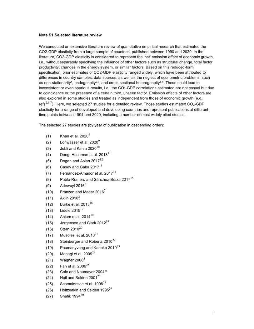
We conducted an extensive literature review of quantitative empirical research that estimated the CO2-GDP elasticity from a large sample of countries, published between 1990 and 2020. In the literature, CO2-GDP elasticity is considered to represent the 'net' emission effect of economic growth, i.e., without separately specifying the influence of other factors such as structural change, total factor productivity, changes in the energy system, or similar factors. Based on this reduced-form specification, prior estimates of CO2-GDP elasticity ranged widely, which have been attributed to differences in country samples, data sources, as well as the neglect of econometric problems, such as non-stationarity1, endogeneity2,3, and cross-sectional heterogeneity4,5. These could lead to inconsistent or even spurious results, i.e., the CO2-GDP correlations estimated are not casual but due to coincidence or the presence of a certain third, unseen factor. Emission effects of other factors are also explored in some studies and treated as independent from those of economic growth (e.g.,

refs2,6,7). Here, we selected 27 studies for a detailed review. Those studies estimated CO2-GDP

elasticity for a range of developed and developing countries and represent publications at different time points between 1994 and 2020, including a number of most widely cited studies. The selected 27 studies are (by year of publication in descending order):

(1) Khan et al. 20208

(2) Lohwasser et al. 20209

(3) Jebli and Kahia 202010

(4) Dong, Hochman et al. 201811

(5) Dogan and Aslan 201712

(6) Casey and Galor 201713

(7) Fernández-Amador et al. 201714

(8) Pablo-Romero and Sánchez-Braza 201715

(9) Adewuyi 20166

(10) Franzen and Mader 20167

(11) Aklin 20162

(12) Burke et al. 201516

(13) Liddle 201517

(14) Anjum et al. 201418

(15) Jorgenson and Clark 201219

(16) Stern 201020

(17) Musolesi et al. 201021

(18) Steinberger and Roberts 201022

(19) Poumanyvong and Kaneko 201023

(20) Managi et al. 200924

(21) Wagner 20085

(22) Fan et al. 200625

(23) Cole and Neumayer 200426

(24) Heil and Selden 200127

(25) Schmalensee et al. 199828

(26) Holtzeakin and Selden 199529

(27) Shafik 199430

2

Table S1 CO2-GDP elasticity estimates and empirical methods of the selected literature.

Dependent variable*

GDP per capita (GDP/p) or GDP*

Sample Econometric issues

addressed***

linear quadratic Time period Country/region NS E CD

(1) CO2 0.742 1990-2018 7 OECD countries Y Y Y

0.865 1990-2018 7 OECD countries Y Y Y

(2) CO2/p 0.282 1980–2014 84 countries Y N N

(3) CO2/p 2.398 −0.123 1980-2014 65 countries Y Y Y

(4) CO2/p 0.8413 1990-2014 3 North America

countries Y N Y

CO2/p 0.8362 1990-2014 22 South & Central America countries

Y N Y

CO2/p 0.8756 1990-2014 40 Europe and Eurasia

countries Y N Y

CO2/p 0.6820 1990-2014 14 Middle East countries Y N Y

CO2/p 0.8370 1990-2014 25 Africa countries Y N Y

CO2/p 0.7412 1990-2014 24 Asia Pacific countries Y N Y

CO2/p 0.7032 1990-2014 128 Global countries Y N Y

(5) CO2 -0.2 1995-2011 25 EU and candidate

countries Y N Y

(6) CO2/p 0.226 1950–2010 156 countries Y N N

(7) CO2/p 0.66 1997,2001,

2004,2007, 2011 66+12 region clusters N Y N

CO2/p** 0.786

(8)

CO2** 1.075 0.077 1995-2011 40 major economies Y N N

CO2/p** 1.147 0.083 1995-2011 40 major economies Y N N

CO2** 1.11 0.156 1995-2011 27 EU countries Y N N

CO2/p** 1.013 0.128 1995-2011 27 EU countries Y N N

CO2** 1.043 0.062 1995-2011 40 major economies Y N Y

1.016 0.05 1995-2011 40 major economies Y N Y

CO2/p** 0.997 0.042 1995-2011 40 major economies Y N Y

1.011 0.043 1995-2011 40 major economies Y N Y

CO2** 1.102 0.129 1995-2011 27 EU countries Y N Y

0.976 0.101 1995-2011 27 EU countries Y N Y

CO2/p** 0.963 0.088 1995-2011 27 EU countries Y N Y

0.953 0.073 1995-2011 27 EU countries Y N Y

(9) CO2/p 0.534 -0.035

1990-2015 40 top emitters (top 10

emitters per region) Y Y Y

1.093 -0.061

(10) CO2 0.76 -0.06

1970-2014 183 countries Y N N CO2/p 0.78

(11) CO2/p

0.155 0.002

1950-2000 151 countries N Y N 0.11 0.002

0.199 0.002

(12) CO2

0.52

1961-2010 189 countries Y Y N

0.65 1961-2010 OECD countries Y Y N

0.57 1961-2010 Non-OECD countries Y Y N

3

0.65 1961-2010 189 countries Y Y N

0.71 1961-2010 189 countries Y Y N

0.68 1961-2010 189 countries Y Y N

(13)

CO2/p 0.57 1971-2011 26 OECD countries Y N Y

CO2/p 0.75 1971-2011 26 OECD countries Y N Y

CO2/p 0.97 1971-2011 54 Non-OECD countries Y N Y

CO2/p 0.96 1971-2011 54 Non-OECD countries Y N Y

CO2 0.81 1971-2011 All (26+54) Y N Y

CO2 0.87 1971-2011 All (26+54) Y N Y

CO2 0.58 1971-2011 26 OECD countries Y N Y

CO2 0.71 1971-2011 26 OECD countries Y N Y

CO2 0.89 1971-2011 54 Non-OECD countries

54 Non-OECD countries

Y N Y

CO2 0.83 1971-2011 Y N Y

(14) CO2/p 0.9147

1971-2010 134 countries

Y Y N 0.9074 97 countries

(15)

CO2 1.023 1960-2005 86 (DC+LDC) countries Y N N

CO2 0.986 1960-2005 22 DC countries Y N N

CO2 1.003 1960-2005 64 LDC countries Y N N

CO2/p 0.467 1960-2005 86 (DC+LDC) countries Y N N

CO2/p 0.757 1960-2005 22 DC countries Y N N

CO2/p 0.388 1960-2005 64 LDC countries Y N N

(16) CO2/p 1.612 1960-2000 24 OECD countries

Y N N 1.509 1950-2000 100 countries countries

(17) CO2/p

1.96 0.08 1959-2001 109 countries Y N Yd

10.91 0.56 1959-2001 G7 countries Y N Yd

10.76 0.56 1959-2001 EU15 countries Y N Yd

8.91 0.45 1959-2001 OECD countries Y N Yd

0.29 0.04 1959-2001 Non-OECD countries Y N Yd

0.16 0.02 1959-2001 40 poorest countries Y N Yd

(18) CO2/p

0.687 1975 85 countries -- N N

0.688 1980 85 countries -- N N

0.662 1985 85 countries -- N N

0.666 1990 85 countries -- N N

0.702 1995 85 countries -- N N

0.741 2000 85 countries -- N N

0.722 2005 85 countries -- N N

(19) CO2

0.376 1975-2005 99 countries Y N N

2.498 1975-2005 23 low-income countries Y N N

0.987 1975-2005 43 middle-income

countries Y N N

0.829 1975-2005 33 high-income countries Y N N

(20) CO2/p 0.84 -0.42 1973-2000 88 countries N Y N

(21) CO2/p 0.731 0.202

1950-2000 100 countries Y Y Y 0.589 0.290

(22) CO2

0.68 1975-2000 208 countries N N N

0.57 1975-2000 55 high-income N N N

0.33 1975-2000 40 upper-middle income N N N

0.44 1975-2000 54 lower-middle income N N N

0.26 1975-2000 59 low-income N N N

(23) CO2 0.892 1975-1998 86 countries Y N N

4

(24) CO2/p 0.4083 0.1428 1950-1992 132 countries N N N

(25) CO2/p

-0.28 1950-1990 income: $200-629/year N N N

0.31 1950-1990 income: $629-932/year N N N

1.29 1950-1990 income: $932-1283/year N N N

0.79 1950-1990 income: $1283-

1728/year N N N

1.1 1950-1990 income: $1728-

2352/year N N N

0.66 1950-1990 income: $2352-

3190/year N N N

0.54 1950-1990 income: $3190-

4467/year N N N

0.71 1950-1990 income: $4467-

6598/year N N N

0.07(e) 1950-1990 income: $6598-

9799/year N N N

-0.3 1950-1990 income: $9799-

19627/year N N N

(26) CO2/p 0.5204 1951-1986 130 countries N N N

(27) CO2/p 1.62 1960-1989 153 countries N N N

*: Data sources of CO2 and GDP (more details about the data sources can be found in the referenced articles):

(1) CO2 emissions from the use of fossil fuels, cement manufacturing, and consumption of gas, solid, and liquid fuels, as well as gas flaring: The World Bank31; real GDP at constant 2005 national prices: PWT32,33.

(2) Total CO2 emissions from fossil fuel combustion: CDIAC34; per capita GDP in constant 2011 US$: PWT32,33.

(3) CO2 emissions (no further specification) and GDP (constant 2010 USD): The World Bank31. (4) CO2 emissions (no further specification) and GDP (constant 2010 US$): The World Bank31. (5) CO2 emissions (no further specification) and GDP (constant 2005 US$): The World Bank31. (6) CO2 emissions from fossil fuel combustion: CDIAC34; per capita GDP: output-side measure of

income per capita: PWT 8.032,33 (7) CO2 from fossil fuel combustion: GTAP35; GDP in constant PPP: The World Bank8. (8) CO2 from fossil fuel combustion, cement, minerals, refineries and GDP in constant 1995 US$:

WIOD36. (9) CO2 from fossil fuel combustion and cement production, excluding other emissions such as

from land use change and forestry: CDIAC34; GDP: PWT32,33 or The World Bank31. (10) CO2 from fossil fuel use and industrial processes (cement production, carbonate use of

limestone and dolomite, non-energy use of fuels and other combustion), excluding short-cycle biomass burning (such as agricultural waste burning) and large-scale biomass burning (such as forest fires: EDGAR37; GDP PPP: IMF38.

(11) CO2 from fossil fuel consumption and cement production: CDIAC34; GDP: The World Bank31. (12) CO2 from fossil fuel combustion and cement production, excluding other emissions such as

from land use change and forestry: CDIAC34; GDP in constant 2005 US$: The World Bank31, (13) CO2 from fossil fuel combustion: International Energy Agency (IEA, no further specification);

real GDP (unknown source). (14) CO2 from combustion of fossil fuels, gas flaring, and cement production: CDIAC39; GDP growth

rates, GDP level: PWT32,33. (15) CO2 from fossil fuel combustion, gas flaring, and cement manufacturing, excluding emissions

from land use change or bunker fuels used in international transportation: CAIT40 which compiles data from CDIAC, IEA, and EIA; GDP in constant 2000 US$: The World Bank31.

(16) CO2 from fossil fuel combustion and cement production, excluding other emissions such as from land use change and forestry: CDIAC34; real GDP per capita: Maddison Project41.

(17) CO2 from combustion of fossil fuels, gas flaring, and cement production: CDIAC34; GDP in 1990 International 'Geary-Khamis' dollars: Maddison Project41.

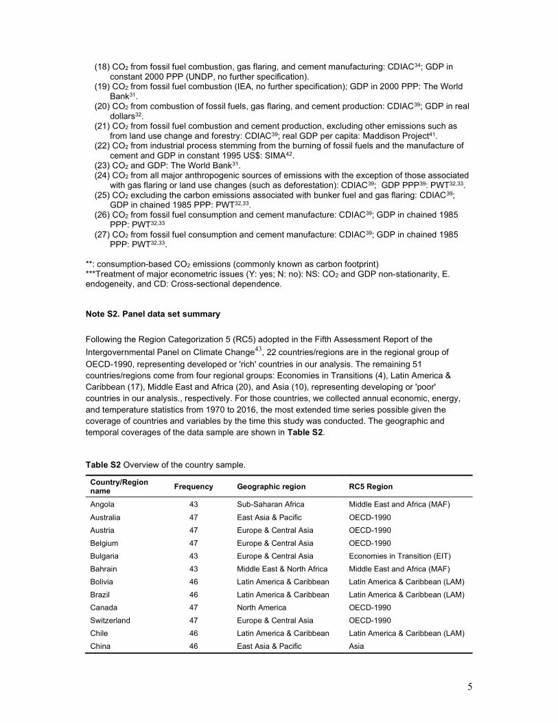
5

(18) CO2 from fossil fuel combustion, gas flaring, and cement manufacturing: CDIAC34; GDP in constant 2000 PPP (UNDP, no further specification).

(19) CO2 from fossil fuel combustion (IEA, no further specification); GDP in 2000 PPP: The World Bank31.

(20) CO2 from combustion of fossil fuels, gas flaring, and cement production: CDIAC39; GDP in real dollars32.

(21) CO2 from fossil fuel combustion and cement production, excluding other emissions such as from land use change and forestry: CDIAC39; real GDP per capita: Maddison Project41.

(22) CO2 from industrial process stemming from the burning of fossil fuels and the manufacture of cement and GDP in constant 1995 US$: SIMA42.

(23) CO2 and GDP: The World Bank31. (24) CO2 from all major anthropogenic sources of emissions with the exception of those associated

with gas flaring or land use changes (such as deforestation): CDIAC39; GDP PPP39: PWT32,33. (25) CO2 excluding the carbon emissions associated with bunker fuel and gas flaring: CDIAC39;

GDP in chained 1985 PPP: PWT32,33. (26) CO2 from fossil fuel consumption and cement manufacture: CDIAC39; GDP in chained 1985

PPP: PWT32,33 (27) CO2 from fossil fuel consumption and cement manufacture: CDIAC39; GDP in chained 1985

PPP: PWT32,33.

**: consumption-based CO2 emissions (commonly known as carbon footprint) ***Treatment of major econometric issues (Y: yes; N: no): NS: CO2 and GDP non-stationarity, E. endogeneity, and CD: Cross-sectional dependence.

Note S2. Panel data set summary

Following the Region Categorization 5 (RC5) adopted in the Fifth Assessment Report of the

Intergovernmental Panel on Climate Change43, 22 countries/regions are in the regional group of

OECD-1990, representing developed or 'rich' countries in our analysis. The remaining 51 countries/regions come from four regional groups: Economies in Transitions (4), Latin America & Caribbean (17), Middle East and Africa (20), and Asia (10), representing developing or 'poor' countries in our analysis., respectively. For those countries, we collected annual economic, energy, and temperature statistics from 1970 to 2016, the most extended time series possible given the coverage of countries and variables by the time this study was conducted. The geographic and temporal coverages of the data sample are shown in Table S2. Table S2 Overview of the country sample.

Country/Region name

Frequency Geographic region RC5 Region

Angola 43 Sub-Saharan Africa Middle East and Africa (MAF)

Australia 47 East Asia & Pacific OECD-1990

Austria 47 Europe & Central Asia OECD-1990

Belgium 47 Europe & Central Asia OECD-1990

Bulgaria 43 Europe & Central Asia Economies in Transition (EIT)

Bahrain 43 Middle East & North Africa Middle East and Africa (MAF)

Bolivia 46 Latin America & Caribbean Latin America & Caribbean (LAM)

Brazil 46 Latin America & Caribbean Latin America & Caribbean (LAM)

Canada 47 North America OECD-1990

Switzerland 47 Europe & Central Asia OECD-1990

Chile 46 Latin America & Caribbean Latin America & Caribbean (LAM)

China 46 East Asia & Pacific Asia

6

Côte d'Ivoire 46 Sub-Saharan Africa Middle East and Africa (MAF)

Cameroon 46 Sub-Saharan Africa Middle East and Africa (MAF)

Colombia 46 Latin America & Caribbean Latin America & Caribbean (LAM)

Costa Rica 46 Latin America & Caribbean Latin America & Caribbean (LAM)

Germany 47 Europe & Central Asia OECD-1990

Denmark 47 Europe & Central Asia OECD-1990

Dominican Republic

46 Latin America & Caribbean Latin America & Caribbean (LAM)

Ecuador 46 Latin America & Caribbean Latin America & Caribbean (LAM)

Egypt 46 Middle East & North Africa Middle East and Africa (MAF)

Spain 47 Europe & Central Asia OECD-1990

Finland 47 Europe & Central Asia OECD-1990

France 47 Europe & Central Asia OECD-1990

United Kingdom 47 Europe & Central Asia OECD-1990

Greece 47 Europe & Central Asia OECD-1990

Guatemala 46 Latin America & Caribbean Latin America & Caribbean (LAM)

Hong Kong 46 East Asia & Pacific Asia

Honduras 46 Latin America & Caribbean Latin America & Caribbean (LAM)

Hungary 43 Europe & Central Asia Economies in Transition (EIT)

Indonesia 46 East Asia & Pacific Asia

India 46 South Asia Asia

Ireland 47 Europe & Central Asia OECD-1990

Iran 46 Middle East & North Africa Middle East and Africa (MAF)

Israel 46 Middle East & North Africa Middle East and Africa (MAF)

Italy 47 Europe & Central Asia OECD-1990

Jamaica 46 Latin America & Caribbean Latin America & Caribbean (LAM)

Jordan 46 Middle East & North Africa Middle East and Africa (MAF)

Japan 47 East Asia & Pacific OECD-1990

Kenya 46 Sub-Saharan Africa Middle East and Africa (MAF)

Republic of Korea

46 East Asia & Pacific Asia

Kuwait 43 Middle East & North Africa Middle East and Africa (MAF)

Sri Lanka 46 South Asia Asia

Morocco 46 Middle East & North Africa Middle East and Africa (MAF)

Mexico 46 Latin America & Caribbean Latin America & Caribbean (LAM)

Mozambique 46 Sub-Saharan Africa Middle East and Africa (MAF)

Malaysia 46 East Asia & Pacific Asia

Nigeria 46 Sub-Saharan Africa Middle East and Africa (MAF)

Netherlands 47 Europe & Central Asia OECD-1990

Norway 47 Europe & Central Asia OECD-1990

New Zealand 47 East Asia & Pacific OECD-1990

Panama 46 Latin America & Caribbean Latin America & Caribbean (LAM)

Peru 46 Latin America & Caribbean Latin America & Caribbean (LAM)

Philippines 46 East Asia & Pacific Asia

Poland 43 Europe & Central Asia Economies in Transition (EIT)

Portugal 47 Europe & Central Asia OECD-1990

Paraguay 46 Latin America & Caribbean Latin America & Caribbean (LAM)

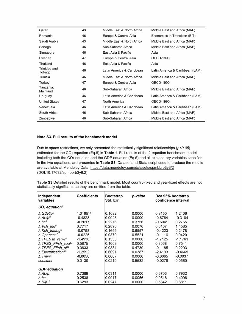
7

Qatar 43 Middle East & North Africa Middle East and Africa (MAF)

Romania 46 Europe & Central Asia Economies in Transition (EIT)

Saudi Arabia 43 Middle East & North Africa Middle East and Africa (MAF)

Senegal 46 Sub-Saharan Africa Middle East and Africa (MAF)

Singapore 46 East Asia & Pacific Asia

Sweden 47 Europe & Central Asia OECD-1990

Thailand 46 East Asia & Pacific Asia

Trinidad and Tobago

46 Latin America & Caribbean Latin America & Caribbean (LAM)

Tunisia 46 Middle East & North Africa Middle East and Africa (MAF)

Turkey 47 Europe & Central Asia OECD-1990

Tanzania: Mainland

46 Sub-Saharan Africa Middle East and Africa (MAF)

Uruguay 46 Latin America & Caribbean Latin America & Caribbean (LAM)

United States 47 North America OECD-1990

Venezuela 46 Latin America & Caribbean Latin America & Caribbean (LAM)

South Africa 46 Sub-Saharan Africa Middle East and Africa (MAF)

Zimbabwe 46 Sub-Saharan Africa Middle East and Africa (MAF)

Note S3. Full results of the benchmark model

Due to space restrictions, we only presented the statistically significant relationships (p<0.05) estimated for the CO2 equation (Eq.6) in Table 1. Full results of the 2-equation benchmark model, including both the CO2 equation and the GDP equation (Eq.5) and all explanatory variables specified in the two equations, are presented in Table S3. Dataset and Stata script used to produce the results are available at Mendeley Data: https://data.mendeley.com/datasets/spmbbrb3y6/2 (DOI:10.17632/spmbbrb3y6.2). Table S3 Detailed results of the benchmark model. Most country-fixed and year-fixed effects are not statistically significant, so they are omitted from the table.

Independent variables

Coefficients Bootstrap Std. Err.

p-value Bca 95% bootstrap confidence interval

CO2 equation1

∆ GDP/p2 1.019513 0.1082 0.0000 0.8150 1.2406 ∆ AL/p3 -0.4823 0.0923 0.0000 -0.6764 -0.3184 ∆ hc4 -0.2017 0.2276 0.3756 -0.6041 0.2765 ∆ Vsh_Ind5 0.7717 0.2890 0.0076 0.3107 1.4585 ∆ Ksh_Intang6 -0.0758 0.1699 0.6557 -0.4223 0.2478 ∆ Openess7 -0.0225 0.0379 0.5521 -0.1116 0.0420 ∆ TPESsh_renw8 -1.4936 0.1333 0.0000 -1.7125 -1.1761 ∆ TPES_FFsh_coal9 0.5875 0.1063 0.0000 0.3568 0.7541 ∆ TPES_FFsh_oil9 0.0633 0.0884 0.4739 -0.1185 0.2203 ∆ Electrification10 -1.2592 0.6091 0.0387 -2.4193 -0.4669 ∆ Tmin11 -0.0050 0.0007 0.0000 -0.0065 -0.0037 constant 0.0130 0.0219 0.5532 -0.0279 0.0560 GDP equation

∆ AL/p 0.7389 0.0311 0.0000 0.6703 0.7932 ∆ hc 0.2538 0.0917 0.0056 0.0518 0.4096 ∆ K/p12 0.6293 0.0247 0.0000 0.5842 0.6811

8

constant -0.0058 0.0089 0.5160 -0.0263 0.0089

1. The dependent variable is ∆CO2/p, i.e. annual changes of per capita carbon dioxide emissions related to fossil fuel combustion and industrial processes, obtained from IEA44; p: total population; "pop" in PWT 9.132; ∆ is the first difference operator;

2. GDP/p: per capita real gross domestic product at constant U.S. dollars; GDP and p are estimated as "rgdpna" and 'pop' in PWT 9.132;

3. AL/p: labor augmented productivity (A∙L) adjusted for population (p); labor (L, the number of people engaged in employment), total factor productivity (A), and population (p) are estimated as "emp", 'rtfpna', and 'pop' in PWT 9.132

4. hc: human capital index, "hc" in PWT 9.132

5. Vsh_Ind: share of total value added by industrial sectors (ISIC G-P)45;

6. Ksh_Intang: share of intangible assets in capital stock, "Ksh_Other" in PWT 9.132;

7. Openness: international trade openness, the fraction of value added contributed by trade (import plus export)45;

8. TPESsh_renw: share of renewables in total primary energy supply (TPES)44

9. TPES_FFsh_coal, TPES_FFsh_oil: Share of coal & coal products and oil & oil products in fossil primary energy supply, respectively44;

10. Electrification: fraction of electricity in final energy consumption44;

11. Tmin: the lowest monthly temperature each year46;

12. K/p: per capita capital stock, capital stock and population are estimated as "rnna" and 'pop' in PWT 9.132;

13. test estimated coefficient =1: p-value = 0.8052, i.e., fail to reject the coefficient = 1.

Note S4. Testing alternative model specifications

We estimated alternative models using various model specifications to test the robustness of our benchmark model and main findings. Those models explored various specifications of growth-related effects (Table S4) and an extension to a three-equation model by adding an energy equation to bridge the CO2 and GDP equations (Table S5). Given that some discrepancies of previous CO2-GDP estimates were attributed to the data sources of CO2 and GDP, we also collected and used different CO2 and GDP estimates in our benchmark model to test the robustness of our main findings (Tables S7). Furthermore, our use of the first differenced annual time series may be vulnerable to the influences of cyclical variations. We thus tested the effects by taking and using 5-year averages of the variables in the benchmark model (Table S7). Overall, the results show that our benchmark model and main findings are robust to alternative model specifications and data sources. Table S4: Results of various model specifications for growth-related effects. (1) adding 1-year lag of GDP growth rate to the CO2 equation; (2) adding 1-year and 2-year lags of GDP growth rate to the CO2 equation; (3) adding 1-year, 2-year, and 3-year lags of GDP growth rate to the CO2 equation; (4) testing for asymmetric effects: GDP expansion vs. GDP recession in the CO2 equation (5) testing the effects of income levels on the CO2-GDP elasticity; (6) adding trade activities to the GDP equation; (7) alternative GDP equation specification: Y = f(A,L,K,H); (8) replacing hc with yr_sch (average years of

schooling in the population aged 25 years and older) obtained from47.

Independent variables Benchmark (1) (2) (3) (4) (5) (6) (7) (8)

CO2 equation

∆ GDP/pa 1.0195*** 0.9655*** 0.9505*** 0.9461*** 1.0292*** 1.0209*** 1.0206*** 0.9694*** 0.9989*** ∆ AL/p -0.4823*** -0.4504*** -0.4378*** -0.4294*** -0.4824*** -0.4830*** -0.4826*** -0.3796*** ∆ A -0.5025*** ∆ L/p -0.2505*** ∆ hc -0.2017 -0.1914 -0.1736 -0.1831 -0.1980 -0.2015 -0.2009 -0.2517

9

∆ yr_sch -0.0972 ∆ Vsh_Ind 0.7717*** 0.7840*** 0.7923*** 0.7811*** 0.7686*** 0.7750*** 0.7752*** 0.7853*** 0.7548*** ∆ Ksh_Intang -0.0758 -0.0841 -0.0689 -0.0894 -0.0759 -0.0757 -0.0757 -0.0853 -0.0916 ∆ Openess -0.0225^ -0.0238^ -0.0229^ -0.0242^ -0.0218 -0.0224^ -0.0211 -0.0233^ -0.0240^ ∆ TPESsh_renw -1.4936*** -1.4927*** -1.4823*** -1.4787*** -1.4940*** -1.4941*** -1.4941*** -1.4953*** -1.4902*** ∆ TPES_FFsh_coal 0.5875*** 0.5908*** 0.5913*** 0.5945*** 0.5877*** 0.5875*** 0.5875*** 0.5872*** 0.5875*** ∆ TPES_FFsh_oil 0.0633 0.0640 0.0643 0.0651 0.0634 0.0633 0.0633 0.0617 0.0640 ∆ Electrification -1.2592*** -1.2669*** -1.2662*** -1.2494*** -1.2588*** -1.2599*** -1.2599*** -1.2590*** -1.2537*** ∆ Tmin -0.0050*** -0.0050*** -0.0050*** -0.0050*** -0.0049*** -0.0050*** -0.0050*** -0.0050*** -0.0050*** ∆ LP -0.0011 -0.0011 -0.0011 -0.0010 -0.0011 -0.0011 -0.0011 -0.0011 -0.0011 ∆ GDP/pt-1 (1-yr lag) 0.0460^ 0.0461 0.0411

∆ GDP/pt-2 (2-yr lag) 0.0213 0.0264

∆ GDP/pt-3 (3-yr lag) -0.0119

∆ GDP/p+ (expansion) 0.0099

∆ GDP/p- (recession) 0.0119

Developed # ∆ GDP/p -0.0072 -0.0072

constant 0.0130 0.0124 0.0122 0.0123 0.0031 0.0130 0.0130

GDP equation

∆ AL/p 0.7389*** 0.7387*** 0.7383*** 0.7376*** 0.7389*** 0.7389*** 0.7386*** 0.7406*** ∆ A 0.8230***

∆ L/p 0.4395*** ∆ hc 0.2538*** 0.2541*** 0.2572*** 0.2424*** 0.2538*** 0.2538*** 0.2529*** 0.3485*** ∆ yr_sch 0.1343*** ∆ K/p 0.6293*** 0.6303*** 0.6336*** 0.6347*** 0.6293*** 0.6293*** 0.6296*** 0.6766*** 0.6294*** ∆ O -0.0025

constant -0.0058 -0.0058 -0.0058 -0.0057 -0.0058 -0.0058 -0.0058

N 3283 3261 3196 3131 3283 3283 3283 3283 3283

a. All estimates CO2-GDP elasticity are not statistically different from 1 (p<0.001).; b. ^p<0.10, * p<0.05, ** p<0.01, *** p<0.001

Table S5: Results from the three-equation model, adding an equation for primary energy supply. Using primary energy supply to bridge GDP and CO2, we can further elucidate the emission reduction mechanisms, i.e. whether by affecting primary energy use or the emission intensity of energy supplies or emissions from industrial processes. Those nuances are discussed in the main manuscript.

CO2 equation Energy equation GDP equation

∆ TPES/pa 0.9827***b ∆ GDP/p 0.9348*** ∆ AL/p 0.7389*** ∆ Vsh_Ind 0.1537* ∆ AL/p -0.4063*** ∆ hc 0.2539*** ∆ Ksh_Intang -0.1134 ∆ hc -0.1418 ∆ K/p 0.6290*** ∆ Openessc 0.0327** ∆ Vsh_Ind 0.6373*** constant -0.0058 ∆ TPESsh_renw -0.9986*** ∆ Ksh_Intang 0.0498

∆ TPES_FFsh_coal 0.4274*** ∆ Openessc -0.0582***

∆ TPES_FFsh_oil 0.0030 ∆ TPESsh_renw -0.5422***

∆ Electrification -0.0020 ∆ TPES_FFsh_coal 0.1512*

∆ LP 0.0002 ∆ TPES_FFsh_oil 0.0734^ -0.0000 ∆ Electrification -1.2956*** ∆ Tmin -0.0041*** ∆ LP 0.0004 constant -0.0035

N 3283

a. Indirectly, we can derive a proportional CO2-GDP elasticity, the same as using the two-equation benchmark, b. ^p<0.10, * p<0.05, ** p<0.01, *** p<0.001. c. Trade openness (or globalization) appears to reduce a country's emissions by reducing its primary energy supply while increase the emissions by increasing the carbon intensity of the energy supply or the emissions from industrial processes. The two opposite emission effects cancel each other out.

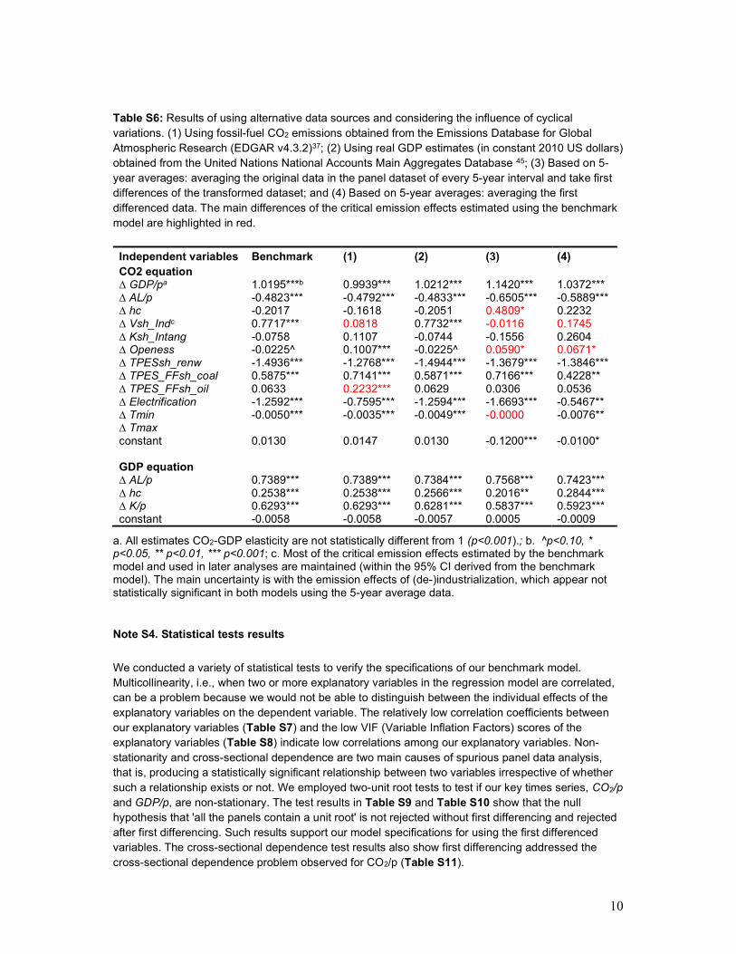
10

Table S6: Results of using alternative data sources and considering the influence of cyclical variations. (1) Using fossil-fuel CO2 emissions obtained from the Emissions Database for Global Atmospheric Research (EDGAR v4.3.2)37; (2) Using real GDP estimates (in constant 2010 US dollars) obtained from the United Nations National Accounts Main Aggregates Database 45; (3) Based on 5-year averages: averaging the original data in the panel dataset of every 5-year interval and take first differences of the transformed dataset; and (4) Based on 5-year averages: averaging the first differenced data. The main differences of the critical emission effects estimated using the benchmark model are highlighted in red.

Independent variables Benchmark (1) (2) (3) (4) CO2 equation

∆ GDP/pa 1.0195***b 0.9939*** 1.0212*** 1.1420*** 1.0372*** ∆ AL/p -0.4823*** -0.4792*** -0.4833*** -0.6505*** -0.5889*** ∆ hc -0.2017 -0.1618 -0.2051 0.4809* 0.2232 ∆ Vsh_Indc 0.7717*** 0.0818 0.7732*** -0.0116 0.1745 ∆ Ksh_Intang -0.0758 0.1107 -0.0744 -0.1556 0.2604 ∆ Openess -0.0225^ 0.1007*** -0.0225^ 0.0590* 0.0671* ∆ TPESsh_renw -1.4936*** -1.2768*** -1.4944*** -1.3679*** -1.3846*** ∆ TPES_FFsh_coal 0.5875*** 0.7141*** 0.5871*** 0.7166*** 0.4228** ∆ TPES_FFsh_oil 0.0633 0.2232*** 0.0629 0.0306 0.0536 ∆ Electrification -1.2592*** -0.7595*** -1.2594*** -1.6693*** -0.5467** ∆ Tmin -0.0050*** -0.0035*** -0.0049*** -0.0000 -0.0076** ∆ Tmax constant 0.0130 0.0147 0.0130 -0.1200*** -0.0100* GDP equation

∆ AL/p 0.7389*** 0.7389*** 0.7384*** 0.7568*** 0.7423*** ∆ hc 0.2538*** 0.2538*** 0.2566*** 0.2016** 0.2844*** ∆ K/p 0.6293*** 0.6293*** 0.6281*** 0.5837*** 0.5923*** constant -0.0058 -0.0058 -0.0057 0.0005 -0.0009

a. All estimates CO2-GDP elasticity are not statistically different from 1 (p<0.001).; b. ^p<0.10, * p<0.05, ** p<0.01, *** p<0.001; c. Most of the critical emission effects estimated by the benchmark model and used in later analyses are maintained (within the 95% CI derived from the benchmark model). The main uncertainty is with the emission effects of (de-)industrialization, which appear not statistically significant in both models using the 5-year average data.

Note S4. Statistical tests results

We conducted a variety of statistical tests to verify the specifications of our benchmark model. Multicollinearity, i.e., when two or more explanatory variables in the regression model are correlated, can be a problem because we would not be able to distinguish between the individual effects of the explanatory variables on the dependent variable. The relatively low correlation coefficients between our explanatory variables (Table S7) and the low VIF (Variable Inflation Factors) scores of the explanatory variables (Table S8) indicate low correlations among our explanatory variables. Non-stationarity and cross-sectional dependence are two main causes of spurious panel data analysis, that is, producing a statistically significant relationship between two variables irrespective of whether such a relationship exists or not. We employed two-unit root tests to test if our key times series, CO2/p and GDP/p, are non-stationary. The test results in Table S9 and Table S10 show that the null hypothesis that 'all the panels contain a unit root' is not rejected without first differencing and rejected after first differencing. Such results support our model specifications for using the first differenced variables. The cross-sectional dependence test results also show first differencing addressed the cross-sectional dependence problem observed for CO2/p (Table S11).

11

Table S7: Correlation coefficients among all variables used in the benchmark model (∆: the first difference operator).

0 1 2 3 4 5 6 7 8 9 10 11 12

0 ∆ CO2/p 1.00

1 ∆ GDP/p 0.40 1.00

2 ∆ K/p 0.22 0.37 1.00

3 ∆ AL/p 0.27 0.82 0.00 1.00

4 ∆ HC 0.09 0.02 0.07 -0.05 1.00

5 ∆ Ksh_Intang -0.03 -0.03 0.03 -0.04 0.01 1.00

6 ∆ Vsh_Ind 0.31 0.46 0.07 0.39 0.00 -0.04 1.00

7 ∆ Openness -0.04 0.00 0.03 -0.02 -0.02 0.01 -0.09 1.00

8 ∆ TPESsh_renw -0.45 -0.12 -0.08 -0.07 -0.05 0.01 -0.04 -0.01 1.00

9 ∆ TPES_FFsh_coal 0.12 -0.01 -0.01 -0.01 0.05 -0.02 0.00 0.03 -0.03 1.00

10 ∆ TPES_FFsh_oil -0.12 -0.09 0.00 -0.07 -0.03 -0.01 -0.17 0.05 0.04 -0.53 1.00

11 ∆ Electrification -0.23 -0.06 0.07 -0.07 0.04 0.02 -0.08 0.10 0.01 0.08 -0.01 1.00

12 ∆ Tmin -0.13 0.00 0.01 0.00 0.00 0.02 0.00 0.01 0.05 -0.06 0.05 0.06 1.00

Table S8: Results of multicollinearity tests for the benchmark model. Multicollinearity can be detected via various methods. Here, we employ the most common one – VIF (Variable Inflation Factors). VIF score of an independent variable represents how well the variable is explained by other independent variables. As a rule of thumb, a variable whose VIF values are greater than 10 may merit further investigation. The maximum VIF value of all variables is 3.46, considerably lower than 10.

Equation (6) Equation (5)

Variable VIFa Variable VIF ∆ GDP/p 3.46 ∆ AL/p 1.11 ∆ AL/p 3.12 ∆ hc 1.49 ∆ hc 1.47 ∆ K/p 1.79 ∆ Vsh_Ind 1.36 ∆ Ksh_Intang 1.08 ∆ Ksh_Intang 1.08

∆ Openess 1.13

∆ TPESsh_renw 1.09

∆ TPES_FFsh_coal 1.66

∆ TPES_FFsh_oil 1.62

∆ Electrification 1.05

∆ Tmin 1.09

∆ Tmax 1.20

Table S9: Results of the unit-root test using the Im-Pesaran-Shin tests48 on per capita CO2, GDP, and total primary energy supply (TPES) before and after first differencing. Ho: All panels contain unit roots, Ha: Some panels are stationary.

CO2/p TPES/p GDP/p Statistic p-value Statistic p-value Statistic p-value t-bar -1.5751 -1.6794 -0.999 -5.04 t-tilde-bar -1.4563 -1.572 -0.9315 Z-t-tilde-bar 0.1645 0.5653 -1.055 0.1457 5.7394 1 ∆CO2/p ∆TPES/p ∆GDP/p Statistic p-value Statistic p-value Statistic p-value

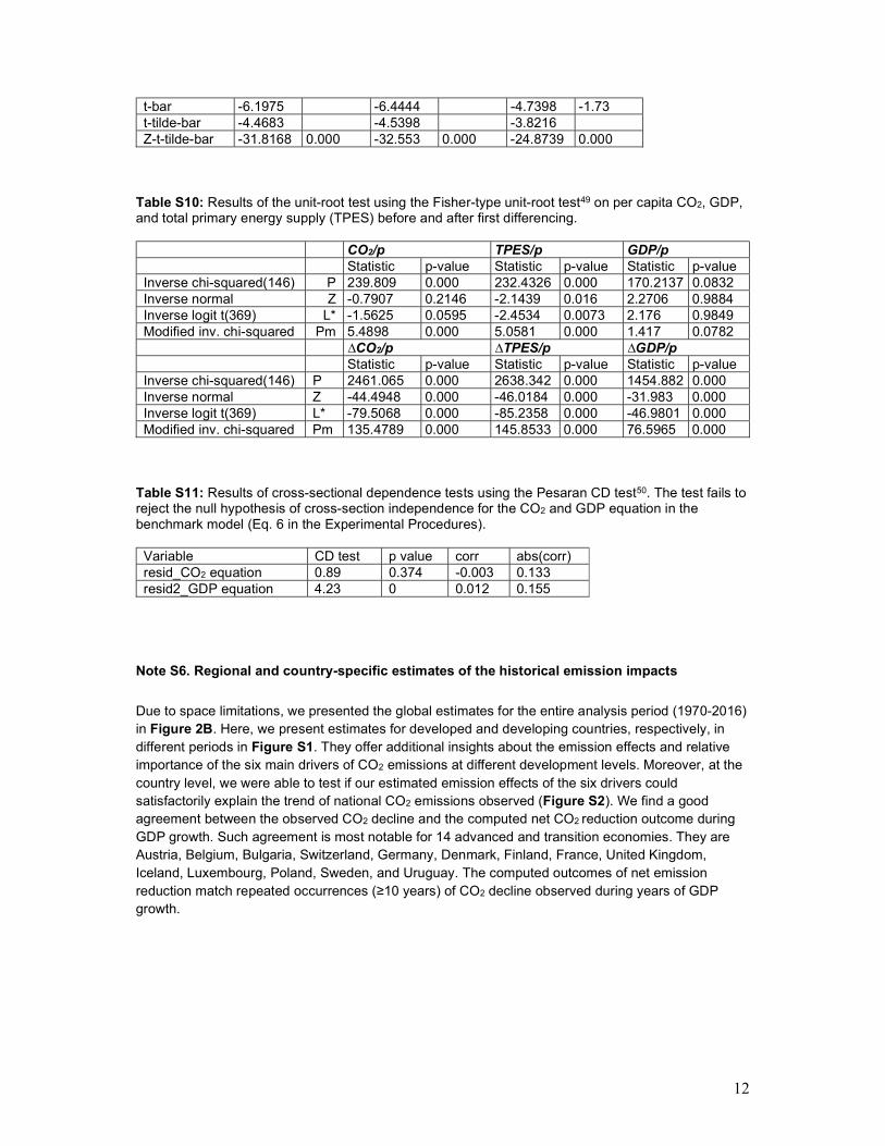
12

t-bar -6.1975 -6.4444 -4.7398 -1.73 t-tilde-bar -4.4683 -4.5398 -3.8216 Z-t-tilde-bar -31.8168 0.000 -32.553 0.000 -24.8739 0.000

Table S10: Results of the unit-root test using the Fisher-type unit-root test49 on per capita CO2, GDP, and total primary energy supply (TPES) before and after first differencing.

CO2/p TPES/p GDP/p Statistic p-value Statistic p-value Statistic p-value Inverse chi-squared(146) P 239.809 0.000 232.4326 0.000 170.2137 0.0832 Inverse normal Z -0.7907 0.2146 -2.1439 0.016 2.2706 0.9884 Inverse logit t(369) L* -1.5625 0.0595 -2.4534 0.0073 2.176 0.9849 Modified inv. chi-squared Pm 5.4898 0.000 5.0581 0.000 1.417 0.0782 ∆CO2/p ∆TPES/p ∆GDP/p Statistic p-value Statistic p-value Statistic p-value Inverse chi-squared(146) P 2461.065 0.000 2638.342 0.000 1454.882 0.000 Inverse normal Z -44.4948 0.000 -46.0184 0.000 -31.983 0.000 Inverse logit t(369) L* -79.5068 0.000 -85.2358 0.000 -46.9801 0.000 Modified inv. chi-squared Pm 135.4789 0.000 145.8533 0.000 76.5965 0.000

Table S11: Results of cross-sectional dependence tests using the Pesaran CD test50. The test fails to reject the null hypothesis of cross-section independence for the CO2 and GDP equation in the benchmark model (Eq. 6 in the Experimental Procedures).

Variable CD test p value corr abs(corr) resid_CO2 equation 0.89 0.374 -0.003 0.133 resid2_GDP equation 4.23 0 0.012 0.155

Note S6. Regional and country-specific estimates of the historical emission impacts

Due to space limitations, we presented the global estimates for the entire analysis period (1970-2016) in Figure 2B. Here, we present estimates for developed and developing countries, respectively, in different periods in Figure S1. They offer additional insights about the emission effects and relative importance of the six main drivers of CO2 emissions at different development levels. Moreover, at the country level, we were able to test if our estimated emission effects of the six drivers could satisfactorily explain the trend of national CO2 emissions observed (Figure S2). We find a good agreement between the observed CO2 decline and the computed net CO2 reduction outcome during GDP growth. Such agreement is most notable for 14 advanced and transition economies. They are Austria, Belgium, Bulgaria, Switzerland, Germany, Denmark, Finland, France, United Kingdom, Iceland, Luxembourg, Poland, Sweden, and Uruguay. The computed outcomes of net emission reduction match repeated occurrences (≥10 years) of CO2 decline observed during years of GDP growth.

13

Figure S1: Total contributions to emission changes by region and decade. Error bars show the ranges calculated from the 95% bias-corrected and accelerated (BCa) confidence intervals. Main driving forces of CO2 emissions: economic growth rate (1), economic productivity (2), deindustrialization (3), decarbonization by shifting to renewables (4) or from coal to natural gas (5), electrification (6), and winter warming (7).

14

Economic

productivity rise

De-industrialization

Energy system decarbonization

Electrification Winter warming

Country-fixed effects

Figure S2 Observed and computed desirable trends for 16 countries where occurrences of CO2 per capita decline were observed during GDP per capita growth repeatedly (≥15 years). Quantities of CO2 (denoted by '∙') and GDP (marked by 'x') are normalized to 1 in the year 1971. “Circles” indicate CO2 reduction was observed during GDP growth; "Colored circles" illustrate that the computed results show CO2 emission reduction in the same year - Color indicates the dominant emission reduction force.

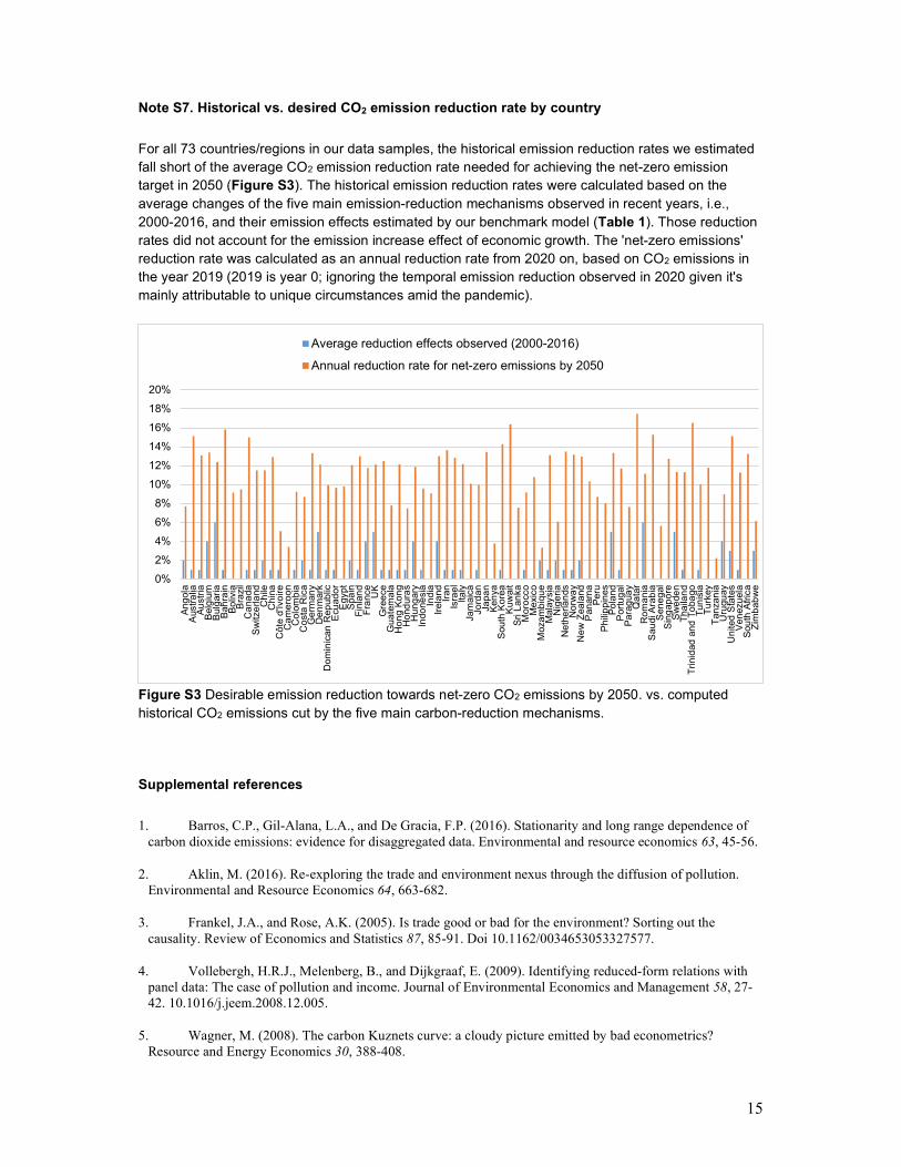
15

Note S7. Historical vs. desired CO2 emission reduction rate by country

For all 73 countries/regions in our data samples, the historical emission reduction rates we estimated fall short of the average CO2 emission reduction rate needed for achieving the net-zero emission target in 2050 (Figure S3). The historical emission reduction rates were calculated based on the average changes of the five main emission-reduction mechanisms observed in recent years, i.e., 2000-2016, and their emission effects estimated by our benchmark model (Table 1). Those reduction rates did not account for the emission increase effect of economic growth. The 'net-zero emissions' reduction rate was calculated as an annual reduction rate from 2020 on, based on CO2 emissions in the year 2019 (2019 is year 0; ignoring the temporal emission reduction observed in 2020 given it's mainly attributable to unique circumstances amid the pandemic).

Figure S3 Desirable emission reduction towards net-zero CO2 emissions by 2050. vs. computed historical CO2 emissions cut by the five main carbon-reduction mechanisms.

Supplemental references

1. Barros, C.P., Gil-Alana, L.A., and De Gracia, F.P. (2016). Stationarity and long range dependence of carbon dioxide emissions: evidence for disaggregated data. Environmental and resource economics 63, 45-56.

2. Aklin, M. (2016). Re-exploring the trade and environment nexus through the diffusion of pollution. Environmental and Resource Economics 64, 663-682.

3. Frankel, J.A., and Rose, A.K. (2005). Is trade good or bad for the environment? Sorting out the causality. Review of Economics and Statistics 87, 85-91. Doi 10.1162/0034653053327577.

4. Vollebergh, H.R.J., Melenberg, B., and Dijkgraaf, E. (2009). Identifying reduced-form relations with panel data: The case of pollution and income. Journal of Environmental Economics and Management 58, 27-42. 10.1016/j.jeem.2008.12.005.

5. Wagner, M. (2008). The carbon Kuznets curve: a cloudy picture emitted by bad econometrics? Resource and Energy Economics 30, 388-408.

0%

2%

4%

6%

8%

10%

12%

14%

16%

18%

20%

Ang

ola

Aus

tra

liaA

ust

riaB

elg

ium

Bul

gar

iaB

ahra

inB

oliv

iaB

razi

lC

ana

daS

witz

erla

ndC

hile

Ch

ina

Cô

te d

'Ivo

ireC

am

ero

onC

olo

mbi

aC

ost

a R

ica

Ge

rman

yD

en

mar

kD

om

inic

an R

epub

licE

cuad

or

Egy

ptS

pain

Fin

lan

dF

ranc

eU

KG

ree

ceG

ua

tem

ala

Ho

ng

Kon

gH

ond

ura

sH

ung

ary

Indo

nesi

aIn

dia

Irel

and

Iran

Isra

el

Italy

Jam

aic

aJo

rdan

Japa

nK

enya

Sou

th K

orea

Kuw

ait

Sri

Lan

kaM

oro

cco

Mex

ico

Moz

am

biq

ue

Mal

aysi

aN

ige

riaN

eth

erla

nds

No

rwa

yN

ew

Zea

land

Pan

ama

Per

uP

hilip

pin

es

Pol

and

Por

tug

alP

arag

uay

Qa

tar

Ro

ma

nia

Sau

di A

rab

iaS

eneg

alS

ing

apo

reS

we

den

Tha

ilan

dT

rinid

ad a

nd

To

bago

Tu

nis

iaT

urke

yT

anza

nia

Uru

guay

Un

ited

Sta

tes

Ven

ezu

ela

Sou

th A

fric

aZ

imb

abw

e

Average reduction effects observed (2000-2016)

Annual reduction rate for net-zero emissions by 2050

16

6. Adewuyi, A.O. (2016). Effects of public and private expenditures on environmental pollution: A dynamic heterogeneous panel data analysis. Renewable and Sustainable Energy Reviews 65, 489-506.

7. Franzen, A., and Mader, S. (2016). Predictors of national CO 2 emissions: do international commitments matter? Climatic change 139, 491-502.

8. Khan, Z., Ali, S., Dong, K., and Li, R.Y.M. (2020). How does fiscal decentralization affect CO2 emissions? The roles of institutions and human capital. Energy Economics, 105060.

9. Lohwasser, J., Schaffer, A., and Brieden, A. (2020). The role of demographic and economic drivers on the environment in traditional and standardized STIRPAT analysis. Ecological Economics 178, 106811.

10. Jebli, M.B., and Kahia, M. (2020). The interdependence between CO 2 emissions, economic growth, renewable and non-renewable energies, and service development: evidence from 65 countries. Climatic Change 162, 193-212.

11. Dong, K., Hochman, G., Zhang, Y., Sun, R., Li, H., and Liao, H. (2018). CO2 emissions, economic and population growth, and renewable energy: Empirical evidence across regions. Energy Economics 75, 180-192.

12. Dogan, E., and Aslan, A. (2017). Exploring the relationship among CO2 emissions, real GDP, energy consumption and tourism in the EU and candidate countries: Evidence from panel models robust to heterogeneity and cross-sectional dependence. Renewable and Sustainable Energy Reviews 77, 239-245.

13. Casey, G., and Galor, O. (2017). Is faster economic growth compatible with reductions in carbon emissions? The role of diminished population growth. Environmental Research Letters 12, 014003.

14. Fernández-Amador, O., Francois, J.F., Oberdabernig, D.A., and Tomberger, P. (2017). Carbon Dioxide Emissions and Economic Growth: An Assessment Based on Production and Consumption Emission Inventories. Ecological economics 135, 269-279.

15. Pablo-Romero, M.d.P., and Sánchez-Braza, A. (2017). The changing of the relationships between carbon footprints and final demand: Panel data evidence for 40 major countries. Energy Economics 61, 8-20.

16. Burke, P.J., Shahiduzzaman, M., and Stern, D.I. (2015). Carbon dioxide emissions in the short run: The rate and sources of economic growth matter. Global Environmental Change 33, 109-121.

17. Liddle, B. (2015). What are the carbon emissions elasticities for income and population? Bridging STIRPAT and EKC via robust heterogeneous panel estimates. Global Environmental Change 31, 62-73.

18. Anjum, Z., Burke, P.J., Gerlagh, R., and Stern, D.I. (2014). Modelling the Emissions-income Relationship Using Long-run Growth Rates (Centre for Climate Economics and Policy, Crawford School of Public Policy, ANU).

19. Jorgenson, A.K., and Clark, B. (2012). Are the Economy and the Environment Decoupling? A Comparative International Study, 1960-2005. Am J Sociol 118, 1-44.

20. Stern, D.I. (2010). Between estimates of the emissions-income elasticity. Ecological Economics 69, 2173-2182. 10.1016/j.ecolecon.2010.06.024.

21. Musolesi, A., Mazzanti, M., and Zoboli, R. (2010). A panel data heterogeneous Bayesian estimation of environmental Kuznets curves for CO2 emissions. Applied Economics 42, 2275-2287.

22. Steinberger, J.K., and Roberts, J.T. (2010). From constraint to sufficiency The decoupling of energy and carbon from human needs, 1975-2005. Ecological Economics 70, 425-433. 10.1016/j.ecolecon.2010.09.014.

23. Poumanyvong, P., and Kaneko, S. (2010). Does urbanization lead to less energy use and lower CO2 emissions? A cross-country analysis. Ecological Economics 70, 434-444.

17

24. Managi, S., Hibiki, A., and Tsurumi, T. (2009). Does trade openness improve environmental quality? Journal of environmental economics and management 58, 346-363.

25. Fan, Y., Liu, L.-C., Wu, G., and Wei, Y.-M. (2006). Analyzing impact factors of CO2 emissions using the STIRPAT model. Environmental Impact Assessment Review 26, 377-395.

26. Cole, M.A., and Neumayer, E. (2004). Examining the impact of demographic factors on air pollution. Popul Environ 26, 5-21. DOI 10.1023/B:POEN.0000039950.85422.eb.

27. Heil, M.T., and Selden, T.M. (2001). International trade intensity and carbon emissions: a cross-country econometric analysis. Journal of Environment & Development, 35-49.

28. Schmalensee, R., Stoker, T.M., and Judson, R.A. (1998). World carbon dioxide emissions: 1950-2050. Review of Economics and Statistics 80, 15-27. Doi 10.1162/003465398557294.

29. Holtzeakin, D., and Selden, T.M. (1995). Stoking the Fires - CO2 Emissions and Economic-Growth. J Public Econ 57, 85-101. Doi 10.1016/0047-2727(94)01449-X.

30. Shafik, N. (1994). Economic development and environmental quality: an econometric analysis. Oxford economic papers, 757-773.

31. The World Bank World Development Indicators.

32. Feenstra, R.C., Inklaar, R., and Timmer, M.P. (2015). The Next Generation of the Penn World Table. American Economic Review 105, 3150-3182. 10.1257/aer.20130954.

33. PWT Documentation.

34. CDIAC Fossil-Fuel CO2 Emissions by Nation. Carbon Dioxide Information Analysis Center (CDIAC).

35. GTAP GTAP Data Base. Global Trade Analysis Project.

36. Timmer, M., ed. (2012). The World Input‐Output Database (WIOD): Contents, Sources and Methods.

37. JRC/PBL (2016). Global CO2 emissions from fossil fuel use and cement production 1970-2015 (EDGARv4.3.2). European Commission, Joint Research Centre (JRC)/PBL Netherlands Environmental Assessment Agency. Emission Database for Global Atmospheric Research (EDGAR), release version 4.3.2.

38. IMF IMF Data.

39. Boden, T., Marland, G., Andres, R., and Division, O. (2013). Global, Regional, and National Fossil-Fuel CO 2 Emissions.

40. World Resources Institute. Climate Analysis Indicators Tool. http://www.wri.org/tools/cait/?guest=1.

41. Bolt, J., and Van Zanden, J.L. (2014). The M addison P roject: collaborative research on historical national accounts. The Economic history review 67, 627-651.

42. The World Bank Statistical Information Management and Analysis (SIMA).

43. Krey, V., Masera, O., Blanford, G., Bruckner, T., Cooke, R., Fisher-Vanden, K., Haberl, H., Hertwich, E., Kriegler, E., Mueller, D., et al. (2014). Annex II: Metrics & Methodology. In Climate Change 2014: Mitigation of Climate Change. Contribution of Working Group III to the Fifth Assessment Report of the Intergovernmental Panel on Climate Change, O. Edenhofer, R. Pichs-Madruga, Y. Sokona, E. Farahani, S. Kadner, K. Seyboth, A. Adler, I. Baum, S. Brunner, P. Eickemeier, et al., eds.

44. IEA (2019). World Energy Balances.

18

45. United Nations. National Accounts Main Aggregates Database. https://unstats.un.org/unsd/snaama/Introduction.asp.

46. Harris, I. (2019). CRU TS Version 4.03. Climatic Research Unit, University of East Anglia.

47. Feenstra, R.C., Inklaar, R., and Timmer, M.P. (2019). Penn World Table version 9.1.

48. Im, K.S., Pesaran, M.H., and Shin, Y. (2003). Testing for unit roots in heterogeneous panels. Journal of econometrics 115, 53-74.

49. Choi, I. (2001). Unit root tests for panel data. Journal of international money and Finance 20, 249-272.

50. Pesaran, M.H. (2021). General diagnostic tests for cross-sectional dependence in panels. Empir Econ 60, 13-50.

energy system decarbonization and productivity gains

Documents