energy monitoring system for low-cost uavs · temas de seguranc¸a intr´ınsecos apesar do...
TRANSCRIPT

Energy Monitoring System for Low-Cost UAVs
Tiago Miguel Rasgado Baião
Thesis to obtain the Master of Science Degree in
Aerospace Engineering
Supervisor(s): Prof. André Calado MartaProf. Alexandra Bento Moutinho
Examination Committee
Chairperson: José Fernando Alves da SilvaSupervisor: Alexandra Bento Moutinho
Member of the Committee: Pedro Vieira Gamboa
May 2017

ii

Dedicated to my family and friends.
iii

iv

Acknowledgments
First, I would like to express my gratitude to my supervisors Prof. Andre Marta and Prof. Alexandra
Moutinho for their support, guidance, advice and patience during this last year. Also a special thanks to
Prof. Jose Azinheira for his support and advice despite not being directly involved in this project.
Secondly, but not less importantly, a special thanks to my family for their inconditional love and
support not only during my Master’s Degree, but throughout my entire life.
Lastly, I would like to thank all my colleagues and friends that helped me find resources and bounce
ideas off during this work, in particular Nicole Cruz for providing me with books and other materials on
helicopters and Nuno Soares for his clarifications on some propulsion topics.
v

vi

Resumo
No presente, as aeronaves nao tripuladas, particularmente os modelos de baixo custo, carecem de sis-
temas de seguranca intrınsecos apesar do crescente interesse do publico civil por estas plataformas,
colocando em risco outras aeronaves, pessoas e propriedade. Integrado num projecto mais abrangente
que pretende lidar com problemas de seguranca neste tipo de aeronaves, este trabalho pretende con-
tribuir para o aumento dos seus mecanismos de seguranca propondo um sistema de monitorizacao
de energia capaz de fornecer estimativas actualizadas do estado de energia final das fontes a bordo,
permitindo ao operador perceber se a missao planeada pode ser completada em seguranca, dados os
seus requisitos energeticos e tendo em conta as condicoes ambientais tais como o vento e radiacao
solar. A estimativa de energia restante permite uma melhor consciencia energetica durante o planea-
mento de missao e as actualizacoes em tempo real permitem ter em conta perturbacoes e manobras
evasivas inesperadas. O sistema proposto e validado qualitativamente e tres metodos previamente
nao considerados na literatura sao propostos para estimar a energia requerida para completar uma
dada missao planeada, e o seu desempenho e avaliado utilizando software de simulacao. Conclui-se
que os metodos discutidos sao bastante sensıveis a qualidade dos dados e ferramentas de simulacao
utilizados e aqueles disponıveis seriam inadequados para simular um cenario real. Apesar de tudo,
fundamentos solidos para trabalhos futuros sao estabelecidos.
Palavras-chave: Seguranca de UAVs, Viabilidade de Missao, Requisitos Energeticos de
Missao, Modelos de Estimacao de Energia, Fontes de Energia, Integracao do Sistema
vii

viii

Abstract
In the present, unmanned aerial vehicles, particularly low-cost models, lack intrinsic safety systems de-
spite increasing interest by the civilian public for these platforms, posing a threat to other aircraft, people
and property. Integrated in a larger project that addresses safety issues for this type of aircraft, this work
aims to contribute to the enhancement of their safety features by proposing an energy monitoring system
capable of providing updated estimates of the final state of energy of the onboard sources, enabling the
operator to understand if the planned mission can be completed safely, given its energetic requirements
and taking into account environmental conditions such as wind and solar radiation. The remaining en-
ergy estimate enables better energy awareness during mission planning and the online updates allow to
account for unexpected disturbances and obstacle avoidance. The proposed energy monitoring system
is qualitatively validated and three methods not previously considered in the literature are proposed to
estimate the required energy to complete a given planned mission, and their performance is evaluated
using simulation software. It is concluded that the methods discussed are very sensitive to the quality
of the data and simulation tools used and those available would be inadequate for simulating a real
scenario. Nonetheless, solid foundations for future work are established.
Keywords: UAV Safety, Mission Feasibility, Mission Energy Requirements, Energy Estimation
Models, Energy Sources, System Integration
ix

x

Contents
Acknowledgments . . . . . . . . . . . . . . . . . . . . . . . . . . . . . . . . . . . . . . . . . . . v
Resumo . . . . . . . . . . . . . . . . . . . . . . . . . . . . . . . . . . . . . . . . . . . . . . . . . vii
Abstract . . . . . . . . . . . . . . . . . . . . . . . . . . . . . . . . . . . . . . . . . . . . . . . . . ix
List of Tables . . . . . . . . . . . . . . . . . . . . . . . . . . . . . . . . . . . . . . . . . . . . . . xiii
List of Figures . . . . . . . . . . . . . . . . . . . . . . . . . . . . . . . . . . . . . . . . . . . . . xv
Nomenclature . . . . . . . . . . . . . . . . . . . . . . . . . . . . . . . . . . . . . . . . . . . . . . xix
Glossary . . . . . . . . . . . . . . . . . . . . . . . . . . . . . . . . . . . . . . . . . . . . . . . . xxv
1 Introduction 1
1.1 Current Limitations of UAVs . . . . . . . . . . . . . . . . . . . . . . . . . . . . . . . . . . . 3
1.2 Research Topics for UAV Safety . . . . . . . . . . . . . . . . . . . . . . . . . . . . . . . . 4
1.3 Previous Work . . . . . . . . . . . . . . . . . . . . . . . . . . . . . . . . . . . . . . . . . . 8
1.4 Drones Safe Flight Project . . . . . . . . . . . . . . . . . . . . . . . . . . . . . . . . . . . . 9
1.5 Objectives and Achievements . . . . . . . . . . . . . . . . . . . . . . . . . . . . . . . . . . 10
1.6 Thesis Outline . . . . . . . . . . . . . . . . . . . . . . . . . . . . . . . . . . . . . . . . . . 11
2 Energy Flow in UAVs 13
2.1 Energy Requirements . . . . . . . . . . . . . . . . . . . . . . . . . . . . . . . . . . . . . . 14
2.2 Energy Sources . . . . . . . . . . . . . . . . . . . . . . . . . . . . . . . . . . . . . . . . . 19
2.2.1 Fossil Fuels . . . . . . . . . . . . . . . . . . . . . . . . . . . . . . . . . . . . . . . . 19
2.2.2 Batteries . . . . . . . . . . . . . . . . . . . . . . . . . . . . . . . . . . . . . . . . . 20
2.2.3 Fuel Cells . . . . . . . . . . . . . . . . . . . . . . . . . . . . . . . . . . . . . . . . . 21
2.2.4 Solar Energy . . . . . . . . . . . . . . . . . . . . . . . . . . . . . . . . . . . . . . . 21
2.3 Energy Management . . . . . . . . . . . . . . . . . . . . . . . . . . . . . . . . . . . . . . . 23
3 Energy Estimation Models 27
3.1 Past Measured Energy Flow . . . . . . . . . . . . . . . . . . . . . . . . . . . . . . . . . . . 27
3.1.1 Initial Energy Stored in the Sources . . . . . . . . . . . . . . . . . . . . . . . . . . 29
3.1.2 Energy Consumed . . . . . . . . . . . . . . . . . . . . . . . . . . . . . . . . . . . . 30
3.1.3 Solar Energy Harvested . . . . . . . . . . . . . . . . . . . . . . . . . . . . . . . . . 30
3.2 Future Predicted Energy Flow . . . . . . . . . . . . . . . . . . . . . . . . . . . . . . . . . . 31
3.2.1 Energy Required . . . . . . . . . . . . . . . . . . . . . . . . . . . . . . . . . . . . . 31
xi

3.2.2 Solar Energy Predicted . . . . . . . . . . . . . . . . . . . . . . . . . . . . . . . . . 37
4 Energy Monitoring System Integration 39
4.1 Required Data for Monitoring . . . . . . . . . . . . . . . . . . . . . . . . . . . . . . . . . . 39
4.2 System Implementation in Aircraft . . . . . . . . . . . . . . . . . . . . . . . . . . . . . . . 39
4.3 Flight Management System . . . . . . . . . . . . . . . . . . . . . . . . . . . . . . . . . . . 42
4.3.1 ArduPilot Mega . . . . . . . . . . . . . . . . . . . . . . . . . . . . . . . . . . . . . . 42
4.3.2 Pixhawk . . . . . . . . . . . . . . . . . . . . . . . . . . . . . . . . . . . . . . . . . . 43
4.3.3 Pixhawk 2.0 . . . . . . . . . . . . . . . . . . . . . . . . . . . . . . . . . . . . . . . . 43
4.3.4 Eagletree Vector . . . . . . . . . . . . . . . . . . . . . . . . . . . . . . . . . . . . . 44
4.3.5 Rangevideo RVOSD6 . . . . . . . . . . . . . . . . . . . . . . . . . . . . . . . . . . 44
4.3.6 Benchmark of FMS solutions . . . . . . . . . . . . . . . . . . . . . . . . . . . . . . 45
4.4 Data Acquisition Hardware . . . . . . . . . . . . . . . . . . . . . . . . . . . . . . . . . . . 46
4.4.1 Voltage and Current sensor . . . . . . . . . . . . . . . . . . . . . . . . . . . . . . . 47
4.4.2 Airspeed Measurement . . . . . . . . . . . . . . . . . . . . . . . . . . . . . . . . . 48
4.4.3 GPS Receiver . . . . . . . . . . . . . . . . . . . . . . . . . . . . . . . . . . . . . . 49
4.4.4 Fuel Flow Meter . . . . . . . . . . . . . . . . . . . . . . . . . . . . . . . . . . . . . 50
4.5 Hardware Connections . . . . . . . . . . . . . . . . . . . . . . . . . . . . . . . . . . . . . . 51
5 Simulations Based on the Correction Factor Method 53
5.1 Description of the Simulink R© Model Used . . . . . . . . . . . . . . . . . . . . . . . . . . . 53
5.2 Calibration of the Correction Factor . . . . . . . . . . . . . . . . . . . . . . . . . . . . . . . 56
5.3 Simulation of the Energy Monitoring System . . . . . . . . . . . . . . . . . . . . . . . . . . 62
6 Simulations Based on Experimental Data for the LEEUAV 67
6.1 Aircraft, Mission and Algorithm Descriptions . . . . . . . . . . . . . . . . . . . . . . . . . . 67
6.2 Algorithm Qualitative Validation and Method Comparison . . . . . . . . . . . . . . . . . . 71
6.3 Simulation Results and Analysis . . . . . . . . . . . . . . . . . . . . . . . . . . . . . . . . 73
7 Conclusions 77
7.1 Achievements . . . . . . . . . . . . . . . . . . . . . . . . . . . . . . . . . . . . . . . . . . . 79
7.2 Future Work . . . . . . . . . . . . . . . . . . . . . . . . . . . . . . . . . . . . . . . . . . . . 79
Bibliography 81
A Performance Assessment of the Multirotor Simulink R© Model 87
xii

List of Tables
1.1 UAV classification . . . . . . . . . . . . . . . . . . . . . . . . . . . . . . . . . . . . . . . . 2
2.1 Aviation fuels specific energy . . . . . . . . . . . . . . . . . . . . . . . . . . . . . . . . . . 20
2.2 Battery types and respective properties (adapted from [55] and [56]) . . . . . . . . . . . . 20
2.3 Fuel cell specific energy for a given power range . . . . . . . . . . . . . . . . . . . . . . . 21
3.1 Definition of constants for the solar irradiation model . . . . . . . . . . . . . . . . . . . . . 38
4.1 Data required to be known a priori, and data required to be measured during the mission 40
4.2 FMS physical specifications . . . . . . . . . . . . . . . . . . . . . . . . . . . . . . . . . . . 45
4.3 FMS electronics specifications . . . . . . . . . . . . . . . . . . . . . . . . . . . . . . . . . 46
4.4 FMS functions . . . . . . . . . . . . . . . . . . . . . . . . . . . . . . . . . . . . . . . . . . 46
4.5 FMS integrated sensors and inputs/outputs . . . . . . . . . . . . . . . . . . . . . . . . . . 47
4.6 Characteristics of the various AttoPilot Voltage and Current sensors . . . . . . . . . . . . 48
4.7 Airspeed sensor comparison . . . . . . . . . . . . . . . . . . . . . . . . . . . . . . . . . . 49
4.8 Comparison between GPS receivers . . . . . . . . . . . . . . . . . . . . . . . . . . . . . . 50
4.9 Comparison between flowmeters . . . . . . . . . . . . . . . . . . . . . . . . . . . . . . . . 51
5.1 Multirotor parameters required for the simulation . . . . . . . . . . . . . . . . . . . . . . . 55
5.2 Simulation data obtained with Simulink R© . . . . . . . . . . . . . . . . . . . . . . . . . . . . 58
5.3 Relative errors for the estimated propulsion required energy when Cf = 1.0226 and when
Cf = 1.0487 . . . . . . . . . . . . . . . . . . . . . . . . . . . . . . . . . . . . . . . . . . . . 59
5.4 Multistar battery technical specifications . . . . . . . . . . . . . . . . . . . . . . . . . . . . 62
6.1 Relevant LEEUAV data [69] . . . . . . . . . . . . . . . . . . . . . . . . . . . . . . . . . . . 68
6.2 Set waypoints and total length for each mission . . . . . . . . . . . . . . . . . . . . . . . . 69
6.3 Required energy to complete the mission (in kJ) under different wind conditions . . . . . . 71
6.4 Propulsion system efficiency and required propulsion electric power estimates for flight
during different stages for the LEEUAV [50] . . . . . . . . . . . . . . . . . . . . . . . . . . 72
6.5 Wind time profile considered in the simulations . . . . . . . . . . . . . . . . . . . . . . . . 73
6.6 Required energy obtained for different simulation time steps and initial energy available in
the sources for both missions . . . . . . . . . . . . . . . . . . . . . . . . . . . . . . . . . . 74
xiii
6.7 Solar energy predicted harvest, remaining energy estimates and correspondent relative
errors relative to the result with tstep = 1s . . . . . . . . . . . . . . . . . . . . . . . . . . . 74
6.8 Mission duration and calculation time interval for the remaining energy estimates . . . . . 75
xiv
List of Figures
1.1 Example UAV . . . . . . . . . . . . . . . . . . . . . . . . . . . . . . . . . . . . . . . . . . . 1
1.2 Popular open-source autopilots (ArduPilot Mega on the left and Pixhawk on the right) . . 3
1.3 Low-cost UAV safety enhancement systems . . . . . . . . . . . . . . . . . . . . . . . . . . 6
1.4 Render of the LEEUAV . . . . . . . . . . . . . . . . . . . . . . . . . . . . . . . . . . . . . . 9
2.1 Energy balance at end of mission . . . . . . . . . . . . . . . . . . . . . . . . . . . . . . . . 13
2.2 Force diagram during a generic flight stage . . . . . . . . . . . . . . . . . . . . . . . . . . 15
2.3 Generic mission profile . . . . . . . . . . . . . . . . . . . . . . . . . . . . . . . . . . . . . . 17
2.4 Power available vs power required . . . . . . . . . . . . . . . . . . . . . . . . . . . . . . . 18
2.5 Force diagram for a generic multirotor aircraft . . . . . . . . . . . . . . . . . . . . . . . . . 19
2.6 Operation mechanism of a solar cell . . . . . . . . . . . . . . . . . . . . . . . . . . . . . . 22
2.7 Photovoltaic cell efficiencies . . . . . . . . . . . . . . . . . . . . . . . . . . . . . . . . . . . 23
2.8 Energy management for electric propulsion UAVs . . . . . . . . . . . . . . . . . . . . . . . 24
2.9 Energy management strategy for a 24 hour flight for solar powered aircraft . . . . . . . . . 25
3.1 Possible points of voltage and current measurement (in blue) in the electric circuits of the
aircraft . . . . . . . . . . . . . . . . . . . . . . . . . . . . . . . . . . . . . . . . . . . . . . . 28
3.2 Point of fuel volumetric flow measurement (in blue) in the aircraft . . . . . . . . . . . . . . 28
3.3 Relationship between relative wind, wind velocity and ground speed . . . . . . . . . . . . 29
3.4 Force diagram for a generic aircraft . . . . . . . . . . . . . . . . . . . . . . . . . . . . . . . 33
3.5 LEEUAV performance curves [66] . . . . . . . . . . . . . . . . . . . . . . . . . . . . . . . 34
3.6 Propulsion system components . . . . . . . . . . . . . . . . . . . . . . . . . . . . . . . . . 36
3.7 Power required as a function of airspeed for the LEEUAV during cruise (with photovoltaic
panels installed) [69] . . . . . . . . . . . . . . . . . . . . . . . . . . . . . . . . . . . . . . . 36
3.8 Solar irradiation during the 21st of June in Lisbon . . . . . . . . . . . . . . . . . . . . . . . 38
4.1 Integration of EMS with aircraft avionics . . . . . . . . . . . . . . . . . . . . . . . . . . . . 41
4.2 ArduPilot Mega . . . . . . . . . . . . . . . . . . . . . . . . . . . . . . . . . . . . . . . . . . 42
4.3 Pixhawk autopilot . . . . . . . . . . . . . . . . . . . . . . . . . . . . . . . . . . . . . . . . . 43
4.4 Pixhawk 2.0 . . . . . . . . . . . . . . . . . . . . . . . . . . . . . . . . . . . . . . . . . . . . 44
4.5 Vector flight controller kit by Eagle Tree . . . . . . . . . . . . . . . . . . . . . . . . . . . . 44
4.6 Rangevideo RVOSD6 kit . . . . . . . . . . . . . . . . . . . . . . . . . . . . . . . . . . . . . 45
xv
4.7 AttoPilot Voltage and Current sensor - 180 A . . . . . . . . . . . . . . . . . . . . . . . . . 47
4.8 Left: Pixhawk digital airspeed sensor kit, right: MPXV7002DP based differential airspeed
analogue sensor kit . . . . . . . . . . . . . . . . . . . . . . . . . . . . . . . . . . . . . . . 48
4.9 Representation of all discussed GPS receivers . . . . . . . . . . . . . . . . . . . . . . . . 50
4.10 Left: P001 flow meter by Max machinery, center: P213 flow meter by Max machinery,
right: FTB311 by Omega with display . . . . . . . . . . . . . . . . . . . . . . . . . . . . . . 51
4.11 Hardware connections between sensors and the FMS . . . . . . . . . . . . . . . . . . . . 51
5.1 General view of the Simulink R© diagram used in the simulations . . . . . . . . . . . . . . . 54
5.2 Path types used to calibrate the correction factor . . . . . . . . . . . . . . . . . . . . . . . 56
5.3 True correction factor as a function of mission duration . . . . . . . . . . . . . . . . . . . . 60
5.4 Horizontal factor as a function of velocity and mission duration . . . . . . . . . . . . . . . 61
5.5 Vertical factor as a function of velocity and mission duration . . . . . . . . . . . . . . . . . 61
5.6 Multistar high voltage lithium polymer battery . . . . . . . . . . . . . . . . . . . . . . . . . 62
5.7 Estimate for the energy remaining at the end of the mission and its components . . . . . . 63
5.8 Estimate for the energy required to complete the mission and its components . . . . . . . 64
5.9 Zoomed in plot of the change in potential energy and in kinetic energy (components of
the required energy) . . . . . . . . . . . . . . . . . . . . . . . . . . . . . . . . . . . . . . . 64
5.10 Energy available in the energy sources over time and its components . . . . . . . . . . . 65
5.11 Zoomed in plot of the potential and kinetic energy over time (components of the energy
available in the sources) . . . . . . . . . . . . . . . . . . . . . . . . . . . . . . . . . . . . . 65
5.12 Estimate for the energy remaining at the end of the mission . . . . . . . . . . . . . . . . . 66
6.1 Mission 1 profile and respective ground speed profile . . . . . . . . . . . . . . . . . . . . . 68
6.2 Mission 2 profile and respective ground speed profile . . . . . . . . . . . . . . . . . . . . . 69
6.3 MATLAB R© algorithm used to perform the simulations . . . . . . . . . . . . . . . . . . . . . 70
6.4 Required electrical propulsion power for both methods during mission 1 without wind . . . 72
A.1 General view of the Simulink R© diagram used in the simulations . . . . . . . . . . . . . . . 87
A.2 Position controller block . . . . . . . . . . . . . . . . . . . . . . . . . . . . . . . . . . . . . 88
A.3 Attitude controller block . . . . . . . . . . . . . . . . . . . . . . . . . . . . . . . . . . . . . 88
A.4 Control mixing for the plus configuration . . . . . . . . . . . . . . . . . . . . . . . . . . . . 89
A.5 Quadcopter dynamics block . . . . . . . . . . . . . . . . . . . . . . . . . . . . . . . . . . . 89
A.6 General view of the modified Simulink R© diagram used to test the attitude control system . 90
A.7 Response of the system to a 10◦ step in roll . . . . . . . . . . . . . . . . . . . . . . . . . . 91
A.8 Response of the system to a 10◦ step in pitch . . . . . . . . . . . . . . . . . . . . . . . . . 91
A.9 Response of the system to a 30◦ step in yaw . . . . . . . . . . . . . . . . . . . . . . . . . 92
A.10 Response of the system to a 10 feet step in altitude . . . . . . . . . . . . . . . . . . . . . 92
A.11 Response of the system when trying to follow a position 20 meters away in the direction
of the x axis . . . . . . . . . . . . . . . . . . . . . . . . . . . . . . . . . . . . . . . . . . . . 93
xvi

A.12 Response of the system when trying to follow a position 20 meters away in the direction
of the y axis . . . . . . . . . . . . . . . . . . . . . . . . . . . . . . . . . . . . . . . . . . . . 93
A.13 Response of the system when trying to follow a position 10 meters away in the direction
of the z axis . . . . . . . . . . . . . . . . . . . . . . . . . . . . . . . . . . . . . . . . . . . . 94
xvii

xviii

Nomenclature
Greek symbols
αT Thrust angle (rad)
αabs Absolute angle of attack (rad)
αL=0 Angle of attack at zero lift (rad)
α Geometric angle of attack (rad)
∆ Variation
δ Solar declination angle (rad)
ε Eccentricity of Earth’s orbit
ηgb Efficiency of the gear box
ηmotor Efficiency of the motor
ηpropeller Efficiency of the propeller
ηprop Efficiency of the propulsion system
ηPV Efficiency of the photovoltaic panel
γ Climb angle (rad)
λ Latitude (rad)
µ Hour angle (rad)
ν True anomaly (rad)
ω Angular velocity (rad/s)
ω Expected steady-state motor angular velocity (RPM)
ρfuel Fuel density (kg/m3)
ρ Air density (kg/m3)
σ Angle between the thrust vector and the vertical axis of the inertial reference frame (rad)
xix

τ Transmittance factor
θ Pitch angle (rad)
ϕ Longitude (rad)
ζ Zenith angle (rad)
Roman symbols
~a Acceleration vector (m/s2)
a Acceleration (m/s2)
Ap Actuator disk area of propeller (m2)
B Buoyancy (N)
b y-intersect of the linear regression relationship (throttle to RPM) (RPM)
CD Drag coefficient
Cf Correction factor
CL Lift coefficient
Cp Power coefficient
Cq Torque coefficient (N.m/RPM2)
Cr Throttle percent to RPM conversion coefficient (RPM/%)
CT Thrust coefficient
Ct Lumped parameter thrust coefficient (N/RPM2)
D Drag (N)
dn Day of the year
dw Distance to the next waypoint (m)
E Energy (J)
Eav Energy required by avionics (J)
Ebattery Available energy in the battery (J)
Econs Consumed energy (J)
Efuel Available energy in fossil fuels(J)
Ek Kinetic energy (J)
Eprop,eq Energy required by the propulsion system to fly in equilibrium condition (J)
xx

Eprop Energy required by the propulsion system (J)
Ep Gravitational potential energy (J)
Erem Remaining energy in the sources at the end of the mission (J)
Ereq Required energy to complete the mission (J)
Esources Available energy in the sources (J)
~F Resulting force vector (N)
Fa Aerodynamic forces (N)
g Acceleration of gravity on Earth (m/s2)
H Hour of the day (h)
h Altitude (m)
I Current (A)
J Solar irradiation (W/m2)
J0n Intensity of the extraterrestrial normal solar irradiation (W/m2)
JSC Extraterrestrial normal solar radiation constant (W/m2)
ka Proportionality matrix between airspeed and the aerodynamic forces
ka,xy Constant of the proportionality matrix relating to the xy axes (kg/s)
ka,z Constant of the proportionality matrix relating to the z axis (kg/s)
L Lift (N)
l Range (m)
LT Temperature gradient of the troposphere (K/m)
M Molar mass of dry air (kg/mol)
m Mass (kg)
nprops Number of propellers
P Power (W)
p Pressure (Pa)
ps Static pressure (Pa)
pT Total pressure (Pa)
Pel Electrical power (W)
xxi

Pinstruments Power required by avionics instruments (W)
Pprop,eq Power required by the propulsion system to fly in equilibrium condition (W)
Ppropeller Power transferred to the air by the propeller (W)
Q Battery capacity (A.h)
q Dynamic pressure (Pa)
R Ideal gas constant (J/mol/K)
rp Radius of the propeller (m)
rES,0 Mean Earth-Sun distance (m)
rES Real Earth-Sun distance (m)
S Wing surface area (m2)
s Position on one of the cartesian axes (m)
s0 Initial position on one of the cartesian axes (m)
SPV Area of the photovoltaic panel (m2)
SFC Specific fuel consumption (kg/s/N)
SoC State of charge (%)
(throttle%) Throttle percent command (%)
T Thrust (N)
t Time instant (s)
Tp Temperature (K)
Tq Torque (N.m)
tstep Simulation time step (s)
U Voltage (V)
u Specific energy (J/kg)
v True airspeed (m/s)
Vfuel Fuel volumetric flow (m3/s)
~v Velocity vector (m/s)
V Volume (m3)
vA Relative wind (m/s)
xxii

vG Ground speed (m/s)
vw Wind speed (m/s)
vs,0 Initial ground speed on one of the cartesian axes (m/s)
W Weight (N)
w Work (J)
Wf Final weight (N)
Wi Initial weight (N)
Subscripts
0 Initial; Sea level
B Battery
climb Climb
cruise Cruise
eq Equilibrium condition
fuel Fuel
i Motor index
nom Nominal
PV Photovoltaic panel
t→ tf Between the current and final mission instants
t Current mission instant
t0 → t Between the initial and current mission instants
t0 Initial mission instant
tf Final mission instant
x, y, z Cartesian components
xxiii

xxiv

Glossary
ADC Analogue to Digital Converter
ADS-B Automatic Dependent Surveillance - Broadcast
AEROG Aeronautics and Astronautics Research Center
AHI Artificial Horizon Indicator
APF Artificial Potential Fields
APM ArduPilot Mega
BLOS Beyond Line of Sight
CAN Controller Area Network
CCTAE Center for Aerospace Science and Technology
CPU Central Processing Unit
CSI Intelligent Systems Center
DC Direct Current
DSM Digital Spectrum Modulation
ECEF Earth Centered Earth Fixed
EMS Energy Monitoring System
ESC Electronic Speed Controller
FC Fuel Cell
FMS Flight Management System
FPU Floating Point Unit
FPV First Person View
GAO Government Accountability Office
GLONASS Global Navigation Satellite System (Russian)
GNSS Global Navigation Satellite System (Generic)
GPS Global Positioning System
GUI Graphical User Interface
HALE High Altitude Long Endurance
I2C Inter-Integrated Circuit
IDMEC Institute of Mechanical Engineering of Instituto
Superior Tecnico
IMU Inertial Measurement Unit
xxv

LAETA Associated Laboratory of Energy, Transporta-
tion and Aeronautics
LEEUAV Long Endurance Electrical Unmanned Aerial
Vehicle
LIDAR Light Detection and Ranging
LOS Line of Sight
LRS Long Range System
MCFC Molten Carbonate Fuel Cell
MILP Mixed Integer Linear Programming
MPPT Maximum Power Point Tracker
OSD On Screen Display
PAFC Phosphoric Acid Fuel Cell
PCM Pulse-Code Modulation
PD Proportional Derivative
PEMFC Proton Exchange Membrane Fuel Cell
PID Proportional Integrative Derivative
PMS Power Management System
PV Photovoltaic
PWM Pulse Width Modulation
RAM Random Access Memory
RC Resistor-Capacity
RPM Revolutions Per Minute
RRT Rapidly-exploring Random Tree
RSSI Received Signal Strength Indication
RTK Real Time Kinematic
S.Bus Serial Bus
SAR Synthetic Aperture Radar
SD Secure Digital
SOFC Solid Oxide Fuel Cell
SPI Serial Peripheral Interface
SPPM Standard Peer-to-Peer Multicast
S&A Sense and Avoid
SoC State of Charge
SoE State of Energy
TAS True Airspeed
TCAS Traffic Collision Avoidance System
UART Universal Asynchronous Receiver/Transmitter
UAV Unmanned Aerial Vehicle
xxvi

USB Universal Serial Bus
VTOL Vertical Take-Off and Landing
xxvii

xxviii

Chapter 1
Introduction
Unmanned aerial vehicles (UAVs) such as the one represented in figure 1.1, also known simply as
drones, are aircraft that operate without an onboard pilot, either being remotely piloted or flying au-
tonomously. The large scale production of UAVs started during World War II, and since then their
development and range of applications has increased dramatically. Initially developped exclusively for
military purposes, nowadays their relevance for civilian applications is vast, including, but not limited to,
border patrol, local law enforcement, inspection of structures and dangerous locations, wildfire, wildlife
and crop monitoring, aerial photography and video capture, communications relay, weather monitoring,
supply transportation and recreation [1].
Figure 1.1: Example UAV (source: Agence France-Presse (AFP))
In the aerospace industry, the growth of the UAV sector has been the largest in the current decade
and this trend is expected to continue. The spending in this market sector is projected to grow from 6.4
billion dollars annually (in 2014) to 11.5 billion dollars in the following ten years, while the civil market
will, by 2024, reach 14% compared to the present 11% [2].
In the present there is still no international consensus regarding UAV classification, although they
are usually categorized by weight. The reason for this classification is due to the fact that the weight
and power of the aircraft limits their operational characteristics, such as payload capacity, operational
altitude and range, consequently determining their possible applications. Naturally, aircraft in the same
weight category can be very different in terms of propulsion method, mission type, degree of autonomy
or vehicle dynamics. Table 1.1 illustrates a possible UAV classification based on [1] and [3].
1

Table 1.1: UAV classificationCategory Weight Payload Capacity Mission Type Characteristics Example
Nano andMicro <2kg <5kg
Reconaissance,inspection,surveillance
<10km range<1h endurance<250m altitudeLOS operationHand launched
credits:thefowndry.com
Mini 2-20kg 5kg Surveillance,data gathering
<10km range<2h endurance<1km altitudeLOS operation
Simple Launch Gear
credits: Flytronic
Small 20-150kg 30kg Surveillance,data gathering
<10km range<2h endurance<1km altitudeLOS operation
Simple Launch Gear
credits: U.S. Navy
Medium 150-600kg 50kg Surveillance,data gathering
500km range10h endurance<4km altitude
BLOS operationLess expensive than
large UAScredits: Jonathan
Glen, USGS
Large >600kg
200kg(and 900kg
in under-wingpods)
Surveillance,data gathering,
cargo transportation,signal relay, combat
500km range<2 days endurance
3-20km altitudeBLOS operation
High operation costs
credits: defense-industrydaily.com
2

Nano and micro UAVs are usually propelled by rotors, but some are ornithopters, meaning that lift is
generated through the motion of flapping their wings, attempting to imitate birds and insects. The small
and mini categories have a higher percentage of fixed wing aircraft. These types of UAVs are either
operated through radio control in line of sight (LOS) of the operator or flown by flight planning software
[1], [3].
Large UAVs require long runways for take-off and landing, ground station support, as well as a large
safety distance from other traffic, being able to operate beyond line of sight (BLOS). Medium category
UAVs have similar requirements for operation compared to their larger counterparts but have reduced
associated costs [1], [3].
1.1 Current Limitations of UAVs
Depending on the type of mission performed by a given UAV, different sets of sensors are required, but
some typical examples are inertial measurement units (IMU), typically including accelerometers, gyro-
scopes and in some cases magnetometers, temperature, humidity and barometric pressure sensors (to
determine altitude), video, infrared and multispectral cameras [4]. Tasks that require more instrumen-
tation will require an UAV with a larger size and payload capacity, however the operational complexity
and safety requirements of larger platforms increase their financial costs of development, acquisition,
maintenance and operation.
In the present, lightweight UAVs are usually used for aerial photography and mapping, environmen-
tal monitoring, scientific research and remote sensing applications, due to technological developments
that enabled the reduction of size and cost of inertial sensors, global positioning systems (GPS) and
embedded computers. For example, the ArduPilot Mega (APM), represented in figure 1.2 on the left, is
an open source flight management system (FMS) based on the Arduino Mega platform that allows gyro-
stabilized flight, GPS waypoint based navigation, and two way telemetry with Xbee wireless modules [3],
all weighting around 33 grams and costing arrond 229 euros [5].
Figure 1.2: Popular open-source autopilots (ArduPilot Mega on the left (source: http://www.
ardupilot.co.uk/), and Pixhawk on the right (source: pixhawk.org))
3

Another good example of a low cost autopilot is the Pixhawk represented in figure 1.2 on the right, an
open-source hardware project aimed at the academic, hobby and industrial communities. It possesses
a 3D accelerometer, gyroscope, as well as a barometer and magnetic sensors, and weights around 38
grams, costing approximately 183 euros [5]. These FMS can easily integrate other sensors such as
GPS and Light Detection and Ranging (LIDAR).
Flight endurance is the main drawback of smaller UAVs. By having their payload capacity limited, the
battery capacity of these aircraft is also limited. Their endurance can be enhanced by using batteries in
conjunction with photovoltaic (PV) panels to harvest solar energy while in flight [3].
Where aviation regulations are more developped and already address UAV safety concerns, the
smaller categories of UAVs are required to fly in LOS of the operator, which limits their applications, in
uninhabited areas and far from utility lines, since little to no other safety systems are integrated in these
platforms. Aggressive environmental conditions are also a safety threat for the preservation of smaller
UAVs, people and property, since it is easier to lose control of the system against strong winds [3].
The United States Government Accountability Office (GAO) declared that current UAV technology
does not have the conditions to meet the aviation safety requirements issued for manned aircraft yet,
thus being unable to ensure regular and safe operation in a national airspace, posing a safety risk
for other traffic and also for people. Currently the main problem with UAVs is the difficulty to reliably
detect and avoid obstacles and other aircraft, in the same way that a manned aircraft can. Other issues
identified are the vulnerabilities in the command and control of the UAV, due to jamming or spoofing of
the GPS signal (if this method is used for navigation) or of the overall communications system with the
ground station (which requires an uninterrupted channel), the lack of standards for operating UAVs and
to guide their technological development, and the lack of regulations to promote the integration of these
aircraft in a national airspace [6].
Nonetheless, the interest by the general public for low-cost remotely piloted platforms has grown
in recent years, yet these aircraft are often manipulated by untrained operators and do not possess
relevant safety mechanisms. It is expected that, in the near future, as operational regulations become
well defined, embedded safety systems will be a requirement for unmanned aircraft [2].
1.2 Research Topics for UAV Safety
Sense and avoid (S&A) technology is fundamental to ensure a safe integration of unmanned aircraft
in a congested airspace and increase their autonomy. In the present, S&A systems consist of sensing
hardware, a decision mechanism, a path planner and a flight controller. The sensing equipment col-
lects information about other traffic and obstacles. It can be classified as cooperative when any two
aircraft have the same sensing equipment on-board and are able to exchange information through a
communication channel, for example using a transponder (similar to Traffic Collision Avoidance Sys-
tem (TCAS) which already integrates a decision support system). Automatic Dependent Surveillance -
Broadcast (ADS-B) is a recent technology that broadcasts the aircraft’s position, velocity and its intent,
using GPS data, it is lighter than TCAS, thus being more indicated for smaller UAVs, and is considered
4

to be the future of surveillance technology. However, even if every aircraft was equipped with coopera-
tive sensing systems, it would still be impossible to detect static obstacles like buildings and mountains.
Non-cooperative sensing makes use of Radar, Synthetic Aperture Radar (SAR), LIDAR, Electro-Optical,
Acoustic and Infrared systems, and allows the detection of non-cooperative traffic or static obstacles
[7], although some of these systems might not be usable in small low-cost aircraft due to their weight,
dimensions or cost.
The decision mechanism (software algorithms) then analyses the data collected through the sensing
hardware and verifies if the current planned trajectory has to be altered to avoid threats. If that is the case
the path planner will attempt to generate an alternative path given the constraints on vehicle dynamics
and fuel economy. Finally, the flight controller generates the control signals that will allow the aircraft
to perform an evasive manoeuvre. S&A is a time critical system that will not have the ability to prevent
collisions if the computation time for all the mentioned tasks exceeds a given threshold [7].
Mission planning, or path planning, attempts to find the optimal collision-free path for the UAV to
complete the mission, given several constraints and known environmental conditions. The optimization
can aim to minimize the mission time or maximize the endurance of the aircraft. In general, path planning
requires the collection of external information, namely the number and position of known static obstacles,
as well as pre-flight information, like the goal position, terrain and restricted areas. This information is
processed afterwards and, faced with the set of requirements for the mission, the vehicle’s dynamics
and its navigation parameters, a path is generated by the system. Since it is likely that the aircraft will
face unexpected obstacles, including other traffic, the initial planned path will need to be corrected in
certain sections, until the goal position is reached. Some popular path planning algorithms include A*
search [8], rapidly-exploring random tree (RRT) [9], mixed-integer linear programming (MILP) [10] and
artificial potential fields (APF) [11], the last being the most popular due to its mathematical simplicity,
which is an advantage in terms of computation speed and complexity [12].
Long endurance is a highly desired characteristic for an unmanned vehicle, since it allows more
flexibility in mission planning and adaptation to flight conditions. Without a pilot, the endurance of an
UAV is only limited by the capacity of its energy sources [13]. Flight energy management aims to make
the most rational use of available energy sources, extending the range and endurance of the aircraft,
and ensuring that at the end of the flight, the maximum possible amount of energy remains stored in the
energy sources. The power management system is expected to allocate energy to and from different
electronic components in the most efficient manner possible [14]. Figure 1.3 illustrates how the three
previously discussed modules should interact in order to enhance UAV safety.
In addition to efficient energy management strategies, studying the energy requirements of the air-
craft for a given mission is important, not only to understand if given the UAV’s available energy it
is possible to complete the planned mission successfully, guaranteeing safer flights by reducing the
chances of accidents, but also to increase range and endurance, since without an accurate energetic
balance estimate, mission planning is forced to be more conservative than necessary [15] to account for
unforeseen disturbances.
Models for energy requirements of fixed wing aircraft are derived in a variety of studies in the literature
5

Figure 1.3: Low-cost UAV safety enhancement systems
for different purposes. In [16] and [17] an energy height term is defined to aid pilots in decision making
for flight control of commercial aircraft. This term is used to predict if the aircraft’s energy state will
be enough for it to be clear of obstacles during take-off and if enough length of runway is available for
safe braking. In [14], [18] and [19] energy harvesting models are proposed as well as energy required
models for UAVs to obtain an energy optimal path planning algorithm. The derived power required and
solar power expressions in [20] aim to study the viability of an energy management system for high
altitude long endurance (HALE) solar aircraft to extend their endurance. On the subject of extending the
endurance of solar powered aircraft, in [21] the derived energy balance equations are used to assess the
energy margins of the aircraft and analyse the viability of perpetual endurance. In [22] the authors study
the aircraft power requirements for different flight conditions in order to design a fuel cell-battery hybrid
propulsion system to enhance UAV endurance compared to battery powered or combustion engine
aircraft. In [23] a power consumption model for multirotors is derived and validated in order to improve
UAV delivery routing planning, reducing costs and time required for deliveries.
Experimental characterization of the propulsion system is another way to study its energetic require-
ments, and in [24] the relationship between thrust produced by motor-propeller system and the current
supplied to the motor is obtained, as well as the relationship between thrust and electromotive force,
in order to evaluate the performance of direct current (DC) motors directly powered by PV panels for
static applications. In [4] the authors find the power required to fly at a given speed or under maximum
acceleration or deceleration in a multirotor.
Range estimation for jet aircraft can be achieved with the Breguet range equation, defined for level,
6

unaccelerated flight with constant lift coefficient, as
l =v
gSFC
L
Dln
(Wi
Wf
), (1.1)
where l is the range, v is the true airspeed (TAS) of the aircraft, g is the acceleration of gravity, SFC is
the specific fuel consumption, LD is the lift to drag ratio, Wi is the aircraft’s initial weight and Wf is the
aircraft’s final weight.
This expression cannot be used for electric UAVs, thus a different approach has to be used. Refer-
ence [25] reviews the potential and limitations of electric propulsion in aviation and includes a maximum
range estimation for electric aircraft. The approach utilized in [26] can be used to estimate the endurance
and range of battery powered UAVs, where the author also explored the effects of the battery discharge
behaviour, voltage drop and Peukert effects (higher discharge current results in lower effective capacity
of the battery) on the derived equations. In [27] the authors derive a mathematical model for the en-
ergy requirements of the aircraft, and compare two methods to calculate the endurance of battery and
fuel cell (FC) powered UAVs, one based on a correlation proposed in the literature, while the other is
a mission based approach, in which the power required for the mission is obtained by relating it to the
required thrust, in this case obtained from an in-house simulation and optimization software tool.
For multirotor platforms, [28] suggests a mathematical model to estimate their hovering endurance
and best endurance condition as a function of battery capacity, airframe features and rotor parameters,
assuming that the voltage of the battery is constant while it discharges, and that there are small variations
in the rotor figure of merit, which may need to be experimentally obtained if not given in the manufacturer
datasheet. In [29] it is assumed that thrust equals weight for the entire flight, the relationship between
power consumption of the motor-propeller system and thrust generated is experimentally obtained, and
an endurance estimation model is derived, for normal operation, and for when the multirotor is attached
to the ceiling with a special mechanism. The design of a high endurance multirotor is described in [30]
and an expression for the maximum endurance condition is derived. In [31] the authors also derive an
expression for the maximum endurance and power required to fly battery powered UAVs in order to
study the effect of dumping battery modules that become empty, as the flight progresses, on endurance.
Range estimation is also studied in other electric vehicles such as battery powered cars, and a method
to estimate the residual range (the remaining range of the vehicle given the current battery available
energy) for electric vehicles is described in [32], based on the SoC of lead-acid batteries.
For battery powered vehicles it is not enough to rely on its state of charge (SoC), the current per-
centage of charge on the battery relative to its maximum capacity, to determine the remaining available
energy, since the maximum capacity of the battery reduces as it ages, and for the same amount of
charge, the SoC will be different at different stages of the battery’s life. Inspired particularly by the
problem of estimating the remaining energy or remaining range in electric vehicles, a number of studies
regarding the estimation of the state of energy (SoE) of batteries (the ratio between remaining and total
energy of the battery) have been developed, using methods such as the forgetting factor regressive least
squares to obtain battery model parameters and an adaptive extended Kalman filter for SoE estimation
7

[33] and [34], a Gaussian battery model and a central difference Kalman filter [35], a back propagation
neural network [36], a wavelet neural network for battery modelling and a particle filter for SoE estimation
[37], and a RC (resistor-capacity) equivalent circuit for the battery and a Bayesian learning algorithm for
SoE estimation [38].
In [39] the influence of temperature, discharge rate and battery age on the maximum available en-
ergy of a battery is studied, as well as the relationship between SoE and SoC for the same influence
factors. An alternative way to estimate the endurance of the battery is to predict the end of discharge
event (when battery voltage reaches the cut-off value) as in the case of [15] and [40], by modelling the
internal processes in the battery and using a particle filtering technique to generate remaining useful life
distributions for a given discharge.
Estimating solar energy harvesting is another important factor for energy management systems, and
some solar irradiation models are proposed in [19], [20], [41] and [42].
Predicting the mission energy requirements is essential to evaluate the capacity of an UAV to com-
plete it safely. In [43] and [44] the authors propose a mission energy prediction model for unmanned
ground vehicles with online updates given the measurements made, where two methods are proposed,
one based on a linear regression method, when no prior knowledge is available, and a Bayesian re-
gression model otherwise. In [45] an energy consumption model for static and dynamic components of
an unmanned ground vehicle is derived, which can be used to calculate the online energy consumption
of the components or to predict mission energy requirements. In the case of autonomous underwater
vehicles, in [46] a linear regression model is used to estimate the energy consumption of the vehicle, ob-
taining the linear coefficients through a least squares fitting method applied on recorded data. Reference
[4] presents an energy model to estimate the energy required for the mission, based on experimental
characterization of the propulsion system of the multirotor in study, as well as an offline mechanism to
estimate if enough energy is available to complete the mission safely, and an online method to determine
how much energy is required for a safe return to the launch position, and when this command should be
triggered.
Another topic studied in UAV safety is mission reliability and fault detection [47], [48] and [49] which
is based on identifying possible fault conditions and using fault trees to identify when failure occurs.
1.3 Previous Work
The Long Endurance Electric UAV (LEEUAV) project consisted of designing a low-cost, small footprint
and long endurance platform, and was developed by several institutions belonging to the research line
of LAETA (Associated Laboratory of Energy, Transportation and Aeronautics), namely CCTAE (Center
for Aerospace Science and Technology), AEROG (Aeronautics and Astronautics Research Center) and
IDMEC (Institute of Mechanical Engineering of Tecnico Lisboa).
This aircraft is capable of taking off in short distances (approximately 8m or 3m if hand launched), has
easy maintenance and enough flexibility to perform several different civilian surveillance type missions.
Its long endurance is achieved using a solar powered electric propulsion system, with highly efficient
8
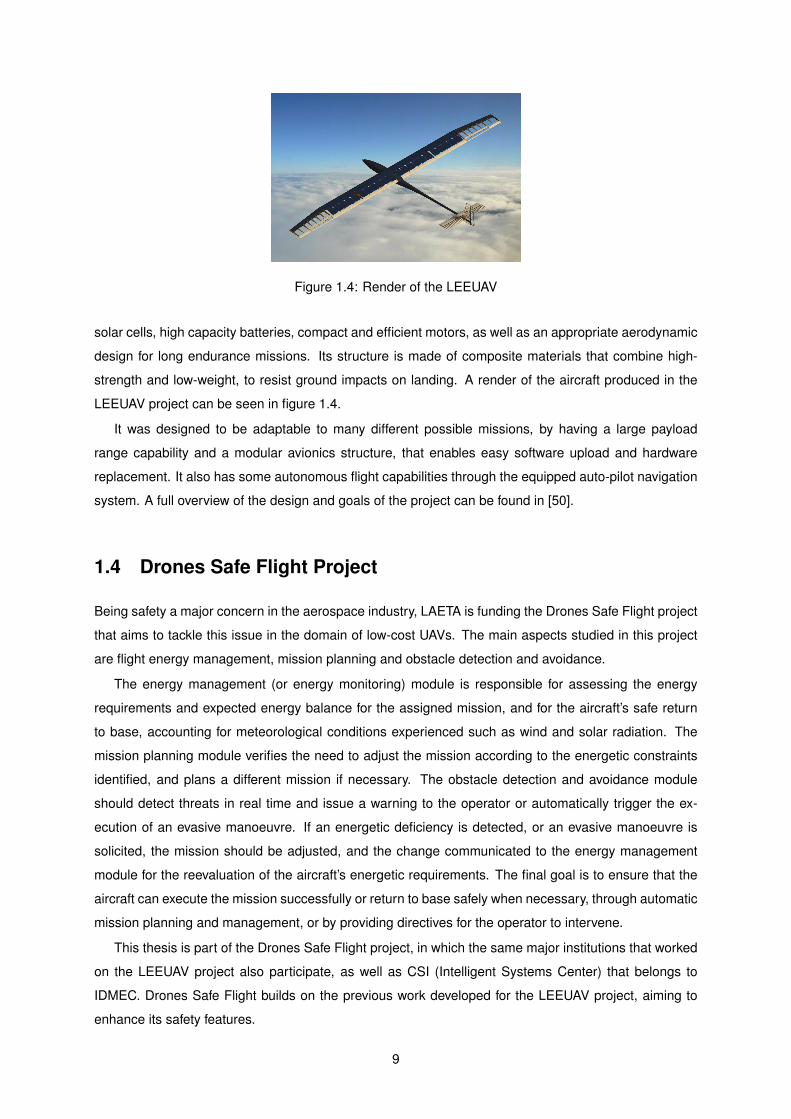
Figure 1.4: Render of the LEEUAV
solar cells, high capacity batteries, compact and efficient motors, as well as an appropriate aerodynamic
design for long endurance missions. Its structure is made of composite materials that combine high-
strength and low-weight, to resist ground impacts on landing. A render of the aircraft produced in the
LEEUAV project can be seen in figure 1.4.
It was designed to be adaptable to many different possible missions, by having a large payload
range capability and a modular avionics structure, that enables easy software upload and hardware
replacement. It also has some autonomous flight capabilities through the equipped auto-pilot navigation
system. A full overview of the design and goals of the project can be found in [50].
1.4 Drones Safe Flight Project
Being safety a major concern in the aerospace industry, LAETA is funding the Drones Safe Flight project
that aims to tackle this issue in the domain of low-cost UAVs. The main aspects studied in this project
are flight energy management, mission planning and obstacle detection and avoidance.
The energy management (or energy monitoring) module is responsible for assessing the energy
requirements and expected energy balance for the assigned mission, and for the aircraft’s safe return
to base, accounting for meteorological conditions experienced such as wind and solar radiation. The
mission planning module verifies the need to adjust the mission according to the energetic constraints
identified, and plans a different mission if necessary. The obstacle detection and avoidance module
should detect threats in real time and issue a warning to the operator or automatically trigger the ex-
ecution of an evasive manoeuvre. If an energetic deficiency is detected, or an evasive manoeuvre is
solicited, the mission should be adjusted, and the change communicated to the energy management
module for the reevaluation of the aircraft’s energetic requirements. The final goal is to ensure that the
aircraft can execute the mission successfully or return to base safely when necessary, through automatic
mission planning and management, or by providing directives for the operator to intervene.
This thesis is part of the Drones Safe Flight project, in which the same major institutions that worked
on the LEEUAV project also participate, as well as CSI (Intelligent Systems Center) that belongs to
IDMEC. Drones Safe Flight builds on the previous work developed for the LEEUAV project, aiming to
enhance its safety features.
9

1.5 Objectives and Achievements
The overall goal of this thesis is to contribute to the increase in low-cost UAV safety, through the devel-
opment of a system capable of generating an updated estimate of the state of total energy remaining
onboard the aircraft at the end of the mission (the margin remaining in terms of energy), capable of
being run on the airborne avionics hardware. This is accomplished by constantly monitoring the avail-
able energy onboard, the aircraft’s energy consumption, the expected required energy to complete the
mission and the solar energy available. The first estimation is done pre-mission (offline) and later the
update of the estimate is periodic as the mission progresses (online), taking into account the conditions
experienced (wind, solar radiation, handicapped airframe or trajectory change, either due to a pilot or
ground control command or automatic obstacle avoidance manoeuvres), as well as those predicted for
the remainder of the mission.
This system is expected to be able to, in the future, interact with other modules studied and developed
in other theses on the topics of mission planning and obstacle detection and avoidance, that are also
part of the Drones Safe Flight project, enabling better energy awareness when planning a mission or
advising a mission adjustment or a return to base if the energy margin drops below a defined safe value.
Despite its association with the LEEUAV project developed previously, this work aims to be general
enough to be adaptable to other aerial vehicles, both fixed wing and multirotor platforms.
With this in mind, the following tasks are expected to be accomplished:
• Model the energy available from all sources
• Model the solar energy harvesting methods
• Model the mission energy requirements
• Model the energy balance for the mission
• Identify the equipment necessary to perform the necessary parameter measurements
• Perform case study simulations to assess the energy monitoring module’s performance
• Demonstrate the viability of the proposed models for the energy monitoring module
Development of a system with the capacity to generate an updated estimate of the state of the total
energy remaining onboard an aircraft at the end of the mission is, to the best knowledge of the author,
scarcely discussed in the literature. The closest example found relating to the energetic evaluation of
a given mission is presented in reference [4]. In that work the energy assessment is used to perform
offline mission feasibility tests, complemented by an online fail-safe feature in which the UAV returns to
the launch position in case of insufficient energy to complete the mission. This is very similar to the
goal of the EMS required for the Drones Safe Flight project, although in [4] the environmental conditions
are not accounted for in these estimates, which should influence the return to launch feature developed,
since it is assumed that this command is triggered when the required energy to return to the launch
position (without accounting for wind) is equal to the remaining available energy in the batteries, which
in reality could potentially lead to insufficient energy to complete the return to launch command. For the
Drones Safe Flight project, it is also not required that, in case of an energy deficiency, the UAV returns
to the initial position. The energy monitoring module is simply required to communicate the situation to
10

the mission planning module in order for the mission to be adjusted (which may or may not involve a
return to the launch position).
In [21] the energy margins of a perpetual endurance mission are predicted, although in this work
the required energy to complete the mission is assumed constant throughout the whole flight. The
estimates are also not updated given the experienced flight conditions, since this work only intended to
demonstrate the perpetual endurance capacity of the aircraft considered.
As such, this thesis contributes to the reinforcement of the literature regarding energy balance and
energy awareness estimates for UAVs, introducing methods not previously considered to periodically
evaluate the capacity of a given aircraft to complete the assigned mission, in real time, and considering
the influence of wind.
1.6 Thesis Outline
The remainder of this thesis is organized as follows:
Chapter 2 describes how the energy flows in the aircraft system and breaks down the problem of
energy estimation, starting with a description of the main forces acting on the aircraft and how they
relate to the required power, then the main types of energy sources used onboard UAVs are described
as well as their basic physical principles of operation and it ends with a discussion of some energy
management strategies described in the literature.
Chapter 3 introduces the mathematical models used to represent each term of the energy estimation
problem, divided in past energy balance, related to online obtained sensor measurements, and future
estimated energy balance, in which the problem of estimating the required energy to finish the mission
as well as a solar energy harvesting model proposed in the literature are explored.
Chapter 4 relates to the integration of the EMS on an aircraft. It describes the physical quantities
that have to be measured in order for the proposed system to output the desired estimates and the
corresponding required instrumentation is discussed, with some hardware being recommended for the
particular implementation of the Drones Safe Flight project.
In chapter 5 a Simulink R© model of a multirotor is used to demonstrate the procedure of calibrating
a correction factor (further discussed in section 3.2.1) and presents a qualitative discussion of the con-
sequences of using the obtained correction factor on the performance of the EMS, which is qualitatively
validated.
Chapter 6 also aims to qualitatively validate the proposed EMS, however the simulations performed in
this chapter present different methods to calculate the required energy to complete the mission relative
to chapter 5. The simulations are performed for the case of the LEEUAV, for which a Simulink R© model
was not available, thus only offline pre-flight energy balance estimates were obtained.
Finally, chapter 7 presents the conclusions of this work as well as future work to be developed.
11

12

Chapter 2
Energy Flow in UAVs
Estimating the energy remaining in the energy sources of an UAV at the end of a given planned mission,
and updating this estimate as the mission progresses, is the main focus of this thesis. The contents of
the following two chapters will establish the foundations and mathematical models used to arrive at this
estimate, both in the offline pre-mission simulation and online.
Figure 2.1: Energy balance at end of mission
An overview of the process is represented in figure 2.1. In essence, for a given instant during the
mission, this is an energy balance problem. In order to solve it, it is necessary to study the flow of
energy into and out of the system. The system in study is the group of energy sources available to
the aircraft. The problem of energy balance is divided in two stages. This is due to the fact that in
general, the balance of energy is calculated in the middle of the mission (at generic present instant
t), and exclusively looking at the past energy flow only allows the computation of the present state of
the system, which is insufficient to decide whether or not the system has enough energy to complete
the planned mission, and therefore the future energy flow has to be predicted in order to arrive at the
estimated final state of the system. Since naturally there will be a discrepancy between the expected
future consumption, predicted at a previous instant, and the amount of energy that will actually be spent
in the future, the estimate for the final state of the system has to be periodically updated, therefore the
13

balance of energy is constantly being recalculated for the full duration of the mission.
First the past energy flow is analysed, starting with the initial state of the system, the energy available
in all energy sources at the start of the mission Esources,t0 (modelled in section 3.1.1). Then it is neces-
sary to subtract the energy that has flown out of the system, the energy that has been measured to be
consumed since the start of the mission until the present moment Econs,t0→t (modelled in section 3.1.2),
and add the energy that has flown into the system, the measured harvested solar energy, from the start
until the present moment Esolar|harv,t0→t (modelled in section 3.1.3). This results in the present state of
the system, the energy available in the energy sources in the present (at time instant t) Esources,t, with
the corresponding mathematical description being given by
Esources,t(t) = Esources,t0 + Esolar|harv,t0→t(t)− Econs,t0→t(t) . (2.1)
Afterwards, the future energy flow is estimated. Knowing the present state of the system all that is
left to do is subtract the expected energy to flow out of the system in the future, the estimated required
energy to complete the mission Ereq,t→tf (modelled in section 3.2.1), and add the expected energy to
flow into the system in the future, the solar energy expected to be harvested in the remainder of the
mission Esolar|pred,t→tf (modelled in section 3.2.2). This in turn results in the estimated final state of the
system, the estimated remaining energy in the sources at the end of the mission Erem,tf , mathematically
described by
Erem,tf (t) = Esources,t(t) + Esolar|pred,t→tf (t)− Ereq,t→tf (t) . (2.2)
Notice that all these quantities are a function of mission time, except for the energy available in the
sources before the flight, since that is a constant amount.
This chapter presents some theoretical background related to the energy flow in UAVs and the energy
balance problem that is being studied. It is divided in three sections that cover energy consumption,
energy storage and energy management. The first section starts by generally discussing the energy
requirements of aircraft and how energy is consumed, defining the forces that apply to all flying vehicles
and their relationship to power required. In the second section, the most commonly types of energy
sources used in UAVs in the present are introduced, as well as the basic physical principles that describe
their operation. The third section closes the chapter with a discussion of possible energy management
procedures that can be implemented in UAVs in order to optimize energetic efficiency.
2.1 Energy Requirements
According to Newton’s second law, the net force ~F acting on an object is proportional to the rate of
change of linear momentum with time, which translates to (2.3) when the mass m of the object is con-
stant,~F = m
d~v
dt= m~a . (2.3)
Indeed this is the case when dealing with electric propulsion vehicles, such as most UAVs. Hybrid
14

propulsion aircraft have variable mass due to the consumption of fossil fuels or fuel used in fuel cells, in
which case the more general statement of Newton’s second law (net force acting on an object equals
time change of linear momentum of the object) has to be used.
The work w done by a force ~F on an object, is given by
w =
∫~F · d~s , (2.4)
where d~s is the infinitesimal displacement vector.
Power P is defined as the time derivative of work, or more generally of energy E. Another possible
definition of power is the dot product between a force acting on an object and the velocity ~v of the object,
P =dE
dt= ~F · ~v . (2.5)
The energy required by an aircraft to fly is directly related to the forces it has to overcome to do so,
namely its weight and aerodynamic drag. To overcome weight the aircraft has to produce lift, and to
overcome drag the aircraft has to produce thrust (although gliders are an exception since they do not
produce thrust, multirotors only produce thrust, not lift, and balloons do not produce thrust, only lift). Lift
is mostly produced by the wings as a consequence of airflow around them, and therefore lift generation
does not directly require energy consumption. An aircraft’s propulsion system, on the other hand, is
responsible for generating thrust, resulting in forward motion, and as thrust and velocity increase, so
does the velocity of airflow around the wings and therefore lift. As such, this is the system that is
responsible for most of the aircraft’s energy consumption. Other actuators (usually electrical servos)
that enable manoeuvring also consume some energy, as well as onboard avionics, such as sensors,
communication equipment and processors.
Figure 2.2: Force diagram during a generic flight stage
In figure 2.2, T is the thrust, D is the drag, L is lift, W is the weight of the aircraft, γ is the climb
angle, θ is the pitch angle, α is the geometric angle of attack and αT is the thrust angle (which is
assumed positive in the anti-clockwise direction, however in this work it will be assumed to equal zero).
15

The pitch angle is related to the geometric angle of attack and climb angle according to
θ = γ + α . (2.6)
The geometric angle of attack is related to the absolute angle of attack αabs by
αabs = α− αL=0 , (2.7)
where αL=0 is the angle of attack at zero lift.
The weight of a constant mass aircraft is given by
W = mg , (2.8)
where g is the acceleration of gravity on Earth. When the mass changes with time, the weight of the
aircraft will of course be a function of time.
For an aircraft to take-off and remain in flight it has to produce enough lift to overcome or balance its
weight respectively. Lift is defined by
L =1
2ρv2SCL = qSCL , (2.9)
where ρ is the air density, v is the TAS, S is the wing surface area, CL is the lift coefficient and q is the
dynamic pressure, defined as
q =1
2ρv2 . (2.10)
The air density varies with altitude, temperature, pressure and humidity, and the lift coefficient is a
function mainly of the aircraft shape, angle of attack, Reynolds number and Mach number.
The drag affecting the aircraft is defined similarly to the lift,
D =1
2ρv2SCD = qSCD . (2.11)
The only difference is that in the case of drag, instead of the lift coefficient CL, the drag coefficient CD
appears in the equation. Both of these coefficients can be obtained through wind tunnel tests, numerical
simulations or using well documented empirical relationships expressed in graphs and tables.
To overcome drag the aircraft produces thrust in order to increase its velocity and produce forward
motion. The thrust generated depends on the propulsion method and its specifications, as well as the
applied throttle.
To evaluate the net force acting on the aircraft during different flight stages, a generic bidimensional
mission profile, represented in figure 2.3 is used.
According to the reference frame in the force diagram of figure 2.2 it follows from (2.3) for the longi-
tudinal motion,
16

Figure 2.3: Generic mission profile
∑Fx = max ⇔ Tcos(θ)−Dcos(γ)− Lsin(γ) = max∑Fz = maz ⇔ Tsin(θ)−Dsin(γ) + Lcos(γ)−W = maz
(2.12)
Here the mass of the aircraft is assumed to be constant, and ax and az are the horizontal and vertical
resulting accelerations respectively. Depending on the flight stage, the values of the forces, angles and
accelerations will vary.
• Take-off and Landing
In both take-off and landing there is no vertical resulting acceleration. Since the aircraft’s landing
gear is touching the ground, there is an additional vertical normal force term that, summed to lift and
weight, will net zero vertical force. During these stages the horizontal acceleration is not null because
the aircraft is still increasing its speed to generate enough lift for take-off, or decreasing its speed in case
of landing. These conditions are expressed as
γ = 0
az = 0
ax > 0 (during take-off)
ax < 0 (during landing)
(2.13)
• Climb and Descent
The only difference between climb and descent is the sign of the climb angle. In steady conditions
yields ax = 0 ∧ az = 0 (constant speed)
γ > 0 (during climb)
γ < 0 (during descent)
(2.14)
• Cruise
During cruise the flight is horizontal and it may or may not be accelerated in the horizontal axis. The
17

cruise conditions are described by
γ = 0
ax = 0 ∧ az = 0 (level flight at constant speed)
ax 6= 0 ∧ az = 0 (accelerating level flight)
(2.15)
If the total drag curve of the aircraft is known for every airspeed, the power required curve can be
obtained by assuming that thrust equals drag (for non-accelerated level cruise only), and multiplying
drag by the airspeed. This relationship is expressed as
P = Dv =1
2ρv3SCD . (2.16)
The black bold curve in figure 2.4 represents a typical required power curve to fly at a given airspeed,
for a propeller aircraft and assuming a constant high-lift device configuration. At airspeeds below or
above the minimum power required one, the power required increases due to an increase in induced drag
(with pressure drag contributing slightly as well) and due to an increase in parasitic drag respectively.
Figure 2.4: Power available vs power required (source: www.recreationalflying.com)
It is important to note however that for propeller aircraft the maximum power available varies with
altitude (due to decreased air density with altitude), and when full throttle is applied at altitudes above
sea-level, the maximum power available will drop to a percentage of the rated power, except for aircraft
with electric motors in which case only the propeller efficiency depends on air density.
In the case of multirotors, the force diagram considered is slightly different, and shown in figure 2.5.
Multirotor aircraft can adjust the direction of thrust by having different speeds on the propellers at a
given time, and will be affected by drag in the opposite direction of their motion. Naturally the weight
of the aircraft is the last force represented in the diagram. Equation (2.17) follows from the previous
diagram.
18

Figure 2.5: Force diagram for a generic multirotor aircraft
∑Fx = max ⇐⇒ Tsin(σ)−Dcos(γ) = max∑Fz = maz ⇐⇒ Tcos(σ)−Dsin(γ)−W = maz
(2.17)
Comparing equations (2.12) and (2.17) it can be seen that the fixed wing and the multirotor cases
can be generalized to the same set of governing equations by defining L = 0 and θ = 90o − σ in the
former case.
2.2 Energy Sources
Energy sources supply the energy the aircraft and its systems require to function properly. The following
sections represent the main sources of energy found in most UAVs, such as fossil fuels, batteries, fuel
cells and solar energy harvesting. Their basic physical principles of operation are briefly described as
well as the various technologies existing today.
2.2.1 Fossil Fuels
Fossil fuels (coal, petroleum and natural gas) are non renewable energy sources based on mineral
hydrocarbon compounds. Today, they supply approximately 85% of the world’s energetic needs, and
are mainly used for transportation and electricity generation [51]. The main uses for petroleum are the
production of fuels for combustion engines used in vehicles, such as gasoline, diesel and jet fuel [51].
In the aviation industry the fuel market comprises jet fuel, which can be kerosene-type or naphtha-
type (also known as wide-cut fuel), and aviation gasoline (Avgas). In commercial aviation Jet A and Jet
A-1, kerosene-type jet fuels, dominate the market. The main difference between the two are the lower
freezing temperature of Jet A-1, making it ideal for intercontinental flight. The military mostly uses JP-8,
which is similar to Jet A-1, but contains more additives to protect against corrosion and static, however
it has recently started shifting to commercial jet fuel. Less used than kerosene-types are the Jet B
and JP-4 naphtha-type jet fuels. There is also aviation gasoline, consumed mostly by smaller aircraft,
19

Table 2.1: Aviation fuels specific energy
Fuel Type Fuel Specific energy (MJ/kg)Naptha-type fuels Jet B 43.54Kerosene-type fuels Jet A 43.28Aviation Gasoline Avgas 43.71
Table 2.2: Battery types and respective properties (adapted from [55] and [56])
TypeVoltage(V)
Energy Density(Wh/liter)
Specific Energy(Wh/kg)
Lifetime(cycles)
Lead-acid 2.1 70 30 300NiMH 1.4 240 75 800LiCoO2 3.7 400 150 1000LiMn2O4 4.0 265 120 1000LiFePO4 3.3 220 100 3000Li-polymer (used in UAVs) - - 145-240 -Li-S (used in UAVs) - - 350 -
however its market share is very small, only around 1% of the total aviation fuel market [52], [53]. Table
2.1 establishes a comparison between the specific energies of various aviation fuels according to a
technical review by Chevron [54].
2.2.2 Batteries
Batteries are a very common energy source whose applications span a variety of portable electronic de-
vices. Rechargeable batteries are especially interesting because they can be reused many times. The
most common types of rechargeable batteries are based on lithium or lead, but the general working prin-
ciple is the same. During discharge the anode (the negative electrode during discharge) is oxidized and
electrons flow from it, through an electric circuit, to the cathode (the positive electrode during discharge),
which is reduced, while the ions formed during the chemical reactions happening in the electrodes are
transported through an electrolyte between them. The flow of electrons through an external circuit is
what allows the battery to power a load [55]. Table 2.2 summarizes the properties of common battery
types.
According to [56], for solar powered UAVs, the less energy dense battery technologies, such as alka-
line, lead-acid, nickel cadmium (NiCd) and nickel metal hydride (NiMH), are not used, since a significant
portion of the total weight of the aircraft is due to the batteries onboard. Lithium-ion, lithium-ion polymer
and lithium sulphur are the best alternatives to power solar powered aircraft due to their higher energy
densities. Lithium-ion polymer batteries have the same properties of their lithium-ion counterparts, but
are lighter and can be shaped in any form. In the present, lithium-sulphur (Li-S) batteries have the high-
est theoretical specific energy of 2600 Wh/kg, which is a significant increase over common lithium-ion
and lithium-ion polymer batteries used in solar powered aircraft, which have around 145-240 Wh/kg,
however the Zhephyr 7 solar powered high-altitude long endurance (HALE) UAV only demonstrated that
20

Table 2.3: Fuel cell specific energy for a given power range
Fuel Cell Power Range Specific Energy (Wh/kg)<2W Micro Portable 11010-50W Small Portable 150100-250W Medium Portable 250
its lithium-sulphur battery could achieve 350 Wh/kg in 2010 [56].
2.2.3 Fuel Cells
Fuel cells (FCs) produce an electrical current by promoting chemical reactions involving oxygen and
hydrogen. The exact reactions happening at the electrodes, as well as the electrolyte used vary de-
pending on the type of FC. In the simplest case, an acid electrolyte is used, the hydrogen gas ionizes
in the anode, releasing electrons and energy. In the cathode, the oxygen reacts with electrons from the
electrode and the H+ ions from the electrolyte, forming water [57].
Usually the voltage of a single FC is rather small when drawing current, and for this reason they are
often connected in series to produce higher voltages. FCs that are connected in this manner are refered
to as a stack. Some issues that compromise the effectiveness of FCs are the slow reaction rates (which
leads to low current and power) and the fact that hydrogen in not easily available as a fuel. Also they are
currently expensive, but their main advantages are greater efficiency compared to combustion engines,
their simplicity, low emissions and silent operation [57].
References [58] and [59] highlight some applications for different types of FC. Proton exchange
membrane fuel cells (PEMFC) are very versatile and are promising candidates for transport applica-
tions, including UAVs, due to their high power density, fast start-up time, high efficiency, low operating
temperature and easy and safe handling. Alkaline FCs have a great performance when operating with
pure hydrogen and oxygen, but since they are very sensitive to impurities they are mostly used for ex-
traterrestrial applications. Phosphoric acid fuel cells (PAFC), solid oxide fuel cells (SOFC) and molten
carbonate fuel cells (MCFC) are indicated for static applications, namely for energy production, although
some research is being conducted on using SOFC in UAVs, such as [60] and [61]. Reference [58] also
indicates an average specific energy for FCs within a given power output range, which are summarized
in table 2.3.
2.2.4 Solar Energy
The Sun is an incredibly powerful source of energy. The average power density reaching the Earth,
just outside its atmosphere is 1366 W/m2, which means that each year the equivalent of 5.46 × 1024 J
reaches the Earth as solar radiation.
Solar cells make use of the photoelectric effect to convert solar radiation into electric current (if the
circuit is closed), that can be used to power a load. Most solar cells are made of semiconductors
with photoemissive properties. When light with sufficient energy hits the surface of the semiconductor,
21

electrons are expelled from the bonds between the semiconductor atoms, leaving behind a hole (a
deficiency of electrons) [62].
Figure 2.6: Operation mechanism of a solar cell (source: www.solarproductsstore.com)
By introducing impurities in the semiconductor (in a process known as doping), the semiconductor
is left with a layer with excess electrons, the n-type side, and a layer with excess holes, the p-type side.
When both layers are put into contact, the free electrons from the n-type side rush to fill the holes in
the p-type side, and vice-versa, such that at the interface the n-type side becomes positively charged,
and the p-type side becomes negatively charged, resulting in an electric field (or a potential barrier) that
makes it increasingly difficult for additional electrons to cross it to the p-type side, and for additional
holes to cross it to the n-type side.
The charges are thus separated by this mechanism. If for example, light with sufficient energy creates
an electron-hole pair in the n-type side of the cell, the hole is accelerated by the electric field to the n-
type side, while the electron is repelled by it, remaining in the n-type side. If the n-type side is connected
to the p-type side through an external circuit, it can perform useful work on a load, before the electrons
have a chance to recombine with the holes in the p-type side [62]. Figure 2.6 illustrates the operation of
a solar cell.
The main factors affecting the amount of energy collected by a PV panel are the efficiency of the
solar cells, the area of the PV panel, the geographic location (mostly latitude), the solar zenith angle
(defined as the angle between the direction of the center of the sun and the local zenith), which varies
with day of the year and hour of the day, the orientation of the solar panel (affecting the incidence angle
of the solar rays on the PV panel), the weather and temperature. Shade and dirt can also hinder the
power output of the solar panel, since the solar cells are usually connected in series, and if one cell is
dirty or in the shade, the whole panel output is compromised [62].
Crystalline silicon solar cells dominate the market, having around 90% share [63], with efficiencies
ranging between 20-24.7% [55]. There are two types of crystalline silicone solar cells, mono crystalline,
the most efficient and expensive (although efficiency lowers with higher temperatures), and polycrys-
talline, less efficient and less expensive than their mono crystalline counterparts (but also less sensitive
22

Figure 2.7: Photovoltaic cell efficiencies (source: National Renewable Energy Laboratory (NREL))
to temperature changes). However in the present, the efficiency and cost of the last is rivalled by
the technological development of the most efficient thin-film solar cells, copper indium gallium selenide
(CIGS) (efficiency can be as high as 19.9% [55]) and cadmium telluride (CdTe) (best efficiency of around
16.5% [55]), that may even be better suited in hotter climates, due to better temperature tolerance [63].
Nonetheless, low-cost manufacturing and rising efficiencies of crystalline silicone solar cells are decreas-
ing the confidence in the thin-film market [63]. The cheapest and less efficient (best experimental cell
efficiency of 10% [55]) thin-film solar cell is amorphous silicon, although their market share is less than
1%, declining in favour of the other more efficient alternatives that keep getting cheaper as technology
and production methods progress [63] (another source for price comparison between solar cell types:
http://www.greenmatch.co.uk/solar-energy/solar-cells/types-of-solar-cells). Organic solar
cells are an emerging PV technology, however their efficiency is still relatively low. Although different
sources disagree on the exact values of efficiency for each solar cell technology, the estimates are rel-
atively close and the order from highest to lowest efficiency is maintained. Figure 2.7 highlights the
evolution of the efficiencies of PV cells until the present.
2.3 Energy Management
Energy management methods aim to make the most efficient use of available energy. In conjunction
with efficient mission planning algorithms, this results in minimum energy consumption and extended
endurance, which is important in battery powered UAVs, especially multirotors, that tend to discharge
their batteries relatively fast.
In an aircraft that only possesses one type of energy source all the energy required to fly and operate
23

the vehicle will come from that source. However it is common to have a hybrid setup installed in an UAV,
including more than one energy source. The most common one is the electric propulsion vehicle, that
carries a rechargeable battery (or batteries) and recharges them using PV cells. To prevent overcharging
and to increase battery life, many solar powered aircraft incorporate a charge controller (or charge
regulator) connected to their batteries, which manages the current flow to and from them, and may even
protect them against overvoltage. Alternatively, energy harvested through the PV panels can be directly
used to power the aircraft, being supplemented by the battery when necessary.
PV modules have a non-linear current-voltage (I-V) characteristic, and there is only one point at
which it can provide maximum power. However this point changes with load resistance, insulation (solar
radiation intensity) and temperature, and if this factor is not accounted for, the mismatches in impedance
between the PV modules and the load lead to power losses. The maximum power point tracker (MPPT)
controller tracks the point of maximum power and adjusts the impedance of both the PV modules and
the load, in order to have the maximum amount of power transferred to the load [64]. This particular
setup is illustrated in figure 2.8.
Figure 2.8: Energy management for electric propulsion UAVs
Some research effort [20] is being directed at attempting to have solar powered HALE aircraft re-
main in flight during long periods of time (several days or more), with the goal of eventually substituting
satellites, or complement them for communications, surveillance, telecomunications relay, remote sens-
ing, observation and military purposes, at a lower cost. In order to accomplish this goal an appropriate
energy management system has to be developed. A possible approach, described in reference [20],
suggests a three stage flight.
Stage one happens when enough solar energy is available to be harvested by PV panels and power
the aircraft by itself, and the excess energy collected is used to charge the batteries. Moreover, during
stage one, the aircraft gains as much altitude as possible, storing energy as gravitational potential en-
ergy. During stage two, when the solar power available is not enough to alone power the aircraft and
maintain level flight, the aircraft trades the accumulated potential energy for kinetic energy, remaining in
gliding flight and losing altitude. Finally, stage three starts when the aircraft descended into the lowest
operational altitude, at which point the batteries supply the energy required to maintain level flight, until
enough solar energy is available to restart from stage one, or until the batteries are discharged. The
decision algorithm to perform a 24 hour flight for solar powered UAVs is illustrated in figure 2.9.
24

Figure 2.9: Energy management strategy for a 24 hour flight for solar powered aircraft
When a combination of fossil fuels and rechargeable batteries, or fuel cells and rechargeable batter-
ies are used, it would be wise to use the energy from the batteries when possible and avoid consuming
energy from the non rechargeable sources, since the energy consumed from the batteries could be
recovered by means of solar energy harvesting through PV cells. Since batteries are usually heavy, in
most cases they end up being a secondary onboard power source, while FCs or fossil fuels power the
aircraft during the most power demanding manoeuvres.
Reference [22] studies an energy and power management system (PMS), with a FC and battery
combination. The PMS optimizes the amount of energy used by the FC and controls the direction of the
power flow of the battery depending on the power required by the load and the battery SoC, by regulating
the airflow and air pressure reaching the FC system.
Three modes of operation are described: during start-up, the battery powers the propulsion system
while the FC system gradually starts its operation (slowly increasing the power provided to the load), and
once the FC is fully operational, the battery is recharged to at least 90% of its capacity before take-off;
during the most power demanding conditions (take-off, climb and maximum velocity) both the battery
25

and and the FC power the propulsion system; when the aircraft is in cruise, only the FC supplies power
to it, while also recharging the battery.
In reference [65] a three power source architecture, consisting of PV cells, a FC and a battery, is
studied, in passive and active configurations. In the passive configuration the output voltages of all
sources are matched to the power bus voltage, and no converters or controllers are used. In the active
configuration the PV cells have a MPPT controller connecting them to the bus, while the FC has DC/DC
converters, and the battery has a charge/discharge controller. The PV cells and FC operate as the
main power sources, having the battery supplement them in the most power demanding manoeuvres
(take-off and transient flight). The active PMS is able to maintain the battery SoC above a minimum
value, improving system safety and guaranteeing a more efficient power distribution. However passive
PMS have some advantages, namely the simpler hardware, which also avoids power losses in the
conversions, and weight reduction. For this reason passive PMS are more widespread in smaller UAVs.
26

Chapter 3
Energy Estimation Models
This chapter presents the mathematical models used to estimate each of the components of equations
(2.1) and (2.2). The first section relates to the description of the past energy flow (based on sensor
measurements from t0 to instant of calculation t), including the initial energy contained in the energy
sources (the initial state of the system), the energy consumed until t and the solar energy harvested
until t. Afterwards, in the second section, the future energy flow predictions are introduced, including the
expected required energy to complete the mission, and the amount of energy expected to be harvested
through the solar panels in the remainder of the mission.
3.1 Past Measured Energy Flow
Assessing the energy available in the sources of the aircraft at a given time instant (Esources,t) requires
measurements of current I and voltage U in different positions of the electric circuits onboard, illustrated
in figure 3.1, as well as of volumetric fuel flow rates Vfuel in case the aircraft is powered by fossil
fuels, as illustrated in figure 3.2, such that the past flow of energy into and out of the system can be
evaluated. Mechanical energy must also be considered, since it varies during the mission, increasing
when propulsion energy is traded for it, and decreasing when velocity or altitude decrease. FCs will not
be considered in this thesis due to the low percentage of UAVs that rely on this energy source in the
present.
An alternative way to express Esources,t, aside from the one in (2.1), is given by
Esources,t(t) = Ebattery,t(t) + Efuel,t(t) + Ep(t) + Ek(t) , (3.1)
where Ebattery,t and Efuel,t are the energy available in the battery and in the fossil fuel tank at time
instant t, respectively, and Ep and Ek are the potential (measured relative to the altitude of the landing
point) and kinetic energies available to the aircraft, respectively.
Assuming that the energy available in the battery is proportional to its capacity and voltage, the
voltage is constant throughout the discharge and the capacity of the battery decreases linearly with
27

Figure 3.1: Possible points of voltage and current measurement (in blue) in the electric circuits of theaircraft
Figure 3.2: Point of fuel volumetric flow measurement (in blue) in the aircraft
discharge, the energy available in the battery at time instant t is given by
Ebattery,t(t) = Ebattery,t0 −∫ t
t0
Ebattery(t)dt , (3.2)
where Ebattery,t0 is the energy available in the battery at the beginning of the mission (initial state of the
battery) and Ebattery(t) is the instantaneous power flow of the battery, which can be either positive or
negative, depending on whether more energy is consumed than the amount that is harvested or if more
energy is harvested than the amount that is consumed, respectively. As such, the term∫ t
t0Ebattery(t)dt
represents the energy change in the battery until t.
The energy available in the fuel tank at time instant t is given by
Efuel,t(t) = Efuel,t0 −∫ t
t0
Efuel(t)dt , (3.3)
where Efuel,t0 is the energy available in the fuel tank at the beginning of the mission (initial state of
the fuel tank) and Efuel(t) is the instantaneous power consumption equivalent to the time change in the
amount of energy contained in the fuel mass leaving the tank. Thus,∫ t
t0Efuel(t)dt represents the energy
consumed from the fuel tank (equivalent to the energetic content of the mass of fuel consumed) until t.
The potential energy available at time instant t is simply obtained by measuring the altitude of the
aircraft ht in the same instant, and calculating it through its definition
Ep(t) = mg(ht(t)− htf ) . (3.4)
where htf is the altitude of the landing point. Notice that Ep will have a negative value whenever the
28

aircraft is at an altitude below that of the landing point, meaning that (the symmetric of) this amount of
energy has to be consumed by the propulsion system in order to finish the mission with a larger potential
energy than the one at time instant t.
When calculating the kinetic energy at a given instant, it is necessary to consider the influence of the
wind. Therefore the ground speed is required to compute its value. The diagram of figure 3.3 illustrates
the relationship between the relative wind (−→vA), the wind speed (−→vw) and the ground speed (−→vG).
Figure 3.3: Relationship between relative wind, wind velocity and ground speed
Therefore it follows that−→vG = −→vA +−→vw . (3.5)
The kinetic energy of the aircraft at time instant t is then obtained by measuring its ground speed in
the same instant, and calculating it through its definition
Ek(t) =1
2mv2G(t) . (3.6)
Another possible source of mechanical energy is dynamic soaring [13], which consists in harvesting
energy from an environment where wind gradients are present, but the complexity introduced by this
technique goes beyond the scope of this thesis.
In the following three sections the new terms introduced, as well as those from chapter 2 related to
past measurements, are discussed.
3.1.1 Initial Energy Stored in the Sources
The energy available in the energy sources at the start of mission is modelled by
Esources,t0 = Ebattery,t0 + Efuel,t0 + Ep,t0 + Ek,t0 , (3.7)
where Ebattery,t0 and Efuel,t0 are the energy available in the battery and in the fossil fuel tank at the start
of the mission respectively, and Ep,t0 and Ek,t0 are the potential and kinetic energies of the aircraft at
the start of the mission, respectively. The initial energy stored in the battery is given by
Ebattery,t0 = SoCQnomUnom3600 , (3.8)
where SoC is the state of charge of the battery (between 0 and 100%), Qnom is the nominal charge of
the battery and Unom is the nominal voltage of the battery. This model assumes that the battery is not
29

affected by Peukert’s law [26], and that the SoC is known from the pre-flight charging process.
The initial energy contained in the fuel tank is related to the volume of fuel it contains, expressed in
(3.9).
Efuel,t0 = ufuelmfuel,t0 = ufuelρfuelVfuel,t0 , (3.9)
where ufuel is the specific energy of the fossil fuel, ρfuel is its density and Vfuel,t0 is its volume at
the beginning of the mission. This assumes ρfuel is estimated for a given temperature and Vfuel,t0 is
measured.
The initial potential energy is
Ep,t0 = mg(ht0 − htf ) , (3.10)
where ht0 is the altitude of the aircraft at the start of the mission.
Finally, the initial kinetic energy of the aircraft is zero, since its ground speed is also zero.
3.1.2 Energy Consumed
The consumed energy Econs,t0→t from the start of the mission until a given time instant t, is given by the
sum of the energy consumed from the battery (given by the sum of the change in energy of the battery∫ t
t0Ebattery(t)dt and the amount of energy harvested through the PV panels Esolar|harv,t0→t(t)), and the
energy consumed from the fuel tank∫ t
t0Efuel(t)dt. The model for the energy consumed is described by
Econs,t0→t(t) =
(∫ t
t0
Ebattery(t)dt+
∫ t
t0
Esolar|harv(t)dt
)+
∫ t
t0
Efuel(t)dt , (3.11)
Taking into account the nomenclatures of figures 3.1 and 3.2, the terms of equation (3.11) are given
by equations (3.12) through (3.14),
∫ t
t0
Ebattery(t)dt =
∫ t
t0
UBIBdt , (3.12)
∫ t
t0
Efuel(t)dt = ufuelρfuel
∫ t
t0
Vfueldt , (3.13)
where Vfuel is the fuel volumetric flow. This assumes that the quantities UB , IB , UPV , IPV and Vfuel are
measured. It is important to notice that IB can be both positive and negative, depending on whether the
battery is being discharged or charged, respectively.
3.1.3 Solar Energy Harvested
By measuring voltage UPV and current IPV from the PV panel according to figure 3.1, and integrating
the product of these quantities over time, it is possible to obtain the solar energy harvested from the
beginning of the mission until time instant t, as
∫ t
t0
Esolar|harv(t)dt =
∫ t
t0
UPV IPV dt . (3.14)
30

3.2 Future Predicted Energy Flow
To estimate the energy remaining in the sources at the end of the mission Eremaining,tf (the final state
of the system), it is necessary to estimate, at a given time instant, how much energy is still required to
finish the mission and how much solar energy is expected to be harvested until the end of the mission, as
previously shown in (2.2). In the following two sections possible approaches to achieve these estimates
are discussed.
3.2.1 Energy Required
The expected required energy to complete the mission represents an estimate of the future energy flow
out of the system. The main contribution to the consumption of energy comes from the propulsion
system. Avionics equipment and low power actuators (that enable the deflections of flaps, ailerons and
rudder for example) also consume some energy, however it will be assumed, that the contribution of
low power actuators to the total consumption is either small compared to the other power consuming
components, or that it is an approximately constant term that is part of the avionics contribution.
As such, in order to estimate how much energy is required to complete the mission, it is necessary
to estimate the future consumption of the propulsion system Eprop,t→tf , the future consumption of all
the avionics equipment Eav,t→tf and also take into account the change in mechanical energy (∆Ep and
∆Ek) between the instant of calculation t and the end of the mission, leading to
Ereq,t→tf (t) = ∆Ep(t) + ∆Ek(t) + Eav,t→tf (t) + Eprop,t→tf (t) . (3.15)
• Change in mechanical energy
The change in kinetic and gravitational potential energy, from time instant t until the end of the
mission, can be obtained from (3.17) and (3.16) respectively, from the previously introduced definitions
for Ep and Ek.
∆Ep = Ep,tf − Ep,t(t) , (3.16)
∆Ek = Ek,tf − Ek,t(t) . (3.17)
Notice that both these changes can be negative, which happens when the final values of potential
and kinetic energies are lower than the ones at time instant t. This leads to a smaller value of required
energy, since some propulsion energy was already spent in the past in order to increase altitude and
ground speed, and it is at this instant stored as potential and kinetic energy, reducing the amount of
required propulsion energy in the future to finish the mission.
• Avionics required energy
31

The simplest approximation for the energy required to operate all avionic systems (which include
sensors, communications equipment, aerodynamic surface actuators and processors) is to assume that
the power required for their operation is constant throughout the mission. In this case, if there is an array
Pinstruments, whose elements are the (constant) power required to operate each instrument onboard the
aircraft, then the energy required to power the avionics systems is estimated as
Eav,t→tf (t) =∑i
∫ tf
t
Pinstruments,idt (3.18)
• Propulsion required energy
To estimate the required propulsion energy to finish the mission successfully three different ap-
proaches were considered. The first approach is indicated when no experimental data is available,
while the second and third should only be used when it is.
• Method 1 - Multiplying a correction factor by the base prediction
For the first case, the propulsion power required to maintain flight in an equilibrium condition is
initially established. For instance, in multirotors this situation corresponds to the hover flight condition,
while in fixed wing aircraft the cruise condition can be considered. Other researchers have used the
same assumption previously to estimate endurance, such as in [29], in which it is assumed that, while
the multirotor platform is flying, thrust equals weight (equivalent to the hover condition). Notice that
the equilibrium condition may not represent the state of minimum power consumption, for example, the
authors of reference [4] studied the power required to fly a multirotor at different speeds, and the hover
condition was not the state of minimum power required.
Integrating the propulsion power required to fly in the equilibrium condition (Pprop,eq) over the ex-
pected remaining mission time nets the propulsion energy required for flight in this state (Eprop,eq,t→tf ),
as described by
Eprop,eq,t→tf (t) =
∫ tf
t
Pprop,eqdt . (3.19)
However, this estimate is not good enough in itself, since the main goal of implementing the EMS is to
improve UAV safety systems, and an equilibrium condition based estimation for the required propulsion
energy will in some cases result in an underestimate, going against this goal. As such, a correction (or
safety) factor Cf has to be multiplied by this propulsion energy required projection, in order to pull the
estimate closer to the real value, expressed as
Eprop,t→tf (t) = CfEprop,eq,t→tf (t) . (3.20)
Ideally, the result of this correction should be at least equal to the real energy consumption of the
aircraft in the remainder of the mission, or slightly overestimate it, to avoid safety hazards. The correction
factor has to be determined experimentally or through flight simulations, and will be unique for each
aircraft. Simulation tools such as Simulink R© are helpful in this part of the project as discussed in chapter
5.
32

• Method 2 - Finding the propulsion energy required by estimating the required thrust for each mis-
sion segment
An alternative approach that was considered for estimating the required propulsion energy to finish
the mission was to estimate the power required to fly each segment of the planned mission, and integrate
the result over time, based on the required thrust for manoeuvring the aircraft. The force diagram
considered is represented in figure 3.4.
Figure 3.4: Force diagram for a generic aircraft
The balance of forces is therefore given by
L−Wcos(γ) +Bcos(γ) + Tsin(α) = 0
Tcos(α)−D −Wsin(γ) +Bsin(γ) = ma
(3.21)
where B represents the buoyancy force.
Finding an approximation for the thrust required can be challenging depending on what information
is available about the aircraft. To solve the balance of forces of equation (3.21) it is necessary to predict
(or provide an approximation for) the angle of attack or pitch angle, which is not a simple task, since this
depends on the direction of the flow of air around the aircraft, which is very unpredictable.
A possible workaround this limitation is to start by experimentally determining the drag polar curve
(CD = f(CL)) and the relationship between lift coefficient and the angle of attack (CL = f(α)) of the
aircraft (both represented in figure 3.5 for the case of the LEEUAV). There are four unknowns in the
balance of forces (T , D, L and α) which can be obtained through the 2 equations from the force diagram
and from the 2 plots of figure 3.5, assuming the desired acceleration for each mission segment. The
weight and buoyancy (in case the aircraft in study is a dirigible balloon) of the aircraft are known.
With this method, to calculate lift and drag, it is necessary to estimate the air density ρ, which varies
with air pressure p and temperature Tp, as stated in equation (3.22), that in turn vary with altitude,
according to the Earth’s atmosphere standard model, expressed in equation (3.23) for the bottom layer
of the atmosphere [67]. For simplicity, the acceleration of gravity was assumed constant with altitude and
altitude is simply the distance between the aircraft and the surface (instead of the geopotential altitude
defined in reference [67]).
33

Figure 3.5: LEEUAV performance curves [66]
ρ =pM
RTp(3.22)
where M = 0.028964420 kg/mol is the molar mass of dry air and R = 8.31432 J/(mol.K) is the ideal gas
constant.
The model for the temperature and air pressure in the troposphere (altitude below 11 km) is given by
Tp = Tp,0 − LTh
p = p0(Tp
Tp,0)( gMRLT
), (3.23)
where LT = 0.0065K/m is the temperature lapse rate of the troposphere (variation of temperature
with altitude, or temperature gradient), h is the altitude, Tp,0 = 288.15K and p0 = 101325Pa are the
temperature and air pressure at sea level respectively, and g is the acceleration of gravity.
The climb angle γ is the last parameter that has to be determined in order to calculate the required
thrust for a given segment. Assuming that during the mission planning stage a set of waypoints are
chosen for the aircraft to follow, it is possible to calculate this angle between two waypoints. Moreover,
each aircraft has a typical velocity to operate at a given flight condition, in order to optimize performance,
which can be used when predicting the required propulsion energy. Alternatively, the prediction can be
adjusted when different values are desired (for example to achieve a faster mission). The maximum
acceleration of the aircraft is typically known, or can easily be tested, however if a different acceleration
value is desired for a given segment, it can be calculated based on the operational requirements of the
mission (velocity change in a given time interval).
Due to the unpredictability of the effects of wind on the attitude of an aircraft, this is not considered
when predicting its future motion. The influence of attitude corrections on the consumption is, in this
case, small compared to the amount of energy consumed during motion performed with constant atti-
34

tude, and therefore is considered to be zero in order to simplify the estimation process. This means that
the thrust required is studied assuming constant attitude motion for each segment of the mission.
Notice that for multirotors, the orientation of the total thrust (as well as that of the thrust generated by
each propeller) is the same as that of the vertical body axis (assuming no blade flapping effects), and to
maintain a given attitude, the thrust required from each propeller Ti must be the same, and is given by
Ti =T
nprops, (3.24)
where nprops is the number of propellers of the multirotor.
The aircraft types studied in this thesis all use propellers to generate thrust. The power that has to be
transfered to the air by the propellers is related to the thrust required for a given manoeuvre. Knowing
the radius rp of the propellers used, the air density ρ, the angular velocity ωi of the propeller and its
power coefficient Cp,i, using momentum theory [68] it is possible to estimate the mechanical power that
the propeller of an helicopter during hover is required to transfer to the air (Ppropeller,i) through
Ppropeller,i = ρω3i πr
5pCp,i . (3.25)
This expression can then be used as an approximation for the required power that has to be trans-
ferred to the air by each of the propellers of an aircraft.
For a given propeller, the values of ωi and Cp,i necessary for a given manoeuvre, can be ob-
tained from experimental characterization of the propeller or from appropriate tables as a function of
thrust required and airspeed. Tables like this can be obtained from manufacturer data, for example at
www.apcprop.com/v/PERFILES_WEB/listDatafiles.asp (in which performance data is based on vortex
theory). The total propeller power required Ppropeller is then obtained by summing the power required
from each of the individual propellers, as expressed in
Ppropeller =
nprops∑i=1
Ppropeller,i . (3.26)
Finally dividing the total propeller power required by the efficiency of the propulsion system ηprop
results in the propulsion power required to be extracted from the system (energy sources) in the future,
as given by
Eprop = Pprop =Ppropeller
ηprop. (3.27)
The overall efficiency of the propulsion system ηprop is dependent on the efficiencies of its compo-
nents (figure 3.6), thus, the efficiencies of the motor ηmotor, gear box ηgb, propeller ηpropeller and ESC
ηESC , as expressed by
ηprop = ηmotorηgbηpropellerηESC . (3.28)
The efficiency of the propulsion system varies with TAS of the aircraft, therefore it tends to be lower
at take-off and landing and larger during cruise. For simplicity a (different) constant efficiency can be
assumed for each flight stage.
35

Figure 3.6: Propulsion system components
The propulsion required energy is therefore obtained by integrating the propulsion required power
that has to be extracted from the system (energy sources) in the future, yielding
Eprop,t→tf (t) =
∫ tf
t
Pprop dt . (3.29)
• Method 3 - Experimentally determining the required electric power as a function of airspeed
One more possibility to determine the required propulsion and avionics power required is to experi-
mentally characterize the energy requirements of an aircraft as a function of airspeed. Figure 3.7 shows
this relationship for the LEEUAV while in cruise condition. The effect of drag is already accounted for
in the experimental curve, and knowing the required ground speed for each mission segment (as well
as a forecast for the direction and velocity of wind), it is possible to obtain the required avionics and
propulsion energy to finish the mission by integrating the corresponding value of required electric power
Pel from the curve over the expected remaining duration of the mission, as described by
Eav,t→tf (t) + Eprop,t→tf (t) =
∫ tf
t
Pel dt . (3.30)
Notice that since this particular experimental characterization is only valid for cruise, this approach
results in an underestimation of the power requirements for take-off and climb. If a more detailed ex-
perimental characterization of the power requirements for different flight stages was available, a better
quality estimate could be obtained.
Figure 3.7: Power required as a function of airspeed for the LEEUAV during cruise (with photovoltaicpanels installed) [69]
36

• Another considered approach
A final approach that was considered was to estimate future energy requirements of the aircraft based
on past consumption during the same mission. However, this method has problems, namely at the start
of the mission, when there is not enough data available to perform the estimation, and for example at the
start of the cruise stage for a fixed wing aircraft, since during climb (past energy consumption) the energy
requirements of the aircraft are much higher than those for the cruise stage, therefore making predictions
based on past consumption would result in a severe overestimation of future energy requirements. For
these reasons this method was not used during the project.
• Remaining mission duration
To evaluate the integrals used to calculate the terms related to the future energy flow (equations
(3.18), (3.19), (3.29), (3.30) and (3.35)), it is necessary to estimate the remaining mission duration. This
estimate can be obtained by using the equations of the linear uniformly accelerated motion (expressed
in their general form in (3.31)) and solving them for ∆t, using the previously introduced assumption that
the aircraft moves in a straight line, ignoring attitude corrections, and knowing the desired ground speed
and acceleration for each remaining mission segment.
s(t) = s0 + vs,0∆t+1
2a∆t2 , (3.31)
where s represents one of the cartesian coordinates, s0 the initial position, vs,0 is the component of the
initial ground speed in the respective s axis, and a is the component of the constant acceleration in the
respective s axis.
3.2.2 Solar Energy Predicted
The solar energy that the PV panel can harvest is related to its area SPV , the solar irradiation J (or solar
power per unit area) reaching it, as well as its efficiency ηPV . It is also heavily influenced by atmospheric
conditions, such as the presence of clouds and temperature. Irradiation changes in space (mostly with
latitude), with the orientation of the solar panels and with the solar zenith angle (defined by the angle
between the direction of the Sun’s center and the local zenith), which depends on the day of the year
and hour of the day.
Assuming level flight (which constitutes the largest percentage of mission time), the approach of
reference [20] can be used to estimate the solar irradiance in a given location, at a given time. It should
be noted that this model is used for aircraft operating at high altitudes, and the effects of temperature,
humidity and albedo are not accounted for.
The equations of the aforementioned model are summarized below in (3.32) through (3.34).
J = J0nτsin(ζ) , J0n = JSC
(rES,0
rES
)2
, rES = rES,0
(1− ε2
1 + ε cos(ν)
), ν = 2π
dn − 4
365, (3.32)
37

Table 3.1: Definition of constants for the solar irradiation modelConstant Value
τ 0.85JSC 1367 W/m2
ε 0.0167rES,0 149597870.7 km
ζ =π
2− arccos(sin(λ)sin(δ) + cos(λ)cos(δ)cos(µ(H))) , (3.33)
δ =23.45π
180sin
(360
284 + dn365
), µ(H) = π − πH
12, (3.34)
where J0n is the intensity of the extraterrestrial normal solar radiation, τ is the transmittance factor, ζ is
the zenith angle, JSC is the extraterrestrial normal solar radiation constant, rES,0 and rES are the mean
and real distances between the Earth and the Sun respectively, ε is the eccentricity of Earth’s orbit, ν is
the true anomaly, dn is the day of the year, counting from the first of January (day 1), λ is the latitude of
the location, δ is the solar declination angle, µ is the hour angle and H is the hour of the day. The values
of the constants are defined in table 3.1.
It is important to note that this model may output negative values for the solar irradiance (before and
after sunset), and in this case its value will be simply set to zero. Using this model, the values of solar
irradiation in Lisbon throughout the 21st of June (Summer Solstice) were obtained, and are represented
in figure 3.8 as a function of hour of the day.
Figure 3.8: Solar irradiation during the 21st of June in Lisbon
The expected energy to be harvested from a given time instant t until the end of the mission is finally
obtained by integrating the power output of the solar panel over time, as described by
Esolar|pred =
∫ tf
t
J SPV ηPV dt . (3.35)
38

Chapter 4
Energy Monitoring System Integration
This chapter aims to describe how to implement the EMS in an aircraft and how it interacts with the
onboard avionics hardware. It is divided in five sections: the first section summarizes the necessary
data for the computation of each of the terms discussed in the previous chapter; then, in the second
section, a brief description of how the EMS works and its inputs are presented, and the types of sensors
needed to perform the required measurements are covered; the recommended hardware to implement
the EMS in the Drones Safe Flight project is discussed in the third and fourth sections, the third relating
to the choice of FMS and the fourth to the choice of sensors; the chapter ends with a diagram showing
the chosen hardware and the ports used to connect each sensor to the FMS in the fifth section.
4.1 Required Data for Monitoring
To bridge the previous chapter and the present one, table 4.1 is presented, summarizing both the data
that has to be known a priori, as well as the measurements required to be made during the mission for
the correct functioning of the EMS. In essence, the parameters described in this table are the inputs that
the EMS requests in order to output the desired energy balance estimates. The nomenclature introduced
in the previous chapter is used for all parameters, in addition to the longitude that was represented by ϕ.
If the aircraft is propelled by fossil fuels, it is also important to account for the change in weight as
the mission progresses.
4.2 System Implementation in Aircraft
The EMS provides an estimate for the energy remaining onboard the aircraft at the end of the mission, by
making use of the mathematical models presented in the previous chapter. It initially receives the way-
points to follow (as well as desired ground speed and accelerations for each segment) from the mission
planning module and assesses the mission’s feasibility given the energetic constraints. If the amount of
energy available is insufficient to complete the mission, or if dangerously low levels are expected at the
end, it will issue a warning to the mission planning module in order to trigger a mission replanning. This
39

Table 4.1: Data required to be known a priori, and data required to be measured during the mission
A priori data InitialMeasurements
OnlineMeasurements
Required data to calculateall terms excluding therequired propulsion energy
Qnom SoC UPV
Unom Vfuel,t0 IPV
ufuel λ0 UB
ρfuel ϕ0 IBPinstruments h0 VfuelSPV
-
ληPV ϕτ hJSC dnε HrES,0 TASdn,t0
-
t0Waypoints(λ,ϕ,h)vG (for each segment)a (for each segment)Wind spatial distribution
Required data to calcuatethe required propulsionenergy term with option 1
Pprop,eq - -Cf
Required data to calcuatethe required propulsionenergy term with option 2
m
-
aW
-
BSnpropsrpηpropCD = f(CL)CL = f(α)ω = f(Treq)Cp = f(Treq)
Required data to calcuatethe required propulsionenergy term with option 3
Pel = f(TAS) - -
40

Figure 4.1: Integration of EMS with aircraft avionics
interaction between the two modules continues throughout the mission, as the EMS continues to update
the estimates with real time data, and as the mission suffers adjustments due to unexpected obstacle
avoidance.
Besides receiving the mission plan, the EMS is also initialized with the battery’s parameters, fuel
characteristics, avionics power requirements, solar panel area and efficiency, and the parameters of
the solar irradiation model before the flight. To account for the influence of wind on the future energy
balance, a prediction for the wind spatial (and temporal, if possible) distribution is required. The initial
state of the energy sources is also required to be measured, namely the SoC of the battery, and volume
of fuel in the fuel tank, if that is the case. The geodesic coordinates of the take-off location should also
be obtained via GPS.
For the real time estimates, it is necessary to periodically measure the voltage and current flowing out
of the PV panel and battery, in order to understand how much energy was harvested or consumed, or in
case the aircraft is propelled by fossil fuels, the rate of fuel flowing out from the fuel tank, to estimate the
volume of fuel that remains in the tank. To locate the aircraft in space, obtain time and date information
and measure its ground speed at a given time instant GPS data has to be obtained, making it possible
to estimate how much time and how much distance has to be covered until the landing point is reached.
However, for altitude measurements, an altimeter is a more reliable sensor in comparison to GPS data,
and is recommended to be used, since the precision of GPS measurements depends on the geometry
of the satellite constellation. A pitot-static tube can be used to determine TAS.
To estimate the required propulsion energy, depending on which of the proposed solutions was cho-
sen, different a priori information is required. The required propulsion power to maintain flight in an
equilibrium condition and a correction factor have to be provided if the estimate is to be obtained us-
41

ing the first method. To use the second method, it is necessary to know the mass (and weight) of the
aircraft, as well as the buoyancy in the case of dirigible balloons, the area of the wings, the number of
propellers and their radius, the efficiency of the propulsion system, and equations and tables to describe
the relationships between CL and CD, CL and α, angular velocity of the propellers and thrust required
and power coefficient and thrust required. An accelerometer is also required to obtain the acceleration
and estimate the required thrust in the present instant. To use the third method discussed, it is only
required to have an experimental characterization of the electrical power required as a function of TAS
(ideally for different flight stages).
4.3 Flight Management System
This section presents several FMS options available in the market, the first three being open source
hardware, and the last two being commercial solutions. The alternatives considered to be used in the
Drones Safe Flight project are then compared and the best candidate is chosen. The chosen FMS is
the one that will be used to implement the EMS in the future.
4.3.1 ArduPilot Mega
The APM is an open source FMS based on the Arduino Mega, usable on different types of aircraft
such as fixed wing, multirotors and helicopters, depending on the firmware that is loaded into the board.
Besides providing stabilization to the UAV it also allows for waypoint based navigation, programmed
through the APM software, and telemetry communications with Xbee platforms, using the MAVLink
protocol. APM has an integrated IMU, as well as a barometer and a magnetometer, can make the
aircraft take-off and land autonomously, has a return to home mechanism, supports hardware simulation
with Xplane and Flight Gear (two flight simulators) and the main advantage of this autopilot is having
constant open source software updates available, supported by a community of thousands of members.
The ArduPilot Mega costs around 229 euros, including a GPS receiver equipped with external compass,
and is represented in figure 4.2.
Figure 4.2: ArduPilot Mega (source: http://www.ardupilot.co.uk/)
42

4.3.2 Pixhawk
Pixhawk is another open source hardware FMS for academic, hobby and industrial use, and is in the
present an industry standard. It features a 168 MHz Cortex M4F CPU (central processing unit) that
surpasses the processing power of the APM, has 3 axis accelerometers and gyroscopes, a magne-
tometer and a barometer integrated, as well as a microSD (secure digital) slot (for logging over long
periods of time). It has plenty of connectivity options, including 5 UART (universal asynchronous re-
ceiver/transmitter) ports and supports CAN (controller area network), I2C (inter-integrated circuit) and
SPI (serial peripheral interface) communication with additional peripherals. It is indicated for several
types of vehicles including aircraft (multirotor, helicopters, fixed wing), boats and other robotic platforms,
and has a return to launch recovery system. This device costs around 183 euros and is represented in
figure 4.3.
Figure 4.3: Pixhawk autopilot (source: https://pixhawk.org/modules/pixhawk)
4.3.3 Pixhawk 2.0
Pixhawk 2.0, represented in figure 4.4, is the newest and most advanced FMS in the market. It includes
most of the features from the previous version and adds some improvements such as a modular design,
allowing more flexibility to choose carrier boards, and a triple redundant IMU that is isolated, dampened
and temperature controlled to increase sensor reading accuracy. The IMU consists of 3 accelerometers,
3 gyroscopes, 3 magnetometers and 2 barometers. Pixhawk 2.0 can be used for various types of
vehicles including vertical take-off and landing (VTOL), mutirotor and fixed wing aircraft, helicopters,
rovers, boats, submarines and general robotics, and has a return to launch feature.
It has several options for connecting additional peripherals, such as 5 UART serial ports, 2 CAN bus
interfaces, 2 I2C ports, 1 SPI bus port, 3 analogue inputs, both a 3.3 V and a 6.6 V ADC (analogue to
digital converter) ports, a Futaba S.Bus (Serial Bus) compatible input and output, an internal microUSB
(universal serial bus) port and an external port extension, RSSI (received signal strength indication),
PWM (pulse width modulation) or voltage input, 2 telemetry ports and a Spektrum DSM (digital spectrum
modulation), DSM2 and DSM-X satellite compatible input.
Other notable features of this autopilot are the possibility for having a triple redundant power supply
with a power module input, a servo rail input and an USB powered input (all having a normal operating
maximum voltage of 4.8 V to 5.4 V), 14 PWM servo outputs, a 32-bit STM32F427 Cortex M4 core
processor with FPU (floating point unit) and microSD card support for data logging over large periods of
time. The price of the Pixhawk 2.0 is around 218 euros.
43

Figure 4.4: Pixhawk 2.0 (source: http://store.jdrones.com/pixhawk2_p/pixhawkv2.htm)
4.3.4 Eagletree Vector
The Vector flight controller kit by Eagle Tree, represented in figure 4.5, is another notable product avail-
able in the FMS market, and includes a GPS receiver (also supports GLONASS - Global Navigation
Satellite System) with an integrated magnetometer and a current sensor besides the flight controller. It
was designed to be used along with a first person view system (FPV) and has a built-in on screen display
(OSD) with color graphics, however it can still function without the FPV equipment. It is possible to use
it both on mutirotor platforms (up to 6 rotors) and fixed wing aircraft, supporting different flight modes
such as: waypoint navigation, altitude hold, heading hold, loiter and return to home. It has a built-in flight
data recorder, IMU, altimeter and magnetic compass, allowing expansion with additional sensors and
accessories, and is PCM (pulse-code modulation), SPPM (Stanford Peer-to-Peer Multicast) and S.Bus
compatible, and can be optionally equipped with a backup power supply. The cost of this kit is around
218 euros.
Figure 4.5: Vector flight controller kit by Eagle Tree (source: http://www.eagletreesystems.com/
index.php?route=product/product&product_id=136)
4.3.5 Rangevideo RVOSD6
Rangevideo sells an autopilot system, denominated RVOSD6, plus telemetry bundle, with an integrated
airspeed sensor, GPS receiver, current sensor and long range system (LRS). The whole set can be
purchased for around 366 euros. The FMS can be programmed to follow a path defined by up to 16
waypoints, has a position hold (loiter), heading hold, altitude hold and return to launch features, and
supports fly-by-wire. It can also stabilize the camera and has dual PPM, digital and analogue RSSI
inputs. This FMS is indicated for stable trainer aircraft, low wing acrobatic aircraft and flying wings.
44

Table 4.2: FMS physical specificationsFMS Dimensions Weight Price
ArduPilotMega 70.5 x 45 x 13.5 mm 31 g
229 euros(with GPS equipped
with external compass)Pixhawk 50 x 15.5 x 81.5 mm 38 g 183 euros
Pixhawk 2.0 38.5 x 38.5 x 23 mm(cube only)
39 g(cube only) 218 euros
Eagle TreeVector
65 x 33 x 14 mm(controller only)
49 g(Controller, GPS
and current sensor)218 euros
RVOSD6 - -366 euros (with LRS receiver,
GPS, current sensor andairspeed sensor)
The OSD can be customized to display battery voltage and current, airspeed, ground speed, altitude,
rate of climb, heading and artificial horizon indicator (AHI). Rangevideo also constantly adds features
and updates to their firmware. The RVOSD6 set is illustrated in figure 4.6.
Figure 4.6: Rangevideo RVOSD6 kit (source: http://www.rangevideo.com/rvosd/117-rvosd6-
autopilot-telemetry-lrs.html)
4.3.6 Benchmark of FMS solutions
Commercial FMS tend to have better performance than the open source choices, however they fall
behind in terms of flexibility to the user’s needs and cost. Table 4.2 establishes a comparison between
the physical characteristics and price of the discussed FMS options, and as expected, the cost of the
commercial FMS tends to be higher. It is also advantageous to use a FMS that is light and does not
require much space. The APM occupies the most volume, however it is also the lightest FMS, and
although the Vector is the heaviest, it should be noted that it already includes the weight of not only the
controller but also the current sensor and GPS receiver.
The lower price of open source FMS makes them ideal for low budget projects, and the customization
options are multiplied by having constant development and support from their respective communities.
Between the open source FMS discussed, the Pixhawks have significantly superior processing power
compared to the APM, due to having a floating point co-processor that speeds up mathematical opera-
tions, using distributed processing techniques and having more memory available. Table 4.3 compares
the processing power, memory available for data logging and voltage inputs of the different FMS con-
45

Table 4.3: FMS electronics specificationsFMS DC in CPU Memory
ArduPilotMega 5-6 V 16 MIPS 4 MB
Pixhawk 4.8-5.4 V 210 DMIPS microSD cardPixhawk 2.0 4.8-5.4 V 252 MIPS microSD cardEagle Tree
Vector 5V 105 DMIPS -
RVOSD6 - - -
Table 4.4: FMS functions
FMS Multi-UAVSupport
AltitudeHold
HeadingHold
AirspeedHold
WaypointNavigationand Return
to Home
AutomaticTake-off and
Landing
ArduPilotMega Yes Yes - Yes Yes Yes
Pixhawk Yes Yes - Yes Yes YesPixhawk 2.0 Yes Yes - Yes Yes YesEagle Tree
Vector Yes Yes Yes - Yes -
RVOSD6
Only stable traineraircraft, low wingacrobatic aircraftand flying wings
Yes Yes - Yes -
sidered. Adding the inferior performance of the APM to its higher cost relative to the Pixhawks excludes
this option from consideration.
In terms of flight modes offered, it is possible to conclude from table 4.4 that there is little distinction
from the considered FMS options, even between open source and commercial solutions. Note that the
RVOSD6 cannot be used for multirotor aircraft, which is an important limitation.
Relative to the other options, table 4.5 makes it evident that the Pixhawks have by far the most
versatility, due to the vast connectivity possibilities offered. All the listed advantages justify choosing
the Pixhawk 2.0 as the FMS for the Drones Safe Flight project. It is preferred over its earlier versions
due to the technological upgrade, including better vibration isolation, improving sensor accuracy, triple
redundant IMU, support for multiple GPS systems, has a modular cube design and supports flights at
extreme temperatures. All the mentioned features were lacking in previous versions of Pixhawk FMS.
4.4 Data Acquisition Hardware
This section presents some hardware suggestions that can be used to measure the required parame-
ters to perform the energy balance estimates, described previously in table 4.1, as well as a comparison
between the alternatives. These hardware suggestions are presented in the optional hardware section
of the documentation available in the Ardupilot official website (http://ardupilot.org/plane/docs/
common-optional-hardware.html), excluding the presented suggestions for fuel flowmeters. The hard-
ware discussed is compatible with the original Pixhawk, and is therefore expected to also be compatible
46

Table 4.5: FMS integrated sensors and inputs/outputs
FMS GPSsupport Compass IMU Barometer Input/Output
ArduPilotMega Yes Yes Yes Yes
4 serial ports, USB,I2C, power module,
9 analogue/digital input pins
Pixhawk Yes Yes Yes Yes
14 PWM / Servo outputs,5xUART, I2C, 2xCAN, USB,
Spektrum DSM/DSM2/DSM-XSatellite compatible input,
Futaba S.BUS compatible inputand output, PPM, RSSI, SPI,
3.3 and 6.6V ADC inputs,internal microUSB port and
external microUSB port extension
Pixhawk 2.0 Yes Yes Yes Yes
14 PWM / Servo outputs,5xUART, I2C, 2xCAN, USB,
Spektrum DSM/DSM2/DSM-XSatellite compatible input,
Futaba S.BUS compatible inputand output, PPM, RSSI, SPI,
3.3 and 6.6V ADC inputs,internal microUSB port and
external microUSB port extension
EagleTreeVector Yes Yes Yes Yes
UART, PCM, SPPM and S.BUSreceiver support,
with several types of RSSIRVOSD6 Yes Yes Yes - PPM, RSSI, USB
with the more recent version, the Pixhawk 2.0, selected for the Drones Safe Flight project.
4.4.1 Voltage and Current sensor
Voltage and current meters are abundant in the market. They can be purchased individually but some
devices have both integrated, such as the AttoPilot Voltage and Current Sense Breakout, shown in
figure 4.7. There are 3 versions of this sensor with different maximum measurable current, while other
characteristics remain the same, as shown in table 4.6.
Figure 4.7: AttoPilot Voltage and Current sensor - 180 A (source: https://www.sparkfun.com/
products/10644)
Taking into account that the only difference between the different versions of this sensor is the maxi-
mum measurable current, the chosen sensor was the one with the highest current. The AttoPilot Voltage
47

Table 4.6: Characteristics of the various AttoPilot Voltage and Current sensorsMaximum
currentVoltage range
(with 3.3V ADC)Voltage range(with 5V ADC)
OperatingTemperature Dimensions Price
178.8A -0.3V to 51.8V -0.3V to 60V −55◦C to 125◦C 4 x 15 x 19 mm 18.26 euros89.4A -0.3V to 51.8V -0.3V to 60V −55◦C to 125◦C 4 x 15 x 19 mm 18.26 euros44.7A -0.3V to 51.8V -0.3V to 60V −55◦C to 125◦C 4 x 15 x 19 mm 18.26 euros
and Current Breakout - 180A connects to the Pixhawk autopilot through the power connector.
4.4.2 Airspeed Measurement
A pitot-static tube is a sensor that measures static ps and total pressures pT , and allows the calculation
of the dynamic pressure q by
q = pT − ps . (4.1)
Knowing the dynamic pressure in turn allows the calculation of the airspeed of the aircraft using
equation (2.10).
Two different airspeed sensors were considered to use with the chosen autopilot for the project,
the Pixhawk digital differential airspeed sensor (figure 4.8 on the left) and the MPXV7002DP based
differential airspeed sensor (figure 4.8 on the right). The first is a digital sensor, while the latter is
analogue. The digital sensor does not suffer from noise induced by long cables, has high resolution and
can also measure temperature to automatically convert indicated airspeed to true airspeed, without
being influenced by the heat of nearby processing components. The analogue sensor considered,
although less sophisticated is less expensive. A comparison between the alternatives is presented
in table 4.7.
Figure 4.8: Left: Pixhawk digital airspeed sensor kit (source: http://store.jdrones.com/digital_
airspeed_sensor_p/senair02kit.htm), right: MPXV7002DP based differential airspeed analogue sen-sor kit (source: http://store.jdrones.com/AirSpeed_sensor_MPXV7002_p/senair01kit.htm)
The operating temperature of the analogue sensor discussed can be limiting at higher altitudes and in
colder days, therefore this option is quickly excluded, in favour of the more sophisticated alternative. The
Pixhawk digital differential airspeed sensor kit sold includes the digital airspeed sensor, rubber tubing, a
pitot static tube and a four-wire I2C cable to connect the sensor to Pixhawk’s I2C port.
48

Table 4.7: Airspeed sensor comparison
Airspeed SensorPixhawk digital
differential airspeedsensor
MPXV7002DP baseddifferential airspeed
sensorSensor type Digital Analogue
Measurement range 6.895 kPa -2.0 to 2.0 kPaResolution 0.84 Pa -Accuracy - ±2.5%
Maximum airspeed 100 m/s -Operating temperature - 10◦C to 60◦C
Maximum pressure - 75 kPa
Power supply - 4.75 to 5.25 V andup to 10mA DC
Power output - 4.25 to 4.75 VAdditional sensors Thermometer -
Dimensions 24x17x10mm -Price 59.11 euros 22.38 euros
4.4.3 GPS Receiver
GPS receivers are used in order to locate an aircraft in space using geodesic coordinates, as well as
being able to display other data such as ground speed and precise time information, by interpreting
signals transmitted by a small constellation of satellites (4 minimum).
Usually, the GPS receivers available on the market have an integrated compass, as is the case with
the 3DR UBlox GPS module, a widely used GPS receiver in conjunction with Pixhawk, although not
produced or sold anymore by 3DR (can still be purchased from other vendors). Some receivers add
other sensors such as a barometer, in order to obtain more accurate altitude measurements such as
the Zubax GNSS 2 Positioning Module, a state of the art GNSS (global navigation satellite system) and
GLONASS receiver.
The standard receivers on the market can only achieve an accuracy of a few meters, however more
sophisticated alternatives make use of RTK (real time kinematic) systems to enhance accuracy to the
centimeter, such as the Emlid Reach RTK GPS receiver, the Septentrio AsteRx-mUAS RTK GPS and
the Trimble BD930 RTK GPS. Another factor that can be used to distinguish receivers is the sampling
frequency, typically between 1 and 20 Hz. Table 4.8 establishes a comparison between the discussed
GPS receivers, which are all represented in figure 4.9.
Although it was not possible to obtain pricing information on the Trimble BD930 RTK GPS, RTK capa-
ble receivers tend to be much more expensive than systems without this capability. For the purposes of
the energy monitoring system, the standard position accuracy of 2 to 5 m of non RTK equipped receivers
is enough, while also being much cheaper. For this reason, and due to the technological superiority of
the Zubax GNSS 2 Positioning Module compared to the 3DR uBlox GPS, this was the chosen solution
for the project. This GPS receiver can be connected to the Pixhawk using the CAN port, but the following
parts are also required: UAVCAN Micro to DF13 adapter cable, UAVCAN Micro termination plug (two
plugs if the bus is doubly redundant); for the board configuration it requires either a USB-UART bridge
with a CLIK-Mate connector or a PC CAN adapter.
49

Figure 4.9: Representation of all discussed GPS receivers (source: http://ardupilot.org/plane/
docs/common-positioning-landing-page.html)
Table 4.8: Comparison between GPS receivers
Receiver AdditionalSensors RTK Sampling
Rate Dimensions Weight Price
3DR uBlox GPS Compass No 5 Hz 38x38x8.5 mm 16.8 g 62 eurosZubax GNSS 2
Positioning ModuleCompass,Barometer No Up to 15 Hz 55x55x14 mm 43 g 118 euros
Emlid Reach RTKGPS Receiver - Yes Up to 18 Hz 26x45x9 mm 12 g 521 euros
SeptentrioAsteRX-mUAS
RTK GPS- Yes
20 Hz (withoutRTK)
10 Hz (withRTK)
47.5x70 mm 37 g 7700 euros
Trimble BD930RTK GPS - Yes Up to 20 Hz 51x41x7 mm 30 g -
4.4.4 Fuel Flow Meter
Flow meters are used to measure the volumetric flow of liquids, and one possible use is to measure the
flow of fuel outside the fuel tank.
Max Machinery manufactures two types of flow meters indicated for UAV applications, the P001
Piston Flow Meter illustrated in figure 4.10 on the left and the P213 flow meter illustrated in the center
of the same figure. These flowmeters are however quite heavy. A lighter alternative is the FTB311
manufactured by Omega represented on the right in figure 4.10 with the corresponding display. In table
4.9 a comparison between these flowmeters is established.
Although price information about the Max Machinery models was not available, it is reasonable to
assume that they are more expensive than the Omega flowmeter, due to higher accuracy and pressure
tolerance. The lower weight of the FTB311 is the major advantage of this sensor over the P001 and
P213, being more indicated for smaller UAVs, and for this reason this was the chosen flowmeter for the
project (without the display).
50

Figure 4.10: Left: P001 flow meter by Max machinery (adapted from source: http://www.
maxmachinery.com/flow-meters/piston/p001), center: P213 flow meter by Max machinery (source:http://www.maxmachinery.com/flow-meters/piston/p213), right: FTB311 by Omega with display(source: http://www.omega.co.uk/pptst/FTB300_SERIES.html)
Table 4.9: Comparison between flowmeters
Sensor P001 PistonFlow Meter
P213 PistonFlow Meter FTB311
Flow range 0.005 to 200 cc/min 0.5 to 1800 cc/min 30 to 300 cc/minAccuracy ±0.2% ±0.2% ±6%
Maximum operatingpressure 500 bar 210 bar 9 bar
Maximum operatingtemperature - - 54◦C
Input power - - 9 to 28 V DC
Weight 0.9 kg 1.1 kg 0.45 kg(shipping weight)
Price - - 181 euros
4.5 Hardware Connections
Taking into account the hardware choices described in this chapter, figure 4.11 summarizes the sensors
and FMS required in order for the EMS to perform its task, as well as how all the parts connect together.
Figure 4.11: Hardware connections between sensors and the FMS
51

52

Chapter 5
Simulations Based on the Correction
Factor Method
This chapter presents the simulations performed to evaluate the performance of the EMS when using
the correction factor method, introduced in section 3.2.1, to estimate the required energy to complete the
mission. Since it was not possible to use a real UAV in order to obtain real time sensor measurements,
a Simulink R© model of a multirotor UAV was used instead, including its control and guidance systems.
The first section briefly describes the Simulink R© tool used to perform the simulations. The second
section details the methodology to calibrate the correction factor. The last section discusses the perfor-
mance and results that the EMS outputs during a given mission, using the correction factor obtained in
the previous section.
5.1 Description of the Simulink R© Model Used
Taking into account the fact that the purpose of this thesis was not to develop guidance and control sys-
tems for UAVs, and in order to save some time, a complete Simulink R© model of a multirotor UAV, avail-
able online in the Mathworks file exchange website (https://www.mathworks.com/matlabcentral/
fileexchange/48053-quad-sim), was used in order to perform the required simulations.
The available materials are the result of a Senior design project by 5 Mechanical Engineering Seniors
at Drexel University in Philadelphia, aiming to aid control system designers. In figure 5.1 a high level
view of the Simulink R© block diagram is presented. A more detailed view of each block is available in
Appendix A, as well as its attitude step responses and performance when following a reference position.
It is important to note that this Simulink R© model has some issues. For instance, given the imple-
mented control and guidance systems, the motors’ angular velocity only changes when attitude correc-
tions are needed. When moving in a straight line, their value is approximately equal to the required
motor RPM to maintain flight in hover. If a larger velocity is desired, the multirotor does not increase
motor RPM and simply increases the pitch or roll angle up to a defined maximum, which is what limits
its maximum velocity. Moreover, the aerodynamic forces Fa were not taken into account in the dynamic
53

Figure 5.1: General view of the Simulink R© diagram used in the simulations
equations of the system and were added, as given by
Fa = −ka |v|2 , (5.1)
in which v is the TAS of the aircraft, and ka is a proportionality matrix given by
ka =
ka,xy 0 0
0 ka,xy 0
0 0 ka,z
, (5.2)
where ka,xy = 0.061kg/s and ka,z = 0.25kg/s are constants relating to the influence airspeed on the
aerodynamic forces in the xy and z axes respectively, and the values chosen for the constants were
based on those for a similar multirotor.
Despite its flaws, this Simulink R© model was still used for the simulations in this chapter since no
alternative was available, and although for a real correction factor calibration Cf this model is clearly not
adequate, the goal of this chapter is to demonstrate the procedure that should be used when performing
the calibration, and qualitatively discuss the results that would be obtained if the Cf found was used to
estimate the required energy to complete the mission.
The aircraft used for the simulation tasks was the one used by the authors, which already had its
data saved in a MATLAB R© structure. The parameters of this multirotor necessary for the simulation are
shown in table 5.1.
54

Table 5.1: Multirotor parameters required for the simulationMass of one motor 73 gDistance from motor to the center of mass 22.23 cmHeight of motor above the arms 3.18 cmRadius of motor 1.40 cmMass of one ESC 30 gWidth of ESC 2.54 cmLenght of ESC 5.72 cmDistance from ESC to center of mass 8.26 cmMass of central hub 431 gRadius of central hub 5.64 cmTotal height of hub 4.29 cmMass of one arm 45 gRadius of one arm 3.25 cmTotal lenght of one arm 18.57 cmDistance between the arm and the center of mass 5.08 cmLumped parameter thrust coefficient (Ct) 1.4865× 10⁻⁷ N/RPM2
Torque coefficient (Cq) 2.925× 10⁻⁹ N.m/RPM2
Throttle percent to RPM conversion coefficient (Cr) 80.584 RPM/%y-intersect of the linear regression relationship (throttle to RPM) 976.2 RPMMotor time constant 0.076 sMinimmum throttle 5 %Gross weight 1.023 kg
The lumped parameter thrust coefficient Ct is given by
Ct = CT ρApr2p , (5.3)
where CT is the thrust coefficient for a single rotor, ρ is the air density, Ap is the actuator disk area of
the propeller and rp is the radius of the propeller, and Ct characterizes one rotor/propeller system. The
thrust generated by one rotor/propeller system is therefore
T = Ctω2 , (5.4)
where ω is the angular velocity of the propellers in RPM.
The torque Tq generated by one rotor/propeller system is given by
Tq = Cqω2 , (5.5)
where Cq is the torque coefficient.
For control purposes, it is necessary to convert throttle commands (throttle%) to RPM, since the
lumped parameter thrust coefficient and the torque coefficient are related to it. The authors of the
Simulink R© diagram obtained experimental data for the relationship between throttle command and RPM
of the rotor-propeller system, and found the linear regression coefficients for their particular aircraft. The
55
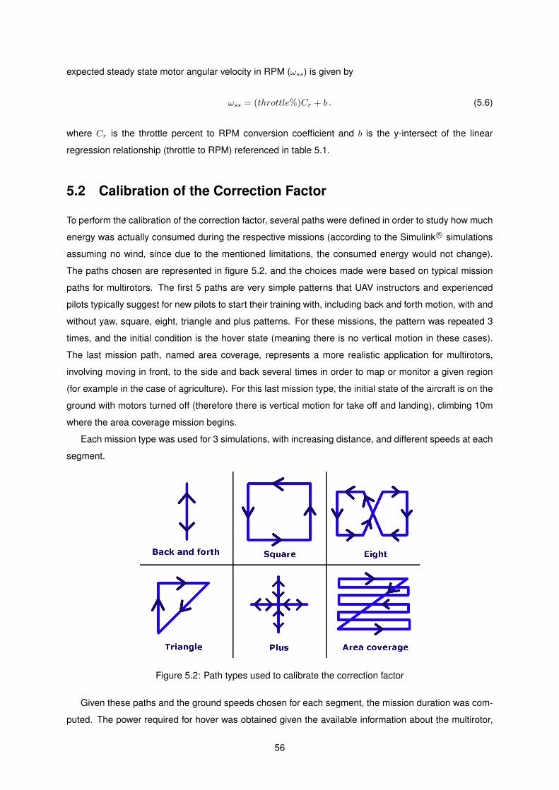
expected steady state motor angular velocity in RPM (ωss) is given by
ωss = (throttle%)Cr + b . (5.6)
where Cr is the throttle percent to RPM conversion coefficient and b is the y-intersect of the linear
regression relationship (throttle to RPM) referenced in table 5.1.
5.2 Calibration of the Correction Factor
To perform the calibration of the correction factor, several paths were defined in order to study how much
energy was actually consumed during the respective missions (according to the Simulink R© simulations
assuming no wind, since due to the mentioned limitations, the consumed energy would not change).
The paths chosen are represented in figure 5.2, and the choices made were based on typical mission
paths for multirotors. The first 5 paths are very simple patterns that UAV instructors and experienced
pilots typically suggest for new pilots to start their training with, including back and forth motion, with and
without yaw, square, eight, triangle and plus patterns. For these missions, the pattern was repeated 3
times, and the initial condition is the hover state (meaning there is no vertical motion in these cases).
The last mission path, named area coverage, represents a more realistic application for multirotors,
involving moving in front, to the side and back several times in order to map or monitor a given region
(for example in the case of agriculture). For this last mission type, the initial state of the aircraft is on the
ground with motors turned off (therefore there is vertical motion for take off and landing), climbing 10m
where the area coverage mission begins.
Each mission type was used for 3 simulations, with increasing distance, and different speeds at each
segment.
Figure 5.2: Path types used to calibrate the correction factor
Given these paths and the ground speeds chosen for each segment, the mission duration was com-
puted. The power required for hover was obtained given the available information about the multirotor,
56

from
T = W ⇒ Ti =W
4= 0.2557N , (5.7)
where Ti is the thrust produced by one motor,
ω =
√TiCt
, (5.8)
and
Tq = Cqω2 , (5.9)
resulting
Phover = Tqω = 84.94W . (5.10)
Knowing the power required to maintain flight in the equilibrium condition and the mission duration,
the initial estimate for the required propulsion energy to complete the mission (in this case from the start
to the end) can be obtained by integration according to equation (3.19).
From the consumed energy data obtained from the simulations and the initial estimate for the required
propulsion energy, the true correction factor for each path can be obtained, by rearranging equation
(3.20) and noting that ideally Eprop,t0→tf = Econs,t0→tf , resulting in
Cf =Econs,t0→tf
Eprop,t0→tf ,eq. (5.11)
For each path considered, its length, mission duration, the energy consumed, the corresponding
initial estimate and true correction factor are shown in table 5.2.
Given the limitations discussed in the previous section, the consumed energy obtained for each
mission is close to the value estimated by assuming the multirotor hovers for the whole duration of the
mission, since the control system only changes the angular velocity of the motors for attitude corrections,
and their value during linear motion is approximately equal to that of the hover condition. This means
that the true correction factor is in all cases close to 1. The plot of figure 5.3 shows the correction factor
as a function of mission duration, in which Cf is independent of mission duration. In reality, this is not
the result that should be expected since when moving at higher speeds the multirotor should consume
more energy compared to the hover condition, resulting in larger correction factors for longer missions.
With this in mind, the following discussion is simply meant to evaluate the consequences of choosing
different correction factors, and would not be valid for a real application until a better simulation model
was designed.
Assuming that Cf is approximately constant regardless of mission duration, its mean value would be
1.0226. Using this value for Cf , the consumed energy, the new propulsion required energy estimate and
the corresponding relative errors found for each path are shown in table 5.3.
Analysing the table, it is possible to note that the relative error is always inferior to 2.485%, which
means that if this multirotor has an actual endurance of 20 minutes, there would be an error of 30
57

Table 5.2: Simulation data obtained with Simulink R©
Path Totallength (m)
Missionduration (s) Econs,t0→tf (J) Eprop,eq,t0→tf (J) True Cf
Back and forth 1(no yaw) 180.0 62 5360.4 5267.3 1.0177
Back and forth 2(no yaw) 420.0 84 7354.8 7136.3 1.0306
Back and forth 3(no yaw) 1080.0 158 13815.0 13423.0 1.0292
Back and forth 1(with yaw) 180.0 87 7450.4 7391.2 1.0080
Back and forth 2(with yaw) 420.0 111 9629.6 9430.1 1.0212
Back and forth 3(with yaw) 1080.0 183 16304.0 15547.0 1.0487
Square 1 480.0 177 15241.0 15037.0 1.0136Square 2 1200.0 261 23005.0 22174.0 1.0375Square 3 2400.0 405 36054.0 34407.0 1.0479Eight 1 729.7 357 30576.0 30329.0 1.0081Eight 2 1942.9 507 43854.0 43073.0 1.0181Eight 3 3648.7 651 57646.0 55306.0 1.0423Triangle 1 409.7 177 15125.0 15037.0 1.0059Triangle 2 921.8 228 19679.0 19370.0 1.0160Triangle 3 1741.2 291 25868.0 24722.0 1.0464Plus 1 1200.0 327 28393.0 27781.0 1.0220Plus 2 2160.0 1167 99199.0 99144.0 1.0006Plus 3 2880.0 639 56364.0 54287.0 1.0383Area coverage 1 262.7 139 11909.0 11809.0 1.0085Area coverage 2 1018.9 347 29782.0 29480.0 1.0102Area coverage 3 3644.1 1063 90752.0 90308.0 1.0049
58

Table 5.3: Relative errors for the estimated propulsion required energy when Cf = 1.0226 and whenCf = 1.0487
Cf = 1.0226 Cf = 1.0487
Path Econs,t0→tf (J) Eprop,t0→tf (J) RelativeError (%) Eprop,t0→tf (J) Relative
Error (%)Back and forth 1(no yaw) 5360.4 5386.6 0.488 5523.8 3.048
Back and forth 2(no yaw) 7354.8 7297.9 0.774 7483.8 1.754
Back and forth 3(no yaw) 13815.0 13726.9 0.638 14076.6 1.893
Back and forth 1(with yaw) 7450.4 7558.6 1.452 7751.1 4.036
Back and forth 2(with yaw) 9629.6 9643.6 0.146 9889.3 2.696
Back and forth 3(with yaw) 16304.0 15899.0 2.484 16304.0 0
Square 1 15241.0 15377.5 0.895 15769.2 3.465Square 2 23005.0 22676.1 1.430 23253.7 1.081Square 3 36054.0 35186.0 2.407 36082.3 0.079Eight 1 30576.0 31015.7 1.438 31805.8 4.022Eight 2 43854.0 44048.3 0.443 45170.3 3.001Eight 3 57646.0 56558.2 1.887 57998.9 0.612Triangle 1 15125.0 15377.5 1.669 15769.2 4.259Triangle 2 19679.0 19808.6 0.658 20313.1 3.222Triangle 3 25868.0 25281.8 2.266 25925.7 0.223Plus 1 28393.0 28410.0 0.060 29133.7 2.609Plus 2 99199.0 101388.8 2.208 103971.4 4.811Plus 3 56364.0 55516.2 1.504 56930.3 1.005Area coverage 1 11909.0 12076.4 1.405 12384.0 3.989Area coverage 2 29782.0 30147.5 1.227 30915.4 3.806Area coverage 3 90752.0 92352.8 1.764 94705.2 4.356
59

Figure 5.3: True correction factor as a function of mission duration
seconds in the estimated endurance, which is a satisfactory value. However it is important to realise that
for some paths, this value for Cf results in an underestimation of the real energy consumption, which as
mentioned before is undesirable. To avoid this situation, using the maximum true correction factor found
(Cf = 1.0487), the new propulsion required energy estimates and the corresponding relative errors were
recomputed for each path, and the results are shown in the same table, in the two last columns.
As expected, for most paths the relative error increased compared to the previous case (using the
mean value for Cf ). Nonetheless the relative error obtained for the required propulsion energy estimate
while using the maximum true Cf found is inferior to 4.812%, meaning that for an actual endurance of 20
minutes, there would be an error of 58 seconds in the estimated endurance, which is still a good result.
With this new correction factor, there are no more underestimations of the actual consumed energy
(assuming no wind), however the path corresponding to the maximum correction factor, will have an es-
timate extremely close to the true energy consumption value. Also, for a real scenario, with an improved
aircraft control model, it would be important to add the influence of wind on the consumption. Addition-
ally, it would be wise to use a larger correction factor than the maximum one found or multiply it by a
safety factor since the accuracy of the estimation will be compromised in a real flight due to unforeseen
obstacle avoidance and the impossibility to predict the real wind conditions during the mission, which
would increase energy consumption. How much larger the correction factor would need to be relative
to the maximum one found in the simulations cannot be reliably discussed without real flight data for
comparison.
A different approach for obtaining the correction factor was considered, involving splitting it in hori-
zontal and vertical factors (each correcting for the energy spent in horizontal and vertical motion respec-
tively), as well as studying their dependence on airspeed and mission duration (assuming these are the
main factors affecting energy consumption). The results obtained are shown in figures 5.4 and 5.5.
The simulation points on these plots were obtained individually with a similar procedure as the correc-
tion factor introduced earlier (Cf ). In this case the paths used were straight lines, either in the horizontal
60
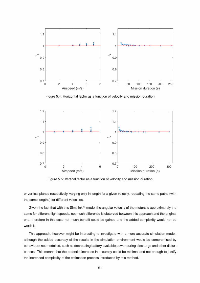
Figure 5.4: Horizontal factor as a function of velocity and mission duration
Figure 5.5: Vertical factor as a function of velocity and mission duration
or vertical planes respectively, varying only in length for a given velocity, repeating the same paths (with
the same lengths) for different velocities.
Given the fact that with this Simulink R© model the angular velocity of the motors is approximately the
same for different flight speeds, not much difference is observed between this approach and the original
one, therefore in this case not much benefit could be gained and the added complexity would not be
worth it.
This approach, however might be interesting to investigate with a more accurate simulation model,
although the added accuracy of the results in the simulation environment would be compromised by
behaviours not modelled, such as decreasing battery available power during discharge and other distur-
bances. This means that the potential increase in accuracy could be minimal and not enough to justify
the increased complexity of the estimation process introduced by this method.
61
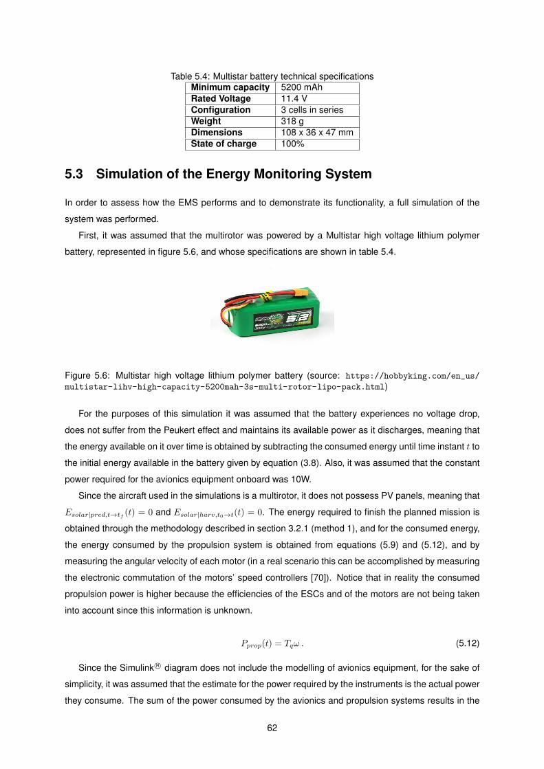
Table 5.4: Multistar battery technical specificationsMinimum capacity 5200 mAhRated Voltage 11.4 VConfiguration 3 cells in seriesWeight 318 gDimensions 108 x 36 x 47 mmState of charge 100%
5.3 Simulation of the Energy Monitoring System
In order to assess how the EMS performs and to demonstrate its functionality, a full simulation of the
system was performed.
First, it was assumed that the multirotor was powered by a Multistar high voltage lithium polymer
battery, represented in figure 5.6, and whose specifications are shown in table 5.4.
Figure 5.6: Multistar high voltage lithium polymer battery (source: https://hobbyking.com/en_us/
multistar-lihv-high-capacity-5200mah-3s-multi-rotor-lipo-pack.html)
For the purposes of this simulation it was assumed that the battery experiences no voltage drop,
does not suffer from the Peukert effect and maintains its available power as it discharges, meaning that
the energy available on it over time is obtained by subtracting the consumed energy until time instant t to
the initial energy available in the battery given by equation (3.8). Also, it was assumed that the constant
power required for the avionics equipment onboard was 10W.
Since the aircraft used in the simulations is a multirotor, it does not possess PV panels, meaning that
Esolar|pred,t→tf (t) = 0 and Esolar|harv,t0→t(t) = 0. The energy required to finish the planned mission is
obtained through the methodology described in section 3.2.1 (method 1), and for the consumed energy,
the energy consumed by the propulsion system is obtained from equations (5.9) and (5.12), and by
measuring the angular velocity of each motor (in a real scenario this can be accomplished by measuring
the electronic commutation of the motors’ speed controllers [70]). Notice that in reality the consumed
propulsion power is higher because the efficiencies of the ESCs and of the motors are not being taken
into account since this information is unknown.
Pprop(t) = Tqω . (5.12)
Since the Simulink R© diagram does not include the modelling of avionics equipment, for the sake of
simplicity, it was assumed that the estimate for the power required by the instruments is the actual power
they consume. The sum of the power consumed by the avionics and propulsion systems results in the
62

total consumed power, and by integrating between t0 and t it is possible to obtain the consumed energy.
The area coverage mission 2 was the mission chosen for the full system simulation (assuming no
wind), and the results obtained are represented in figures 5.7 through 5.9.
Figure 5.7: Estimate for the energy remaining at the end of the mission and its components
The qualitative analysis of figure 5.7 is promising. As the mission progresses the consumed energy
increases as expected, starting at 0J and ending with its maximum value; similarly, the estimate for the
required energy to complete the mission decreases over time, having its maximum value at t = 0s, and
reaching 0J at the end of the mission. Notice that the estimate for the required energy at t = t0 is almost
equal to the value of the consumed energy at t = tf , which indicates that the estimate for the required
energy is very satisfactory.
Figure 5.8 discriminates each of the energy required estimate components. The main contribution
to the expected energy required is that which is to be consumed by the propulsion system. This goes
in line with the fact that the power required for hover is 84.94W, while the power required to power the
onboard avionics was assumed to be only 10W. The variation in the required energy estimate due to
the changes in kinetic and potential energies over time is very small. A zoomed in version of this plot is
presented in figure 5.9.
The values of these variables are negative for the majority of the mission, since they represent the
change in potential or kinetic energy from the instant of calculation t until the end of the mission (in which
the altitude and velocity are both zero). The change in potential energy over time stays approximately
constant (with some variations due to altitude control imperfections) for the majority of the mission, since
the area coverage is performed at constant altitude. The change in kinetic energy oscillates between a
value of around -8J to 0J, since the UAV stops at every corner of the path to change its yaw and point in
the direction of the next track.
63

Figure 5.8: Estimate for the energy required to complete the mission and its components
Figure 5.9: Zoomed in plot of the change in potential energy and in kinetic energy (components of therequired energy)
The energy available in the energy sources (battery and mechanical energy in this case) decreases
over time as expected. From its initial value it decreases around 35kJ until the end of the mission,
around the same amount of total consumed energy, which makes sense. Figure 5.10 represents the
components of the energy available in the sources over time. As expected, most of the energy available
in the sources corresponds to the energy available in the battery. The potential energy can be seen
64

in greater detail in figure 5.11, and it increases while the multirotor is climbing, stays approximately
constant during the area coverage operation and decreases during landing, as expected. The kinetic
energy oscillates, which can be explained by the acceleration and deceleration of the aircraft during its
back and forth motion.
Figure 5.10: Energy available in the energy sources over time and its components
Figure 5.11: Zoomed in plot of the potential and kinetic energy over time (components of the energyavailable in the sources)
The estimate for the energy remaining in the energy sources at the end of the mission should, ideally,
65

be a straight line (constant value over time), meaning that at any instant, during the course of the mission,
it is possible to predict the final state of the energy sources. This parameter is the most important in the
context of the energy monitoring system. Its analysis is what allows the pilot, or the mission planning
module to understand whether or not there will be enough energy available to finish the planned mission.
If the value of Erem,tf drops below zero at any moment, it means the UAV will not have enough energy
to finish the planned mission successfully, and the mission should be changed accordingly. However,
for a real scenario, a safety threshold must be defined in order to avoid accidents, and if Erem,tf drops
below this value, the mission should be immediately replanned.
From the results shown in figure 5.7, it appears that the energy remaining estimate is approximately
constant, at around 84% of the total energy of the battery, meaning this mission is feasible. However it
is possible to observe a slight increase over time in figure 5.12, of around 1100J.
Figure 5.12: Estimate for the energy remaining at the end of the mission
The reason for this increase is due to the fact that the required energy is an overestimate (the
maximum value of the true Cf found in section 5.2 was used) of the amount of energy that will actually
be consumed in the remainder of the mission, leading to a rate of consumption that is in reality lower
than that which was estimated. Remembering equations (2.2) and (2.1), since Ereq,t→tf (t) decreases
faster than Econs,t0→t(t) increases, this leads to an overall increase in Erem,tf (t).
66

Chapter 6
Simulations Based on Experimental
Data for the LEEUAV
In this chapter, pre-flight mission estimates are obtained and discussed for the case of the LEEUAV,
based on experimental data. Two approaches to estimate the required energy to complete the mission
(methods 2 and 3 from section 3.2.1) are compared, one based on propeller experimental data provided
in tables, which, given the required thrust and required airspeed, provide the power coefficient and angu-
lar velocity of the propellers for that flight condition, and another based on an experimental relationship
between airspeed and required electric power. The influence of wind on the performance of the energy
monitoring system is also investigated.
The reason why only a pre-flight mission energy assessment was carried out, instead of performing
the study for an entire mission, was due to the fact that it was not possible to perform flight tests to gather
data, and a LEEUAV control and guidance model was not available to simulate a flight.
The first section introduces the aircraft’s relevant parameters, the chosen missions to evaluate the
pre-flight energy balance and the algorithm used for the simulations. The second section focuses on
validating the correct functioning of the simulation tool, by studying the effects of wind on the required
energy to complete the mission, and comparing both methods used to arrive at this estimate. The last
section presents the simulation results obtained for both missions, for different days of the year with an
arbitrary wind speed profile, analysing how the remaining energy estimate is helpful in understanding if
a planned mission can be successfully completed.
6.1 Aircraft, Mission and Algorithm Descriptions
The aircraft used in this chapter’s simulations was the LEEUAV. Table 6.1 highlights relevant data about
this aircraft.
The mission profiles of the two missions used to perform the simulations are shown in figures 6.1
and 6.2, along with their respective ground speed profiles, while the waypoints that define each mission,
as well as the total ground distance covered in each one are shown in table 6.2. The first is a simple
67

Table 6.1: Relevant LEEUAV data [69]Maximum take-off weight 54.129 NWing area 1.490 m2
Propeller diameter 0.4064 mLift to drag ratio 17.43PV panel efficiency 22.5%PV panel area 0.792 m2
Battery nominal charge 10000 mAhMax. operating altitude 718 mTake-off distance 10 mMin. landing distance 40 mTake-off speed 6.94 m/sMax. vertical speed 2 m/sCruise speed 7.8 m/sMax. speed 26 m/sStall speed 6.5 m/sMax. landing speed 10 m/sMax. acceleration (assumed) 1 m/s 2
Max. decceleration (assumed) 0.5 m/s 2
Commands range 80 kmFirst person view range 10 kmTelemetry range 2 kmPower required for avionics 28.04 W
climb, cruise and descent mission, while the second is slightly more complex. The take-off and landing
segments were not considered, in order to simplify the simulations and due to the short amount of time
spent in these stages, which in turn results in a small change in the energy consumed.
Figure 6.1: Mission 1 profile and respective ground speed profile
In both missions the aircraft always travels in approximately the same direction. The reason for
this choice was to simplify the study on the effect of wind velocity on the required energy to complete
the mission, by assuming it has a constant direction. Additionally it was also assumed that the wind
velocity has no vertical component. For a simulation of a real flight it would be necessary to obtain a
map with an estimate for the wind velocity in the area where the mission is to be performed (the wind
spatial distribution). However for the purposes of this thesis a temporal distribution of wind is used
instead, which, knowing the desired ground speed for the mission, could be obtained from the spatial
68

Table 6.2: Set waypoints and total length for each missionMission 1 Mission 2
Waypoints
W1: 38◦43’54.53”N09◦11’17.71”W
W1: 41◦11’23.28”N08◦37’05.10”W
W2: 38◦41’38.22”N09◦08’28.37”W
W2: 41◦08’42.24”N08◦36’37.61”W
W3: 38◦36’08.69”N09◦00’49.38”W
W3: 41◦06’00.81”N08◦36’15.78”W
W4: 38◦31’17.39”N08◦54’17.75”W
W4: 41◦04’47.19”N08◦36’03.34”W
- W5: 41◦03’10.54”N08◦35’45.15”W
- W6: 40◦59’06.16”N08◦34’54.13”W
- W7: 40◦58’17.54”N08◦34’48.39”W
- W8: 40◦56’12.06”N08◦34’35.92”W
Total grounddistance 33.970 km 28.326 km
distribution.
Figure 6.2: Mission 2 profile and respective ground speed profile
The MATLAB R© algorithm used for this chapter’s simulations is represented in figure 6.3. The set
waypoints for the aircraft to follow are provided in a file, which is then read, and the waypoints saved
in a matrix. The initial position is set equal to the first waypoint, and the climb angle, the components
of ground speed and acceleration in the inertial reference frame (ECEF - Earth Centered Earth Fixed)
are obtained. The initial energy available in the energy sources is then calculated and the cycle begins
by accumulating (every iteration) the predicted solar energy harvested and the energy expected to be
required during the time step tstep chosen for the simulation.
If the aircraft is not yet within range of the next waypoint (dw, defined in equation (6.1)), the position
is updated by converting the aircraft’s position from geodesic to ECEF coordinates [71] (assuming the
WGS-84 reference ellipsoid), using equation (3.31) and converting the result back to geodesic coordi-
nates (using the same reference ellipsoid and the Heikkinen method [71]). The velocity and acceleration
69

Figure 6.3: MATLAB R© algorithm used to perform the simulations
are also updated using the equations of linearly accelerated uniform motion. The instant of prediction is
then incremented by the step value defined for the simulation, and the aircraft’s position is checked to
evaluate whether it is in range of the next waypoint or not, and a flag is activated (or not). After this, the
cycle repeats.
dw = vGtstep , (6.1)
where dw is the distance between the aircraft predicted position and the next waypoint.
In case the aircraft is in range of the next waypoint, the time interval required to reach it is obtained
such that the position, velocity and acceleration can be correctly updated. Afterwards, if this completed
mission segment was not the last one, the climb angle and the components of velocity and acceleration
in the ECEF reference frame are obtained for the next segment, and the position is yet again updated.
70

Table 6.3: Required energy to complete the mission (in kJ) under different wind conditionsWind speed
2 m/s 0 m/s -2 m/s
Mission 1 Method 2 951.841 694.330 679.384Method 3 412.042 333.922 300.820
Mission 2 Method 2 943.639 711.630 696.149Method 3 397.815 336.495 310.557
If however that was the last mission segment, the cycle ends, the predicted solar energy and required
energy are accumulated once more (during the time interval required to reach the last waypoint, from
the previous predicted position), the predicted remaining energy at the end of the flight is calculated and
the algorithm ends.
6.2 Algorithm Qualitative Validation and Method Comparison
Using the previously described algorithm, the required energy to complete both missions is obtained
with methods 2 and 3 of section 3.2.1 under different wind speeds, and the results are shown in table
6.3. The wind speeds are assumed constant during the whole mission and in the same direction the
aircraft is travelling, and the convention used is positive for headwind and negative for tailwind. The
reason for these choices was simply to evaluate if the algorithm was working properly, which is verified
by noticing that when the aircraft faces headwind the required energy to complete the mission is larger
than when there is no wind, which in turn is larger than when there is tailwind, for both missions and with
both methods.
Another noteworthy fact is the large discrepancy between the obtained required energy estimates of
both methods, under the same conditions. It is important to be aware that the estimates obtained with
method 3 are based on an experimental characterization of the aircraft’s electric power requirements
at different airspeeds valid for cruise. In the simulations this experimental characterization is used to
estimate not only the power requirements during cruise, but also those for the climb segment, which
requires much more power to fly than the cruise segment. In an attempt to mitigate the estimation error
for the climb segment obtained with this method, the following correction is made for this mission stage,
Pclimb = Pcruise +WvG sin(γ)
ηprop, (6.2)
where Pclimb is the required power for the climb segment, Pcruise is the required power for the cruise
segment (taken directly from the plot of figure 3.7), and the logic behind the last term is analogous to
the approach used in equation (2.16) but for vertical motion. Even with this correction there is still a
discrepancy between the estimates obtained with both methods considered in this chapter.
According to [50] which describes the design process of the LEEUAV, estimates are provided for the
propulsion system efficiency and for the required propulsion electrical power to fly at different mission
stages. Notice that these estimates do not include the power required by the avionics, and they are
shown in table 6.4. Figure 6.4 shows a comparison between the estimated required electrical propulsion
71

Table 6.4: Propulsion system efficiency and required propulsion electric power estimates for flight duringdifferent stages for the LEEUAV [50]
ηprop (%) Pel (W)Take-Off 15.9 451.2Climb 22.4 444.7Cruise 38.2 46.7Descent - 0
power obtained with both methods for mission 1 (without considering wind).
Figure 6.4: Required electrical propulsion power for both methods during mission 1 without wind
Since the data available for method 3 is most reliable when estimating the required electrical propul-
sion power for the cruise segment, both methods will be compared during this stage. Using method 2
results in an estimated required electric power for cruise of 132.8 W, while with method 3 the result is
64.4 W. This means that method 2 overestimates the result obtained from method 3 by approximately
106% which is a large difference.
During climb (assuming γ = 5◦), method 2 outputs a required electrical propulsion power between
561.4 W and 595.2 W (varying due to the change in air density during climb). Compared to the estimate
provided in reference [50] this is an overestimate of around 30% (on average), which is still a relatively
large value, although a better result compared to a relative error of approximately 44.4% obtained by
using method 3 (required electric propulsion power during climb of 247.1 W). The descent segment
requires no propulsion power since it is assumed the aircraft glides during descent until it lands. It is
important to note however that the climb conditions considered in the estimate provided in reference
[50] are unknown, thus this comparison is only useful to establish a point of reference for the power
requirements of the climb stage, and not for an accurate quantitative comparison.
Although the errors found are not satisfactory, this does not necessarily mean that the proposed
methods should be discarded. These results allow, however, to conclude that these methods are sensi-
tive to the quality of the data available to perform the estimates.
Estimates with method 2 are heavily dependent on the tabled performance parameters of the pro-
pellers used. The tables available for these simulations were obtained from manufacturer data, which
in turn was obtained with simulation software. This eventually will lead to discrepancies between the
72
Table 6.5: Wind time profile considered in the simulationsWind speed (m/s) 1.2 0.8 1.9 1.5 0.3 0.7 0.6 1Mission instant (s) 0 600 1200 1800 2400 3000 3600 4200
expected performance and the actual performance of the propellers. Even if the manufacturer data was
obtained through experimental characterization, this would not suffice to characterize every propeller
with the same diameter and pitch, since this is a simplistic way to characterize a set of propellers. To ob-
tain better tabled parameter data as a function of required thrust and airspeed, experimental tests should
be performed with the specific propellers to be used with the aircraft being simulated. Additionally, the
required thrust is estimated based on the data of figure 3.5, which represents the relationships between
lift coefficient and angle of attack and lift coefficient and drag coefficient, which were obtained through
simulation software, which again may introduce additional errors to the estimates obtained. Lastly the
two-dimensional balance of forces considered is a simplification of a tri-dimensional problem, thus in-
troducing additional error, and the equation used to obtain the mechanical power of the propeller is an
approximation based on an expression valid for helicopters in hover.
Estimates with method 3 rely on experimental characterization of the required electric power as a
function of airspeed and, in this case, this data was only available for the cruise condition, resulting in
low quality estimates for the required electric power for climb despite the correction proposed.
6.3 Simulation Results and Analysis
In a real scenario, the simulations discussed in this section would evaluate the capacity of the LEEUAV to
perform the previously mentioned missions before the mission starts, thus it is an offline energy balance
assessment. The reason why only pre-mission estimates were studied was due to the fact that it was
not possible to perform flights with the aircraft to obtain the real time data measurements required to
compute the consumed energy term.
The capacity of the LEEUAV to complete both missions was simulated for 2 different days (Summer
and Winter Solstices), with different starting hours. The arbitrary temporal wind profile considered is
shown in table 6.5, and it was assumed the wind velocity has the same direction of the aircraft’s motion,
with the signal convention introduced in the previous section. In the same table, the mission time instants
correspond to the moments when the wind speed changes to the value in the line above.
The influence of the simulation time step on the results was also investigated. Table 6.6 shows the
initial energy available in the sources and the required energy for both missions and both methods under
the mentioned wind conditions for variable time steps. These terms do not depend on the day and hour
the mission is performed.
The difference between the initial energy available in the sources of both missions results from the
difference in altitude between the take-off and landing points.
For different days of the year (day 172 - Summer Solstice, and day 355 - Winter Solstice) and different
starting hours for each mission, the expected solar energy harvest and corresponding remaining energy
73

Table 6.6: Required energy obtained for different simulation time steps and initial energy available in thesources for both missions
Ereq (kJ)Esources,t0 (kJ)
tstep = 1s tstep = 10s tstep = 20s
Mission 1 Method 2 832.871 836.575 836.826 408.911Method 3 380.962 382.642 382.923
Mission 2 Method 2 819.755 822.504 822.825 397.056Method 3 368.774 369.975 370.255
Table 6.7: Solar energy predicted harvest, remaining energy estimates and correspondent relative errorsrelative to the result with tstep = 1s
Mission 1 Mission 2
Day: 172Hour: 9h
Day: 172Hour:15:45h
Day: 355Hour: 9h
Day: 172Hour: 9h
Day: 172Hour:15:45h
Day: 355Hour: 9h
Esolar|pred(kJ)
tstep = 1s 625.735 427.639 262.425 514.367 368.894 191.382tstep = 10s 627.213 428.649 263.041 515.298 369.627 191.706tstep = 20s 628.846 429.768 263.721 516.902 370.781 192.299
Method 2:Erem
(kJ)
tstep = 1s 201.775 3.679 -161.535 91.668 -53.805 -231.317tstep = 10s 199.549 0.985 -164.623 89.850 -55.821 -233.742tstep = 20s 200.931 1.853 -164.194 91.133 -54.988 -233.470
Method 3:Erem
(kJ)
tstep = 1s 653.683 455.587 290.373 542.649 397.176 219.664tstep = 10s 653.482 454.917 289.310 542.379 396.708 218.787tstep = 20s 654.834 455.756 289.709 543.702 397.581 219.099
Method 2:RelativeError (%)
tstep = 10s 1.103 73.235 1.912 1.983 3.747 1.048tstep = 20s 0.418 49.639 1.646 0.583 2.198 0.931
Method 3:RelativeError (%)
tstep = 10s 0.031 0.147 0.366 0.050 0.118 0.399tstep = 20s 0.176 0.037 0.229 0.194 0.102 0.257
estimates are obtained for both missions and for different time steps, and the results are presented in
table 6.7.
There are three main conclusions to be drawn from this table. First it is possible to observe that
during the Summer Solstice more solar energy is expected to be harvested compared to the Winter
Solstice when the mission begins at the same hour, which makes sense. Also, on the same day more
energy is expected to be collected if the mission starts in the morning than later in the afternoon, which
is also a result to be expected.
Secondly, the remaining energy term provides insight into what missions and under which conditions
are possible to complete safely. With the previously mentioned temporal wind distribution, and using
method 2 to calculate the required energy to complete the mission, it is predicted that the first mission
can be completed safely in the Summer Solstice if it starts at 9h, and the battery would still have around
49.9% of its total energy at the end. If the mission starts at 15:45h however, the battery is predicted to
finish the mission with only around 0.2% of its total energy, which is a value low enough to raise safety
concerns, and the mission should be replanned. During the Winter Solstice, the value of remaining en-
ergy is negative, meaning that the battery does not have enough energy to complete this mission, since
not enough solar energy would be collected to compensate the amount consumed. A similar analysis
could be performed for mission 2. If method 3 is used instead to calculate the required propulsion power,
74

Table 6.8: Mission duration and calculation time interval for the remaining energy estimatesMission 1 Mission 2
tstep = 1s tstep = 10s tstep = 20s tstep = 1s tstep = 10s tstep = 20sExpected mission
duration (s) 3811 3811 3811 3194 3191 3191
Calculation timeinterval (s) -
Method 2118.563 11.613 7.146 135.778 13.587 6.740
Calculation timeinterval (s) -
Method 32.858 0.677 0.688 2.337 0.797 0.724
then the conclusion would be that both these mission could be completed safely in any of the conditions
considered. In reality, this probably would not be true since given the available data, the power require-
ments for climb are underestimated by this method. With better data available, this method would be
more useful and provide more accurate remaining energy estimates.
Finally, the last conclusion to be drawn is that given the algorithms developed, method 3 calculates
the remaining energy estimate much faster than method 2, as evidenced by table 6.8, while this differ-
ence is especially notorious for smaller simulation time steps. The reason for this is the fact that in the
case of method 3 the required electric power is directly related to airspeed, while in the case of method
2 it is necessary to search the propeller performance tables for the right parameters given the required
thrust and airspeed. Therefore if obtaining a fast remaining energy estimate is crucial, it may be worth
investing in calibrating method 3 with more accurate data not just for cruise but also for climb. In longer
missions method 3 would also dramatically outperform method 2 in terms of computation speed.
Additionally, by increasing the simulation time step from 1 to 20 seconds, the relative error of the
remaining energy estimate, compared to the value obtained with a 1 second time step, remains relatively
small (below 4%). An exception occurs for the afternoon mission 1 during the Summer Solstice, but this
is due to the low absolute value of the remaining energy estimates obtained in this case. Increasing
the simulation time step reduces the time required to perform the estimates, which is desirable as long
as the relative error does not increase too much, since if the estimation process is too long, it may no
longer be relevant by the time it is finished. The choice of time step would depend on the mission, and
longer missions would certainly benefit from larger time steps in terms of computational speed.
Notice however that in this problem the conditions are quasi-static, and for for this reason there is
more freedom of choice for the simulation time step without significant consequences, which would not
be the case if the problem parameters suffered larger and more frequent variations over time, in which
case a smaller value would have to be used to avoid compromising the accuracy of the estimates.
It is important to keep in mind that computation time depends on the system running the simulations
and can vary depending on CPU load, which justifies why in some situations, although the time step is
larger, the computation time is longer. All simulations were performed on a system with 4GB of RAM
(random access memory) and a CPU running at 2.4GHz.
75

76

Chapter 7
Conclusions
In this work, an EMS for the Drones Safe Flight project was proposed, which evaluates the past and
future energy balance of the onboard energy sources of the aircraft. The key terms of the balance of
forces are the initial total energy available in the sources at the start of the mission, the consumed and
the solar harvested energy, which are measured in real time with appropriate sensors, the solar energy
expected to be harvested in the remainder of the mission, based on a solar irradiation model from the
literature, and the required energy to complete the mission, for which three different estimation methods
were discussed.
The performance of each method and of the overall EMS was discussed and qualitatively validated.
The first method to obtain an estimate for the required energy to complete the mission was based on the
idea of having a base energy estimate corrected by an empirical factor. The correction factor was cali-
brated using a Simulink R© model of a multirotor available on the internet to simulate the base prediction
and the consumed energy for six different missions types. In this work, the approach discussed attempts
to produce a general correction factor for the multirotor in study, although in hindsight this would most
likely produce low accuracy results. The correction factor should be calibrated pre-mission, for a specific
planned mission and predicted environmental conditions, being invalid for other conditions. By simulat-
ing the mission with slight variations in the predicted environmental conditions, some correction factors
would be obtained and the maximum found should be the one used to predict the required energy to
complete the mission, preventing safety hazards due to insufficient energy, leading to earlier mission re-
planning, and predicting deficiencies in energy resources ahead of time. However, severe overestimates
can also cripple the range of the UAV, therefore making the calibration of the correction factor one of
the most challenging and critical parts of the design of the EMS. Since the simulation tool used did not
account for the effects of wind on the dynamics of the aircraft, if it was used to simulate a real scenario,
a larger correction factor would have to be used, to avoid underestimating the energy requirements for
the mission. Additionally, a safety factor should also be multiplied to the predicted energy requirements
for the mission, whether or not wind is taken into account in the simulations, to account for unforeseen
disturbances, the impossibility to predict the real wind conditions and unexpected obstacle avoidance
manoeuvres.
77

Another proposed method to estimate the mission energy requirements is based on tabled relation-
ships between the required thrust for a given flight condition and the performance of propellers, the
polar curve of the aircraft and the relationship between lift coefficient and angle of attack. Propeller
manufacturer data was used in the simulations based on this method, and was concluded that it was not
accurate enough for real applications, overestimating the power requirements for cruise by as much as
106%, and therefore an experimental characterization of the particular propellers used on the aircraft is
required to obtain higher quality estimates. The polar curve and the curve describing the relationship be-
tween lift coefficient and angle of attack used were obtained through software tools, potentially being an
additional source of error. The balance of forces used in this method is a bi-dimensional approximation
of a tri-dimensional problem, adding extra error, as well as the expression used to obtain the propeller
mechanical power, which is based on an equation valid for helicopters in hover.
The last method proposed to estimate the required energy to complete the mission is based on
experimental characterization of the electrical power required to operate the aircraft during cruise as
a function of airspeed. This method is highly accurate in predicting the energy requirements for the
cruise stage, but since only data for cruise was available the power requirements for the climb stage are
underestimated despite the correction introduced for required power estimates during this stage. With
a similar experimental characterization for the take-off and climb stages, more accurate estimates could
easily be obtained.
These three proposed methods are highly sensitive to the quality of the data and tools available. The
biggest challenge found in this work was obtaining appropriate data and simulation tools to validate the
proposed methods. The design of a control system for an UAV was outside the scope of this thesis,
and obtaining access to a complete Simulink R© control and guidance diagram was difficult. The best
alternative found still had some flaws. Attitude and especially guidance control, could be improved for
better system modelling. It was also not possible to perform flight tests with the LEEUAV to obtain
better quality data to fit the purpose of the last two methods discussed, thus only data from previous
works was available. The 3 proposed methods to estimate the required energy by the propulsion system
were simply workarounds the limitation of not having a control and guidance model for the LEEUAV
available, leading to underwhelming results. With this in mind the results obtained, although qualitatively
satisfactory, should be considered with some criticism.
Clearly there is much room for improvement in future work, although this thesis attempts to assert the
importance of the remaining energy estimation for the safety of low-cost UAVs. This parameter is useful
when trying to predict mission feasibility, enabling better energy awareness during mission planning, and
contributing to an online assessment of energy resources and mission energy requirements to enhance
safety and prevent accidents. However it does not take into account situations where, for example, a
very demanding climb condition would exhaust the battery’s energy, even though if the flight continued
the total energy balance could be positive since in cruise excess solar energy could be collected to
recharge the battery. A failsafe to account for situations like these would have to be implemented, for
example by breaking down the energy balance problem into subproblems for each mission segment,
and if in any segment the remaining energy at the end of the segment was predicted to be negative then
78

the mission would not be feasible.
Another aspect that is important to consider is the computation time of the energy remaining estimate.
This calculation must be performed fast enough to keep up with sensor readings, in order for the result
to be relevant. According to the simulations performed, as long as a large enough simulation time step
is chosen, the required calculations for arriving at this estimate are doable in a reasonable time frame
and no problems should be expected, however it is something worth taking into account before real flight
testing. The simulation time step cannot be too large however, to avoid degrading the accuracy of the
estimates, thus the right balance between computation time and result accuracy has to be found.
7.1 Achievements
The goal of this thesis was to design a system capable of outputting an estimate for the final state of the
energy sources onboard the aircraft, updated regularly during the mission. Only a couple of works with
similar goals are discussed in the literature, not taking into account the influence of wind on the future
energy requirements of the aircraft.
Although more testing and improvements need to be done on the proposed system, the initial goal
was accomplished and solid foundations for future work were qualitatively validated, and considering
the lack of embedded safety systems onboard most low-cost UAVs, the industry’s focus on safety and
the lack of similar works discussed in the literature, the contribution of this thesis is valuable, introducing
three methods not considered previously for estimating the energy requirements of a given mission.
7.2 Future Work
This thesis established the foundations for the development of an EMS for the Drones Safe Flight project,
however there are still improvements and future work required. Moving forward, the first step should be
to focus on the crucial step of estimating the required energy to complete the mission.
The correction factor method relies on an accurate simulation model for the aircraft on which the EMS
is to be implemented, and as such developing this tool should be a priority, and it should include guidance
and control systems with good performance and the influence of wind on its dynamics. Additionally,
a more realistic battery model than the one suggested in this work, including the Peukert effect and
voltage and available power drop as it discharges, would also benefit the project. Modelling the power
consumption of the onboard avionics equipment could also lead to improved simulation accuracy.
The second method is based on tabled relationships between required thrust for manoeuvres and
the corresponding propeller angular velocity and power coefficient, as well as the polar curve for the
aircraft and the relationship between lift coefficient and angle of attack. Improving the reliability of this
method depends on how accurate the tabled information is. Therefore, experimental characterization of
the particular propellers used on the aircraft should be obtained, as well as an experimental polar curve
and lift coefficient as a function of angle of attack curve from wind tunnel tests.
79

Finally for the third method, performing flight tests and recording electrical power required as a func-
tion of airspeed for each flight stage, and not only for cruise, would lead to better estimates when using
this method.
Flight tests should follow in order to compare the performance of each alternative presented to cal-
culate the required energy to complete the mission, and verify the performance of the EMS, as well as
potentially improving the calibration of the correction factor obtained through simulations even further
with more data available.
Further in the future, the EMS, the mission planning module and the obstacle detection and avoid-
ance modules should be integrated together and the full system’s performance assessed on ground and
flight tests to demonstrate an increase in safety in low-cost UAVs, as this is the main goal of the Drones
Safe Flight project.
80

Bibliography
[1] S. G. Gupta, M. M. Ghonge, and P. M. Jawandhiya. Review of Unmanned Aircraft System (UAS).
International Journal of Advanced Research in Computer Engineering & Technology, 2(4):1646–
1658, 2013.
[2] A. C. Marta, A. Moutinho, and P. Gamboa. Drones Safe Flight: On Addressing Operational Safety
For Low Cost Small Drones. In Mechanical Engineering Conference, June 2016.
[3] K. Anderson and K. J. Gaston. Lightweight unmanned aerial vehicles will revolutionize spatial ecol-
ogy. Frontiers in Ecology and the Environment, 11(3):138–146, April 2013. doi:10.1890/120150.
[4] C. D. Franco and G. Buttazzo. Coverage path planning for UAVs photogrammetry with energy and
resolution constraints. Journal of Intelligent & Robotic Systems, 83(3):445—-462, September 2016.
doi:10.1007/s10846-016-0348-x.
[5] P. Miller. Design of a remote person view system for a long range UAV. Master’s thesis, Instituto
Superior Tecnico, June 2015.
[6] G. L. Dillingham. Unmanned Aircraft Systems: Use in the National Airspace System and the Role of
the Department of Homeland Security. Technical report, United States Government Accountability
Office, July 2012. GAO-12-889T.
[7] X. Yu and Y. Zhang. Sense and Avoid Technologies with Applications to Unmanned Air-
craft Systems: Review and Prospects. Progress in Aerospace Sciences, 74:152–166, 2015.
doi:10.1016/j.paerosci.2015.01.001.
[8] F. Duchon, A. Babinec, M. Kajan, P. Beno, M. Florek, T. Fico, and L. Jurisica. Path Plan-
ning with Modified A Star Algorithm for a Mobile Robot. Procedia Engineering, 96:59–69, 2014.
doi:10.1016/j.proeng.2014.12.098.
[9] M. Kothari and I. Postlethwaite. A Probabilistically Robust Path Planning Algorithm for UAVs Using
Rapidly-Exploring Random Trees. Journal of Intelligent & Robotic Systems, 71(2):231–253, August
2013. doi:10.1007/s10846-012-9776-4.
[10] E. I. Grøtli and T. A. Johansen. Path Planning for UAVs Under Communication Constraints Us-
ing SPLAT! and MILP. Journal of Intelligent & Robotic Systems, 65(1):265–282, January 2012.
doi:10.1007/s10846-011-9619-8.
81

[11] G.-C. Luo, J.-Q. Yu, Y.-S. Mei, and S.-Y. Zhang. UAV Path Planning in Mixed-Obstacle Environment
via Artificial Potential Field Method Improved by Additional Control Force. Asian Journal of Control,
17(5):1600–1610, October 2014. doi:10.1002/asjc.960.
[12] Z. Lihua, C. Xianghong, and Y. Fuh-Gwo. A 3D Collision Avoidance Strategy for UAV with Physical
Constraints. Measurement, 77:40–49, 2016. doi:10.1016/j.measurement.2015.09.006.
[13] V. Bonnin, E. Benard, J. M. Moschetta, and C. A. Toomer. Energy-Harvesting Mechanisms for
UAV Flight by Dynamic Soaring. International Journal of Micro Air Vehicles, 7(3):213–229, 2015.
doi:10.1260/1756-8293.7.3.213.
[14] S. Hosseini, R. Dai, and M. Mesbahi. Optimal Path Planning and Power Allocation for a Long
Endurance Solar-Powered UAV. In American Control Conference, June 2013.
[15] B. Saha, E. Koshimoto, C. C. Quach, E. F. Hogge, T. H. Strom, B. L. Hill, S. L. Vazquez, and
K. Goebel. Battery health management system for electric UAVs. In Aerospace Conference, 2011
IEEE. IEEE, March 2011. doi:10.1109/AERO.2011.5747587.
[16] A. M. Shevchenko. Energy-based approach for flight control systems design. Automation and
Remote Control, 3(74):372–384, March 2013. doi:10.1134/S0005117913030041.
[17] A. M. Shevchenko and G. N. Nachinkina. Energy method of safe aircraft brak-
ing forecasting. Automation and Remote Control, 76(9):1664–1672, September 2015.
doi:10.1134/S000511791509012X.
[18] G. Gramajo and P. Shankar. Path-planning for an unmanned aerial vehicle with energy constraint
in a search and coverage mission. In Green Energy and Systems Conference. IEEE, November
2016. doi:10.1109/IGESC.2016.7790077.
[19] Y. Huang, H. Wang, and P. Yao. Energy-optimal path planning for solar-powered UAV with
tracking moving ground target. Aerospace Science and Technology, 53:241—-251, June 2016.
doi:10.1016/j.ast.2016.03.024.
[20] G. Xian-Zhong, H. Zhong-Xi, G. Zheng, L. Jian-Xia, and C. Xiao-Qian. Energy management strat-
egy for solar-powered high-altitude long-endurance aircraft. Energy Conversion and Management,
70:20–30, June 2013. doi:10.1016/j.enconman.2013.01.007.
[21] P. Oettershagen, A. Melzer, T. Mantel, K. Rudin, T. Stastny, B. Wawrzacz, T. Hinzmann,
K. Alexis, and R. Siegwart. Perpetual flight with a small solar-powered UAV: Flight results,
performance analysis and model validation. In Aerospace Conference. IEEE, March 2016.
doi:10.1109/AERO.2016.7500855.
[22] L. Karunarathne, J. T. Economou, and K. Knowles. Power and Energy Management Sys-
tem for Fuel Cell Unmanned Aerial Vehicle. In Proceedings of the Institution of Mechani-
cal Engineers Part G Journal of Aerospace Engineering, volume 226, pages 437–454, 2012.
doi:10.1177/0954410011409995.
82

[23] K. Dorling, J. Heinrichs, G. G. Messier, and S. Magierowski. Vehicle routing problems for drone
delivery. IEEE Transactions on Systems, Man, and Cybernetics: Systems, 47(1):70–85, January
2017. doi:10.1109/TSMC.2016.2582745.
[24] O. Atlam and M. Kolhe. Performance evaluation of directly photovoltaic powered DC PM (direct
current permanent magnet) motor – propeller thrust system. Energy, 57:692—-698, August 2013.
doi:0.1016/j.energy.2013.05.052.
[25] M. Hepperle. Electric flight – potential and limitations. Technical report, Institute of Aerodynamics
and Flow Technology, German Aerospace Center, 2012. NATO unclassified document.
[26] L. W. Traub. Range and endurance estimates for battery-powered aircraft. Journal of Aircraft, 48
(2):703–707, April 2011. doi:10.2514/1.C031027.
[27] T. Donateo, A. Ficarella, L. Spedicato, A. Arista, and M. Ferraro. A new approach to calculating
endurance in electric flight and comparing fuel cells and batteries. Applied Energy, 187:807–819,
February 2017. doi:10.1016/j.apenergy.2016.11.100.
[28] M. Gatti, F. Giulietti, and M. Turci. Maximum endurance for battery-powered rotary-wing aircraft.
Aerospace Science and Technology, 45:174–179, September 2015. doi:10.1016/j.ast.2015.05.009.
[29] J. F. Roberts, J.-C. Zufferey, and D. Floreano. Energy management for indoor hovering robots. In
2008 IEEE/RSJ International Conference on Intelligent Robots and Systems. IEEE, Semptember
2008. doi:10.1109/IROS.2008.4650856.
[30] M. Gatti. Design and prototyping high endurance multi-rotor. Master’s thesis, University of Bologna,
2015.
[31] T. Chang and H. Yu. Improving electric powered uavs endurance by incorporating battery dumping
concept. Procedia Engineering, 99:168–179, 2015. doi:10.1016/j.proeng.2014.12.522.
[32] M. Ceraolo and G. Pede. Techniques for estimating the residual range of an electric vehicle. IEEE
Transactions on Vehicular Technology, 50(1):109–115, January 2001. doi:10.1109/25.917893.
[33] Y. Wang, C. Zhang, and Z. Chen. An adaptive remaining energy prediction approach for
lithium-ion batteries in electric vehicles. Journal of Power Sources, 305:80–88, February 2016.
doi:10.1016/j.jpowsour.2015.11.087.
[34] W. Zhang, W. Shi, and Z. Ma. Adaptive unscented Kalman filter based state of energy and power
capability estimation approach for lithium-ion battery. Journal of Power Sources, 289:50—-62,
September 2015. doi:10.1016/j.jpowsour.2015.04.148.
[35] H. He, Y. Zhang, R. Xiong, and C. Wang. A novel gaussian model based battery
state estimation approach: State-of-energy. Applied Energy, 151:41—-48, August 2015.
doi:10.1016/j.apenergy.2015.04.062.
83

[36] X. Liu, J. Wu, C. Zhang, and Z. Chen. A method for state of energy estimation of lithium-ion batteries
at dynamic currents and temperatures. Journal of Power Sources, 270:151—-157, December 2014.
doi:10.1016/j.jpowsour.2014.07.107.
[37] G. Dong, X. Zhang, C. Zhang, and Z. Chen. A method for state of energy estimation of
lithium-ion batteries based on neural network model. Energy, 90:879––888, October 2015.
doi:10.1016/j.energy.2015.07.120.
[38] Y. Wang, Z. Chen, and C. Zhang. On-line remaining energy prediction: A case study
in embedded battery management system. Applied Energy, 194:688—-695, May 2017.
doi:10.1016/j.apenergy.2016.05.081.
[39] L. Zheng, J. Zhu, G. Wang, T. He, and Y. Wei. Novel methods for estimating lithium-ion bat-
tery state of energy and maximum available energy. Applied Energy, 178:1–8, September 2016.
doi:10.1016/j.apenergy.2016.06.031.
[40] B. Saha, E. Koshimoto, C. C. Quach, S. L. Vazquez, E. F. Hogge, T. H. Strom, B. L. Hill, and
K. Goebel. Predicting battery life for electric UAVs. In Infotech at Aerospace 2011. AIAA, March
2011. doi:10.2514/6.2011-1517.
[41] F. Lin, H. Li, and X. Zhang. Research and development of energy monitoring system for solar
powered UAV. In Twelfth International Conference on Signal Processing. IEEE, October 2014.
doi:10.1109/ICOSP.2014.7015035.
[42] G. Ozcan and N. Alemdaroglu. Solar irradiation estimation on a solar powered UAV over a
mission course. In International Conference on Unmanned Aircraft Systems. IEEE, June 2015.
doi:10.1109/ICUAS.2015.7152280.
[43] A. Sadrpour, J. Jin, and A. G. Ulsoy. Mission energy prediction for unmanned ground ve-
hicles. In 2012 IEEE International Conference on Robotics and Automation, May 2012.
doi:10.1109/ICRA.2012.6224860.
[44] A. Sadrpour, J. Jin, and A. Ulsoy. Experimental validation of mission energy prediction model
for unmanned ground vehicles. In 2013 American Control Conference (ACC), June 2013.
doi:10.1109/ACC.2013.6580773.
[45] R. Parasuraman, K. Kershaw, P. Pagala, and M. Ferre. Model based on-line energy prediction sys-
tem for semi-autonomous mobile robots. In Fifth International Conference on Intelligent Systems,
Modelling and Simulation. IEEE, January 2014. doi:10.1109/ISMS.2014.76.
[46] V. D. Carolis, D. M. Lane, and K. E. Brown. Low-cost energy measurement and estima-
tion for autonomous underwater vehicles. In OCEANS 2014 - TAIPEI. IEEE, April 2014.
doi:10.1109/OCEANS-TAIPEI.2014.6964490.
84

[47] E. Khalastchi, M. Kalech, and L. Rokach. A hybrid approach for improving unsupervised fault
detection for robotic systems. Expert Systems with Applications, 81:372—-383, September 2017.
doi:10.1016/j.eswa.2017.03.058.
[48] R. Remenyte-Prescott, J. Andrews, and P. Chung. An efficient phased mission reliability analysis
for autonomous vehicles. Reliability Engineering & System Safety, 95(3):226—-235, March 2010.
doi:10.1016/j.ress.2009.10.002.
[49] J. Andrews, J. Poole, and W. Chen. Fast mission reliability prediction for unmanned
aerial vehicles. Reliability Engineering & System Safety, 120:3—-9, December 2013.
doi:10.1016/j.ress.2013.03.002.
[50] A. C. Marta and P. V. Gamboa. Long Endurance Electric UAV for Civilian Surveillance Missions. In
29th Congress of the International Council of the Aeronautical Sciences, September 2014.
[51] C. Hendrickson. Fossil Fuels. Salem Press Encyclopedia, January 2015.
[52] C. Davidson, E. Newes, A. Schwab, and L. Vimmerstedt. An Overview of Aviation Fuel Markets for
Biofuels Stakeholders. Technical report, National Renewable Energy Laboratory, July 2014.
[53] C. Zhang, X. Hui, Y. Lin, and C.-J. Sung. Recent development in studies of alternative jet fuel
combustion: Progress, challenges, and opportunities. Renewable & Sustainable Energy Reviews,
54:120–138, February 2016. doi:10.1016/j.rser.2015.09.056.
[54] G. Hemighaus, T. Boval, J. Bacha, F. Barnes, M. Franklin, L. Gibbs, N. Hogue, J. Jones, D. Lesnini,
J. Lind, and J. Morris. Aviation Fuels Technical Review. Technical report, Chevron Corporation,
2007.
[55] C. J. Chen. Physics of Solar Energy. Wiley, 2011.
[56] X.-Z. Gao, Z.-X. Hou, Z. Guo, and X.-Q. Chen. Reviews of methods to extract and store energy
for solar-powered aircraft. Renewable and Sustainable Energy Reviews, 44:96–108, April 2015.
doi:10.1016/j.rser.2014.11.025.
[57] J. Larminie and A. Dicks. Fuel Cell Systems Explained. SAE International, 2nd edition, 2003.
[58] O. Z. Sharaf and M. F. Orhan. An overview of fuel cell technology: Fundamentals
and applications. Renewable and Sustainable Energy Reviews, 32:810–853, April 2014.
doi:10.1016/j.rser.2014.01.012.
[59] R. Jurecka and K. Bencalik. Airplanes with an electric motor. Aviation, 16(3):63–68, 2012.
doi:10.3846/16487788.2012.732304.
[60] D. F. Waters and C. P. Cadou. Engine-integrated solid oxide fuel cells for efficient elec-
trical power generation on aircraft. Journal of Power Sources, 284:588–605, June 2015.
doi:10.1016/j.jpowsour.2015.02.108.
85

[61] P. Lindahl, E. Moog, and S. R. Shaw. Simulation, Design, and Validation of an UAV SOFC Propul-
sion System. IEEE Transactions on Aerospace and Electronic Systems, 48(3):2582–2593, July
2012. doi:10.1109/TAES.2012.6237610.
[62] K. Zweibel and P. Hersch. Basic Photovoltaic Principles and Methods. Technical Information Office,
February 1982.
[63] T. D. Lee and A. U. Ebong. A review of thin film solar cell technologies and challenges. Renewable
and Sustainable Energy Reviews, December 2016. doi:10.1016/j.rser.2016.12.028.
[64] M. E. Basoglu and B. Cakır. Comparisons of MPPT performances of isolated and non-isolated
DC–DC converters by using a new approach. Renewable and Sustainable Energy Reviews, 60:
1100–1113, July 2016. doi:10.1016/j.rser.2016.01.128.
[65] B. Lee, P. Park, C. Kim, S. Yang, and S. Ahn. Power managements of a hybrid electric propulsion
system for UAVs. Journal of Mechanical Science and Technology, 26(8):2291–2299, August 2012.
doi:10.1007/s12206-012-0601-6.
[66] N. Silva. Parametric design, aerodynamic analysis and parametric optimization of a solar UAV.
Master’s thesis, Instituto Superior Tecnico, June 2014.
[67] Manual of the ICAO Standard Atmosphere. ICAO, third edition, 1993. Doc 7488/3.
[68] J. Seddon. Basic Helicopter Aerodynamics. BSP Professional Books, 1990.
[69] A. S. Rodrigues. Airframe assembly, systems integration and flight testing of a long endurance
electric UAV. Master’s thesis, Universidade da Beira Interior, February 2017.
[70] R. Mahony, V. Kumar, and P. Corke. Multirotor aerial vehicles: Modeling, estimation and
control of quadrotor. IEEE Robotics & Automation Magazine, 19(3):20–32, September 2012.
doi:10.1109/MRA.2012.2206474.
[71] V. V. Rao. Development of multipolynomial, minkowski function based navigation solutions and the
analysis of satellite clock and relativistic error impact on the navigation solution for precise position
applications. PhD thesis, Jawaharlal Nehru Technological University, April 2012.
86

Appendix A
Performance Assessment of the
Multirotor Simulink R© Model
The Simulink R© model used for the simulation of chapter 5 is shown in figure A.1.
Figure A.1: General view of the Simulink R© diagram used in the simulations
The path command block simply extracts the position and yaw references over time from the respec-
tive workspace variables and imports them to Simulink R©.
The position controller block, represented in figure A.2, first computes the x and y coordinates error
in the body fixed frame of reference using the error rotations block. Assuming this error is equal to
the reference velocity in the respective axis, the pitch and roll references are found by PD (proportional
derivative) feedback control of the velocities in the x and y axes respectively. The altitude and yaw
command references are directly fed into the attitude controller.
87

Figure A.2: Position controller block
The attitude controller block, represented in figure A.3, generates corrections for each attitude vari-
able, by implementing PID (proportional integral derivative) feedback control of each of the Euler angles
and altitude. Each Euler angle is fedback into the proportional and the integral terms of the respective
correction, and the angular velocity associated with a change in that angle (angular velocity in the x axis
relates to the roll motion, angular velocity in the y axis relates to the pitch motion and angular velocity in
the z axis relates to the yaw motion) is fedback into the derivative term.
Figure A.3: Attitude controller block
The quadcopter control mixing block mixes the correction signals together in order to generate the
throttle commands for each motor. It has a slightly different implementation for each quadcopter config-
uration (plus or cross), and the implementation for the plus configuration is shown in figure A.4.
Finally the quadcopter dynamics block, represented in figure A.5, includes the motor and the system
88

Figure A.4: Control mixing for the plus configuration
dynamics blocks. The motor dynamics block includes a saturation block, the conversion from throttle
percent to RPM (revolutions per minute) and the motor dynamics transfer function. The state equations
block is implemented in a MATLAB R© S-function, and includes the system dynamics, allowing the con-
version from motor RPM to the state variables. The disturbances block available is intended to be used
to study the influence of wind on the dynamics of the system, although it requests the forces and torques
acting on the aircraft due to the effect of wind, which is uncommon.
Figure A.5: Quadcopter dynamics block
89
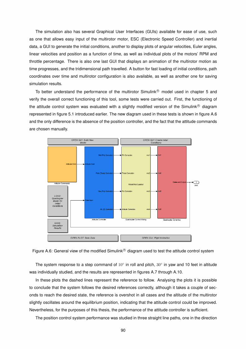
The simulation also has several Graphical User Interfaces (GUIs) available for ease of use, such
as one that allows easy input of the multirotor motor, ESC (Electronic Speed Controller) and inertial
data, a GUI to generate the initial conditions, another to display plots of angular velocities, Euler angles,
linear velocities and position as a function of time, as well as individual plots of the motors’ RPM and
throttle percentage. There is also one last GUI that displays an animation of the multirotor motion as
time progresses, and the tridimensional path travelled. A button for fast loading of initial conditions, path
coordinates over time and multirotor configuration is also available, as well as another one for saving
simulation results.
To better understand the performance of the multirotor Simulink R© model used in chapter 5 and
verify the overall correct functioning of this tool, some tests were carried out. First, the functioning of
the attitude control system was evaluated with a slightly modified version of the Simulink R© diagram
represented in figure 5.1 introduced earlier. The new diagram used in these tests is shown in figure A.6
and the only difference is the absence of the position controller, and the fact that the attitude commands
are chosen manually.
Figure A.6: General view of the modified Simulink R© diagram used to test the attitude control system
The system response to a step command of 10◦ in roll and pitch, 30◦ in yaw and 10 feet in altitude
was individually studied, and the results are represented in figures A.7 through A.10.
In these plots the dashed lines represent the reference to follow. Analysing the plots it is possible
to conclude that the system follows the desired references correctly, although it takes a couple of sec-
onds to reach the desired state, the reference is overshot in all cases and the altitude of the multirotor
slightly oscillates around the equilibrium position, indicating that the attitude control could be improved.
Nevertheless, for the purposes of this thesis, the performance of the attitude controller is sufficient.
The position control system performance was studied in three straight line paths, one in the direction
90

Figure A.7: Response of the system to a 10◦ step in roll
Figure A.8: Response of the system to a 10◦ step in pitch
of each axis, and the results are shown in figures A.11 through A.13.
These plots lead to the conclusion that the performance of the position controller is much worse than
that of the attitude controller. The pitch and roll should be approximately constant when the multirotor
moves in a straight line in the direction of the x and y axes respectively. Instead, the aircraft accelerates
too much, overshoots the reference position and is forced to brake by rotating in the opposite direction
than that of its motion, both when it reaches the reference velocity and when it reaches the reference
position. When moving up (in the direction of the z axis), there are no major issues other than a relatively
slow response. Despite the imperfections in control and the fact that for motion at constant velocity,
91

Figure A.9: Response of the system to a 30◦ step in yaw
Figure A.10: Response of the system to a 10 feet step in altitude
independently of its value, the motors angular velocity is not changed relative to the hover condition, as
discussed in chapter 5, this Simulink R© model of the multirotor was still used in the simulations due to
a lack of available alternatives. Therefore, the results obtained must be analysed with some criticism,
having the imperfections of the control system in mind.
92
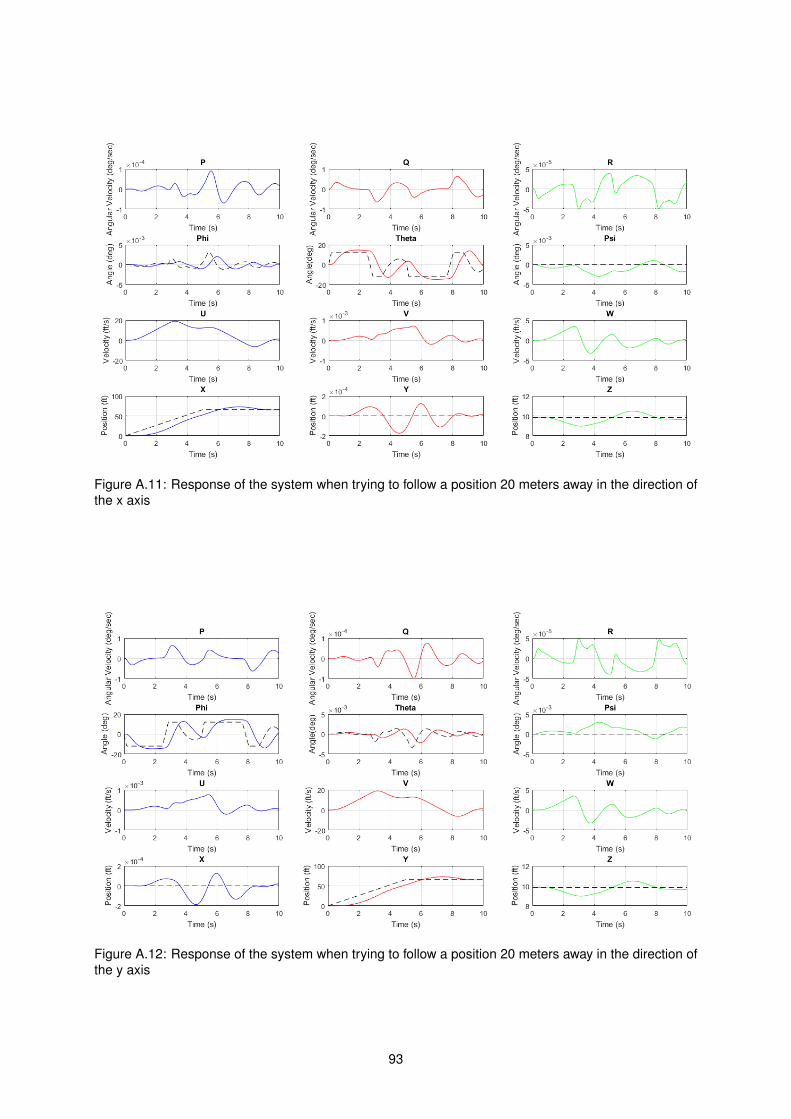
Figure A.11: Response of the system when trying to follow a position 20 meters away in the direction ofthe x axis
Figure A.12: Response of the system when trying to follow a position 20 meters away in the direction ofthe y axis
93

Figure A.13: Response of the system when trying to follow a position 10 meters away in the direction ofthe z axis
94