Energy Harvesting for Wireless Power Monitoring -

Implementing a Low Power, Low Data Rate Wireless

Network (OpenWSN)

David Stanislowski

Electrical Engineering and Computer SciencesUniversity of California at Berkeley

Technical Report No. UCB/EECS-2012-154

http://www.eecs.berkeley.edu/Pubs/TechRpts/2012/EECS-2012-154.html

June 2, 2012

Copyright © 2012, by the author(s).All rights reserved.

Permission to make digital or hard copies of all or part of this work forpersonal or classroom use is granted without fee provided that copies arenot made or distributed for profit or commercial advantage and that copiesbear this notice and the full citation on the first page. To copy otherwise, torepublish, to post on servers or to redistribute to lists, requires prior specificpermission.

Energy Harvesting for Wireless Power Monitoring

Implementing a Low Power, Low Data Rate Wireless Network (OpenWSN)David Stanislowski

M.Eng Candidate, Electrical Engineering and Computer Science Department, UC Berkeley

May, 2012

Group Members: Ameer Ellaboudy, Ankur Aggarwal, Ryan Moore, Vincent Lee

Advisers: Professors Bernhard Boser and Kristofer Pister

A combination of rising energy costs, a desire for national energy independence, and a

growing awareness of the dangers of global climate change is pushing Americans to do what

they can to save energy. Consumers now buy more fuel-efficient cars and appliances and are

growing more aware of their use habits. While it is easy to see how much gas your car uses,

beyond the labeling on major appliances at the point of sale, most consumers are unaware of how

much electricity these devices actually use. In this Masters of Engineering Capstone Project we

designed and implemented a wireless power monitor which sits on a conventional power outlet

and is thin enough that an appliance plugs throughs. The power of the appliance being plugged

through our device is monitored. The monitor is powered by either making direct contact with

the prongs of the plug or by inductively harvesting through a contactless transformer. The

latter case puts severe power restrictions on the mote which we overcame by using low-power

hardware and OpenWSN, a network stack intended for low power, low data-rate applications

such as ours.

Introduction

In the last fifty years, while household energy use has leveled off, energy prices have

increased continuously. In California, rates have gone from $0.11 to $0.15 per kilowatt-hour

from the year 2000 to 2010 [9]. There has also been a sustained growth in concern for global

climate change caused by human emissions of CO2, a large part of which is due to home and

office energy consumption. Efforts are being made at increasing efficiency -- for example in area

lighting, with development of fluorescent and LED lamps; and in appliances, with EnergyStar

ratings and the switch from linear to switching power supplies in so-called “wall-warts”

One problem which is preventing a lot of well-intentioned people from saving more

energy is that most people are simply unaware of where there is waste. It is not obvious when

a device is using more power than you think. They might only be warm to the touch. A typical

television set-top box consumes 20W while in standby mode [8]. If electricity costs $0.15/kWh,

that box costs about $26 per year just to be plugged in. This sort of vampire drain is difficult to

see from the utility bill yet the waste is significant.

Many companies have tried to address this lack of awareness already. P3 has been selling

its product, the Kill-a-Watt, for many years. The consumer plugs a product into the Kill-a-Watt

and it reports on an LCD screen how much power is being used. There are more sophisticated

products, like the Energy Hub, that wirelessly transmit data to a central hub with a screen or

internet connection where the data is analyzed and made available to the end-user. Yet none

of these products have reached ubiquity. There are two main reasons for this: The products

available today are fairly expensive ($30 per outlet for the Kill-a-Watt, $40 for EnergyHub) and

they are cumbersome to set up.

It is possible to overcome these issues and a big part will be to use a different kind

of wireless technology. Low power wireless networks have been in development since early

last decade -- IEEE802.15.4-2003, the original 15.4 standard, was released in 2003 -- and a

lot has changed since the first radios were sold and first network stacks were written. The

newest protocols -- IEEE802.15.4e-2012 was only published April 2012 -- are more robust

and lower power than those of ten years ago, yet none of the manufacturers we have found are

implementing them.

Fig 1. A diagram of our system setup

In this paper I will discuss the different types of low-power wireless network protocols. I

will then go over the challenges we had implementing OpenWSN and setting up the computing

hardware. Finally I will go over some suggestions for future work.

Potential Wireless Sensor Networking Protocols

In this section I will review existing wireless technologies suitable for wireless sensor

networks (WSNs).

Wifi (802.11)

The original 802.11 standard was released in 1997 for use in wireless local area networks

(WLANs). The first widely adopted standard was 802.11b, released in 1999. Subsequent releases

made improvements to bandwidth, range, and security. The target for this standard is computing,

PCs, smartphones, and other devices that send and receive a lot of data. The usage profile for

these devices is characterized by long idle periods unpredictably interspersed with periods of

potentially high traffic. Devices typically have either constant access to mains power or a sizable

rechargeable battery. [3]

The major downsides to the use of wifi in WSNs are the power requirements. As is

obvious from the development history, power efficiency is not the major focus, and in WSNs this

is key. Still, there have been attempts to adapt wifi to low-power applications. One such chipset

is the MicroChip MRF24WB0M which take 85mA to receive and 154mA to transmit data. It

also has a very low power hibernate mode but this will not save power if used for less than 30s.

[6]

Bluetooth (802.15.1)

Bluetooth was originally conceived in 1994 by private companies looking to replace

serial RS-232 interfaces. More recently it has come into wide use in a range of applications:

hands-free headsets for cell phones, low-rate data transfer between computers, video game

controllers, et cetera. Because of the portability of many of these devices, there was a concerted

effort to design the protocol to save power. [4]

More recently, the Bluetooth specification was updated to v4.0, also known as Bluetooth

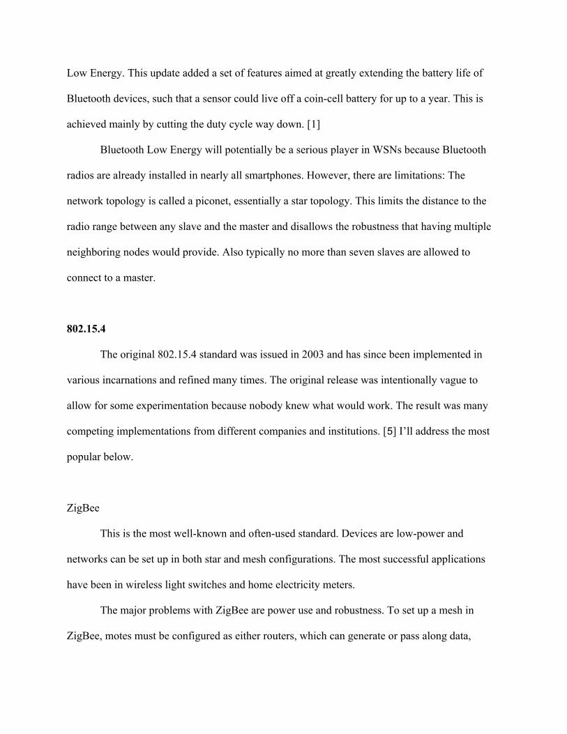
Low Energy. This update added a set of features aimed at greatly extending the battery life of

Bluetooth devices, such that a sensor could live off a coin-cell battery for up to a year. This is

achieved mainly by cutting the duty cycle way down. [1]

Bluetooth Low Energy will potentially be a serious player in WSNs because Bluetooth

radios are already installed in nearly all smartphones. However, there are limitations: The

network topology is called a piconet, essentially a star topology. This limits the distance to the

radio range between any slave and the master and disallows the robustness that having multiple

neighboring nodes would provide. Also typically no more than seven slaves are allowed to

connect to a master.

802.15.4

The original 802.15.4 standard was issued in 2003 and has since been implemented in

various incarnations and refined many times. The original release was intentionally vague to

allow for some experimentation because nobody knew what would work. The result was many

competing implementations from different companies and institutions. [5] I’ll address the most

popular below.

ZigBee

This is the most well-known and often-used standard. Devices are low-power and

networks can be set up in both star and mesh configurations. The most successful applications

have been in wireless light switches and home electricity meters.

The major problems with ZigBee are power use and robustness. To set up a mesh in

ZigBee, motes must be configured as either routers, which can generate or pass along data,

or leaf-nodes, which can only generate data. Routers must be on all the time to listen for

transmissions to be passed on. This necessitates a robust power supply. There is an option,

however, to run the network in “beacon” mode which will drop the duty cycle and save power.

Also, a ZigBee network is set up on a single channel. If it happens to choose a channel

where there is an interfering WiFi network or other RF noise source, there isn’t much that can be

done to fix it. [10]

WirelessHART

This protocol has seen major success in industrial applications. It was developed

specifically for industry with the involvement of many key companies. It implements TSCH

in all the nodes and is therefore low power and robust. Importantly for this market, it was

designed to allow interoperability between devices from different manufacturers, making it

attractive to businesses who might want to purchase different sensors from different vendors. But

unfortunately the WirelessHart standard is not made easily available for academic research. [2]

OpenWSN

The goal of the OpenWSN project is to “provide open-source implementations of a

complete protocol stack based on the to-be-finalized Internet of Things standards, on a variety

of software and hardware platforms.” The main work of the project is a network stack that

implements IEEE802.15.4 at 2.4 GHz in the physical layer, IEEE802.15.4E time-synchronized

channel hopping in the MAC layer, and RPL/UDP in the network layer. Because the project

includes a complete network implementation, is open-source, and is centered at UC Berkeley,

this is the protocol we decided to use.[7]

Challenges working with OpenWSN and GINA

The OpenWSN project has chosen a few different chipsets on which to focus its

development. The Guidance and Inertial Navigation Assistant (GINA) board is the one receiving

the most attention. GINA was designed to be used on small helicopters and therefore has a

microcontroller (MSP430), a radio (Atmel AT86), two accelerometers, a gyro, and a

magnetometer. For this project we only needed the microcontroller and radio. Implementing our

project on the GINA mote presented a few major challenges. In this section I discuss these issues.

Fig 2. GINA mote, top view, showing microcontroller (center chip with sticker attached) and radio (on right)

ADC Sample timing

In measuring power consumption of a device connected to mains power, it is necessary

to take measurements on alternating current lines. The signal must be sampled over at least

a full 60Hz wave which has a period 16.667ms. The duration of a sampling sequence should

be as close as possible to this period, and the closer it is, the less it matters where in the cycle

measurement begins -- the closer we get to 16.667ms, the more accurate our measurements

are. There is a timer implementation used with the current OpenWSN implementation called

OpenTimers. Any application running may create a timer which triggers either once or

periodically. OpenTimers keeps a list of all running timers and every time a timer fires, it runs

through the list to find the next timer trigger, which it then uses to set the next interrupt.

Fig 3. Possible sample timing. It does not matter when you start sampling so long as you are sampling exactly one period.

This would have been the simplest way to set up timing of the ADC, but unfortunately

we ran into a major issue. The timing of the ADC goes as follows: Every 1s, an application runs

to generate a single power reading. Each reading consists of a set of 16 samples taken at a rate of

1kHz. To take these samples, OpenTimers must fire every 1ms. Unfortunately, on the GINA this

is simply too much to process and the operating system overloads and crashes. This scheme was

tested on another more powerful microprocessor and in that case it worked fine, but changing

was not an option.

Fig 4. Sample and conversion timing of the ADC

The solution was to forget about OpenTimers and to use the hardware to time the ADC

so that it could be triggered once to read 16 samples. The MSP430 on the GINA mote has 16

memory registers available to the ADC. When the ADC is triggered, it fills its 16 registers which

can be read anytime before the next ADC reading. According to the user manual, the sample

time (tsample) may be set with a resolution of 4 cycles of the crystal oscillator (125us). Each

sample is followed by a 13 cycle long conversion. The best possible sample time should then be

34 cycles (34 cycles per sample with 16 samples is 17ms). This is achieved by setting the sample

and hold time to 4 cycles and the clock divider to 2 (sample time is 8 and convert time is 26

cycles).

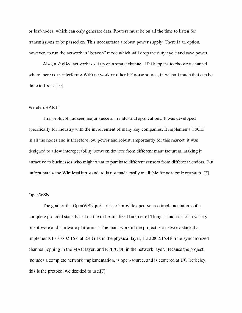
Fig 5. Example ADC measurements for 60Hz sine wave from function generator (left) and from our sensing circuit connected to a 60Hz light bulb (right). Each curve is a set of 16 measurements. You can

see that it is very close to a single cycle.

The data from the ADC is sent as-is in the packet payload. Because the packet is saved

as an array of bytes, each 12-bit reading is split across 2 bytes. The payload must therefore be at

least 32 bytes long and each pair is a single reading. Once the packet reaches its destination, the

DC offset must be removed (the offset is introduced in the circuitry because the ADC can only

handle 0-3V) and the RMS must be calculated to find the power.

Reducing Power Consumption of GINA

When we first began using GINA, measurements showed that it was consuming about

18mA of current during regular use. For our power harvesting application, this is too much. As it

turns out, the implementation of OpenWSN we started with was leaving on most unnecessary

components, such as the accelerometer. It also left the radio on all the time.

Turning off components is simple enough. Most of the components speak with the MSP

through the spi bus and have a command to shut off. One component can be turned off by

switching an I/O pin. The chips themselves may also be physically removed from the board,

saving even more power.

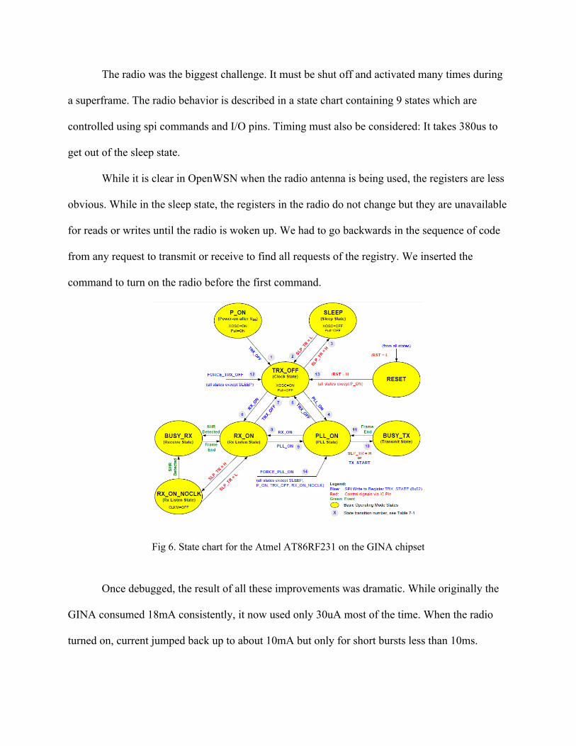
The radio was the biggest challenge. It must be shut off and activated many times during

a superframe. The radio behavior is described in a state chart containing 9 states which are

controlled using spi commands and I/O pins. Timing must also be considered: It takes 380us to

get out of the sleep state.

While it is clear in OpenWSN when the radio antenna is being used, the registers are less

obvious. While in the sleep state, the registers in the radio do not change but they are unavailable

for reads or writes until the radio is woken up. We had to go backwards in the sequence of code

from any request to transmit or receive to find all requests of the registry. We inserted the

command to turn on the radio before the first command.

Fig 6. State chart for the Atmel AT86RF231 on the GINA chipset

Once debugged, the result of all these improvements was dramatic. While originally the

GINA consumed 18mA consistently, it now used only 30uA most of the time. When the radio

turned on, current jumped back up to about 10mA but only for short bursts less than 10ms.

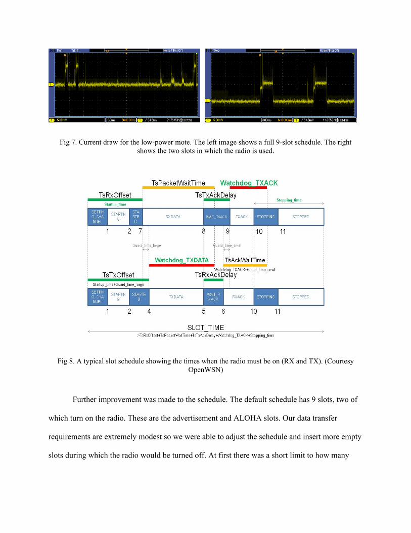
Fig 7. Current draw for the low-power mote. The left image shows a full 9-slot schedule. The right shows the two slots in which the radio is used.

Fig 8. A typical slot schedule showing the times when the radio must be on (RX and TX). (Courtesy OpenWSN)

Further improvement was made to the schedule. The default schedule has 9 slots, two of

which turn on the radio. These are the advertisement and ALOHA slots. Our data transfer

requirements are extremely modest so we were able to adjust the schedule and insert more empty

slots during which the radio would be turned off. At first there was a short limit to how many

slots could be fit because of how the schedule was saved. Each slot was represented by a

memory hungry object in an array as long as the number of slots in the superframe. This was

later fixed by implementing a linked list so that empty slots could be inserted with little cost to

memory.

Slots per Frame Average Current

9 660uA

20 320uA

100 100uA

200 68uA

Table 1. Current draw depending on the choice of superframe length

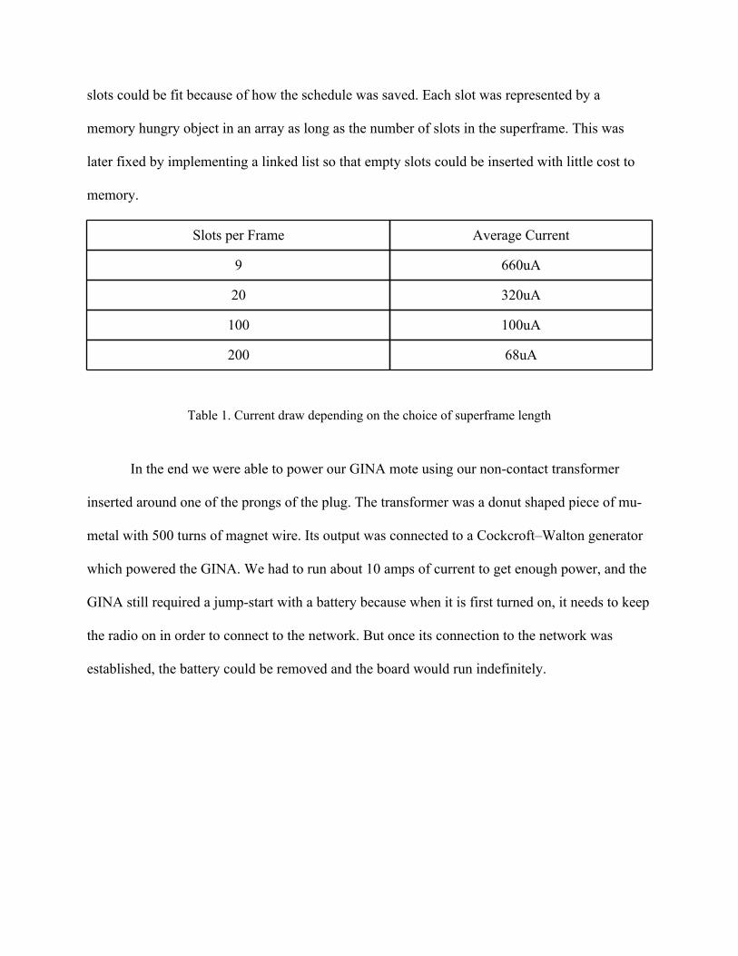
In the end we were able to power our GINA mote using our non-contact transformer

inserted around one of the prongs of the plug. The transformer was a donut shaped piece of mu-

metal with 500 turns of magnet wire. Its output was connected to a Cockcroft–Walton generator

which powered the GINA. We had to run about 10 amps of current to get enough power, and the

GINA still required a jump-start with a battery because when it is first turned on, it needs to keep

the radio on in order to connect to the network. But once its connection to the network was

established, the battery could be removed and the board would run indefinitely.

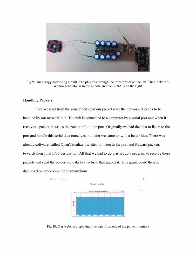
Fig 9. Our energy harvesting circuit. The plug fits through the transformer on the left. The Cockcroft-Walton generator is in the middle and the GINA is on the right.

Handling Packets

Once we read from the sensor and send our packet over the network, it needs to be

handled by our network hub. The hub is connected to a computer by a serial port and when it

receives a packet, it writes the packet info to the port. Originally we had the idea to listen to the

port and handle this serial data ourselves, but later we came up with a better idea. There was

already software, called OpenVisualizer, written to listen to the port and forward packets

towards their final IPv6 destination. All that we had to do was set up a program to receive these

packets and send the power use data to a website that graphs it. This graph could then be

displayed on any computer or smartphone.

Fig 10. Our website displaying live data from one of the power monitors

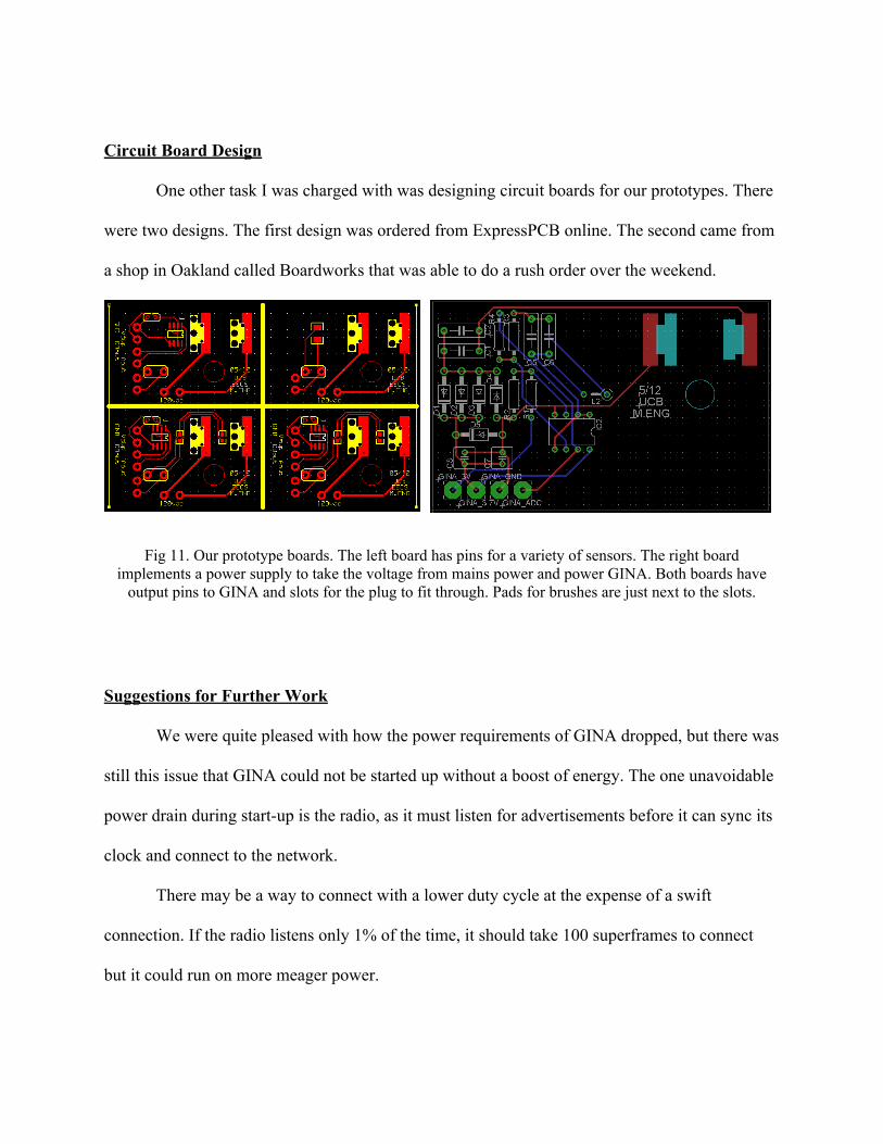
Circuit Board Design

One other task I was charged with was designing circuit boards for our prototypes. There

were two designs. The first design was ordered from ExpressPCB online. The second came from

a shop in Oakland called Boardworks that was able to do a rush order over the weekend.

Fig 11. Our prototype boards. The left board has pins for a variety of sensors. The right board implements a power supply to take the voltage from mains power and power GINA. Both boards have

output pins to GINA and slots for the plug to fit through. Pads for brushes are just next to the slots.

Suggestions for Further Work

We were quite pleased with how the power requirements of GINA dropped, but there was

still this issue that GINA could not be started up without a boost of energy. The one unavoidable

power drain during start-up is the radio, as it must listen for advertisements before it can sync its

clock and connect to the network.

There may be a way to connect with a lower duty cycle at the expense of a swift

connection. If the radio listens only 1% of the time, it should take 100 superframes to connect

but it could run on more meager power.

In forwarding our packets to the website, there were many unnecessary steps. The path

went as follows: GINA hub to OpenVisualizer to LBR (a server running off-site) to another

laptop running a python script and finally to the website to display data. OpenVisualizer could be

altered to send packets directly to that website.

For a proof of concept, these issues were not terribly significant, but if this design is to be

developed further, the above issues should be addressed.

Conclusion

In conclusion, we designed and built devices to monitor electrical plug level power use.

These devices fit in between the plug and the wall and were powered either by directly

contacting the prongs of the plug or by inductive coupling to the current flow through one of the

prongs. We set up a network protocol called OpenWSN to connect two leaf nodes to a hub and

were able to measure the power being used, send that data as a packet over our network and then

into the internet where it finally reached a website that plotted the data with a delay on the order

of a few seconds.

Fig 12. Our contact plug-through power monitor. A plug fits through the holes on the top right.

Acknowledgements

I would like to thank Fabian Chraim and Xavier Vilajosana for the many hours they spent

teaching me how to program GINA and fix whatever bugs I encountered; Branko Kerkez for

helping me handle data from the sink to the internet; and Thomas Watteyne and the rest of the

OpenWSN team for offering me help whenever I went to their meetings.

Citations

[1] “BLUETOOTH SPECIFICATION Version 4.0”. Bluetooth Special Interest Group. https://

www.bluetooth.org/Technical/Specifications/adopted.htm.

[2] “HART Communication Protocol - WirelessHART Technology,” accessed April 14, 2012, http://

www.hartcomm.org/protocol/wihart/wireless_technology.html.

[3] “IEEE 802.11: Wireless LAN Medium Access Control (MAC) and Physical Layer (PHY)

Specifications,” (2007 revision). IEEE-SA. 12 June 2007.

[4] "IEEE Std 802.15.1-2005 – IEEE Standard for Information technology – Telecommunications and

information exchange between systems – Local and metropolitan area networks – Specific

requirements Part 15.1: Wireless Medium Access Control (MAC) and Physical Layer (PHY)

Specifications for Wireless Personal Area Networks (WPANs)," IEEE Computer Society, New

York, NY, 14 June 2005.

[5] “IEEE Std 802.15.4-2006 -- Wireless Medium Access Control (MAC) and Physical Layer (PHY)

Specifications for Low-Rate Wireless Personal Area Networks (WPANs),” IEEE Computer

Society, New York, NY, 8 September 2006.

[6] MicroChip, MRF24WB0MA/MRF24WB0MB Data Sheet (USA: Microchip Technology Incorporated,

2010 - 2011).

[7] “OpenWSN,” accessed March 16, 2012, http://openwsn.berkeley.edu/.

[8] “Standby Power,” accessed March 16, 2012, http://standby.lbl.gov/data.html.

[9] “State Electricity Profiles 2010,” US Energy Information Administration, Washington, DC, 27

January 2012.

[10] “ZigBee Specification,” (revision 17). Zigbee Standards Organization. 17 January 2008.

Appendix - Example Code Setting up the ADC: // SHT0_0 and SHT1_0: Sample-and-hold time is 4 ADC12CLK cycles // MSC: Multiple sample and conversion: sample-and-conversions

performed automatically // ADC12ON: ADC12 on ADC12CTL0 = SHT0_0 + SHT1_0 + MSC + ADC12ON; // CSTARTADD_0: Conversion start address is 0 // SHP: Sample-and-hold pulse-mode select, sourced from the sampling

timer // CONSEQ_1: Conversion sequence mode select, Sequence-of-channels // ADC12SSEL_1: ADC Clock Source (32kHz crystal, 31.25us) // ADC12DIV_1: ADC Clock Divider is 2 ADC12CTL1 = CSTARTADD_0 + SHP + CONSEQ_1 + ADC12SSEL_1 + ADC12DIV_1; ADC12MCTL0 = INCH_0; // ADC12MCTL0 <- P6.0 = open ADC ADC12MCTL1 = INCH_0; ADC12MCTL2 = INCH_0; ADC12MCTL3 = INCH_0; ADC12MCTL4 = INCH_0; ADC12MCTL5 = INCH_0; ADC12MCTL6 = INCH_0; ADC12MCTL7 = INCH_0; ADC12MCTL8 = INCH_0; ADC12MCTL9 = INCH_0; ADC12MCTL10 = INCH_0; ADC12MCTL11 = INCH_0; ADC12MCTL12 = INCH_0; ADC12MCTL13 = INCH_0; ADC12MCTL14 = INCH_0; ADC12MCTL15 = INCH_0 + EOS; // End of Sequence Writing to the packet: for (i=0;i<N_SAMPLES;i++) { pkt->payload[2*i] = (adc_samples[i]>>8)&0xff; pkt->payload[2*i+1] = (adc_samples[i]>>0)&0xff; } Turning off unnecessary components: //first initialize them gyro_init(); large_range_accel_init(); magnetometer_init(); //sensitive_accel_temperature_init(); //Does not need init //then turn them off gyro_disable();

large_range_accel_disable(); magnetometer_disable(); sensitive_accel_temperature_disable(); radio_rfOff(); // Initialized elsewhere Turning on the radio:void radio_rfOn() { if (radio_vars.state == RADIOSTATE_RFOFF) { PORT_PIN_RADIO_SLP_TR_CNTL_LOW(); //SLP_TR = L, end radio sleep while((radio_spiReadReg(RG_TRX_STATUS) & 0x1F) != TRX_OFF); //

Wait for awake }} Turning off the radio:void radio_rfOff() { int reg = (radio_spiReadReg(RG_TRX_STATUS) & 0x1F); if ((radio_vars.state != RADIOSTATE_RFOFF) && (reg != SLEEP) &&

(reg != P_ON)) { radio_vars.state = RADIOSTATE_TURNING_OFF; radio_spiReadReg(RG_TRX_STATUS); // turn radio off radio_spiWriteReg(RG_TRX_STATE, CMD_FORCE_TRX_OFF); while((radio_spiReadReg(RG_TRX_STATUS) & 0x1F) != TRX_OFF); //

busy wait until done PORT_PIN_RADIO_SLP_TR_CNTL_HIGH(); //SLP_TR = H, radio sleep, In

SLEEP state register not accessible leds_radio_off(); // change state radio_vars.state = RADIOSTATE_RFOFF; }}