1

Scriptum of the course No. 351-0510-00

Energy Economics and Policy

(Energiewirtschaft und Energiepolitik)

SS 2007

24 May 2007

Prof. Dr.-Ing. Eberhard Jochem

Chair of economics and energy economics Lehrstuhl für Nationalökonomie und Energiewirtschaft

2

Content Date Page (Übersicht zur Vorlesung) 3

Recommended books, monographs, statistics, and publications 7

I) Energy resources, sustainability, energy statistics

• Reserves and resources of non-renewable energies 22.3. 13

• Energy statistics 29.3. 24

• Ecological economics, sustainability concept 29.3. 31

• The concept of sustainable development 5.4. 38

II) Drivers of energy demand

• Energy flow diagram, starting at the energy services 12.4. 43

• Exercise/ Übung 1 discussion and solutions 12.4.

• Energy efficiency potentials and energy intensities 19.4. 45

• Private households, services, industry, transportation, prices 26.4.

• Cost of energy conversion and end-energy uses, external cost 3.5.

III) Energy economic analysis and projections

• Scenario technique, modelling, and boundary conditions 10.5. 60

• Development of energy demand by different types of models-

advantages and limitations of different types of models 24.5.

IV) Obstacles and market imperfections and related portfolios of energy- and climate policy

• Obstacles of energy efficiency and substitution 31.5.

• Market imperfections and policy instruments I 7.6.

• Energy and climate policy II and their evaluation 14.6.

V) Annex

• Glossary 32

You will find additional information for the course and the exercises at

http://www.cepe.ethz.ch/education/EnergyEconomicsCepe

3

Energy economics and policy (SS 2007)

Prof. Dr.-Ing. Eberhard Jochem Course: Thursdays, 15-17 h, room: ML H44

Start: March 22, 15.15 h, room: ML H44

Objectives:

The students are introduced to basic knowledge of resource and energy economics, to renewable and non-renewable energies, energy statistics, energy markets, energy efficiency potentials, obstacles and market imperfections and related energy policies.

The methods covered are cost estimation of new energy technologies, scenario technique, energy models (bottom up and top down), and external cost of energy use. The energy policy section covers general and specific policy instruments and also includes climate change policy, related instruments and their implementation.

In general, the students mostly educated in natural sciences and engineering have the opportunity to develop their "coupling competence" to concepts of economics and policy and to use this knowledge in their professional life in interdisciplinary working teams. There are two chances to deepen the knowledge of the course: three exer-cises and a written paper (of about 10 to 12 pages) related to issues of energy eco-nomics and policy.

Overview of the course: Energy Economics and Policy (Energiewirtschaft und Energiepolitik)

No. date Topic/Thema lecturer Bibliography

Introduction and energy resources and energy statistics

1

22.3.

Energy as natural resource • economics of natural resources • reserves & resources of energy

Wickart/ Jochem

K. Blok 2006, Chapt. 4 Spreng, 1995, Kap. 1 BFE and IEA/OECD

2

29.4. Energy statistics (descriptive) • Definitions, units, conversion fac-

tors • Energy balances (specially Swit-

zerland) • cumulative energy demand

Energy and sustainability • ecological economics

Jochem www.admin.ch/bfe/ http://www.iea.org/ www.worldenergy.org K. Blok 2006, Chapt. 2 K. Blok 2006, Chapt. 6

CEPE / D-MTEC ETH Zentrum ZUE E 8 CH-8092 Zürich Tel. +41-44632 06 50 Fax +41-44-632 10 50 http://www.cepe.ethz.ch

4

• Brundlandt-Commission; • sustainability concepts

3 5.4. Drivers of energy demand • Energy flow diagrams of indus-

trialised countries & world • Energy services and intensities • climate change and environ-

mental pollution

Jochem K. Blok, 2006, Chapt. 2

4 12.4. Exercise 1 discussion and so-lutions

M. Jakob Literature of the first three courses

Energy demand and conversion - Drivers, sectors, and cost

5 19.4. Energy chains and efficiency • Energy services, useful energy,

final energy with respect to space heat, service sector, in-dustry

• Energy efficiency potentials, theoretical, technical, welfare-economic, macro and micro-economic, expected

• The 2000 Watt/cap society

Jochem K. Blok 2006, Chapt. 10 Hensing, Pfaffenberger, Ströbele 1998, Goldemberg, J. 2000; Kap. 6; Romm, J.J. 1999: Cool Com-panies Geiger, B. u.a., 1999 Jochem et al. 2003

6 26.4. Energy services and demand (Perspectives of the BFE) • private households • service and industrial sector • transport sector • conversion sector • structural change

Jochem K. Blok 2006, Chapt. 3 BFE 2007, Synthesis Report Diekmann, J. u.a. 1999,

7 3.5. Cost of energy conversion and end-use technologies) • technologies in cost competition • cost reduction by learning and

economies of scale • cost optimal mix of energy con-

version technologies

Jochem K. Blok 2006, Chapt. 11 Hensing, Pfaffenberger, Ströbe-le 1998, Kap. 11 Hirschberg, Jakob 1999

7 3.5. External cost and their inter-nalisation • external effects (environment,

resources) • Identification, quantification,

monetarisation • external cost in energy conver-

sion and use

Jochem Stiglitz, J. 2000, Kap. 8 Pindyck, Rubinfeld 1998, Kap. 18 Pearce und Turner 1990, Kap. 4-6

5

Energy economic analysis and projections

8 10.5. Scenario techniques and boundary conditions • Methodology of Scenario design • examples of the energy perspec-

tives Energy modelling • macro economic energy models • process-oriented energy models • linking TD und BU models (hy-

brid models)

Jochem Energy perspectives, BFE, 2007 K. Blok 2006, Chapt. 14 Jochem/Jakob, 2003 Hensing, Pfaffenberger, Ströbele 1998, Chap..11 Heinloth, K. 1998, K. Blok 2006, Chapt. 14 Goldemberg, J. 2000, Kap.6 Jochem, Kuntze, Patel 2000

9 24.5. Energy demand projections and limitations of methods • macro models (technology pro-

gress, closed causal relation-ships)

• Simulation und Optimising of bot-tom up (BU) models (techn. pro-gress, partial analyses)

• combination of model types by Integration (soft and hard links)

Jochem K. Blok 2006, Chapt. 14 Hensing, Pfaffenberger, Ströbele 1998, Kap. 11 K. Blok, 2006 Chapt. 14 Heinloth, K. 1997, Kap. 1 und 14 Bartzsch, W.H. 1997

Obstacles, market imperfections, opportunities, and energy and climate policy

10 31.5. Obstacles of energy efficiency and substitution • company internal problems and

situations • Preferences, prestige, psycho-

logical aspects • legal and other unfavourable

boundary conditions

Aebi-scher

Sorrell et al. 2004, Chapt. 2-5 Jochem, 2004; Ostertag u.a. 2000 Jochem, Kuntze, Patel 2000

11 7.6. Market imperfections • Market power, the role of media • external effects of technological

options • international issues (competi-

tiveness)

Energy policy instruments I • general instruments • international co-ordination (EU,

G8, OECD, Kyoto)

Jochem Sorrell et al. 2006, Chapt. 2-5 Ostertag 2003 Jochem, Kuntze, Patel 2000Ziesing u.a. 1997 Hensing, Pfaffenberger, Ströbe-le 1998, Chapt.. 13 – 15 Sorrell et al. 2004 Chapt. 7 + 8 K. Blok 2006, Chapt. 15

12 14.6. Energy policy instruments II • sector- und technology specific

policy measures

Jochem

Sorrell et al. 2006 Chapt 7 and 8 K. Blok 2006, Chapt. 15

6

• Policy portfolios as reaction on simultaneous obstacles

• International trade

Evaluation of energy and climate policies • evaluation criteria • direct and indirect effects • policies of innovation • long term effects (discounting?)

Ziesing u.a. 1997 Hensing, Pfaffenberger, Ströbele 1998, Kap. 13 – 15 Sorrell et al. 2006 Chapt 7 and 8 K. Blok 2006, Chapt. 15 Hensing, Pfaffenberger, Ströbe-le 1998, Kap. 13 – 15

13 21.6 Conclusions of the course discussion of exercise No.3

Jochem, Wickart

Sorrell et al. 2006 Blok 2006 Manuscript Jochem

exam

5.7.

Semester end exam (eventu-ally, some who leave earlier have to pass an oral exam)

Jochem, Wickart

no manuscript allowed, only small calculator accepted

Important Information (Mitteilungen) for Testate and exams

Testate conditions for the Testate:

• for all students to receive 3 credits: active participation at the courses, passing 2 exercises out of 3 minimum, and passing the exam

exams Students who want to pass a Semester-Endprüfung : the written 90 minutes lasting exam takes place at July 5, 2007 between 15.15-16.45 h Confirmation per Email the latest until one day before the examination day at: mwickart@ethz.ch, 044 632 03 98.

Exercises/ Übun-gen

The course has two hours per week and three exercises. The exercises have to be made within two weeks after distribution. The results of the exercises will be explained in some of the second hour of the course. The solutions will be simultaneously published at the homepage of CEPE (http://www.cepe.ethz.ch/education/EnergyEconomicsCepe). Specific hours for exercises are not planned.

You may ask the following assis-tents

Sprechstunde via oral or e-mail confirmation: Andrea Honegger Tel.-No.: 044 632 05 76 (course and exercises: Prof. Jochem) ahonegger@ethz.ch Marcel Wickart Tel.-No.: 044 632 03 98 (Economic aspects) mwickart@ethz.ch Bernard Aebischer Tel.-No.: 044 632 41 95 (technical and policy aspects) baebischer@ethz.ch

7

8

Recommended books, monographs, statistics, and publications Recommended books and monographs Banks F.E. (2000). Energy Economics: A Modern Introduction, Kluwer Academic Publishers,

Dordrecht

Blok K. (2006). Introduction to Energy Analysis, Techne Press, Amsterdam, the Netherlands

Hensing I., W. Pfaffenberger und W. Ströbele (1998). Energiewirtschaft – Einführung in Theo-rie und Politik, Oldenbourg, München, Germany

Griffin J.M. und H.B. Steele (1986), Energy Economics and Policy, Academic Press, Orlando

Sorrell S., O’Malley E., Schleich, J. and Scott, S. (2004). The Economics of Energy Efficiency – Barriers to Cost-Effective Investment, Edward Elgar Publishing Limited, Cheltenham, UK

Important energy statistics BFE, Bundesamt für Energie, (several years). Schweizerische Gesamtenergiestatistik 2005.

Bern ; http://www.bfe.admin.ch/themen/00526/00541/00542/00631/index.html?lang=de

BFE Bundesamt für Energie, (several years). Schweizerische Elektrizitätsstatistik, 2005. Bern 2006. http://www.bfe.admin.ch/themen/00526/00541/00542/00630/index.html?lang=de

IEA/OECD, (several years) Energy Balances for OECD-countries. Paris 2001; www.iea.org/stat.htm

World Energy Council (WEC). (several years) Country statistics and survey on energy re-sources. http://www.worldenergy.org/wec-geis/edc/default.asp

Publications to individual issues of the course Baron, R., Jochem, E. Kristof, K. (2005): Studie zur Konzeption eines Programms für die

Steigerung der Materialeffizienz in mittelständischen Unternehmen. Arthur D. Little, Fh-Inst. f. System- und Innovationsforschung, Wuppertal-Institut, Wiesbaden/Karlsruhe/-Wuppertal

Bartzsch, W.H. (1997), Betriebswirtschaftslehre für Ingenieure.

Bonomo, S., M. Filippini und P. Zweifel (1998), “Neue Aufschlüsse über die Elektrizitäts-nachfrage der schweizerischen Haushalte”, Schweiz. Zeitschrift für Volkswirtschaft und Statistik, Vol.134 (3), S. 415-436.

Commission of the European Communities (2006) Action Plan for Energy Efficiency: Realis-ing the Potential COM(2006)545 final, October 19, Brussels

Cuhls, K., Blind, K., Grupp., H. (1998), Delphi '98 Umfrage. Studie zur globalen Entwicklung von Wissenschaft und Technik. Methoden- und Datenband. Fh-ISI im Auftrag des BMBF, Karlsruhe, Februar 1998

Diekmann, J. u.a. (1999), Energie-Effizienz-Indikatoren. Umwelt und Ökonomie 32 Physika Heidelberg

Filippini, M. (1997), Elements of the Swiss Market for Electricity. Physica-Verlag, Berlin.

Geiger. B., E. Gruber, W. Megele (1999), Energieverbrauch und Einsparung in Gewerbe, Handel und Dienstleistung. Physika Heidelberg

Goldemberg, Jose (2000), World Energy Assessment. UNDP New York , Kap. 6 End-use efficiency

9

Heinloth, Klaus, (1997), Die Energiefrage – Bedarf und Potentiale, Nutzung, Risiken und Kos-ten. Vieweg, Braunschweig.

Hirschberg, S. und M. Jakob (1999), Cost Structure of the Swiss Electricity Generation under Consideration of External Costs, SAEE Seminar Strompreise zwischen Markt und Kos-ten: Führt der freie Strommarkt zur Kostenwahrheit?, Bern.

Hunt, S. und G. Shuttleworth (1996), Competition and Choice in Electricity, Wiley, Chichester

IEA (International Energy Agency) (2006): Energy Technology Perspectives 2006 – Scenarios and Strategies – in support of the G8 Plan of Action. OECD, Paris

IPCC (Intergovernmental Panel on Climate Change) (2001): Climate Change 2001 - Mitiga-tion: Contribution of Working Group III to TAR. Cambridge Univ. Press, Cambridge UK

Jochem, E., U. Kuntze, M. Patel (2000), Economic Effects of Climate Change Policy - Under-standing and Emphasizing the Costs and Benefits. ISI Karlsruhe

Jochem, E., Jakob, M. (2003), Energieperspektiven und CO2-Reduktionspotenziale in der Schweiz bis 2010, vdf-Verlag, ISBN 3-7281-2916-X.

Jochem, E. (edr) (2004), Steps towards a sustainable development - A White Book for R&D of energy-efficient technologies, ISBN 3-9522705-0-4.

Jochem, E. (2007): Using Energy and Materials More Efficiently – Large and Profitable Poten-tials, But Little Attention from Energy and Climate Policy. Die Energiepolitik zwischen Wettbewerbsfähigkeit, Versorgungssicherheit und Nachhaltigkeit Vierteljahreshefte zur Wirtschaftsforschung 76(2007)1, p.50-62

Keating, M. (1995), Agenda for Change, Centre for Our Common Future, Geneva (ex. auch auf Deutsch)

Markewitz, P. u.a. (1998), Modelle für die Analyse energiebedingter Klimagasreduktions-Strategien. Reihe Umwelt, Forschungszentrum Jülich

OECD/IEA (2005), Resources to Reserves – Oil & Gas Technologies for the Energy Markets of the Future, International Energy Agency (IEA), Paris.

Ostertag, K. (2003): No-Regret Potentials in Energy Conservation – An Analysis of Their Relevance, Size, and Determinants. Physica , Heidelberg

Pearce, D.W. und R.K. Turner (1990), Economics of natural resources and the environment, Harvester Wheatsheaf, New York, Kapitel 4-6

Pindyck, S.R. und D.L. Rubinfeld (1998), Mikroökonomie, 4. Auflage, München: Oldenbourg.

Romm, J. J. (1999), Cool companies - How the Best Businesses Boost Profits and Productiv-ity by Cutting Greenhouse Gas Emissions. Earthscan, London.

Samuelson, P.A. und W.D. Nordhaus (1998), Volkswirtschaftslehre, Ueberreuter, Anhang 5 und 7.

Spreng D. (1995), Graue Energie, vdf-Hochschulverlag an der ETH Zürich

Spreng D. und J. Schwarz (1993), Energie – ihre Bedeutung für die Wirtschaft, Bundesamt für Konjunkturfragen, EDMZ Bern, Bestellnummer: 724.316 d

Stiglitz J.E. (2000), Economics of the Public Sector, W. W. Norton, New York

Rahmeyer F. (1999), Preisbildung im natürlichen Monopol, WiST Heft 2, Februar 1999, S.69-75.

VDI-Gesellschaft für Energietechnik (2000), Energie und nachhaltige Entwicklung, VDI/GET Düsseldorf

Viscusi W. K., Vernon, J. M. und Harrington, J. (1995), Economics of regulations and antitrust, second edition, MIT Press, Chapt 11.

Ziesing H.-J. et al. (1997), Szenarien und Massnahmen zur Minderung von CO2-Emissionen in Deutschland. in: Politikszenarien für den Klimaschutz. Band 1 (Stein und Strobel Hrsg.) Reihe Umwelt Forschungszentrum Jülich.

10

Overview and short introduction

The core competence of the students participating in this course is in the fields of natural and environmental sciences, engineering, construction, or architecture. The objective of the course is to develop "coupling competence" of neighbouring disci-plines, methods and data, relevant for energy economics and energy policy analysis (see Figure 0-1). Energy economics and policy is a quite interdisciplinary field of sci-entific analysis and basic knowledge in energy technology, thermodynamics, and micro economics is a prerequisite to fully benefit from the course.

Energy statistics

- descriptive- analytical- Data sourcesEnergy resources

- Reserves- Resources

Eficient use of energy

- Potentials of efficiency- Energy services

Energy policy- Measures and portfolios

- national, Canton level- EU und international

Obstacles andMarket imperfections

- company internal obstacles - general deficits- sectoral obstacles

Energy projections

- Scenario technique- Modelling

Markets and externalities- Production cost and prices- External cost

Energy demand- drivers, - specific demand

Engineering

Construction

EnvironmentalSciences

Physics

Energy statistics

- descriptive- analytical- Data sourcesEnergy resources

- Reserves- Resources

Eficient use of energy

- Potentials of efficiency- Energy services

Energy policy- Measures and portfolios

- national, Canton level- EU und international

Obstacles andMarket imperfections

- company internal obstacles - general deficits- sectoral obstacles

Energy projections

- Scenario technique- Modelling

Markets and externalities- Production cost and prices- External cost

Energy demand- drivers, - specific demand

Engineering

Construction

EnvironmentalSciences

Physics

Figure 0-1: Overview over the course on "Energy Economics and Policy" – devel-oping coupling competence to other disciplines, methods and statistics

Energy use is labelled as the "blood" of industrialised countries to stress the impor-tance of a simple mean that allows societies to live in great comfort and safety. How-ever, the easy and inexpensive availability is increasing at stake because of three challenges: (1) a foreseeable tenfold increase of global gross domestic product which could induce at least a fivefold increase in primary energy demand, (2) the expected energy price increases due to the maximum production of oil within the next decades, and (3) the climate change mainly due to the 80% fossil fuel use of primary energy at present. The course will cover the analysis and possible solutions of these chal-lenges by pointing to methods of analysis, potential solutions, their obstacles and optional policies.

11

At what level of economics we are talking about? There are different levels of economics and the same expression (such as cost or benefit) may not mean the same at those different levels. This fact leads to many misunderstandings in discussions and readings in journals. The course distinguishes four levels of economics, which is important to keep in mind (see Figure 0-2):

• the level of business economics and project evaluation (see Chapt. 5),

• the sectoral (micro) economic level such as the energy supply sector (Chapt. 6, 9)

• the macro economic level (see Chapt. 8, 9), and

• the welfare economics level (including external costs and benefits not in-cluded in market prices of products and services; see Chapt. 11)

The course covers these four levels and refers to the different types of quantitative models. The course also refers to typical models that are being used at the different levels of economic evaluation; and there are types of models that build a bridge be-tween the different levels; e.g., the input/output model is a very convenient and pow-erful model type building a bridge between the process-oriented bottom up models and the macro economic models; the latter also can handle externalities in principle (see Figure 0-2).

Key issues : technological change, shifts in energy supply, energy-economy interactions, energy-

environment interactions and energy-society interactions

external effects(external costsand benefits)

economics(economy-wide and

macro effects)

energy system assessment(supply and demand,

technology)

business economics(project evaluation)

Micro :Sector level

« micro-micro » :Technology and site

level

Macro :National/regional

level

bottom-up, technology-

oriented

top-down, sector-

oriented

Types ofmodels:

I/O-models

Level ofeconomics :

Figure 0-2: Overview of different levels of economic analysis

However, this course can only give an overview on aspects of energy technologies, on energy models, obstacles, motivations, market imperfections, and policies. There are additional courses on these issues at ETH, but this course tries to give a holistic view how all the elements of technology innovation and potentials, of economics and

12

behavioural sciences as well as policy sciences work together – a gigantic causal relationship of a part of a society.

13

I. Resources of energy, sustainable development, and energy statistics

Energy as a natural resource and its role in the economy and society

Objectives:

The understanding of natural resources and the state of the art of statistics are the objectives of this section of the course. The student should be able to distinguish different types of reserves and resources and understand the reserve to production ratio, stationary and dynamic, the theory of natural economics (back stop technology, Hotelling rule) and the national energy statistics (energy flow diagram), the cumula-tive energy demand and some understanding of the role of energy in industrialised countries. Finally, the basic principle of sustainable development (in its hard and soft interpretation) should be known.

I.1. Reserves and resources of non-renewable energies

If sustainability demands that “present generations should use non-renewable re-sources without compromising the capacity of future generation to satisfy their own needs”, two questions arise regarding fossil fuels:

• What are the theoretically maximum quantities of fossil fuels mankind could use in the future? How long will they last, giving constant or even increasing use in the future decades?

• What are the alternatives of fossil fuels? Can they be developed early enough and at similar cost and prices as the cost level of fossil fuel is today?

Global primary energy demand can be distinguished in several phases (see Figure I.1-1): (1) a long period over eight decades with slowly increasing demand (1.7 % per year) until the end of World War II which resulted in an increase by a factor of 4 be-tween 1875 and 1950. (2) A steep increase (by 4.7 % per year) and also in per capita energy use between 1950 and 1979; (3) still an increase in global energy demand, but not faster than the growth of world population, which means a stagnation per cap-ita primary energy use thereafter (see Figure I.1-1).

For the uninformed reader this may be frightening as only 15 % of world population (about 1 Bill. people) are living in the comfortable level of an industrialised country, and there may be another 8 Bill people who will want to live as comfortable as the industrialised world does. This would mean a tenfold increase of global gross domes-tic product at the end of this century compared to today and again a fourfold increase of primary energy demand where an improvement of energy productivity of 1 % per year has been already considered.

However, there is some indication that the increase in primary energy demand will slow down; the per capita world primary energy demand stabilised during the last 25 to 30 years around 70 GJ/cap and year (see Figure I.1-1). The reason is higher effi-ciency gains as the usual 1 % per in OECD countries and a substantial energy effi-

14

ciency improvement in former centrally planed economies where waste of energy (being a public good) was extremely high compared to Western levels.

The experience of the two oil price crises in 1973 and 1979/80 (see Figure I.1-2) showed a substantial reaction of markets, technology producers, and policy making leading to more efficient use of energy and energy substitution towards natural gas, nuclear power and renewable energies. Awareness has grown that fossil fuel re-sources are not abundant, but need constant exploration efforts and improvement of the production technologies, but also alternative energy sources in the longer term.

Nuclear powerNatural gas

Lignite

Oil

Hard coal

Wood

Figure I.1-1 World primary energy demand, per capita energy use, and world population, 1875 to 2000

The so called "oil crisis" of 1973 already has changed the structure of primary energy use of the world: whereas in 1973, oil use accounted for 45 % of total primary energy use, 27 years later the share of oil has dropped to 34.9 % (see Figure I.1-3) and tends to achieve 33 % within this decade. Natural gas and nuclear energy grew dur-ing this period by five percentage points or six respectively. The share of coal re-mained rather unchanged at around 24 %, which means that coal use increased dur-ing this period and quite substantially contributed to the increasing CO2 emissions and atmospheric CO2 concentration. Major additional coal use occurred in the emerg-ing countries of China and India, both countries owning large domestic coal reserves.

15

70

60

50

40

30

20

10

1861 1870 1890 1910 1 930 195 0 1970 1990

P ennsy l-van ischer Ö l ‚B oom ‘

B eg innR uss ischer Ö lexporte

S um a tra P roduktion beg inn t

E n tdeckung S p indle top Te xas

N ach kriegs-w iederau fbau

U nterbruchIran ischer L ie fe rungen

S uez K rise

Yo m K ip ur

R evo lu tion in Iran

O P E C fü hrt neues P reis-system u nd, spä te r, Q uo-tenrege lung e in

P ro duktion in V en nezuela wächst

A ngs t vor K nap phe it in U S A

E ntdeckung in O st-Texa s

Figure I.1-2 Development of the oil price (at constant prices of 1992), 1861 to 1992, in US $ per barrel [159 l ]

Figure I.1-3 Share of primary energy use, world, 1973 and 2000

Non renewable reserves and resources – concepts and indicators The non-renewable resources – whether energy or many minerals – have much in common regarding their use by mankind. Questions arise around issues such as: How long will the resource be available given ever increasing production and use? How easily available are they going to be and at what cost? What portion of the total resources has already been used or at least discovered? Can future technology im-provement increase the availability at present cost, or at what cost in the future?

The answers are different depending on the non-renewable resource in question. There is, however, some joint set of definitions and also the economic theory on natural resources (see also the course and publications from Lucas Bretschger, ETH Zürich).

16

The definitions are quite important to understand the complex processes on explora-tion, production, exhaustion of non-renewable resources, particularly of energy re-sources like coal, oil, natural gas and uranium. The ignorance of these issues in in-dustrialised countries is enormous, just by citing a technical newspaper (CHEMan-ager, March 23, 2007, first page, first article: "In about 40 years the so far discovered resources of oil will be depleted"). This statement is totally incorrect and implies that mankind will run out of oil after the middle of this century. This statement was written in the same way in 1960 at a much lower yearly oil production rate. The relation be-tween proven reserves and present yearly oil production was about 40 years for al-most all decades of the last century. So where is the concept to understand this?

Geologists say that mankind is close to the moment when it has used half of the re-sources of oil that may become recoverable in the long future. And they distinguish as follows among the reserves and resources for any non-renewable resource (see Figure I.1-4):

• Proven reserves are fields of oil, natural gas, or coal that have been clearly identified in their magnitude and the production cost to make them available to energy or material markets. They are known to be economically recover-able.

• Additional recoverable reserves are either those that are known, but not eco-nomically recoverable, or those that would be economically recoverable, but have not yet been explored and quantified, only notified by prospection.

Cumulated past consumption

Proven reserves

known, non-profitable and unknown profitable reservoirs

additionallyrecoverable

resources

unknown and non-profitable

resources

explo-ration

technical progress

hypothetical resources

Menge

Unsicherheit

Ressourcen

Quantity

Uncertainty

Resources

Figure I.1-4: Scheme of natural resources, structured in: resources already used in the past, proven reserves (partially economically producible and par-tially not), and resources to be discovered, both economically produc-ible or not

• Hypothetical resources have not yet been discovered, but the geologists es-timate based on their knowledge on the history of earth over hundred millions of years that in certain areas of the globe (e.g. in deep oceans, in the arctic or in certain areas of Alaska or Africa) should be some additional occurrences of oil (or gas, or coal).

17

The exact determination of the maximum production of a non-renewable is not easy because of several reasons (see also Figure I.1-5). Technical progress in secondary and tertiary production of oil may shift the line between recoverable and non-recoverable resources in the future decades (see Figure I.1-4). Some experts as-sume that total recoverable resources of conventional crude oil are in the order of 2’000 Gt whereas others assume a potential of 2'600 Gt. This dispute is not unimpor-tant for the decades to come, as the 50 % depletion of oil resources is expected dur-ing the next decades (see Figure I.1-5).

Figure I.1-5 Expected times of the depletion mid-point of crude oil in the next few decades, depending on assumption of recoverable resources , techni-cal progress, and future global demand of oil products.

The time of the depletion mid-point of crude oil does not only depend on the recover-able resources, but also on the oil demand within the next decades. If energy effi-ciency makes fast progress and the substitution of oil products (heating oil, gasoline, diesel and jet fuel, petro-chemically based plastics develops quite fast), one can ex-pect a late mid depletion point for oil (e.g. after 2030).

The timing of the depletion mid-point is quite important, as at this point in time the global energy price level is likely to increase substantially. Crude oil will be still the market leader in those times and today, almost a 100 % of the world road, ship and air transport are dependent on oil products. This is one extreme challenge the world economy is facing in the next few decades and one reason why large automobile manufacturers and governments are intensively searching for fuel alternatives (syn-thetic fuels from coal (where large reserves exist), biomass, and solar hydrogen).

The stationary reserve to production ratio of conventional oil and natural gas

The ratio of proven reserves to yearly consumption of a non-renewable energy (sta-tionary duration of reserves, statische Reichweite) which is for oil about 40 years or for natural gas about 60 years is often misunderstood as a period when production of this non-renewable energy would stop. This perception however does not at all re-flect the technical or even theoretical availability of non-renewable resources. The

oil production in Mio t per year

18

stationary duration of proven reserves SD is the relation of economically recoverable quantity of known reserves Qknown and the yearly production of this resource P:

SD = Qknown / P ;

It does not include known, but not economically recoverable reserves and, more im-portantly, does not include new reserves (at present being undiscovered resources) which will be explored in the future where it is an open question whether they will be economically producible or not at the prices at that time in the future (see Figure I.1-4). This is obvious if one considers the stationary reserve to production rate of natural gas (see Figure I.1-6). When it became clear that the long term growth per-spectives of natural gas demand look better than of crude oil, the stationary ratio of reserves to production increased from 40 years in the 1960s to 60 years in the 1990s.

The concept of stationary reserve to production ratio simply refers to entrepre-neurial considerations that 40 years of proven and economically producible oil reserves (or 60 years of natural gas reserves) is a sufficient signal not to invest more than business as usual in exploration of new fields.

020406080

100120140160180

1960 1970 1980 1990

KummulierteFörderung (Bill. m3)Ursprüngliche Vorräte(Bill. m3)Statische Reichweite(Jahre)

Cumulated production(Bill. m3) Proven res. at a givenpoint in time (Bill. m3)

Stationary reserve-production ratio (years)

Figure I.1-6 Natural gas: proven reserves, recovery, stationary reserve-production ratio

Technical, economic, and policy aspects The decline of the oil price in 1985, five years after the steep oil price increase influ-enced by the revolution in Iran was due to the fact that the high oil price made pro-duction of crude oil in difficult environments possible, e.g. the North Sea (where pro-duction is peaking in this decade even with enhanced oil recovery, see Figure I.1-7), the Mexican Golf, Alaska or Siberia.

Oil fields are producing not more than 30% of the oil in place if they are recovered just by using the pressure of the oil field. With increasing oil prices, additional techni-cal measures become profitable as well as very difficult production areas of the world (see Figure I.1-7):

19

• Secondary enhancement injects steam and/or CO2 into the reservoir increas-ing the viscosity of the crude oil in place or maintaining a minimum pressure in the reservoir.

• Tertiary enhancement uses – alternatively or in addition to the secondary en-hancement – surfactants changing the surface tension of the crude oil in nar-row structures of the oil reservoir.

• Finally, drilling and production in very deep parts of the oceans or in very cold climates is making progress and opens up new opportunities with increasing crude oil prices.

At the cost level of deep water production or in the Arctic, enhanced oil recovery (EOR) will become competitive and also unconventional oil from tar sands and oil shales (between 20 and 60 $ per barrel; see Figure I.1-7).

Source: IEA 2005

Figure I.1-7 Production cost of conventional and unconventional oil from different production fields in different regions of the world

To conclude: the depletion mid-point of crude oil production is uncertain, but it is very likely to happen during the period of 2015 to 2030. The decrease of production is expected to be rather slow as unconventional oil as well as secondary and tertiary enhancement will contribute given gradually increasing oil price levels.

This effect can be observed quite nicely in the case of the North Sea oil recovery, starting with primary technologies in the 1970s and 1980, but new recovery tech-nologies and cost reductions of the enhanced recovery methods contributed to a bet-ter recovery rate of the fields in the North Sea (see Figure I.1-8).

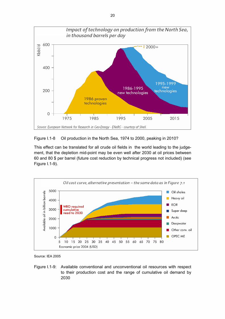
20

Figure I.1-8 Oil production in the North Sea, 1974 to 2000, peaking in 2010?

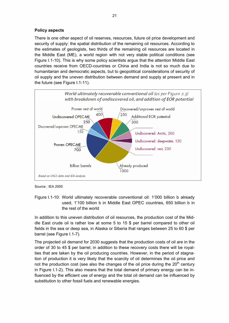
This effect can be translated for all crude oil fields in the world leading to the judge-ment, that the depletion mid-point may be even well after 2030 at oil prices between 60 and 80 $ per barrel (future cost reduction by technical progress not included) (see Figure I.1-9).

Source: IEA 2005

Figure I.1-9: Available conventional and unconventional oil resources with respect to their production cost and the range of cumulative oil demand by 2030

21

Policy aspects

There is one other aspect of oil reserves, resources, future oil price development and security of supply: the spatial distribution of the remaining oil resources. According to the estimates of geologists, two thirds of the remaining oil resources are located in the Middle East (ME), a world region with not very stable political conditions (see Figure I.1-10). This is why some policy scientists argue that the attention Middle East countries receive from OECD-countries or China and India is not so much due to humanitarian and democratic aspects, but to geopolitical considerations of security of oil supply and the uneven distribution between demand and supply at present and in the future (see Figure I.1-11).

Source : IEA 2005

Figure I.1-10: World ultimately recoverable conventional oil: 1’000 billion b already used, 1’100 billion b in Middle East OPEC countries, 650 billion b in the rest of the world

In addition to this uneven distribution of oil resources, the production cost of the Mid-dle East crude oil is rather low at some 5 to 15 $ per barrel compared to other oil fields in the sea or deep sea, in Alaska or Siberia that ranges between 25 to 60 $ per barrel (see Figure I.1-7).

The projected oil demand for 2030 suggests that the production costs of oil are in the order of 30 to 45 $ per barrel; in addition to these recovery costs there will be royal-ties that are taken by the oil producing countries. However, in the period of stagna-tion of production it is very likely that the scarcity of oil determines the oil price and not the production cost (see also the changes of the oil price during the 20th century in Figure I.1-2). This also means that the total demand of primary energy can be in-fluenced by the efficient use of energy and the total oil demand can be influenced by substitution to other fossil fuels and renewable energies.

22

0

200

400

600

800

1000

Afrika Nord Amerika Süd Amerika Asien Europa Mittlerer Osten Ozeanien

Produktion Verbrauch

Figure I.1-11 The uneven regional distribution of oil production and oil use, in million tons per year

Africa and the Middle East produce an enormous surplus of oil that is absorbed by the industrialised and emerging countries in North America, Europe and Asia (see Figure I.1-11). The patterns of production and consumption of natural gas are similar to those of the oil, the difference being that

• the exploitation started about 50 years later,

• the natural gas is more difficult to transport reflected in not one world market, but in three regional markets (North America, Africa, and Europe/Asia) deter-mined by the transportation by pipelines. This will change in the future by liq-uefied natural gas.

• the ratio of proven reserves to yearly consumption is now 60 years due to the faster increase of gas production that was 2.0 % per year during the last 15 years (oil: 1.3 % per year).

• the distribution of natural gas over the earth is somewhat better than for oil, but not too much as natural gas fields often go with fields of conventional crude oil. The largest resources of natural gas are again in the Middle East, which expects increasing world market shares in oil (see Figure I.1-12) as well as in natural gas some decades later.

23

50

63

16.5

25.929

35

24.1

27.9

39.7

42.5

37.1

49

0

10

20

30

40

50

60

70

1980 1990 2000 2010 2020 2030

Zeit

Prod

uktio

nsan

teil

an d

er

Wel

terd

ölfö

rder

ung

OPEC insgesamt

Naher Osten (OAPEC)

World oil production 1985-2020. Source : CEPE, 2001

world oil proven reserves 2000• Saudi Arabia 25.3% • Iraq 10.8%• Kuwait 9.3%• Arab Emirates 9.2%• Iran 8.7%• Qatar et al. 3.0%• Middle East 66.3%

Middle East

totalSh

are

of o

il p

rodu

ctio

n of

glo

bal p

rodu

ctio

n

time

Figure I.1-12 Re-concentration of oil production in the Near East, owning two thirds of global oil resources

Concluding remarks Looking at the period of industrialised countries in a very long perspective of mankind the use of oil and other fossil fuel will be not more than an episode which was first spelled out by M. King Hubbert in 1949 (see Figure I.1-13).

-10 -8 -6 -4 -2 heute 2 4 6 8 10

20

40

60

80

100

Erd

ölve

rbra

uch

(in b

elie

bige

n E

inhe

iten

Zeitabstand von heute (in Tausenden von Jahren)

0

World oil production and use seen in the geological periods

(according to M. Hubert, 1949: the Hubbert`s pimple)

Time from today (in 1000 years)today

Oil

cons

umpt

ion

(in a

nyun

it)

-10 -8 -6 -4 -2 heute 2 4 6 8 10

20

40

60

80

100

Erd

ölve

rbra

uch

(in b

elie

bige

n E

inhe

iten

Zeitabstand von heute (in Tausenden von Jahren)

0

World oil production and use seen in the geological periods

(according to M. Hubert, 1949: the Hubbert`s pimple)

Time from today (in 1000 years)today

Oil

cons

umpt

ion

(in a

nyun

it)

Figure I.1-13: The peaking of the world use of fossil fuels within a few centuries

24

The conclusions of these considerations are as follows:

• Oil resources will be available for far more than 100 years, so will natural gas and coal. But oil production is likely to peak within the next 30 to 40 years which is critical from the macro economic point of view threatening the eco-nomic development of the emerging and developing countries.

• The critical moment is not the moment of depletion of a non-renewable re-source, but after its depletion mid-point, if shrinking oil product demand is not in line with shrinking oil production; if there is a mismatch, high price in-creases of oil have to be expected.

• The uneven distribution of oil (and of natural gas) resources will give raise to many political tensions in the future, particularly in the Middle East, question-ing continuous economic development and social sustainability at a global level.

• The question of resource availability for future generations is not critical for fossil fuels, but extremely critical from the point of view of CO2 emissions: the critical question is where to dispose the CO2, as even at present emission rates mankind would need three atmospheres to avoid unsustainable climate changes (see Chapt. 1.2).

• Energy price increases in the 1970s demonstrated a stagnation of per capita primary energy demand for at least 15 years. This is a good message when world population stops growing which is expected in the second half of this century.

I.2. Energy Statistics If energy use increasingly becomes an issue of major concern, the measurement of energy use also gains importance. This means that policy makers and companies need solid information on energy use of the various kinds, their conversion efficien-cies and substitution potentials and their cost and prices; but all this implies clear definitions of the energy itself at the national and international level. Some of the en-ergy terms used are likely to be misunderstood due to traditional wording in different communities, branches and disciplines. Generally, a distinction is made at three lev-els:

(1) Primary energy, where two interpretations are possible: - the physical definition: Energy recovered from natural resources, but not con-verted by any succeeding process, i.e. crude oil, hard coal, natural gas, gas from coal mines, lignite, solar energy, wind, hydro power, fire wood, geothermal energy, wave energy, and uranium ores; - the energy economics definition: energy that is produced domestically or im-ported to a country; this can be primary energy in the physical sense or con-verted forms of energy (e.g. oil products like heating oil, gasoline, electricity). Industrial or municipal wastes being burnt in large boilers may also be consid-ered as primary energy as well as methane from landfill, sewage plants or fer-mentation plants.

25

(2) Final Energy any energy that is used by end users such as private households, services, in-dustrial companies, car drivers, trams, or trains mostly sold via markets, Final energy may also be heat generated by solar collectors or wood collected pri-vately in (private or public forests), or bio-ethanol from agricultural crops.

(3) Useful energy this form of energy is energy after the conversion of the final energies, e.g. heat from radiators, power transmitted to the axis of a car, light coming from a bulb, or the information and transformation in electronic devices and appliances.

(4) Energy Service Finally, the obvious purpose of the impact of the useful energy is called the en-ergy service which may be a comfortable room, a cooked meal. a transport from A to B, a ton of steel or cement, a beer bottle or a newspaper.

The mere data on energy use of these different forms on a national level may not be comparable, because most of them are gathered by observing their flow via markets. In rural areas, and particularly in developing countries, however, energies like fire-wood or dung are only partially traded; much is simply collected by the end user.

Having distinguished these three levels of energy use, one can ask about today’s losses of a national or continental energy system (see Figure I.2-1).

Space Heat 52,200

Process Heat 49,800

Other Drives 20,500

Illumination 800

Information, 1500Communication

Motive Power 14,100

Useful Energy of Final Energy Sectors

9,500 PJ non-energetic use

Final energy 294,800 PJ

Primary energy447,150 PJ

Industry 97,000 PJTransportation 79,000 PJPrivate households 79,200 PJTrade, commerce, 39,600 PJEtc.

143,650 PJ

Transformation losses

Energy Services

Heated Rooms(

Industrial Products

Mobility

Automation,Cooling

Illuminated Areas (

PC-, Phone- andInternet Use

in m )

(in tons)

(in Pass.km)

in m )

2

2

Losses for generating useful energy

Useful energy (incl. 7400 PJ distribution losses)

PJ

Sources: OECD 2005, ISI Karlsruhe140,800 154,000 PJ

Plastics,Asphalt

32.1%31.5% 34.5%

Figure I.2-1 Energy Flow Diagram for the World 2003

Energy losses can be distinguished on four levels, three of them are energy losses and the fourth is inefficient use of energy-intensive materials and too heavy moving parts and vehicles:

• Today, more than 440’000 PJ per year of global primary energy demand de-liver almost 300’000 PJ of final energy to customers, resulting in a loss of al-most 145'000 PJ for power generation, refineries, coke making and losses for

26

distribution and transmission. The largest losses stem from thermal power plants with efficiencies around 30 to 40%.

• The conversion of final energy to useful energy in boilers, engines, electrical motors, furnaces, kilns, and bulbs or computers generate losses of 155'000 PJ. The poorest efficiencies being in road transportation between 20 and 30% (and bulbs with 5 to 10 %). Thus, 250’000 PJ or two-thirds of primary energy demand is presently lost in energy conversion, mostly as low- and medium-temperature heat (UNDP/WEC/UNDESA, 2000). The conversion efficiencies of the Swiss transformation sector are somewhat better due to high shares of hydropower.

• The losses at the useful energy level sum up to 140'000 PJ, again almost one third of the primary energy. High losses are in the buildings sector and indus-trial process heat. These energy losses that are scarcely mentioned (pres-ently almost 39% of the Swiss primary energy demand) could be substantially reduced or even avoided through such technologies as low-energy buildings, membrane techniques or biotechnology processes instead of thermal proc-esses, and lighter vehicles or re-use of waste heat.

• The last level is reducing the demand of useful energy by avoiding large de-mand of energy-intensive materials such as steel, aluminium, paper, plastics, copper, glass etc. In addition to this material efficiency by better construction, improved material properties and recycling there are further options such as substitution of these materials by biomass based materials (wood, starch, natural fibres) or by pooling of products and machines which are not very much operated by a single owner, such as harvest and construction machines (renting) or cars and light trucks (car sharing). This potential of indirect energy efficiency is about 0.5 % per year or 2'200 PJ per year globally (or twice the present primary energy demand of Switzerland).

Energy conversion coefficients

Energy use and losses are measured in very different scales what has to be under-stood by historical reasons. The English system (including the USA and the Com-monwealth) developed differently from metering systems at the European continent in the 19th and 20th century. In addition, special sectors like the oil or coal sector developed its own measuring systems such as Mtoe (million tonnes of oil equivalent), barrels, or Mtoe (million tonnes of coal equivalent). Although, presently accepted en-ergy measures are only Joules and kWh by international convention, the traditional systems still prevail in many countries and even international institutions such as the International Energy Agency (IEA) or the European Statistical Office (Eurostat). Therefore, some conversion factors are mentioned here to facilitate reading interna-tional and national energy statistics (see Table I.2-1).

The typical energy flow in energy statistics has the opposite direction as shown in Figure I.2-2, because the traditional energy economics perspective starts from supply and not from the energy demand-inducing drivers of an economy or private house-holds.

27

Table I.2-1 Energy statistics – energy conversion factors

Unit Conversion to joules (multiply by …)

Remarks

calorie (cal) 4.1868 Old unit for quantities of heat

ton-of-oil-equivalent (toe) 41.868 · 109 Defined as 107 kcal. The toe is widely used in international energy statistics

barrel-of-oil-equivalent (boe)

approx. 6.1 · 109 Conversion values range from 6.06 to 6.12 · 109

ton-of-coal-equivalent (tce)

28.6 · 109 Used as the main unit of energy in China

kilowatt-hour (kWh) 3.6 · 106 Used mainly for electricity

British-thermal-unit (BTU) 1.055 · 103 Used in the USA: other units include the therm (105 BTU) and the quad (1015 BTU)

watt-year (Wyr) 31.5· 106 Useful unit for analytical applica-tions: if one uses 1 W on average, one uses 1 Wyr in a year

Source: Gesamtenergiestatistik der Schweiz 2005 (Joint Energy Statistic of Switzerland)

28

Figure I.2-2 Energy Flow Diagram of Switzerland 2005

Energy consumption data of countries or other entities vary from year to year be-cause of several reasons:

• Changes in activity levels (number of people, number of households, electri-cal appliances, or cars, person kilometers, ton kilometers, number of jobs, tons of steel). These influences can be considered by defining specific energy demand which takes the change of drivers into account.

• Change of yearly weather fluctuations (cold/warm winter; moderate/hot sum-mer) has to be adjusted by heating degree days and cooling degree days. Heating degree days: are number of days below 12°C multiplied by the differ-ence between 12°C and the average temperature of those days (Switzerland: 3600; France: 2300; Scandinavia 4400 to 6000 heating degree days). The correction of the final energy which is used for heating is corrected by the fol-lowing formula:

Final Energyheating, I, corr = Final energyheating, i . HDDav30 / HDDi

where HDDav30 is the 30 years average heating degree day figure and

HDDi the actual heating degree day figure

The same correction is made for electricity demand regarding cooling degree days which is more important in warm climates. The cooling degree days above 25°C are about 80 for Zurich, 300 for Milano, and more than 1000 for subtropical and tropical regions. They may gain more importance in the next decades due to the greenhouse effect of climate change.

Weather can influence primary energy by 1 to 2%

• Short term fluctuations of industrial structures (particularly during the phases of the business cycles in industry sectors by different growth of the energy-intensive basic goods industries). In the take off period manufacturing indus-tries order more steel and other energy-intensive basic material than in the down swing period when it is unclear how much market demand will shrink. The business cycle can influence primary energy by 0.5 %

Often used energy indicators

In order to characterise the level energy use or the performance in efficiency terms, energy statistics use typical energy indicators such as the following often applied ones:

1. Primary energy intensity is defined as the relation of primary energy use per unit of GDP (which can be expressed for international comparison in exchange rates

29

or purchasing power parity (Switzerland: 3.140 GJ/CHF2004)). (See also the dy-namics of energy intensities for various countries in Figure I.2-3).

2. Final energy intensity is defined as the relation of final energy use per unit of GDP. (Switzerland: 730 GJ/CHF2004).

3. Per capita primary energy use. (Switzerland: 160 GJ/capita).

4. Per capita final energy use. (Switzerland: 117 GJ/capita).

5. Share of imported primary energy (import dependence is defined as the sum of domestically produced primary energy (e.g. natural gas, coal, oil, hydro, refuse, wood, solar, wind) relative to primary energy demand of a country): Switzerland: 54 %

Ener

gy in

tens

ity [M

J/D

M '8

5 G

DP]

1860 1900 1950 2000 2050

China

Great Britain

Germany

France

Japan

FormerSoviet Union

India

Eastern Europe

35

15

20

25

30

0

5

10

Expected trend developmentDevelopment for high capitaland technology transfer

Countries withstate trade

Germany referenceGermany CO2-reduction of 80%

Time

Source: Chandler et al., 1990; CEC, 1996; calculations (with monetary parity) by ISI, 1997

Figure I.2-3 Development of the primary energy intensities of different countries, 1860-2050

Primary energy Intensities of countries

The dynamics of energy intensities of countries have quite typical patterns (see Figure I.2-3):

• With increasing industrialization, motorization, and automation (including pri-vate households) energy intensity increases, before it passes a maximum, and is reduced by increasing shares of GDP contributed by the service sec-tors.

• The decline of energy intensity is caused by several effects: the growth of the service sector and saturation in building up the basic capital stock and infra-structure of a country. In addition, there may be saturation in energy intensive consumer goods such as electric appliances and cars.

30

• The maximum of energy intensity of a proceeding industrializing country is not reached by a later industrializing country due to know-how and technology transfer.

• Energy intensities of OECD countries declined by 0.5 to 1.8 % per year during the last 15 years, while former centrally planned economies reduced their en-ergy intensities between 3.6 % (Russia since 1995) and 6% annually (China).

• The relatively high primary energy intensities of countries in economic transi-tion in the 1980s and thereafter are due to two facts: (1) The Gross Domestic Product (GDP) values are expressed in Market Exchange Rates (MER) which underestimate the standard of living and the related energy services (2) The former centrally planned economies considered energy as public good and energy use was either without any cost or at very low subsidised levels lead-ing to very wasteful investments and behaviour in energy use.

Converting national currencies into one common currency

There are some notable differences when converting national currencies to one cur-rency such as US$ or Euros by Market Exchange Rates (MER) or Purchasing Power Parities (PPP). However, the differences may not be over-estimated when investigat-ing income effects between countries with similar standards of living. If the under-standing of the global economy comes from a conceptualization and modeling at the level of individual economies, subject to common influences (oil prices, information, FDI, US interest rates, US$-yen, US$-Euro etc exchange rates) then it is clear that:

• each country's development is partly based on engaging with international trade, so that its citizens' purchasing power is partly based on what they can purchase from abroad (using MER exchange rates) and partly based on do-mestic incomes and prices, and therefore partly based on PPP-type prices;

• in comparing countries, MERs can be very misleading because (a) they re-flect temporary factors irrelevant to purchasing power, such as speculation, and (b) the MER's do not provide a good indication of the level or growth rates for the mix of products bought by the lower income, usually rural, households. (There are many issues here, e.g. the rural households may rely on non-marketed traditional agricultural products, and these will not be in MER, and may be badly covered by PPP.)

• In comparing countries, PPP becomes increasingly irrelevant as people in-creasingly satisfy their basic needs; after a certain threshold, the happiness literature shows convincingly that higher incomes do not bring much more happiness; since the PPP/MER debate is about welfare, this implies that GDP per head on a PPP basis is less relevant at higher income levels than GDP per head on a MER basis, since the MER-GDP allows spending to be valued at world prices.

31

I.3. Ecological Economics and the concept of sustainable development

Neoclassical economics consider the natural resources as rather independent for the economic system (see Figure I.3-2). The resources taken out from the earth are only priced with production cost at the margin, and sometimes by royalties representing the fact that some capital has to be gained. This is needed to substitute the use of natural resources by capital investments (more efficient use, substitution by another resource, and another source of income for the producing country; see Dubai in con-trast to many other oil producing countries such as Nigeria, Algeria, Venezuela).

The release of wastes or rest emissions into the environment has generally no price (e.g. rest of water pollution such as salts, non-degradable chemicals, hormones; rest of air emissions: release of greenhouse gases, NOx, SO2, small particles).

Ecological economics try to assess the economic value of those streams of masses (see Figure I.3-1) taken out of the earth or deposited back into the environment by estimating the cost for substituting the non-renewable natural resource, the external cost of emissions, or by using the cost for avoiding the emissions as shadow prices.

Market forproductioninputs, e.g.

labour, capital

Marketfor goods

and services

Money

Goodse.g.

labo

ur

e.g. salaries, wages

e.g. subsidies

e.g. taxes

e.g. social securitybenefits

e.g. taxes

Companies

Public authorityat federal,

regional andlocal level

PrivateHouseholds

Natural resources

Natural environment Natural

environment

foreign producers foreign consumers

Market forproductioninputs, e.g.

labour, capital

Marketfor goods

and services

Money

Goodse.g.

labo

ur

e.g. salaries, wages

e.g. subsidies

e.g. taxes

e.g. social securitybenefits

e.g. taxes

Companies

Public authorityat federal,

regional andlocal level

PrivateHouseholds

Natural resources

Natural environment Natural

environment

foreign producers foreign consumers

Figure I.3-1 Cycle of money and goods in an economy – a simplified circular model

Economics of natural resources

Non-renewable resources recovered by mankind will gradually shrink and will have to be substituted by some other natural resource. The use of a non-renewable natural

32

resource may be substituted by a more intelligent use of it (efficiency strategy) using additional capital (and/or labour and know-how). Or it may be substituted by another material that however will undergo the same path of scarcity as long as it is a non-renewable natural resource.

When these substitution processes occur, the rule of Hoteling says that the price of the scarce resource (e.g. crude oil) increases by the interest rate of public institutions which is around 3% per year. This may not be reached in reality in many cases as the technological progress reduces the recovery cost in the order of 1% annually.

Given this situation of scarcity of non-renewable natural resources, there are two possibilities to handle the problem:

• the search for a renewable natural resource, or

• the substitution of natural resources by capital and know-how to ever improv-ing efficiencies.

The only available renewable natural resource – the back stop technology

The sun is the only “renewable resource” (for a longer period of some thousands or even billion years, see Figure I.3-2). The sun delivers in its direct or indirect forms (wind, hydro, wave power, bio-mass) the only natural resource on which mankind can draw upon for millions of years in the future. The energy amount of the sun's radia-tion falling onto the earth is many times higher than the present global primary en-ergy demand. the question is more how to collect this supply of abundant energy in an economic way, i.e., without applying too much resources of capital and labour.

Economy

GeologyClimate

Flora Fauna

Sun

Purification of solar radiation(P. Kesselring)

- 6Efficiency factor

„Bread“: Hydropower 10„Wine“: Carbon cycle Biomass 10- 3

„Cognac“: Biomass Hydrocarbon 10- 8

GeologyClimate

Flora Fauna

Climate and mountains

EconomyEconomy

GeologyClimate

Flora Fauna

GeologyClimate

Flora Fauna

SunSun

Purification of solar radiation(P. Kesselring)

- 6Efficiency factor

„Bread“: Hydropower 10„Wine“: Carbon cycle Biomass 10- 3

„Cognac“: Biomass Hydrocarbon 10- 8

GeologyClimate

Flora Fauna

GeologyClimate

Flora Fauna

Climate and mountains

Figure I.3-2 Ecological Economics – in contrast to neoclassical economics ecologi-cal economics are considering the economy as part of the natural en-vironment

The efficiencies of solar radiation are low (between 0.1% to 10-8; see Figure I.3-2), but the production cost of these forms of primary energy are either zero or ranging in cost categories similar to those of non-renewable energy uses. As the conversion of

33

non-renewable fossil energy use was very convenient in the past and related conver-sion technologies quite advanced and cheap, the new technologies of converting direct and indirect forms of solar energy into final energies are often quite costly. However, those renewable energy technologies with some decades of experience have experienced quite substantial cost reductions due to learning and economies of scale (see Figure I.3-3).

Figure I.3-3 Development of cost of electricity generation of photovoltaics, wind energy, solar thermal power plants, and electricity from bio mass as function of yearly power generation in relation to constant electricity generation costs of conventional power plants (at present and in the future with carbon capture and storage (CCS).

The starting values of the cost ranges refer to the present global electricity genera-tion by these technologies (except conventional thermal power generation at the ba-sis (see Figure I.3-3). The ends for wind and biomass may be overstated and may end at the 100% line. The decline of the generation cost results from the observed experience curves that include learning and economies of scale effects (e.g. Photo-poltaics: -20% cost reduction for each doubling of generation; biomass between -5 % and -15 % as a range of uncertainty). The percentages reflect the share of today’s electricity demand.

The new renewable energies can also be considered as "back stop" technologies as they limit the application of fossil fuels in the next decades if fossil fuels, particularly oil, experience rising production cost (tertiary recovery, see Chapt. I.1) and rising prices and politically uncertain availability of the crude oil in the Middle East where two thirds of the remaining resources are located (see Figure I.3-4). On the other

34

hand, it is expected that renewable energies have declining prices and production cost (see above). As fossil fuels have high external cost (see below) these costs have either to be internalised or renewables should have some financial incentives to level the economic playing field of the technologies and also the option of more effi-cient energy use.

There are many forms of renewable energies (see Figure I.3-5) such as the direct forms of thermal and photovoltaic solar use or many indirect forms such as hydro power, wind power, various applications of biomass such as wood, fermentation of biomass, and other forms such as wave power. Geothermal energy is a further form of "almost" renewable energy.

50

63

16.5

25.929

35

24.1

27.9

39.7

42.5

37.1

49

0

10

20

30

40

50

60

70

1980 1990 2000 2010 2020 2030

Zeit

Prod

uktio

nsan

teil

an d

er

Wel

terd

ölfö

rder

ung

OPEC insgesamt

Naher Osten (OAPEC)

World oil production 1985-2020. Source : CEPE, 2001

world oil proven reserves 2000• Saudi Arabia 25.3% • Iraq 10.8%• Kuwait 9.3%• Arab Emirates 9.2%• Iran 8.7%• Qatar et al. 3.0%• Middle East 66.3%

Middle East

total

Shar

e of

oil

pro

duct

ion

of g

loba

l pro

duct

ion

time

Figure I.3-4 Re-concentration of oil production in the Middle East, owning two thirds of global oil resources and proven reserves

35

wood

rain

Solar radiation

CoalOil

Natural gasWood

HydropowerWave energy--Wind

Sun

climate system

substancesorganic

mill. of years wood

rain

Solar radiation

CoalOil

Natural gasWood

HydropowerWave energy--Wind

Sun

climate system

substancesorganic

mill. of years

Figure I.3-5 The sun as the most important energy source for the future and its different forms of direct and indirect solar energy

The unsustainable use of fossil energies today

In addition to conventional emissions, which have been in the focus of environmental policy in the 1960s to 1980s in industrialised countries and still are of major impor-tance in emerging countries and mega cities in developing countries, the CO2 emis-sions from fossil energies gained major attention during the last 20 years (Toronto Conference in 1987).

While the traditional emissions get washed out by the next rain or snow, the CO2

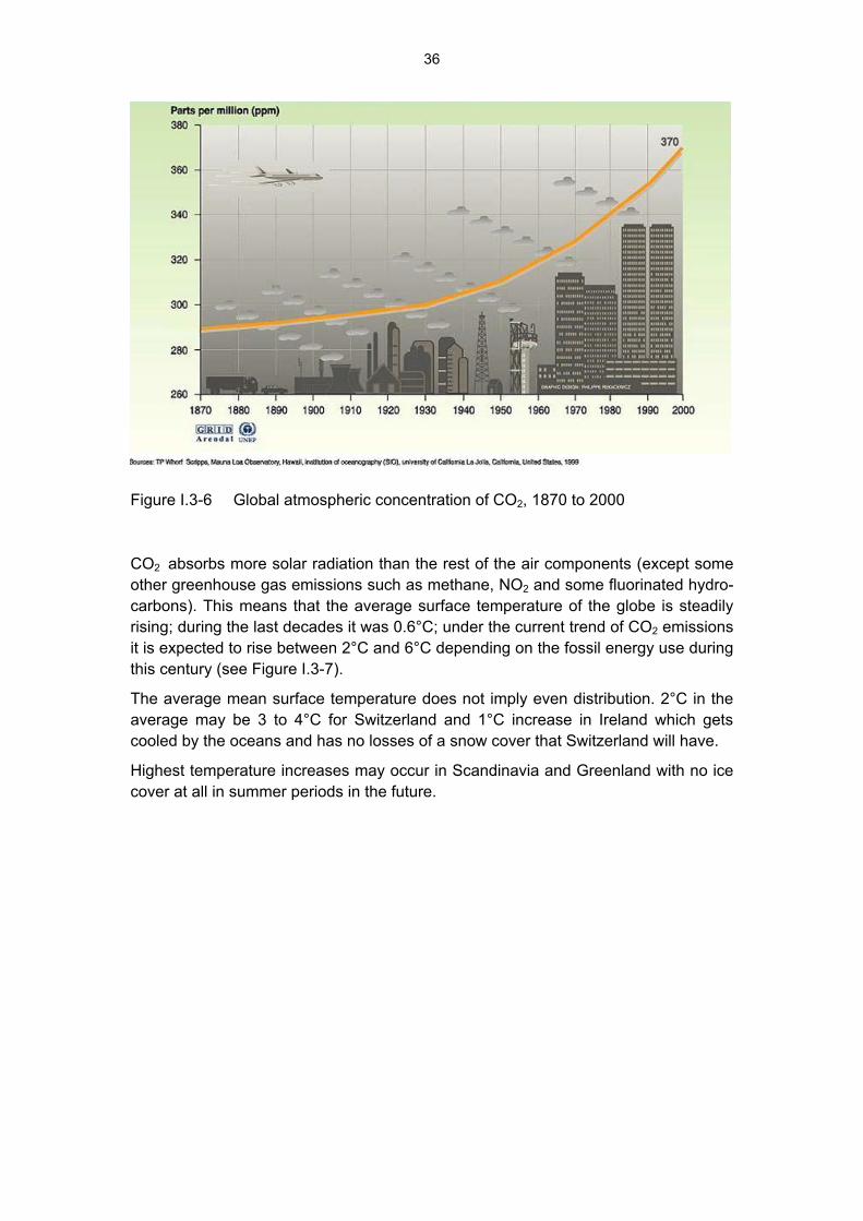
emissions remain for several hundred years in the atmosphere, before most of them gets absorbed by the oceans covering about 90% of the earth’s surface. As the life time of CO2 is so long and the emissions so high atmospheric concentration has in-creased since 1880 by 40 % from 270 ppm to 384 ppm in 2006 (see Figure I.3-6)

36

Figure I.3-6 Global atmospheric concentration of CO2, 1870 to 2000

CO2 absorbs more solar radiation than the rest of the air components (except some other greenhouse gas emissions such as methane, NO2 and some fluorinated hydro-carbons). This means that the average surface temperature of the globe is steadily rising; during the last decades it was 0.6°C; under the current trend of CO2 emissions it is expected to rise between 2°C and 6°C depending on the fossil energy use during this century (see Figure I.3-7).

The average mean surface temperature does not imply even distribution. 2°C in the average may be 3 to 4°C for Switzerland and 1°C increase in Ireland which gets cooled by the oceans and has no losses of a snow cover that Switzerland will have.

Highest temperature increases may occur in Scandinavia and Greenland with no ice cover at all in summer periods in the future.

37

High :18400 EJ conventional oil, 13000 EJ natural

gas, phase out nuclear by 2075

Constant aerosol concentrations beyond 1990 and high climate sensitivity of 4.5 °C

Low :8000 EJ conventional oil, 7900 EJ natural gas,

nuclear costs decline by 0.4% annualy

Constant aerosol concentrations beyond 1990 and high climate sensitivity of 1.5 °C

The 2 middle curves :12000 EJ conventional oil, 13000 EJ natural

gas, solar costs fall to 0.075$/kWh, 191 EJ ofbiofuels available at 70$/barrel

Upper curve : Constant aerosol concentrations beyond 1990 and climate sensitivity of 2.5 °C

Lower curve : changes in aerosolconcentration beyond 1990 and climatesensitivity of 2°C

Figure I.3-7: Temperature increase of mean surface temperature, global average

Sea level rise commitment : thermal expansion and land ice melt over 900 yearsafter an initial 1% increase in CO2 for 70 years, source IPCC, 1995

Figure I.3-8: Sea level rise due to thermal expansion and melting ice over 900 years

38

Figure I.3-9 Impacts of climate change on various fields of nature, economy and society

I.4. The concept of sustainable development

Definition

The concept of sustainable development has appeared as an answer to the major risks generated by the deterioration of the environment quality which has risen from pollution and harmful effects with a heavy influence on climatic changes and losses of biodiversity. But it also took into consideration the uneven distribution of wealth and resource use among the industrialised and developing countries.

The concept, in its current acceptance, has spread over time since the beginning of the seventies. Its course is marked out by a gradual awakening through several is-sues among which:

• the OPEC petroleum crisis in 1973 and again in 1979/80,

• the discovery of the Antarctic ozone hole in 85 or,

• the accident of the nuclear power plant of Chernobyl in 86,

and important contributions from studies like:

39

• the report of the “Club de Rome” in 1971 which has highlighted the threat of natural resources exhaustion by an extrapolation of the economic growth over one century, or,

• “Stratégie mondiale de la conservation”1 in 1980 in which the term of sustain-able development has been used for the first time.

Various definitions followed one another until the consensus introduced by the Brundtland UN-Commission Report in 1987 whose work was confirmed in a formal way by the Conference of the United Nations for the environment and the develop-ment held in Rio de Janeiro in 1992.

The adopted general definition presents the sustainable development as a develop-ment "which meets the current needs without compromising the capacity of the future generations to satisfy their own needs". It delimits sustainable develop-ment as the intersection of three spheres by postulating that a development cannot be viable unless reconciling the three undissociable social, economic and ecological aspects.

sustainable

Figure I.4-1: Principle of sustainable development – as an accepted equilibrium of societal, economic, and environmental concerns of today and in the long term future

However, this consensus lies between two opposite visions of sustainable develop-ment, which are the strong and weak visions (see also Figure I.4-1).

Weak vision of Sustainable Development (from the view of economics)

The soft vision is an ecologist and natural science position which considers that eco-nomic and social development would not be effectively sustainable unless making the environmental issues as a priority and accepting laws of natural sciences such as the second law of thermodynamics. This point of view is based on:

1 UICN (Union Internationale sur la Conservation de la Nature), Gland, Suisse.

Social Economic

Environment

Sustainable Bearable Viable

Fair

40

• The fact that the capacities of the ecological system are not extensible; in par-ticular, the second law of thermodynamics says that for each energy use there is a loss of energy in the form of exergy; this means that capital cannot entirely substitute the use of energy, and energy will always be needed e.g. by using some forms of the solar radiation on earth.

• The irremediable character of the deterioration of the environment (more than the social issues) such as extinction of species, halt of the Gulf Stream.

• And the principle of precaution (without including any considerations for the development of future technologies); it is unclear when sudden changes in the biosphere occur which would accelerate climate change (e.g. fast death of boreal forests that new Southerly forests could grow).

This approach deals with the decision making process in a hierarchical way by con-sidering the environmental aspects or issues first as the principal criteria for the evaluation of a project. In general, the partisans of the strong vision militate for a radical change of the society.

Discipline Principle Limits

Environmental scientist Carrying capacity Definite / unalterable

Strong sustainability Limits of substitutability Economist

Week sustainability substitutability of different capital

Manager / World Business Council

Eco-efficiency / Product stewardship

No limits to carrying capacity

Many engineers More efficient is better Often only physical limits

Figure I.4-2 Different interpretations and visions of sustainability by various disci-plines and professional communities

Strong concept of Sustainable Development (from the economic perspective)

The strong concept corresponds to an economist approach, which argues that "the natural capital which is threatened by exhaustion is entirely substitutable over time by technological progress and financial capital" (see Figure I.4-4). The priority here is thus given to the economic aspects while considering that the environment (and so-cial) protection must be based on a strong economy that can cope with all resource and social problems.

These two opposite perceptions are also reflected, to a certain extent, on the level of the development policies of the industrialized countries, the countries in economic transition, and the emerging and developing countries (Figure III.4-3). The first will tend to give a relatively higher importance to the environmental and social aspects while the others are likely to focus on the economic aspects of their development. Of course, the perceptions of countries, politicians, and scientists will change over time.

41

Environmental Economic

Social

OECD countries

Transition-economies

Developing countries

Figure I.4-3 Social, environmental and economic aspects of development policies objectives of industrialised, transition-economies and developing coun-tries

energyuse combination at low energy prices and

present technology

combination at high energy prices and present technology

combination at high energyprices and future tehnology

present technology options

future technology options

needed capitalM:\CEPE Zürich\Vorlesung\Lausanne\SS-2004\Folien\Vorlesung 4\Vorlesung 4.ppt

Figure I.4-4 Substitution between capital and the use of natural resources

The relation between the use of natural resources and of capital can be considered in a wide range as a substitution relation: the more capital in the efficient use of a natu-ral resource is invested the less of this resource is needed (see Figure I.4-4). Tech-nological progress opens up new opportunities of efficient use of natural resources over time. However, there are the limitations from natural sciences.

There may also be limitations of social acceptability regarding differences of the use of natural resources and economic well being which may limit capital accumulation in the North of the globe (see Figure I.4-5). There may be even limits of social differen-tiation in a country given the fact that the energy use per capita in one country (like Russia 4 kW/cap and 23 kW/cap for the last and first 10% of the population) can dif-fer more than a factor of 5 (see Figure I.4-6).

42

2

2000 2050 2100

4

6

Anteil fossile Energieträger ~90%

Anteil fossile Energieträger < 30

kW/capita

Untere (Armuts-) Grenze ~ konst. (Ansprüche steigen, Wirkungsgarde auch

Trotz abnehmendem Anteil an fossilen Brennstoffen wird die, aufgrund von Klima-Modellrechnungen bestimmte, obere (ökologische) Grenze immer enger.

Figure I.4-5 Energy demand per capita and limits of social acceptability of the poor

Figure I.4-6 Energy use per capita in different countries and class of population

43

II. Drivers of Energy Demand

II.1. The energy flow diagram – starting at the energy ser-vices

People do not want to use energy, they want services like comfortable rooms, illumi-nated houses or streets over night, to comfortably move from one place to another, tasty and healthy food or a warm shower. If this service involves some energy to de-liver the service the energy is perceived as a necessary good, as a prerequisite to receive the service. This energy need is technology dependent: the average house needs about 150 kWh/m2 and year to deliver the comfortable rooms in the winter pe-riod, while a solar passive house needs only 15 kWh/m2 and year for the same com-fort level. The losses of space heat (at the level of useful energy) are almost half of the energy losses at this level of the energy flow (see Figure II.1-1).

The useful energy (heat at different temperatures, moving power for vehicles or elec-tric drives, illumination, electronic calculations) is produced by energy converting technologies from final energies (e.g. gas or heating oil boilers, internal combustion engines, electric motors, or bulbs). The largest losses occur in the engines and gear boxes of road vehicles (80 %) and in bulbs with even 90 % losses (see Figure II.1-1).

The final energy is delivered to the final energy consumer in form of heating oil, gaso-line, jet fuel, natural gas, electricity, district heat or wood chips by energy companies or energy trade. Final energies are produced in refineries, power plants, district heat generating plants or wood chip producing plants. The largest losses occur in the thermal power plants that have an average efficiency of 36 % in Europe (see Figure II.1-1).

For Switzerland, the losses of the transformation sector from primary to final energy are about one fourth and amount to 37 % and 38 % respectively for the conversion from final to useful energy level and for the losses of useful energy. Some of the en-ergy services can be reduced by more efficient use of material or material substitu-tion reducing the demand of metals, plastics or braking losses of moved parts and vehicles.

The primary energy demand of Switzerland was about 1.132 PJ in the year 2005 and the per capita primary energy use was about 155 GJ/cap. (1990: 151 GJ/cap). The highest share of oil and oil products in primary energy demand was 76 % in 1971 and was reduced to 48 % in 2005 which is still quite high in comparison to other Euro-pean countries. Natural gas was introduced in Switzerland in the early 1970s and has reached a share of 10,3 % in 2005. This demonstrates how slow the structure of pri-mary energy changes over decades, but also that per capita energy use remained constant over a period of 15 years as an example of an industrialised country.

44

Source: Schweizerische Gesamtenergiestatistik 2004, BFE

Figure II.1-1 From energy services to useful energy, final energy and primary energy demand, Switzerland 2004

45

Energy data are derived from many sources that generate the data in different ways and therefore, the energy data for the same sector and year of a country may change according to the source (see Table II.1-1). Grid-based energies (electricity, gas, and district heat) are mostly more precise than non-grid-based being distributed by vari-ous trade channels and companies who do generally not distinguish between cus-tomer groups in their statistics (heating oil, coal, wood). The data for grid-based differ as well because the identification of customer groups and sectors is differently made by surveys (which may also be made in intervals for several years) or made by the accounting schemes of the energy delivering companies. Therefore, it may be useful to use only the official energy balances of a country published by the relevant institu-tion (in Switzerland the Federal Office of Energy, Bundesamt für Energie, BFE).

Table II.1-1 Sectoral energy demand figures may have different statistical sources and may differ from each other

II.2. Energy efficiency potentials (theoretical, technical, societal/welfare economics, micro-economic, ex-pected potential)

This part gives first some empirical examples on efficient energy use in several sec-tors and for several technological areas in the past, before a second analytical part develops the concept of energy efficiency. The third part looks into the future report-ing the vision of the Board of the Swiss Institutes of Technology of the 2000 Watt society.

46

II.2.1 Empirical examples of efficient use of energy

The development of specific energy use of engine and illumination shows quite im-pressively the improvement of efficient use of energy during the last 150 to 300 years (see Figure II.2-1):

• The technical progress endures for very long time over decades and centu-ries which may include new technologies for the same energy service (e.g. candle, bulb, indiscendent light, diodes (LEDs)).

• The technical progress can be surprisingly constant over a very long time pe-riod. This can be observed for many technologies of which the information technology has been the most fascinating during the last 30 years.

candles

LEDs

Ener

gyef

ficie

ncy

in %

candles

LEDs

Ener

gyef

ficie

ncy

in %

Figure II.2-1 Long term efficiency improvement of turbines and illumination between 1700 or 1850 and 2000

Starting from the early 1950s, specific electricity demand of computers could be re-duced by about a factor of 100 each decade (see Figure II.2-2). If this development was half as fast the computer capacity installed in Switzerland would need 10 times the electricity which is consumed today globally (see B. Aebischer, H. Bradke, H. Kaeslin: Energie und Informationstechnik. ETH Bulletin, Nr. 276, Januar 2000).

The reason for this success was that the number of transistors on a chip was in-creased from 1,000 in 1970 to almost 100 Mill. in the year 2000 (see Figure II.2-3).

47

1 E- 10

1 E- 09

1 E- 08

1 E- 07

1 E- 06

1 E- 05

1 E- 04

1 E- 03

1 E- 02

1 E- 01

1 E+ 0 0

1 94 0 1 96 0 1 98 0 2 00 0

M U SIC

C r ay

P C

IB M 37 0/1 6 8

C D C 64 00 /65 0 0

C D C 16 04

E R M E T H

Z U S E Z 4

Figure II.2-2 Specific electricity demand of computer generations during the last six decades; decrease of 10-10

Source: http://www.intel.com/research/silicon/mooreslaw.htm

Figure II.2-3 Number of transistors on a chip (Moore: doubling in 12 → 24 months)

Another example is the heat demand of houses and buildings during the last 30 years. The energy efficiency progress is much slower due to the very long re-investment cycle when facades are refurbished every 30 to 50 years. Due to the en-ergy price increases in the 1970s, many efficiency improvements could be gained in buildings, window systems and boiler and burner technology as well as in control of the heating and air conditioning system of buildings (see example of German multi-family dwellings heated with heating oil: Figure II.2-4).

Specific heat demand of the building stock was reduced from an average of 430 kWh/m2 in 1970 to about 150 kWh/m2 in 2000. Several ordinances (e.g. building codes for new buildings, for boilers and the control of the heating system, the energy billing in multifamily buildings), the ecotax, and research and development contrib-uted to this success. It is interesting to observe, that the building codes for new build-

48

ings since 2000 equal the performance of demonstration buildings in the 1980s (see Figure II.2-4). Most challenging is the energy demand of passive solar houses and buildings that only have an energy demand of some 15 kWh/m2 and year.

Most sustainable are the more stringent building codes. It is foreseeable that the specific heat demand of the building stock in Middle Europe will be below 45 kWh/m2 in 2070, i.e. one tenth of the heat demand of the year 1970. The European commis-sion is urging the Member States to harmonise the building codes according to the different climates in Europe. This is a fascinating example of a major energy consum-ing sector on moderate climates.

Specific heating oil dem and in m ulti-fam ily dw ellings

1st buildingcode

2nd building codenew buildings

3rd. B .C . 4th B .C .

O rdinance on individual heat billing

N ew heatingsystem efficiency standards

Specific heating oil dem and in m ulti-fam ily dw ellings

1st buildingcode

2nd building codenew buildings

3rd. B .C . 4th B .C .

O rdinance on individual heat billing

N ew heatingsystem efficiency standards

Figure II.2-4 Development of specific heating oil demand in multi-family dwellings in Germany, 1970 to 2000, in kWh/m2.a, building standards and research and demonstration houses

The decrease in specific energy demand by new technologies can be observed as a result of decrease of specific final energy demand of the final energy sectors (see Figure II.2-5). Specific fuel consumption of industry in industrialised countries is de-creasing by more than 1 % per year while specific electricity demand is rather con-stant (or slightly decreasing) during the last two decades. This difference demon-strates a visible improvement of fuel efficiency, while the efficiency progress in the electricity use is often compensated by more automation and process changes to more electricity driven processes.

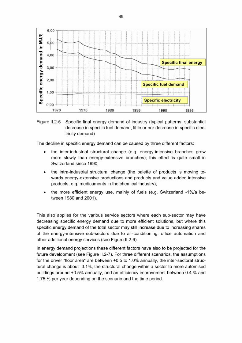
49

Specific final energy

Specific fuel demand

Specific electricity Spec

ific

ener

gyde

man

din

MJ/

€

Specific final energy

Specific fuel demand

Specific electricity Spec

ific

ener

gyde

man

din

MJ/

€

Figure II.2-5 Specific final energy demand of industry (typical patterns: substantial decrease in specific fuel demand, little or nor decrease in specific elec-tricity demand)

The decline in specific energy demand can be caused by three different factors:

• the inter-industrial structural change (e.g. energy-intensive branches grow more slowly than energy-extensive branches); this effect is quite small in Switzerland since 1990,

• the intra-industrial structural change (the palette of products is moving to-wards energy-extensive productions and products and value added intensive products, e.g. medicaments in the chemical industry),

• the more efficient energy use, mainly of fuels (e.g. Switzerland -1%/a be-tween 1980 and 2001).

This also applies for the various service sectors where each sub-sector may have decreasing specific energy demand due to more efficient solutions, but where this specific energy demand of the total sector may still increase due to increasing shares of the energy-intensive sub-sectors due to air-conditioning, office automation and other additional energy services (see Figure II.2-6).

In energy demand projections these different factors have also to be projected for the future development (see Figure II.2-7). For three different scenarios, the assumptions for the driver "floor area" are between +0.5 to 1.0% annually, the inter-sectoral struc-tural change is about -0.1%, the structural change within a sector to more automised buildings around +0.5% annually, and an efficiency improvement between 0.4 % and 1.75 % per year depending on the scenario and the time period.

50

0

100

200

300

400

500

600

1990 2000 2010 2020 2030 2040

w enig techn. m ittel techn. hoch techn. alle Büros

Ele

ctric

ityus

e[M

J/m

2 .a]

low techn. med. techn. high techn. all offices

0

100

200

300

400

500

600

1990 2000 2010 2020 2030 2040

w enig techn. m ittel techn. hoch techn. alle Büros

Ele

ctric

ityus

e[M

J/m

2 .a]

low techn. med. techn. high techn. all offices

Figure II.2-6 Possible evolution of specific electricity demand of all office buildings in Switzerland: fast decrease for individual types but first increase and later only slow decrease – due to „structural change“ (fraction of high tech buildings is increasing!)

-2.0

-1.5

-1.0

-0.5

0.0

0.5

1.0

1.5

2.0

2.5

3.0

90 — 95 95 — 00 05 — 1 0 15 — 2 0 25 — 30

Szenario I

Szenario I I

Szenario I IIa

Fläche

Strukturwandel 1

E.kennzahl hom . Gruppe

Strukturwandel 2

Auswi rkung auf den Energieverbrauch [J ährliche Veränderung in %]

Figure II.2-7 Contribution of four factors on energy demand of the service sectors (office area, inter-sectoral structural change, intra-sectoral structural change, efficiency improvements) to the annual variation of electricity demand in the service sector, in % per year

51

- Economic potentials of efficient solutions

Companies in industry and service have often high economic energy efficiency po-tentials, which energy managers mostly do not even know. Often these are old boil-ers, compressed air systems, steam systems and cooling applications that are over-designed in capacity, poorly maintained and since years not noticed. These are mainly energy technical off-side installations that are not directly relevant for the pro-duction (see Romm, 2000: Cool companies). There potentials are rather high varying between 25 % and 40 % and quite profitable in the light of internal rates of return between 15 % and 25 % (see Table II.2-1).

Table II.2-1 Examples of "no regrets" (profitable energy efficiency investments)

Type of off-site Efficiency potential Internal rate of investment 1)

11 MW air compressor station 30 % 20 %

25 MW heat and vapour generation 35 % 25 %

4 MW heat recovery for preheating glas row material and cullets

40 % 18 %

90 kW water circulation pumps 25 – 35 % 20 %

75 kW illumination of a storage and pro-duction hall

20 – 30 % 15 %

100 kW air compressor station (valves and control by staff)

25 % 20 %

1 MW waste heat use from plastic manu-facturing machines

40 % 18 %

1) including planning cost

Because the production plants are more in the focus of the management, energy efficiency potentials in the plants are often considered as being small; they are not so apparent and are only recognizable through more process know-how and can be realised by process substitutions.

The specific energy uses are very different in the enterprises of the processing branches or of the service sector even though the products are quite similar or even the same. There are various reasons for these differences:

• Compared to a new high tech plant many production and off-side plants are not yet depreciated and are running on an energy technical level of the 1980s or 1990s (economical within the existing plant).

• Installled capacity compared to today’s heat and power use (over-design), and poor planning of existing plants or not taking into account that using structures have changed, this can cause up to 30% energy use that has to be denoted as unnecessary use (typical examples are: boilers, steam distribution systems, air compressor stations, see Table II.2-1).

• Additionally, a bad operation management like idle running machines, too strong air conditioning or too high process temperatures can be often ob-served.

52

All this can cause an energy use double as high compared to a new, fully optimised plant at a new site (see Figure II.2-8)

Best practice plantPoorly managed plant

Best practice companies may use half of the energy of poorly managed plants

Poor operation

Poor capacity load

Bad planning, old technology

Good practice in existing plant

Economically feasible in a newly constructedplant

Best practice plantPoorly managed plant

Best practice companies may use half of the energy of poorly managed plants

Poor operation

Poor capacity load

Bad planning, old technology

Good practice in existing plant

Economically feasible in a newly constructedplant

Figure II.2-8 The influence of organisational measures on the energy demand of an existing plant and a new best practice plant (scheme)

A conclusion and further considerations (see Figure II.2-9):

• Even if energy techniques are demonstrably improving efficiency for decades a theoretical limit will be reached, but this can often be skipped by new tech-nology.

• However, at the level of energy use of industrial branches different effects are running in different directions (mechanisation/automation/higher comfort in-crease energy demand) that at first sight no improvement of energy efficiency can be detected (e.g. electricity intensity).

• Economists call the following the "stair case" effect. The energy efficiency im-provements that have been implemented in the OECD countries since the 1970s would be depleting in the coming decades and then energy use per capita would increase again like in the 1960s in the industrial countries.

• In contrast to that the ETH council described a vision of a 2000 W per capita society in 1998, that means a decrease of per capita energy use by two third compared to today’s level of 65 GJ/cap until the middle of this century, while the prosperity is increasing (ETH-Rat, 1988).

53

In the following paragraphs we investigate the technological developments of energy efficiency that would be necessary to achieve this long-term target and if the stair case effect that is mentioned by some economists is rather improbable.

On the basis of useful energy that has not much been in the focus so far many en-ergy losses could be avoided if the reasons were analysed in more detail (1) (see Figure II.2-9), the decrease of exergy was considered (2), the process substitution was taken into account (3), heat and kinetic energy were saved (4), and last but not least cost reduction possibilities were considered (5).

Figure II.2-9 Strategical measures of efficient energy use under five different technology perspectives

II.2.2 The analytical concept of energy efficiency

The potentials of efficient energy use (or also renewable energies) can be described under technical and economical aspects as follows (Goldemberg, 2000, vgl. Figure II.2-10):

54

• For a certain year in the future an energy efficiency potential exists that is thought to be reachable through re-investment and better management in the given energy economic environment (expected potential).

• Actually more energy efficiency investments would be profitable, but they are not realised because of different reasons (lack of knowledge, split incentives, lack of capital availability, poor decision processes, high transaction cost, market imperfections (external cost of energy use); this potential is called: mi-cro-economic potential. Here, energy policy can increase the expected poten-tial. When energy prices are rising, the economic efficiency potential is in-creasing too.

Theoreticalpotential

TechnicalpotentialExpected

potentialProfitable potential

Macro-economicpotential (includingexternal cost)

Externalcost

obstacles

Theoreticalpotential

TechnicalpotentialExpected

potentialProfitable potential

Macro-economicpotential (includingexternal cost)

Externalcost

obstacles

Theoreticalpotential

TechnicalpotentialExpected

potentialProfitable potential

Macro-economicpotential (includingexternal cost)

Externalcost

obstacles

Figure II.2-10 Concept of distinction of energy efficiency potentials – from the theo-retical to the expected efficiency potential

• External costs are affiliated with energy use. These costs are considered to be 2 to 5 Rp/kWh, but are not included in the energy prices. If they were, the potential of efficient energy use would be enlarged from a macro-economic point of view (macro-economic potential).

• Engineering and natural sciences are continuously expanding the technical energy efficiency potential by technical improvements or totally new technolo-gies and materials with low specific energy consumption. Only a part of the technical potential is economic, due to lack of experience and economies of scale of their production (the technical solution has to be at least realised in pilot plants or laboratory tests); this potential is called the technical potential.

• Many things could theoretically be operated more efficiently (e.g. membrane applications instead of thermal separation, foamed metals for moving parts etc.). But they first need to be technically realised in laboratories before they can be described as technically feasible (theoretical potentials). The theoreti-cal potential is estimated to be 80 – 90 % (Jochem, 1991).

55

In the past mostly energy conversion was in the focus of efficient energy use, e.g. energy plants, refineries, boilers, burners, gas turbines, combustion engines, electric motors, pumps, compressors or heat converters und pumps, and not reduction of useful energy, which has average losses of 37% (relating to primary energy use) in Switzerland. The examples in Table II.2-2 show technology substitutions (steel rollers, building insulation, separation of substances in individual processes, dyeing of tex-tiles) as well as improvement innovations (cars and movement controlled illumination or entertainment electronics). The technical potentials mentioned here show 40-60% in average that could be economic within the next 20 years (if they are not yet profit-able today).

Table II.2-2 Reducing useful energy demand via substitution of processes and avoiding heat losses

Efficiency improvement

• Thin sheet casting of steel instead of cast-ing

-30 to -50%

• Passive energy house with 20 kWh/m2.a -70% SIA 380

• Separation of material via membranes in-stead via thermal separation processes

-60 to -85%

• Dyeing with enzymes at 20°C instead at 140°C in a jet

up to -99%

• Reducing the weight of vehicles, and Cw value

-20 to -30%

• Movement controlled appliances instead of stand-by mode

-90 to -95%

Elevators in living and office buildings are examples to show how modern power electronics explore a totally new field of feeding back the brake power of electrically operated aggregates (see Figure II.2-11). The electricity demand can be reduced by 80% in this example compared to a conventional elevator, if the lift is operated by feeding back the electricity, high efficiency electric motor and a special gear system.

56

Quelle: Siemens, 1999

Figure II.2-11: Electricity demand of different elevator systems for buildings

Similar technologies are found in many fields where moving parts are decelerated. The more often this application is realised, the more economic the feed back of elec-tricity will become, e.g. in hybrid cars being introduced in 2005, rolling stairs, or many industrial processes.

Electricity generation in thermal power plants has losses between 40% (gas fired plants) and 65 % (nuclear plants). In addition, one has to take into account losses of transmission, storage (hydro storage plants), transformation, and distribution of about 8 %, before electricity can be used. If used for warming up low temperature applica-tions, the efficiency is extremely poor according to second law of thermodynamics at about 5 %. This is because the exergy content of electricity (or fossil fuels) could generate temperatures above 2.000°C and is, therefore, "over-qualified" for making heat at 40 to 70°C for heating purposes or warm water. This application of electricity may be convenient and at low investment cost, but at a few kW capacity these kinds of electricity use may be uneconomic and certainly a waste of energy from the view point of the second law of thermodynamics.

This poor exergetic efficiency gets even worse, if energy use is wasteful and un-known. The need for comfort and lacking knowledge of energy consumers addition-ally decrease the efficiency up to a factor of two; this sums up to an exergy efficiency of less than 3 % of electricity use in low temperature applications.

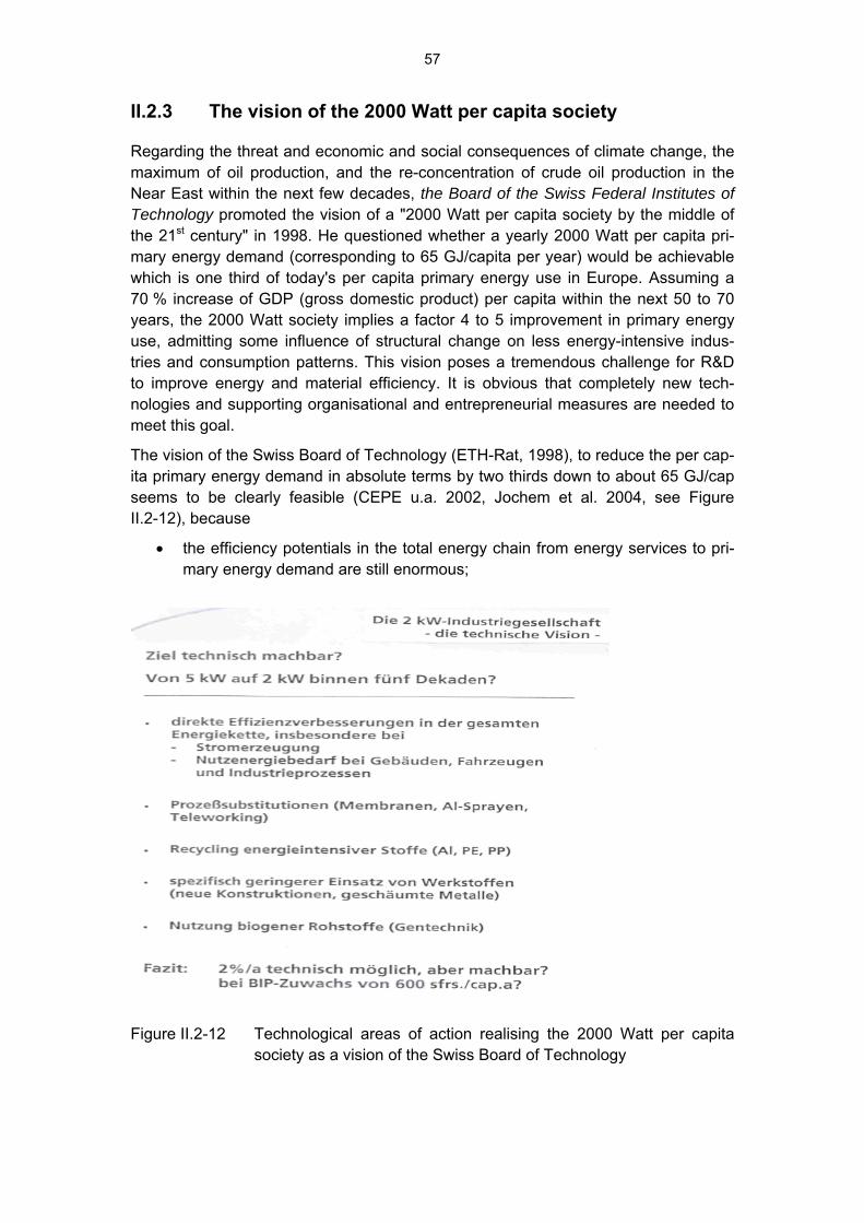
57

II.2.3 The vision of the 2000 Watt per capita society

Regarding the threat and economic and social consequences of climate change, the maximum of oil production, and the re-concentration of crude oil production in the Near East within the next few decades, the Board of the Swiss Federal Institutes of Technology promoted the vision of a "2000 Watt per capita society by the middle of the 21st century" in 1998. He questioned whether a yearly 2000 Watt per capita pri-mary energy demand (corresponding to 65 GJ/capita per year) would be achievable which is one third of today's per capita primary energy use in Europe. Assuming a 70 % increase of GDP (gross domestic product) per capita within the next 50 to 70 years, the 2000 Watt society implies a factor 4 to 5 improvement in primary energy use, admitting some influence of structural change on less energy-intensive indus-tries and consumption patterns. This vision poses a tremendous challenge for R&D to improve energy and material efficiency. It is obvious that completely new tech-nologies and supporting organisational and entrepreneurial measures are needed to meet this goal.

The vision of the Swiss Board of Technology (ETH-Rat, 1998), to reduce the per cap-ita primary energy demand in absolute terms by two thirds down to about 65 GJ/cap seems to be clearly feasible (CEPE u.a. 2002, Jochem et al. 2004, see Figure II.2-12), because

• the efficiency potentials in the total energy chain from energy services to pri-mary energy demand are still enormous;

Figure II.2-12 Technological areas of action realising the 2000 Watt per capita society as a vision of the Swiss Board of Technology

58

• energy-intensive use of mass materials can be still more intensively used in recycling cycles, but also used more efficiently by better materials and im-proved deign; they can also be substituted in many cases by biomass as their basic resource.

• the cost of the new technological solutions may be high at the beginning of their technology cycles, but may substantially decrease by learning and economy of scale effects.

Although the technological feasibility of the 2000 Watt society has a good perspective, the economic feasibility of this total conversion of the existing capital stock within some five to seven decades is still unclear. Even if this question could be answered positively in favour of the vision, there is still the question of political acceptability of such a vision. Private households make their investment decision more on the basis of preferences and social value systems of their social groups and far less by eco-nomic considerations. Presently, a rich family often prefers a heavy powerful car than an efficient light one as social acknowledgement is in favour of the inefficient car.

It remains open today whether a social acceptance of a 2000 Watt society will sup-port this development of a sustainable energy system or not (see Figure II.2-13).

Figure II.2-13 The vision of the Board of Swiss Institutes of Technology of a 2000 Watt/cap Society – the long term efficiency potential in 2060 to 2070

59

III. Energy Demand and Conversion – drivers, sectors, cost Introduction

This chapter covers the various aspects of future energy demand and supply projec-tions, the scenario design technique, the technological developments, and cost as-pects.

The basic equation of projecting future energy demand is quite simple and generally has the form of (see also Figure III-1):

energy demand of a sector i = specific energy demandi . energy driveri

which may be for industrial branches the value added or tons of products produced, for services it may be office area or employed persons, for transport it may be tonkm or personkm per year and for private households the living area or the number of electric appliances of the various types.

S pa c e He a t 2 25 7 6,4

P ro ce ss He at 8 2 ,0 5 5,6M o tive Po w e rt

O the r D rive s 5 2 ,8 6 0,6

Illu mina tio n 2 1 8 ,5

Info rma tio n, n.d. n.d.C o m m unica tio n

55 ,7 20 ,0

Nu tze n e rg ie d e r E n d e ne rg ies ek to ren

2 1 ,3 P J n on -en e rg e tic C on su mp tion

F in a l E n e rg y85 3 ,7 PJ

E nergy-F low D iagram for S w itzerland 2002

P rima r y e n e rg y1 .1 4 7 P J

In d us try 1 6 8 ,5 P JT ra nsp or ta tion 3 0 2 ,8 P J

P r iv a te Ho u seh o lds 2 30 ,6 P J

T ra de , C o m m er ce , 1 5 3 ,5 P J

2 7 1 ,8 PJ

Trans fo rm ation Los s es

E n e rg y Se rv ice s

He a te d R oo ms(in q m )

Indus tria l P ro duc ts (in to ns )M o bility(in P a ss .km)Auto ma tio n,C o o lingIllu mina te d Are a s(in q m)P C -, P ho ne - a nd Inte rne t Us e

2

L os se s fo r g en era tin g Us e fu l En er gyUs e fu l En ergy

(Inc l. 2 3 P J D is trib utio n L oss es )

P J

Sourc e: IS I, Kar lsruhe

Nu tz ung s-grad in %

4 2 9 P J 4 2 5 PJ

P las tic s ,A sp halt

K :\E \Dab a-al\E nergie flus s diagram m e\2002_en-E nerg iefluss Sc hweiz\2002E nerg ie fluss F o lie.ppt

2 4 ,1 %3 8 ,1 % 3 7 ,8 %

Drivers of theuseful energy level

X specificenergydemand

= final energydemand by final energy sectors

S pa c e He a t 2 25 7 6,4

P ro ce ss He at 8 2 ,0 5 5,6M o tive Po w e rt

O the r D rive s 5 2 ,8 6 0,6

Illu mina tio n 2 1 8 ,5

Info rma tio n, n.d. n.d.C o m m unica tio n

55 ,7 20 ,0

Nu tze n e rg ie d e r E n d e ne rg ies ek to ren

2 1 ,3 P J n on -en e rg e tic C on su mp tion

F in a l E n e rg y85 3 ,7 PJ

E nergy-F low D iagram for S w itzerland 2002

P rima r y e n e rg y1 .1 4 7 P J

In d us try 1 6 8 ,5 P JT ra nsp or ta tion 3 0 2 ,8 P J

P r iv a te Ho u seh o lds 2 30 ,6 P J

T ra de , C o m m er ce , 1 5 3 ,5 P J

2 7 1 ,8 PJ

Trans fo rm ation Los s es

E n e rg y Se rv ice s

He a te d R oo ms(in q m )

Indus tria l P ro duc ts (in to ns )M o bility(in P a ss .km)Auto ma tio n,C o o lingIllu mina te d Are a s(in q m)P C -, P ho ne - a nd Inte rne t Us e

2

L os se s fo r g en era tin g Us e fu l En er gyUs e fu l En ergy

(Inc l. 2 3 P J D is trib utio n L oss es )

P J

Sourc e: IS I, Kar lsruhe

Nu tz ung s-grad in %

4 2 9 P J 4 2 5 PJ

P las tic s ,A sp halt

K :\E \Dab a-al\E nergie flus s diagram m e\2002_en-E nerg iefluss Sc hweiz\2002E nerg ie fluss F o lie.ppt

2 4 ,1 %3 8 ,1 % 3 7 ,8 %

Drivers of theuseful energy level

X specificenergydemand

= final energydemand by final energy sectors

Drivers of theuseful energy level

X specificenergydemand

= final energydemand by final energy sectors

Figure II.2-1 Empirical observation looking at the energy flow and generalised equation for projecting future energy demand

The projection of future energy demand and supply is performed by quantitative models, often as model systems today. These model systems contain several types of models such as macro economic models simulating the future economic perform-ance of a national economy, process-oriented sectoral models (also called bottom-up models) which simulate future energy demand of sectors and sub-sectors, and finally specific modules linking the macro-economic and bottom up models together to a "hybrid" model (or the model system; see Figure III-2). These linking modules trans-fer the results of the macro-economic models into the drivers (often physical drivers such as floor area of single or multi family houses, floor area in the various sub-sectors of the service sector) of the bottom up models; or they feed back the informa-

60

tion on additional investments calculated by the bottim up models to the macro eco-nomic model (see Figure III-2)..

Transformation moduleE. Jochem (EJ)

Primary Energy

ConversionF. Noembrini

Co-generationF. Noembrini

Conversion Sectors etc.

Boundary Conditions – Data from the Database

Energy-efficientBoundary Conditions Macro-model

M. Wickart (MW)

Energy sectorsHousehold &

Electrical appliances G.

Catenazzi (GC)

ServicesG. Catenazzi

Industry E. Jochem

TransportationF. Noembrini (FN)

Cost moduleM. Wickart

Emissions

Modified Input, etc.

ConversionF. Noembrini

Co-generationF. Noembrini

Transformation moduleE. Jochem (EJ)

Primary Energy

ConversionF. Noembrini

Co-generationF. Noembrini

Conversion Sectors etc.

Boundary Conditions – Data from the Database

Energy-efficientBoundary Conditions Macro-model

M. Wickart (MW)

Energy sectorsHousehold &

Electrical appliances G.

Catenazzi (GC)

ServicesG. Catenazzi

Industry E. Jochem

TransportationF. Noembrini (FN)

Cost moduleM. Wickart

Emissions

Modified Input, etc.

ConversionF. Noembrini

Co-generationF. Noembrini

Figure II.2-2 Energy Navigator – an energy simulation model system at CEPE con-sisting of a macro economic model (Input-Output model), a transfor-mation module, several bottom up models and a cost module. This configuration is often called "Hybrid model")

III.1. Energy Sectors and Energy Chains This chapter describes the typical structure of bottom up models how the different energy using and producing sectors are structured.

III.1.1 Private Households

Generally, the energy demand of private households is divided into two sub-sectors, the energy demand for heating, cooling and warm water on the on hand, and electric appliances on the other (including lighting, communication and other electric uses).

Heating and cooling

Space heating is a major demand of final energy in the industrialised countries with moderate climates, where energy demand for cooling is almost non-existent. On the other hand, space cooling (including ventilation) may be the most important energy demand of private households with high per capita income in subtropical and tropical world regions. The energy demand for heating or cooling depends on the following

61

factors that have to be known for the existing building stock of a country and have to be projected:

• Heated (or cooled) floor area (if not available: number of households);

• Difference between indoor and outdoor temperature (degree days: medium temperature difference of a day below 16°C (heating) or above 25°C (cooling);

• Technology: insulation of the building (facades, roofs, basements, window systems), type of heat/cooling generation, control techniques for heating and cooling, heat/cooling distribution, heat/cool recovery;

• Behaviour of building users: ventilation, overheating or-cooling, management of control techniques driven by income, values, traditions.

Warm water generation and use

Warm water demand is very much dependent on income per capita and traditions in a country or social group. The efficiency of warm water generation has been very much improved and washing traditions have moved from taking a bath to taking a less energy-intensive shower; however, the habits of washing have substantially changed to more often showers and careless use of warm water in the industrialised countries. The demand for energy for warm water use is usually determined by

• the number of persons in a household and total population of a country;

• the technology: type of warm water generation, losses of distribution,

• behaviour: frequency and duration of taking a shower or a bath, which is highly dependent from income, values, and traditions.

Most of these drivers are determined by the number of population of a country (see Figure III.1-1) and income per capita or per household (see Figure III.2-1).

7 .6 M io .Tre n d (n e u )

6 .8 M io .

7 .2 M io .

8 .3 M io .

7 .4 M io .T re n d (a lt )

0 ' 0 0 0

0 ' 0 0 0

0 ' 0 0 0

2 0 0 0 2 0 1 0 2 0 2 0 2 0 3 0

7 .6 M io .Tre n d (n e u )

6 .8 M io .

7 .2 M io .

8 .3 M io .

7 .4 M io .T re n d (a lt )

0 ' 0 0 0

0 ' 0 0 0

0 ' 0 0 0

2 0 0 0 2 0 1 0 2 0 2 0 2 0 3 0

7 .6 M io .Tre n d (n e u )

6 .8 M io .

7 .2 M io .

8 .3 M io .

7 .4 M io .T re n d (a lt )

0 ' 0 0 0

0 ' 0 0 0

0 ' 0 0 0

2 0 0 0 2 0 1 0 2 0 2 0 2 0 3 0

Source: BFS 2004, Reference Scenario of the Perspektiven = mean development of population

Figure III.1-1 Projection of Swiss population 2000 to 2035

62

The projections of the population depend on assumption of the birth rate in the future, on mortality, and on future net immigration. Here, the major uncertainties are linked to the assumptions of future net immigration in industrialised countries, whereas the assumptions on birth rate and mortality will be most crucial in developing countries.

The is a tendency in the population projections to underestimate future net immigra-tion leading to regular revisions of former projections with the conclusion that the maximum of the population may be later than expected in former projections (see Figure Figure III.1-1, blue and red line).

Electric appliances and other electricity uses

Electric appliances serve as comfort increasing means and for automation of private households. Typical electricity demand for a private household is 1500 to 4500 kWh per year, depending on the number of persons, income, saturation of electric appli-ances and their thoughtful use:

• number of households; number of persons per household

- for almost all electric appliances (e.g. refrigerator, washing machine, dish washer, dryer, freezer etc)

• Income per household, determining the market penetration of many electric appliances (e.g. dryers, washing and coffee machines, PCs)

• Technology: efficient or less efficient electric appliances (EU labels: A to F level, A++), large standby losses presently occur due to lack of regulation

• Behaviour of users: all / no equipment running ( e.g. TV, illumination, etc)

- driven by convenience, income, values, traditions

- not

The use of the electric appliances and related cost is not as consciously noticed as the use of gasoline or diesel for the cars of private households as it is often not con-trolled due to "invisible billing" of electricity use. The purchase of electrical appliances is often made by minimising the investment cost; little households are aware of the fact thet they should make their decisions on the total life cycles cost of electric ap-pliances which would mostly favour the appliances with the highest investment cost.

The projections of the electric appliances are usually made by simulating the dynam-ics of the existing stock that is performed by cohort modelling with specific electricity demand and yearly operation hours per cohort of a given electric appliance group representing a given period of installation.

Electric heating and cooling are even today the highest electricity consumers in pri-vate households at 32 PJ and 11 PJ respectively (see Figure III.1-2). It is expected that this difference to the other electric appliances (today all below 10 PJ per year in Switzerland) will even increase due to a substantial future increases in heat pumps and in air conditioning due to changing climate in the future.

63

05

1015202530354045

2000 2005 2010 2015 2020 2025 2030

Heating (El)Hot Water (El)Cooking (El)CoolingWashingLightHome TecOther

In PJ/YearPrognos 2005

Figure III.1-2 Swiss households: electricity demand in the “Perspektiven“, the recent projections between 2000 and 2035, Reference Scenario

III.1.2 Service sector – trade, service, and agriculture

The service sector and agriculture make up more than 70 % of the Swiss GDP which is typical for high income "industrial" counties. Most of the energy demand is related to buildings and not to processes; therefore there are similarities to private house-holds in this sector; however, indoor temperature and air quality may more often de-mand for ventilation systems or air conditioning.

The drivers of energy demand in the service sector are:

• net production, or often derived from that the number of employed people,

• the floor area to be heated and cooled by sub-sectors (often data are not available and have to be estimated by specific sources or country comparison) (see projection for Switzerland for the period 2000 to 2035; see Table III.1-1),

• degree of automation of offices, selling machines, public illumination (data of-ten not available)

• the number of tourists, students, patients, visitors (data often not available)

• Technology: efficient or less efficient buildings, heat generation, cooling sys-tems, illumination, office automation

• Decision making of building owners, of trade companies, of public institutions, of farmers regarding investments (efficient, comfort, prestige)

• Behaviour of users: all / no equipment running ( e.g. illumination, ventilation, cooling, etc)

- driven by convenience, income, values, traditions

64

Similar as in private households, there is now price signal to electricity consumers in the service sector due to "invisible billing" of electricity use.

Table III.1-1 Development of the energy relevant floor area of the service sector in Switzerland, Reference Scenario, high and low, 1990 to 2035

EBF in Mio. m² 1990 1995 2000 2005 2010 2015 2020 2025 2030 2035

Reference Scenario 125 134 140 147 155 162 169 175 179 183

Scenario"High" 125 134 140 147 159 172 185 196 207 217

Scenario "Low" 125 134 140 147 152 158 162 164 166 167

Quellen: Wüest+Partner, 2004; CEPE 2005

III.1.3 The industrial sectors (including construction)

Although the industrial sector makes up less than 30 % of the Swiss GDP, countries like Switzerland are still labeled as "industrialized countries". This section does not contain aspects of most recent developments of material efficiency models that re-duce the demand for energy intensive-materials. The drivers of energy demand in industry are as follows:

• Net production of industry, or gross value added (see Table III.1-2),

• production of energy intensive products (e.g. steel, cement, glass, bricks, plastics) (data should be given in physical terms, but are some times not available)

• degree of automation of industrial production (data not available)

• capacity load of production due to the business cycle or individual orders (data often not available)

• Technology: efficient or less production stock, heat generation, compressed air, cooling systems, illumination, control technologies

• Decision making of company owners, of banking system (loans) regarding in-vestments (efficient, comfort, prestige)

• Behaviour of plant managers: production planning, maintenance, controlling

- driven by knowledge, priority setting, overload of daily work, convenience, motivation, incentives, traditions

65

Table III.1-2 Gross value added of the industrial and construction sector in Switzer-land, 1990 to 2035 (in million CHF in prices of 1990)

1990 2003* 2005 2010* 2015 2020* 2025 2030* 2035

Refer-ence 103.7 108.7 115.2 121.1 127.1 130.0 132.9 134.5 136.1

High Scen. 103.7 108.7 115.2 124.0 133.0 139.1 145.3 150.1 155.1

Low Scen. 103.7 108.7 115.2 120.5 125.9 128.1 130.3 131.2 132.1

In industrialised countries, the transport sectors are using more energy than the in-dustrial sector

III.1.4 The transportation sector

Drivers of energy demand

• Number of cars, trucks, motorbikes, trains, busses, trams, airplanes

• Household income, prices for gasoline, diesel, tram, busses, trains

• Often used drivers:

- personkm per passenger transport modes

- tonneskm per freight transport modes

• Capacity load of cars (1.1), trucks, busses, trains, trams, airplanes (data sometimes difficult to access)

• Technology: efficient or less vehicle stock, traffic management, load man-agement of trucks

• Decision making of vehicle owners, regarding investments (efficient, comfort, prestige)

• Behaviour of vehicle drivers: efficient / wasteful behaviour

- driven by knowledge, time management, convenience, prestige, incentives, traditions

III.1.5 Economic development

66

Economic growthpopulation

Projection of Swiss government

Ranges of uncertainty due to alternative developments

Seco Ref(528 CHF/cap)

400 CHF/cap*a

Seco Ref + 0,5%/a(836 CHF/cap)

800 CHF/cap*a

Bevölkerung 6,780 Mio.

Bevölkerung 7.572Mio.

Bevölkerung 8,267 Mio.

557 Mrd.

480 Mrd.

445 Mrd.

557 Mrd.

2035

2035Economic growthpopulation

Projection of Swiss government

Ranges of uncertainty due to alternative developments

Seco Ref(528 CHF/cap)

400 CHF/cap*a

Seco Ref + 0,5%/a(836 CHF/cap)

800 CHF/cap*a

Bevölkerung 6,780 Mio.

Bevölkerung 7.572Mio.

Bevölkerung 8,267 Mio.

557 Mrd.

480 Mrd.

445 Mrd.

557 Mrd.

2035

2035

Figure III.1-3 Open development of population and income (GDP per capita) until 2035

BIP(400) / BIP(seco): -7.4271%

BIP(seco ref+0,5%) / BIP(seco ref):

15.8734%

BIP(800) / BIP(seco): 15.9144%

-20%

0%

20%

2009

2016

2023

2030

BIP(400) / BIP(seco) BIP(seco ref+0,5% p.a.) / BIP(seco ref) BIP(800) / BIP(seco)

Figure III.1-4 Pre-Scenario "economic development" (seco Reference) 2000 to 2035 (including structural change)

In conclusion: the empirical analysis suggests that the limits of per capita economic growth are much narrower than assumed in the SRES of the TAR (2000). The range between 150.- $1990 per capita and year at the lower end and 450 $1990 /cap.a at the higher end seems to be a plausible range for the second half of this century.

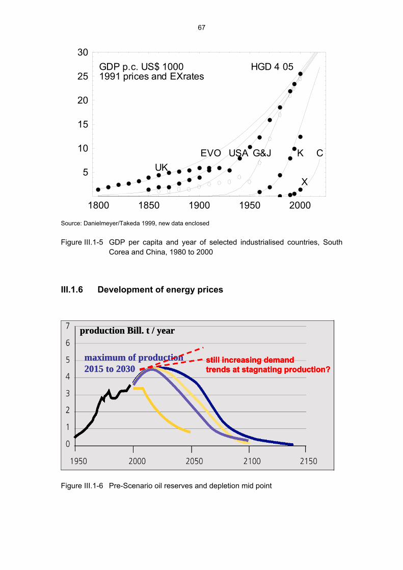
67

1800 1850 1900 1950 2000

5

10

15

20

25

30

UK

GDP p.c. US$ 10001991 prices and EXrates

HGD 4�05

USAEVO G&J K

X

C

Source: Danielmeyer/Takeda 1999, new data enclosed

Figure III.1-5 GDP per capita and year of selected industrialised countries, South Corea and China, 1980 to 2000

III.1.6 Development of energy prices

maximum of production 2015 to 2030

still increasing demandtrends at stagnating production?

production Bill. t / year

maximum of production 2015 to 2030

still increasing demandtrends at stagnating production?

production Bill. t / year

maximum of production 2015 to 2030

still increasing demandtrends at stagnating production?still increasing demandtrends at stagnating production?

production Bill. t / year

Figure III.1-6 Pre-Scenario oil reserves and depletion mid point

68

Table III.1-3 Pre-Scenarios oil prices (fob) 2035 in $ per barrel

base price/ max. production year/ price increaseoil price (fob)

High: 35 $ / 2015 / 2,5 %/a 58

Quite high: 35 $ / 2020 / 2,5 %/a 51

Medium: 35 $ / 2020 /2,2 %/a 49

A bit low : 30 $ / 2020 / 2,0 %/a 41

Low : 30 $ / 2025 / 2,0 %/a 37

Table III.1-4 Price development of heating oil EL – Reference Scenario CH

2003 2005 2010 2015 2020 2025 2030 2035Rohöl FOB US$/Barrel 29.2 30.0 30.0 30.0 30.0 30.0 30.0 33.4Rohöl FOB CHF/1000 ltr. 248 255 255 255 255 255 255 294Rohöl CIF CHF/1000 ltr. 268 275 275 275 275 275 275 314

Netto-Großhändlerpreis CHF/1000 ltr. 352 359 359 358 357 356 355 394 excise tax CHF/1000 ltr. 3.55 3.55 3.55 3.55 3.55 3.55 3.55 3.55 emergency tax CHF/1000 ltr. 6.16 4.27 4.27 4.27 4.27 4.27 4.27 4.27 CO2-Tax (35 CHF/t CO2) CHF/1000 ltr. 95 95 95 95 95 95Brutto-Großhändlerpreis CHF/1000 ltr. 362 367 462 461 460 459 458 497

Netto-priv. HH-Preis CHF/1000 ltr. 408 413 508 507 506 505 504 543 excise tax CHF/1000 ltr. 9 9 9 9 9 9 9 9 emergency tax CHF/1000 ltr. 6.16 4.27 4.27 4.27 4.27 4.27 4.27 4.27 CO2-Tax (35 CHF/t CO2) CHF/1000 ltr. 95 95 95 95 95 95Zwischensumme 423 426 616 615 614 613 612 651MWSt (7,6/9,1(2010)/10,1(2015)/11(2020) 32 32 47 47 47 47 47 49Brutto-priv. HH-Preis CHF/1000 ltr. 449 454 563 562 561 560 559 602

69

Table III.1-5 Price development of natural gas - Scenario High, Switzerland

2003 2005 2010 2015 2020 2025 2035Import Rp/kWh (Untere Variante) 1.6 1.9 1.9 1.9 2.2 2.5 3.2

Industrie [Rp/kWh] Einkauf** 3.68 3.98 3.98 3.98 4.28 4.58 5.28 excise tax [Rp/kWh]*** 0.0146 0.0146 0.0146 0.0146 0.0146 0.0146 0.0146 emergency tax [Rp/kWh]*** 0.0200 0.0200 0.0200 0.0200 0.0200 0.0200 0.0200 CO2-Tax (35 CHF/t CO2) [Rp/kWh] 0.693 0.693 0.693 0.693 0.693Industrie [Rp/kWh] Verkauf** 3.72 4.01 4.71 4.71 5.01 5.31 6.01

private Haushalte Netto 6.03 6.33 6.33 6.33 6.63 6.93 7.63 excise tax [Rp/kWh]*** 0.0146 0.0146 0.0146 0.0146 0.0146 0.0146 0.0146 emergency tax [Rp/kWh]*** 0.0200 0.0200 0.0200 0.0200 0.0200 0.0200 0.0200 CO2-Tax (35 CHF/t CO2) [Rp/kWh] 0.693 0.693 0.693 0.693 0.693Zwischensumme 6.07 6.36 7.06 7.06 7.36 7.66 8.36MWSt (7,6/9,1(2010)/10,1(2015)/11(2020) 0.46 0.48 0.54 0.54 0.56 0.58 0.64private Haushalte Brutto (Rp/kWh) 6.49 6.81 6.87 6.87 7.19 7.51 8.27

Table III.1-6 Impact of projected climate change on electricity demand in the final energy sectors, in 2035, Reference Scenario

GWh / a Referenz zusätzlicher eingesparte Netto- ohne Klimaveränderung Kühlbedarf Raumwärme Effekte private Haushalte 20'722 3'055 355 16% Dienstleistungssektoren und Landwirtschaft 20'660 2'000 k. A.. 10%

Industrie und Baugewerbe 20'672 165 - 1% Transport 2'833 k. A. k. A. k. A..

[Lecture 6, 26. Apr. 2007]

70

Pre-Scenarios oil prices (fob) 2035 in $ per barrel

base price/ max. production year/ price increaseoil price (fob)

High: 35 $ / 2015 / 2,5 %/a : 58

Quite high: 35 $ / 2020 / 2,5 %/a : 51

Medium: 35 $ / 2020 / 2,2 %/a : 49

A bit low: 30 $ / 2020 / 2,0 %/a : 41

Low: 30 $ / 2025 / 2,0 %/a : 37

Figure III.1-7

Source: Prognos AG

Figure III.1-8

III.1.7 Conclusions on energy determining drivers

• Physical drivers – nice to have:

71

- floor area, number of households, number and age of electric appliances, number and capacities of boilers, air conditioners

• Economic boundary conditions important

- income of private households, energy prices and expectations

• Technologies and their efficiencies: influencial, but often not data

• Decision making of investors and behaviour of users extremely influencial (preferences, traditions, convenience, prestige) (no data available in most cases)

• Aggregated indicators as drivers as an often used solution e.g. personkm, net value added, floor area of office buildings

• the other solution for projections: specific energy use data

III.2. Energy services and energy demand projections

Transformation moduleE. Jochem (EJ)

Primary Energy

ConversionF. Noembrini

Co-generationF. Noembrini

Conversion Sectors etc.

Boundary Conditions – Data from the Database

Energy-efficientBoundary Conditions

Macro-modelM. Wickart (MW)

Energy sectorsHousehold &

Electrical appliances (GC)

ServicesG. Catenazzi

Industry E. Jochem

TransportationF. Noembrini (FN)

Cost moduleM. Wickart

Emissions

Modified Input, etc.

ConversionF. Noembrini

Co-generationF. Noembrini

Scenario-drivers and

Scenario variants

Sensitivity analyses of technical coefficients and cost

Transformation moduleE. Jochem (EJ)

Primary Energy

ConversionF. Noembrini

Co-generationF. Noembrini

Conversion Sectors etc.

Boundary Conditions – Data from the Database

Energy-efficientBoundary Conditions

Macro-modelM. Wickart (MW)

Energy sectorsHousehold &

Electrical appliances (GC)

ServicesG. Catenazzi

Industry E. Jochem

TransportationF. Noembrini (FN)

Cost moduleM. Wickart

Emissions

Modified Input, etc.

ConversionF. Noembrini

Co-generationF. Noembrini

Scenario-drivers and

Scenario variants

Sensitivity analyses of technical coefficients and cost

Figure III.2-1 Preferred areas of scenario-drivers, scenario variants and sensitivity analyses

72

Model of the technology cycle (scheme)

Breite Aktivitäten/

Möglichkeiten

ZeitEuphorie

Ernüch-terung Aufstieg

Ent-deck-ung

DiffusionNeu-

orient.

Aktivitätsniveau

1

2 34

5

6

New technologies: always quite costly

Figure III.2-2 Model of the technology cycle (scheme)

Co-operation / stock sharingseveral stacks deliveredDelivery contracts

Fuel cell manufacturers and users (car-industry – examples) as result of a patent- und co-operation analysis

ToyotaGM/Opel

Daihatsu

Hyundai

UTC

BMW

Nissan Renault PSA

Nuvera

Delphi

Volvo

VW

Mitsubishi

EvoBus

Isrisbus

Fiat

CelanesePlugPower

Ballard

Mazda

Honda

Ford

DC

Figure III.2-3

73

Table III.2-1 Combination of policy and supply variants

Source: Prognos AG

Figure III.2-4 Demand on Swiss final energy in Scenario I, in PJ, Trend – stagnation at around 800 PJ

74

Source: Perspektiven, Synthesebericht 2007

Figure III.2-5 2000 Watt per capita society in Switzerland: lowering the primary en-ergy demand per capita to 2000 W until 2100

Table III.2-2 CO2 emissions in scenario IV of electricity supply variants in mill. tons and changes in percent, base case boundary conditions

75

Figure III.2-6 Final energy and electricity demand per scenario, in PJ, in four scenar-ios (trend boundary conditions)

III.3. Cost of energy conversion and end-use technologies

76

Experience curves of several energy converters

1990

2000

1981

1985PV

(1981-2000)PR = 77%

1995

1985

2000

1981 1990

Wind (1985-2000)

PR= 88%

1981

1989

1995

CCGT(1989-1995)

PR = 81%

2000

19851980

2002

Ethanol (1980-1985)

PR = 93% 1990

100

1000

10000

100000

1 10 100 1000 10000 100000 1000000

Cumulative Installed Capacity in MW (PV, Wind, Gas Turbines)

101 100 1000 10000 100000 1000000

1

10

100

1000

Ethanol (1985-2002)

PR = 71%

Wind (1981-1985)PR = 99%

CCGT(1981-1989)PR = 104%

Cumulative ethanol volume (1000m3)

Figure III.3-1

Learning Curves – Overview

Unit cost reduction as a function of cumulative production or installed capacity:

Progress ratio (pr), learning rate (lr = 1–pr)

Estimates sensitive to model specification and estimation technique (e.g. Söderholm/Sundqvist 2004)

Many empirical LC studies on RETs (e.g. Neij 1997/99; Ibenholt 2002; Kamp et al. 2004)

1 2

1

( ) ( ) 1 2 1( )

bC C U M C C U M P RC C U M

−= − = −

77

Decreasing cost by learning and economies of scale of energy converting and efficiency investments

MARKALEurope

MARKALglobal

ReducedMARKAL global

ERISglobal

Advanced coal 0.94 0.93 0.95

Gas combined cycle 0.89 0.85 0.88

New nuclear 0.96 0.93

Fuel cell 0.82 0.87 0.82

Wind power 0.90 0.89 0.85 0.88

Solar pv 0.81 0.81 0.72 0.85

Solar thermal 0.85

Double glazing 1970-2000 0.85 – 0.9

Tripple glazingca Mid 1990s 0.85 – 0.9newSource: surveys and calculations CEPE

Quelle: Seebregts et al, 1999

Bisher nurfür Energie-wandler:

0,00

2,00

4,00

6,00

8,00

10,00

12,00

14,00

Wind on

shore

Wind of

fshore

Gas G

uD

Gas G

T

Steink

ohle

Braunk

ohle

Kernen

ergie

Erz

eugu

ngsk

oste

n [C

ent/k

Wh]

Kapitalkosten (2000h)Kapitalkosten (5000h)Kapitalkosten (7000h)Brennstoff + O&M Kosten

3800 h

2100 h

assumptions:- 20 years depreciation- 8 % interest rate

-15,5 – 16 €/MWh gas price- 5,7 €/MWh coal price0,00

2,00

4,00

6,00

8,00

10,00

12,00

14,00

Wind on

shore

Wind of

fshore

Gas G

uD

Gas G

T

Steink

ohle

Braunk

ohle

Kernen

ergie

Erz

eugu

ngsk

oste

n [C

ent/k

Wh]

Kapitalkosten (2000h)Kapitalkosten (5000h)Kapitalkosten (7000h)Brennstoff + O&M Kosten

3800 h

2100 h

assumptions:- 20 years depreciation- 8 % interest rate

-15,5 – 16 €/MWh gas price- 5,7 €/MWh coal price

Figure III.3-2

78

0,00

2,00

4,00

6,00

8,00

10,00

12,00

14,00

Wind

onsh

ore

Wind

offsho

re

Gas G

uD

Gas G

T

Steink

ohle

Braunk

ohle

Kernen

ergie

Erz

eugu

ngsk

oste

n [C

ent/k

Wh

Kapitalkosten (2000h)Kapitalkosten (5000h)Kapitalkosten (7000h)CO2-Kosten (30€/t)erhöhte BrennstoffkostenBrennstoff + O&M Kosten

assumptions:- 20 years depreciation- 8 % interest rate- 19 – 20 €/MWh gas price- 5,7 €/MWh coal price

0,00

2,00

4,00

6,00

8,00

10,00

12,00

14,00

Wind

onsh

ore

Wind

offsho

re

Gas G

uD

Gas G

T

Steink

ohle

Braunk

ohle

Kernen

ergie

Erz

eugu

ngsk

oste

n [C

ent/k

Wh

Kapitalkosten (2000h)Kapitalkosten (5000h)Kapitalkosten (7000h)CO2-Kosten (30€/t)erhöhte BrennstoffkostenBrennstoff + O&M Kosten

assumptions:- 20 years depreciation- 8 % interest rate- 19 – 20 €/MWh gas price- 5,7 €/MWh coal price

Figure III.3-3

0,00

2,00

4,00

6,00

8,00

10,00

12,00

14,00

Wind

onsh

ore

Wind

offsho

re

Gas G

uD

Gas G

T

Steink

ohle

Braunk

ohle

Kernen

ergie

Erz

eugu

ngsk

oste

n [C

ent/k

Wh

Kapitalkosten (2000h)Kapitalkosten (5000h)Kapitalkosten (7000h)CO2-Kosten (30€/t)erhöhte BrennstoffkostenBrennstoff + O&M Kosten

assumptions:- 20 years depreciation- 8 % interest rate- 19 – 20 €/MWh gas price- 5,7 €/MWh coal price

without externaleffects (air pollution, noise, climate change)

0,00

2,00

4,00

6,00

8,00

10,00

12,00

14,00

Wind

onsh

ore

Wind

offsho

re

Gas G

uD

Gas G

T

Steink

ohle

Braunk

ohle

Kernen

ergie

Erz

eugu

ngsk

oste

n [C

ent/k

Wh

Kapitalkosten (2000h)Kapitalkosten (5000h)Kapitalkosten (7000h)CO2-Kosten (30€/t)erhöhte BrennstoffkostenBrennstoff + O&M Kosten

assumptions:- 20 years depreciation- 8 % interest rate- 19 – 20 €/MWh gas price- 5,7 €/MWh coal price

without externaleffects (air pollution, noise, climate change)

Figure III.3-4

79

Figure III.3-5 Share of the yearly efficiency investments in scenario III and IV per GDP in %, including and excluding avoided energy imports

80

Figure III.3-6 Capital cost, energy cost savings and resulting net savings based on investments in Scenario III und IV, in Bill. CHF

III.4. External cost of energy use and their internalisation

81

Table III.4-1

yes (rivalrous) no (nondepletable)ye

spure private goods: e.g. electricity, bread, shoes, houses

natural monopol: e.g. coded television, patented knowledge, "italian" roadways

no

common property or open access resources, "Allmende" goods: e.g. ground water resources, natural environment

pure public goods: clean air, scenic views, knowledge, national defense, public lighting, roadways, avalanche protection

Excl

usivi

tyDivisibility (rivalness in consumption)

Electricity demand curve

Electricity price

Market price without CO2carge

Quantity of electricity produced by fossil fuel based power plants without CO2-emission certificates

*) corrosion of cars, fences, bridges;loss of agricultural production;respiratory illness (4 bill. CHF/a)

S = Supply curve marginal private costs of generation

External cost 0.1 to 2 cts/kWh*)

S1 = marginal social costs of generation

Def.: social cost = private cost + external cost

Electricity demand curve

Electricity price

Market price without CO2carge

Quantity of electricity produced by fossil fuel based power plants without CO2-emission certificates

*) corrosion of cars, fences, bridges;loss of agricultural production;respiratory illness (4 bill. CHF/a)

S = Supply curve marginal private costs of generation

External cost 0.1 to 2 cts/kWh*)

S1 = marginal social costs of generation

Def.: social cost = private cost + external cost

Figure III.4-1

[Lecture 8]

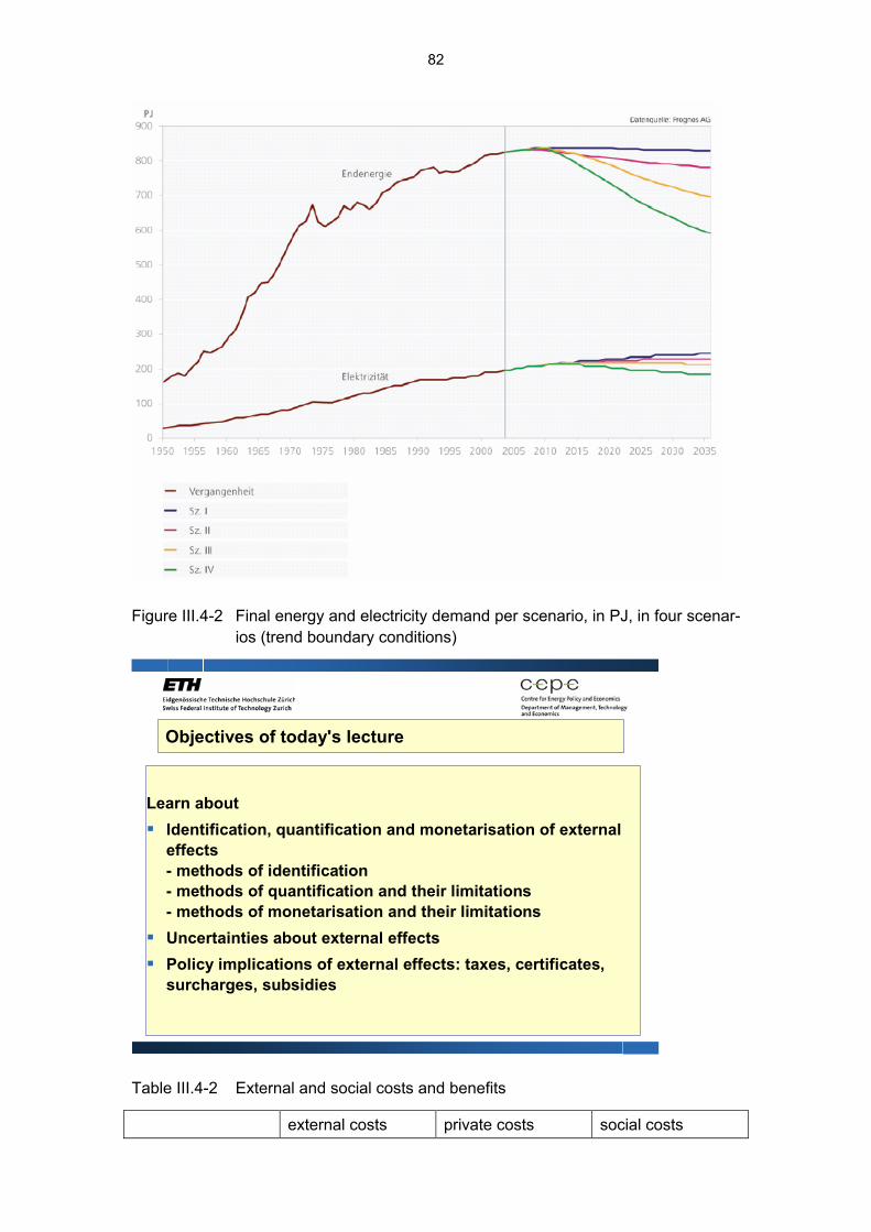
82

Figure III.4-2 Final energy and electricity demand per scenario, in PJ, in four scenar-ios (trend boundary conditions)

Objectives of today's lecture

Learn about Identification, quantification and monetarisation of external effects- methods of identification- methods of quantification and their limitations- methods of monetarisation and their limitationsUncertainties about external effectsPolicy implications of external effects: taxes, certificates, surcharges, subsidies

Table III.4-2 External and social costs and benefits

external costs private costs social costs

83

benefits beneficiary does not pay

beneficiary pays total of both

costs loser is not com-pensated

loser is compen-sated

total of both

Integrating external effects into the economic evaluation

Transformation moduleE. Jochem (EJ)

Primary Energy

ConversionF. Noembrini

Co-generationF. Noembrini

Conversion Sectors etc.

Boundary Conditions – Data from the Database

Energy-efficientBoundary

Conditions

Macro-modelM. Wickart (MW)

Energy sectorsHousehold &

Electrical appliances G.

Catenazzi (GC)

ServicesG. Catenazzi

Industry E. Jochem

TransportationF. Noembrini (FN)

Cost moduleM. Wickart

Emissions

Modified Input, etc.

ConversionF. Noembrini

Co-generationF. Noembrini

Scenario-drivers and

Scenario variants

Sensitivity analyses of technical coefficients and cost

Surcharges, taxes, subsidies

Identification of External Effects of Energy Use

External cost identification along chains of impactEnvironmental damages: allergies? breeds of trouts die? Reduced biodiversity?

Impact on social systems: more mobility, more road accidents, more cost for hospitals and rehabilitation, higher health insurance cost

economic impacts: depletion of non-renewable resources

External co-benefit identification along chains of impactenvironmental benefits: oxygen input into rivers by ship propulsion

societal benefits: additional net employment due to improved energy efficiency, additional exports of energy-efficient products

84

Emission(e.g. noise, electrosmog, visual pollution)

Dispersion(e.g. perception zone)

Impact(e.g. lower house prices)

Cost(e.g.value loss due to noise) Evaluation of the value loss due to

the burdens (monetarisation). All cost are summed over all receptors that may be affected by this burdens.

Evaluation of incremental pollutant concentrations (e.g. region affected by noise) in all affected regions.

perceived pollution

pric

e

demand curve

Characterisation of the relevant technologies and the environmental burdens they impose.

Characterisation of the population or receptor exposed to incremental pollution; identification of suitable exposure-response functions: demand curve; estitimation of social impact.

Demand-curve approaches: cost=f(perceived damage)

GIS

Emission(e.g. noise, electrosmog, visual pollution)

Dispersion(e.g. perception zone)

Impact(e.g. lower house prices)

Cost(e.g.value loss due to noise) Evaluation of the value loss due to

the burdens (monetarisation). All cost are summed over all receptors that may be affected by this burdens.

Evaluation of incremental pollutant concentrations (e.g. region affected by noise) in all affected regions.

perceived pollution

pric

e

demand curve

perceived pollution

pric

e

demand curve

Characterisation of the relevant technologies and the environmental burdens they impose.

Characterisation of the population or receptor exposed to incremental pollution; identification of suitable exposure-response functions: demand curve; estitimation of social impact.

Demand-curve approaches: cost=f(perceived damage)

GIS

Figure III.4-3 Following the impact pathways

Brain-Writing (using life cycle analysis) of external effects of using heating oil

and production

oil transport

refinery

heating oil distribution

heating oil use in buildings

individualsgroupseconomytechnical systemsphysical systems

Impacts on

85

Emission(e.g. kg/yr of particulates)

Dispersion(e.g. atmospheric dispersion model)

Impact(e.g. cases of illness due to particulates)

Cost(e.g. of illness due to particulates)

Economic valuation (monetarisation) of the impacts. All cost are summed over all receptors (population, crops, buildings, etc.) that may be affected by this burdens. [… cost of life, man-day lost, …]

Evaluation of incremental pollutant concentrations (e.g. mg/m3 of particulates) in all affected regions.

concentration

impa

ct dose response function

N

S

EW

Characterisation of the relevant technologies and the environmental burdens they impose.

Characterisation of the population or receptor exposed to incremental pollution; identification of suitable exposure-response functions; estimation of physical impact.

Not

pos

sibl

ebe

caus

eof

man

yre

ason

s

Emission(e.g. kg/yr of particulates)

Dispersion(e.g. atmospheric dispersion model)

Impact(e.g. cases of illness due to particulates)

Cost(e.g. of illness due to particulates)

Economic valuation (monetarisation) of the impacts. All cost are summed over all receptors (population, crops, buildings, etc.) that may be affected by this burdens. [… cost of life, man-day lost, …]

Evaluation of incremental pollutant concentrations (e.g. mg/m3 of particulates) in all affected regions.

concentration

impa

ct dose response function

concentration

impa

ct dose response function

N

S

EW

N

S

EW

N

S

EW

Characterisation of the relevant technologies and the environmental burdens they impose.

Characterisation of the population or receptor exposed to incremental pollution; identification of suitable exposure-response functions; estimation of physical impact.

Not

pos

sibl

ebe

caus

eof

man

yre

ason

s

Figure III.4-4 Impossible to follow the impact pathways

Problems of Quantifying External Effects Related to Energy Use

Quantification often not easy/very difficult and costly/impossible(?), due to:limited knowledge: unknown chains of quantitative impact, particularly ofbiological or economic causal relationshipsallocation problems: several environmental stresses (e.g. smoking, airquality in production facilities or indoor chemicals from furniture) cannot beseparatedmethod of measurement is not available or generally accepted (e.g.changes of a scenic view, destruction of a national park)uncertainties: long time horizon, ... ExternE: „... one of the most importantconclusions is that uncertainties are large.“

Direct monetarisation via WTP/WTA approaches are sometimes easier to realise than quantification of the effect via dose-response or other bottom-up quantification methods.

86

Travel cost method: Assumption, incurred costs of visiting a site reflect the “value” of that site (Questionnaires)

Non-demand curve approaches: dose-response, replacement cost, shadow project approach, mitigation behaviour, opportunity cost

Hedonic pricing method: Attempts to evaluate environmental services

Contingent valuation method: Asking individuals explicitly to place values upon environmental assets

Methods for the Monetarisation of Externalities

Travel Cost Method

(Demand curve approaches – revealed preference type of evaluation)The travel cost method (TCM) can be used to estimate demand curves (WTP) for recreation sites an thereby value those sites. The underlying assumption is a simply one, that the incurred costs of visiting a site (e.g.petrol costs) in some way reflect the recreational value of that site. Questionnaires are used to ask visitors to the recreational sites where they have travelled from. From visitors' responses, we can estimate their travel costs and relate this to the number of visits per year. Not surprisingly, this relationship generally shows a typical downward sloping demand curve relationship between the cost of a visit and the number of visits taken, i.e. people living a considerable distance form a recreational site (facing high travel costs) make few visits per year, while those living near the site (with low travel costs) tend to make more frequent visits.

Additional explanatory factors to be taken into account: income of visitors, number of alternative sites available to each visitor, their personal interest in the type of site, etc. A real life study will typically interview several hundred visitors.

[see also Turner et al., 1994]

87

Evaluation Problems

Identification problem ...Quantification problems: quantification is often noteasy/extremely difficult and costly/impossibleDiscount rate: Discounting is the practice of placing lowernumerical values on future costs and benefits compared tothose of the present. Is it „right“ to discount? What would bethe appropriate discount rate? (market discount rate vs.social discount rate vs. opportunity cost discount rate)Value system: intrinsic value, future generations values, ...Risk evaluation: risk = probability of occurrence *

consequence of accident; still appropriate for low-probability / high consequence risks?

0,00

2,00

4,00

6,00

8,00

10,00

12,00

14,00

Wind

onsh

ore

Wind

offsh

ore

Gas GuD

Gas G

T

Steinko

hle

Braunko

hle

Kernenerg

ie

Erz

eugu

ngsk

oste

n [C

ent/k

Wh

Kapitalkosten (2000h)Kapitalkosten (5000h)Kapitalkosten (7000h)CO2-Kosten (30€/t)erhöhte BrennstoffkostenBrennstoff + O&M Kosten

assumptions:- 20 years depreciation- 8 % interest rate- 19 – 20 €/MWh gas price- 5,7 €/MWh coal price

0,00

2,00

4,00

6,00

8,00

10,00

12,00

14,00

Wind

onsh

ore

Wind

offsh

ore

Gas GuD

Gas G

T

Steinko

hle

Braunko

hle

Kernenerg

ie

Erz

eugu

ngsk

oste

n [C

ent/k

Wh

Kapitalkosten (2000h)Kapitalkosten (5000h)Kapitalkosten (7000h)CO2-Kosten (30€/t)erhöhte BrennstoffkostenBrennstoff + O&M Kosten

assumptions:- 20 years depreciation- 8 % interest rate- 19 – 20 €/MWh gas price- 5,7 €/MWh coal price

Figure III.4-5 Power generating cost – fossil fuels (high gas price), coal, and nuclear, external effects included by CO2 emission certificates

88

Conclusions

External Effects (conventional pollution + adaptation + damage cost)

Impacts on society and individuals often not identified- knowledge in social sciences less developed (complexity)

- impacts are third/fourth order effects (other influences)

- influences by stakeholders and media

Uncertainties of impacts in complex systems (observation process)

Unidentified effects cannot be managed at all

External effects justify subsidies in non-polluting options or taxes

III.5. Energy demand and supply projections and the limits of present energy models

• macro-economic energy models, technological progress and complete causal relationships of an economy (top down models)

• process-oriented energy models, technical detail, but partial causal relation-ships (bottom up models)

• building the bridge by integration the two model types into one system by soft or hard links

89

Übersicht zur Vorlesung Energiewirtschaft und EnergiepolitikEnergiestatistik

- beschreibende- analytische- DatenquellenEnergieressourcen

- Reserven- Ressourcen

Rationelle Energieanwendung

- Effizienzpotentiale- Energiedienstleistungen

Energiepolitik

- Maßnahmen und Bündel- EU und international

Hemmnisse undMarktunvollkommenheiten

- allgemeine Defizite- sektorale Hemmnisse

Energieperspektiven

- Szenariotechnik- Modellierung

Unternehmen und Märkte- Produktionskosten und Preise- Externe Kosten- Deregulierung der Märkte

Energienachfrage

- mikroökonomische Analysen I und II

Energietechnik

Wärmetechnik

Elektrotechnik

Bautechnik

today

Figure III.5-1 Overview

III.5.1 Objectives of the top down models and the bottom up models

Objectives of top down (macro-economic) energy models

• Simulate the drivers and the impacts of energy demand and supply of a coun-try within the next two or three decades, including energy price effects on all energy consumers

• Major design assumption: the economy is in equilibrium, policy intervention leads usually to higher societal cost that have to be identified and minimized

Objectives of bottom up models

• Simulate the energy demand and supply of a country within the next two or three decades in a technical detail appropriate to understand the technologi-cal changes of the energy system including their cost and emissions

• Major design assumption: the energy system can change in its technological structure without substantially effecting the economy

90

Transformation moduleE. Jochem (EJ)

Primary Energy

ConversionF. Noembrini

Co-generationF. Noembrini

Conversion Sectors etc.

Boundary Conditions – Data from the Database

Boundary Conditions

Macro-modelM. Wickart (MW)

Energy sectorsHousehold &

Electrical appliances G.

Catenazzi (GC)

ServicesG. Catenazzi

Industry E. Jochem

TransportationF. Noembrini (FN)

Cost moduleM. Wickart

Emissions

Modified Input, etc.

ConversionF. Noembrini

Co-generationF. Noembrini

The usual situation:-Macro modellers use "their" models

- bottum up modellers use "theirs"

- the results differ greatly

Transformation moduleE. Jochem (EJ)

Primary Energy

ConversionF. Noembrini

Co-generationF. Noembrini

Conversion Sectors etc.

Boundary Conditions – Data from the Database

Boundary Conditions

Macro-modelM. Wickart (MW)

Energy sectorsHousehold &

Electrical appliances G.

Catenazzi (GC)

ServicesG. Catenazzi

Industry E. Jochem

TransportationF. Noembrini (FN)

Cost moduleM. Wickart

Emissions

Modified Input, etc.

ConversionF. Noembrini

Co-generationF. Noembrini

The usual situation:-Macro modellers use "their" models

- bottum up modellers use "theirs"

- the results differ greatly

Figure III.5-2 Energy Navigator Switzerland defining the boundary conditions

Macro economic energy models and their characteristics

• Models describe the whole domestic economy by either a general equilibrium model or an econometric model:

- flow of goods, services, and capital as well as labour

- prices of the goods, services, capital and labour

- other input than capital and labour is energy

- improvement of energy efficiency is simulated by fixed productivity increases over time and by energy price-induced technical change of large sectors; no new technical innovation occur (or cannot be made explicit)

• Policy measures are mainly restricted to price policies (influencing the price-induced technological progress or energy substitution)

• The advantage: the effects of changed energy demand and supply on capital, labour, their prices, or economic growth can be evaluated

91

Market forproductioninputs , e.g.

labour, capital

Marketfor goods

and services

Money

Goods

e.g.

labo

ur

e.g. salaries , wages

e.g. subsidies

e.g. taxes

e.g. social securitybenefits

e.g. taxes

Companies

Public authorityat federal,

regional andlocal level

PrivateHous eholds

Natural resources

Natural environment Natural

environment

foreign producers foreign consumers

Market forproductioninputs , e.g.

labour, capital

Marketfor goods

and services

Money

Goods

e.g.

labo

ur

e.g. salaries , wages

e.g. subsidies

e.g. taxes

e.g. social securitybenefits

e.g. taxes

Companies

Public authorityat federal,

regional andlocal level

PrivateHous eholds

Natural resources

Natural environment Natural

environment

Market forproductioninputs , e.g.

labour, capital

Marketfor goods

and services

Money

Goods

Money

Goods

e.g.

labo

ur

e.g. salaries , wages

e.g. subsidies

e.g. taxes

e.g. social securitybenefits

e.g. taxes

Companies

Public authorityat federal,

regional andlocal level

PrivateHous eholds

Natural resources

Natural environment Natural

environment

foreign producers foreign consumers

Figure III.5-3 Cycle of money and goods and services in an economy a macro-model scheme

Functions and scheme of a macro-economic model

Typical functions:

• production functions = f (input of capital, labour, energy, time dependent technical progress)

• cost functions = f (input prices of capital, labour and energy, time and price dependent technical progress)

• consumption functions = f (income, product characteristics and prices)

• balancing functions: total tax income, subsidies, state investments and own operating cost, interest payments (for public au-thorities)

= total wages, total capital income by private households, total expenditures, interest payments, taxes (for private households)

• Exports and imports get specific attention in balancing flows of goods and payments

Questions difficult to be answered by macro-economic models

92

• Future structural changes in industry due to technological changes (e.g. less energy-intensive production due to more material efficiency)

• Identification of the impact of energy price changes on new energy technol-ogy options (back stop technologies) and related changes in energy demand (future changes in price and demand elasticities)

• Quantification of the impact of technical standards (efficiency, substitution) on energy demand and energy supply

• Similar problems regarding informational instruments (e. g. professional train-ing, learning local networks, initial consulting) and other instruments of entre-preneurial innovations (e.g car pooling, renting of construction machinery) when empirical data are available

Bottom up energy models and their characteristics

Models describe the energy using and converting system of an economy by either a simulation or an optimisation model:

• flow of different energy carriers in the final energy and conversion sectors

• technical parameters like conversion efficiencies, shares of different

• processes, cohorts of energy using appliances by classes of years

• emissions of air pollutants, climate gases, wastes

• economic or technical restrictions e.g. re-investment cycles, minimum domes-tic energy supply,

• cost of the various technologies (often in additional cost values which means to rely on a reference scenario), cost reduction by experience

• optimisation models produce shadow prices, the cost of technical options

• no feed back to macro economic aspects e.g. reduced/increased demand of goods due to increased (or reduced) energy cost/prices

93

Typical equation for energy demand E

E = Σ (drivers • specific energy)

• Partial sectoral models

• no feed back loops to macro-economic aspects

Quantities (e.g. heated, ventilated,

lighted floor area)

Typical equation for energy demand E

E = Σ (drivers • specific energy)

• Partial sectoral models

• no feed back loops to macro-economic aspects

Quantities (e.g. heated, ventilated,

lighted floor area)

Figure III.5-4 Typical structure of a process-oriented energy model for the industrial or service sector

Typical equation for energy demand E

E = Σ f(drivers • specific energy use; cost) if demand of drivers is satisfied and cost minimised

• Partial sectoral models• no feed back loops to

macro-economic models

Typical equation for energy demand E

E = Σ f(drivers • specific energy use; cost) if demand of drivers is satisfied and cost minimised

• Partial sectoral models• no feed back loops to

macro-economic models

Figure III.5-5 Example of an optimisation model of the basic chemical industry minimising the production cost of a given set of quantities of basic chemicals

Questions difficult to be answered by bottom up models

• Future demand of energy-intensive product due to inconsistent assumptions that the demand will not change although more steel, non-ferrous metals, insula-tion materials, glass are needed for the policy scenario

94

• The impact of changes in energy prices or cost of energy services on final demand is unclear

• The impact in suggested financial programmes and subsidies on the public households, on prices and employment is unclear

• Quantification of the impact on export and imports of products and services is unclear

• In many cases: iterative calculations of macro and bottom up model would be needed

The solution: linking macro-economic and bottom up energy models

• Each type of models has its own advantages and draw backs; one will not fix it in their own type of model design

• Advantages and draw backs are complementary; why not trying to combine the models by soft or hard links?

- get the technological details from the bottom up models as well as their abil-ity to model sectoral non-financial policies and the additional cost of effi-ciency and energy substitution

- get the comprehensive picture of the economy, the impact on changing final demand and investments, on prices and employment, on economic growth and changing exports/imports and taxes

Not an easy task, but manageable by teams experienced in both fields of energy modeling, the present research frontier at ETH/CEPE

95

Transformation moduleE. Jochem (EJ)

Primary Energy

ConversionF. Noembrini

Co-generationF. Noembrini

Conversion Sectors etc.

Boundary Conditions – Data from the Database

Boundary Conditions

Macro-modelM. Wickart (MW)

Energy sectorsHousehold &

Electrical appliances G.

Catenazzi (GC)

ServicesG. Catenazzi

Industry E. Jochem

TransportationF. Noembrini (FN)

Cost moduleM. Wickart

Emissions

Modified Input, etc.

ConversionF. Noembrini

Co-generationF. Noembrini

The future situation:-Macro modellers deliver to transformation module

- bottum up modellers deliver to macro models

- consistent results to be expected

Transformation moduleE. Jochem (EJ)

Primary Energy

ConversionF. Noembrini

Co-generationF. Noembrini

Conversion Sectors etc.

Boundary Conditions – Data from the Database

Boundary Conditions

Macro-modelM. Wickart (MW)

Energy sectorsHousehold &

Electrical appliances G.

Catenazzi (GC)

ServicesG. Catenazzi

Industry E. Jochem

TransportationF. Noembrini (FN)

Cost moduleM. Wickart

Emissions

Modified Input, etc.

ConversionF. Noembrini

Co-generationF. Noembrini

The future situation:-Macro modellers deliver to transformation module

- bottum up modellers deliver to macro models

- consistent results to be expected

Figure III.5-6 The solution: linking macro-economic and bottom up energy models

Central tasks for linking the top down and bottom up models

• Translation of energy demand related information of the macro economic models into energy drivers - Transformation Module:

- gross production of the construction materials industry to cement, lime, bricks, ceramics, glass

- developing independently a view on future material efficiency reducing the demand of construction material

- calculating floor area of homes and office buildings from macro data

• Translation of the individual investments in energy sectors (and related policies) into data relevant for the macro model, e.g.:

- total additional investment by mechanical and electric engineering sectors

- total changes in turnover of the electricity, gas, or mineral oil industry

- change in the energy consumption structure of industries, services etc.

Hints for literature

Special Issue of the Energy Journal, April 2006 ("Endogenous Technological Change and the Economics of Atmospheric Stabilisation")

96

For the interested reader:

Popp, D. (2006). ENTICE-BR: The effects of backstop technology R&D on climate

policy models. Energy Economics 28 (2006) 188-222

[Lecture 9]

Models for projecting future energy demand and supply

Objectives

Why modelling energy demand and supply of the future ?What type of models do we have available?How to analyse the risks and benefits of over and under investments in energy supply

Learning methodological approachesBottom up modelsMacro-economic modelsHybrid modelsMulti agent models

The task: Projecting the Energy-Flow of Switzerland 2002 into the future

Space Heat 225 76,4

Process Heat 82,0 55,6Motive Powert

Other Drives 52,8 60,6

Illumination 21 8,5

Information, n.d. n.d.Communication

55,7 20,0

Nutzenergie der Endenergiesektoren

21,3 PJ non-energetic Consumption

Final Energy853,7 PJ

Primary energy1.147 PJ

Industry 168,5 PJTransportation 302,8 PJ

Private Households 230,6 PJ

Trade, Commerce, 153,5 PJ

271,8 PJ

Transformation Losses

Energy Services

Heated Rooms(in qm)

Industrial Products(in tons)Mobility(in Pass.km)Automation,CoolingIlluminated Areas(in qm)PC-, Phone- and Internet Use

2

Losses for generatingUseful EnergyUseful Energy

(Incl. 23 PJ Distribution Losses)

PJ

Source: ISI, Karlsruhe

Nutzungs-grad in %

429 PJ 425 PJ

Plastics,Asphalt

K:\E\Daba-al\Energieflussdiagramme\2002_en-Energiefluss Schweiz\2002Energiefluss Folie.ppt

24,1%38,1% 37,8 %

97

Energy Navigator Switzerland defining the boundary conditions

Transformation moduleE. Jochem (EJ)

Primary Energy

ConversionF. Noembrini

Co-generationF. Noembrini

Conversion Sectors etc.

Boundary Conditions – Data from the Database

Energy-efficientBoundary

Conditions

Macro-modelM. Wickart (MW)

Energy sectorsHousehold &

Electrical appliances G.

Catenazzi (GC)

ServicesG. Catenazzi

Industry E. Jochem

TransportationF. Noembrini (FN)

Cost moduleM. Wickart

Emissions

Modified Input, etc.

ConversionF. Noembrini

Co-generationF. Noembrini

The first step:- From pre-scenarios to- full consistant, plausiblescenarios

Questions of the OFE (Bundesamt für Energie) –How does the Swiss energy system evolve during the next 30 years?

What are the major drivers for more or less energy demand in thevarious sectors of final energy and energy conversion?

Can they be influenced by political or innovative measures and activities?

How material demand can be reduced? And how the demand of useful energy of buildings, vehicles, industrial processes?

How can efficiencies of energy conversion be improved?

How much does it cost compared to do no specific activities?

98

Typical equation for energy demand E

E = Σ (drivers • specific energy use)

• Partial sectoral models

• no feed back loops to macro-economic models

Typical equation for energy demand E

E = Σ (drivers • specific energy use)

• Partial sectoral models

• no feed back loops to macro-economic models

Figure III.5-7 Typical structure of a process-oriented energy model for the industrial or service sector

Determination of the development of new dwellings – example for stepping down from the boundary conditions to energy drivers

Newdwelling0m = MFH,t = e2.652208*(Ln(1000*GDPt-5) - Ln(1000*GDPt-6)) –2.011428*(Ln(1000*GDPt-5) - Ln(1000*GDPt-6)) + 0.714005*Ln(AGE_25 t) – 0.967011*Ln(AGE75_85 t) + 0.346158*Ln(newdwelling1m=MFH, t-1) + 0.210489 * dwelinctiv t + 10.801886 for t=2002

As a function of GDP, population age structure, dwellings in cities, number of new dwellings of the last year

• the computed result is not necessarily valid although the quality measures of the statistics may suggest this; plausibility checks quite useful

99

BIP(400) / BIP(seco): -7.4271%

BIP(seco ref+0,5%) / BIP(seco ref):

15.8734%

BIP(800) / BIP(seco): 15.9144%

-20%

0%

20%

2009

2016

2023

2030

BIP(400) / BIP(seco) BIP(seco ref+0,5% p.a.) / BIP(seco ref) BIP(800) / BIP(seco)

High pre-scenario at 800 CHF/ cap . a

Low pre-scenario at 400 CHF/ cap . aBIP(400) / BIP(seco):

-7.4271%

BIP(seco ref+0,5%) / BIP(seco ref):

15.8734%

BIP(800) / BIP(seco): 15.9144%

-20%

0%

20%

2009

2016

2023

2030

BIP(400) / BIP(seco) BIP(seco ref+0,5% p.a.) / BIP(seco ref) BIP(800) / BIP(seco)

High pre-scenario at 800 CHF/ cap . a

Low pre-scenario at 400 CHF/ cap . a

Figure III.5-8 Percentage deviation of two alternative pre-scenarios "high" and "low" relative to trend development (seco Reference = zero % line) 2000 to 2035

Table III.5-1 Gross domestic product per capita and year, Switzerland past and future 1970-2003 and 2000-2020; quite optimistic by plausibility check

2010 – 20202437.5458'554 441.520202005 – 20156507.5256'117 422.020152000 – 20105087.4853'142 397.520101995 – 20055167.4149'609 367.620051990 – 20001277.2048'061 346.020001985 – 19952147.0844'647 316.119951980 – 19906126.8046'690 317.319901975 – 19855496.5342'506 277.719851970 – 19804526.3940'564 259.01980

6.4037'069 237.21975(CHF / capita / year)6.2736'039 225.91970

Per capita growth of GDPpopulation(Mio.)

GDP / cap(CHF)

GDP (Billion CHF,

1990)

2010 – 20202437.5458'554 441.520202005 – 20156507.5256'117 422.020152000 – 20105087.4853'142 397.520101995 – 20055167.4149'609 367.620051990 – 20001277.2048'061 346.020001985 – 19952147.0844'647 316.119951980 – 19906126.8046'690 317.319901975 – 19855496.5342'506 277.719851970 – 19804526.3940'564 259.01980

6.4037'069 237.21975(CHF / capita / year)6.2736'039 225.91970

Per capita growth of GDPpopulation(Mio.)

GDP / cap(CHF)

GDP (Billion CHF,

1990)

Sources: BFE 2003, BFS several years, own assumptions

100

1000 VZÄ

1'500

2'000

2'500

3'000

DL, Trend 2'202 2'287 2'330 2'340 2'314 2'275 2'265

DL, positive Dynamik 2'202 2'357 2'474 2'556 2'599 2'626 2'684

DL, negative Dynamik 2'202 2'252 2'260 2'235 2'175 2'105 2'061

2005 2010 2015 2020 2025 2030 2035

Figure III.5-9 From GDP to working people in the service sector and in agriculture 2005-2035 in three scenarios, the interim step to the floor area

0

10

20

30

40

50

60

70

80Energie-Bez ugs -Fläc he (EBF)

Mio. m²

Handel 18.3 19.9 21.0 22.1 23.3 24.5 25.5 26.3 26.9 27.4

Banken und V er f s ic herungen 6.7 7.3 7.3 7.2 7.3 7.5 7.6 7.6 7.7 7.6

Hotels und Gas ts tätten 11.4 11.6 11.6 11.8 12.1 12.5 12.9 13.2 13.5 13.7

Bildung 22.6 23.3 24.1 25.0 26.3 27.5 28.5 29.3 30.0 30.6

Ges undheits - und Soz ialw es en 14.8 15.6 16.5 17.7 18.9 20.0 21.0 21.8 22.5 23.1

A ndere Diens tle is tungen 45.2 50.1 53.0 56.5 60.1 63.8 67.0 69.7 72.0 74.1

Landw ir ts c haf t 6.1 6.3 6.4 6.4 6.5 6.6 6.7 6.8 6.9 6.9

1990 1995 2000 2005 2010 2015 2020 2025 2030 2035

Figure III.5-10 The energy driver: heated floor area of the service sectors and agricul-ture Switzerland, 1990 to 2000 and Reference-Scenario 2000 to 2035

Table III.5-2 Gross value added in the branches of Swiss industry and construction 1990 to 2000 and Reference Scenario (in Mio. CHF1990)

Wertschöpfung in den Industriebran-chen 1990 1995 2000 2005 2015 2025 2035

Nahrung 7'400 8'266 8'265 8'512 8'212 7'714 6'974

Bekleidung 2'847 2'222 1'687 1'729 1'979 2'097 2'117

Papierindustrie 1'393 1'521 1'607 1'632 1'750 1'776 1'747

101

Chemie 5'614 9'335 12'750 14'680 16'727 18'609 21'184

Glas 535 450 417 422 450 454 447

Keramik 535 450 417 422 450 454 447

Zement 161 135 125 127 135 136 134

NE-Mineralien 1'445 1'214 1'126 1'139 1'214 1'226 1'208

Metalle 1'030 1'024 1'065 1'126 1'217 1'236 1'208

NE-Metalle 515 512 533 563 609 618 604

Metallerzeugnisse 7'570 7'525 7'701 8'175 8'841 8'974 8'774

Maschinenbau 13'021 11'930 12'820 13'771 15'755 16'699 17'067

Elektrotechnik 13'621 14'749 15'384 16'719 18'967 20'064 20'473

Energie 7'463 9'728 8'981 9'381 9'894 10'000 9'868

Bau 26'797 24'063 21'285 22'013 24'389 25'440 26'061

Übrige 13'762 12'930 13'881 14'743 16'528 17'379 17'751

Industrie total 103'710 106'052 108'043 115'153 127'115 132'875 136'066

Technological trends as energy drivers for fuels and electricity

More electronics & informatics, additional automation in all sectors +/-

Microsystemstechnics (producing individually and without losses ) +/-

"cool" physico-chemical processes (e. g. membranes, biotechnology,

extraction, absorption, impulse drying, ….) - fuels / + electricity

New plastics with better properties or made out of biomass -

"Robotics" in all service branches and private households +

More technical equipment in private households and leisure +

102

Comparison of the projected electricity demand of the final energy sectors of three scenarios for 2035, Switzerland

GWh / a Referenz I

Perspektiven"Hoch"- Szenario

"Tief" - Szenario

Hoch/Ref Tief/Ref

private Haushalte 20'722 22'126 19'259 6.8% -7%

Industrie und Baugewerbe 20'662 23'555 19'112 14% -7.5%

Dienstleitungssektoren 17'371 20'320 15'770 17% -9.2%

Transport 2'833 3'050 2'750 7.6% -3.0%

Endenergie, total (gerundet) 61'590 69'050 56'890 12% -7.6%

• the highest deviations from the Reference Scenario in industry and the service sector

• an additional increase of electricity demand is expected by increasing temperatures due to climate change

• transport plays a minor role in electricity use, even less in the future

M:\C

EPE

Züric

h\V

orle

sung

\Lau

sann

e\SS

-200

3\Fo

lien\

Teil

2.pp

t

Cycle of money and goods in an economy

Market forproductioninputs, e.g.

labour, capital

Marketfor goods

and services

Money

Goods

e.g.

labo

ur

e.g. salaries, wages

e.g. subsidies

e.g. taxes

e.g. social securitybenefits

e.g. taxes

Companies

Public authorityat federal,

regional andlocal level

PrivateHouseholds

Natural resources

Natural environment Natural

environment

foreign producers foreign consumers

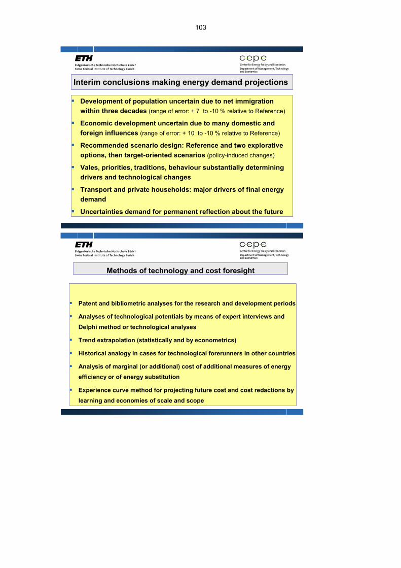
103

Interim conclusions making energy demand projections

Development of population uncertain due to net immigration within three decades (range of error: + 7 to -10 % relative to Reference)

Economic development uncertain due to many domestic and foreign influences (range of error: + 10 to -10 % relative to Reference)

Recommended scenario design: Reference and two explorative options, then target-oriented scenarios (policy-induced changes)

Vales, priorities, traditions, behaviour substantially determining drivers and technological changes

Transport and private households: major drivers of final energy demand

Uncertainties demand for permanent reflection about the future

Methods of technology and cost foresight

Patent and bibliometric analyses for the research and development periods

Analyses of technological potentials by means of expert interviews and

Delphi method or technological analyses

Trend extrapolation (statistically and by econometrics)

Historical analogy in cases for technological forerunners in other countries

Analysis of marginal (or additional) cost of additional measures of energy efficiency or of energy substitution

Experience curve method for projecting future cost and cost redactions by learning and economies of scale and scope

104

Hints and conclusions making energy projections

Explorative and conditioned kinds of projections (Scenarios) "Prognosis" in the sense "What will be?" is impossible in social systems

Reference scenario needed for quantifying the additional cost oftarget-oriented (policy driven) projections

Major technological influences: make them transparent and open to discussion

Possible development paths to be described by the documented relevant boundary conditions

Do not forget in economic analyses to include the macro-economic perspective (including external effects, partial models not sufficient for economic assessment))

105

Glossary This glossary should support the understanding of the English literature as well as to develop a joint understanding of the expert language of energy economics and policy. it is still under development and hints for improvement by the students are very wel-come. Ancillary benefits The ancillary, or side effects, of investments and policies aimed exclusively at climate change mitigation. Such policies have an impact not only on greenhouse gas emis-sions, but also on emissions of local and regional air pollutants associated with fossil fuels, and on issues such as transportation, agriculture, employment, and fuel secu-rity. Barrier A barrier is any obstacle to reaching an economic potential of resource efficiency that can be overcome by a policy, programme, or measure not only by government, but also by trade associates or other third parties (another term for barrier, often used, is obstacle). Co-benefits The benefits of investment and policies that are implemented for various reasons at the same time – including energy or material efficiency – acknowledging that most policies designed to address resource efficiency also have other, often at least equally important, rationales (e.g. related to objectives of improved product quality or capital and labour productivity). Co-generation The use of waste heat from electric generation, such as exhaust from gas turbines, for either industrial purposes or district heating. Contracting Contracting is the outsourcing of an energy converting plant (e.g. heat generation, co-generation, production of compressed air, cold, or technical gases) that is planned, built, financed, operated and maintained by an other company (energy service com-pany). It can also cover energy saving services such as efficient illumination, heat recovery and insulation of buildings (the latter facing legal obstacles). Economic Potential Economic potential is the portion of technological potential for energy or material effi-ciency improvements that could be achieved cost-effectively through the creation of markets, reduction of market failures, increased financial and technological transfers. The achievement of economic potential requires additional policies and measures to break down market barriers. Energy efficiency Ratio of energy output of a conversion process or of a system to its energy input or of an energy service to its useful energy input. Energy intensity Energy intensity is the ratio of energy use to economic or physical output. At the na-tional level, energy intensity is the ration of total domestic primary energy consump-tion on final energy consumption to Gross Domestic Product, value added, or physi-cal output such as heated floor area or person-km.

106

Energy service The application of useful energy to tasks desired by the consumer such as transpor-tation or persons and freight, a warm room, or illuminated production facility, or ton-nes of electro steel produced. Final energy Energy supplied that is available to the consumer to be converted into useful energy (e.g. electricity at the wall outlet, heating oil, gasoline, diesel, natural gas, coke, wood ships). Frozen efficiency The material or energy efficiency of today is projected to be the same in future years. Gross Domestic Product (GDP) The sum of all values added produced by all economic sectors of a national economy within a given period of time (e.g. during one year). Material efficiency Ratio of a desired service to the physical quantity of material necessary to deliver the service (e.g. 0.6 to 2.0 tonnes per car, 30 g per 1 ltr. glass bottle, 60 g per m2 news-paper). Mitigation An anthropogenic intervention to reduce the source or enhance the sinks of green-house gases (e.g. by energy and material efficiency, renewable energies instead of fossil fuels). Pooling Machines or vehicles are used by several customers instead of owning them. The renting or leasing is organised by a service organisation that generally owns and maintains the pool. Primary energy Energy embodied in natural resources (e.g. coal, crude oil, natural gas, sunlight, wood, wind, bio-mass, uranium) that has not undergone any anthropogenic conver-sion or transformation. Recycling The material of an used product or vehicle is returned to the production step of sec-ondary material after being shredded, selected and eventually purified (steel scrap for input into electric arc furnaces to produce new steel). Re-use An used product or vehicle is partially or totally returned to the market after some repairs, amelioration or partial substitution of components (e.g. tires, gear boxes, combustion engines, glass bottles, frame of copy machines). Structural change Changes over time in the relative shares of energy-intensive and-extensive economic sectors in the industrial, agricultural, or services sector, changes of the share of floor area of one- and two-family houses to the total floor area of residential buildings or of heavy, large cars of the car stock. Technical potential The amount by which it is possible to improve energy and material efficiency by im-plementing a technology or practice that has already been demonstrated.

107

Useful energy The energy use related to all energy losses that are lost by end-uses (heated rooms, moving vehicles) to dissipated heat at ambient temperature.

Status 24 May 2007