energy analysis and modelling: power sector modelling with ... · energy analysis and modelling:...
TRANSCRIPT
© OECD/IEA 2013
Energy Analysis and Modelling: Power Sector Modelling with TIMES
Energy Training Week 2014
8-9 April, 2014
Uwe Remme, Luis Munuera
© OECD/IEA 2013
Module overview
8 April: Power Sector Modelling with TIMES (1)
Introduction to energy systems modelling and TIMES
Getting started in running a power sector model in TIMES (using
ANSWER-TIMES and a simplified Excel interface)
9 April: Power Sector Modelling with TIMES (2)
Refining the power sector analysis:
Treatment of load curves
Modelling storage technologies
© OECD/IEA 2013
Introduction to Energy Systems Modelling and
TIMES
Energy Training Week 2014
8-9 April, 2014
Uwe Remme, Luis Munuera
© OECD/IEA 2013
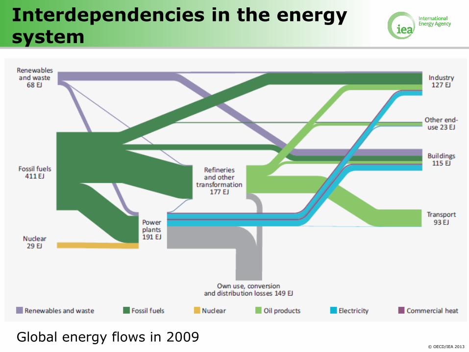
Interdependencies in the energy system
Global energy flows in 2009
© OECD/IEA 2013
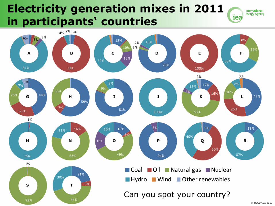
Electricity generation mixes in 2011 in participants‘ countries
44%
1%14%
23%
3%6%
9%
Coal Oil Natural gas Nuclear Hydro Wind Other renewables
5%3%
81%
6%
3%
90%
4% 2%
12%
10%
15%59%
79%
2%2% 15%
100%
8%
24%
68%
44%
23%
20%
7%5%
59%
7%
33%
81%
9%
9%
100%
12%
16%
53%
3%
12%
3%
47%
26%
16%
8%
3%
1%
98%
16%
63%
21% 16%
3%
49%
16%
16%
94%
5% 9%
50%
40%
13%
87%
99%
1%
44%
1%14%
23%
3%6%
9%
Coal Oil Natural gas Nuclear Hydro Wind Other renewables21%
5%
44%
30%
Can you spot your country?
A B C D E F
G H I J K L
M N O P Q R
S T
© OECD/IEA 2013
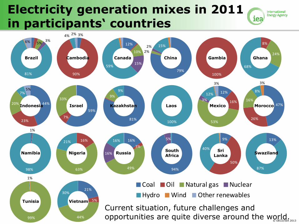
Electricity generation mixes in 2011 in participants‘ countries
44%
1%14%
23%
3%6%
9%
Coal Oil Natural gas Nuclear Hydro Wind Other renewables
5%3%
81%
6%
3%
90%
4% 2%
12%
10%
15%59%
79%
2%2% 15%
100%
8%
24%
68%
44%
23%
20%
7%5%
59%
7%
33%
81%
9%
9%
100%
12%
16%
53%
3%
12%
3%
47%
26%
16%
8%
3%
1%
98%
16%
63%
21% 16%
3%
49%
16%
16%
94%
5% 9%
50%
40%
13%
87%
99%
1%
Current situation, future challenges and opportunities are quite diverse around the world.
Brazil Cambodia Canada China Gambia Ghana
Indonesia Israel Kazakhstan Laos Mexico Morocco
Namibia Nigeria Russia South Africa
Sri Lanka
Swaziland
Tunisia
44%
1%14%
23%
3%6%
9%
Coal Oil Natural gas Nuclear Hydro Wind Other renewables21%
5%
44%
30%
Vietnam
© OECD/IEA 2013
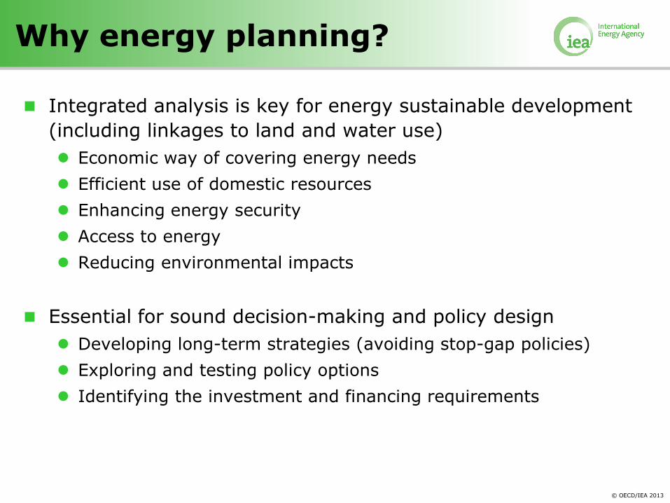
Why energy planning?
Integrated analysis is key for energy sustainable development
(including linkages to land and water use)
Economic way of covering energy needs
Efficient use of domestic resources
Enhancing energy security
Access to energy
Reducing environmental impacts
Essential for sound decision-making and policy design
Developing long-term strategies (avoiding stop-gap policies)
Exploring and testing policy options
Identifying the investment and financing requirements
© OECD/IEA 2013
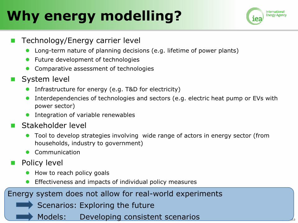
Why energy modelling?
Technology/Energy carrier level
Long-term nature of planning decisions (e.g. lifetime of power plants)
Future development of technologies
Comparative assessment of technologies
System level
Infrastructure for energy (e.g. T&D for electricity)
Interdependencies of technologies and sectors (e.g. electric heat pump or EVs with
power sector)
Integration of variable renewables
Stakeholder level
Tool to develop strategies involving wide range of actors in energy sector (from
households, industry to government)
Communication
Policy level
How to reach policy goals
Effectiveness and impacts of individual policy measures
Energy system does not allow for real-world experiments
Scenarios: Exploring the future
Models: Developing consistent scenarios
© OECD/IEA 2013
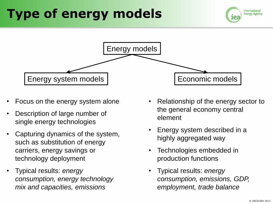
Type of energy models
Energy system models
Energy models
Economic models
• Focus on the energy system alone
• Description of large number of
single energy technologies
• Capturing dynamics of the system,
such as substitution of energy
carriers, energy savings or
technology deployment
• Typical results: energy
consumption, energy technology
mix and capacities, emissions
• Relationship of the energy sector to
the general economy central
element
• Energy system described in a
highly aggregated way
• Technologies embedded in
production functions
• Typical results: energy
consumption, emissions, GDP,
employment, trade balance
© OECD/IEA 2013
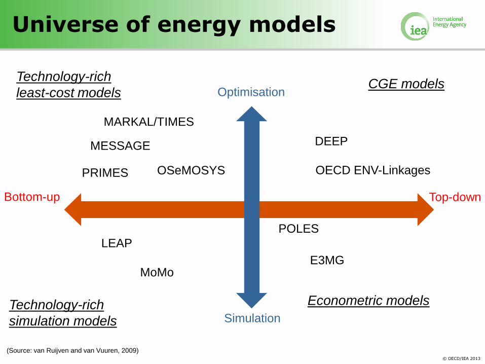
Optimisation
Simulation
Top-down Bottom-up
E3MG
Econometric models
POLES
MARKAL/TIMES
MESSAGE
PRIMES
Technology-rich
least-cost models
OSeMOSYS
DEEP
CGE models
OECD ENV-Linkages
LEAP
Technology-rich
simulation models
MoMo
(Source: van Ruijven and van Vuuren, 2009)
Universe of energy models
© OECD/IEA 2013
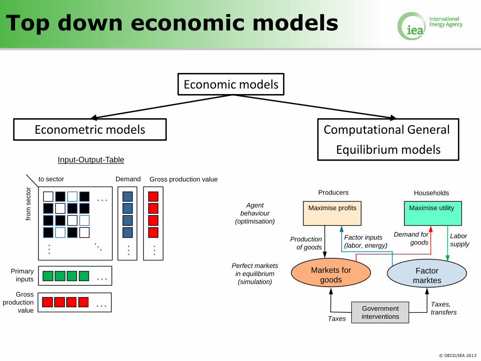
Top down economic models
Economic models
Econometric models
…
…
…
…
…
…
from
secto
r
to sector Demand Gross production value
Primary
inputs
Gross
production
value
Input-Output-Table
Computational General
Equilibrium models
Producers Households
Maximise profits Maximise utility
Perfect markets
in equilibrium
(simulation)
Government
interventions
Demand for
goods Production
of goods
Factor inputs
(labor, energy)
Labor
supply
Markets for
goods Factor
marktes
Taxes
Taxes,
transfers
Agent
behaviour
(optimisation)
© OECD/IEA 2013
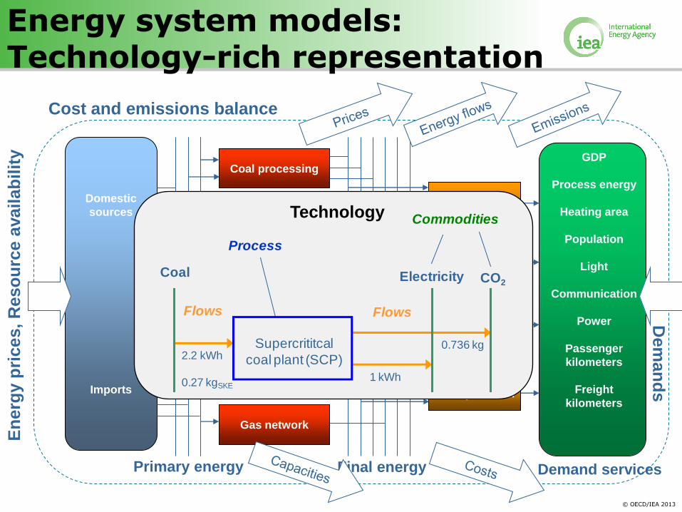
Energy system models: Technology-rich representation
Cost and emissions balance
GDP
Process energy
Heating area
Population
Light
Communication
Power
Passenger
kilometers
Freight
kilometers
Demand services
Coal processing
Refineries
Power plants
and
Transportation
CHP plants
and district
heat networks
Gas network
Industry
Commercial and
tertiary sector
Households
Transportation
Final energy Primary energy
Domestic
sources
Imports
En
erg
y p
rices,
Reso
urc
e a
vailab
ilit
y
Dem
an
ds
ElectricityCoal
Supercrititcal
coal plant (SCP)
CO2
Process
Commodities
FlowsFlows
2.2 kWh
1 kWh0.27 kgSKE
0.736 kg
Technology
© OECD/IEA 2013
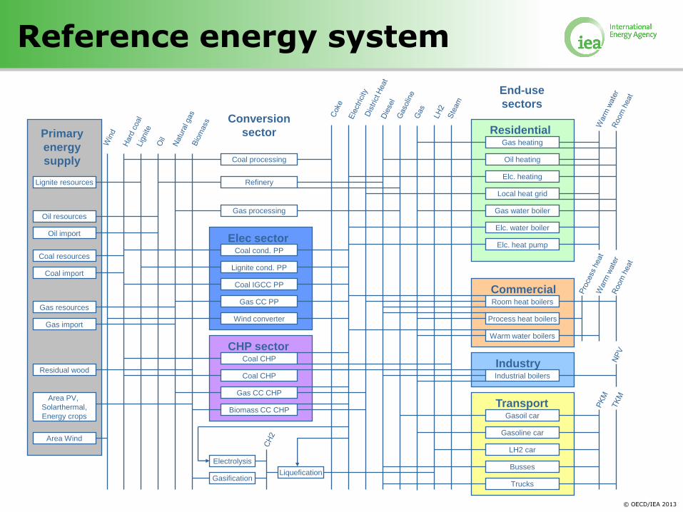
Reference energy system
Gas heating
Oil heating
Elc. heating
Local heat grid
Gas water boiler
Elc. water boiler
Room heat boilers
Process heat boilers
Industrial boilers
LH2 car
Busses
Gasoline car
Gasoil car
Elc. heat pump
Warm water boilers
Trucks
Coal processing
Refinery
Gas processing
Coal cond. PP
Lignite cond. PP
Coal IGCC PP
Gas CC PP
Wind converter
Coal CHP
Coal CHP
Gas CC CHP
Biomass CC CHP
Electrolysis
Gasification Liquefication
Area PV,
Solarthermal,
Energy crops
Area Wind
Residual wood
Gas import
Gas resources
Coal import
Coal resources
Oil resources
Oil import
Lignite resources
Industry
Transport
Commercial
Residential
Elec sector
CHP sector
Primary
energy
supply
Conversion
sector
End-use
sectors
© OECD/IEA 2013
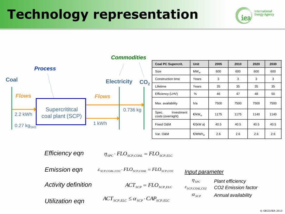
Technology representation
Electricity Coal
Supercrititcal
coal plant (SCP)
CO2
Process
Commodities
Flows Flows
Coal PC Supercrit. Unit 2005 2010 2020 2030
Size MWel 600 600 600 600
Construction time Years 3 3 3 3
Lifetime Years 35 35 35 35
Efficiency (LHV) % 46 47 48 50
Max. availability h/a 7500 7500 7500 7500
Spec. Investment
costs (overnight) €/kWel 1175 1175 1140 1140
Fixed O&M €/(kW a) 40.5 40.5 40.5 40.5
Var. O&M €/MWhel 2.6 2.6 2.6 2.6
2.2 kWh
1 kWh 0.27 kgSKE
0.736 kg
ELCSCPCOALSCPSPC FLOFLO ,,
2,,2,, COSCPCOALSCPCOCOALSCP FLOFLO
ELCSCPSCPELCSCP CAPACT ,,
ELCSCPSCP FLOACT ,
Efficiency eqn
Emission eqn
Activity definition
Utilization eqn
SPC Plant efficiency
O2SCP,COAL,Cε CO2 Emission factor
SCP Annual availability
Input parameter
© OECD/IEA 2013
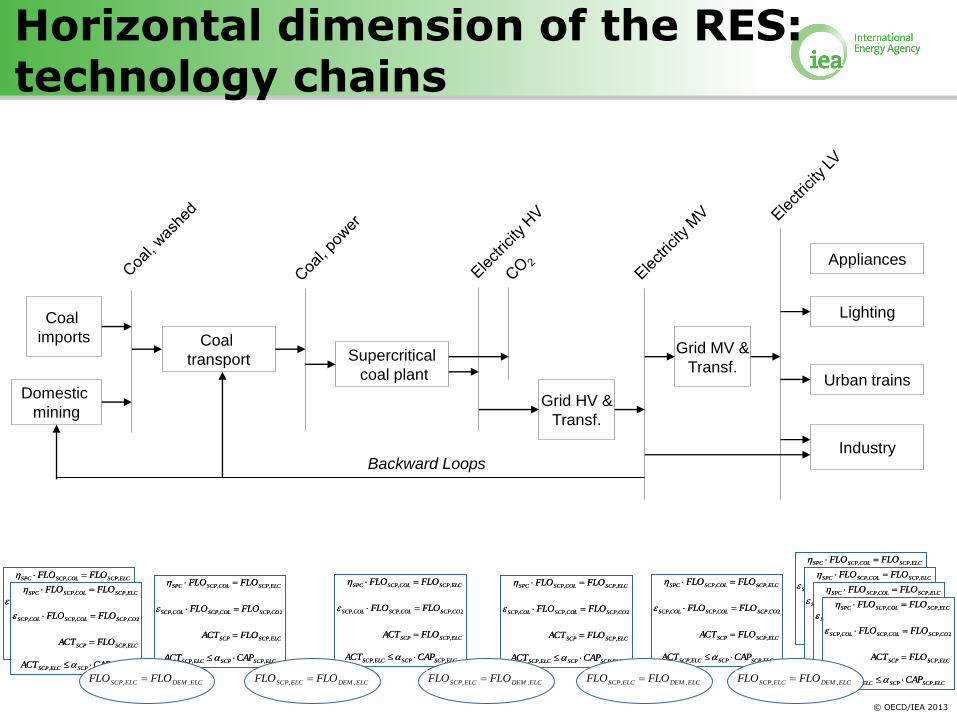
Horizontal dimension of the RES: technology chains
Supercritical
coal plant
Coal
transport
Grid HV &
Transf.
Lighting
Urban trains
Industry
Domestic
mining
Coal
imports Grid MV &
Transf.
ELCSCPCOLSCPSPC FLOFLO ,,
2,,, COSCPCOLSCPCOLSCP FLOFLO
ELCSCPSCPELCSCP CAPACT ,,
ELCSCPSCP FLOACT ,
ELCSCPCOLSCPSPC FLOFLO ,,
2,,, COSCPCOLSCPCOLSCP FLOFLO
ELCSCPSCPELCSCP CAPACT ,,
ELCSCPSCP FLOACT ,
ELCSCPCOLSCPSPC FLOFLO ,,
2,,, COSCPCOLSCPCOLSCP FLOFLO
ELCSCPSCPELCSCP CAPACT ,,
ELCSCPSCP FLOACT ,
ELCSCPCOLSCPSPC FLOFLO ,,
2,,, COSCPCOLSCPCOLSCP FLOFLO
ELCSCPSCPELCSCP CAPACT ,,
ELCSCPSCP FLOACT ,
ELCSCPCOLSCPSPC FLOFLO ,,
2,,, COSCPCOLSCPCOLSCP FLOFLO
ELCSCPSCPELCSCP CAPACT ,,
ELCSCPSCP FLOACT ,
ELCSCPCOLSCPSPC FLOFLO ,,
2,,, COSCPCOLSCPCOLSCP FLOFLO
ELCSCPSCPELCSCP CAPACT ,,
ELCSCPSCP FLOACT ,
ELCSCPCOLSCPSPC FLOFLO ,,
2,,, COSCPCOLSCPCOLSCP FLOFLO
ELCSCPSCPELCSCP CAPACT ,,
ELCSCPSCP FLOACT ,
ELCSCPCOLSCPSPC FLOFLO ,,
2,,, COSCPCOLSCPCOLSCP FLOFLO
ELCSCPSCPELCSCP CAPACT ,,
ELCSCPSCP FLOACT ,
ELCSCPCOLSCPSPC FLOFLO ,,
2,,, COSCPCOLSCPCOLSCP FLOFLO
ELCSCPSCPELCSCP CAPACT ,,
ELCSCPSCP FLOACT ,
ELCSCPCOLSCPSPC FLOFLO ,,
2,,, COSCPCOLSCPCOLSCP FLOFLO
ELCSCPSCPELCSCP CAPACT ,,
ELCSCPSCP FLOACT ,
ELCSCPCOLSCPSPC FLOFLO ,,
2,,, COSCPCOLSCPCOLSCP FLOFLO
ELCSCPSCPELCSCP CAPACT ,,
ELCSCPSCP FLOACT ,
ELCSCPCOLSCPSPC FLOFLO ,,
2,,, COSCPCOLSCPCOLSCP FLOFLO
ELCSCPSCPELCSCP CAPACT ,,
ELCSCPSCP FLOACT ,
ELCSCPCOLSCPSPC FLOFLO ,,
2,,, COSCPCOLSCPCOLSCP FLOFLO
ELCSCPSCPELCSCP CAPACT ,,
ELCSCPSCP FLOACT ,
ELCSCPCOLSCPSPC FLOFLO ,,
2,,, COSCPCOLSCPCOLSCP FLOFLO
ELCSCPSCPELCSCP CAPACT ,,
ELCSCPSCP FLOACT ,
ELCSCPCOLSCPSPC FLOFLO ,,
2,,, COSCPCOLSCPCOLSCP FLOFLO
ELCSCPSCPELCSCP CAPACT ,,
ELCSCPSCP FLOACT ,
ELCSCPCOLSCPSPC FLOFLO ,,
2,,, COSCPCOLSCPCOLSCP FLOFLO
ELCSCPSCPELCSCP CAPACT ,,
ELCSCPSCP FLOACT ,
ELCSCPCOLSCPSPC FLOFLO ,,
2,,, COSCPCOLSCPCOLSCP FLOFLO
ELCSCPSCPELCSCP CAPACT ,,
ELCSCPSCP FLOACT ,
ELCSCPCOLSCPSPC FLOFLO ,,
2,,, COSCPCOLSCPCOLSCP FLOFLO
ELCSCPSCPELCSCP CAPACT ,,
ELCSCPSCP FLOACT ,
ELCSCPCOLSCPSPC FLOFLO ,,
2,,, COSCPCOLSCPCOLSCP FLOFLO
ELCSCPSCPELCSCP CAPACT ,,
ELCSCPSCP FLOACT ,
ELCSCPCOLSCPSPC FLOFLO ,,
2,,, COSCPCOLSCPCOLSCP FLOFLO
ELCSCPSCPELCSCP CAPACT ,,
ELCSCPSCP FLOACT ,
Appliances
ELCDEMELCSCP FLOFLO ,, ELCDEMELCSCP FLOFLO ,, ELCDEMELCSCP FLOFLO ,, ELCDEMELCSCP FLOFLO ,, ELCDEMELCSCP FLOFLO ,,
Backward Loops
© OECD/IEA 2013
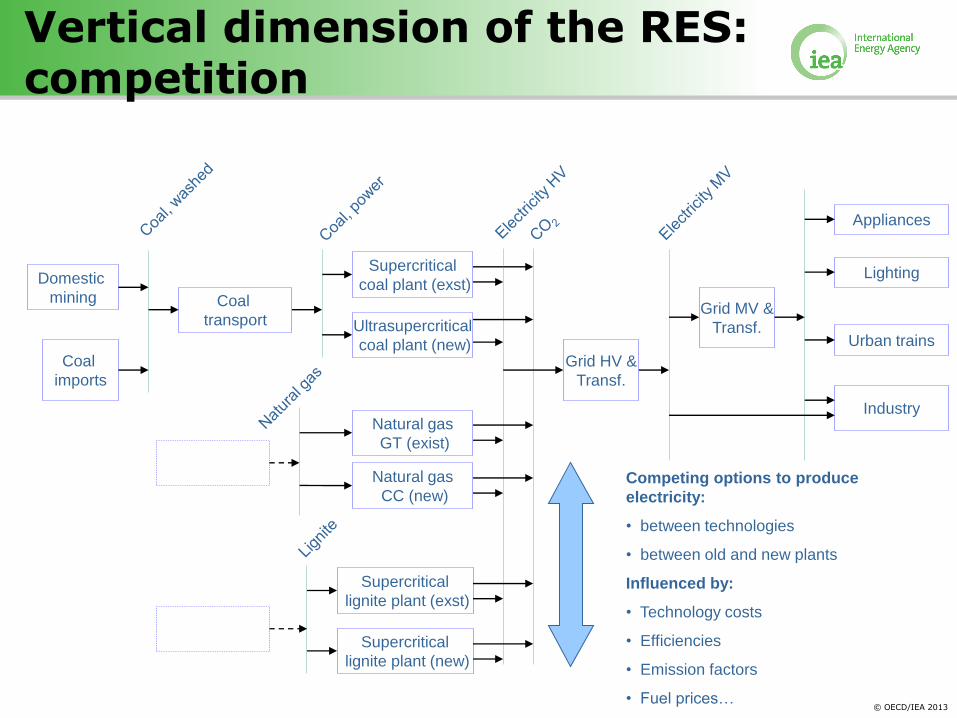
Vertical dimension of the RES: competition
Supercritical
coal plant (exst) Coal
transport
Grid HV &
Transf.
Lighting
Urban trains
Industry
Domestic
mining
Coal
imports
Grid MV &
Transf.
Appliances
Ultrasupercritical
coal plant (new)
Natural gas
GT (exist)
Natural gas
CC (new)
Supercritical
lignite plant (exst)
Supercritical
lignite plant (new)
Competing options to produce
electricity:
• between technologies
• between old and new plants
Influenced by:
• Technology costs
• Efficiencies
• Emission factors
• Fuel prices…
© OECD/IEA 2013
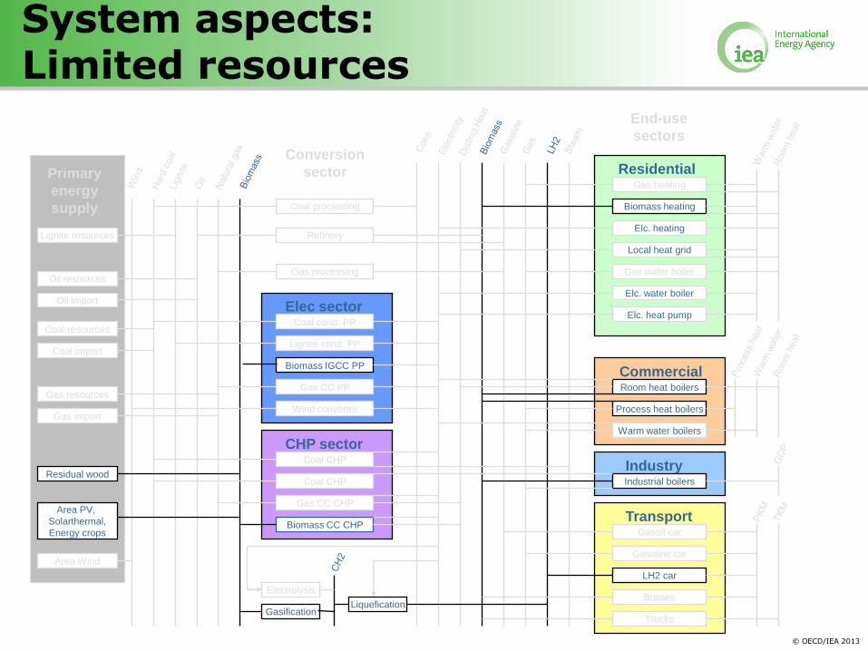
System aspects: Limited resources
Gas heating
Biomass heating
Elc. heating
Local heat grid
Gas water boiler
Elc. water boiler
Room heat boilers
Process heat boilers
Industrial boilers
LH2 car
Busses
Gasoline car
Gasoil car
Elc. heat pump
Warm water boilers
Trucks
Coal processing
Refinery
Gas processing
Coal cond. PP
Lignite cond. PP
Biomass IGCC PP
Gas CC PP
Wind converter
Coal CHP
Coal CHP
Gas CC CHP
Biomass CC CHP
Electrolysis
Gasification Liquefication
Area PV,
Solarthermal,
Energy crops
Area Wind
Residual wood
Gas import
Gas resources
Coal import
Coal resources
Oil resources
Oil import
Lignite resources
Industry
Transport
Commercial
Residential
Elec sector
CHP sector
Primary
energy
supply
Conversion
sector
End-use
sectors
© OECD/IEA 2013
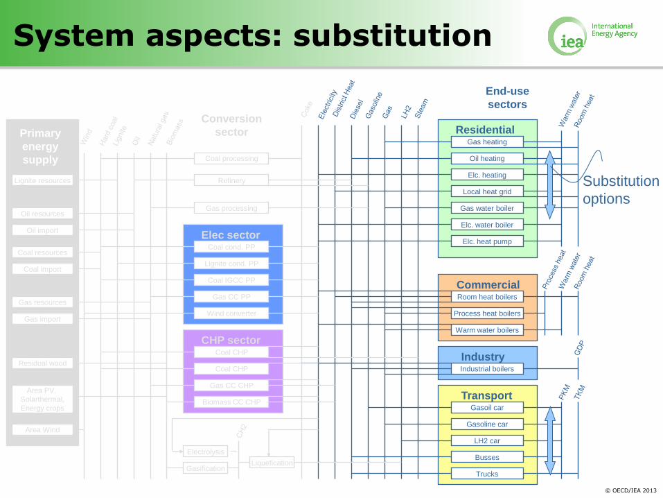
System aspects: substitution
Gas heating
Oil heating
Elc. heating
Local heat grid
Gas water boiler
Elc. water boiler
Room heat boilers
Process heat boilers
Industrial boilers
LH2 car
Busses
Gasoline car
Gasoil car
Elc. heat pump
Warm water boilers
Trucks
Coal processing
Refinery
Gas processing
Coal cond. PP
Lignite cond. PP
Coal IGCC PP
Gas CC PP
Wind converter
Coal CHP
Coal CHP
Gas CC CHP
Biomass CC CHP
Electrolysis
Gasification Liquefication
Area PV,
Solarthermal,
Energy crops
Area Wind
Residual wood
Gas import
Gas resources
Coal import
Coal resources
Oil resources
Oil import
Lignite resources
Industry
Transport
Commercial
Residential
Elec sector
CHP sector
Primary
energy
supply
Conversion
sector
End-use
sectors
Substitution
options
© OECD/IEA 2013
Gas heating
Oil heating
Elc. heating
Local heat grid
Gas water boiler
Elc. water boiler
Room heat boilers
Process heat boilers
Industrial boilers
LH2 car
Busses
Gasoline car
Gasoil car
Elc. heat pump
Warm water boilers
Trucks
Coal processing
Refinery
Gas processing
Coal cond. PP
Lignite cond. PP
Coal IGCC PP
Gas CC PP
Wind converter
Coal CHP
Coal CHP
Gas CC CHP
Biomass CC CHP
Electrolysis
Gasification Liquefication
Area PV,
Solarthermal,
Energy crops
Area Wind
Residual wood
Gas import
Gas resources
Coal import
Coal resources
Oil resources
Oil import
Lignite resources
Industry
Transport
Commercial
Residential
Elec sector
CHP sector
Primary
energy
supply
Conversion
sector
End-use
sectors
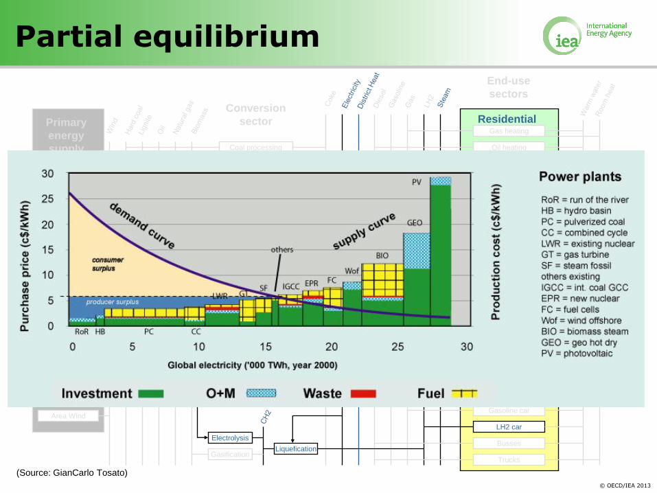
Partial equilibrium
(Source: GianCarlo Tosato)
© OECD/IEA 2013
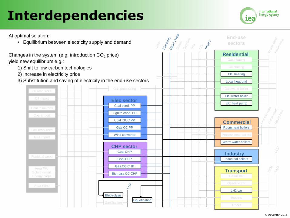
Interdependencies
Gas heating
Oil heating
Elc. heating
Local heat grid
Gas water boiler
Elc. water boiler
Room heat boilers
Process heat boilers
Industrial boilers
LH2 car
Busses
Gasoline car
Gasoil car
Elc. heat pump
Warm water boilers
Trucks
Coal processing
Refinery
Gas processing
Coal cond. PP
Lignite cond. PP
Coal IGCC PP
Gas CC PP
Wind converter
Coal CHP
Coal CHP
Gas CC CHP
Biomass CC CHP
Electrolysis
Gasification Liquefication
Area PV,
Solarthermal,
Energy crops
Area Wind
Residual wood
Gas import
Gas resources
Coal import
Coal resources
Oil resources
Oil import
Lignite resources
Industry
Transport
Commercial
Residential
Elec sector
CHP sector
Primary
energy
supply
Conversion
sector
End-use
sectors
At optimal solution:
• Equilibrium between electricity supply and demand
Changes in the system (e.g. introduction CO2 price)
yield new equilibrium e.g.:
1) Shift to low-carbon technologies
2) Increase in electricity price
3) Substitution and saving of electricity in the end-use sectors
© OECD/IEA 2013
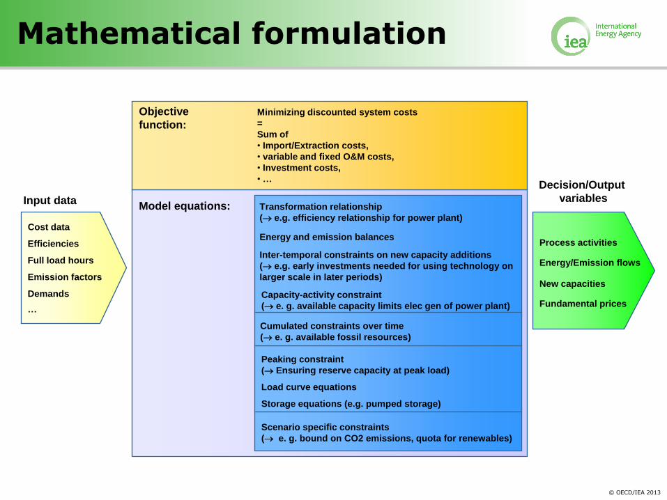
Mathematical formulation
Minimizing discounted system costs
=
Sum of
• Import/Extraction costs,
• variable and fixed O&M costs,
• Investment costs,
• …
Transformation relationship
( e.g. efficiency relationship for power plant)
Energy and emission balances
Capacity-activity constraint
( e. g. available capacity limits elec gen of power plant)
Peaking constraint
( Ensuring reserve capacity at peak load)
Scenario specific constraints
( e. g. bound on CO2 emissions, quota for renewables)
Inter-temporal constraints on new capacity additions
( e.g. early investments needed for using technology on
larger scale in later periods)
Storage equations (e.g. pumped storage)
Cumulated constraints over time
( e. g. available fossil resources)
Objective
function:
Model equations:
Cost data
Efficiencies
Full load hours
Emission factors
Demands
…
Input data
Energy/Emission flows
Process activities
New capacities
Fundamental prices
Decision/Output
variables
Load curve equations
© OECD/IEA 2013
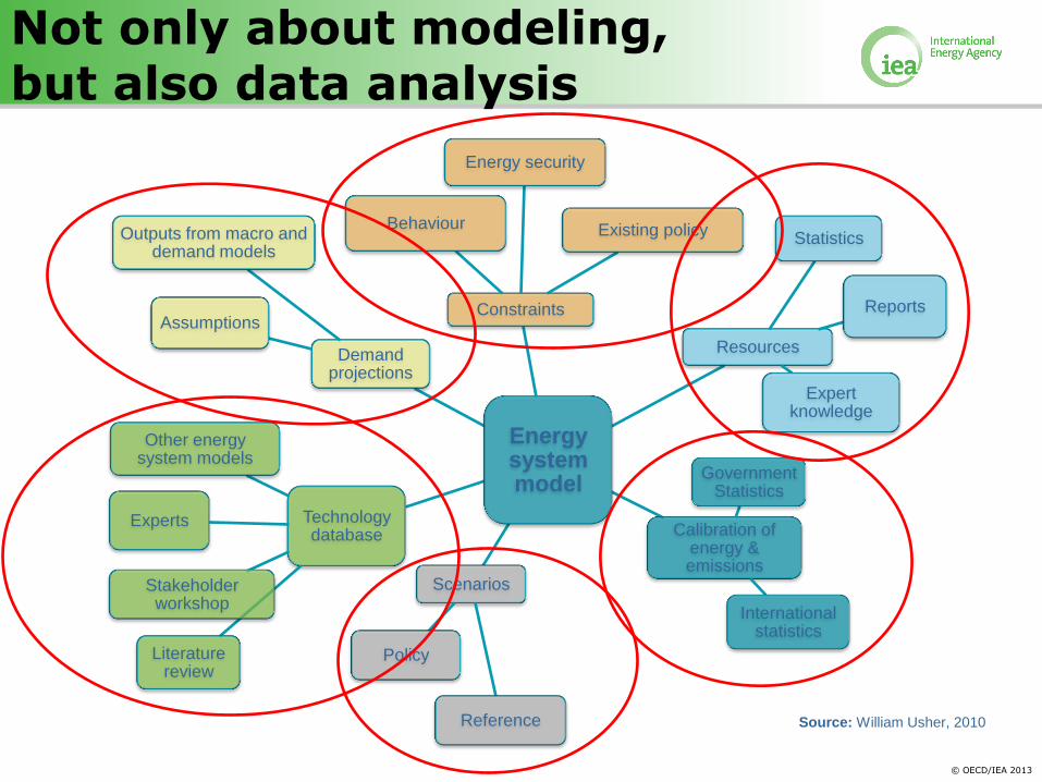
Energy system model
Constraints
Energy security
Existing policy Behaviour
Resources
Statistics
Expert knowledge
Reports
Calibration of energy & emissions
Government Statistics
International statistics
Scenarios
Reference
Policy
Technology database
Experts
Literature review
Stakeholder workshop
Other energy system models
Demand projections
Outputs from macro and demand models
Assumptions
Source: William Usher, 2010
Not only about modeling, but also data analysis
© OECD/IEA 2013
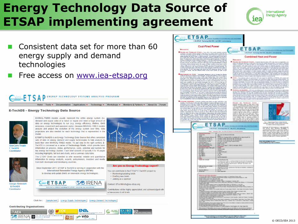
Energy Technology Data Source of ETSAP implementing agreement
Consistent data set for more than 60 energy supply and demand technologies
Free access on www.iea-etsap.org

© OECD/IEA 2013
Getting a free evaluation license for ETSAP tools
To test ETSAP’s modelling tools,
visit http://iea-etsap.org/web/AcquiringETSAP_Tools.asp
and get a free 60-day evaluation license.
© OECD/IEA 2013
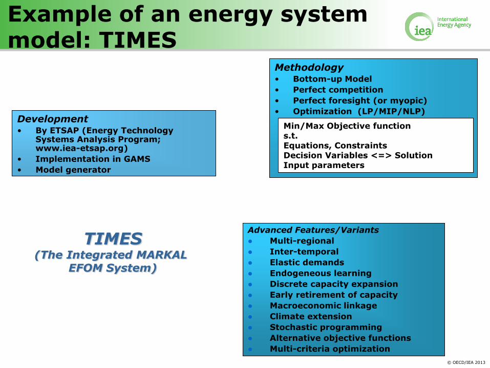
Advanced Features/Variants
● Multi-regional
● Inter-temporal
● Elastic demands
● Endogeneous learning
● Discrete capacity expansion
● Early retirement of capacity
● Macroeconomic linkage
● Climate extension
● Stochastic programming
● Alternative objective functions
● Multi-criteria optimization
Methodology • Bottom-up Model
• Perfect competition
• Perfect foresight (or myopic)
• Optimization (LP/MIP/NLP)
Min/Max Objective function s.t. Equations, Constraints Decision Variables <=> Solution Input parameters
Development • By ETSAP (Energy Technology
Systems Analysis Program; www.iea-etsap.org)
• Implementation in GAMS
• Model generator
TIMES (The Integrated MARKAL
EFOM System)
Example of an energy system model: TIMES
© OECD/IEA 2013
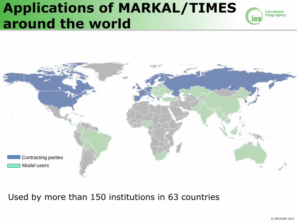
Applications of MARKAL/TIMES around the world
Used by more than 150 institutions in 63 countries
Contracting parties
Model users
© OECD/IEA 2013
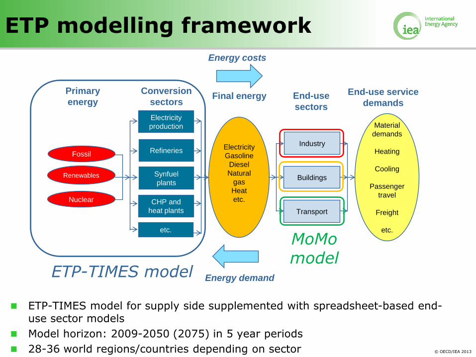
ETP-TIMES model for supply side supplemented with spreadsheet-based end-use sector models
Model horizon: 2009-2050 (2075) in 5 year periods
28-36 world regions/countries depending on sector
Primary
energy
Conversion
sectors Final energy End-use
sectors
End-use service
demands
Electricity
production
Fossil
Renewables
Nuclear
Refineries
Synfuel
plants
CHP and
heat plants
etc.
Electricity
Gasoline
Diesel
Natural
gas
Heat
etc.
Industry
Buildings
Transport
Material
demands
Heating
Cooling
Passenger
travel
Freight
etc.
ETP-TIMES model
MoMo model
Energy costs
Energy demand
ETP modelling framework
© OECD/IEA 2013
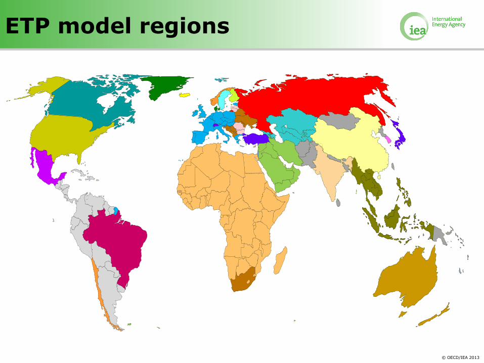
ETP model regions
© OECD/IEA 2013
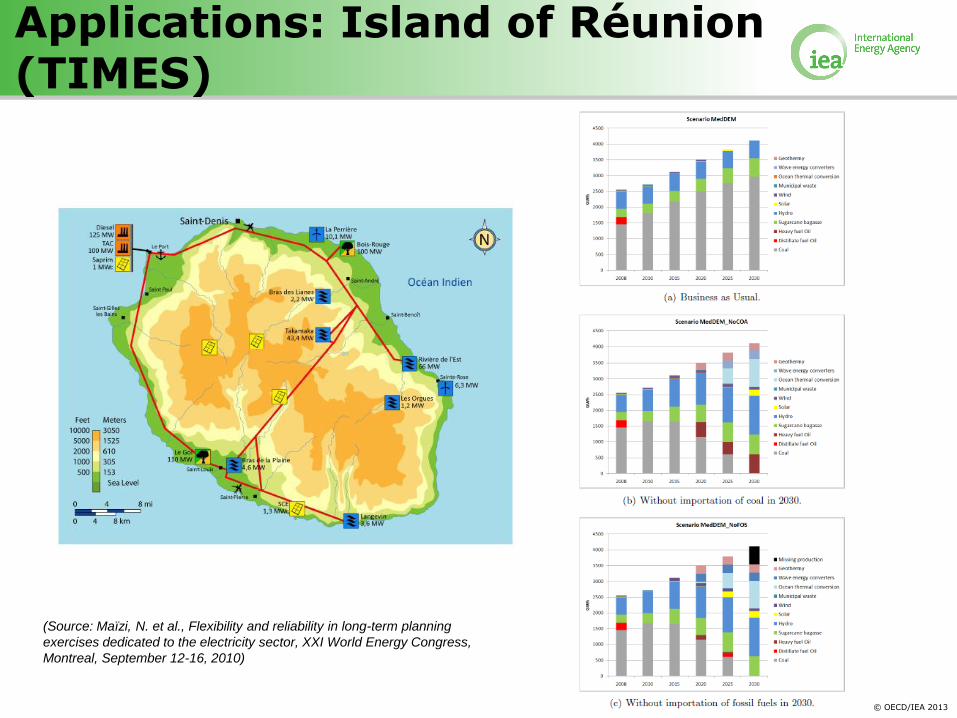
Applications: Island of Réunion (TIMES)
(Source: Maïzi, N. et al., Flexibility and reliability in long-term planning
exercises dedicated to the electricity sector, XXI World Energy Congress,
Montreal, September 12-16, 2010)
© OECD/IEA 2013
Experience with energy models in your organisation?
Which energy models are used in your country or
region?
Discussion
© OECD/IEA 2013
Summary
Energy models provide a consistent analysis framework
Energy models are simplified representation of the real-world
system
Level of detail depends on questions to be addressed and available
data
Choice of model type depending on analysis question
Energy system models: focus on role of technologies and
interactions within the energy sector
Economic models: focus on interdependencies of the energy sector
with the remaining economy
Energy modelling is a long-term and continuous process,
involving experts from different disciplines
Limitations of individual model approaches important when
interpreting model results (no analysis is perfect)
Energy planning not about predicting the future, but supporting
decision making under inherent uncertainties
© OECD/IEA 2013
Getting Started with TIMES:
Running a Power Sector Investment Model
Energy Training Week 2014
8-9 April, 2014
Uwe Remme, Luis Munuera
© OECD/IEA 2013
0
1000
2000
3000
4000
5000
6000
2011 2015 2020 2025 2030 2035 2040 2045 2050
GW
Geothermal
Wind
Solar
Biomass and waste
Nuclear
Oil
Natural gas
Coal
Hydro
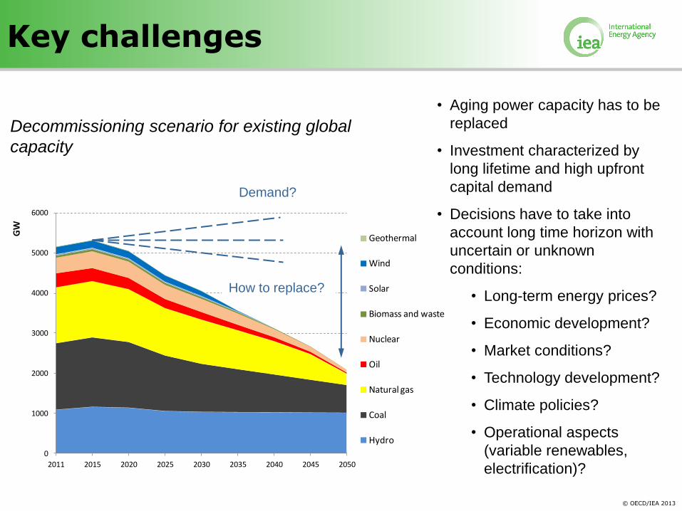
Key challenges
• Aging power capacity has to be
replaced
• Investment characterized by
long lifetime and high upfront
capital demand
• Decisions have to take into
account long time horizon with
uncertain or unknown
conditions:
• Long-term energy prices?
• Economic development?
• Market conditions?
• Technology development?
• Climate policies?
• Operational aspects
(variable renewables,
electrification)?
Demand?
How to replace?
Decommissioning scenario for existing global
capacity
© OECD/IEA 2013
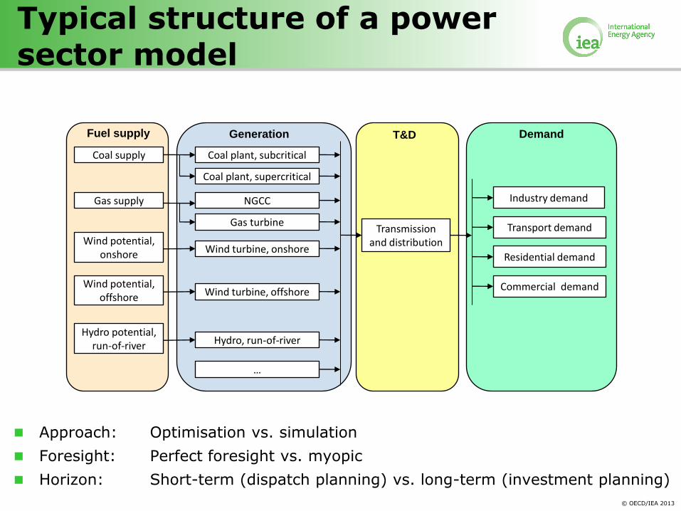
Typical structure of a power sector model
Wind turbine, onshore
Wind turbine, offshore
Hydro, run-of-river
Gas turbine
NGCC
Coal plant, supercritical
Coal plant, subcritical Coal supply
Gas supply
Wind potential, onshore
Wind potential, offshore
Hydro potential, run-of-river
Transmission and distribution
…
Industry demand
Transport demand
Residential demand
Commercial demand
Fuel supply Generation T&D Demand
Approach: Optimisation vs. simulation
Foresight: Perfect foresight vs. myopic
Horizon: Short-term (dispatch planning) vs. long-term (investment planning)
© OECD/IEA 2013
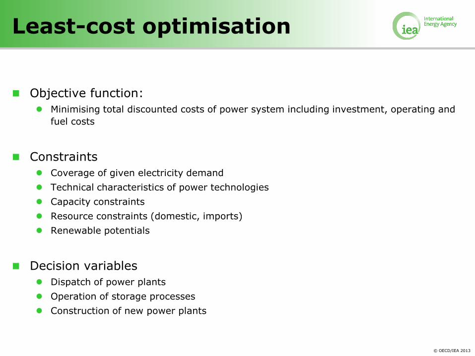
Least-cost optimisation
Objective function:
Minimising total discounted costs of power system including investment, operating and
fuel costs
Constraints
Coverage of given electricity demand
Technical characteristics of power technologies
Capacity constraints
Resource constraints (domestic, imports)
Renewable potentials
Decision variables
Dispatch of power plants
Operation of storage processes
Construction of new power plants
© OECD/IEA 2013
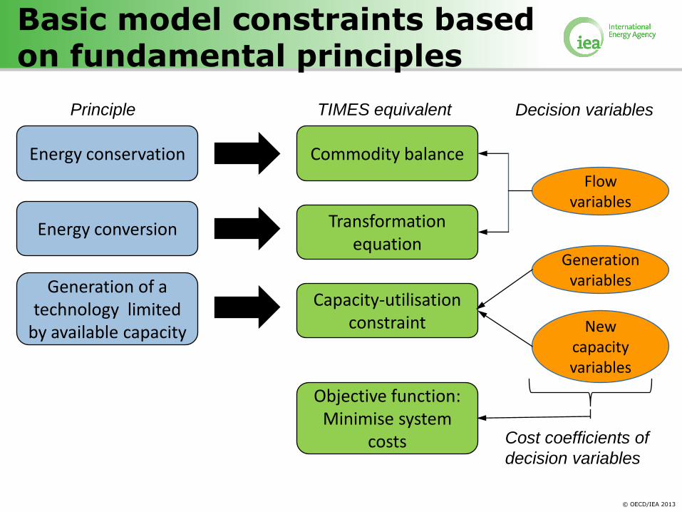
Basic model constraints based on fundamental principles
Energy conversion Transformation equation
Generation of a technology limited
by available capacity
Capacity-utilisation constraint
Energy conservation Commodity balance
TIMES equivalent Principle
Flow variables
Decision variables
New capacity variables
Generation variables
Objective function: Minimise system
costs Cost coefficients of
decision variables
© OECD/IEA 2013
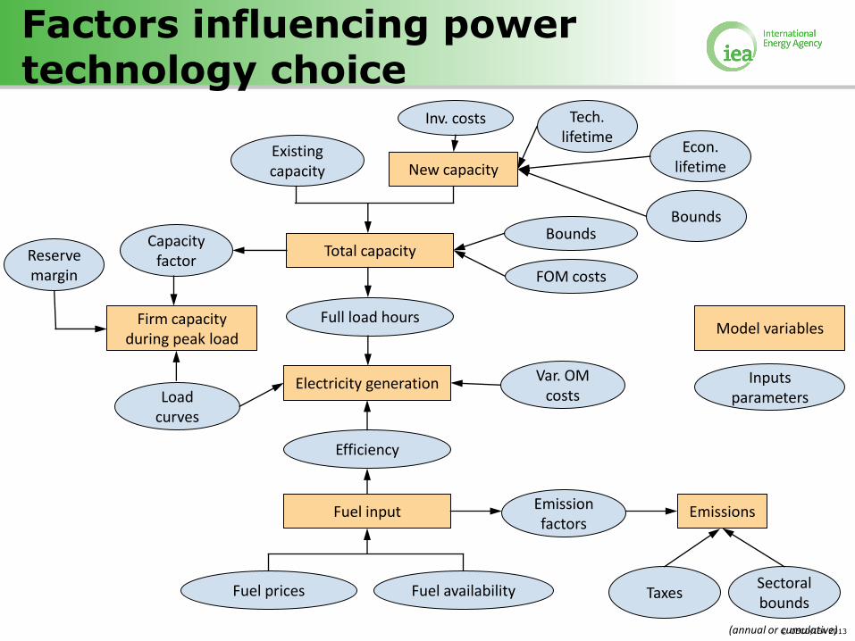
Factors influencing power technology choice
Fuel input
Efficiency
Fuel prices Fuel availability
Emission factors
Emissions
Taxes Sectoral bounds
(annual or cumulative)
Full load hours
Total capacity Bounds
FOM costs
Electricity generation Var. OM costs
Inv. costs Tech. lifetime
Econ. lifetime
Bounds
New capacity Existing capacity
Model variables
Inputs parameters Load
curves
Capacity factor
Firm capacity during peak load
Reserve margin
© OECD/IEA 2013
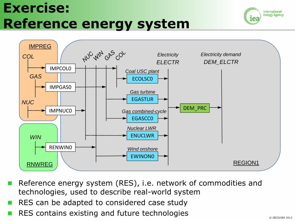
Exercise: Reference energy system
ECOLSC0
EGASTUR
EGASCC0
EWINON0
Electricity
REGION1
DEM_PRC
Electricity demand
DEM_ELCTR IMPCOL0
IMPGAS0
RENWIN0
Coal USC plant
Gas turbine
Gas combined-cycle
Wind onshore
COL
GAS
WIN
ELECTR
IMPREG
RNWREG
Reference energy system (RES), i.e. network of commodities and technologies, used to describe real-world system
RES can be adapted to considered case study
RES contains existing and future technologies
NUC
IMPNUC0
ENUCLWR
Nuclear LWR
© OECD/IEA 2013
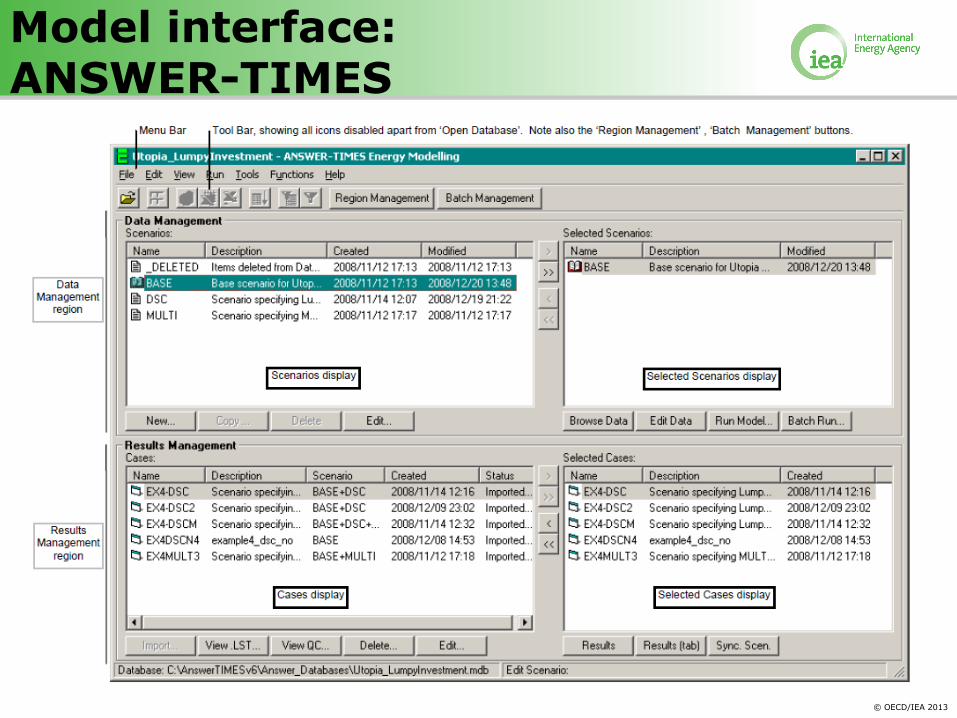
Model interface: ANSWER-TIMES
© OECD/IEA 2013
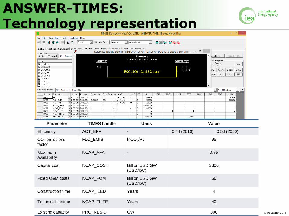
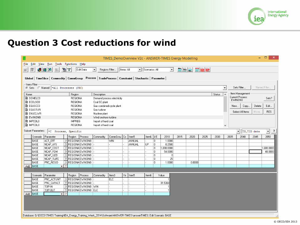
ANSWER-TIMES: Technology representation
Parameter TIMES handle Units Value
Efficiency ACT_EFF - 0.44 (2010) 0.50 (2050)
CO2 emissions factor
FLO_EMIS ktCO2/PJ 95
Maximum availability
NCAP_AFA - 0.85
Capital cost NCAP_COST Billion USD/GW (USD/kW)
2800
Fixed O&M costs NCAP_FOM Billion USD/GW (USD/kW)
56
Construction time NCAP_ILED Years 4
Technical lifetime NCAP_TLIFE Years 40
Existing capacity PRC_RESID GW 300
© OECD/IEA 2013
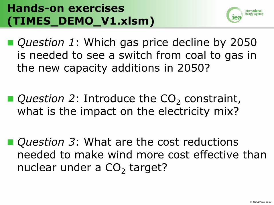
Hands-on exercises (TIMES_DEMO_V1.xlsm)
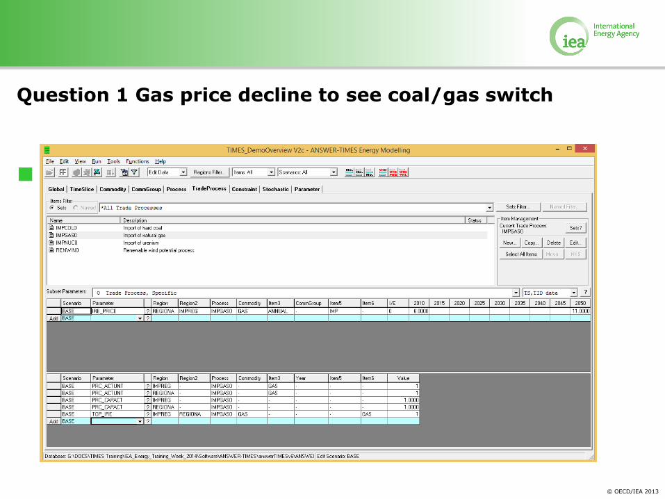
Question 1: Which gas price decline by 2050 is needed to see a switch from coal to gas in the new capacity additions in 2050?
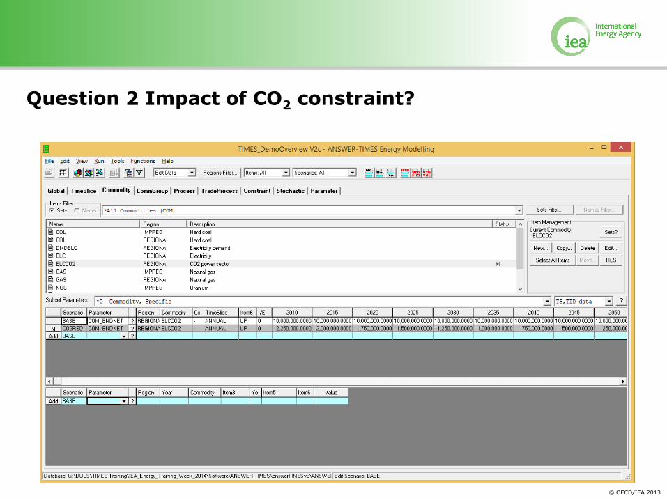
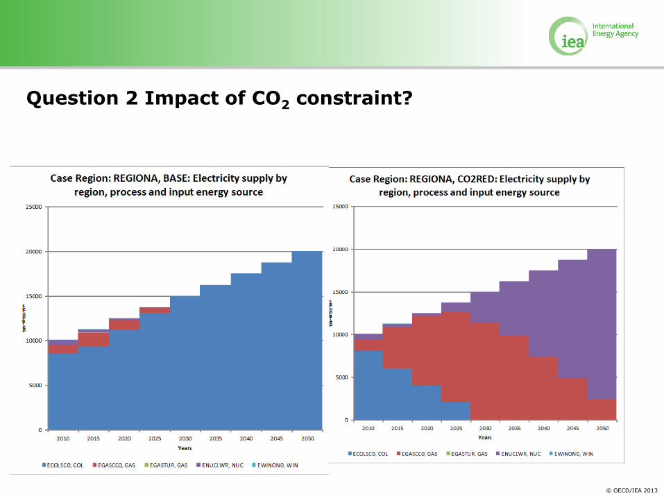
Question 2: Introduce the CO2 constraint, what is the impact on the electricity mix?
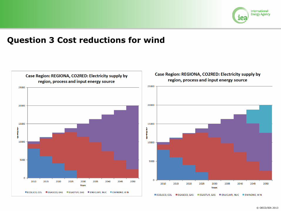
Question 3: What are the cost reductions needed to make wind more cost effective than nuclear under a CO2 target?
© OECD/IEA 2013
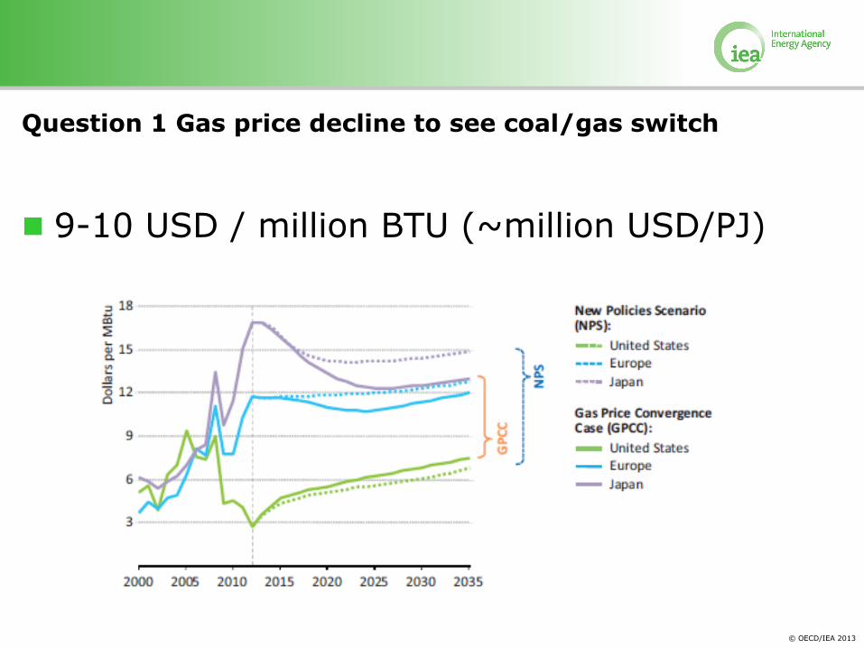
Question 1 Gas price decline to see coal/gas switch
9-10 USD / million BTU (~million USD/PJ)
© OECD/IEA 2013
Question 1 Gas price decline to see coal/gas switch
9-10 USD / million BTU (~million USD/PJ)
© OECD/IEA 2013
Question 2 Impact of CO2 constraint?
© OECD/IEA 2013
Question 2 Impact of CO2 constraint?
© OECD/IEA 2013
Question 3 Cost reductions for wind
© OECD/IEA 2013
Question 3 Cost reductions for wind
© OECD/IEA 2013
Power Sector Modelling with TIMES:
Load curves and storage
Energy Training Week 2014
8-9 April, 2014
Uwe Remme, Luis Munuera
© OECD/IEA 2013
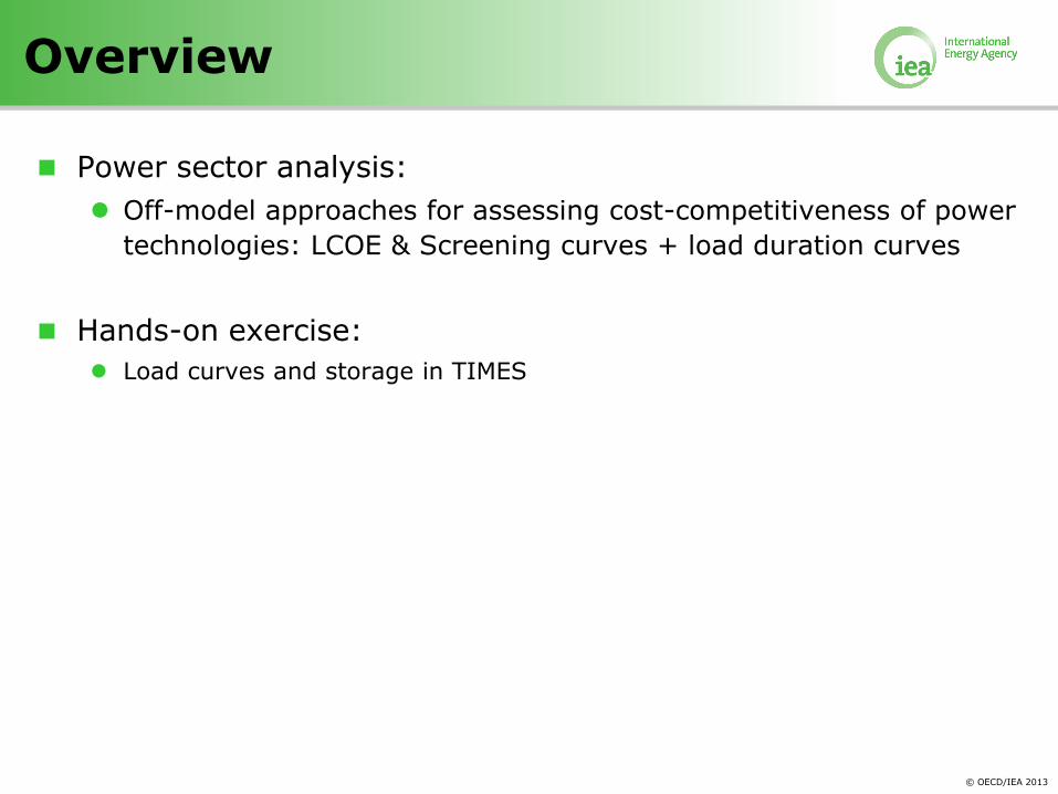
Overview
Power sector analysis:
Off-model approaches for assessing cost-competitiveness of power
technologies: LCOE & Screening curves + load duration curves
Hands-on exercise:
Load curves and storage in TIMES
© OECD/IEA 2013
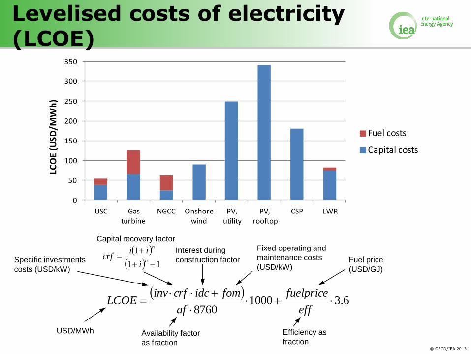
Levelised costs of electricity (LCOE)
0
50
100
150
200
250
300
350
USC Gas turbine
NGCC Onshore wind
PV,utility
PV,rooftop
CSP LWR
LCO
E (U
SD/M
Wh
)
Fuel costs
Capital costs
6.31000
8760
eff
fuelprice
af
fomidccrfinvLCOE
USD/MWh Availability factor
as fraction
Efficiency as
fraction
Fuel price
(USD/GJ)
Fixed operating and
maintenance costs
(USD/kW) Specific investments
costs (USD/kW)
11
1
n
n
i
iicrf
Capital recovery factor
Interest during
construction factor
© OECD/IEA 2013
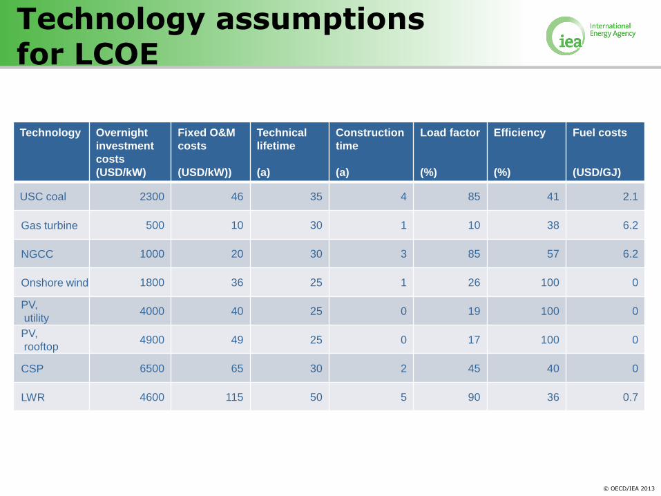
Technology assumptions for LCOE
Technology Overnight
investment
costs
(USD/kW)
Fixed O&M
costs
(USD/kW))
Technical
lifetime
(a)
Construction
time
(a)
Load factor
(%)
Efficiency
(%)
Fuel costs
(USD/GJ)
USC coal 2300 46 35 4 85 41 2.1
Gas turbine 500 10 30 1 10 38 6.2
NGCC 1000 20 30 3 85 57 6.2
Onshore wind 1800 36 25 1 26 100 0
PV,
utility 4000 40 25 0 19 100 0
PV,
rooftop 4900 49 25 0 17 100 0
CSP 6500 65 30 2 45 40 0
LWR 4600 115 50 5 90 36 0.7

© OECD/IEA 2013
Discussion
What are the advantages and disadvantages of the LCOE approach?
© OECD/IEA 2013
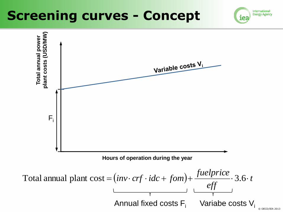
Screening curves - Concept
To
tal a
nn
ua
l p
ow
er
pla
nt
co
sts
(U
SD
/MW
)
Hours of operation during the year
Fi
teff
fuelpricefomidccrfinv 6.3costplant annual Total
Annual fixed costs Fi Variabe costs Vi
© OECD/IEA 2013
0
100
200
300
400
500
600
0% 20% 40% 60% 80% 100%
USD
/(M
Wh
/yr)
Load factor
USC
Gas turbine
NGCC
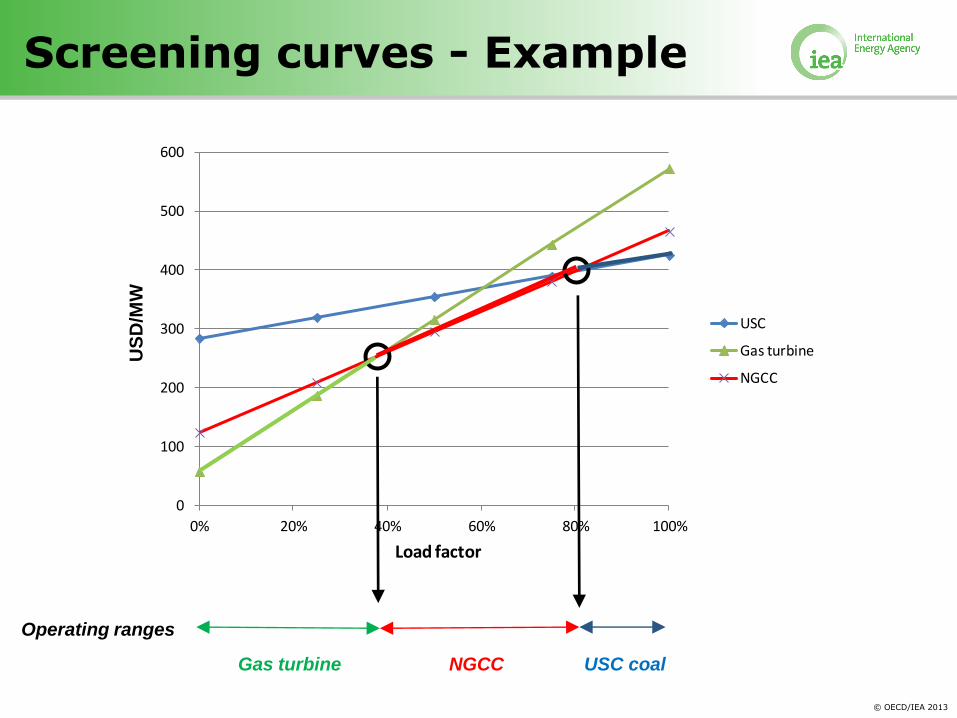
Screening curves - Example
Gas turbine NGCC USC coal
Operating ranges
US
D/M
W
© OECD/IEA 2013
Gas
Oil
Wind
Nuclear
Coal
Hydro
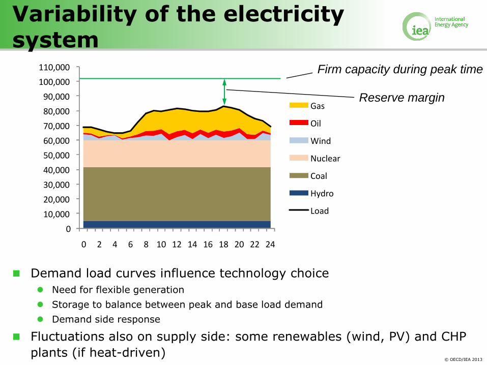
Variability of the electricity system
Demand load curves influence technology choice
Need for flexible generation
Storage to balance between peak and base load demand
Demand side response
Fluctuations also on supply side: some renewables (wind, PV) and CHP
plants (if heat-driven)
Reserve margin
2 4 6 8 10 12 14 16 18 20 22 24
0
10,000
20,000
30,000
40,000
50,000
60,000
70,000
80,000
90,000
100,000
110,000
0
Load
Firm capacity during peak time
© OECD/IEA 2013
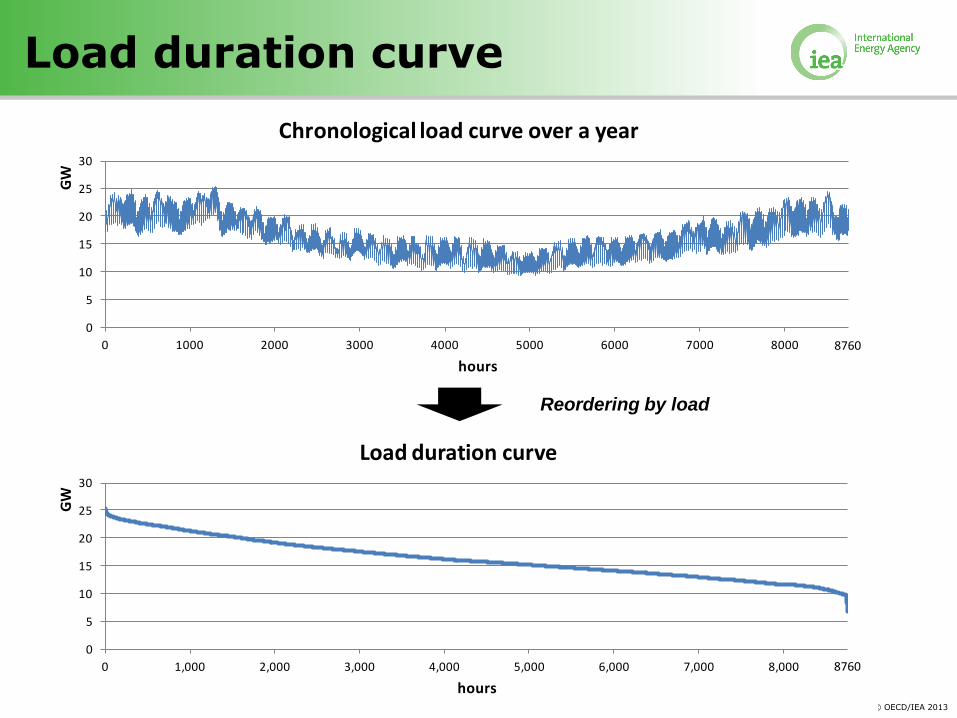
Load duration curve
0
5
10
15
20
25
30
0 1000 2000 3000 4000 5000 6000 7000 8000
GW
hours
Chronological load curve over a year
0
5
10
15
20
25
30
0 1,000 2,000 3,000 4,000 5,000 6,000 7,000 8,000
GW
hours
Load duration curve
Reordering by load
8760
8760
© OECD/IEA 2013
0
5
10
15
20
25
30
0.00
010.
0219
0.04
370.
0655
0.08
730.
1091
0.13
090.
1527
0.17
450.
1963
0.21
820.
2400
0.26
180.
2836
0.30
540.
3272
0.34
900.
3708
0.39
260.
4144
0.43
620.
4580
0.47
980.
5016
0.52
340.
5452
0.56
700.
5888
0.61
060.
6324
0.65
420.
6760
0.69
780.
7196
0.74
140.
7632
0.78
500.
8068
0.82
870.
8505
0.87
230.
8941
0.91
590.
9377
0.95
950.
9813
GW
Load factor
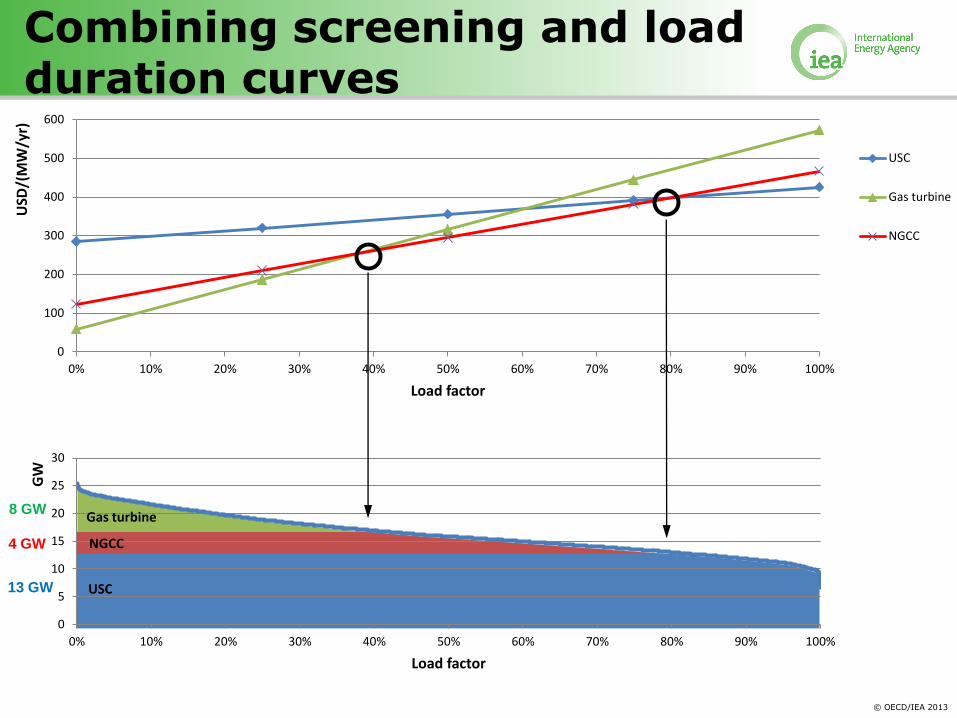
Combining screening and load duration curves
0
100
200
300
400
500
600
0% 10% 20% 30% 40% 50% 60% 70% 80% 90% 100%
USD
/(M
W/y
r)
Load factor
USC
Gas turbine
NGCC
0
5
10
15
20
25
30
0.00
010.
0219
0.04
370.
0655
0.08
730.
1091
0.13
090.
1527
0.17
450.
1963
0.21
820.
2400
0.26
180.
2836
0.30
540.
3272
0.34
900.
3708
0.39
260.
4144
0.43
620.
4580
0.47
980.
5016
0.52
340.
5452
0.56
700.
5888
0.61
060.
6324
0.65
420.
6760
0.69
780.
7196
0.74
140.
7632
0.78
500.
8068
0.82
870.
8505
0.87
230.
8941
0.91
590.
9377
0.95
950.
9813
GW
Load factor
0
5
10
15
20
25
30
0% 10% 20% 30% 40% 50% 60% 70% 80% 90% 100%
GW
Load factor
Load duration curve
13 GW
4 GW
8 GW
USC
NGCC
Gas turbine

© OECD/IEA 2013
Discussion
What are the advantages and disadvantages of the screening curve and load curve approach?
© OECD/IEA 2013
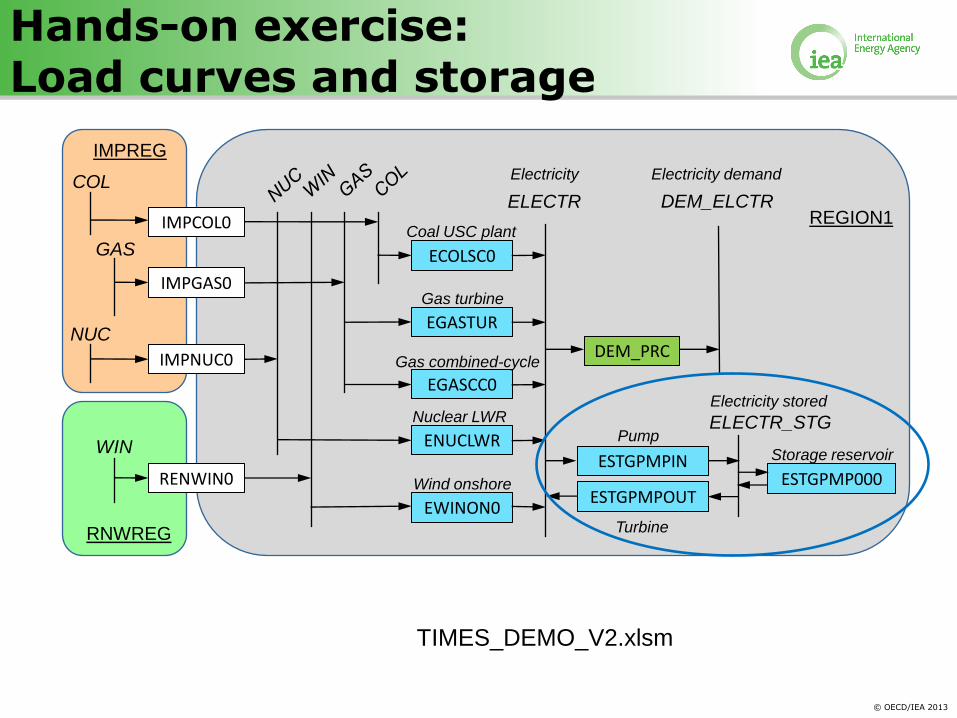
Hands-on exercise: Load curves and storage
ECOLSC0
EGASTUR
EGASCC0
EWINON0
Electricity
REGION1
DEM_PRC
Electricity demand
DEM_ELCTR IMPCOL0
IMPGAS0
RENWIN0
Coal USC plant
Gas turbine
Gas combined-cycle
Wind onshore
COL
GAS
WIN
ELECTR
IMPREG
RNWREG
NUC
IMPNUC0
ENUCLWR
Nuclear LWR
ESTGPMPIN
ESTGPMPOUT
ELECTR_STG
Electricity stored
ESTGPMP000
Turbine
Pump
Storage reservoir
TIMES_DEMO_V2.xlsm
© OECD/IEA 2013
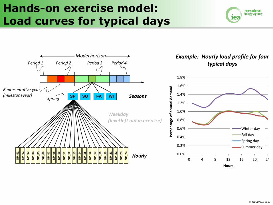
Hands-on exercise model: Load curves for typical days
Example: Hourly load profile for four typical days
0.0%
0.2%
0.4%
0.6%
0.8%
1.0%
1.2%
1.4%
1.6%
1.8%
0 4 8 12 16 20 24
Pe
rce
nta
ge o
f an
nu
al d
em
and
Hours
Winter day
Fall day
Spring day
Summer day
Period 4Period 3Period 2Period 1
Model horizon
Seasons
Weekday (level left out in exercise)
Hourly
WISU FA
Representative year(milestoneyear)
Spring
SP
_01
SP
_02
SP
_03
SP
_04
SP
_05
SP
_06
SP
_07
SP
_08
SP
_10
SP
_11
SP
_12
SP
_13
SP
_14
SP
_15
SP
_16
SP
_17
SP
_19
SP
_20
SP
_21
SP
_22
SP
_23
SP
_24
SP
© OECD/IEA 2013
0.0
0.2
0.4
0.6
0.8
1.0
1.2
0 2 4 6 8 10 12 14 16 18 20 22 24 26 28
Cap
acit
y fa
cto
r (-)
Wind speed (m/s)
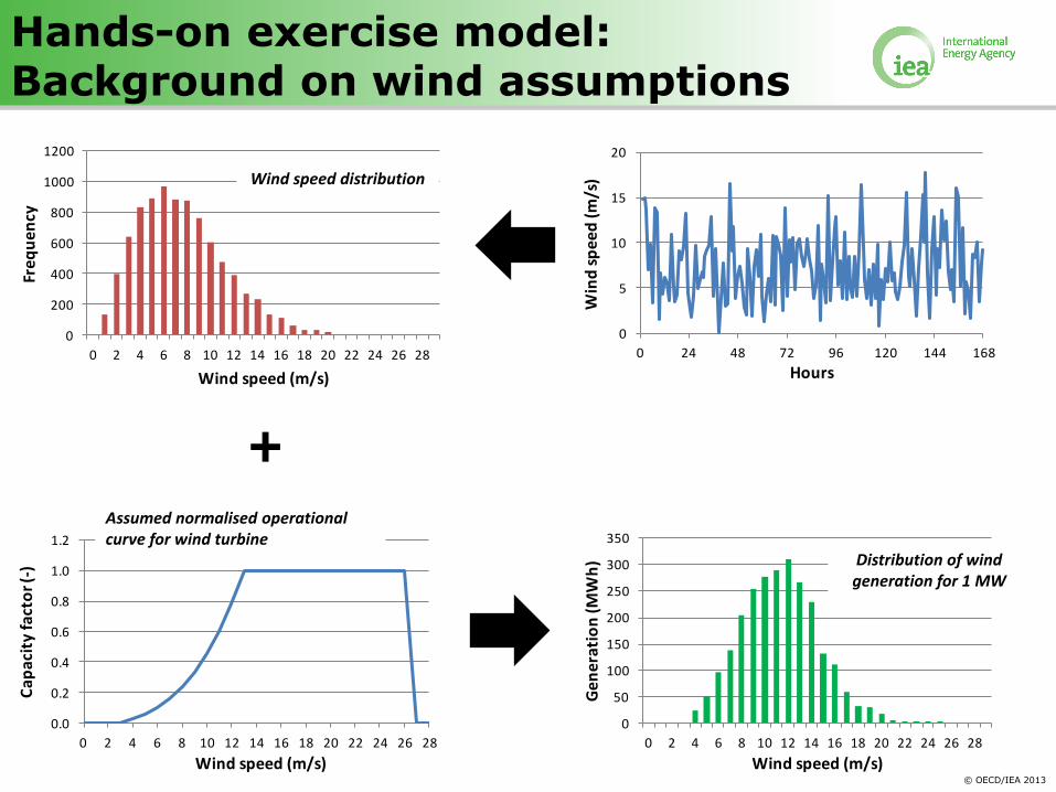
Hands-on exercise model: Background on wind assumptions
0
5
10
15
20
0 24 48 72 96 120 144 168
Win
d s
pe
ed
(m
/s)
Hours
0
200
400
600
800
1000
1200
0 2 4 6 8 10 12 14 16 18 20 22 24 26 28
Fre
qu
en
cy
Wind speed (m/s)
Wind speed distribution
0
50
100
150
200
250
300
350
0 2 4 6 8 10 12 14 16 18 20 22 24 26 28
Ge
ne
rati
on
(M
Wh
)
Wind speed (m/s)
Distribution of wind generation for 1 MW
Assumed normalised operational curve for wind turbine
+
© OECD/IEA 2013
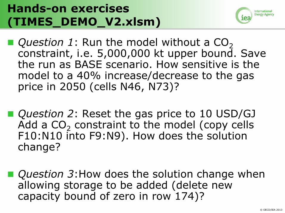
Hands-on exercises (TIMES_DEMO_V2.xlsm)
Question 1: Run the model without a CO2 constraint, i.e. 5,000,000 kt upper bound. Save the run as BASE scenario. How sensitive is the model to a 40% increase/decrease to the gas price in 2050 (cells N46, N73)?
Question 2: Reset the gas price to 10 USD/GJ Add a CO2 constraint to the model (copy cells F10:N10 into F9:N9). How does the solution change?
Question 3:How does the solution change when allowing storage to be added (delete new capacity bound of zero in row 174)?
© OECD/IEA 2013
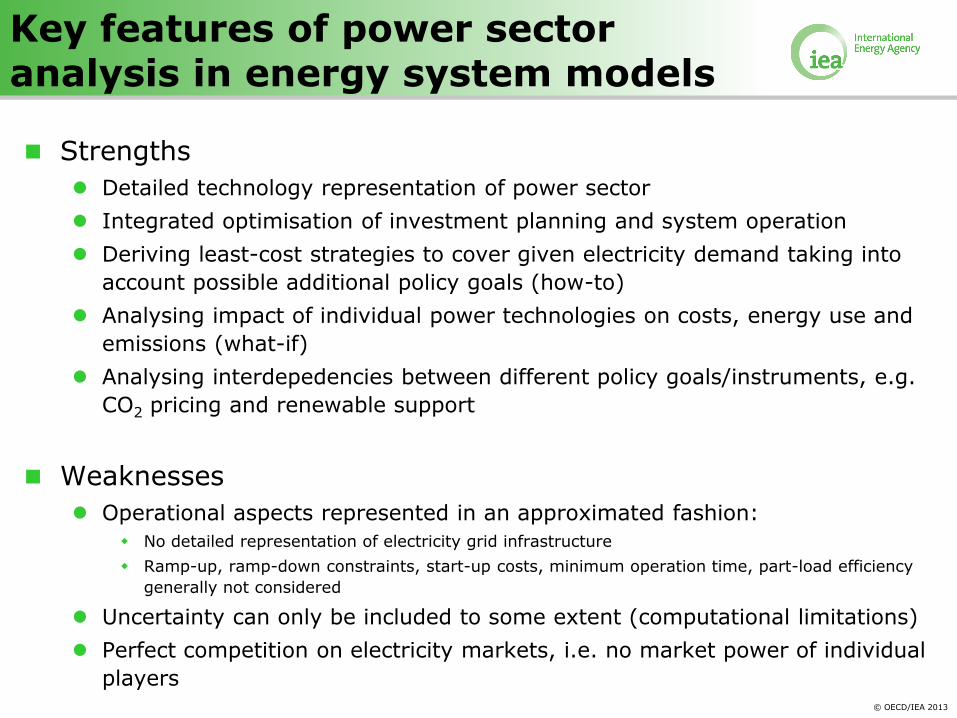
Key features of power sector analysis in energy system models
Strengths
Detailed technology representation of power sector
Integrated optimisation of investment planning and system operation
Deriving least-cost strategies to cover given electricity demand taking into
account possible additional policy goals (how-to)
Analysing impact of individual power technologies on costs, energy use and
emissions (what-if)
Analysing interdepedencies between different policy goals/instruments, e.g.
CO2 pricing and renewable support
Weaknesses
Operational aspects represented in an approximated fashion:
No detailed representation of electricity grid infrastructure
Ramp-up, ramp-down constraints, start-up costs, minimum operation time, part-load efficiency
generally not considered
Uncertainty can only be included to some extent (computational limitations)
Perfect competition on electricity markets, i.e. no market power of individual
players