ENEE759K/CMSC751: Parallel Algorithmics, Spring 2012

Time and Location • MW 2:00-3:15. JMP 2202

Instructor: Dr. U. Vishkin • E-mail: vishkin@umd.edu • Office hours: M 5:00-6:00 (by appointment) at AVW 2365

TA • James Edwards, jedward5@umd.edu

Home Page• http://www.umiacs.umd.edu/users/vishkin/TEACHING/enee759

k-s12.html

Did you get my test email? Main way for course announcements

Course GoalsIntroduction to the theory of parallel algorithms

Parallel algorithmic thinking obtaining good speed-ups over best serial algorithm. Class presentations & dry HW Study the theory of parallel algorithms; design & asymptotic analysis of parallel algorithms.

Programming reduce to practice. Why?

Hard speedups on real HW (XMT) 1. Improved understanding. 2. YOU can do it: (i) in course assignments. (ii) for most advanced algorithms studied.

Examination: (still open) CS&E research question Will the emerging ``Billion-transistor-per-chip'' era provide a way for building a truly general-purpose parallel computer system on-chip?

Focus Single program completion time.

(Throughput is important, but is a different challenge)

How to Think Algorithmically in Parallel?

Uzi Vishkin

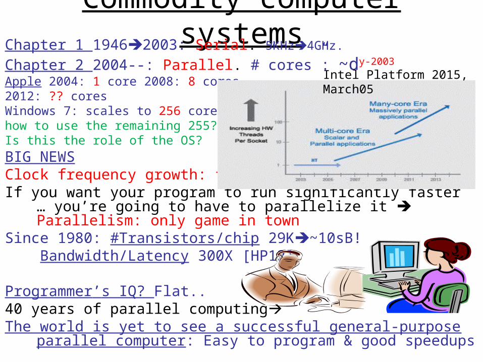
Commodity computer systemsChapter 1 19462003: Serial. 5KHz4GHz.

Chapter 2 2004--: Parallel. #”cores”: ~dy-2003 Apple 2004: 1 core 2008: 8 cores2012: ?? coresWindows 7: scales to 256 cores…how to use the remaining 255? Is this the role of the OS?

BIG NEWSClock frequency growth: flat. If you want your program to run significantly faster … you’re going

to have to parallelize it Parallelism: only game in townSince 1980: #Transistors/chip 29K~10sB! Bandwidth/Latency 300X [HP12]

Programmer’s IQ? Flat..40 years of parallel computingThe world is yet to see a successful general-purpose parallel

computer: Easy to program & good speedups

Intel Platform 2015, March05

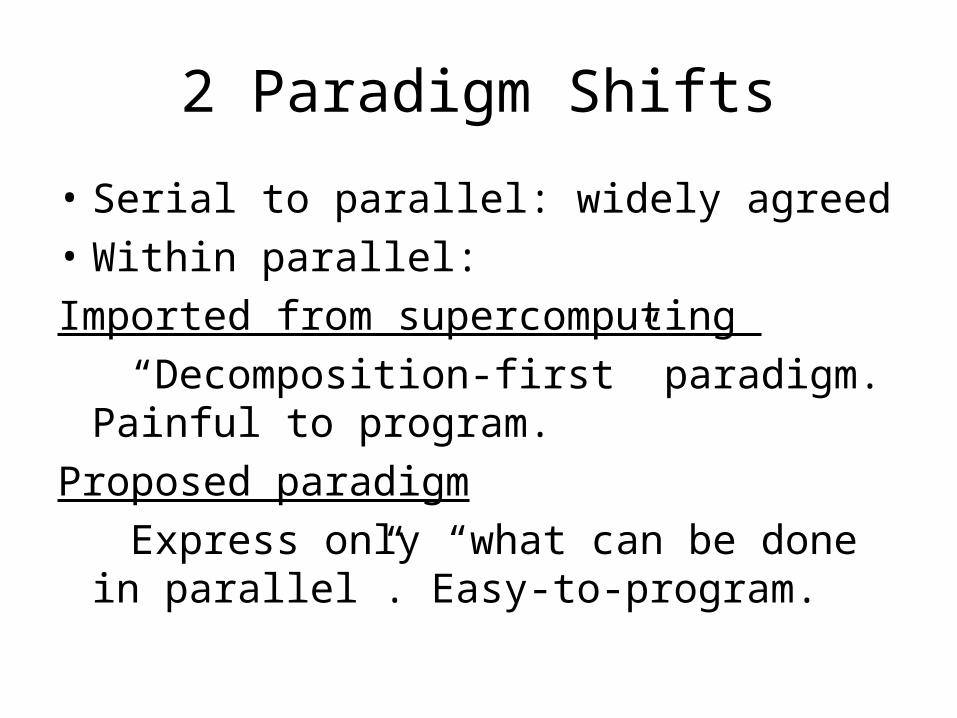
2 Paradigm Shifts

• Serial to parallel: widely agreed

• Within parallel:

Imported from supercomputing

“Decomposition-first” paradigm. Painful to program.

Proposed paradigm

Express only “what can be done in parallel”. Easy-to-program.

Abstractions in CS(i) Any particular word of an indefinitely large memory is

immediately available

(ii) A uniprocessor is serving the task that the user is currently working on exclusively.

(i) abstracts away a hierarchy of memories, each has greater capacity, but slower access time, than the preceding one. (ii) abstracts way: virtual file systems that can be implemented in local storage or a local or global network, the (whole) web, and other tasks that may be concurrently using the same computer system. These abstractions have improved productivity of programmers and other users, and contributed towards broadening participation in computing.  

• The proposed addition to this consensus is as follows. That an indefinitely large number of operations available for concurrent execution executes immediately.

The Pain of Parallel Programming• Parallel programming is currently too difficult:- To many users programming existing parallel computers is “as

intimidating and time consuming as programming in assembly language” [NSF Blue-Ribbon Panel on Cyberinfrastructure].

- AMD/Intel: “Need PhD in CS to program today’s multicores”.

• The real problem: Parallel architectures built using the following “methodology”: build-first figure-out-how-to-program-later. [J. Hennessy: “Many of the early ideas were motivated by observations of what was easy to implement in the hardware rather than what was easy to use”]

• Tribal lore, parallel programming profs, DARPA HPCS Development Time study (2004-2008): “Parallel algorithms and programming for parallelism is easy.What is difficult is the programming/tuning for performance that comes after that.”

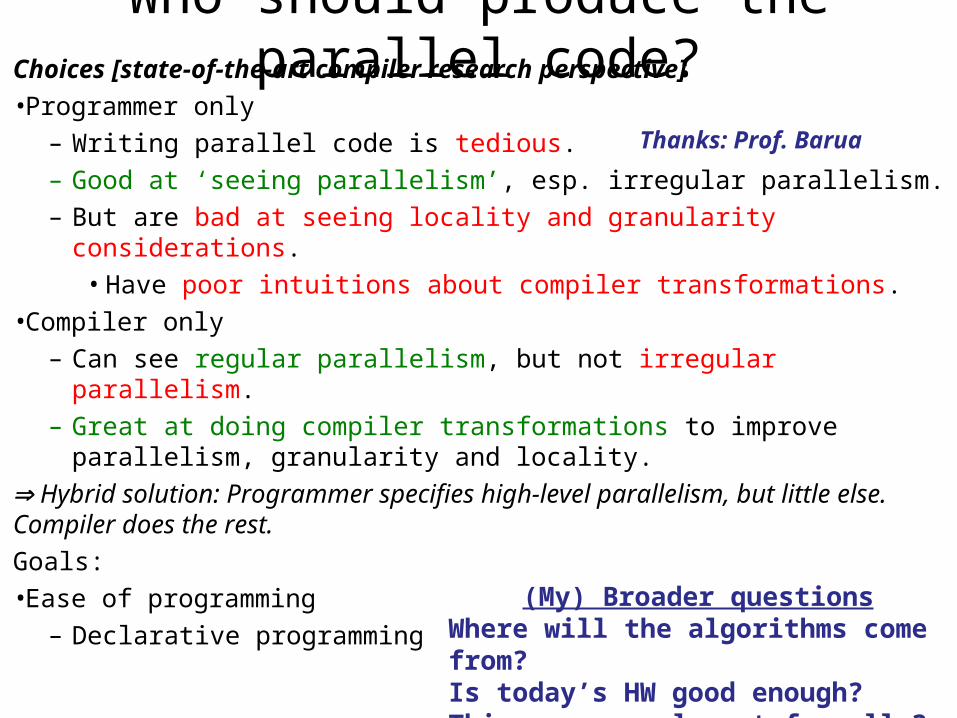
Who should produce the parallel code?Choices [state-of-the-art compiler research perspective] •Programmer only

– Writing parallel code is tedious.– Good at ‘seeing parallelism’, esp. irregular parallelism.– But are bad at seeing locality and granularity considerations.

• Have poor intuitions about compiler transformations.•Compiler only

– Can see regular parallelism, but not irregular parallelism.– Great at doing compiler transformations to improve parallelism,

granularity and locality.

Hybrid solution: Programmer specifies high-level parallelism, but little else. Compiler does the rest.

Goals:•Ease of programming

– Declarative programming

(My) Broader questionsWhere will the algorithms come from? Is today’s HW good enough?This course relevant for all 3 questions

Thanks: Prof. Barua

Welcome to today’s impasse/denial“All” vendors committed to multi-cores. Yet, their architecture and

how to program them for single program completion time not clear/stable/robust

The software spiral (HW improvements SW imp HW imp) – growth engine for IT (A. Grove, Intel); Alas, now broken!

SW vendors avoid investment in long-term SW development since may bet on the wrong horse. Impasse bad for business

Diminished competition among HW vendors.

Parallel programming education: Does CS&E degree mean: being trained for a 50yr career dominated by parallelism by programming yesterday’s serial computers? If no, why not same impasse?

Can teach common denominator (grad, seniors, freshmen, HS) the education enterprise has an actionable agenda!

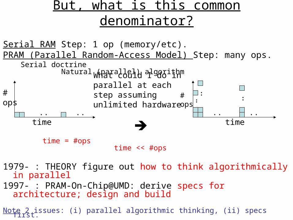
But, what is this common denominator?

Serial RAM Step: 1 op (memory/etc). PRAM (Parallel Random-Access Model) Step: many ops. Serial doctrine Natural (parallel)

algorithm

time = #ops time << #ops

1979- : THEORY figure out how to think algorithmically in parallel 1997- : PRAM-On-Chip@UMD: derive specs for architecture;

design and build

Note 2 issues: (i) parallel algorithmic thinking, (ii) specs first.

What could I do in parallel at each step assuming unlimited hardware

#ops

.. ..

.... ..

.. ..

# ops

time time

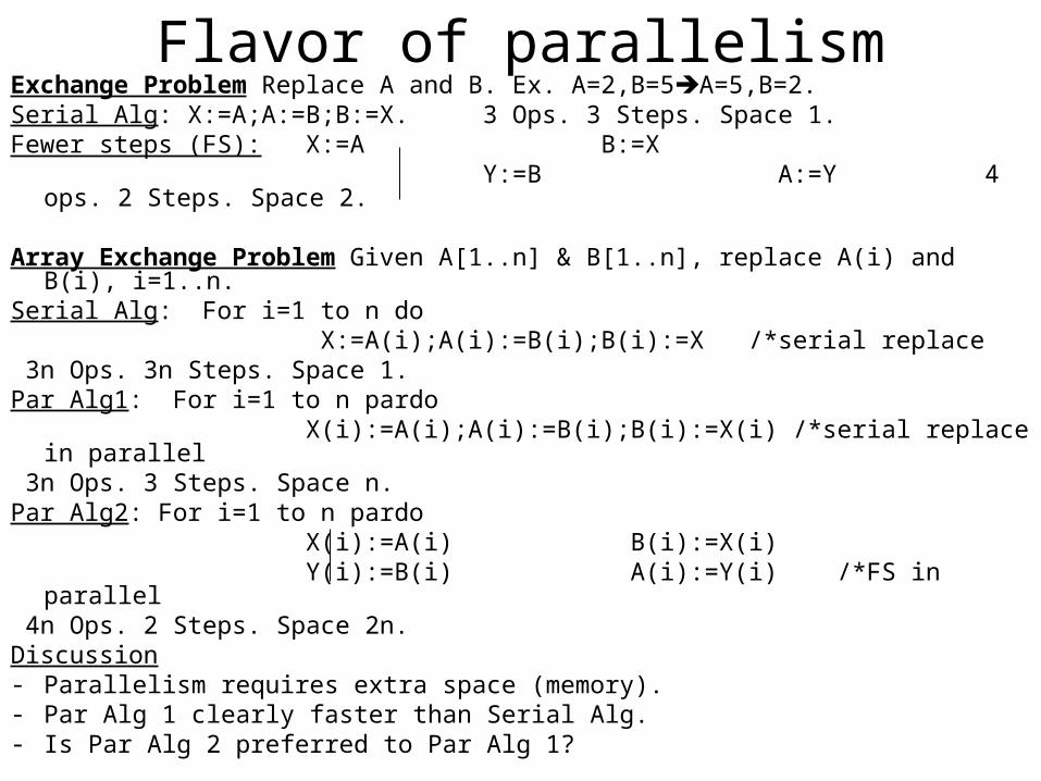
Flavor of parallelismExchange Problem Replace A and B. Ex. A=2,B=5A=5,B=2.Serial Alg: X:=A;A:=B;B:=X. 3 Ops. 3 Steps. Space 1.Fewer steps (FS): X:=A B:=X Y:=B A:=Y 4 ops. 2 Steps. Space 2.

Array Exchange Problem Given A[1..n] & B[1..n], replace A(i) and B(i), i=1..n.Serial Alg: For i=1 to n do X:=A(i);A(i):=B(i);B(i):=X /*serial replace 3n Ops. 3n Steps. Space 1.Par Alg1: For i=1 to n pardo X(i):=A(i);A(i):=B(i);B(i):=X(i) /*serial replace in parallel 3n Ops. 3 Steps. Space n.Par Alg2: For i=1 to n pardo X(i):=A(i) B(i):=X(i) Y(i):=B(i) A(i):=Y(i) /*FS in parallel 4n Ops. 2 Steps. Space 2n.Discussion - Parallelism requires extra space (memory). - Par Alg 1 clearly faster than Serial Alg. - Is Par Alg 2 preferred to Par Alg 1?

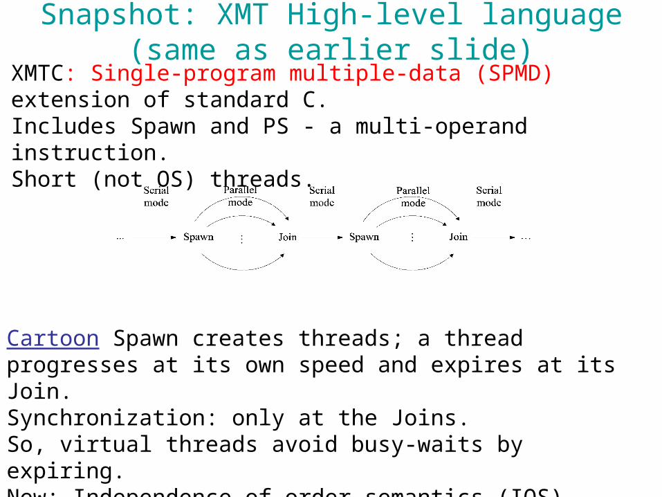
Snapshot: XMT High-level languageXMTC: Single-program multiple-data (SPMD) extension of standard C.Includes Spawn and PS - a multi-operand instruction. Short (not OS) threads.

Cartoon Spawn creates threads; a thread progresses at its own speed and expires at its Join. Synchronization: only at the Joins. So, virtual threads avoid busy-waits by expiring. New: Independence of order semantics (IOS).

Array Exchange. Pseudo-code for Par Alg1 Spawn(1,n){ X($):=A($);A($):=B($);B($):=X($) }

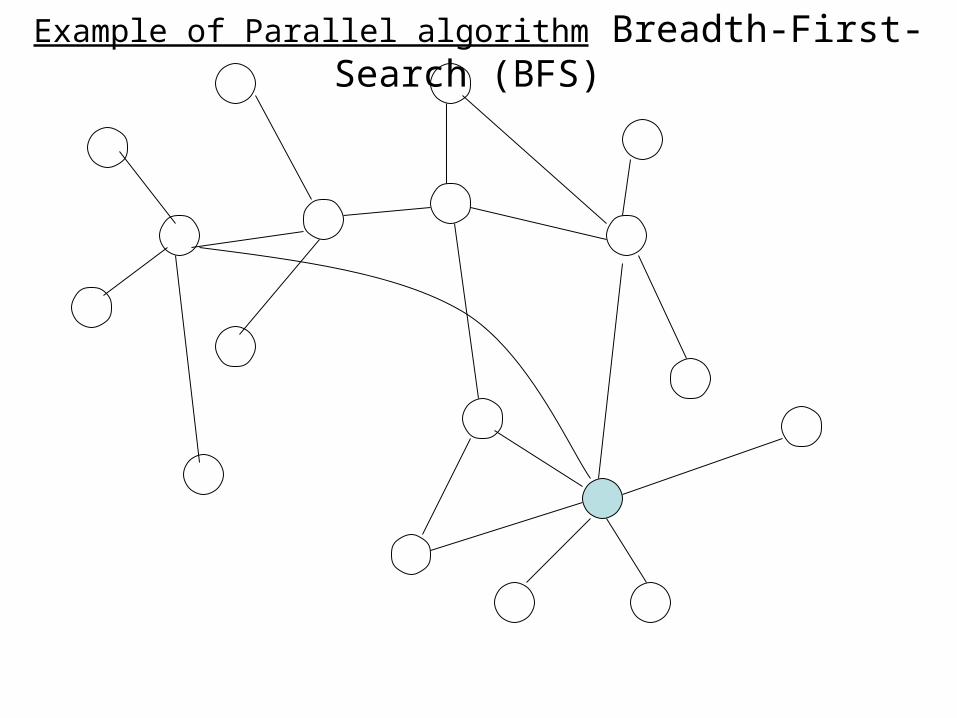
Example of Parallel algorithm Breadth-First-Search (BFS)

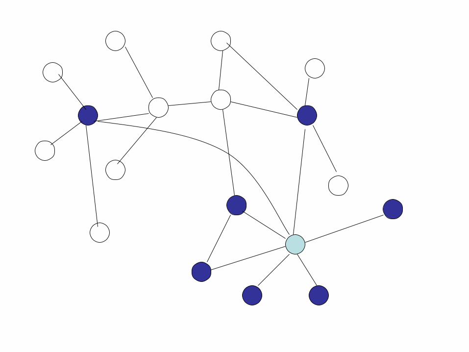
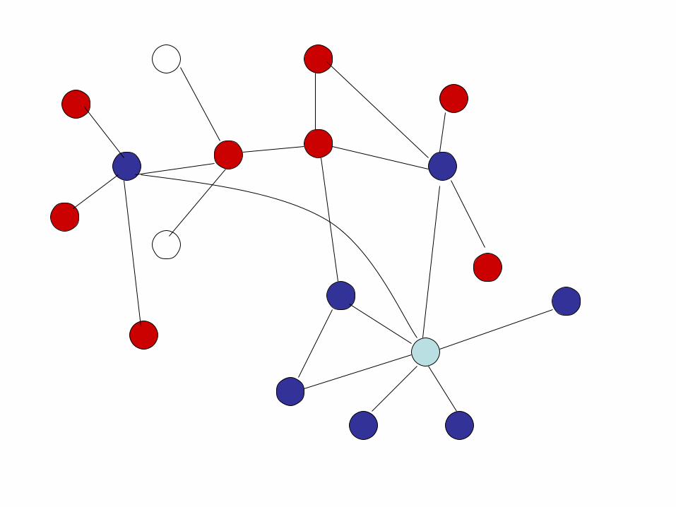
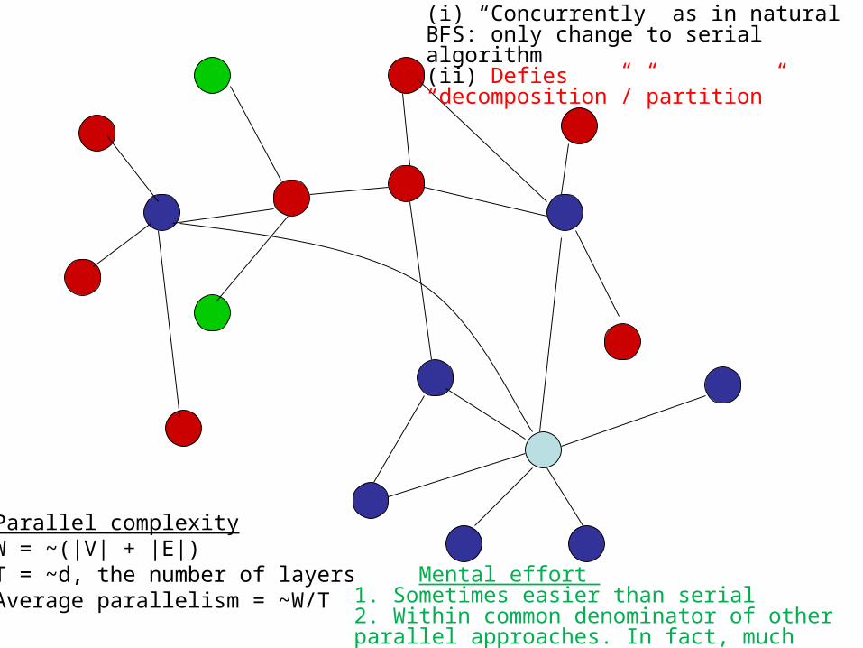
Parallel complexityW = ~(|V| + |E|)T = ~d, the number of layersAverage parallelism = ~W/T

(i) “Concurrently” as in natural BFS: only change to serial algorithm(ii) Defies “decomposition”/”partition”

Mental effort 1. Sometimes easier than serial 2. Within common denominator of other parallel approaches. In fact, much easier

1st example for denial [EduPar2011]2011 NSF/IEEE-TCPP curriculum teach BFS using OpenMP

Teaching experiment Joint F2010 UIUC/UMD class. 42 students

Good news Easy coding (since no meaningful ‘decomposition’)

Bad news None got speedup over serial on 8-proc SMP machine

BFS alg was easy but .. no good: no speedups

Speedups on 64-processor XMT 7x to 25x

Fair to compare 64 processors to 8 since <1/4 of the silicon area

Symptom of the bigger denial

‘Only problem Developers lack parallel programming skills’

Solution Education. False Teach then see that HW is the problem. Secret Nobody demands hard speedups from undergrads, but be quiet$$$

HotPAR10 performance results include BFS:XMT/GPU Speed-up same silicon area, highly parallel input: 5.4XSmall HW configuration, large diameter: 109X wrt same GPU

Discussion of BFS results

• Contrast with smartest people, Stanford’11, Nvidia’12 .. BFS on multi-cores/GPUs, again only if the diameter is small, improving on a SC’10 IBM/GaTech and 6 other recent papers, all 1st rate conferences.

BFS is bread & butter. Call the Marines each time you need

bread? Makes one wonder What is wrong with this field?!

• ‘Decree’ Random graphs = ‘reality’. In the old days: Expander graphs taught in graph design. Planar graphs were real

• Lots of parallelism more HW design freedom. E.g., GPUs get decent speedup with lots of parallelism.

But, not enough for general parallel algorithms. BFS (& max-flow): better speedups and easier programs on XMT

More Order-of-Magnitude Denial Examples 1Performance Example Parallel Max-Flow speedups vs best serial

– [HeHo, IPDPS10] <= 2.5x using best of CUDA & CPU hybrid– [CarageaV, SPAA11] <= 108.3x using XMT (ShiloachV&GoldbergTarjan)

Big effort beyond published algorithms vs normal theory-to-practice Advantage by 43X

Why max-flow example?As advanced any irregular fine-grained parallel algorithms dared on any parallel architecture

- Horizons of a computer architecture cannot only be studied using elementary algorithms [Performance, efficiency and effectiveness of a car not tested only in low gear or limited road conditions]

- Stress test for important architecture capabilities not often discussed:1.Strong scaling : Increase #processors, not problem size2.Rewarding even little amounts of algorithm parallelism with speedups

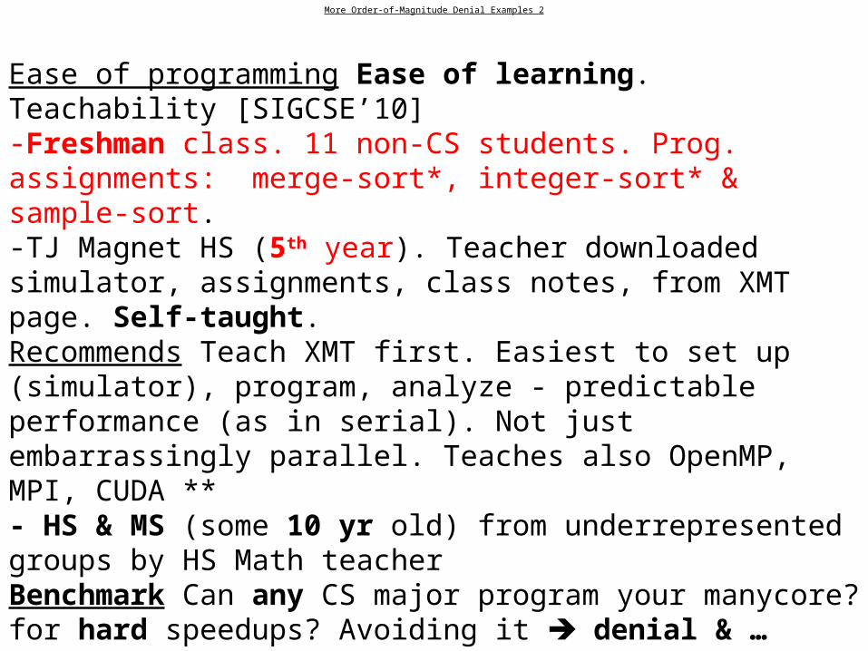
More Order-of-Magnitude Denial Examples 2

Ease of programming Ease of learning. Teachability [SIGCSE’10]-Freshman class. 11 non-CS students. Prog. assignments: merge-sort*, integer-sort* & sample-sort. -TJ Magnet HS (5th year). Teacher downloaded simulator, assignments, class notes, from XMT page. Self-taught. Recommends Teach XMT first. Easiest to set up (simulator), program, analyze - predictable performance (as in serial). Not just embarrassingly parallel. Teaches also OpenMP, MPI, CUDA **- HS & MS (some 10 yr old) from underrepresented groups by HS Math teacherBenchmark Can any CS major program your manycore? for hard speedups? Avoiding it denial & … state-of-the-artProgrammability necessary condition for success of a many core platform. Teachability necessary for that & a practical benchmark.*In Nvidia + UC Berkeley IPDPS09 research paper! **Also, keynote at CS4HS’09@CMU + interview with teacher

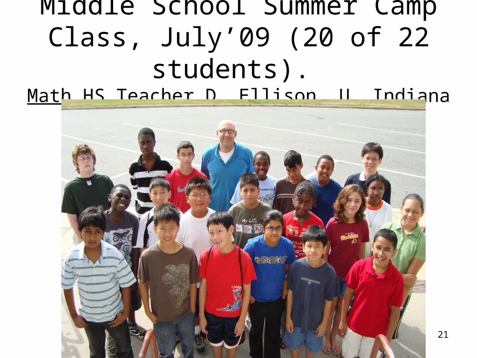
Middle School Summer Camp Class, July’09 (20 of 22 students). Math HS Teacher D. Ellison, U. Indiana

21

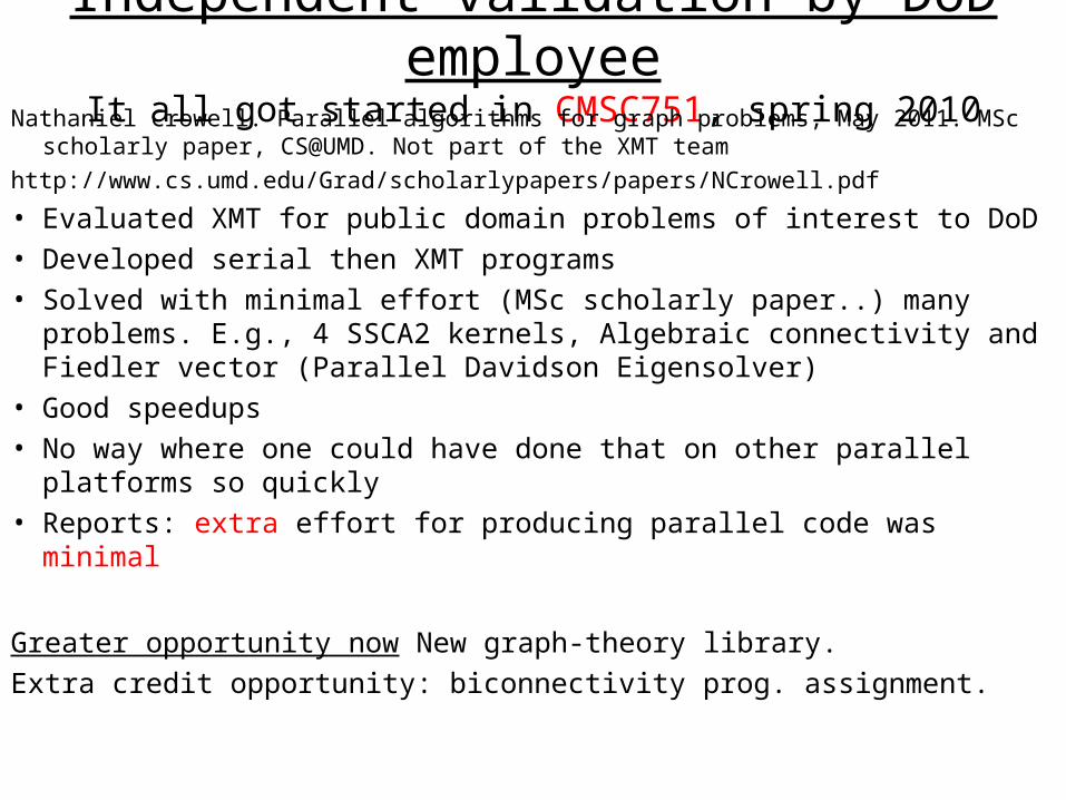
Independent validation by DoD employeeIt all got started in CMSC751, spring 2010

Nathaniel Crowell. Parallel algorithms for graph problems, May 2011. MSc scholarly paper, CS@UMD. Not part of the XMT team

http://www.cs.umd.edu/Grad/scholarlypapers/papers/NCrowell.pdf

• Evaluated XMT for public domain problems of interest to DoD • Developed serial then XMT programs • Solved with minimal effort (MSc scholarly paper..) many problems. E.g.,

4 SSCA2 kernels, Algebraic connectivity and Fiedler vector (Parallel Davidson Eigensolver)

• Good speedups• No way where one could have done that on other parallel platforms so

quickly• Reports: extra effort for producing parallel code was minimal

Greater opportunity now New graph-theory library.

Extra credit opportunity: biconnectivity prog. assignment.

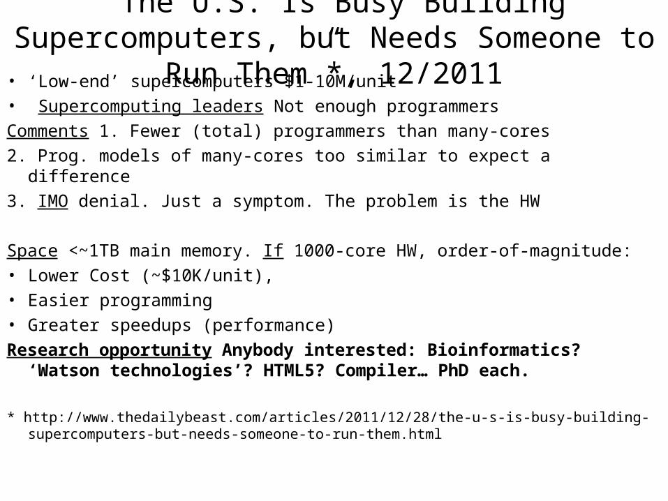
“The U.S. Is Busy Building Supercomputers, but Needs Someone to Run Them”*, 12/2011

• ‘Low-end’ supercomputers $1-10M/unit • Supercomputing leaders Not enough programmers

Comments 1. Fewer (total) programmers than many-cores

2. Prog. models of many-cores too similar to expect a difference

3. IMO denial. Just a symptom. The problem is the HW

Space <~1TB main memory. If 1000-core HW, order-of-magnitude: • Lower Cost (~$10K/unit), • Easier programming• Greater speedups (performance)

Research opportunity Anybody interested: Bioinformatics? ‘Watson technologies’? HTML5? Compiler… PhD each.

* http://www.thedailybeast.com/articles/2011/12/28/the-u-s-is-busy-building-supercomputers-but-needs-someone-to-run-them.html

NeedA general-purpose parallel computer framework [“successor to the

Pentium for the multi-core era”] that:(i) is easy to program; (ii) gives good performance with any amount of parallelism

provided by the algorithm; namely, up- and down-scalability including backwards compatibility on serial code;

(iii) supports application programming (VHDL/Verilog, OpenGL, MATLAB) and performance programming; and

(iv) fits current chip technology and scales with it.(in particular: strong speed-ups for single-task completion time)

Main Point of talk: PRAM-On-Chip@UMD is addressing (i)-(iv).

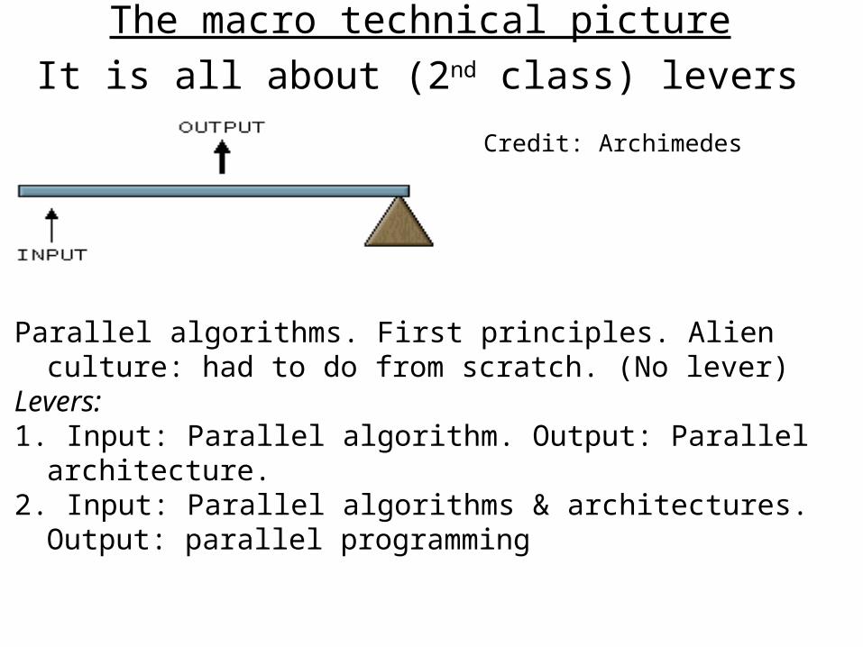
The macro technical picture

It is all about (2nd class) levers Credit: Archimedes

Parallel algorithms. First principles. Alien culture: had to do from scratch. (No lever)

Levers:1. Input: Parallel algorithm. Output: Parallel architecture.2. Input: Parallel algorithms & architectures. Output: parallel

programming

The PRAM Rollercoaster ride

Late 1970’s Theory work beganUP Won the battle of ideas on parallel algorithmic thinking.

No silver or bronze!Model of choice in all theory/algorithms communities. 1988-90: Big

chapters in standard algorithms textbooks.DOWN FCRC’93: “PRAM is not feasible”. [‘93+ despair no

good alternative! Where vendors expect good enough alternatives to come from now?]; Device changed it all:

UP Highlights: eXplicit-multi-threaded (XMT) FPGA-prototype computer (not simulator), SPAA’07,CF’08; 90nm ASIC tape-outs: int. network, HotI’07, XMT. # on-chip transistors

How come? crash “course” on parallel computingHow much processors-to-memories bandwidth?If enough: Ideal Programming Model (PRAM)If limited: Programming difficulties

The eXplicit MultiThreading (XMT) Easy-To-Program Parallel Computer

www.umiacs.umd.edu/users/vishkin/XMT

The XMT Overall Design Challenge

Spectrum of Explicit Multi-Threading (XMT) Framework• Algorithms −− > architecture −− > implementation.• XMT: strategic design point for fine-grained parallelism• New elements are added only where needed

Attributes• Holistic: A variety of subtle problems across different domains

must be addressed:• Understand and address each at its correct level of abstraction

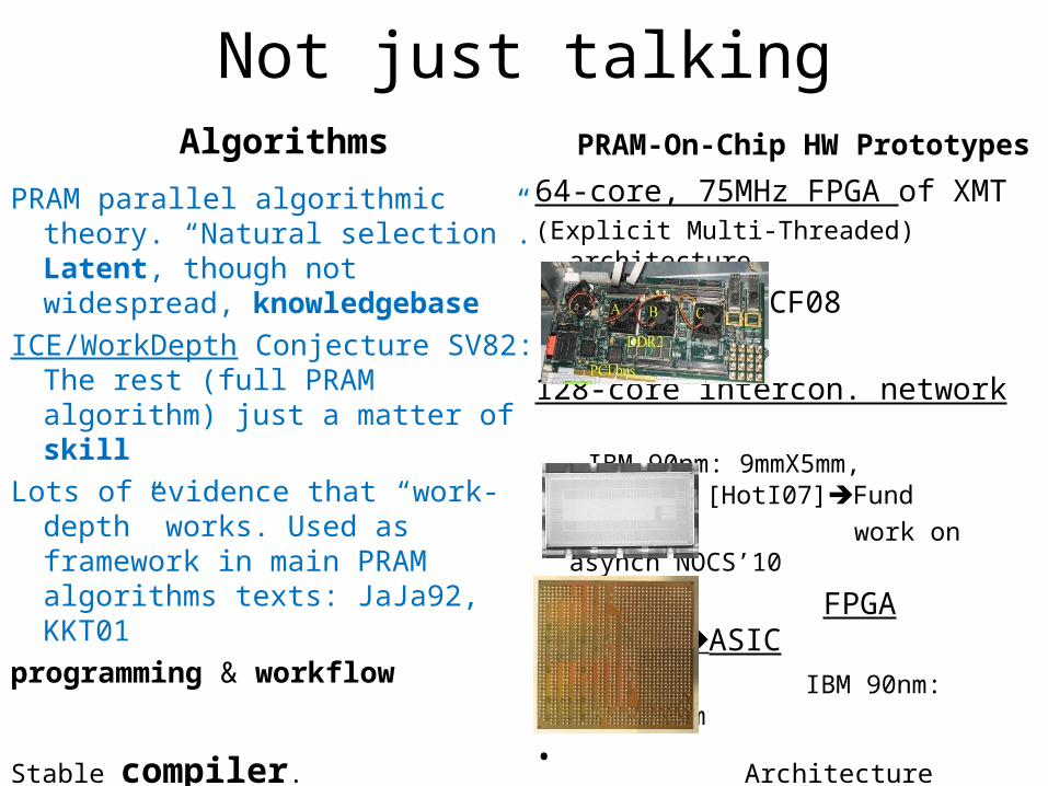
Not just talkingAlgorithms

PRAM parallel algorithmic theory. “Natural selection”. Latent, though not widespread, knowledgebase

ICE/WorkDepth Conjecture SV82: The rest (full PRAM algorithm) just a matter of skill

Lots of evidence that “work-depth” works. Used as framework in main PRAM algorithms texts: JaJa92, KKT01

programming & workflow

PRAM-On-Chip HW Prototypes

64-core, 75MHz FPGA of XMT(Explicit Multi-Threaded) architecture

SPAA98..CF08

128-core intercon. network IBM 90nm: 9mmX5mm,

400 MHz [HotI07]Fund

work on asynch NOCS’10

• FPGA designASIC • IBM 90nm: 10mmX10mm

•

Stable compiler. Architecture scales to 1000+ cores on-chip

Naming Contest for New Computer (2007)

Paraleap

chosen out of ~6000 submissions

Single (hard working) person (X. Wen) completed synthesizable Verilog description AND the new FPGA-based XMT computer in slightly more than two years. No prior design experience. Attests to: basic simplicity of the XMT architecture faster time to market, lower implementation cost.

Experience with High School Students, Fall’07

1-day parallel algorithms tutorial to 12 HS students. Some (2 10th graders) managed 8 programming assignments, including 5 of the 6 in the grad course. Only help: 1 office hour/week by undergrad TA. No school credit. Part of a computer club after 8 periods/day.

One of these 10th graders: “I tried to work on parallel machines at school, but it was no fun: I had to program around their engineering. With XMT, I could focus on solving the problem that I had to solve.”

Software releaseAllows to use your own computer for programming on an XMT environment and experimenting with it, including:(i)Cycle-accurate simulator of the XMT machine(ii)Compiler from XMTC to that machine

Also provided, extensive material for teaching or self-studying parallelism, including(i)Tutorial + manual for XMTC (150 pages)(ii)Classnotes on parallel algorithms (100 pages)(iii)Video recording of 9/15/07 HS tutorial (300 minutes)

Next Major Objective

Industry-grade chip and production quality compiler. Requires 10X in funding.

Current ParticipantsGrad students: James Edwards, Beliz Saybasili, Alex Tzannes*. Recent grads:

Aydin Balkan, George Caragea, Mike Horak, Fuat Keceli, Xingzhi Wen• Industry design experts (pro-bono).• Rajeev Barua, Compiler. Co-advisor X2. NSF grant.• Gang Qu, VLSI and Power. Co-advisor.• Steve Nowick, Columbia U., Asynch computing. Co-advisor. NSF team

grant. • Ron Tzur, U. Colorado, K12 Education. Co-advisor. NSF seed fundingK12: Montgomery Blair Magnet HS, MD, Thomas Jefferson HS, VA, Baltimore (inner city)

Ingenuity Project Middle School 2009 Summer Camp, Montgomery County Public Schools• Marc Olano, UMBC, Computer graphics. Co-advisor.• Tali Moreshet, Swarthmore College, Power. Co-advisor.• Bernie Brooks, NIH. Co-Advisor.• Marty Peckerar, Microelectronics• Igor Smolyaninov, Electro-optics• Funding: NSF, NSA deployed XMT computer, NIH• Reinvention of Computing for Parallelism. 1st out of 49 for Maryland

Research Center of Excellence (MRCE) by USM. Not yet funded. 17 members, including UMBC, UMBI, UMSOM. Mostly applications.

* 1st place, ACM Student Research Competition, PACT, Oct 2011. Post-doc UIUC

Principled Objective of the CourseIdeal: Present an untainted view of the only truly

successful theory of parallel algorithms.Why is this easier said than done?Theory (3 dictionary definitions): * A body of theorems presenting a concise systematic

view of a subject. An unproved assumption: conjecture.FCRC’93: “PRAM infeasible” 2nd def not good enough“Success is not final, failure is not fatal: it is the courage to continue that counts” W. Churchill

Feasibility proof status: programming & real hw that scales to cutting edge technology. Involves a real computer: CF’08 PRAM is becoming feasible

Achievable: Minimally tainted view. Also promotes * to: The principles of a science or an art.

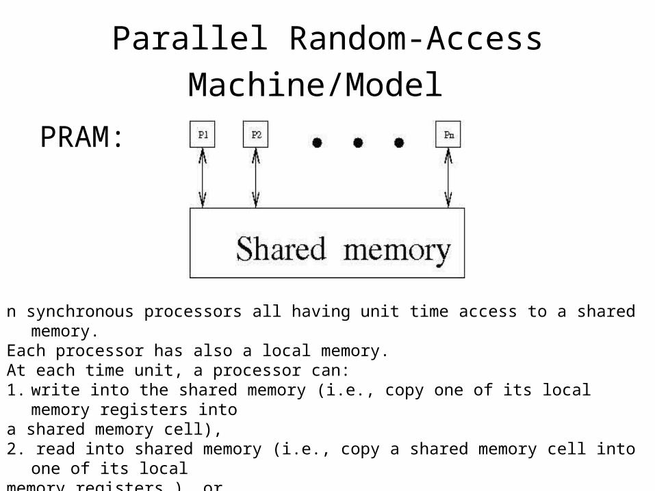
Parallel Random-Access Machine/Model

PRAM:

n synchronous processors all having unit time access to a shared memory. Each processor has also a local memory.At each time unit, a processor can:1. write into the shared memory (i.e., copy one of its local memory registers into a shared memory cell), 2. read into shared memory (i.e., copy a shared memory cell into one of its local memory registers ), or 3. do some computation with respect to its local memory.

pardo programming construct - for Pi , 1 ≤ i ≤ n pardo- A(i) := B(i)

This means The following n operations are performed concurrently: processor P1 assigns B(1) into

A(1), processor P2 assigns B(2) into A(2), ….

Modeling read&write conflicts to the same shared memory location Most common are:- exclusive-read exclusive-write (EREW) PRAM: no simultaneous access by more

than one processor to the same memory location for read or write purposes- concurrent-read exclusive-write (CREW) PRAM: concurrent access for reads but not

for writes- concurrent-read concurrent-write (CRCW allows concurrent access for both reads

and writes. We shall assume that in a concurrent-write model, an arbitrary processor among the processors attempting to write into a common memory location, succeeds. This is called the Arbitrary CRCW rule.

There are two alternative CRCW rules: (i) Priority CRCW: the smallest numbered, among the processors attempting to write into a common memory location, actually succeeds. (ii) Common CRCW: allows concurrent writes only when all the processors attempting to write into a common memory location are trying to write the same value.

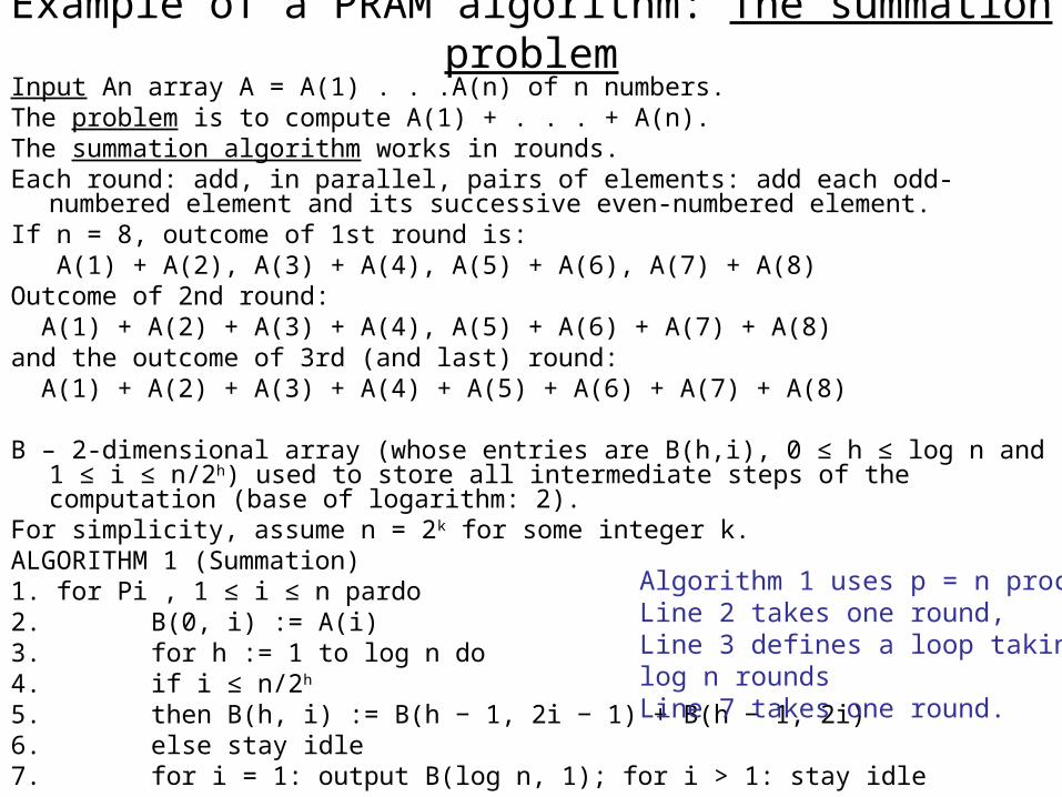
Example of a PRAM algorithm: The summation problemInput An array A = A(1) . . .A(n) of n numbers.The problem is to compute A(1) + . . . + A(n).The summation algorithm works in rounds. Each round: add, in parallel, pairs of elements: add each odd-numbered element and its

successive even-numbered element.If n = 8, outcome of 1st round is: A(1) + A(2), A(3) + A(4), A(5) + A(6), A(7) + A(8)Outcome of 2nd round: A(1) + A(2) + A(3) + A(4), A(5) + A(6) + A(7) + A(8)and the outcome of 3rd (and last) round: A(1) + A(2) + A(3) + A(4) + A(5) + A(6) + A(7) + A(8)

B – 2-dimensional array (whose entries are B(h,i), 0 ≤ h ≤ log n and 1 ≤ i ≤ n/2h) used to store all intermediate steps of the computation (base of logarithm: 2).

For simplicity, assume n = 2k for some integer k.ALGORITHM 1 (Summation)1. for Pi , 1 ≤ i ≤ n pardo2. B(0, i) := A(i)3. for h := 1 to log n do4. if i ≤ n/2h

5. then B(h, i) := B(h − 1, 2i − 1) + B(h − 1, 2i)6. else stay idle7. for i = 1: output B(log n, 1); for i > 1: stay idle

Algorithm 1 uses p = n processors. Line 2 takes one round, Line 3 defines a loop taking log n roundsLine 7 takes one round.

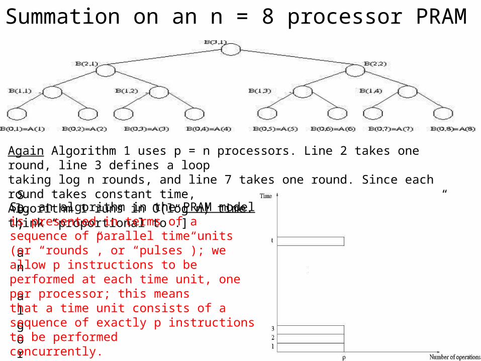
Summation on an n = 8 processor PRAM

Again Algorithm 1 uses p = n processors. Line 2 takes one round, line 3 defines a looptaking log n rounds, and line 7 takes one round. Since each round takes constant time,Algorithm 1 runs in O(log n) time. [When you see O (“big Oh”), think “proportional to”.]

So, an algorithm in the PRAM modelis presented in terms of a sequence of parallel time units (or “rounds”, or “pulses”); weallow p instructions to be performed at each time unit, one per processor; this meansthat a time unit consists of a sequence of exactly p instructions to be performedconcurrently.

So, an algorithm in the PRAM modelis presented in terms of a sequence of parallel time units (or “rounds”, or “pulses”); weallow p instructions to be performed at each time unit, one per processor; this meansthat a time unit consists of a sequence of exactly p instructions to be performedconcurrently.

Work-Depth presentation of algorithms

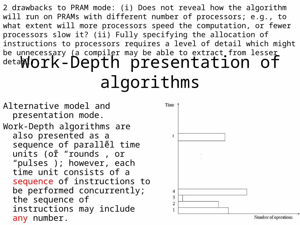
Alternative model and presentation mode.

Work-Depth algorithms are also presented as a sequence of parallel time units (or “rounds”, or “pulses”); however, each time unit consists of a sequence of instructions to be performed concurrently; the sequence of instructions may include any number.

2 drawbacks to PRAM mode: (i) Does not reveal how the algorithm will run on PRAMs with different number of processors; e.g., to what extent will more processors speed the computation, or fewer processors slow it? (ii) Fully specifying the allocation of instructions to processors requires a level of detail which might be unnecessary (a compiler may be able to extract from lesser detail)

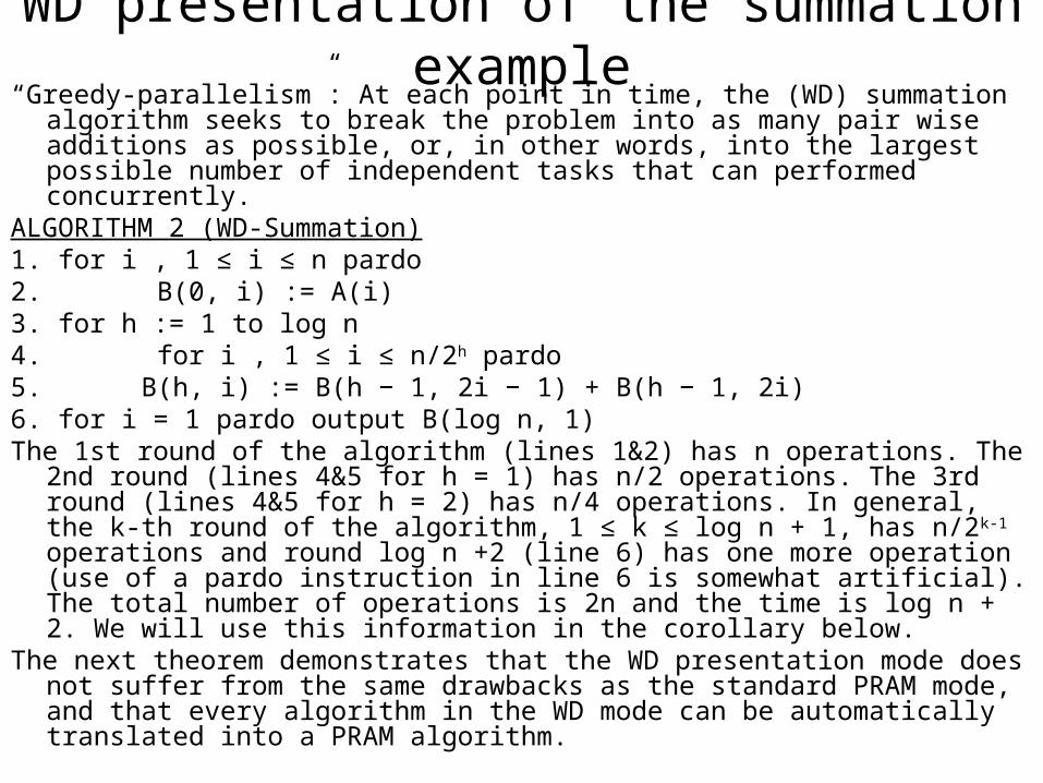
WD presentation of the summation example“Greedy-parallelism”: At each point in time, the (WD) summation algorithm

seeks to break the problem into as many pair wise additions as possible, or, in other words, into the largest possible number of independent tasks that can performed concurrently.

ALGORITHM 2 (WD-Summation)1. for i , 1 ≤ i ≤ n pardo2. B(0, i) := A(i)3. for h := 1 to log n4. for i , 1 ≤ i ≤ n/2h pardo5. B(h, i) := B(h − 1, 2i − 1) + B(h − 1, 2i)6. for i = 1 pardo output B(log n, 1)The 1st round of the algorithm (lines 1&2) has n operations. The 2nd round

(lines 4&5 for h = 1) has n/2 operations. The 3rd round (lines 4&5 for h = 2) has n/4 operations. In general, the k-th round of the algorithm, 1 ≤ k ≤ log n + 1, has n/2k-1 operations and round log n +2 (line 6) has one more operation (use of a pardo instruction in line 6 is somewhat artificial). The total number of operations is 2n and the time is log n + 2. We will use this information in the corollary below.

The next theorem demonstrates that the WD presentation mode does not suffer from the same drawbacks as the standard PRAM mode, and that every algorithm in the WD mode can be automatically translated into a PRAM algorithm.

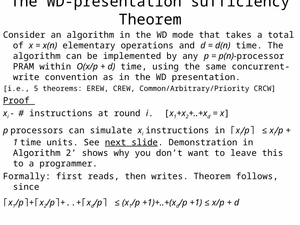
The WD-presentation sufficiency Theorem

Consider an algorithm in the WD mode that takes a total of x = x(n) elementary operations and d = d(n) time. The algorithm can be implemented by any p = p(n)-processor PRAM within O(x/p + d) time, using the same concurrent-write convention as in the WD presentation.

[i.e., 5 theorems: EREW, CREW, Common/Arbitrary/Priority CRCW]

Proof

xi - # instructions at round i. [x1+x2+..+xd = x]

p processors can simulate xi instructions in ⌈xi/p⌉ ≤ xi/p + 1 time units. See next slide. Demonstration in Algorithm 2’ shows why you don’t want to leave this to a programmer.

Formally: first reads, then writes. Theorem follows, since

⌈x1/p +⌉ ⌈x2/p +..+⌉ ⌈xd/p⌉ ≤ (x1/p +1)+..+(xd/p +1) ≤ x/p + d

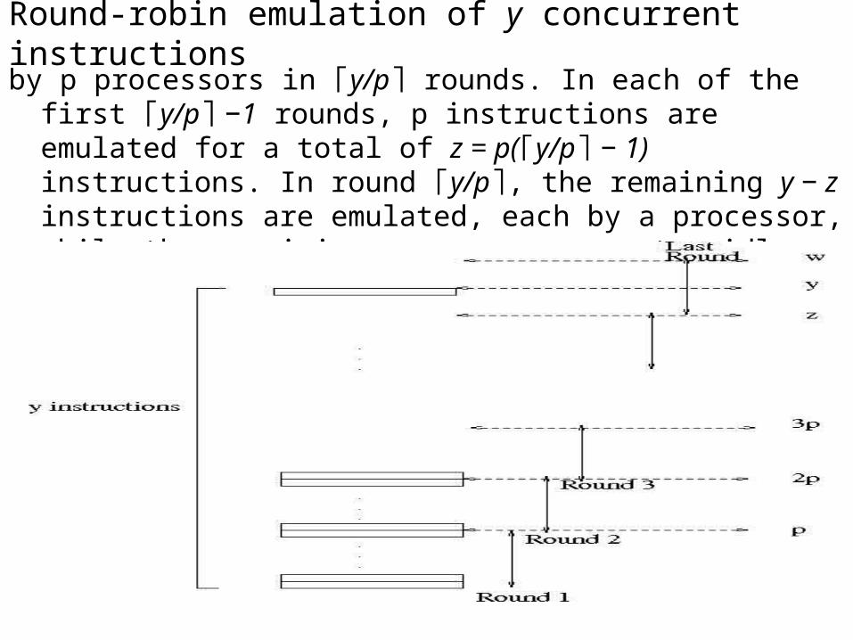
Round-robin emulation of y concurrent instructionsby p processors in ⌈y/p rounds. In each of the first ⌉ ⌈y/p⌉ −1

rounds, p instructions are emulated for a total of z = p(⌈y/p⌉ − 1) instructions. In round ⌈y/p , the remaining ⌉ y − z instructions are emulated, each by a processor, while the remaining w − y processor stay idle, where w = p⌈y/p ⌉

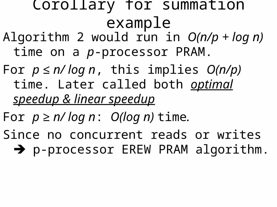
Corollary for summation example

Algorithm 2 would run in O(n/p + log n) time on a p-processor PRAM.

For p ≤ n/ log n, this implies O(n/p) time. Later called both optimal speedup & linear speedup

For p ≥ n/ log n: O(log n) time.

Since no concurrent reads or writes p-processor EREW PRAM algorithm.

ALGORITHM 2’ (Summation on a p-processor PRAM)

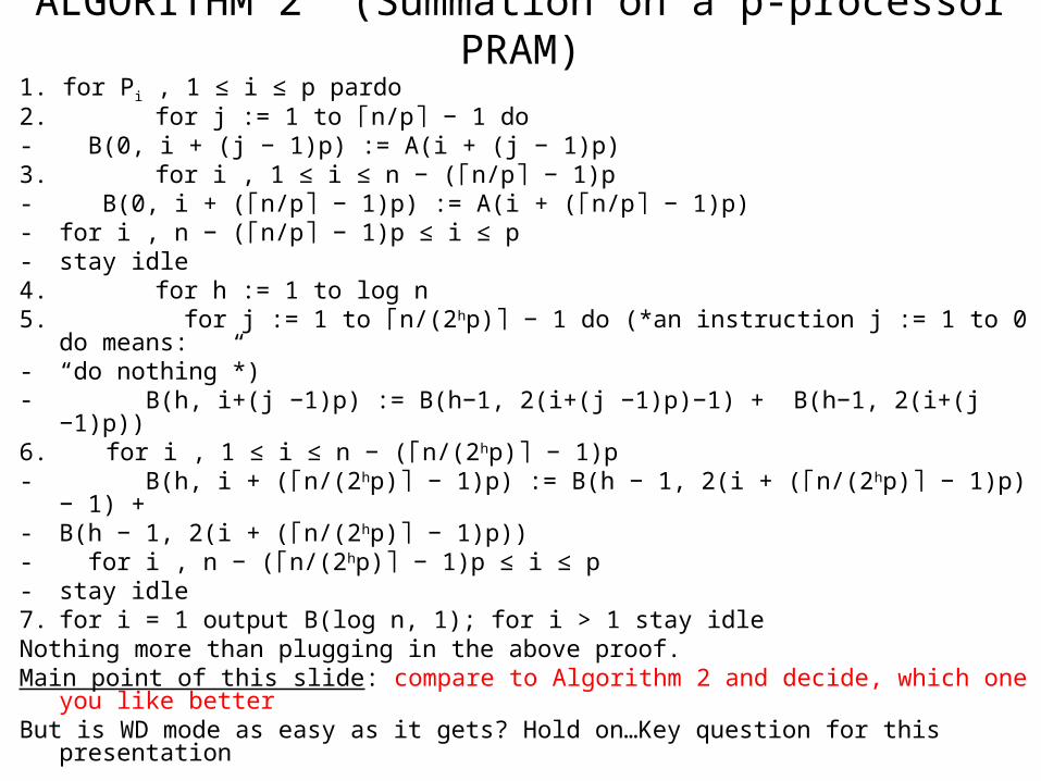
1. for Pi , 1 ≤ i ≤ p pardo2. for j := 1 to n/p − 1 do⌈ ⌉- B(0, i + (j − 1)p) := A(i + (j − 1)p)3. for i , 1 ≤ i ≤ n − ( n/p − 1)p⌈ ⌉- B(0, i + ( n/p − 1)p) := A(i + ( n/p − 1)p)⌈ ⌉ ⌈ ⌉- for i , n − ( n/p − 1)p ≤ i ≤ p⌈ ⌉- stay idle4. for h := 1 to log n5. for j := 1 to n/(2⌈ hp) − 1 do (*an instruction j := 1 to 0 do means:⌉- “do nothing”*)- B(h, i+(j −1)p) := B(h−1, 2(i+(j −1)p)−1) + B(h−1, 2(i+(j −1)p))6. for i , 1 ≤ i ≤ n − ( n/(2⌈ hp) − 1)p⌉- B(h, i + ( n/(2⌈ hp) − 1)p) := B(h − 1, 2(i + ( n/(2⌉ ⌈ hp) − 1)p) − 1) +⌉- B(h − 1, 2(i + ( n/(2⌈ hp) − 1)p))⌉- for i , n − ( n/(2⌈ hp) − 1)p ≤ i ≤ p⌉- stay idle7. for i = 1 output B(log n, 1); for i > 1 stay idleNothing more than plugging in the above proof.Main point of this slide: compare to Algorithm 2 and decide, which one you like better But is WD mode as easy as it gets? Hold on…Key question for this presentation

Measuring the performance of parallel algorithms

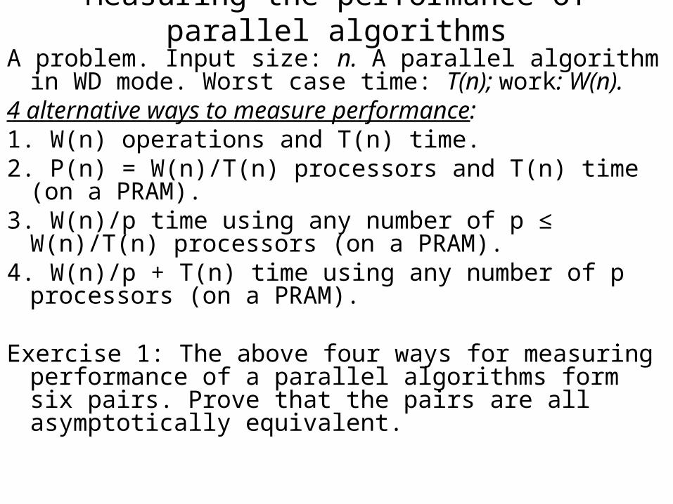
A problem. Input size: n. A parallel algorithm in WD mode. Worst case time: T(n); work: W(n).

4 alternative ways to measure performance:1. W(n) operations and T(n) time.2. P(n) = W(n)/T(n) processors and T(n) time (on a

PRAM).3. W(n)/p time using any number of p ≤ W(n)/T(n)

processors (on a PRAM).4. W(n)/p + T(n) time using any number of p processors

(on a PRAM).

Exercise 1: The above four ways for measuring performance of a parallel algorithms form six pairs. Prove that the pairs are all asymptotically equivalent.

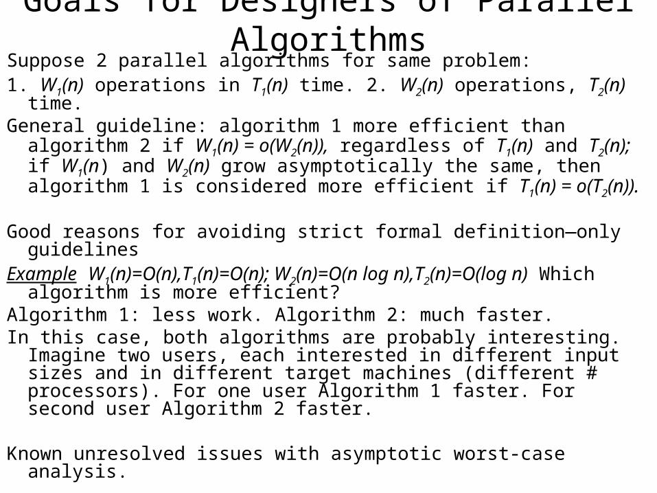
Goals for Designers of Parallel AlgorithmsSuppose 2 parallel algorithms for same problem: 1. W1(n) operations in T1(n) time. 2. W2(n) operations, T2(n) time. General guideline: algorithm 1 more efficient than algorithm 2 if

W1(n) = o(W2(n)), regardless of T1(n) and T2(n); if W1(n) and W2(n) grow asymptotically the same, then algorithm 1 is considered more efficient if T1(n) = o(T2(n)).

Good reasons for avoiding strict formal definition—only guidelinesExample W1(n)=O(n),T1(n)=O(n); W2(n)=O(n log n),T2(n)=O(log n)

Which algorithm is more efficient? Algorithm 1: less work. Algorithm 2: much faster.In this case, both algorithms are probably interesting. Imagine two

users, each interested in different input sizes and in different target machines (different # processors). For one user Algorithm 1 faster. For second user Algorithm 2 faster.

Known unresolved issues with asymptotic worst-case analysis.

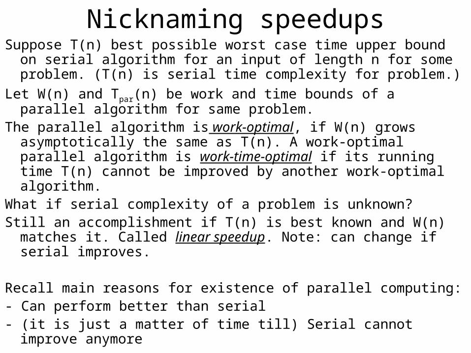
Nicknaming speedupsSuppose T(n) best possible worst case time upper bound on serial

algorithm for an input of length n for some problem. (T(n) is serial time complexity for problem.)

Let W(n) and Tpar(n) be work and time bounds of a parallel algorithm for same problem.

The parallel algorithm is work-optimal, if W(n) grows asymptotically the same as T(n). A work-optimal parallel algorithm is work-time-optimal if its running time T(n) cannot be improved by another work-optimal algorithm.

What if serial complexity of a problem is unknown?Still an accomplishment if T(n) is best known and W(n) matches it.

Called linear speedup. Note: can change if serial improves.

Recall main reasons for existence of parallel computing: - Can perform better than serial- (it is just a matter of time till) Serial cannot improve anymore

Default assumption regarding shared memory access resolution

Since all conventions represent virtual models of real machines: strongest model whose implementation cost is “still not very high”, would be practical.

Simulations results + UMD PRAM-On-Chip architecture Arbitrary CRCW

NC TheoryGood serial algorithms: poly time.

Good parallel algorithm: poly-log time, poly processors.

Was much more dominant than what’s covered here in early 1980s. Fundamental insights. Limited practicality.

In choosing abstractions: fine line between helpful and “defying gravity”

Technique: Balanced Binary Trees;

Problem: Prefix-SumsInput: Array A[1..n] of elements. Associative binary operation, denoted

, defined on the set: a (b c) = (a b) c.∗ ∗ ∗ ∗ ∗( pronounced ∗ “star”; often “sum”: addition, a common example.)The n prefix-sums of array A are:A(1)A(1) A(2)∗..A(1) A(2) .. A(i)∗ ∗ ∗..A(1) A(2) .. A(n)∗ ∗ ∗

Prefix-sums is perhaps the most heavily used routine in parallel algorithms.

ALGORITHM 1 (Prefix-sums)

1. for i , 1 ≤ i ≤ n pardo- B(0, i) := A(i)2. for h := 1 to log n3. for i , 1 ≤ i ≤ n/2h pardo- B(h, i) := B(h − 1, 2i − 1) B(h − 1, 2i)∗4. for h := log n to 05. for i even, 1 ≤ i ≤ n/2h pardo- C(h, i) := C(h + 1, i/2)6. for i = 1 pardo- C(h, 1) := B(h, 1)7. for i odd, 3 ≤ i ≤ n/2h pardo- C(h, i) := C(h + 1, (i − 1)/2) B(h, i)∗8. for i , 1 ≤ i ≤ n pardo- Output C(0, i)

Summation (as before)

C(h,i) – prefix-sum of rightmost leaf of [h,i]

}

}

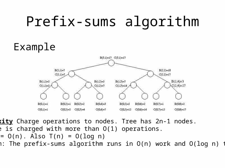
Prefix-sums algorithm

Example

Complexity Charge operations to nodes. Tree has 2n-1 nodes.No node is charged with more than O(1) operations.W(n) = O(n). Also T(n) = O(log n)Theorem: The prefix-sums algorithm runs in O(n) work and O(log n) time.

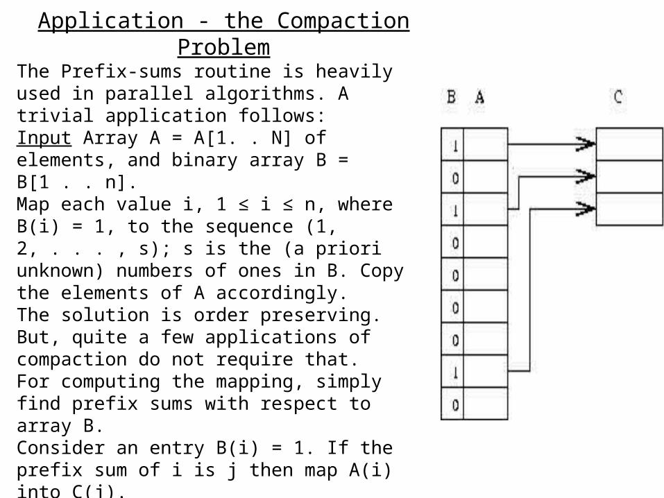
Application - the Compaction ProblemThe Prefix-sums routine is heavily used in parallel algorithms. A trivial application follows:Input Array A = A[1. . N] of elements, and binary array B = B[1 . . n].Map each value i, 1 ≤ i ≤ n, where B(i) = 1, to the sequence (1, 2, . . . , s); s is the (a priori unknown) numbers of ones in B. Copy the elements of A accordingly. The solution is order preserving. But, quite a few applications of compaction do not require that.For computing the mapping, simply find prefix sums with respect to array B. Consider an entry B(i) = 1. If the prefix sum of i is j then map A(i) into C(j). Theorem The compaction algorithm runs in O(n) work and O(log n) time.

Snapshot: XMT High-level language(same as earlier slide)

XMTC: Single-program multiple-data (SPMD) extension of standard C.Includes Spawn and PS - a multi-operand instruction. Short (not OS) threads.

Cartoon Spawn creates threads; a thread progresses at its own speed and expires at its Join. Synchronization: only at the Joins. So, virtual threads avoid busy-waits by expiring. New: Independence of order semantics (IOS).

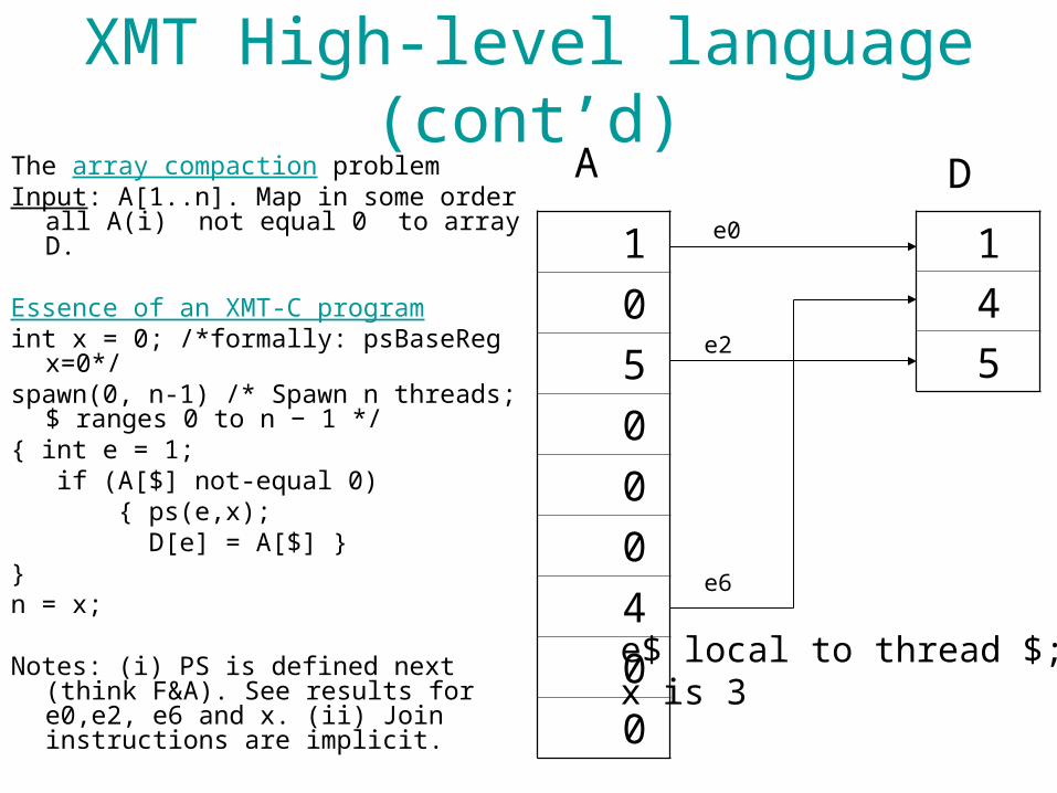
XMT High-level language (cont’d)The array compaction problemInput: A[1..n]. Map in some order all

A(i) not equal 0 to array D.

Essence of an XMT-C programint x = 0; /*formally: psBaseReg x=0*/spawn(0, n-1) /* Spawn n threads; $

ranges 0 to n − 1 */{ int e = 1; if (A[$] not-equal 0) { ps(e,x); D[e] = A[$] }}n = x;

Notes: (i) PS is defined next (think F&A). See results for e0,e2, e6 and x. (ii) Join instructions are implicit.

1

0

5

0

0

0

4

0

0

1

4

5

e0

e2

e6

A D

e$ local to thread $;x is 3

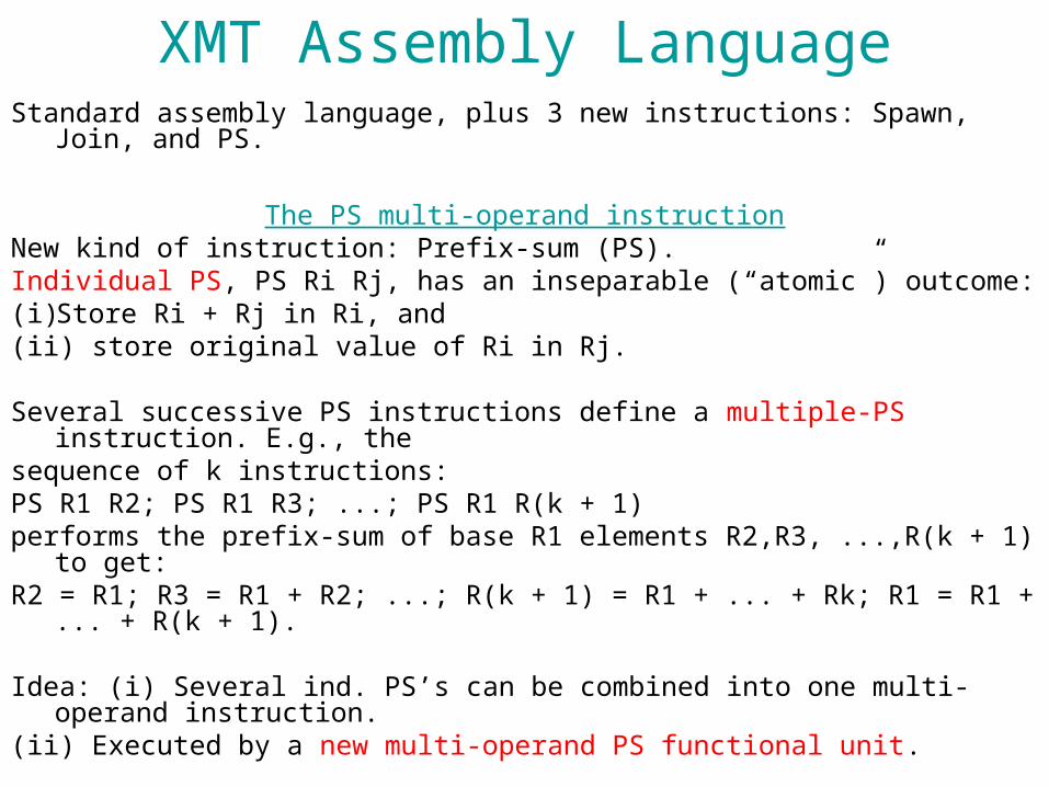
XMT Assembly LanguageStandard assembly language, plus 3 new instructions: Spawn, Join, and PS.

The PS multi-operand instructionNew kind of instruction: Prefix-sum (PS).Individual PS, PS Ri Rj, has an inseparable (“atomic”) outcome: (i) Store Ri + Rj in Ri, and (ii) store original value of Ri in Rj.

Several successive PS instructions define a multiple-PS instruction. E.g., the sequence of k instructions:PS R1 R2; PS R1 R3; ...; PS R1 R(k + 1)performs the prefix-sum of base R1 elements R2,R3, ...,R(k + 1) to get: R2 = R1; R3 = R1 + R2; ...; R(k + 1) = R1 + ... + Rk; R1 = R1 + ... + R(k + 1).

Idea: (i) Several ind. PS’s can be combined into one multi-operand instruction.(ii) Executed by a new multi-operand PS functional unit.

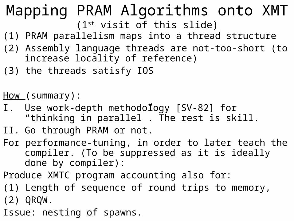
Mapping PRAM Algorithms onto XMT(1st visit of this slide)

(1) PRAM parallelism maps into a thread structure(2) Assembly language threads are not-too-short (to increase

locality of reference)(3) the threads satisfy IOS

How (summary):I. Use work-depth methodology [SV-82] for “thinking in

parallel”. The rest is skill. II. Go through PRAM or not. For performance-tuning, in order to later teach the compiler. (To

be suppressed as it is ideally done by compiler):Produce XMTC program accounting also for: (1) Length of sequence of round trips to memory,(2) QRQW. Issue: nesting of spawns.

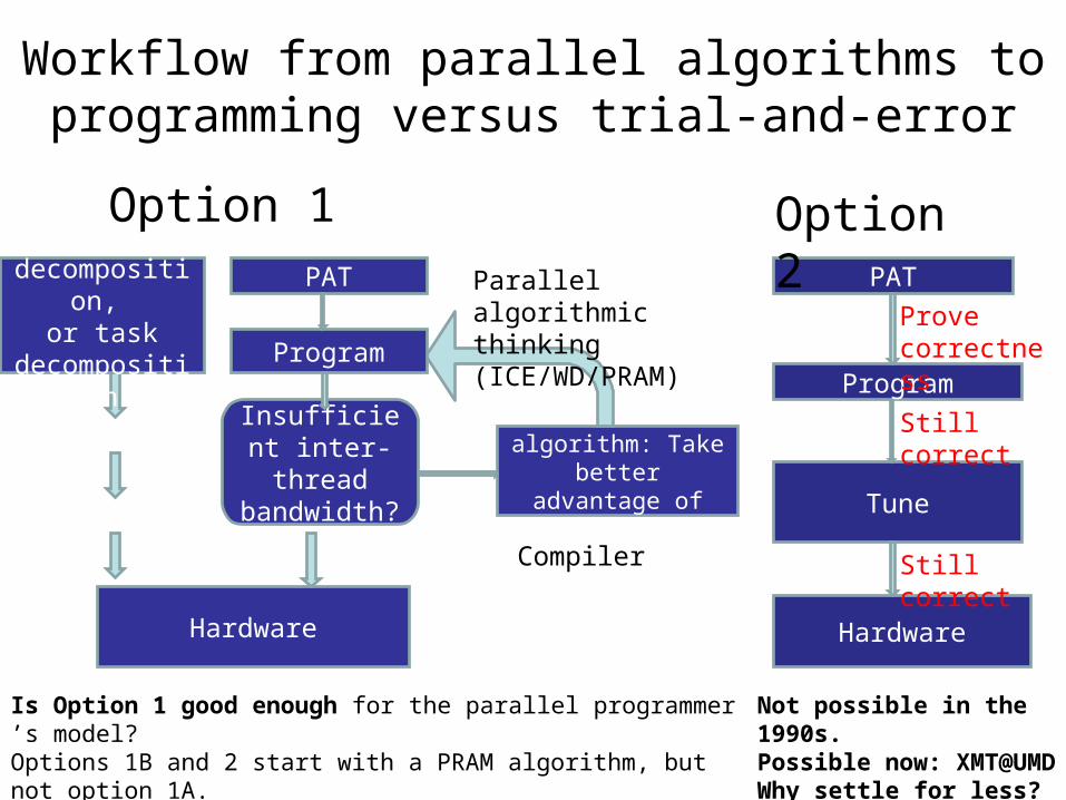
Workflow from parallel algorithms to programming versus trial-and-error

Option 1PAT

Rethink algorithm: Take better

advantage of cache

Hardware

PAT

Tune

Hardware

Option 2Parallel algorithmic thinking (ICE/WD/PRAM)

Compiler

Is Option 1 good enough for the parallel programmer’s model?Options 1B and 2 start with a PRAM algorithm, but not option 1A. Options 1A and 2 represent workflow, but not option 1B.

Not possible in the 1990s.Possible now: XMT@UMDWhy settle for less?

Insufficient inter-thread bandwidth?

Domain decomposition,

or task decomposition

ProgramProgram

Provecorrectness

Still correct

Still correct

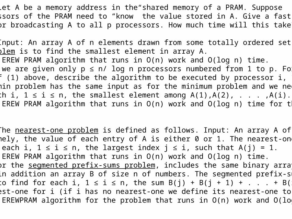
Exercise 2 Let A be a memory address in the shared memory of a PRAM. Supposeall p processors of the PRAM need to “know” the value stored in A. Give a fast EREW algorithm for broadcasting A to all p processors. How much time will this take?

Exercise 3 Input: An array A of n elements drawn from some totally ordered set. The minimum problem is to find the smallest element in array A.(1) Give an EREW PRAM algorithm that runs in O(n) work and O(log n) time.(2) Suppose we are given only p ≤ n/ log n processors numbered from 1 to p. For the algorithm of (1) above, describe the algorithm to be executed by processor i, 1 ≤ i ≤ p.The prefix-min problem has the same input as for the minimum problem and we need tofind for each i, 1 ≤ i ≤ n, the smallest element among A(1),A(2), . . . ,A(i).(3) Give an EREW PRAM algorithm that runs in O(n) work and O(log n) time for theproblem.

Exercise 4 The nearest-one problem is defined as follows. Input: An array A of size nof bits; namely, the value of each entry of A is either 0 or 1. The nearest-one problem isto find for each i, 1 ≤ i ≤ n, the largest index j ≤ i, such that A(j) = 1.(1) Give an EREW PRAM algorithm that runs in O(n) work and O(log n) time.The input for the segmented prefix-sums problem, includes the same binary array A asabove, and in addition an array B of size n of numbers. The segmented prefix-sumsproblem is to find for each i, 1 ≤ i ≤ n, the sum B(j) + B(j + 1) + . . . + B(i), where jis the nearest-one for i (if i has no nearest-one we define its nearest-one to be 1).(2) Give an EREWPRAM algorithm for the problem that runs in O(n) work and O(log n)time.

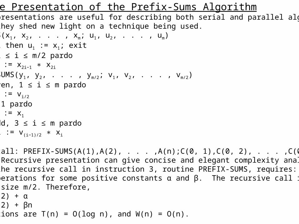
Recursive Presentation of the Prefix-Sums AlgorithmRecursive presentations are useful for describing both serial and parallel algorithms. Sometimes they shed new light on a technique being used.PREFIX-SUMS(x1, x2, . . . , xm; u1, u2, . . . , um)1. if m = 1 then u1 := x1; exit2. for i, 1 ≤ i ≤ m/2 pardo- yi := x2i−1 x∗ 2i

3. PREFIX-SUMS(y1, y2, . . . , ym/2; v1, v2, . . . , vm/2)4. for i even, 1 ≤ i ≤ m pardo- ui := vi/2

5. for i = 1 pardo- u1 := x1

6. for i odd, 3 ≤ i ≤ m pardo- ui := v(i−1)/2 x∗ i

To start, call: PREFIX-SUMS(A(1),A(2), . . . ,A(n);C(0, 1),C(0, 2), . . . ,C(0, n)).Complexity Recursive presentation can give concise and elegant complexity analysis. Excluding the recursive call in instruction 3, routine PREFIX-SUMS, requires: ≤ α time, and ≤ βm operations for some positive constants α and β. The recursive call is for a problem of size m/2. Therefore,T(n) ≤ T(n/2) + αW(n) ≤ W(n/2) + βnTheir solutions are T(n) = O(log n), and W(n) = O(n).

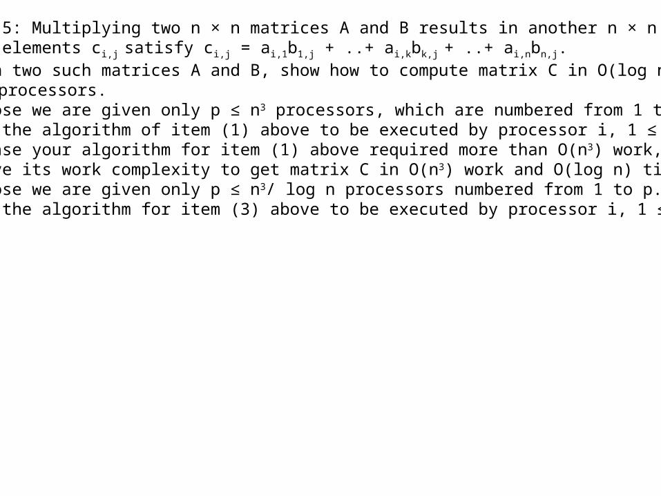
Exercise 5: Multiplying two n × n matrices A and B results in another n × n matrixC, whose elements ci,j satisfy ci,j = ai,1b1,j + ..+ ai,kbk,j + ..+ ai,nbn,j.(1) Given two such matrices A and B, show how to compute matrix C in O(log n) timeusing n3 processors.(2) Suppose we are given only p ≤ n3 processors, which are numbered from 1 to p.Describe the algorithm of item (1) above to be executed by processor i, 1 ≤ i ≤ p.(3) In case your algorithm for item (1) above required more than O(n3) work, show howto improve its work complexity to get matrix C in O(n3) work and O(log n) time.(4) Suppose we are given only p ≤ n3/ log n processors numbered from 1 to p.Describe the algorithm for item (3) above to be executed by processor i, 1 ≤ i ≤ p.

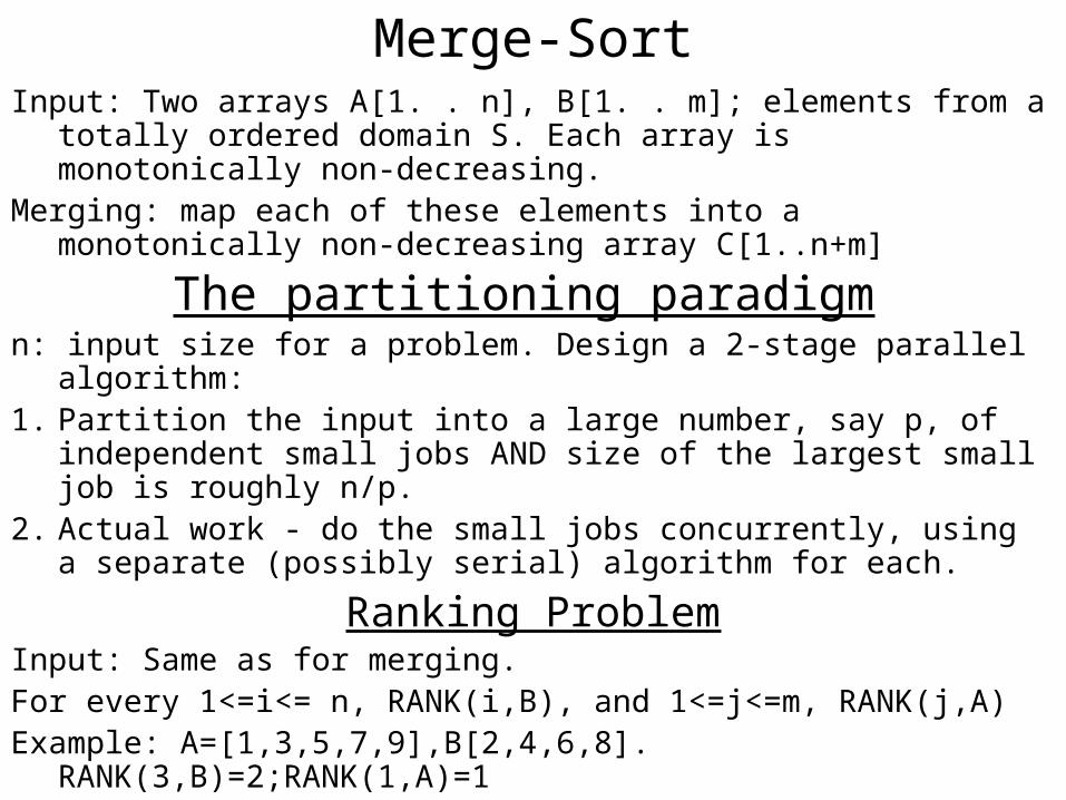
Merge-SortInput: Two arrays A[1. . n], B[1. . m]; elements from a totally

ordered domain S. Each array is monotonically non-decreasing.

Merging: map each of these elements into a monotonically non-decreasing array C[1..n+m]

The partitioning paradigm

n: input size for a problem. Design a 2-stage parallel algorithm:1. Partition the input into a large number, say p, of independent

small jobs AND size of the largest small job is roughly n/p.2. Actual work - do the small jobs concurrently, using a separate

(possibly serial) algorithm for each.

Ranking ProblemInput: Same as for merging.For every 1<=i<= n, RANK(i,B), and 1<=j<=m, RANK(j,A) Example: A=[1,3,5,7,9],B[2,4,6,8]. RANK(3,B)=2;RANK(1,A)=1

Merging algorithm (cnt’d) Observe Merging & Ranking: really same problem.Show MR in W=O(n),T=O(1) (say n=m): C(k)=A(i) RANK(i,B)=k-i-1Show RM in W=O(n),T=O(1):RANK(i,B)=jC(i+j+1)=A(i)

“Surplus-log” parallel algorithm for the Ranking for 1 ≤ i ≤ n pardo• Compute RANK(i,B) using standard binary search • Compute RANK(i,A) using binary searchComplexity: W=(O(n log n), T=O(log n)

Serial (ranking) algorithmSERIAL − RANK(A[1 . . ];B[1. .])i := 0 and j := 0; add two auxiliary elements A(n+1) and

B(n+1), each larger than both A(n) and B(n)while i ≤ n or j ≤ n do• if A(i + 1) < B(j + 1)• then RANK(i+1,B) := j; i := i + 1• else RANK(j+1),A) := i; j := j + 1In words Starting from A(1) and B(1), in each round:1. compare an element from A with an element of B2. determine the rank of the smaller among themComplexity: O(n) time (and O(n) work...)

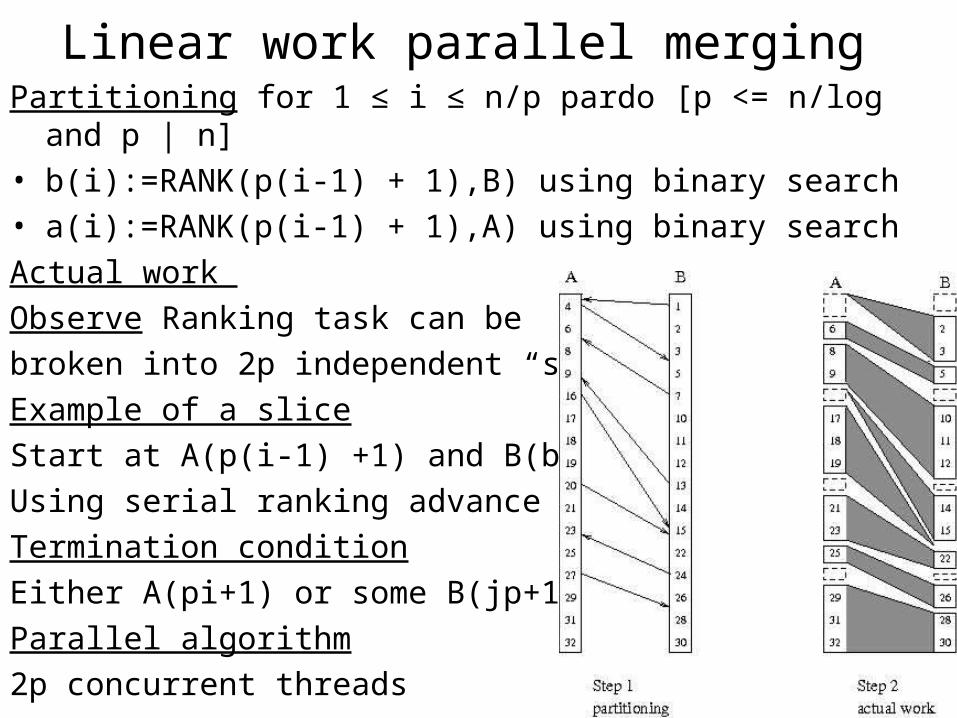
Linear work parallel mergingPartitioning for 1 ≤ i ≤ n/p pardo [p <= n/log and p | n]• b(i):=RANK(p(i-1) + 1),B) using binary search • a(i):=RANK(p(i-1) + 1),A) using binary search

Actual work

Observe Ranking task can be

broken into 2p independent “slices”.

Example of a slice

Start at A(p(i-1) +1) and B(b(i)).

Using serial ranking advance till:

Termination condition

Either A(pi+1) or some B(jp+1) loses

Parallel algorithm

2p concurrent threads

Linear work parallel merging (cont’d)

Observation 2p slices. None larger than 2n/p.

(not too bad since average is 2n/2p=n/p)

Complexity Partitioning takes O(p log n) work and O(log n) time, or O(n) work and O(log n) time. Actual work employs 2p serial algorithms, each takes O(n/p) time. Total work is O(n) and time is O(log n), for p=n/log n.

Exercise 6: Consider the merging problem as above. Consider a variant of the abovemerging algorithm where instead of fixing x (p above) to be n/ log n, x could be any positive integer between 1 and n. Describe the resulting merging algorithm and analyze its time and work complexity as a function of both x and n.

Exercise 7: Consider the merging problem as above, and assume that the values of theinput elements are not pair wise distinct. Adapt the merging algorithm for this problem,so that it will take the same work and the same running time.

Exercise 8: Consider the merging problem as above, and assume that the values of nand m are not equal. Adapt the merging algorithm for this problem. What are the newwork and time complexities?

Exercise 9: Consider the merging algorithm as above. Suppose that the algorithmneeds to be programmed using the smallest number of Spawn commands in an XMT-Csingle-program multiple-data (SPMD) program. What is the smallest number of Spawncommands possible? Justify your answer.(Note: This exercise should be given only after XMT-C programming has been intro-duced.)

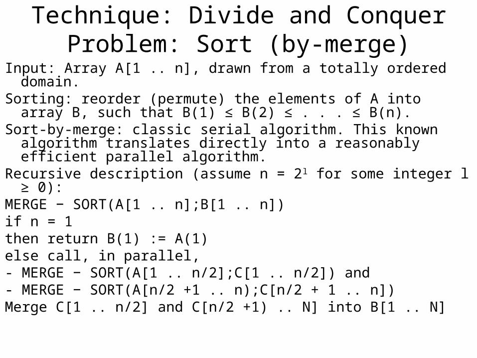
Technique: Divide and Conquer Problem: Sort (by-merge)

Input: Array A[1 .. n], drawn from a totally ordered domain.Sorting: reorder (permute) the elements of A into array B, such

that B(1) ≤ B(2) ≤ . . . ≤ B(n).Sort-by-merge: classic serial algorithm. This known algorithm

translates directly into a reasonably efficient parallel algorithm. Recursive description (assume n = 2l for some integer l ≥ 0):MERGE − SORT(A[1 .. n];B[1 .. n])if n = 1then return B(1) := A(1)else call, in parallel, - MERGE − SORT(A[1 .. n/2];C[1 .. n/2]) and- MERGE − SORT(A[n/2 +1 .. n);C[n/2 + 1 .. n])Merge C[1 .. n/2] and C[n/2 +1) .. N] into B[1 .. N]

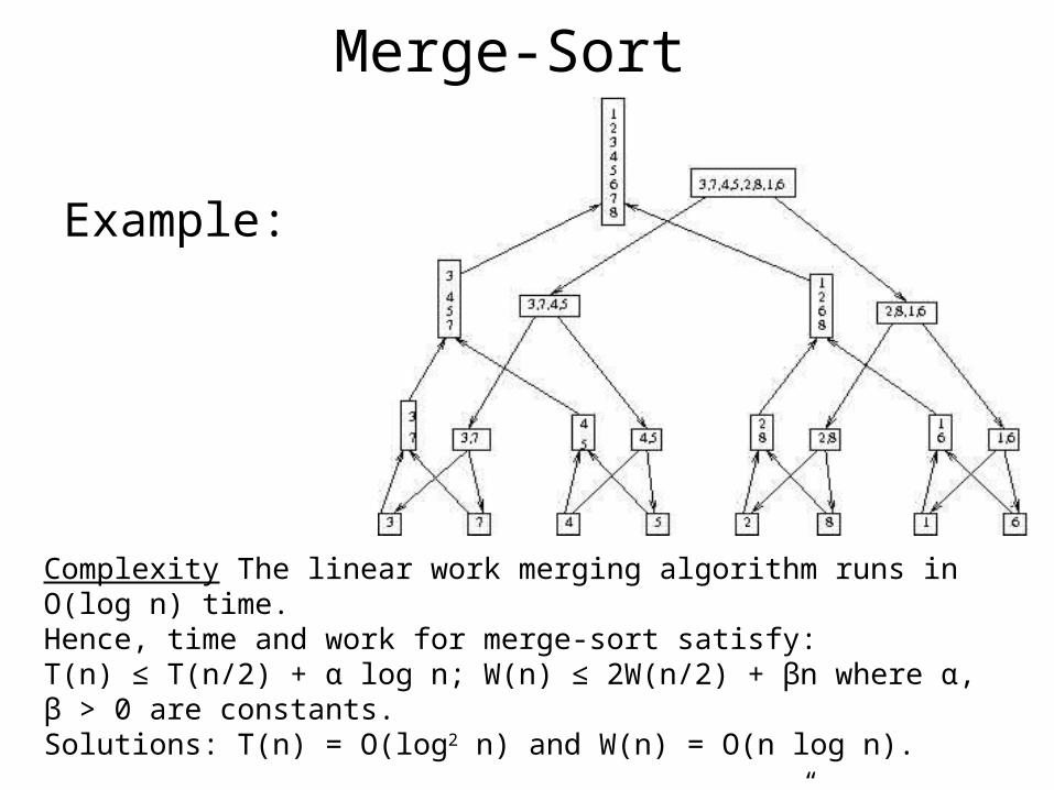
Merge-Sort

Example:

Complexity The linear work merging algorithm runs in O(log n) time. Hence, time and work for merge-sort satisfy: T(n) ≤ T(n/2) + α log n; W(n) ≤ 2W(n/2) + βn where α, β > 0 are constants. Solutions: T(n) = O(log2 n) and W(n) = O(n log n).

Merge-sort algorithm is a “balanced binary tree” algorithm. See above figure and try to give a non-recursive description of merge-sort.

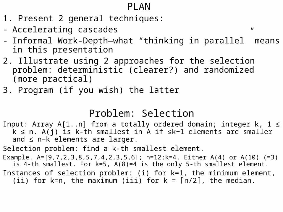
PLAN 1. Present 2 general techniques:- Accelerating cascades - Informal Work-Depth—what “thinking in parallel” means in this

presentation2. Illustrate using 2 approaches for the selection problem:

deterministic (clearer?) and randomized (more practical)3. Program (if you wish) the latter

Problem: SelectionInput: Array A[1..n] from a totally ordered domain; integer k, 1 ≤ k ≤ n. A(j) is k-

th smallest in A if ≤k−1 elements are smaller and ≤ n−k elements are larger. Selection problem: find a k-th smallest element.Example. A=[9,7,2,3,8,5,7,4,2,3,5,6]; n=12;k=4. Either A(4) or A(10) (=3) is 4-th

smallest. For k=5, A(8)=4 is the only 5-th smallest element.

Instances of selection problem: (i) for k=1, the minimum element, (ii) for k=n, the maximum (iii) for k = n/2 , the median. ⌈ ⌉

Accelerating Cascades - ExampleGet a fast O(n)-work selection algorithm from 2 “pure” selection algorithms:(1) Algorithm 1 has O(log n) iterations. Each reduces a size m instance of

selection in O(log m) time and O(m) work to an instance whose size is ≤ 3m/4. Why is the complexity of Algorithm 1 O(log2n) time and O(n) work?

(2) Algorithm 2 runs in O(log n) time and O(n log n) work.Pros: Algorithm 1: only O(n) work. Algorithm 2: less time. Accelerating cascades technique way for deriving a single algorithm that is

both: fast and needs O(n) work. Main idea start with Algorithm 1, but not run it to completion. Instead, switch to

Algorithm 2, as follows:Step 1 Use Algorithm 1 to reduce selection from n to ≤ n/ log n. Note: O(log log

n) rounds are enough, since for (3/4)rn ≤ n/ log n, we need (4/3)r ≥ log n, implying r = log4/3log n.

Step 2 Apply Algorithm 2.Complexity Step 1 takes O(log n log log n) time. The number of operations is

n+(3/4)n+.. which is O(n). Step 2 takes additional O(log n) time and O(n) work. In total: O(log n log log n) time, and O(n) work.

Accelerating cascades is a practical technique.

Algorithm 2 is actually a sorting algorithm.

Accelerating Cascades

Consider the following situation: for problem of size n, there are two parallel algorithms.

Algorithm A: W1(n) and T1(n). Algorithm B: W2(n) and T2(n) time. Suppose: Algorithm A is more efficient (W1(n) < W2(n)), while Algorithm B is faster (T1(n) < T2(n) ). Assume also: Algorithm A is a “reducing algorithm”: Given a problem of size n, Algorithm A operates in phases. Output of each successive phase is a smaller instance of the problem. The accelerating cascades technique composes a new algorithm as follows:

Start by applying Algorithm A. Once the output size of a phase of this algorithm is below some threshold, finish by switching to Algorithm B.

Algorithm 1, and IWD ExampleNote: not just a selection algorithm. Interest is broader, as the

informal work-depth (IWD) presentation technique is illustrated. In line with the IWD presentation technique, some missing details for the current high-level description of Algorithm 1 are filled in later.

Input Array A[1..n]; integer k, 1 ≤ k ≤ n. Algorithm 1 works in “reducing” ITERATIONS:Input: Array B[1..m]; 1≤ k0≤m. Find k0-th element in B. Main idea behind a reducing iteration is: find an element α of B

which is guaranteed to be not too small (≤ m/4 elements of B are smaller), and not too large (≤ m/4 elements of B are larger). Exact ranking of α in B enables to conclude that at least m/4 elements of B do not contain the k0-th smallest element. Therefore, they can be discarded. The other alternative: the k0-th smallest element (which is also the k-th smallest element with respect to the original input) has been found.

ALGORITHM 1 - High-level description (Assume: log m and m/ log m are integers.)1. for i, 1 ≤ i ≤ n pardo B(i) := A(i)2. k0 := k; m := n3. while m > 1 do3.1. Partition B into m/log m blocks, each of size log m as follows. Denote the blocks B1,..,Bm/log m, where B1=B[1..logm],..,Bm/log m=B[m+1−log m..m].3.2. for block Bi, 1 ≤ i ≤ m/log m pardo compute the median αi of Bi, using a linear time serial selection algorithm3.3. Apply a sorting algorithm to find α the median of medians (α1, . . . , αm/log m).3.4. Compute s1, s2 and s3. s1: # elements in B smaller than α, s2: # elements equal to α, and s3: # elements larger than α.3.5. There are three possibilities:3.5.1 (i) k0≤s1: the new subset B (the input for the next iteration) consists of the elements in B, which are smaller than α (m:=s1; k0 remains the same)3.5.2 (ii) s1<k0≤s1+s2: α is the k0-th smallest element in B; algorithm terminates3.5.3 (iii) k0>s1+s2: the new subset B consists of the elements in B, which are larger than α (m := s3; k0:=k0−(s1+s2) )4. (we can reach this instruction only with m = 1 and k0 = 1) B(1) is the k0-th element in B.

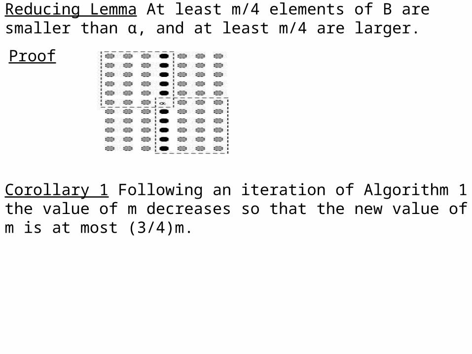
Reducing Lemma At least m/4 elements of B are smaller than α, and at least m/4 are larger.

Proof

Corollary 1 Following an iteration of Algorithm 1 the value of m decreases so that the new value of m is at most (3/4)m.

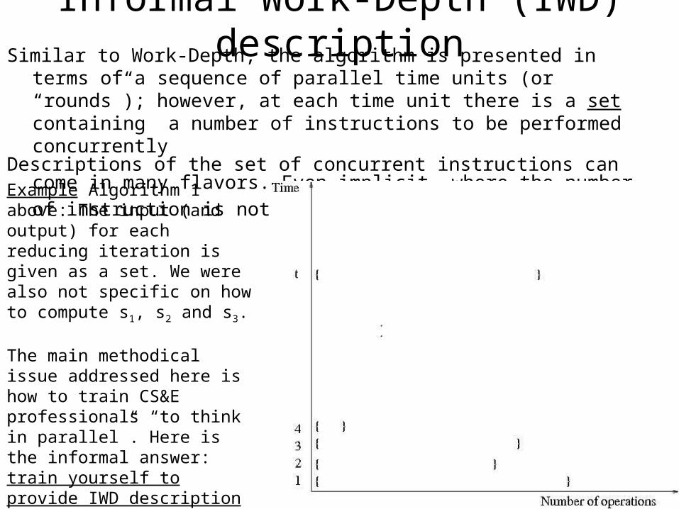
Informal Work-Depth (IWD) descriptionSimilar to Work-Depth, the algorithm is presented in terms of a sequence of

parallel time units (or “rounds”); however, at each time unit there is a set containing a number of instructions to be performed concurrently

Descriptions of the set of concurrent instructions can come in many flavors.

Even implicit, where the number of instruction is not obvious.

Example Algorithm 1 above: The input (and output) for each reducing iteration is given as a set. We were also not specific on how to compute s1, s2 and s3.

The main methodical issue addressed here is how to train CS&E professionals “to think in parallel”. Here is the informal answer: train yourself to provide IWD description of parallel algorithms. The rest is detail (although important) that can be acquired as a skill (also a matter of training).

The Selection Algorithm (wrap-up)To derive the lower level description of Algorithm 1, simply apply

the prefix-sums algorithm several times. Theorem 5.1 Algorithm 1 solves the selection problem in O(log2n)

time and O(n) work. The main selection algorithm, composed of algorithms 1 and 2, runs in O(n) work and O(log n log log n) time.

Exercise 10 Consider the following sorting algorithm. Find the median element and then continue by sorting separately the elements larger than the median and the ones smaller than the median. Explain why this is indeed a sorting algorithm. What will be the time and work complexities of such algorithm?

Recap: (i) Accelerating cascades framework was presented and illustrated by selection algorithm. (ii) A top-down methodology for describing parallel algorithms was presented. Its upper level, called Informal Work-Depth (IWD), is proposed as the essence of thinking in parallel.

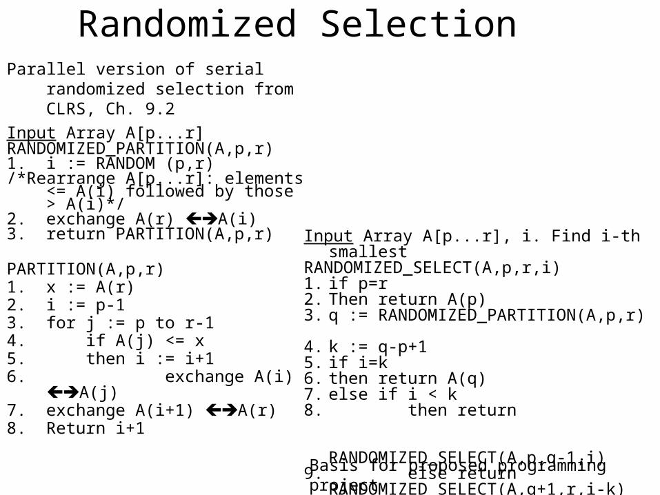
Randomized SelectionParallel version of serial randomized

selection from CLRS, Ch. 9.2

Input Array A[p...r]RANDOMIZED_PARTITION(A,p,r) 1. i := RANDOM (p,r)/*Rearrange A[p...r]: elements <=

A(i) followed by those > A(i)*/2. exchange A(r) A(i)3. return PARTITION(A,p,r)

PARTITION(A,p,r)1. x := A(r)2. i := p-13. for j := p to r-14. if A(j) <= x5. then i := i+16. exchange A(i) A(j) 7. exchange A(i+1) A(r)8. Return i+1

Input Array A[p...r], i. Find i-th smallestRANDOMIZED_SELECT(A,p,r,i)1. if p=r2. Then return A(p)3. q := RANDOMIZED_PARTITION(A,p,r) 4. k := q-p+15. if i=k6. then return A(q) 7. else if i < k8. then return

RANDOMIZED_SELECT(A,p,q-1,i)

9. else return RANDOMIZED_SELECT(A,q+1,r,i-k)

Basis for proposed programming project

Integer SortingInput Array A[1..n], integers from range [0..r−1]; n and r are

positive integers.Sorting: rank from smallest to largest.Assume n is divisible by r. Typical value for r might be n1/2; other

values possible.Two comments about the parallel integer sorting algorithm:(i) Its performance depends on the value of r, and unlike other

parallel algorithms we have seen, its running time may not be bounded by O(logkn) for any constant k (“poly-logarithmic”). It is a remarkable coincidence that the literature includes only very few work-efficient non ploy-log parallel algorithms.

(ii) It already lent itself to efficient implementation on a few parallel machines in the early 1990s. (Remark later.)

The algorithm work as follows:

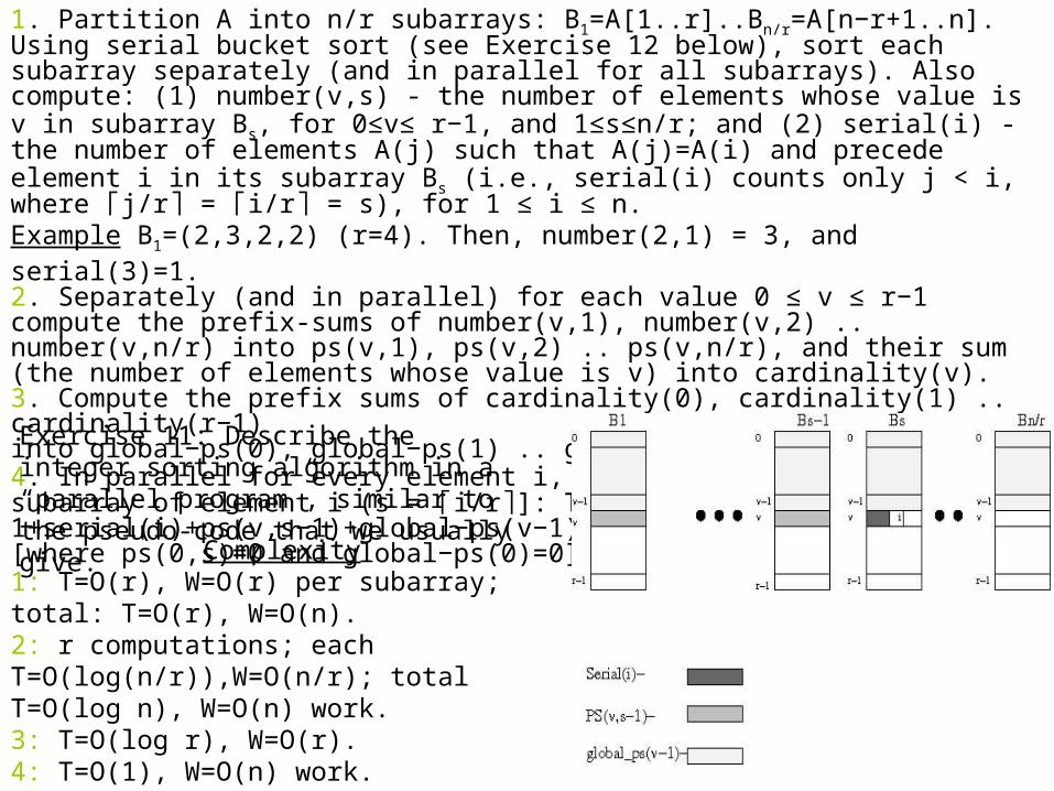
1. Partition A into n/r subarrays: B1=A[1..r]..Bn/r=A[n−r+1..n]. Using serial bucket sort (see Exercise 12 below), sort each subarray separately (and in parallel for all subarrays). Also compute: (1) number(v,s) - the number of elements whose value is v in subarray Bs, for 0≤v≤ r−1, and 1≤s≤n/r; and (2) serial(i) - the number of elements A(j) such that A(j)=A(i) and precede element i in its subarray Bs (i.e., serial(i) counts only j < i, where j/r = i/r ⌈ ⌉ ⌈ ⌉= s), for 1 ≤ i ≤ n.Example B1=(2,3,2,2) (r=4). Then, number(2,1) = 3, and serial(3)=1.2. Separately (and in parallel) for each value 0 ≤ v ≤ r−1 compute the prefix-sums of number(v,1), number(v,2) .. number(v,n/r) into ps(v,1), ps(v,2) .. ps(v,n/r), and their sum (the number of elements whose value is v) into cardinality(v).3. Compute the prefix sums of cardinality(0), cardinality(1) .. cardinality(r−1)into global−ps(0), global−ps(1) .. global−ps(r−1).4. In parallel for every element i, 1≤i≤n [Let v = A(i) and Bs the subarray of element i (s = i/r ]: The rank of element i is 1+serial(i)+ps(v,s−1)+global−ps(v−1)⌈ ⌉

[where ps(0,s)=0 and global−ps(0)=0]

Exercise 11: Describe the integer sorting algorithm in a “parallel program”, similar tothe pseudo-code that we usually give.

Complexity 1: T=O(r), W=O(r) per subarray; total: T=O(r), W=O(n). 2: r computations; each T=O(log(n/r)),W=O(n/r); total T=O(log n), W=O(n) work. 3: T=O(log r), W=O(r). 4: T=O(1), W=O(n) work. Total: T=O(r + log n), W=O(n).

Theorem 6.1: (1) The integer sorting algorithm runs in O(r+log n) time and O(n) work. (2) The integer sorting algorithm can be applied to run in time O(k(r1/k+log n)) and O(kn) work for any positive integer k.Showed (1). For (2): radix sort using the basic integer sort (BIS) algorithm:A sorting algorithm is stable if for every pair of two equal input elements A(i) = A(j) where 1 ≤ i < j ≤ n, it ranks element i lower than element j. Observe: BIS is stable. Only outline the case k = 2.

2-step algorithm for an integer sort problem with r=n in T=O(√n) W=O(n)Note: the big Oh notation suppresses the factor k=2. Assume that √n is an integer.Step 1 Apply BIS to keys A(1) (mod √n), A(2) (mod √n) .. A(n) (mod √n). If the computed rank of an element i is j then set B(j) := A(i).Step 2 Apply again BIS this time to key B(1)/√n , B(2)/√n .. B(n)/√n .⌊ ⌋ ⌊ ⌋ ⌊ ⌋

Example 1. Suppose UMD has 35,000 students with social security number as IDs. Sort by IDs. The value of k will be 4 since √1B ≤ 35,000 and 4 steps are used.2. Let A=10,12,9,2,3,11,10,12,4,5,9,4,3,7,15,1 with n=16 and r=16. Keys for Step 1 are values modulo 4: 2,0,1,2,3,3,2,0,0,1,1,0,3,3,3,1. Sorting & assignment to array B: 12,12,4,4,9,5,9,1,10,2,10,3,11,3,15. Keys for Step 2 are v/4 , where v is the value of an ⌊ ⌋element of B (i.e., 9/4 =2). The keys are 3,3,1,1,2,1,2,0,2,0,2,0,2,0,3. The result relative ⌊ ⌋to the original values of A is 1,2,3,3,4,5,7,9,9,10,10,11,12,12,15.

Remarks 1. This simple integer sorting algorithm has led to efficient implementationon parallel machines such as some Cray machines and the Connection Machine (CM-2). [BLM+91] and [ZB91] report giving competitive performance on the machines that they examined. Given a parallel computer architecture where the local memories of different (physical) processors are distant from one another, the algorithm enables partitioning of the input into these local memories without any inter-processorcommunication. In steps 2 and 3, communication is used for applying the prefix-sumsroutine. Over the years, several machines had special constructs that enable very fastimplementation of such a routine.2. Since the theory community looked favorably at the time only on poly-log time algorithm, this practical sorting algorithm was originally presented in [CV-86] for a routine for sorting integers in the range 1 to log n as was needed for another algorithm.

Exercise 12: (Redundant if you remember the serial bucket-sort algorithm).The serial bucket-sort (called also bin-sort) algorithm works as follows. Input: An arrayA = A(1), . . . ,A(n) of integers from the range [0, . . . , n−1]. For each value v, 0 ≤ v ≤ n−1, the algorithm forms a linked list of all elements A(i) = v, 0 ≤ i ≤ n−1. Initially,all lists are empty. Then, at step i, 0 ≤ i ≤ n − 1, element A(i) is inserted to the linkedlist of value v, where v = A(i). Finally, the linked list are traversed from value 0 tovalue n − 1, and all the input elements are ranked. (1) Describe this serial bucket-sortalgorithm in pseudo-code using a “structured programming style”. Make sure that theversion you describe provides stable sorting. (2) Show that the time complexity is O(n).

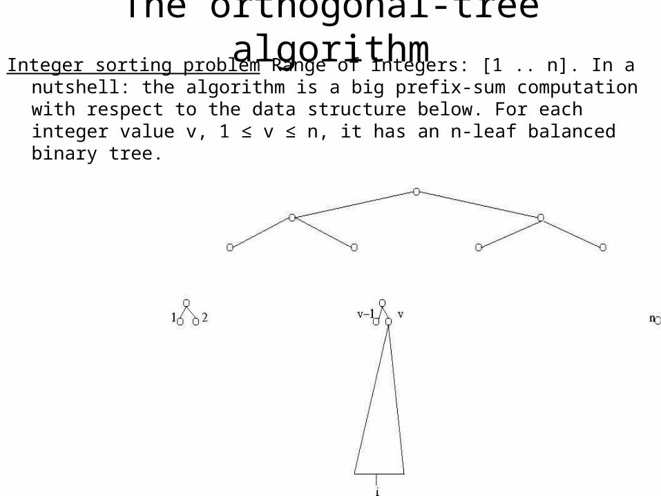
The orthogonal-tree algorithmInteger sorting problem Range of integers: [1 .. n]. In a nutshell: the algorithm is

a big prefix-sum computation with respect to the data structure below. For each integer value v, 1 ≤ v ≤ n, it has an n-leaf balanced binary tree.

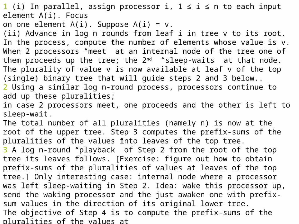
1 (i) In parallel, assign processor i, 1 ≤ i ≤ n to each input element A(i). Focuson one element A(i). Suppose A(i) = v. (ii) Advance in log n rounds from leaf i in tree v to its root. In the process, compute the number of elements whose value is v. When 2 processors “meet” at an internal node of the tree one of them proceeds up the tree; the 2nd “sleep-waits” at that node.The plurality of value v is now available at leaf v of the top (single) binary tree that will guide steps 2 and 3 below..2 Using a similar log n-round process, processors continue to add up these pluralities;in case 2 processors meet, one proceeds and the other is left to sleep-wait. The total number of all pluralities (namely n) is now at the root of the upper tree. Step 3 computes the prefix-sums of the pluralities of the values into leaves of the top tree.3 A log n-round “playback” of Step 2 from the root of the top tree its leaves follows. [Exercise: figure out how to obtain prefix-sums of the pluralities of values at leaves of the top tree.] Only interesting case: internal node where a processor was left sleep-waiting in Step 2. Idea: wake this processor up, send the waking processor and the just awaken one with prefix-sum values in the direction of its original lower tree.The objective of Step 4 is to compute the prefix-sums of the pluralities of the values atevery leaf of the lower trees that holds an input element-- the leaves active in Step 1(i). 4 A log n-round “playback” of Step 1, starting in parallel at the roots of the lower trees. Each of the processors ends at the original leaf in which it started Step 1. [Exercise: Same as Step 3]. Waking processors and computing prefix-sums: Step 3.

Exercise 13: (i) Show how to complete the above description into a sorting algorithmthat runs in T=O(log n), W=O(n log n) and O(n2) space. (ii) Explain why youralgorithm indeed achieves this complexity result.

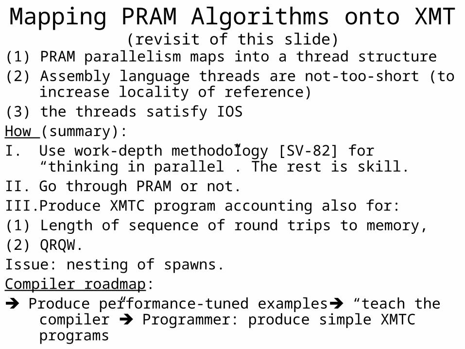
Mapping PRAM Algorithms onto XMT(revisit of this slide)

(1) PRAM parallelism maps into a thread structure(2) Assembly language threads are not-too-short (to increase

locality of reference)(3) the threads satisfy IOSHow (summary):I. Use work-depth methodology [SV-82] for “thinking in

parallel”. The rest is skill. II. Go through PRAM or not.III. Produce XMTC program accounting also for: (1) Length of sequence of round trips to memory,(2) QRQW. Issue: nesting of spawns.Compiler roadmap: Produce performance-tuned examples “teach the compiler”

Programmer: produce simple XMTC programs

Back-up slides

But coming up with a whole theory of parallel algorithms is a complex mental problem

How to address that?1. Address first the easiest problem(s) you

don’t know to solve.Provided a surprising structure, as illustrated next.

2. Do what computer scientists do best: develop/identify/fit the correct level of abstraction to each problemHas been a key point of this presentation

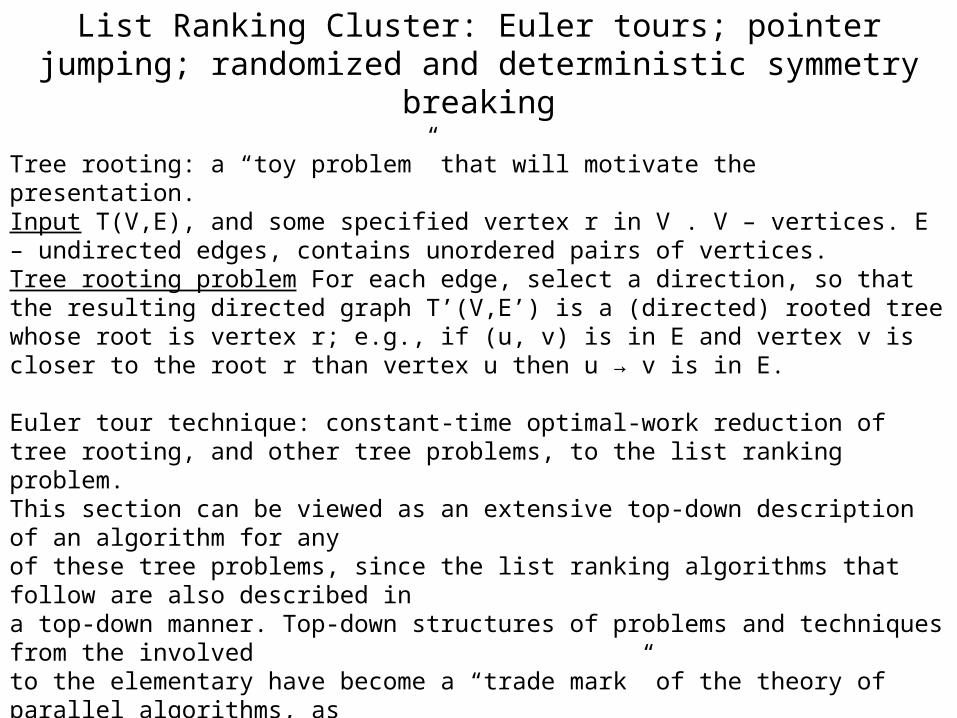
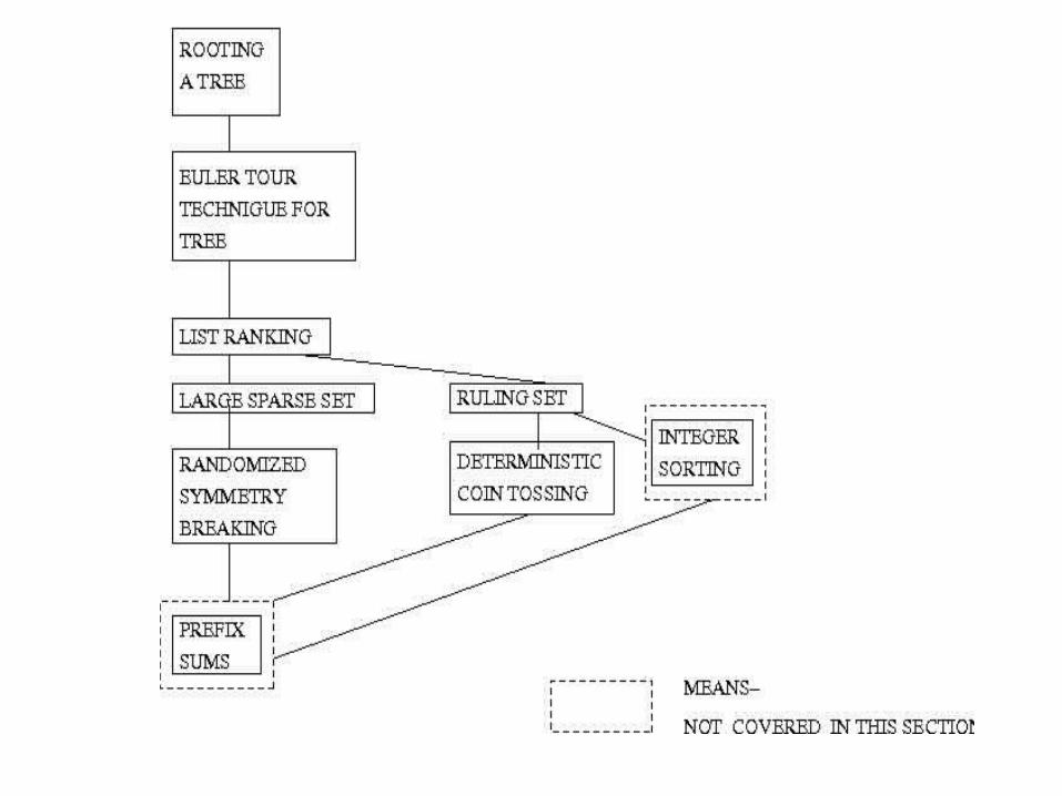
List Ranking Cluster: Euler tours; pointer jumping; randomized and deterministic symmetry breaking

Tree rooting: a “toy problem” that will motivate the presentation. Input T(V,E), and some specified vertex r in V . V – vertices. E – undirected edges, contains unordered pairs of vertices. Tree rooting problem For each edge, select a direction, so that the resulting directed graph T’(V,E’) is a (directed) rooted tree whose root is vertex r; e.g., if (u, v) is in E and vertex v is closer to the root r than vertex u then u → v is in E.

Euler tour technique: constant-time optimal-work reduction of tree rooting, and other tree problems, to the list ranking problem.This section can be viewed as an extensive top-down description of an algorithm for anyof these tree problems, since the list ranking algorithms that follow are also described ina top-down manner. Top-down structures of problems and techniques from the involvedto the elementary have become a “trade mark” of the theory of parallel algorithms, asreviewed in [Vis91]. Such fine structures highlight the elegance of this theory and aremodest, yet noteworthy, of fine structures that exist in some classical fields of Mathe-matics. However, they are rather unique for Combinatorics-related theories. Figure toillustrate this structure:

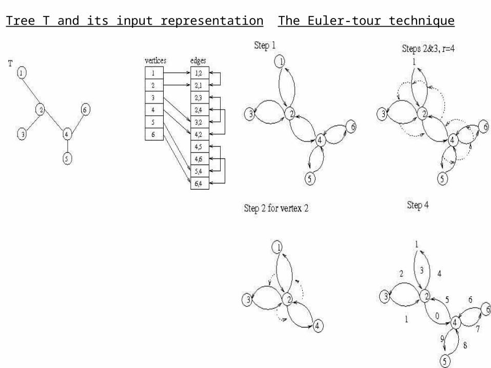
Tree T and its input representation The Euler-tour technique