encyclopedia of earthquake engineering || time history seismic analysis

Time History Seismic Analysis

Nikos D. Lagaros*, Chara Ch. Mitropoulou and Manolis PapadrakakisInstitute of Structural Analysis & Antiseismic Research, Department of Structural Engineering, School of CivilEngineering, National Technical University of Athens, Athens, Greece

Synonyms

Artificial accelerograms; Direct integration methods; Inertia and damping forces; Linear andnonlinear analysis; Natural records; Seismic loading

Introduction

Most of the current seismic design codes belong to the category of prescriptive design procedures(or limit-state design procedures), where if a number of checks are satisfied, then the structure isconsidered safe since it fulfills the safety criterion against collapse. A typical limit-state-baseddesign can be viewed as one- (i.e., ultimate strength) or two-limit-state approach (i.e., serviceabilityand ultimate strength). Existing seismic design procedures are based on the principle that a structurewill avoid collapse if it is designed to absorb and dissipate the kinetic energy that is induced duringa seismic excitation. Most of the modern seismic norms express the ability of the structure to absorbenergy through inelastic deformation using a reduction or behavior factor that depends on thematerial and the construction type of the structure. The concept of performance-based design(PBD) was introduced a few decades ago, for designing structures subjected to seismic loadingconditions. In PBD more accurate and time-consuming analysis procedures are employed, toestimate nonlinear structural response. The progress that takes place in the area of computationalmechanics, as well as in computer technology, continuously expands the capabilities and theapplicability of PBD procedures. The main objective of this kind of design procedures is to achievemore predictable and reliable levels of safety and operability against natural hazards. According toPBD procedures, the structures should be able to resist earthquakes in a quantifiable manner and topresent specific target performance levels of possible damages. PBD criteria try to define certainlevels of structural performance for various levels of seismic hazard.

In the construction industry, decision making for structural systems situated in seismically activeregions requires consideration of damage cost and other losses resulting from earthquakes occurringduring the life span of a structure. Thus, nowadays, life-cycle cost analysis (LCCA) becomes anessential component of the design process used to control the initial and the future cost of buildingownership. In the early 1960s, LCCA was applied in the commercial area and in particular in thedesign of products considering the total cost of developing, producing, using, and retiring. Theintroduction of LCCA in the construction industry was made in the field of infrastructures as aninvestment assessment tool. In particular, in the early 1980s, it was used in the USA as an appraisaltool for the total cost of ownership over the life span of an asset. Later, in view of large losses due toextreme hazards, like earthquakes and hurricanes, there was a need for new design procedures offacilities that could lead to life protection and reduction of damage and economical impact of such

*Email: [email protected]

Encyclopedia of Earthquake EngineeringDOI 10.1007/978-3-642-36197-5_134-1# Springer-Verlag Berlin Heidelberg 2013

of 19

http://link.springer.com/SpringerLink:ChapterTarget







hazards to an acceptable level. In this context LCCAwas introduced in the field of constructions asa complex investment appraisal tool incorporating a structural performance criterion.

Over the last decades, risk management of structural systems has gained the attention of variouseconomic and technical decision centers in modern society. The optimal allocation of the publicresources for a sustainable economy requires proper tools for estimating the consequences of naturalhazardous events on the built environment. The risk management addresses this claim indicating theway for implementing optimal choices. Thus, the main purpose of the risk management process is tochoose among different options relying on technical and economical considerations. Risk assess-ment and decision analysis are the main steps of the risk management concept. It is thereforeessential to establish a reliable procedure for assessing the seismic risk of structural systems. Seismicfragility analysis, which provides a measure of the safety margin for the structural system, isconsidered as the core of the risk assessment framework.

The implementation of PBD, LCCA, or seismic risk procedures requires a reliable computing toolfor estimating the capacity and the demand for any structural system. Some of these computing tools(Fajfar 2000; Chopra and Goel 2002; Vamvatsikos and Cornell 2002) are based on time historyseismic analyses, and they are considered as analysis methods for obtaining good estimates of thestructural performance in the case of earthquake hazard, and therefore, they are considered asappropriate methods to be incorporated into such design and assessment frameworks. In thisentry, we provide an overview of the time history seismic analysis applied for design and assessmentpurposes.

Ground Motion Excitation

Selecting the seismic loading for design and/or assessment purposes is not an easy task due to theuncertainties involved in the very nature of seismic excitations. One possible approach for thetreatment of the seismic loading is to assume that the structure is subjected to a set of records that aremore likely to occur in the region where the structure is located.

Natural RecordsFor the implementation of dynamic seismic analysis, a scale factor is calculated for each hazard levelconsidered and for each one of the records selected. In order to preserve the relative scale of the twocomponents of the records in the longitudinal and transversal directions, the component of the recordhaving the highest SA(T1,5 %) is scaled first, while the scaling factor that preserves their relative ratiois assigned to the second component.

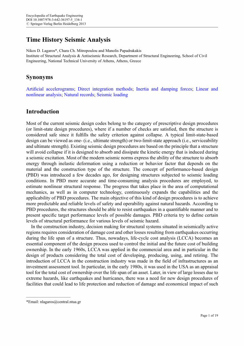
Generation of Artificial AccelerogramsIn order for the artificial accelerograms to be representative, they have to match some requirementsof the seismic codes. The most essential one is that the accelerograms have to be compatible with theelastic design response spectrum of the region. Each accelerogram corresponds to a single responsespectrum for a given damping ratio. On the other hand, on each response spectrum corresponds aninfinite number of accelerograms. Gasparini and Vanmarke (1976) were the first to propose thecreation of artificial accelerograms based on a specific response spectrum. The mean (m) responsespectrum is depicted in Fig. 1, along with its dispersion (m + s and m� s denoted with dotted lines)for the case of the natural class of records (NAT) selected by PEER (2012) and artificialaccelerograms (ART) generated according to the procedure described below in this section. Theresponse spectra for the NAT class of records were obtained after scaling the records to the same


of 19

SA(T1,5%), where T1¼ 0.628 s for the 40/50 hazard level, in accordance with the hazard curve of thecity of San Diego, California. Comparing NAT and ART class of accelerograms, it can be seen thatthe dispersion of the response spectra for the ART class of accelerograms is lower than that of theNAT class.

Intensity MeasuresEarthquake engineering is a scientific field strongly connected with the effect of strong groundmotions on people and environment. Strong ground motions are extremely complicated and a lot ofdata is required for their full description. The definition of a number of ground motion parameters,namely, intensity measures (IMs), simplifies the description of a strong ground motion and links theseismic hazard with the structural data required for the solution of earthquake engineering problems.The most significant characteristics of a ground motion from an earthquake engineering point ofview are the frequency content, the amplitude, and the motion duration. Some of the IMs are relatedto amplitude or to frequency content, to duration, or to more than one of the three essential groundmotion characteristics. The IMs that are related to the effect of more than one ground motioncharacteristics are considered more reliable for the description of a ground motion and are mostsuitable to reflect the potential damage that a ground motion can produce.

The most commonly used amplitude IMs derived from an accelerogram are the peak groundacceleration (high-frequency component), peak velocity (intermediate-frequency component), peakdisplacement (low-frequency component), sustained maximum acceleration and velocity, and theeffective design acceleration. Amplitude IMs are used for the derivation of empirical attenuationrelationships used in probabilistic hazard analysis, because their production is based on IMs’dependence, on the magnitude of the earthquake, and on the site-to-source distance. Frequencycontent IMs describe through different types of spectra how the amplitude of a ground motion isdistributed among different frequencies. IMs related to frequency content are Fourier spectra andpower spectra that correspond to the frequency content of the ground motion itself and the responsespectra that correspond to the influence of the ground motion on structures with different firsteigenperiods. Among these types of IMs are spectral parameters, like the predominant period,bandwidth, central frequency, shape factor, Kanai-Tajimi parameters, and the ratio vmax/amax

which describes the frequency content of a ground motion. The most commonly used durationIM is the bracketed duration which is defined as the time between the first and the last exceedance ofa threshold acceleration, usually equal to 0.05 g.

Arias intensity (IA), characteristic intensity (IC), and cumulative absolute velocity (CAV) are threeIMs that reflect the amplitude, the frequency content, and the duration of a strong ground motion,

0 0.5 1 1.5 2 2.5 3 3.5 40

1

2

3

4

5

6

7

8a b

T (sec)

SA(T

1,5%

) (m

/sec

2 )

SA(T

1,5%

) (m

/sec

2 )

0 0.5 1 1.5 2 2.5 3 3.5 40

2

4

6

8

10

12

14

T (sec)

Fig. 1 Mean response spectra of the records for the class of (a) artificial accelerograms and (b) natural records (dottedlines represent the m + s and m � s response spectra)


of 19

respectively, which correlate well with structural damage. Arias intensity is defined as the timeintegral of the square of the ground acceleration

IA ¼ p2g

ð1

0

a tð Þ½ �2dt (1)

where a(t) is the ground acceleration and g is the acceleration due to gravity (9.81 m/s) and isexpressed in units of velocity, i.e., meter per second. The symbol of infinity in the time integrationmeans that IA is calculated over the entire duration and not over the duration of the strong groundmotion Td that is defined through specific methods.

Characteristic intensity is defined as

IC ¼ a1:5rmsT0:5d (2)

where arms is the rms acceleration (root mean square acceleration) ground motion parameter and Tdis the duration of the strong motion.

Cumulative absolute velocity is defined as the integral of the absolute acceleration in a timehistory, and it is obtained through the following equation:

CAV ¼ðTd

0

a tð Þj jdt (3)

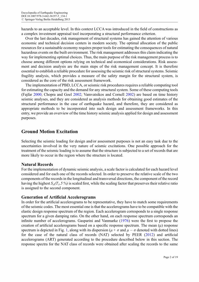
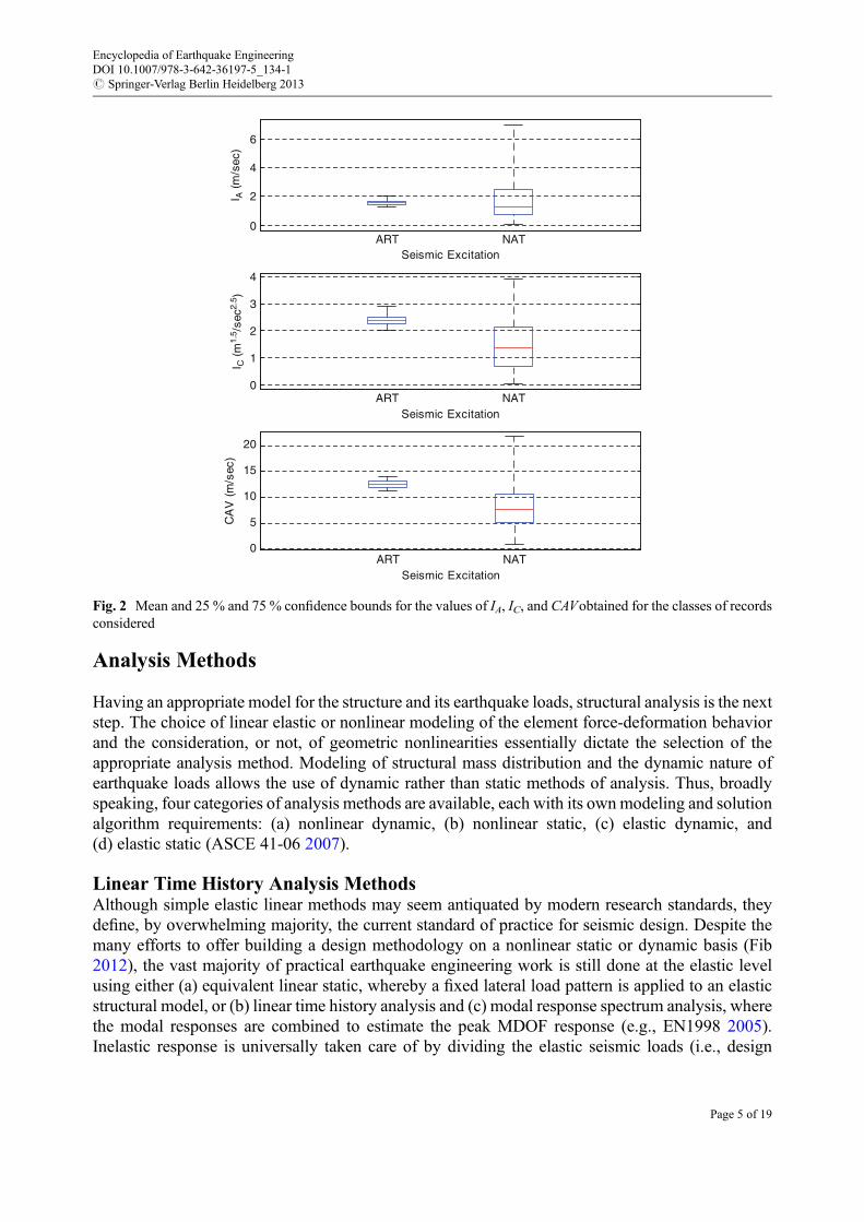
where |a(t)| is the absolute value of the acceleration time series at time t and Td is the duration of thestrong motion. CAVexpresses the absolute area under the absolute accelerogram and corresponds tothe cumulative absolute velocity that is well correlated with structural damage (Kramer 1996). Thesethree IMs are used for investigating their dispersion with reference to the two classes of seismicexcitations considered. In particular, the characteristic intensity is a measure that is related to anindex that quantifies the damage due to the maximum deformation and the absorbed hystereticenergy. In order to examine the influence of the class of seismic excitations considered on the valuesof the three IMs, the box plots depicted in Fig. 2 have been generated for the 40/50 hazard level(denoting 40 % probability of exceedance in 50 years).

For each IM considered and for each class of seismic excitation, a box plot was created. On eachbox, the central mark denoted with a bold black line is the median value of the IM in question. Theedges of the box represent the 25 % and 75 % percentiles, while the whiskers denoted with blacklines extend to the most extreme data points, i.e., represent the range of the IM values. For all threeIMs, ARTclass of accelerograms has the narrower range and confidence bounds. On the other hand,the median values of ART are close to each other while NAT varies significantly for the case of ICand CAV. For the case of IA, the three median values are quite close. For the 25 % and 75 %percentiles, IC and CAV, NAT class of seismic excitations, have similar box sizes denoting that theyare related to the length of the range of values.


of 19

Analysis Methods

Having an appropriate model for the structure and its earthquake loads, structural analysis is the nextstep. The choice of linear elastic or nonlinear modeling of the element force-deformation behaviorand the consideration, or not, of geometric nonlinearities essentially dictate the selection of theappropriate analysis method. Modeling of structural mass distribution and the dynamic nature ofearthquake loads allows the use of dynamic rather than static methods of analysis. Thus, broadlyspeaking, four categories of analysis methods are available, each with its ownmodeling and solutionalgorithm requirements: (a) nonlinear dynamic, (b) nonlinear static, (c) elastic dynamic, and(d) elastic static (ASCE 41-06 2007).

Linear Time History Analysis MethodsAlthough simple elastic linear methods may seem antiquated by modern research standards, theydefine, by overwhelming majority, the current standard of practice for seismic design. Despite themany efforts to offer building a design methodology on a nonlinear static or dynamic basis (Fib2012), the vast majority of practical earthquake engineering work is still done at the elastic levelusing either (a) equivalent linear static, whereby a fixed lateral load pattern is applied to an elasticstructural model, or (b) linear time history analysis and (c) modal response spectrum analysis, wherethe modal responses are combined to estimate the peak MDOF response (e.g., EN1998 2005).Inelastic response is universally taken care of by dividing the elastic seismic loads (i.e., design

0

2

4

6

NATARTSeismic Excitation

I A (

m/s

ec)

0

1

2

3

4



I C (

m1.

5 /se

c2.5 )

0

5

10

15

20

CA

V (

m/s

ec)

Fig. 2 Mean and 25 % and 75 % confidence bounds for the values of IA, IC, and CAVobtained for the classes of recordsconsidered


of 19

spectral acceleration values) by the appropriate reduction R (or behavior q) factor that is meant torepresent the ductility and overstrength of a yielding system. Although little recent research has beendirected in the way of elastic methods, recent advancements in nonlinear analysis have helped toshed some light into the premise of using elastic results to capture nonlinear behavior.

The equilibrium equations for a system in motion can be written as

M€u tð Þ þ C _u tð Þ þKu tð Þ ¼ R tð Þ (4)

whereM,C, andK are the mass, damping, and stiffness matrices andR(t) is the external load vector,while u tð Þ, _u tð Þ, and €u tð Þ are the displacement, velocity, and acceleration vectors of the finiteelement assemblage, respectively. The choice for a static or dynamic analysis (i.e., for including orneglecting velocity and acceleration-dependent forces in the analysis) is usually decided by engi-neering judgment. Mathematically, Eq. 4 represents a system of linear differential equations ofsecond order and the solution of this system can be obtained by standard procedures for the solutionof differential equations. In practical finite element analysis, we are mainly interested in a feweffective methods and we will concentrate in the next sections on the presentation of thosetechniques and in particular on the direct integration ones. In direct integration the system of lineardifferential equations in Eq. 4 is integrated using a numerical step-by-step procedure; the term“direct” means that no transformation of the equations is carried out prior to the numericalintegration.

Central Difference MethodOne procedure that can be very effective in the solution of certain problems is the central differencemethod where it is assumed that

€u tð Þ ¼ 1

Dt2u t� Dtð Þ � 2u tð Þ þ u tþ Dtð Þ½ � (5)

and the velocity expansion is defined by

_u tð Þ ¼ 1

2Dtu tþ Dtð Þ � u t� Dtð Þ½ � (6)

The displacement expression for time t + Dt is obtained by substituting Eqs. 5 and 6 into Eq. 4:

1

Dt2Mþ 1

2DtC

� �u tþ Dtð Þ ¼ R tð Þ � K � 2

Dt2M

� �u tð Þ � 1

Dt2M� 1

2DtC

� �u t� Dtð Þ (7)

from which we can solve for u(t + Dt). It should be noted that the solution of u(t + Dt) is based onusing the equilibrium conditions of Eq. 4 at time t. For this reason the integration procedure is calledan explicit integration method. On the other hand, the Houbolt, Wilson, and Newmark methods,considered in the next sections, use the equilibrium conditions at time t + Dt and are called implicitintegration methods.

Houbolt MethodThe Houbolt integration scheme is somewhat related to the central difference method in the sensethat standard finite difference expressions are used to approximate the acceleration and velocity


of 19

components in terms of displacement. The following expansions are employed in the Houbolt(1950) integration method:

€u tþ Dtð Þ ¼ 1

Dt22u tþ Dtð Þ � 5u tð Þ þ 4u t� Dtð Þ � u t� 2Dtð Þ½ � (8)

and

_u tþ Dtð Þ ¼ 1

6Dt11u tþ Dtð Þ � 18u tð Þ þ 9u t� Dtð Þ � 2u t� 2Dtð Þ½ � (9)

In order to obtain the displacement u at time t +Dt, we now consider Eq. 4 at time t +Dt, which gives

M€u tþ Dtð Þ þ C _u tþ Dtð Þ þKu tþ Dtð Þ ¼ R tþ Dtð Þ (10)

Substituting Eqs. 8 and 9 into Eq. 10 and arranging all known vectors on the right-hand side of theequations, we obtain

2

Dt2Mþ 11

6DtCþK

� �u tþ Dtð Þ ¼ R tþ Dtð Þ þ 5

Dt2Mþ 3

DtC

� �u tð Þ

� 4

Dt2Mþ 3

2DtC

� �u t� Dtð Þ þ 1

Dt2Mþ 1

3DtC

� �u t� 2Dtð Þ

(11)

As shown in Eq. 11, the solution of u(t + Dt) requires knowledge of u(t), u(t�Dt), and u(t�2Dt).

Wilson-u MethodThe Wilson-y method is essentially an extension of the linear acceleration method, where linearvariation of the acceleration from time t to time t + Dt is assumed. In the Wilson-y method, theacceleration is assumed to be linear from time t to time t + yDt, where y> 1 (Wilson et al. 1973). Lett denote the increase in time, where 0� t� yDt; then for the time interval t to t + yDt, it is assumedthat

€u tþ tð Þ ¼ €u tð Þ þ tyDt

€u tþ yDtð Þ � €u tð Þ½ � (12)

Integrating Eq. 12, we obtain

_u tþ tð Þ ¼ _u tð Þ þ €u tð Þtþ t2

2yDt€u tþ yDtð Þ � €u tð Þ½ � (13)

and

u tþ tð Þ ¼ u tð Þ þ _u tð Þtþ 1

2€u tð Þt2 þ t3

6yDt€u tþ yDtð Þ � €u tð Þ½ � (14)

Using Eqs. 13 and 14, we obtain for the time t + yDt


of 19

_u tþ yDtð Þ ¼ _u tð Þ þ yDt2

€u tþ yDtð Þ � €u tð Þ½ � (15)

u tþ yDtð Þ ¼ u tð Þ þ _u tð ÞyDtþ y2Dt2

6€u tþ yDtð Þ þ 2€u tð Þ½ � (16)

from which we can solve for €u tþ yDtð Þ and _u tþ yDtð Þ in terms of u tþ yDtð Þ:

_u tþ yDtð Þ ¼ 3

yDtu tþ yDtð Þ � u tð Þ½ � � 2 _u tð Þ � yDt

2€u tð Þ (17)

€u tþ yDtð Þ ¼ 6

y2Dt2u tþ yDtð Þ � u tð Þ½ � � 6

yDt_u tð Þ � 2€u tð Þ (18)

To obtain the solution for the displacements, velocities, and accelerations at time t + Dt, theequilibrium equations given in Eq. 4 are considered at time t + yDt. However, since accelerationsare assumed to vary linearly, a linearly extrapolated load vector is used:

M€u tþ yDtð Þ þ C _u tþ yDtð Þ þKu tþ yDtð Þ ¼ R tþ yDtð Þ (19)

where

R tþ yDtð Þ ¼ R tð Þ þ y R tþ Dtð Þ � R tð Þ½ � (20)

Substituting Eqs. 17 and 18 into Eq. 19, an equation is obtained fromwhich u(t + yDt) can be solved.Then substituting u(t + yDt) into Eq. 18, we obtain €u tþ yDtð Þ, which is used in Eqs. 12, 13, and 14,all evaluated at time t ¼ Dt to calculate €u tþ Dtð Þ, _u tþ Dtð Þ and u tþ Dtð Þ.

Newmark MethodThe Newmark integration scheme is an extension of the linear acceleration method. Under thisscheme the variations of velocity and displacement are given by (Newmark 1959)

_u tþ Dtð Þ ¼ _u tð Þ þ 1� dð Þ€u tð Þ þ d€u tþ Dtð Þ½ �Dt (21)

u tþ Dtð Þ ¼ u tð Þ þ _u tð ÞDtþ 0:5� að Þ€u tð Þ þ a€u tþ Dtð Þ½ �Dt2 (22)

where a and d are parameters that can be determined to obtain integration accuracy and stability.When d¼ 1/2 and a¼ 1/6, Eqs. 21 and 22 correspond to the linear acceleration method. In additionto Eqs. 21 and 22, for calculating the displacements, velocities, and accelerations at time t + Dt, theequilibrium Eq. 4 is also considered at time t + Dt:

M€u tþ Dtð Þ þ C _u tþ Dtð Þ þKu tþ Dtð Þ ¼ R tþ Dtð Þ (23)

Solving from Eq. 22 for€u tþ Dtð Þ in terms of u(t +Dt) and then substituting for _u tþ Dtð Þ into Eq. 21,we obtain equations for €u tþ Dtð Þ and _u tþ Dtð Þ each in terms of the unknown displacementsu(t + Dt). These two relations for €u tþ Dtð Þ and _u tþ Dtð Þ are substituted into Eq. 23 to solve foru(t +Dt) after using Eqs. 21 and 22;€u tþ Dtð Þ and _u tþ Dtð Þcan also be calculated. As a result of thissubstitution, the following well-known equilibrium equation is obtained at each Dt:


of 19

Keffu tþ Dtð Þ ¼ Reff tþ Dtð Þ (24)

where

Keff ¼ K þ a0Mþ a1C (25)

Reff tþ Dtð Þ ¼ R tþ Dtð Þ þM a0u tð Þ þ a2 _u tð Þ þ a3€u tð Þ½ � þ C a1u tð Þ þ a4 _u tð Þ þ a5€u tð Þ½ � (26)

with d � 0.50; d � 0.25(0.5 + d)2, while

a0 ¼ 1

aDt2, a1 ¼ d

aDt, a2 ¼ 1

aDt, a3 ¼ 1

2a� 1,a4 ¼ d

a� 1,

a5 ¼ Dt2

da� 2

� �, a6 ¼ Dt 1� dð Þ, a7 ¼ dDt:

Nonlinear Time History AnalysisNonlinear dynamic analysis is undoubtedly the most realistic and accurate analysis method avail-able. It is also referred as “nonlinear time history analysis,” “nonlinear response history analysis,” oraccording to ASCE 41-06 (2007) as “nonlinear dynamic procedure” (NDP). Earthquake loading istaken into consideration as a natural or a synthetic ground motion on a structural model thatincorporates elements with inelastic (inelastic and nonlinear are typically used interchangeably forseismic applications) force-deformation relationships and at least a first-order approximation ofgeometric nonlinearities (P-Delta effects). The propagation of the ground motion throughout thestructure generates complete response histories for any quantity of interest (e.g., displacements,stress resultants) leading to a wealth of data. While different levels of complexity are possible due tomodeling choices, different ground motion records will produce demands that vary considerably.This record-to-record variation dominates the application of dynamic methods. Therefore, in orderto get reliable response estimates, an appropriately selected set of several ground motion records isnecessary, since a single time history analysis is of limited practical use. Furthermore, one or morelevels of seismic intensity, typically corresponding to one or more levels of the IM, may need to beemployed to investigate structural behavior at different regimes of response or damage (e.g., elastic,post-yield, or near-collapse). Thus, nonlinear dynamic analysis procedures may be categorized intothe narrow- and broad-range assessment categories.

In most practical design/assessment situations, only a narrow, single-point estimate of structuralresponse is required. This is consistent with current seismic codes that only provide a design hazardspectrum (typically at an exceedance probability of 10 % in 50 years) and require checking thata structure shall not sustain significant or life-threatening damage at such a level of intensity. Thus,seismic codes (e.g., ASCE 7-10 2010; EN1998 2005) prescribe using ground motion records thatmatch or exceed the design spectrum in the period range of interest. If 3–6 records are employed, theoverall maximum of the recorded peak responses is taken as the structural demand, while for7 records and above, the mean of the peak responses can be employed.

Incremental Analysis ProceduresIn the framework of seismic assessment of structures, a wide range of seismic records and more thanone hazard levels should be considered in order to take into account the uncertainties inherent in anyseismic hazard for assessing the performance of a structure under seismic actions. The most reliable


of 19

but also computationally intensive methodology for the performance-based assessment implementsnonlinear dynamic analyses based on a single- or a multiple-hazard-level approach. In fragilityanalysis of structural systems or life-cycle cost analysis, the two most appropriate methods forperforming this task are the multiple-stripe dynamic analysis and incremental dynamic analysis(Vamvatsikos and Cornell 2002). To be consistent with the current technical literature, IDAabbreviation is used for both methods. The main objective of an IDA study is to define a curvethrough the relation of the intensity level with the maximum seismic response of the structuralsystem. The intensity level and the seismic response are described through an intensity measure(IM) and an engineering demand parameter (EDP), respectively.

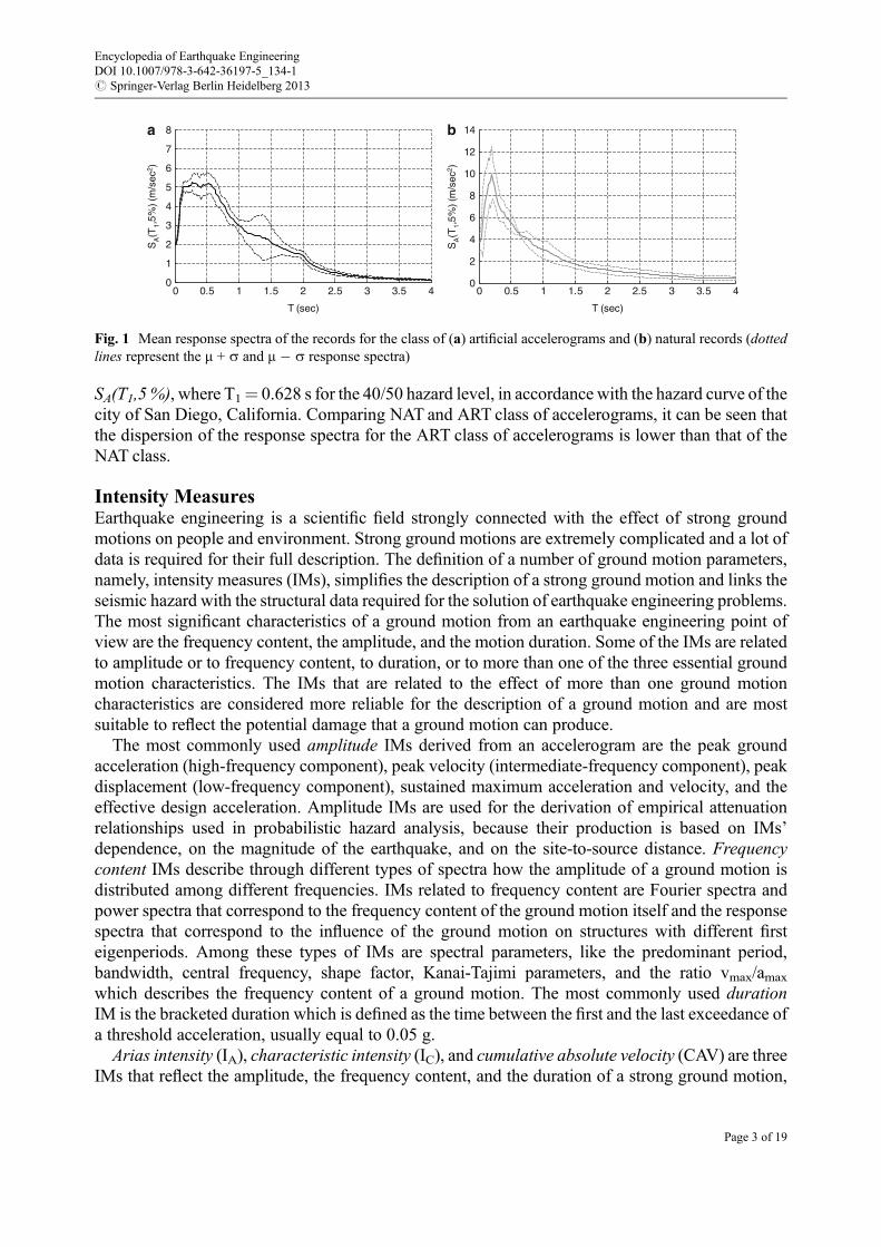
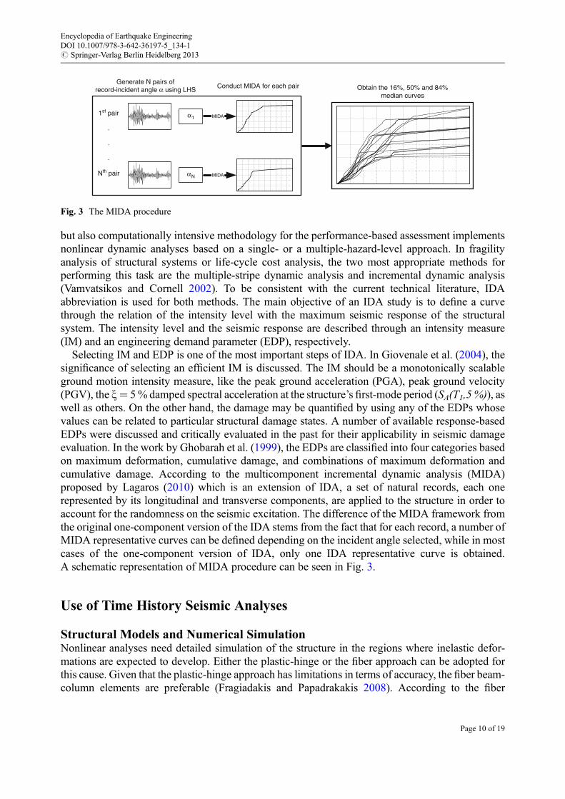
Selecting IM and EDP is one of the most important steps of IDA. In Giovenale et al. (2004), thesignificance of selecting an efficient IM is discussed. The IM should be a monotonically scalableground motion intensity measure, like the peak ground acceleration (PGA), peak ground velocity(PGV), the x¼ 5% damped spectral acceleration at the structure’s first-mode period (SA(T1,5 %)), aswell as others. On the other hand, the damage may be quantified by using any of the EDPs whosevalues can be related to particular structural damage states. A number of available response-basedEDPs were discussed and critically evaluated in the past for their applicability in seismic damageevaluation. In the work by Ghobarah et al. (1999), the EDPs are classified into four categories basedon maximum deformation, cumulative damage, and combinations of maximum deformation andcumulative damage. According to the multicomponent incremental dynamic analysis (MIDA)proposed by Lagaros (2010) which is an extension of IDA, a set of natural records, each onerepresented by its longitudinal and transverse components, are applied to the structure in order toaccount for the randomness on the seismic excitation. The difference of the MIDA framework fromthe original one-component version of the IDA stems from the fact that for each record, a number ofMIDA representative curves can be defined depending on the incident angle selected, while in mostcases of the one-component version of IDA, only one IDA representative curve is obtained.A schematic representation of MIDA procedure can be seen in Fig. 3.

Use of Time History Seismic Analyses

Structural Models and Numerical SimulationNonlinear analyses need detailed simulation of the structure in the regions where inelastic defor-mations are expected to develop. Either the plastic-hinge or the fiber approach can be adopted forthis cause. Given that the plastic-hinge approach has limitations in terms of accuracy, the fiber beam-column elements are preferable (Fragiadakis and Papadrakakis 2008). According to the fiber

Generate N pairs ofrecord-incident angle α using LHS

1st pair

Nth pair

α1

αN

.

.

.

MIDA

MIDA

Conduct MIDA for each pair Obtain the 16%, 50% and 84%median curves

Fig. 3 The MIDA procedure


of 19

approach, every beam-column element has a number of integration sections, each divided intofibers. Each fiber in the section can be assigned concrete, structural steel, or reinforcing bar materialproperties. The sections are located either at the center of the element or at its Gaussian integrationpoints. The main advantage of the fiber approach is that every fiber has a simple uniaxial materialmodel allowing an easy and efficient implementation of the inelastic behavior. This approach isconsidered to be suitable for inelastic beam-column elements under dynamic loading and providesa reliable solution compared to other formulations. However, it results to higher computationaldemands in terms of memory storage and CPU time. When a displacement-based formulation isadopted, the discretization should be adaptive with a dense mesh at the joints and a single elasticelement for the remaining part of the member. On the other hand, force-based fiber elements allowmodeling a member with a single beam-column element.

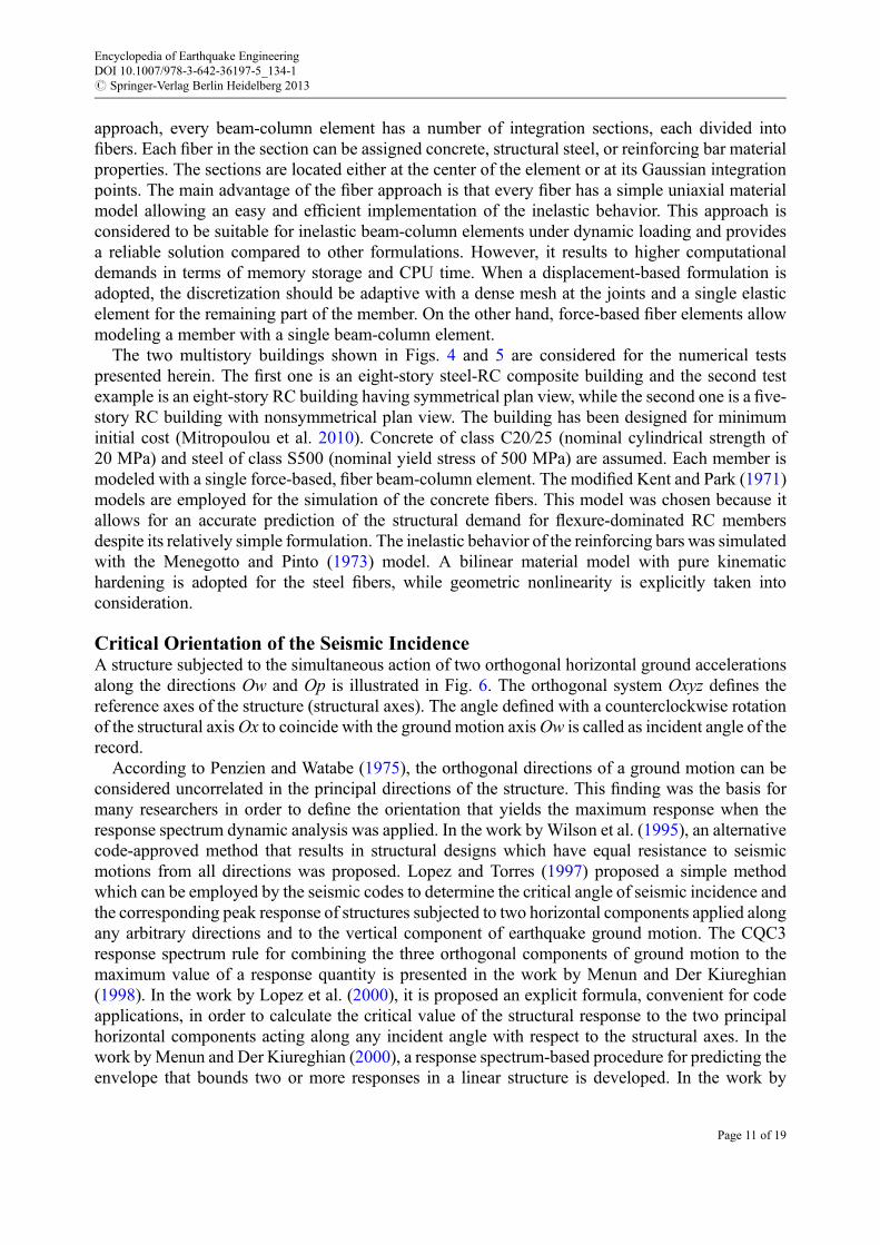
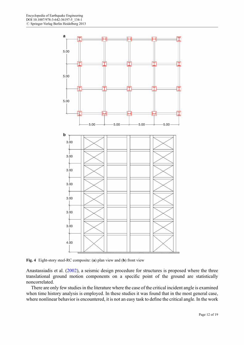
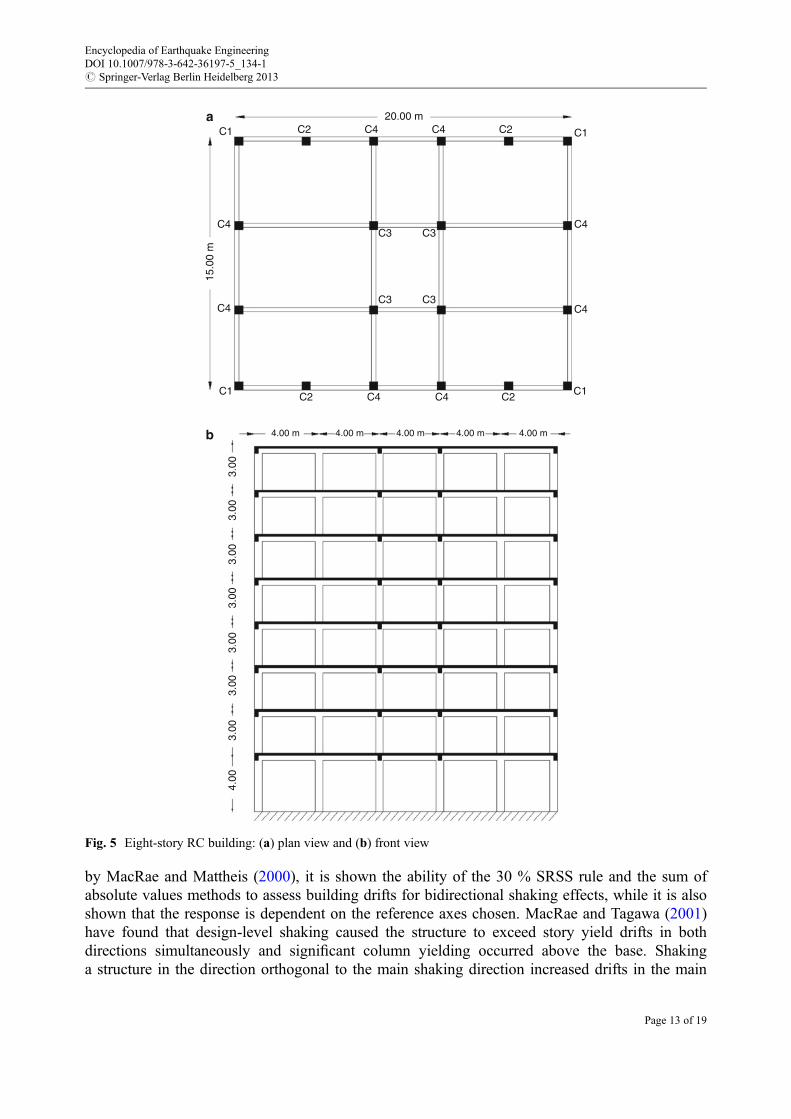
The two multistory buildings shown in Figs. 4 and 5 are considered for the numerical testspresented herein. The first one is an eight-story steel-RC composite building and the second testexample is an eight-story RC building having symmetrical plan view, while the second one is a five-story RC building with nonsymmetrical plan view. The building has been designed for minimuminitial cost (Mitropoulou et al. 2010). Concrete of class C20/25 (nominal cylindrical strength of20 MPa) and steel of class S500 (nominal yield stress of 500 MPa) are assumed. Each member ismodeled with a single force-based, fiber beam-column element. The modified Kent and Park (1971)models are employed for the simulation of the concrete fibers. This model was chosen because itallows for an accurate prediction of the structural demand for flexure-dominated RC membersdespite its relatively simple formulation. The inelastic behavior of the reinforcing bars was simulatedwith the Menegotto and Pinto (1973) model. A bilinear material model with pure kinematichardening is adopted for the steel fibers, while geometric nonlinearity is explicitly taken intoconsideration.

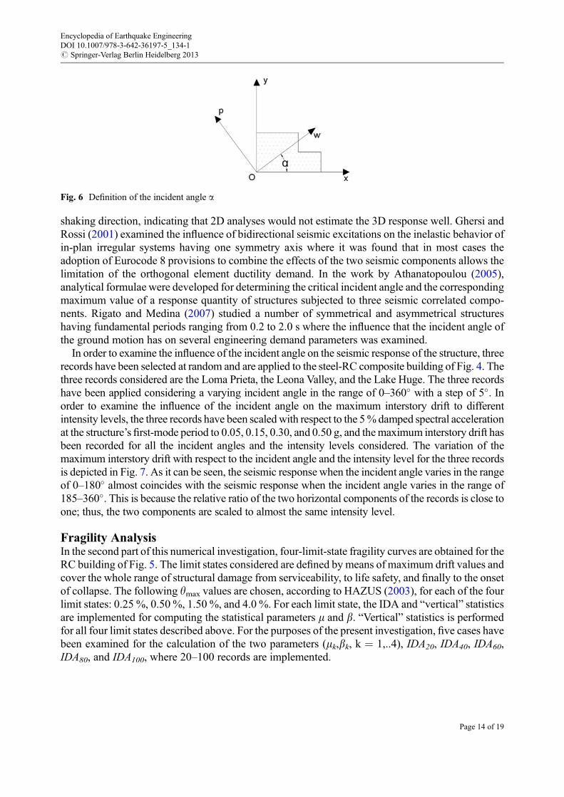
Critical Orientation of the Seismic IncidenceA structure subjected to the simultaneous action of two orthogonal horizontal ground accelerationsalong the directions Ow and Op is illustrated in Fig. 6. The orthogonal system Oxyz defines thereference axes of the structure (structural axes). The angle defined with a counterclockwise rotationof the structural axisOx to coincide with the ground motion axisOw is called as incident angle of therecord.

According to Penzien and Watabe (1975), the orthogonal directions of a ground motion can beconsidered uncorrelated in the principal directions of the structure. This finding was the basis formany researchers in order to define the orientation that yields the maximum response when theresponse spectrum dynamic analysis was applied. In the work byWilson et al. (1995), an alternativecode-approved method that results in structural designs which have equal resistance to seismicmotions from all directions was proposed. Lopez and Torres (1997) proposed a simple methodwhich can be employed by the seismic codes to determine the critical angle of seismic incidence andthe corresponding peak response of structures subjected to two horizontal components applied alongany arbitrary directions and to the vertical component of earthquake ground motion. The CQC3response spectrum rule for combining the three orthogonal components of ground motion to themaximum value of a response quantity is presented in the work by Menun and Der Kiureghian(1998). In the work by Lopez et al. (2000), it is proposed an explicit formula, convenient for codeapplications, in order to calculate the critical value of the structural response to the two principalhorizontal components acting along any incident angle with respect to the structural axes. In thework byMenun and Der Kiureghian (2000), a response spectrum-based procedure for predicting theenvelope that bounds two or more responses in a linear structure is developed. In the work by


of 19

Anastassiadis et al. (2002), a seismic design procedure for structures is proposed where the threetranslational ground motion components on a specific point of the ground are statisticallynoncorrelated.

There are only few studies in the literature where the case of the critical incident angle is examinedwhen time history analysis is employed. In these studies it was found that in the most general case,where nonlinear behavior is encountered, it is not an easy task to define the critical angle. In the work

5.00

5.00

3.00

3.00

3.00

3.00

3.00

3.00

3.00

4.00

5.00 5.00 5.00

5.00

5.00

a

b

Fig. 4 Eight-story steel-RC composite: (a) plan view and (b) front view


of 19

by MacRae and Mattheis (2000), it is shown the ability of the 30 % SRSS rule and the sum ofabsolute values methods to assess building drifts for bidirectional shaking effects, while it is alsoshown that the response is dependent on the reference axes chosen. MacRae and Tagawa (2001)have found that design-level shaking caused the structure to exceed story yield drifts in bothdirections simultaneously and significant column yielding occurred above the base. Shakinga structure in the direction orthogonal to the main shaking direction increased drifts in the main

3.00

C1

C1a

b

C4

C4

15.0

0 m

C1C2 C2C4

C3

C3 C3

C3

C4

C2 C2C420.00 m

C4

C4

C4

C1

4.00 m 4.00 m 4.00 m 4.00 m 4.00 m

3.00

3.00

3.00

3.00

3.00

3.00

4.00

Fig. 5 Eight-story RC building: (a) plan view and (b) front view


of 19

shaking direction, indicating that 2D analyses would not estimate the 3D response well. Ghersi andRossi (2001) examined the influence of bidirectional seismic excitations on the inelastic behavior ofin-plan irregular systems having one symmetry axis where it was found that in most cases theadoption of Eurocode 8 provisions to combine the effects of the two seismic components allows thelimitation of the orthogonal element ductility demand. In the work by Athanatopoulou (2005),analytical formulae were developed for determining the critical incident angle and the correspondingmaximum value of a response quantity of structures subjected to three seismic correlated compo-nents. Rigato and Medina (2007) studied a number of symmetrical and asymmetrical structureshaving fundamental periods ranging from 0.2 to 2.0 s where the influence that the incident angle ofthe ground motion has on several engineering demand parameters was examined.

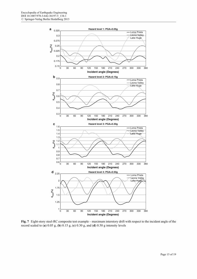
In order to examine the influence of the incident angle on the seismic response of the structure, threerecords have been selected at random and are applied to the steel-RC composite building of Fig. 4. Thethree records considered are the Loma Prieta, the Leona Valley, and the Lake Huge. The three recordshave been applied considering a varying incident angle in the range of 0–360� with a step of 5�. Inorder to examine the influence of the incident angle on the maximum interstory drift to differentintensity levels, the three records have been scaledwith respect to the 5% damped spectral accelerationat the structure’s first-mode period to 0.05, 0.15, 0.30, and 0.50 g, and themaximum interstory drift hasbeen recorded for all the incident angles and the intensity levels considered. The variation of themaximum interstory drift with respect to the incident angle and the intensity level for the three recordsis depicted in Fig. 7. As it can be seen, the seismic response when the incident angle varies in the rangeof 0–180� almost coincides with the seismic response when the incident angle varies in the range of185–360�. This is because the relative ratio of the two horizontal components of the records is close toone; thus, the two components are scaled to almost the same intensity level.

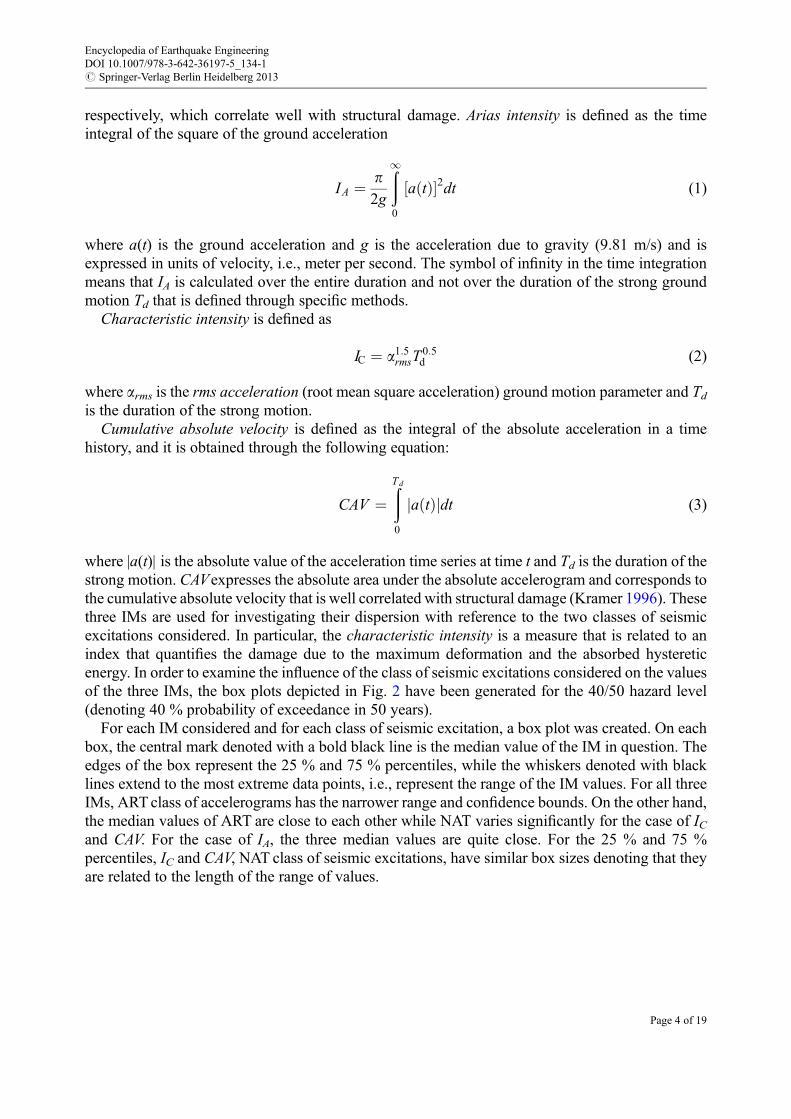
Fragility AnalysisIn the second part of this numerical investigation, four-limit-state fragility curves are obtained for theRC building of Fig. 5. The limit states considered are defined by means of maximum drift values andcover the whole range of structural damage from serviceability, to life safety, and finally to the onsetof collapse. The following ymax values are chosen, according to HAZUS (2003), for each of the fourlimit states: 0.25 %, 0.50 %, 1.50 %, and 4.0 %. For each limit state, the IDA and “vertical” statisticsare implemented for computing the statistical parameters m and b. “Vertical” statistics is performedfor all four limit states described above. For the purposes of the present investigation, five cases havebeen examined for the calculation of the two parameters (mk,bk, k ¼ 1,..4), IDA20, IDA40, IDA60,IDA80, and IDA100, where 20–100 records are implemented.

Fig. 6 Definition of the incident angle a


of 19

0.15

0.175

0.2

0.225

0.25

0.275

0.3

0.325

0 30 60 90 120 150 180 210 240 270 300 330 360

q max

(%)

Incident angle (Degrees)

Hazard level 1: PGA=0.05gLoma PrietaLeona ValleyLake Huge

q max

(%)

0.3

0.4

0.5

0.6

0.7

0.8

0.9

0 30 60 90 120 150 180 210 240 270 300 330 360



q max

(%)

0.6

0.7

0.8

0.9

1

1.1

1.2

1.3

1.4

1.5

1.6

0 30 60 90 120 150 180 210 240 270 300 330 360


Hazard level 3: PGA=0.30g

Loma PrietaLeona ValleyLake Huge

q max

(%)

1

1.25

1.5

1.75

2

2.25

0 30 60 90 120 150 180 210 240 270 300 330 360



a

b

c

d

Fig. 7 Eight-story steel-RC composite test example –maximum interstory drift with respect to the incident angle of therecord scaled to (a) 0.05 g, (b) 0.15 g, (c) 0.30 g, and (d) 0.50 g intensity levels


of 19

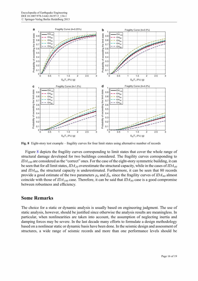
Figure 8 depicts the fragility curves corresponding to limit states that cover the whole range ofstructural damage developed for two buildings considered. The fragility curves corresponding toIDA100 are considered as the “correct” ones. For the case of the eight-story symmetric building, it canbe seen that for all limit states, IDA20 overestimate the structural capacity, while in the cases of IDA40

and IDA60, the structural capacity is underestimated. Furthermore, it can be seen that 80 recordsprovide a good estimate of the two parameters mk and bk, since the fragility curves of IDA80 almostcoincide with those of IDA100 case. Therefore, it can be said that IDA80 case is a good compromisebetween robustness and efficiency.

Some Remarks

The choice for a static or dynamic analysis is usually based on engineering judgment. The use ofstatic analysis, however, should be justified since otherwise the analysis results are meaningless. Inparticular, when nonlinearities are taken into account, the assumption of neglecting inertia anddamping forces may be severe. In the last decade many efforts to formulate a design methodologybased on a nonlinear static or dynamic basis have been done. In the seismic design and assessment ofstructures, a wide range of seismic records and more than one performance levels should be

0 0.5 1 1.5 2 2.5 30

0.1

0.2

0.3

0.4

0.5

0.6

0.7

0.8

0.9

a b

c d

1

SA(T1,5%) (g)

0 0.5 1 1.5 2 2.5 3

SA(T1,5%) (g)

0 0.5 1 1.5 2 2.5 3

SA(T1,5%) (g)

0 0.5 1 1.5 2 2.5 3

SA(T1,5%) (g)

Pro

babi

lity

of e

xcee

ding

the

limit

stat

e

0

0.1

0.2

0.3

0.4

0.5

0.6

0.7

0.8

0.9

1

Pro

babi

lity

of e

xcee

ding

the

limit

stat

e

0

0.1

0.2

0.3

0.4

0.5

0.6

0.7

0.8

0.9

1

Pro

babi

lity

of e

xcee

ding

the

limit

stat

e

0

0.1

0.2

0.3

0.4

0.5

0.6

0.7

0.8

0.9

1

Pro

babi

lity

of e

xcee

ding

the

limit

stat

e

Fragility Curve (θ=0.25%)

IDA100IDA80

IDA60IDA40IDA20

Fragility Curve (θ=0.5%)

Fragility Curve (θ=1.5%) Fragility Curve (θ=4.0%)

IDA100IDA80

IDA60IDA40IDA20

IDA100IDA80

IDA60IDA40IDA20

IDA100IDA80

IDA60IDA40IDA20

Fig. 8 Eight-story test example – fragility curves for four limit states using alternative number of records


of 19

considered in order to take into account the uncertainties that the seismic hazard introduces intoa performance-based seismic assessment or design problem. In the construction industry, decisionmaking for structural systems situated in seismically active regions requires consideration of the costof damage and other losses resulting from earthquakes which may occur during the life span of thestructures. In this entry an overview of the time history seismic analysis procedures is providedalong with indicative application of such procedures.

Summary

In the case of design or assessment purposes, the seismic capacity of the structural system should becomputed for different seismic hazard levels by means of linear or nonlinear time history seismicanalyses using a number of properly selected groundmotions. The selection of the groundmotions playsan important role in the efficiency and accuracy of the design or assessment procedure. In this entry, weprovide an overview of the time history seismic analysis applied for design and assessment purposes.

Cross-References

▶Analytic Fragility and Limit States [P(EDP|IM)]: Nonlinear Dynamic Procedures▶Assessment of Existing Structures Using Response History Analysis▶ Incremental Dynamic Analysis▶Nonlinear Dynamic Seismic Analysis▶ Seismic Hazards: Ground Shaking▶ Selection of Ground Motions for Time-History Analyses

References

Anastassiadis K, Avramidis I, Panetsos P (2002) Concurrent design forces in structures under three-component orthotropic seismic excitation. Earthq Spectra 18:1–17

ASCE (2007) Seismic rehabilitation of existing buildings. ASCE/SEI Standard 41-06. AmericanSociety of Civil Engineers, Reston

ASCE/SEI (2010) Minimum design loads for buildings and other structures. ASCE/SEI Standard07-10. American Society of Civil Engineers, Reston

Athanatopoulou AM (2005) Critical orientation of three correlated seismic components. Eng Struct27(2):301–312

CEN (2005) Eurocode 8: design of structures for earthquake resistance. EN 1998. EuropeanCommittee for Standardisation, Brussels

Chopra AK, Goel RK (2002) A modal pushover analysis procedure for estimating seismic demandsfor buildings. Earthq Eng Struct Dyn 31(3):561–582

Fajfar P (2000) A nonlinear analysis method for performance-based seismic design. Earthq Spectra16(3):573–592


of 19







FEMA (2003) HAZUS-MH MR1, Multi-hazard loss estimation methodology earthquake model.National Institute of Building Sciences, Washington, DC

Fib (2012) Probabilistic performance-based seismic design. Bulletin 68. International Federation ofStructural Concrete, Lausanne

Fragiadakis M, Papadrakakis M (2008) Modelling, analysis and reliability of seismically excitedstructures: computational issues. Int J Comput Methods 5(4):483–511

Gasparini DA, Vanmarke EH (1976) Simulated earthquake motions compatible with prescribedresponse spectra. Massachusetts Institute of Technology (MIT), Department of Civil Engineering,Publication No. R76-4, Cambridge, MA

Ghersi A, Rossi PP (2001) Influence of bi-directional ground motions on the inelastic response ofone-storey in-plan irregular systems. Eng Struct 23(6):579–591

Ghobarah A, Abou-Elfath H, Biddah A (1999) Response-based damage assessment of structures.Earthq Eng Struct Dyn 28(1):79–104

Giovenale P, Cornell CA, Esteva L (2004) Comparing the adequacy of alternative ground motionintensity measures for the estimation of structural responses. Earthq Eng Struct Dyn33(8):951–979

Houbolt JC (1950) A recurrence matrix solution for the dynamic response of elastic aircraft.J Aeronaut Sci 17:540–550

Kent DC, Park R (1971) Flexural members with confined concrete. J Struct Div 97(7):1969–1990Kramer SL (1996) Geotechnical earthquake engineering. Prentice Hall, Upper Saddle RiverLagaros ND (2010) Multicomponent incremental dynamic analysis considering variable incident

angle. J Struct Infrastruct Eng 6(1–2):77–94Lopez OA, Torres R (1997) The critical angle of seismic incidence and the maximum structural

response. Earthq Eng Struct Dyn 26:881–894Lopez OA, Chopra AK, Hernandez JJ (2000) Critical response of structures to multicomponent

earthquake excitation. Earthq Eng Struct Dyn 29:1759–1778MacRae GA, Mattheis J (2000) Three-dimensional steel building response to near-fault motions.

J Struct Eng 126(1):117–126MacRae GA, Tagawa H (2001) Seismic behaviour of 3D steel moment frame with biaxial columns.

J Struct Eng 127(5):490–497Menegotto M, Pinto PE (1973) Method of analysis for cyclically loaded reinforced concrete plane

frames including changes in geometry and non-elastic behaviour of elements under combinednormal force and bending. In: Proceedings, IABSE symposium on resistance and ultimatedeformability of structures acted on by well defined repeated loads, Zurich, Switzerland,pp 15–22

Menun C, Der Kiureghian A (1998) A replacement for the 30 %, 40 % and SRSS rules formulticomponent seismic analysis. Earthq Spectra 14(1):153–163

Menun C, Der Kiureghian A (2000) Envelopes for seismic response vectors. I: theory. J Struct Eng126:467–473

Mitropoulou Ch Ch, Lagaros ND, Papadrakakis M (2010) Economic building design based onenergy dissipation: a critical assessment. Bull Earthq Eng 8(6):1375–1396

Newmark NM (1959) A method of computation for structural dynamics. ASCE J Eng Mech Div85:67–94


of 19

Pacific Earthquake Engineering Research (PEER) (2012) http://peer.berkeley.edu/smcat/search.html/. Accessed Nov 2012

Penzien J, Watabe M (1975) Characteristics of 3-dimensional earthquake ground motions. EarthqEng Struct Dyn 3(4):365–373

Rigato AB, Medina RA (2007) Influence of angle of incidence on seismic demands for inelasticsingle-storey structures subjected to bi-directional groundmotions. Eng Struct 29(10):2593–2601

Vamvatsikos D, Cornell CA (2002) Incremental dynamic analysis. Earthq Eng Struct Dyn31(3):491–514

Wilson EL, Farhoomand I, Bathe KJ (1973) Nonlinear dynamic analysis of complex structures.Earthq Eng Struct Dyn 1:241–252

Wilson EL, Suharwardy A, Habibullah A (1995) A clarification of the orthogonal effects in a three-dimensional seismic analysis. Earthq Spectra 11(4):659–666


of 19

http://peer.berkeley.edu/smcat/search.html/

http://peer.berkeley.edu/smcat/search.html/

encyclopedia of earthquake engineering || time history seismic analysis

Documents