Encoder-Decoder Approach to Predict AirportOperational Runway Configuration

A case study for Amsterdam Schiphol airport

Ramon Dalmau & Floris HerremaNetwork (NET) and Airport (APT) Research Units

EUROCONTROL Experimental Centre (EEC)Bretigny-Sur-Orge, France

Abstract—The runway configuration of an airport is the com-bination of runways that are active for arrivals and departuresat any time. The runway configuration has a major influenceon the capacity of the airport, taxiing times, the occupation ofparking stands and taxiways, as well as on the managementof traffic in the airspace surrounding the airport. The runwayconfiguration of a given airport may change several times duringthe day, depending on the weather, air traffic demand and noiseabatement rules, among other factors. This paper proposes anencoder-decoder model that is able to predict the future runwayconfiguration sequence of an airport several hours upfront. Incontrast to typical rule-based approaches, the proposed model isgeneric enough to be applied to any airport, since it only requiresthe past runway configuration history and the forecast trafficdemand and weather in the prediction horizon. The performanceof the model is assessed for the Amsterdam Schiphol Airportusing three years of traffic, weather and runway use data.

Index Terms—runway configuration, machine learning

I. INTRODUCTION

Runways enable aircraft to take-off and landing. As such, atmajor airports, the capacity of runways is the most restrictingelement in considering total airport operations. Major airportshave several runways in order to accommodate a large amountof aircraft movements. For instance, the Hartsfield-JacksonAtlanta International Airport, which is the busiest airport in theworld with more than 107 million passengers in 2018 utilises 5runways. The number of runways of an airport, however, doesnot only depend on the volume of traffic. Runways may bereserved for certain type of traffic, wind directions, visibilityconditions, time periods, or for noise abatement procedures.

It should be noted that not all runways of an airport are usedsimultaneously. The planned combination of runways that areactive at any time is called the ”runway configuration”. Forairports with multiple runways the number of possible con-figurations may be large. For instance, Amsterdam SchipholAirport (EHAM) has 6 runways, which could be combined inmore than 100 different ways. In practise, however, only 2 or3 are used simultaneously. During daily time in summer, only8 runway configurations are used 70% of the time in average1.

The runway configuration greatly influences the capacity ofthe airport. In addition, the in and out taxi times and thus

1https://ext.eurocontrol.int/airport corner public/EHAM

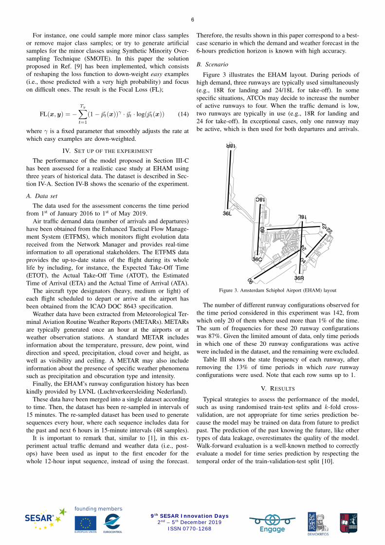
the duration of the flights from off-block time to on-block,also depend on the runways that are used to take-off and landfrom/to the origin and destination airports, respectively. Forinstance, aircraft using the 18R/36L runway of EHAM (seeFig. 3), located to reduce the noise impact on the surroundingcommunities, have a 20-minute taxi to/from the terminal,while for other runways, the taxi-time is about 10 minutes.The runway configuration also has a major impact on theoccupation of parking stands and taxiways, as well as on themanagement of traffic in the airspace surrounding the airport.

At present, the selection of runway configuration is mainlybased on human experience. Air Traffic Controllers (ATCOs)examine several factors to determine the best sequence of run-way configurations to be used in the next hours. For instance, itis well known that wind speed and wind direction influence thechoice of the runway configuration since cross-winds (relativeto the direction of that runway) exceeding a threshold maynot be adequate to take-off and landing. Moreover, certainrunways may be prohibited under poor visibility conditionsdue to unqualified instrumentation. In addition to winds andvisibility, a runway may be also not operable due to highlyintense precipitation or icing conditions. Last but not least,extremely hot temperatures can make take-off impossible forcertain aircraft because of insufficient lift force. The schedulednumber of arrivals and departures for the next hours as well asthe aircraft wake categories are also expected to have a greatimpact when deciding which runways to use at a given time.

Unfortunately, it is difficult to represent the criteria con-sidered by the ATCOs to determine the runway configurationgiven the influencing factors with generic rule-based models,and thus it is difficult to accurately predict the future runwayconfiguration (and all the variables that depend on it). More-over, each airport may implement different rules, meaning thatcreating a generic rule-based model might be unfeasible. Forinstance, at EHAM, weather is the main factor considered byATCOs when selecting the configuration1. The environmental(in particular noise) rules for the use of runways, however,also play a role in determining the runway configuration.

Several works have attempted to predict the future runwayconfiguration. For instance, reference [1] proposed a discrete-choice model of the configuration selection process from em-

9th SESAR Innovation Days 2nd – 5th December 2019

ISSN 0770-1268

pirical data. Results showed that, if the actual traffic demandand weather conditions where known 3 hours in advance, themodel could predict the runway configuration at La Guardiaand San Francisco airports with an accuracy of 82% and 85%,respectively. More recently, Ref. [2] proposed an ArtificialNeural Network (ANN) architecture that uses similar datato predict the runway configuration and the correspondingcapacity. Results for predictions one hour ahead showed apromising predictive power. The dataset used to train andevaluate the model, however, comprised only 24 hours.

This paper proposes an encoder-decoder model inspired bysequence to sequence techniques to predict the runway con-figuration sequence of an airport every 15 min in an horizonof 6 hours. The model takes as inputs the observed weatherand traffic demand in the near past, as well as the weatherand traffic demand forecast in the 6-hours prediction horizon.This information is combined with the recently used runwayconfiguration history to perform the sequence prediction. Theperformance of the model is assessed for EHAM using threeyears of traffic, weather and runway use data.

II. SEQUENCE TO SEQUENCE (SEQ2SEQ) MODELS

Note that throughout this paper, and as a general rule,scalars and vectors are denoted either with lower or upper caseletters, e.g., a or A. Vectors are denoted with the conventionaloverhead arrow, e.g., ~a; while sequences use the same font butin bold, .e.g, a. Sets are denoted using calligraphic fonts, e.g.,A; while matrices use the same font but in bold, e.g., A.

Seq2seq models lie behind numerous applications suchas neural machine translation, text summarisation, speechrecognition, video captioning, online chat-bots and other caseswhere it is desirable to generate a sequence from another [4].

The goal of a seq2seq model is to find the output se-quence y = (~y1, ~y2, . . . , ~yTy

) in <ny that maximizes theconditional probability of y given the input sequence x =(~x1, ~x2, . . . , ~xTx

) in <nx , i.e., argmaxyp(y|x). Tx and Ty arethe length of the input and output sequences, respectively.

A. Basic encoder-decoder

Conventional seq2seq models used in many applicationsconsist of two parts: the encoder and the decoder. The roleof the encoder is to condense the information of the inputsequence x into a vector of a fixed length ~c, commonly knownas context. The context is used to condition the decoder, whichgenerates the output sequence y that maximises p(y|x). Thearchitecture of a basic encoder-decoder is shown in Fig. 1a.

The usual approach is to use a Recurrent Neural Network(RNN) as encoder. Roughly speaking, a RNN has a loopingmechanism that allows important information to flow fromone time step to the next one. This information is stored inthe hidden state of the RNN, ~ht ∈ <nh . At each time step tthe RNN takes the inputs vector and updates its hidden state:

~ht = Recurrentφh,ψh,nh

(~ht−1, ~xt

), (1)

where Recurrent is a nonlinear function that depends on theRNN type. In Eq. (1), φh and ψh are the activation and

recurrent activation functions, respectively. For instance, fora vanilla RNN the update is typically performed as [5]:

~ht = tanh(Whh

~ht−1 +Whx~xt +~bh

), (2)

where Whh ∈ <nh×nh and Whx ∈ <nh×nx are trainablematrices and ~bh ∈ <nh is the (also trainable) bias vector.Note that at t = 1 the hidden state depends on the first inputsvector ~x1 as well as the initial hidden state ~h0. The defaultapproach consists of initialising the hidden state with zeros(i.e., ~h0 = ~0). This strategy often works well for seq2seq.

Vanilla RNNs, frequently have the problem of vanishinggradients which, negatively influences the learning of longsequences. To solve vanishing gradients a popular way is touse LSTM (Long Short Term Memory) [6] or Gated RecurrentUnit (GRU) [7].

Generally speaking, the context vector that conditions thedecoder to generate y could be any nonlinear function q ofthe whole sequence of hidden states generated by the encoder:

~c = q (h) = q(~h1,~h2, . . . ,~hTx

). (3)

The most basic encoder-decoder model, however, simplyuses the last hidden state as context vector, i.e, ~c = ~hTx

.The decoder component is another RNN trained to predict

the next output ~yt given the context vector ~c and all thepreviously predicted outputs ~y1, . . . , ~yt−1. In other words, thedecoder defines a probability over the sequence y by decom-posing the joint probability into the ordered conditionals:

p (y|x) =Ty∏t=1

p (~yt|~y<t,~c) =Ty∏t=1

p (~yt|~y1, . . . , ~yt−1,~c) , (4)

where the context vector is an implicit function of x throughEq. (3). The conditional probability of ~yt is computed as:

~pt = p(~yt|~y<t,~c) = Denseφd,ny(~st) , (5)

where a fully-connected dense layer of n units and activationfunction φ is defined as the operation that applied to any vectorof inputs ~x ∈ <m generates the output ~y ∈ <n according to:

~y = Denseφ,n(~x) = φ(W~x+~b

), (6)

where W ∈ <n×m is a weighting matrix, and ~b ∈ <n is thebias vector. Both W and ~b are parameters to be trained.

In Eq. (5), ~st ∈ <ns is the hidden state of the decoder’sRNN, which can be computed similar to Eq. (1):

~st = Recurrentφs,ψs,ns(~st−1, ~yt−1) (7)

As for the encoder, in most practical applications thedecoder is a GRU or LSTM. In the basic encoder-decoder ar-chitecture (see Fig.1a), the context vector is only used once toinitialize the hidden state of the decoder (i.e., ~s0 = ~c = ~hTx

).The decoder behaves differently during training and infer-

ence (prediction of unseen data). During training, the ground

2

9th SESAR Innovation Days 2nd – 5th December 2019

ISSN 0770-1268

... ...

......

...

<START>

Encoder Decoder

Inputs RNN OutputsDenseAlignment Dot productConcatenation

(a) Basic

... ...

......

...

<START>

Encoder Decoder

Attention

...

...

...

(b) With Luong [3] attention

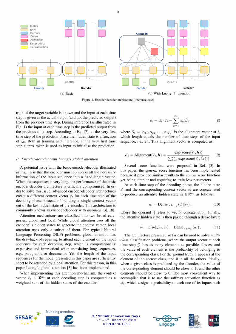
Figure 1. Encoder-decoder architecture (inference case)

truth of the target variable is known and the input at each timestep is given as the actual output (and not the predicted output)from the previous time step. During inference (as illustrated inFig. 1) the input at each time step is the predicted output fromthe previous time step. According to Eq. (7), at the very firsttime step of the prediction phase the hidden state is a functionof ~y0. Both in training and inference, at the very first timestep a start token is used as input to initialise the prediction.

B. Encoder-decoder with Luong’s global attention

A potential issue with the basic encoder-decoder illustratedin Fig. 1a is that the encoder must compress all the necessaryinformation of the input sequence into a fixed-length vector.When the sequences is very long, the performance of the basicencoder-decoder architecture is critically compromised. In or-der to solve this issue, advanced encoder-decoder architecturescreate a different context vector ~ct for each time step of thedecoding phase, instead of building a single context vectorout of the last hidden state of the encoder. This architecture iscommonly known as encoder-decoder with attention [3], [8].

Attention mechanisms are classified into two broad cate-gories: global and local. While global attention uses all theencoder’ s hidden states to generate the context vector, localattention uses only a subset of them. For typical NaturalLanguage Processing (NLP) problems, global attention hasthe drawback of requiring to attend each element on the inputsequence for each decoding step, which is computationallyexpensive and impractical when translating long sequences,e.g., paragraphs or documents. Yet, the length of the inputsequences for the model presented in this paper are sufficientlyshort to be attended by global attention. For this reason, in thispaper Luong’s global attention [3] has been implemented.

When implementing this attention mechanism, the contextvector ~ct ∈ <nh at each decoding step is computed as aweighted sum of the hidden states of the encoder:

~ct = ~αt · h =

Tx∑k=1

αtk~hk, (8)

where ~αt = [αt1, αt2, . . . , αtTx] is the alignment vector at t,

which length equals the number of time steps of the inputsequence, i.e., Tx. This alignment vector is computed as:

~αt = Alignment(~st,h) =exp(score(~st,h))∑Tx

k=1 exp(score(~st,~hk))). (9)

Several score functions were proposed in Ref. [3]. Inthis paper, the general score function has been implementedbecause it provided similar results to the concat score functionyet being simpler and requiring to train less parameters.

At each time step of the decoding phase, the hidden state~st and the corresponding context vector ~ct are concatenatedto produce an attentive hidden state ~at ∈ <na as follows:

~at = Densetanh,na(~ct||~st) , (10)

where the operand || refers to vector concatenation. Finally,the attentive hidden state is then passed through a dense layer:

~pt = p(~yt|~y<t,~ct) = Denseφd,ny (~at) . (11)

The architecture presented so far can be used to solve multi-class classification problems, where the output vector at eachtime step ~yt has as many elements as possible classes, andthe value of each element is the probability of belonging tothe corresponding class. For the ground truth, 1 appears at theelement of the correct class, and 0 in all the others. Ideally,when a given class is predicted by the decoder, the value ofthe corresponding element should be close to 1, and the otherelements should be close to 0. The most convenient way toaccomplish that is to use the softmax activation function asφd, which assigns a probability to each one of its inputs such

3

9th SESAR Innovation Days 2nd – 5th December 2019

ISSN 0770-1268

that∑~pt = 1. Accordingly, the probability associated to a

class is not independent from that of the others.The encoder-decoder is typically trained to minimize the

cross-entropy (CE), calculated independently for each outputvector in the sequence and then summed up. For a giventraining example composed by the input and output sequences:

CE(x,y) = −Ty∑t=1

~yt · log(~pt(x)), (12)

where ~yt is the ground truth and ~pt is the probability predictedby the model given x. In binary classification, where thenumber of classes is 2, each element in the output sequenceis a scalar, i.e., y = (y1, y2, . . . , yTy

) in <, which probabilityis predicted by using sigmoid activation function as φd [5].

III. PROPOSED APPROACH

As mentioned in Section I, ATCOs select runway config-uration based on many factors, including weather conditions,traffic demand, and noise regulations, which might depend inturn on the hour of the day, for instance. The aim of thisstudy is to assess the feasibility of a data-driven model trainedon historical data capable to predict the runway configurationseveral hours ahead using some of these features as input.

The most straightforward way to accomplish that consistsof feeding a feed-forward neural network with the aforemen-tioned features at a particular time and predict the instanta-neous runway configuration. Most probably, ATCOs do notonly look these features at a given time to make a decision,but also take into account their evolution on a prolonged timeinterval (e.g., several hours). Therefore, the first hypothesis ofthe model proposed herein is that a sequence of these featuresis what drives ATCOs decisions. The second hypothesis is thatthe probability of selecting a runway configuration at a giventime is conditioned on the previous decisions in the recentpast. Taking these two hypothesis into account, an attractivemodel to capture information encoded in a sequence of inputsand generate a sequence out of this is the encoder-decoderwith attention described in Section II.

The outputs and inputs of the model are presented inSections III-A and III-B, respectively. Then, the proposedencoder-decoder architecture is described in Section III-C.

A. Outputs of the decoder

The target variable for the problem tackled in this paper canbe defined in different ways. The final choice will determinethe number and type of outputs that the decoder generates, aswell as the activation function of their last dense layer.

The most straightforward strategy consists of identifying allpossible combinations of runways, associate each one to agiven class, and solve a single-output multi-class classificationproblem. Using this approach, the output of the decoder ateach time sample is, in point of fact, a class representing thepredicted runway configuration. As discussed in Section II-B,the usual way to address multi-class classification problems isto transform the target variable to a one-hot vector, meaning

that the output of the decoder is a vector with as many ele-ments as classes (runway configurations), where each elementis the probability associated to that class. These probabilitiesare generated by a softmax function as φd and sum up to 1.

In this paper, the problem is addressed as a multi-outputmutli-class classification, where each output corresponds toa runway. The airport may have runways that are used onlyfor take-off, only landing, or that could be used for both.For the set of runways that are always used for an uniquetype of operation (Rb), the corresponding outputs are scalarbinary variables: active or inactive. For the set of runwaysthat could be used to accommodate departures and arrivals(Rm), the corresponding outputs are categorical variables withthree possible classes: take-off, landing or inactive. The way ofhandling each individual output for runways inRm is identicalto that of the single-output multi-class described above. Theoutput corresponding to each runway in Rb is a scalar whichprobability value is generated by a sigmoid activation function.

If compared to the single-output multi-class strategy, themulti-output multi-class has the advantage that if only the stateof one runway (one output) is unsatisfactorily predicted, thepenalty to the loss function is lower than if the predictions forall runways (i.e., runway configuration) are wrong.

The decoder generates the sequence of outputs, where eachoutput is the state of the corresponding runway (either a binaryscalar or a one-hot representation of a 3-class categoricalvariable), for the following 6 hours in intervals of 15 minutes.Therefore, in this model Ty = 24, and ny = |Rb|+ 3|Rm|.

B. Inputs of the encoders

The encoder-decoder model is composed by two encoders,each one receiving a different sequence of input features.

The task of the first encoder is to capture factors influencingthe choice of runway configuration sequence related to theweather and traffic demand in the near past and also in theprediction horizon. The length of the sequence fed to thisencoder is Tx = 48, with each element in the sequenceincluding the features shown in Table I over a 15-minuteinterval. Accordingly, this encoder receives information overa 12-hour period. The first 24 elements correspond to theobservations in the past 6 hours, and the remaining 24 elementsinclude the forecast over the prediction horizon (next 6 hours).

The input vector fed to this encoder at each time stepincludes weather features such as wind direction and speed,temperature and visibility; demand features such as how manydepartures of each aircraft category type are planned in thecorresponding 15-minute interval; and calendar features suchas the hour of the day. Note that some of these features arecontinuous while others are categorical (discrete). In this study,each categorical variable has been represented as a one-hotvector, yet the use of embeddings is also encouraged.

The introduction of the second encoder is motivated bythe fact that the recently used configuration sequence mightalso condition the decision of ATCOs. As such, the seconddecoder takes the known runway configuration sequence usedin the past 6 hours, also discretised in intervals of 15 minutes.

4

9th SESAR Innovation Days 2nd – 5th December 2019

ISSN 0770-1268

...

...

Attention 2

...

...

...

...

...

<current runway

configuration>Encoder 1 Decoder

...

...

...

...

Attention 1

...

...

Encoder 2

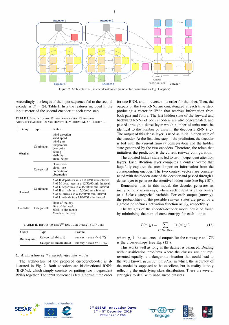
Figure 2. Architecture of the encoder-decoder (same color convention as Fig. 1 applies)

Accordingly, the length of the input sequence fed to the secondencoder is Tx = 24. Table II lists the features included in theinput vector of the second encoder at each time step.

TABLE I. INPUTS TO THE 1ST ENCODER EVERY 15 MINUTES.AIRCRAFT CATEGORIES ARE HEAVY: H, MEDIUM: M, AND LIGHT: L.

Group Type Feature

Weather

Continuous

wind directionwind speedwind gusttemperaturedew pointceilingvisibilitycloud height

Categorical

cloud covercloud typeprecipitationobscuration

DemandContinuous

# of H departures in a 15/30/60 min interval# of M departures in a 15/30/60 min interval# of L departures in a 15/30/60 min interval# of H arrivals in a 15/30/60 min interval# of M arrivals in a 15/30/60 min interval# of L arrivals in a 15/30/60 min interval

Calendar Categorical

Hour of the dayDay of the weekWeek of the monthMonth of the year

TABLE II. INPUTS TO THE 2ND ENCODER EVERY 15 MINUTES

Group Type Feature

Runway use Categorical (binary) runway r state ∀r ∈ Rb

Categorical (multi-class) runway r state ∀r ∈ Rm

C. Architecture of the encoder-decoder model

The architecture of the proposed encoder-decoder is il-lustrated in Fig. 2. Both encoders are bi-directional RNNs(BRRNs), which simply consists on putting two independentRNNs together. The input sequence is fed in normal time order

for one RNN, and in reverse time order for the other. Then, theoutputs of the two RNNs are concatenated at each time step,producing a vector in <2nh that receives information fromboth past and future. The last hidden state of the forward andbackward RNNs of both encoders are also concatenated, andpassed through a dense layer which number of units must beidentical to the number of units in the decoder’s RNN (ns).The output of this dense layer is used as initial hidden state ofthe decoder. At the first time step of the prediction, the decoderis fed with the current runway configuration and the hiddenstate generated by the two encoders. Therefore, the token thatinitialises the prediction is the current runway configuration.

The updated hidden state is fed to two independent attentionlayers. Each attention layer computes a context vector thathopefully captures the most important information from thecorresponding encoder. The two context vectors are concate-nated with the hidden state of the decoder and passed through adense layer to generate the attentive hidden state (see Eq. (10)).

Remember that, in this model, the decoder generates asmany outputs as runways, where each output is either binaryor a 3-class categorical variable. For each output (runway),the probabilities of the possible runway states are given by asigmoid or softmax activation function as φd, respectively.

The weights of the encoder-decoder model could be foundby minimising the sum of cross-entropy for each output:

L(x,y) =∑

r∈Rb∪Rm

CE(x,yr) (13)

where yr is the sequence of outputs for the runway r and CEis the cross-entropy (see Eq. (12)).

This works well as long as the dataset is balanced. Dealingwith classification problems where the classes are not rep-resented equally is a dangerous situation that could lead tothe well known accuracy paradox, in which the accuracy ofthe model is supposed to be excellent, but in reality is onlyreflecting the underlying class distribution. There are severalstrategies to deal with unbalanced datasets.

5

9th SESAR Innovation Days 2nd – 5th December 2019

ISSN 0770-1268

For instance, one could sample more minor class samplesor remove major class samples; or try to generate artificialsamples for the minor classes using Synthetic Minority Over-sampling Technique (SMOTE). In this paper the solutionproposed in Ref. [9] has been implemented, which consistsof reshaping the loss function to down-weight easy examples(i.e., those predicted with a very high probability) and focuson difficult ones. The result is the Focal Loss (FL);

FL(x,y) = −Ty∑t=1

(1− ~pt(x))γ · ~yt · log(~pt(x)) (14)

where γ is a fixed parameter that smoothly adjusts the rate atwhich easy examples are down-weighted.

IV. SET UP OF THE EXPERIMENT

The performance of the model proposed in Section III-Chas been assessed for a realistic case study at EHAM usingthree years of historical data. The dataset is described in Sec-tion IV-A. Section IV-B shows the scenario of the experiment.

A. Data set

The data used for the assessment concerns the time periodfrom 1st of January 2016 to 1st of May 2019.

Air traffic demand data (number of arrivals and departures)have been obtained from the Enhanced Tactical Flow Manage-ment System (ETFMS), which monitors flight evolution datareceived from the Network Manager and provides real-timeinformation to all operational stakeholders. The ETFMS dataprovides the up-to-date status of the flight during its wholelife by including, for instance, the Expected Take-Off Time(ETOT), the Actual Take-Off Time (ATOT), the EstimatedTime of Arrival (ETA) and the Actual Time of Arrival (ATA).

The aircraft type designators (heavy, medium or light) ofeach flight scheduled to depart or arrive at the airport hasbeen obtained from the ICAO DOC 8643 specification.

Weather data have been extracted from Meteorological Ter-minal Aviation Routine Weather Reports (METARs). METARsare typically generated once an hour at the airports or atweather observation stations. A standard METAR includesinformation about the temperature, pressure, dew point, winddirection and speed, precipitation, cloud cover and height, aswell as visibility and ceiling. A METAR may also includeinformation about the presence of specific weather phenomenasuch as precipitation and obscuration type and intensity.

Finally, the EHAM’s runway configuration history has beenkindly provided by LVNL (Luchtverkeersleiding Nederland).

These data have been merged into a single dataset accordingto time. Then, the dataset has been re-sampled in intervals of15 minutes. The re-sampled dataset has been used to generatesequences every hour, where each sequence includes data forthe past and next 6 hours in 15-minute intervals (48 samples).

It is important to remark that, similar to [1], in this ex-periment actual traffic demand and weather data (i.e., post-ops) have been used as input to the first encoder for thewhole 12-hour input sequence, instead of using the forecast.

Therefore, the results shown in this paper correspond to a best-case scenario in which the demand and weather forecast in the6-hours prediction horizon is known with high accuracy.

B. Scenario

Figure 3 illustrates the EHAM layout. During periods ofhigh demand, three runways are typically used simultaneously(e.g., 18R for landing and 24/18L for take-off). In somespecific situations, ATCOs may decide to increase the numberof active runways to four. When the traffic demand is low,two runways are typically in use (e.g., 18R for landing and24 for take-off). In exceptional cases, only one runway maybe active, which is then used for both departures and arrivals.

Figure 3. Amsterdam Schiphol Airport (EHAM) layout

The number of different runway configurations observed forthe time period considered in this experiment was 142, fromwhich only 20 of them where used more than 1% of the time.The sum of frequencies for these 20 runway configurationswas 87%. Given the limited amount of data, only time periodsin which one of these 20 runway configurations was activewere included in the dataset, and the remaining were excluded.

Table III shows the state frequency of each runway, afterremoving the 13% of time periods in which rare runwayconfigurations were used. Note that each row sums up to 1.

V. RESULTS

Typical strategies to assess the performance of the model,such as using randomised train-test splits and k-fold cross-validation, are not appropriate for time series prediction be-cause the model may be trained on data from future to predictpast. The prediction of the past knowing the future, like othertypes of data leakage, overestimates the quality of the model.Walk-forward evaluation is a well-known method to correctlyevaluate a model for time series prediction by respecting thetemporal order of the train-validation-test split [10].

6

9th SESAR Innovation Days 2nd – 5th December 2019

ISSN 0770-1268

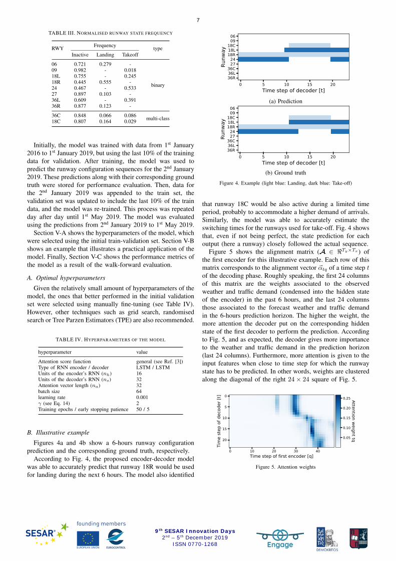
TABLE III. NORMALISED RUNWAY STATE FREQUENCY

RWY Frequency typeInactive Landing Takeoff

06 0.721 0.279 -

binary

09 0.982 - 0.01818L 0.755 - 0.24518R 0.445 0.555 -24 0.467 - 0.53327 0.897 0.103 -36L 0.609 - 0.39136R 0.877 0.123 -

36C 0.848 0.066 0.086 multi-class18C 0.807 0.164 0.029

Initially, the model was trained with data from 1st January2016 to 1st January 2019, but using the last 10% of the trainingdata for validation. After training, the model was used topredict the runway configuration sequences for the 2nd January2019. These predictions along with their corresponding groundtruth were stored for performance evaluation. Then, data forthe 2nd January 2019 was appended to the train set, thevalidation set was updated to include the last 10% of the traindata, and the model was re-trained. This process was repeatedday after day until 1st May 2019. The model was evaluatedusing the predictions from 2nd January 2019 to 1st May 2019.

Section V-A shows the hyperparameters of the model, whichwere selected using the initial train-validation set. Section V-Bshows an example that illustrates a practical application of themodel. Finally, Section V-C shows the performance metrics ofthe model as a result of the walk-forward evaluation.

A. Optimal hyperparameters

Given the relatively small amount of hyperparameters of themodel, the ones that better performed in the initial validationset were selected using manually fine-tuning (see Table IV).However, other techniques such as grid search, randomisedsearch or Tree Parzen Estimators (TPE) are also recommended.

TABLE IV. HYPERPARAMETERS OF THE MODEL

hyperparameter value

Attention score function general (see Ref. [3])Type of RNN encoder / decoder LSTM / LSTMUnits of the encoder’s RNN (nh) 16Units of the decoder’s RNN (ns) 32Attention vector length (na) 32batch size 64learning rate 0.001γ (see Eq. 14) 2Training epochs / early stopping patience 50 / 5

B. Illustrative example

Figures 4a and 4b show a 6-hours runway configurationprediction and the corresponding ground truth, respectively.

According to Fig. 4, the proposed encoder-decoder modelwas able to accurately predict that runway 18R would be usedfor landing during the next 6 hours. The model also identified

(a) Prediction

(b) Ground truth

Figure 4. Example (light blue: Landing, dark blue: Take-off)

that runway 18C would be also active during a limited timeperiod, probably to accommodate a higher demand of arrivals.Similarly, the model was able to accurately estimate theswitching times for the runways used for take-off. Fig. 4 showsthat, even if not being perfect, the state prediction for eachoutput (here a runway) closely followed the actual sequence.

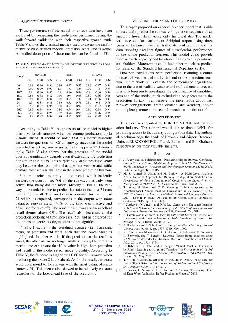
Figure 5 shows the alignment matrix (A ∈ <Ty×Tx ) ofthe first encoder for this illustrative example. Each row of thismatrix corresponds to the alignment vector ~αtq of a time step tof the decoding phase. Roughly speaking, the first 24 columnsof this matrix are the weights associated to the observedweather and traffic demand (condensed into the hidden stateof the encoder) in the past 6 hours, and the last 24 columnsthose associated to the forecast weather and traffic demandin the 6-hours prediction horizon. The higher the weight, themore attention the decoder put on the corresponding hiddenstate of the first decoder to perform the prediction. Accordingto Fig. 5, and as expected, the decoder gives more importanceto the weather and traffic demand in the prediction horizon(last 24 columns). Furthermore, more attention is given to theinput features when close to time step for which the runwaystate has to be predicted. In other words, weights are clusteredalong the diagonal of the right 24× 24 square of Fig. 5.

Figure 5. Attention weights

7

9th SESAR Innovation Days 2nd – 5th December 2019

ISSN 0770-1268

C. Aggregated performance metrics

These performance of the model on unseen data have beenevaluated by comparing the predictions performed during thewalk-forward validation with their respective ground truth.Table V shows the classical metrics used to assess the perfor-mance of classification models: precision, recall and f1-score.A detailed description of these metrics can be found in [5].

TABLE V. PERFORMANCE METRICS FOR DIFFERENT PREDICTION LOOK-AHEAD TIME INTERVALS (IN HOURS)

RWY precision recall f1-score

(0,2] (2,4] (4,6] (0,2] (2,4] (4,6] (0,2] (2,4] (4,6]

06 0.98 0.96 0.96 0.98 0.97 0.97 0.98 0.97 0.9609 0.99 0.99 0.99 1.0 1.0 1.0 0.99 1.0 0.9918C 0.9 0.86 0.83 0.9 0.86 0.84 0.9 0.86 0.8418L 0.86 0.82 0.82 0.91 0.9 0.88 0.89 0.86 0.8518R 0.92 0.87 0.84 0.91 0.85 0.8 0.91 0.86 0.8224 0.9 0.88 0.88 0.83 0.73 0.71 0.86 0.8 0.7927 0.98 0.97 0.96 0.98 0.97 0.97 0.98 0.97 0.9636C 0.95 0.94 0.94 0.96 0.94 0.94 0.96 0.94 0.9436L 0.97 0.95 0.95 0.97 0.96 0.96 0.97 0.96 0.9536R 0.99 0.98 0.98 0.98 0.97 0.97 0.98 0.98 0.97

According to Table V, the precision of the model is higherthan 0.86 for all runways when performing predictions up to2 hours ahead. It should be noted that this metric basicallyanswers the question to: ”Of all runway states that the modelpredicted as active, how many actually happened?”. Interest-ingly, Table V also shows that the precision of the modeldoes not significantly degrade even if extending the predictionhorizon up to 6 hours. This surprisingly stable precision scoremay be due to the assumption that a perfect weather and trafficdemand forecast was available in the whole prediction horizon.

Similar conclusions apply to the recall, which basicallyanswers the question to: ”Of all the runways that truly wereactive, how many did the model identify?”. For all the run-ways, the model is able to predict the state in the next 2 hourswith a high recall. The worst case is observed for the runway24 which, as expected, corresponds to the output with morebalanced runway states (47% of the time was inactive and53% used for take-off). The remaining runways show excellentrecall figures above 0.91. The recall also decreases as theprediction look-ahead time increases. Yet, and as observed forthe precision score, its degradation is not significant.

Finally, f1-score is the weighted average (i.e., harmonicmean) of precision and recall such that the lowest value ishighlighted. In other words, if the precision or the recall issmall, the other metric no longer matters. Using f1-score as ametric, one can ensure that if its value is high, both precisionand recall of the model reveal model’s quality. According toTable V, the f1-score is higher than 0.86 for all runways whenpredicting their state 2 hours ahead. As for the recall, the worstscore correspond to the runway with the most balanced states(runway 24). This metric also showed to be relatively constantregardless of the look-ahead time of the prediction.

VI. CONCLUSIONS AND FUTURE WORK

This paper proposed an encoder-decoder model that is ableto accurately predict the runway configuration sequence of anairport 6 hours ahead using only historical data.The modelwas assessed for Amsterdam Schiphol airport using threeyears of historical weather, traffic demand and runway usedata, showing excellent figures of classification performancein the whole prediction horizon. This model could providemore accurate capacity and taxi-times figures to all operationalstakeholders. Moreover, it could feed other models to predict,for instance, the Standard Instrumental Departure (SID).

However, predictions were performed assuming accurateforecast of weather and traffic demand in the prediction hori-zon. Future work will evaluate the performance degradationdue to the use of realistic weather and traffic demand forecast.It is also foreseen to investigate the performance of simplifiedversions of the model, such as including only features in theprediction horizon (i.e., remove the information about pastrunway configurations, traffic demand and weather), and/orto completely remove the second encoder from the model.

ACKNOWLEDGMENT

This work is supported by EUROCONTROL and the avi-ation industry. The authors would like to thank LVNL forproviding access to the runway configuration data. The authorsalso acknowledge the heads of Network and Airport ResearchUnits at EUROCONTROL, Franck Ballerini and Bob Graham,respectively, for their valuable insights.

REFERENCES

[1] J. Avery and H. Balakrishnan, “Predicting Airport Runway Configura-tion: A Discrete-Choice Modeling Approach,” in 11th USA/Europe AirTraffic Management Research and Development Seminar (ATMS2015),Lisbon, Portugal, June 2015.

[2] M. S. Ahmed, S. Alam, and M. Barlow, “A Multi-Layer ArtificialNeural Network Approach for Runway Configuration Prediction,” inProceedings of the 8th International Conference on Research in AirTransportation (ICRAT 2018), Castelldefels, Spain, June 2018.

[3] T. Luong, H. Pham, and C. D. Manning, “Effective Approaches toAttention-based Neural Machine Translation,” in Proceedings of the2015 Conference on Empirical Methods in Natural Language Process-ing. Lisbon, Portugal: Association for Computational Linguistics,September 2015, pp. 1412–1421.

[4] I. Sutskever, O. Vinyals, and Q. V. Le, “Sequence to Sequence Learningwith Neural Networks,” in Proceedings of the 28th Conference on NeuralInformation Processing Systems (NIPS), Montreal, CA, 2014.

[5] A. Geron, Hands-on machine learning with Scikit-Learn and TensorFlow: concepts, tools, and techniques to build intelligent systems. Se-bastopol, CA: O’Reilly Media, 2017.

[6] S. Hochreiter and J. Schmidhuber, “Long Short-Term Memory,” NeuralComput., vol. 9, no. 8, pp. 1735–1780, Nov. 1997.

[7] K. Cho, B. van Merrienboer, C. Gulcehre, D. Bahdanau, F. Bougares,H. Schwenk, and Y. Bengio, “Learning Phrase Representations usingRNN Encoder-Decoder for Statistical Machine Translation,” in EMNLP.ACL, 2014, pp. 1724–1734.

[8] D. Bahdanau, K. Cho, and Y. Bengio, “Neural Machine Translationby Jointly Learning to Align and Translate,” in Proceedings of the 3rdInternational Conference on Learning Representations (ICLR 2015), SanDiego, CA, May 2015.

[9] T.-Y. Lin, P. Goyal, R. Girshick, K. He, and P. Dollar, “Focal Loss forDense Object Detection,” in Proceedings of the International Conferenceon Computer Vision (ICCV), 2017.

[10] D. Falessi, L. Narayana, J. F. Thai, and B. Turhan, “Preserving Orderof Data When Validating Defect Prediction Models,” 2018.

8

9th SESAR Innovation Days 2nd – 5th December 2019

ISSN 0770-1268