enahpe 2013 v encontro nacional de hidráulica de poços de...

ENAHPE 2013

V Encontro Nacional de Hidráulica de Poços de Petróleo e Gás

5 a 8 de Agosto de 2013, Teresópolis, RJ

REAL-TIME MEASUREMENTS OF THE PHYSICOCHEMICAL PROPERTIES OF DRILLING FLUIDS

Sérgio da Cruz Magalhães Filho1, Cláudia Miriam Scheid1, Luis Américo Calçada1, Heraldo Luís Silveira de

Almeida2, Maurício Folsta3

1BR-465, km 7, Campus of UFRRJ, Institute of Technology, Chemical Engineering Department, Laboratory of Fluid Dynamics – 23890-000, [email protected]

2Horácio Macedo Avenue, 2030, Cidade Universitária – 21941-972, [email protected]

3Horácio Macedo Avenue, 950, Cidade Universitária – 21941-915, [email protected]

Abstract

This work has built an automated drilling fluid flow loop to evaluate the performance of commercial sensors in

order to measure some properties of the drilling fluids on line. In this unit we were able to modify some of the

commercial sensors due to technical requirements and build customized ones. Due to its size and engineering, we

were also able to produce water and oil based drilling fluids in volumes up to 500 liters. Among all physicochemical

properties inherent to drilling fluids, this work presents results of on line data of rheology, electrical conductivity,

electrical stability, density and concentration of total solids suspended. All on line data were validated by the comparison with off line ones, which were obtained using commonly off line equipment found in Brazilian oilfields.

1. Introduction

The drilling fluids have an important roll

during the drilling operations. It is responsible for the

lubrication and cooling of the drill, it transmits

pressure to the wellbore in order to operate in

overpressure mode, carry the solids generated by the

destruction of the geological formations, promotes the

cross flow filtration which minimizes the invasion towards the reservoirs, among others.

But in order to promote the actions listed

before, the drilling fluid must have its

physicochemical properties at its optimal level.

Therefore, monitoring and controlling the drilling

fluid state is imperative to obtain a safe and lucrative

drilling process (Craft, 1962).

This work proposes to evaluate, modify and

build sensors in order to construct a sensory mesh

which is capable of monitoring in real time the state of

the fluid. This is the first step towards a control design

(Luyben, 1996). To achieve this goal we built an automated

drilling fluid flow loop, in where we were able to

install, test and modify commercial sensors, and also

build customized ones. This unit is composed by

several pipe lines, two pumps, three tanks, an

instrumentation to automate the commands and a

supervisory to be the man/machine interface. This unit

is also capable of producing water and oil based fluids

in volumes up to 500 liters. As basic features, the unit

controls and monitors temperature, pressure and

volumetric flow rate. As advanced ones, the unit is

capable of monitoring density, electrical stability,

electrical conductivity, rheology and the concentration

of total solids suspended.

Many works has been contributing to the

literature with new techniques and technologies to

automate such measurements. Saasen et al., 2008, has

built an automated drilling flow loop in which many on line data were obtained. Some of the sensors were

developed or customized by the authors and some

were acquired through vendors. In their work, they

were able to measure rheology, electrical stability,

fluid loss, density, hydrogen sulfide concentration, pH

and particles content and size distribution. Our work

has much in common when we observe their

methodology towards the measurements of rheology,

electrical stability and density. Both works concludes

that simple viscometers based on vibration pins or

ultrasound attenuation won’t measure properly the

viscosity at the desired shear rate range. As so, both works used a process Couette viscometer built by

BROOKFILED INC. This device was customized by

both works to allow full automation and control.

It is agreed that in order to measure the

electrical stability in real time it is needed a prototype.

Saasen et al., 2008, presented their functional one as

this work has proposed its own. Both distinguish

prototypes follows the same technical specifications of

the off line standard meter commercialized by FANN

ENAHPE 2013



instruments. In addition to electrical stability

measurement, this work proposes a second

measurement to be taken in parallel, which is the

electrical conductivity. This allows observing the

breakage of emulsion stability.

In order to measure density, both works used Coriolis devices, but for the concentration of solids,

the methods derived. Saasen et al., 2008, used an off

line device to determine the suspended solids

concentration, using x-ray technique, and compared

the results with the API methodology, obtained by the

retort kit device. This work proposes to measure the

concentration on line, using acoustic technique.

Broussard et al., 2010, presented a field study

of the recent scenario on automation of drilling fluid.

It was discussed and presented field data focusing on

the strengths and limitations of the instruments. Their

work also contributed with an insight of the reality of the integration of those instruments on the routine of a

drilling rig. The authors pointed out the actual

capacities of the drilling service companies on actually

delivering this real time data.

Concerning to their experimental work, the

authors prepared a sensor package where density and

viscosity were measured in real time, using an

oscillating u-tube technology and a Couette

viscometer, respectively. Broussard et al., 2010,

compared the data obtained in real time with the

compatible one obtained off line, on the standard instrumentation. Both measurements agree to a certain

level of tolerance. The authors conclude that many

efforts is still to be undertaken in order to turn this

technology completely viable in the oil fields,

however.

Miller et al., 2011, presented real time data of

density of viscosity acquired during the drilling of a

well. The authors pointed that on line data is an

improvement on the drilling monitor process, and

instrument package is an advantage when the

technology is operated and maintained by the oil rig

service crew, and not dedicated engineers.

2. Methodology

2.1 Automated flow loop plant

As mentioned, we have built an automated

drilling fluid flow loop to test the sensory

acquired/designed. The design of the plant allowed

producing drilling fluids under constant real time

monitoring. This configuration permitted to evaluate

the sensors under a wide range of different operational

condition, providing more opportunities to test their

performance.

To measure viscosity, a BROOKFIELD INC. process viscometer were acquired and modified. To

determine density, a Coriolis device was installed

commercialized by METROVAL CORP., to monitor

the process of emulsification and its state it was used

an electrical conductivity meter model STRATOS

PRO 4, along with an electrical stability prototype.

The concentration of total solids suspended was also

measured during flow by acoustic technique, using a

sensor developed by RHOSONICS COMPANY.

Figure 1 demonstrates the plant scheme.

Figure 1. Scheme of the automated drilling fluid flow

loop.

Table 1 is presented to describe each device

installed on the plant.

ENAHPE 2013



Table 1. Devices installed on the automated drilling

fluid flow loop.

Number Device

1 Stirred Tank 2 Positive displacement pump

3 Centrifugal pump

4, 11 Pressure meter

5 Heat transfer

6 Main temperature meter

7 Volumetric flow meter

8, 9 Differential pressure meter

10 Process viscometer

12 Electrical conductivity meter

13 Electrical stability meter

14 Density meter

15 Level meter 16 Fracture simulator prototype

2.2 Rheology on line

The original process viscometer from

BROOKFIELD is a Couette viscometer, designed to

operate at six different shear rates, previously

calculated to be the same ones existent in FANN 35A

viscometer. The original gear box only allows manual

change of speed; therefore to control remotely the

shear rate and having it as a variable in the

supervisory, it was necessary to customize the device by changing its original engine. Figure 2 presents the

mounting scheme of the original viscometer.

Figure 2. Process viscometer model TT-100 in its

original state

The fluid from process enters the measuring

chamber fulfilling it driven by pressure forces. At any

moment, as desired by the user, the outer cylinder is

driven to spin, causing the deflection of the inner

cylinder due to drag forces. Because the outer cylinder

has a special geometry, there is flow in the axial

direction, allowing renewal inside gap. The torque

applied in the inner cylinder is transformed into an electrical signal, which is interpreted as shear stress by

the supervisory (Brookfield instruction manual, 1993).

With the customized engine, the automation

system gains control over the motor speed. The

feedback on this speed is an electrical signal which is

interpreted as shear rate. Therefore, it is possible to

know the behavior of the shear stress over a wide

range of shear rate, allowing the determination of the

rheological profile of the fluid; in consequence, it is

possible to determine the rheological parameters in

real time.

This set up also allow the user to program the viscometer to operate under a desired agenda, or to

follow determined procedure. It is possible, for

example, to program the viscometer to verify if the

fluid possesses hysteresis (thixotropy phenomena).

The operational condition tolerances of the

device are 1 to 15 bar of total pressure, temperature up

to 1600C and volumetric flow rate between 1 and 3

m3/h. The limitation of the viscometer is the size of

the solids suspended. The solids must have at

maximum 1mm of diameter.

2.3 Density on line

Based on Coriolis forces, the density meter

from METROVAL measures not only density but also

mass flow rate. With these two measurements it is

possible to determine the volumetric flow rate of the

line, even if the fluid is non-Newtonian. Inside the

device there is an omega tube, which is coupled to

several coils. Depending on the vibrational state of

this tube, an electrical signal is generated by the coils,

which is interpreted into density and mass flow rate.

The limitation of the equipment is also the size of particles, 1mm of diameter at maximum, and the flow

must be free of gas or air bubbles.

2.4 Emulsion state of oil based fluids on line

We have designed a sensor to determine the

electrical stability of the emulsion following the same

technical designs from the off line standard device,

which is FANN 25D. The electrical stability indicates,

ENAHPE 2013



qualitatively, the nonpolar level of the fluid, and

quantitatively, the voltage needed to transpose a

current of 61 micro amps of intensity between probes.

Technically, the higher the voltage is the higher is the

non-polarity of the fluid. (Fann instruction manual,

2009). The prototype built works basically like this:

we generate the specific signal in the supervisory; this

signal is sent to be amplified. The amplified one is

sent to the immersed probe in the flow line, and as the

voltage and current arises, the prototype informs back

to the supervisory, by analogical signal, the values of

each one in real time.

The prototype constructed is flexible to

modulate and change various aspects of the signal,

such as form, frequency, amplitude, rate of voltage

increase etc. This allows the user to explore the effects

of the different type of electrical signals on the final value of voltage.

We also installed a process electrical

conductivity meter in parallel to provide more

information about the emulsion state of the fluid. If

there is only one phase (oil), the sensor should read

zero. Tests incorporating water into the oil based fluid

showed that when the emulsion is broken the

conductivity meter exits zero and exponentially arises.

2.5 Concentration of suspended solids on line

Many techniques have been studied over the

years to determine such variable. The most prominent

ones are based on x-ray and acoustic (Motz et al.,,

1998 and Saasen et al., 2008). We installed an

acoustic device that is capable of determining the

ultrasound attenuation and sound speed existent

between two parallel probes. These probes have a

design in such manner that flow of a fluid is allowed

between them. Therefore, the measurements are done

on line during flow. It is possible to correlate the

sound properties with the quantity of solids suspended if all other properties of the solid and fluid are known

(Koltzova et al., 2001).

The ultrasound attenuation depends on many

aspects of the system, but the ones that most impact it

are the quantity of solids suspended, the rheology of

the fluid and air or foam dispersed on the liquid phase.

Because of that, the first requirement to use this

technique is that the liquid phase must be absent of

foam or air. Usually this type of measurement is

widely employed when the fluid is Newtonian, where

the viscosity does not change over shear rate

(McClements, 2006).

The drilling fluid, oil based or water based, is

typically pseudo plastic (Craft, 1962). Thus, some

improvement in the instrument must be done to have accurate measurements of solids suspended. On top of

that, many others additives are used in drilling mud

which were not predicted by the factory calibration.

This work has proposed a neural artificial

network to predict the correct concentration of solids.

Acquiring on line data of apparent viscosity at 1021 s-

1, density, ultrasound attenuation and sound speed, we

created a special calibration that allowed the

instrument to be used with water based drilling fluids.

Next step will be to extend the methodology to oil

based drilling fluids.

3. Results and Discussion

3.1 Typical results for rheology on line

In order to verify the calibration of the

process viscometer, it was used a Newtonian fluid.

The on line data were compared against the one

obtained in the FANN 35A, which is the off line

viscometer typically used in Brazilian oil fields.

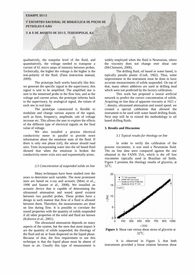
Figure 3 presents the rheology results of glycerin, at

320C.

Figure 3. Shear rate versus shear stress of glycerin at

320C.

It is observed in Figure 3, that both

instruments provided a linear relation between shear

ENAHPE 2013



rate and shear stress, classifying the glycerin is a

Newtonian fluid, as expected. The six points

represented by the stars are the six shear rates

provided by FANN 35A, and the high frequency

points are the ones provided by the on line instrument.

The vertical bars are the experimental uncertainties based on the accuracy of each sensor. Both

measurements agree statically. Table 2 provides the

values for the curve fitting of both data, using the

Newtonian model.

Table 2. Results for the Newtonian fit of glycerin, at

320 C.

Device µ (cP) R2

TT-100 16.3 ± 5.5.10-5 0.98

FANN 35A 15.8 ± 3.2.10-4 0.99

Results in Table 2 demonstrated that both

instruments provided statistically the same viscosity.

To test the performance of a Non-Newtonian

fluid, a CMC solution was prepared with a

concentration of 1% in mass. Figure 4 demonstrates

the results obtained.

Figure 4. Shear rate versus shear stress of a 1% CMC

solution at 330C.

Figure 4 presented a nonlinear relation

between shear rate and shear stress. The

characteristics of this curve classify the CMC solution

as a pseudo plastic fluid, as expected (Morrison,

2001). Observing the performance of both instruments, together with the degree of each error

bar, we conclude that some minimal divergences were

found. The possible main cause of these divergences is

the size of the gap of each instrument. The larger the

gap is the larger is the error due to numerical

approximation during the calculus of shear rate for

non-Newtonian fluids (Billon, 1996).

Table 3 presents the results for the curve fitting done over the data of Figure 4. Power law

model was used to fit the data.

Table 3. Results for the non-Newtonian fit of CMC

solution, at 330 C.

Device K n R2

TT-100 2.72 ±

9.97.10-3

0.46 ±

5.63.10-4 0.99

FANN 35A 3.24 ± 0.52 0.44 ±

2.46.10-2 0.99

In Table 3, K and n are the power law

experimental parameters.

It can be observed in this table that both the

behavior index (n) and the index of consistency (K)

are statically the same, although for the behavior index

the average value is more similar. Qualitatively, both

instruments provided the same intensity on the

nonlinearity of the relation between shear rate and

stress, but for TT-100, the fluid seems to be less

viscous that for FANN 35A.

To test drilling fluids, we prepared a water based mud in the drilling flow loop. We also used an

oil based mud, provided by an oil field company.

Figure 5 presents the results for the water based mud.

Figure 5. Shear rate versus shear stress of water based

mud at 340C.

ENAHPE 2013



It can be seen in Figure 5 that the shape of the

curves provided by both viscometers is not the same,

although the tendencies are as expected, pseudo

plastic. The probable causes for this divergence may

be pointed as the gap size effect associated with the

slippery effect. This last one is present when solids are suspended inside the gap. Slippery causes errors

during measurements because the velocity of the fluid

at the wall of the inner cylinder may fluctuate.

Especially with fluids that have lower lubricity, as

water based (Barnes, 2000). Table 4 presents the

values for the power law parameters.

Table 4. Results for the non-Newtonian fit of water

based mud, at 340 C.

Device K n R2

TT-100 1.85 ±

3.51.10-2

0.48 ±

2.90.10-3 0.99

FANN 35A 4.20 ±

8.91.10-2

0.37 ±

3.28.10-3 0.99

The disagreement on the curves found in

Figure 5 is found on the experimental parameters K

and n. They are not the same, not even statistically.

Figure 6 demonstrates the results obtained for

the rheology of oil based drilling fluid.

Figure 6. Shear rate versus shear stress of oil based

mud at 510C.

During the measurement of the oil based

fluid, it can be seen that after 500 s-1 the curve started to deviate from the off line one. Because the oil based

fluid has higher lubricity when compared to water

based fluids, the behavior during measurement found

in Figure 6 is the opposite found in Figure 5. In the

first TT-100 tends to underestimate the shear stress,

when compared to FANN measurements, in the last

one, it overestimates.

To evaluate the rheological model, we used the generalized power law model, also known as

Herschell-Buckley model. Table 5 shows the results of

the parameters.

Table 5. Results for the non-Newtonian fit of oil

based mud, at 510 C.

Device τ0 K n R2

TT-100 3.69 ±

0.07

0.07 ±

1.16.10-3

1.00 ±

2.44.10-3 0.99

FANN 35A

2.57 ± 0.44

0.17 ± 0.02

0.85 ± 0.02

0.99

The divergences found in the parameters in

Table 5 are a consequence of the divergence found in

the curves presented in Figure 6. Because the profile

provided by TT-100 is a very flatten curve, n is 1,

differently from FANN 35A, which is 0.85.

Usually drilling fluids have thixotropy

characteristics, useful to maintain the solids suspended

when the circulating process has stop, i.e., during the

connection of more drilling columns. Therefore, API

describes a methodology to characterize this coercion forces, known as jellification (Macosko, 1994). Many

on line experiences of jellification were done trying to

correlate the results with off line ones, but due to

geometrical and physical differences existent between

the viscometers, the comparison led to no conclusions.

One of the causes of these divergences may reside on

the difference of the spring constant of each

viscometer. The torsion element of TT-100 is

proximately 930 times greater than the spring constant

of FANN 35A.

To overcome this, we proposed another

methodology to evaluate the jellification. We created a virtual controller box that will make the viscometer

work as a rheometer. It creates a controlled ramp

upwards and downwards, with constant rate,

beginning in zero, passing through the desired

maximum shear rate and then returning to zero. If both

profiles do not superimpose each other, that means the

fluid has thixotropy characteristics. This methodology

is widely used on off line standard rheometers, and is

ENAHPE 2013



found in literature as the method of the hysteresis

(Schramm, 1995).

In order to test the virtual controller, we made

an experiment with a fluid that we know previously

that has no jellification. We used a mineral oil, a

Newtonian fluid. Figure 7 presents the results for the methodology.

Figure 7. Shear rate versus shear stress of mineral oil

during thixotropy at 270C.

After the test, the program automatically fit a

power law curve on the ascending and descending

data, and then calculates the area existent between

them. This allows the user to compare the parameters

of both curves and the size of the area. The more

similar the parameters are the less thixotropy is

detected; consequently the area tends to zero.

It is observed in Figure 7 that both profiles

are superimposed. This can be confirmed observing

the values of the parameters in Table 6.

Table 6. Results for the non-Newtonian fit of the

ascending and descending curves of mineral oil, at 270

C.

Curve K n Area

(Pa.s-1)

Ascending 0.076 1 20

Descending 0.078 0.99

The mineral oil has 76cP of viscosity during

ascending curve and 78cP during descending curve. The index behavior shows that the fluid is Newtonian,

n=1. The difference of both curves is inside the

experimental error and was considered similar. The

area between the curves is 20 Pa.s-1, which is not

considered a significant value; this value can achieve

more than 1000 Pa.s-1. Therefore, we validated our

virtual controller.

It is known that the xanthan gum (GX) is the substance responsible for the thixotropy characteristics

of water based fluids. Thus, Figure 8 demonstrates the

results obtained on water based mud.

Figure 8. Shear rate versus shear stress of water based

mud during thixotropy at 400C.

Observing both curves, it can be seen that the

fluid is more viscous during the ascending curve and

less viscous during the descending one. The viscosity

is the rate of shear stress by shear rate. In example, if

the shear rate of 5 s-1 is observed, one can draw a

vertical line of reference over the data, it will be

noticed that there are two different shear stresses

associated to the same value of shear rate. This characteristic is called hysteresis, and it is reversible

thermodynamically.

During the first few seconds of flow inside

the gap, the fluid molecules are changing geometry,

which is the main cause why the fluid is more viscous.

After a while, the molecules reach equilibrium

between flow forces and inner interaction forces,

staying in its final stage. For this type of fluids, the

shear stress not only depends on shear rate, but also on

time. Depending on time, means in another words, that

the jellification state of the fluid is a function of its

shear history. Because the fluid under measurement was constant being pumped, in every thixotropy test

the system had to be stop automatically. This would

ENAHPE 2013



allow the polymer to recover its folding state, gaining

viscosity over time. The time used of rest was the

same time suggest by the API test, 10 minutes. Only

after this time the viscometer started measuring.

To confirm numerically the hysteresis, Table

7 is presented with the curve fitting parameters. In this case it was used the generalized power law model,

with an extra parameter, due to an extra force needed

to put the fluid into motion.


ascending and descending curves of water based mud,

at 400 C.

Curve τ0 K n Area

(Pa.s-1)

Ascending 26.34 1.29 0.55 281

Descending 20.23 3.10 0.43

Observing the parameters and the calculated

area in Table 7, one may confirm the hysteresis

presented in Figure 8. Both curves presented distinct

coefficients and the area is more than ten times greater

than the area presented in Table 6.

Figure 9 presents the results for thixotropy

characterization of an oil drilling mud.

Figure 9. Shear rate versus shear stress of oil based

mud during thixotropy test at 400C.

Due to differences on the substance that

causes the thixotropy effect, TT-100 ascending curve,

demonstrated in Figure 9, presented a pick on the

shear stress when the system was immediately put into

motion. Probably the forces of coercion present in this

polymer are much more intense than the one existent

in xanthan gums.

The fit was not capable of predicting this

behavior, thus, for measurement purpose, this part of

the curve was not considered during the calculus. We

are implementing improvements in this sense to correct this issue.

There is hysteresis in Figure 9. The profiles

are not superimposed. Table 8 corroborates this

affirmative.


ascending and descending curves of oil based mud, at

290 C.

Curve τ0 K n Area

(Pa.s-1)

Ascending 4.83 0.11 0.99 242

Descending 2.29 0.19 0.90

Although we have done an approximation to

perform the calculus, the parameters are different

when Table 8 is observed and the area is sufficient

large to corroborate the hysteresis.

3.2 Typical results for density on line

The constant monitoring of density is imperative to maintain the drilling operations under

control, especially if overbalance technique is being

used (Craft, 1962). We compared the density acquired

on line against the results obtained in the off line mud

balance, instrument commonly used to measure

density of drilling fluids at rigs. Figure 10

demonstrates the first result, which was to monitor the

densification of a water based drilling fluid.

ENAHPE 2013



Figure 10. Density and temperature as a function of

time during the test of densification of water based

mud.

In Figure 10 each step upwards means that barite was added to the tank. The discontinued

horizontal points, in blue are the off line

measurements, as the high frequency ones the on line.

The other high frequency data is the temperature of

the test. The vertical bars are the experimental error (if

off line) or the device accurateness (if on line).

Isothermally we added known quantities of

barite to the tank and the device provided statistically

the same density as the off line one. After this

addition, we heat up the fluid to test if the on line

device was capable of correcting the density due an

increase on the temperature. Observing the temperature curve, referenced on the right vertical axis

of Figure 10, it can be seen a decrease on the density

as the temperature arises. Because the off line

instrument do not have temperature control, this

measurement was only done in the on line device.

The next experiment was done over the

previously dense fluid, but this time we made a

controlled dilution. We added quantities of water and

verified the new density after each step. There was a

point that the tank was at its maximum capacity,

therefore we purged it to allow more dilution. It can be seen in Figure 11 the black and blue data, they are the

on line and off line density respectively, the error bars

were omitted this time. The red data is the volume of

tank, referenced at the right axis.

Figure 11. Density and volume of the tank as a

function of time during the test of dilution of water

based mud.

It can be observed in Figure 11 that both on

line and off line data of density agrees statistically over a large range of density.

To verify the performance of the on line

device when oil fluid is used, we added barite to an

emulsion in the same methodology used in Figure 10.

Figure 12. Density and pressure of the pump as a

function of time during the test of densification of oil

based mud.

We could not dense more the oil mud

because the safe operational limit of pressure is

proximately 6 bars. The performance with oil based muds was similar to the one observed for water based

muds. This is an advantage because confers versatility

to the device.

ENAHPE 2013



3.3 Typical results for monitoring emulsion

state of oil based fluids on line

These tests are exclusively applied to oil

based muds. Although it receives this name, oil muds

are in fact an emulsion between oil and water. Depending on the chemistry of the emulsifier, it can

be obtained water in oil emulsions or oil in water

emulsion (Schramm, 2000).

An emulsion state is unstable

thermodynamically, therefore it is needed a third agent

to sustain such condition (Pal, 1993). Thus it is

necessary to monitor constantly its state. If an

emulsion is broken, the safety of the drilling process

will be compromised, because all physicochemical

properties rely on the emulsion condition, mostly

rheology (Fingas and Fieldhouse, 2003), which is

related directly to the pressure applied over the well (Craft, 1962).

API describes an electrical method to

quantify how stable is the emulsion and there is an off

line device constructed by FANN which performs

such measurements. We used our prototype to acquire

on line measurements of this stability and compared

against the ones provided by the off line instrument.

To evaluate our installation and calibration, we did

batch tests in a Becker using three different emulsion

samples with different rates of oil and water.

The first result was obtained in an emulsion of 50/50 (oil/water), demonstrated in Figure 13. In this

Figure, the voltage and amperage is demonstrated in

the left and right vertical axis, respectively. As the

voltage increases the current maintains its value at low

levels until it rapidly increases exponentially. At this

point, the electrical barrier provided by the oil phase is

broken and the polar part of the system, in this case

water, is exposed. This causes the electrical resistance

to low its value, and according to ohms law, the

current generated is direct proportional to the voltage

applied and inversely proportional to the electrical

resistance. Each fluid has its own voltage reference, which is the voltage peak when the current reaches 61

µA (Fann instruction manual, 2009).

Figure 13. Voltage and current in function of time

during electrical stability test, sample 50/50.

The voltage on line is represented by the

continuous line, the off line one by the continuous

blue horizontal one. The on line data is called EEON (Electrical Stability ON line) and off line is FANN.

The points are the on line electrical current monitored.

The voltage measurement is done synchronously to

the current measurements; we used a line to help

identify the voltage peak. The red dots at 61 µA mark

the current limit of the test, as specifies API. In this

case, the off line measurement of electrical stability

was around 800V. This value is in fact the average

value of several replicates, and the standard deviation

is showed by the vertical bars on top of the line. It can

be observed that the on line data (done in triplicate) is

slightly below the off line one, for this case 775V. The next sample is a 40/60 (oil/water) emulsion, the results

are presented in Figure 14.



ENAHPE 2013



As the ratio of water increases, the electrical

stability decreases, as expected. This can be observed

in Figure 14 when one compare the voltage peak

presented in this Figure with the one presented in

Figure 13. Qualitatively it is needed less energy to

brake the dielectric barrier, or in another words, it is needed a lower potential to achieve the current limit.

In this case the voltage peak for both

instruments is statistically the same.

The third batch experiment were done in an

emulsion of 30/70 (oil/water). Figure 15 presents the

results.



The peak voltage in Figure 15 is the smallest

one presented so far, due to the addition of more water

into the emulsion. The on line prototype presented

statistically the same results as the off line standard

one.

The last experiment done was to simulate a

real process condition. The system was submitted to

some controlled water invasion and controlled oil addiction. The state of the emulsion was monitored

only on line, and rheology was monitored as well.

After a while we submitted the system to an emulsion

breakage and observed the results. We will present in

the next Figures the operational conditions of the test.

Figure 16. Volume of the tank and density of the oil

mud during drilling simulation experiment.

Figure 17. Flow rate, pressure and temperature of the

oil mud during drilling simulation experiment.

Figure 18. Apparent viscosity profile of the oil mud

during drilling simulation experiment.

ENAHPE 2013



Starting with the oil at its original

characteristics of density, rheology and emulsion state,

we added controlled portions of pure oil. This addition

caused the volume of the tank to rise up and

consequently the original value of density started to

decrease. Reaching the capacity of the tank, it was done a purge, decreasing its volume to a minimum

required for continuing the pumping process. At this

stage, we started to add water, until the tank is full

again. We kept purging it to the minimum level and

fulfilling it with water again. We repeated it until the

emulsion was broken. This process is demonstrated in

Figure 16.

Figure 17 shows the pressure, flow rate and

temperature of the whole system. The constant drop to

zero on pressure and flow rate is due to the stop of the

pump every time an electrical stability test was

performed. It is known that this test must be done at static system, as API describes. Relative velocity

between the probe and sample may cause different

results (Saasen, 2009).

Still in Figure 17, it can be seen that flow rate

was kept at a minimum level in order to maintain a

renewal of the fluid inside the electrical stability and

conductivity measuring chamber, when the electrical

stability test was not active. When oil was being

added, it decreased the apparent viscosity and density,

causing the pressure to also decrease. When water was

being added, although the density still kept decreasing, there was a significant increase on the apparent

viscosity, causing the pressure to rise. At the end of

the test, when the emulsion was broken, there was an

abrupt decrease on the apparent viscosity, which

caused a decrease on pressure. Also in this Figure is

demonstrated the temperature profile of the test. It is

possible to see that every time a perturbation was done

the system was cooled, as it recovers the steady state,

it started to warm up again. The heat exchanger was

not used; the heating was caused exclusively by

friction between the hydraulic parts and the fluid.

The behavior of the apparent viscosity can be seen in Figure 18. Because the viscometer acquires the

rheological profile, the viscosity demonstrated in this

Figure is also a profile, due to the non-Newtonian

behavior of the fluid. Observing Figure 18 we see in

the first measurement the original viscosity profile of

the oil mud. From the second one, oil was already

added to the system, one can note that the second

profile has lower values of viscosity, in general. From

instant 4000s to 7000s the constant addiction of oil did

not change considerably the rheology of the fluid, but

from 7000s, when water started to be added, the

apparent viscosity started to increase exponentially.

The increase reaches its maximum point at 12000s,

proximately, and from there an abrupt decrease is

observed. At this stage the emulsion was broken. Figure 19 shows the general electrical

monitoration of the emulsion state during the

described test.

Figure 19. General electrical behaviour of the oil mud

during drilling simulation experiment.

The olive lines are the voltage picks as the

black ones are the current picks. The blue dots are the

on line data of electrical conductivity.

According to Figure 16, we added oil until

proximately 6000s. Observing Figure 19 we

understand that oil alone does not change the electrical

stability of the system significantly, but the addition of

water after that immediately starts to decrease the voltage picks. As water went into the system, the

voltage picks kept decreasing. It was observed in all

Figures that proximately at 12000s the system

changed its state drastically due to the breakage of the

emulsion; this is confirmed looking at the same

moment in Figure 19. Not only the voltage picks are

less than 25V but the electrical conductivity deviates

from 0. When the emulsion was stable, the

conductivity meter marked 0.

Therefore, the electrical stability meter is a

tool that can indicates the state of the emulsion while

there is one phase only, and the conductivity meter can be used as an auxiliary tool that detects the

breakage of it (phase separation).

ENAHPE 2013



3.4 Typical results for monitoring suspended

solids

This work used an ultrasonic sensor to

calculate such measurement. It is not possible to

calculate this variable directly from measurements of volume and density, at least not in real time. But only

the ultrasonic sensor is not sufficed to determine the

concentration of the solids suspended in drilling muds.

This is because drilling fluids are more complex in

rheology. Ultrasonic attenuation and sound speed

depend not only on the quantity of the solids

suspended, but also on the quantity of solids

dissolved, like salts and mainly on rheology.

Therefore, to determine the total solids suspended it

was acquired not only the ultrasound attenuation and

sound speed, but also apparent viscosity at 1021 s-1

and density. We classified, for better understanding, the measurements of ultrasound attenuation and sound

speed as main variables and the measurement of

density and apparent viscosity as auxiliary ones. These

auxiliary measurements help the software made to

discern when an increase of attenuation is due to the

increase of viscosity or solids. In example, if an

increase on attenuation is due to the entrance of solids

into the system the density should also increase, and

maybe some increase may be observed on viscosity. In

other hand, if an increase on the attenuation is

observed due addition of polymers (viscosity agent), the density may change slightly or not even change.

The sound speed is also important because it helps the

system to discern when the density is rising due to

solids suspended or solids dissolved. In example,

some water drilling fluids have high densities not only

due to the solids suspended, like barite, but also for

large amounts of salt dissolved.

The mentioned software is capable of

receiving these four measurements and calculating the

concentration of solids suspended. The mathematical

methodology to relate those variables was based on an

artificial neural network, trained from the cumulated experimental results over the past few years.

The experiments were done during the

production of many different types of water based

muds and also from simulations of disturbances.

To validate the on line results of

concentration, samples were taken during the tests and

using gravimetric technique, the off line concentration

was determined. During the network training,

concentration of the suspended solids was the target

variable, and density, viscosity, ultrasound attenuation

and sound speed were the independent variables. The

next Figures are a demonstration of the some

experiments that were done to train the artificial

neural network.

Figure 20. Experimental concentration of solids

suspended, density, viscosity, ultrasound attenuation

and sound speed during making water based mud 1.

It can be seen in Figure 20 that we started the

system without solids, just industrial water. Initial

configurations of the other variables were at its stages: viscosity was about 2 cP at 1021 s-1, density was about

1,00 kg/l, the sound speed was 1495 m/s and

attenuation was proximately 5,5 dB. When the first

kind of solid was added to the system, the

concentration raised to proximately 60 g/l (off line

measurement), the attenuation raised to 8 dB, the

apparent viscosity raised to 5,5 cP, density was up to

1,02 kg/l and sound speed decreased to 1490 m/s.

When we added the second kind of solid the system

changes all its stage again. In this manner, the

software started to “learn” how the system behaves. The empty spaces between the measurements are the

transient stages, and does not interest to the network

training because the experimental concentration of

solids in this period is unknown. Figure 21

demonstrates the fabrication of a second type of water

drilling fluid.

ENAHPE 2013



Figure 21. Experimental concentration of solids

suspended, density, viscosity, ultrasound attenuation


In this fluid we also started from industrial

water, but this time we added at first a polymer to

increase viscosity. Due to the very small quantities

applied (less than 1%), density practically doesn’t change, only viscosity. It can be seen in Figure 21 that

the solids were zero in the beginning and is still zero

during the dissolution of the polymer, as it should be.

It can also be observed that after the polymer is

dissolved the viscosity increased significantly, as the

density practically didn’t change. The attenuation

increased from 5 to 10 dB. Because the polymer goes

to the dissolved phase, the sound speed also changes

significantly. After 7000s we added the solids, the

system reacts accordingly.

We shall demonstrate one result obtained

during the simulation of operational disturbances, such as solid invasion, in the next Figures.

Figure 22. Experimental concentration of solids suspended, density, viscosity, ultrasound attenuation


In Figure 22 the initial state was a water

drilling fluid with low concentration of solids

suspended. We added a solid of kind A to the fluid

simulating an invasion into the fluid. This increased

all the properties except for the sound speed, which

decreased. Next step we added a solid of kind B to the system, this solid is heavy, it increased significantly

the density and slightly the viscosity. The sound speed

kept decreasing as attenuation and concentration

increased. In the final two steps we simulated an

invasion of carbonate rocks. The system kept the same

tendency except for the sound speed, which started to

increase instead of decreasing. All those results in

addition with much more data were used to train the

neural network. Figure demonstrates the general

performance of the prediction capacity of the

architecture made.

Figure 23. Concentration of solids suspended

predicted by the artificial neural network (Output)

against experimental one (Target).

Figure 23 presents the comparison between

the concentrations of solid predicted by the network,

named “Output”, and the ones determined

experimentally, named “Target”. In this kind of

graphic, if the points are superimposed on the 45

degree line, it means x=y. Therefore, the closest the

points are to the line the best was the performance of

the network. Of all the points presented in Figure 23,

80% were used during training and 20% were used for

validation. Validation points are not used during training and their performance indicates the predictive

capacity of the network. To accomplish such

performance we used MLP architecture, 50 neurons,

ENAHPE 2013



exponential function in the inner layer and identity

function in the outer layer.

This methodology will be extended to oil

drilling muds in future.

4. Conclusion

This work has built an automation drilling

flow loop not only do make drilling fluids but also to

test and develop drilling fluid sensors. We

demonstrated results of rheology, density, electrical

stability and electrical conductivity and concentration

of solids measured in real time. We acquired sensors

from vendors, some were modified, methodologies

were proposed and one sensor was totally developed.

The results has shown that is possible to measure the

properties on line based on the agreement found

between the on line data and off line one, in most cases. Although much effort is found in literature

focusing on automation of the drilling fluid

physicochemical properties, their complexities and the

harsh oil field scenarios are still challenges for today’s

technologies.

5. References

CRAFT, Holden and Graves, 1962. Well Design:

Drilling and Production. Prentice – Hall, Inc. Englewood Cliffs, New Jersey.

LUYBEN, W. L., 1996. Process Modeling,

Simulation, and Control for Chemical Engineers.

McGraw-Hill, Inc. Lehigh University, US.

SAASEN, A., OMLAND, T. H., EKRENE, S.,

BRÉVIÈRE, J., VILLARD, E., KAAGESON-LOE,

N., TEHRANI, A., CAMERON, J., FREEMAN, M.,

GROWCOCK, F., PATRICK, A., STOCK, T.,

JØRGENSEN, T., REINHOLT, F., AMUNDSEN, H.

E. F., STEELE, A., MEETEN, G., 2009. “Automatic Measurement of Drilling Fluid and Drill-Cuttings

Properties”. SPE/IADC Drilling Conference and

Exhibition, Orlando, Florida. SPE 112687.

BROUSSARD, S., GONZALEZ, P., MURPHY, R.,

MARVEL, C., 2010. “Making Real-Time Fluid

Decision with Real-Time Fluid Data at the Rig Site”.

Society of Petroleum Engineering (SPE). SPE

Drilling Conference and Exhibition, Abu Dhabi, UAE.

SPE 137999.

MILLER, A., MINTON, R. C., COLQUHOUN, R.,

KETCHION, M., 2011. “The Continuous

Measurement and Recording of drilling Fluid Density and Viscosity. SPE/IADC Drilling Conference and

Exhibition, Amsterdam, The Netherlands. SPE/IADC

140324.

MOTZ, E., CANNY, D., EVANS E., BAKER

HUGHES INTEQ., 1998. “Ultrasonic Velocity and

Attenuation Measurements in High Density Drilling

Muds”. Society of Petrophysicists and Well-Log

Analysts. ID 1998-F, Conference Paper.

KOLTZOVA, I. S., MUKEL M., DYATLOVA E. N.,

2001. “Velocity and Attenuation of Ultrasonic Waves in Suspensions”. XI Session of the Russian Acoustical

Society. Moscow, Russia. Institute of Physics, St-

Petersburg State University.

FANN INSTRUMENTS, revision C, Part No. 209064,

Model 23D Electrical Stability Tester, Instruction

Manual.

BROOKFIELD INC., 1993. Instruction Manuals and

Guides.

McCLEMENTS, D. J., 2006. Ultrasonic

Measurements in Particle Size Analysis. Encyclopedia

of Analytical Chemistry, ISBN 0471 97670 9.

BARNES, H. A., 2000. A Handbook of Elementary

Rheology. Institute of Non-Newtonian Fluid

Mechanics, University of Wales.

BILLON, H.H., 1996. “Shear Rate Determination in a

Concentric Cylinder Viscometer”. DSTO Aeronautical

and Maritime Research Laboratory, Melbourne.

Publication track AR-009-701, DSTO-GD-0093.

MORRISON, F. A., 2001. Understanding Rheology,

Oxford University Press, Inc. ISBN 0-19-514166-0.

MACOSKO, C. W., 1994. Rheology: Principles,

Measurement and Applications. Wiley-VCH – Inc. Originally publish as ISBN 1-56081-579-5.

ENAHPE 2013



SCHRAMM, G., 1995. A Practical Approach to

Rheology und Rheometry. Thermo Haake GmbH,

Karlsruhe.

PAL, R., 1993. “Techniques for Measuring the

Conposition (Oil and Water Content) of Emulsions – a State of the Art Review”. Colloids and Surface A:

Physicochemical and Engineering Aspects, 84 (1994)

141-193, Elsevier Science B.V. Department of

Chemical Engineering, University of Waterloo,

Canada.

FINGAS, M., FIELDHOUSE, B., 2003. “Studies of

the Formation Process of Water-in-Oil Emulsions”.

Marine Pollution Bulletin 47 (2003) 369-396.

Emergencies Science and Technology Division,

Environment Technology Centre, Canada.

SCHRAMM, L. L., 2000. Surfactants: Fundamentals

and Applications in the Petroleum Industry.

Cambrigde University Press, Cambridge, 2000.

enahpe 2013 v encontro nacional de hidráulica de poços de...

Documents