remote sensing

Article

Emulation of Leaf, Canopy and Atmosphere RadiativeTransfer Models for Fast Global Sensitivity Analysis

Jochem Verrelst 1,*, Neus Sabater 1, Juan Pablo Rivera 1,2, Jordi Muñoz-Marí 1, Jorge Vicent 1,Gustau Camps-Valls 1 and José Moreno 1

1 Image Processing Laboratory (IPL), Parc Científic, Universitat de València, Paterna 46980, Spain;m.neus.sabater@uv.es (N.S.); rijuanpa@uv.es (J.P.R.); jordi.munoz@uv.es (J.M.-M.); jorge.vicent@uv.es (J.V.);Gustau.Camps@uv.es (G.C.-V.); jose.moreno@uv.es (J.M.)

2 Departamento de Oceanografía Física, Centro de Investigación Científica y de Educación Superior deEnsenada, Ensenada 22860, Mexico

* Correspondence: jochem.verrelst@uv.es; Tel.: +34-96-354-4067; Fax: +34-96-354-3261

Academic Editors: Lenio Soares Galvao, Clement Atzberger and Prasad S. ThenkabailReceived: 9 April 2016; Accepted: 16 August 2016; Published: 19 August 2016

Abstract: Physically-based radiative transfer models (RTMs) help understand the interactions ofradiation with vegetation and atmosphere. However, advanced RTMs can be computationallyburdensome, which makes them impractical in many real applications, especially when many stateconditions and model couplings need to be studied. To overcome this problem, it is proposed tosubstitute RTMs through surrogate meta-models also named emulators. Emulators approximatethe functioning of RTMs through statistical learning regression methods, and can open manynew applications because of their computational efficiency and outstanding accuracy. Emulatorsallow fast global sensitivity analysis (GSA) studies on advanced, computationally expensive RTMs.As a proof-of-concept, three machine learning regression algorithms (MLRAs) were tested to functionas emulators for the leaf RTM PROSPECT-4, the canopy RTM PROSAIL, and the computationallyexpensive atmospheric RTM MODTRAN5. Selected MLRAs were: kernel ridge regression (KRR),neural networks (NN) and Gaussian processes regression (GPR). For each RTM, 500 simulationswere generated for training and validation. The majority of MLRAs were excellently validated tofunction as emulators with relative errors well below 0.2%. The emulators were then put into a GSAscheme and compared against GSA results as generated by original PROSPECT-4 and PROSAILruns. NN and GPR emulators delivered identical GSA results, while processing speed compared tothe original RTMs doubled for PROSPECT-4 and tripled for PROSAIL. Having the emulator-GSAconcept successfully tested, for six MODTRAN5 atmospheric transfer functions (outputs), i.e.,direct and diffuse at-surface solar irradiance (Edi f , Edir), direct and diffuse upward transmittance(Tdir, Tdi f ), spherical albedo (S) and path radiance (L0), the most accurate MLRA’s were subsequentlyapplied as emulator into the GSA scheme. The sensitivity analysis along the 400–2500 nm spectralrange took no more than a few minutes on a contemporary computer—in comparison, the sameanalysis in the original MODTRAN5 would have taken over a month. Key atmospheric driverswere identified, which are on the one hand aerosol optical properties, i.e., aerosol optical thickness(AOT), Angstrom coefficient (AMS) and scattering asymmetry variable (G), mostly driving diffuseatmospheric components, Edi f and Tdi f ; and those affected by atmospheric scattering, L0 and S.On the other hand, as expected, AOT, AMS and columnar water vapor (CWV) in the absorptionregions mostly drive Edir and Tdir atmospheric functions. The presented emulation schemes showedvery promising results in replacing costly RTMs, and we think they can contribute to the adoption ofmachine learning techniques in remote sensing and environmental applications.

Remote Sens. 2016, 8, 673; doi:10.3390/rs8080673 www.mdpi.com/journal/remotesensing

Remote Sens. 2016, 8, 673 2 of 27

Keywords: emulator; global sensitivity analysis; machine learning; radiative transfer models;PROSPECT; SAIL; MODTRAN

1. Introduction

Since the advent of optical remote sensing, physically-based radiative transfer models (RTMs)have deeply helped in understanding the radiation processes occurring on the Earth’s surface andtheir interactions with vegetation and atmosphere (e.g., [1,2]). RTMs are deterministic models thatdescribe absorption and scattering, and some of them even describe the microwave region, thermalemission or sun-induced chlorophyll fluorescence emitted by vegetation (e.g., [3,4]). They are usefulin a wide range of applications including (i) sensitivity analysis; (ii) developing inversion modelsto accurately retrieve atmospheric and vegetation properties from remotely sensed data (see [5] fora review); and (iii) to generate artificial scenes as would be observed by an optical sensor (e.g., [6,7]).Plant and atmospheric RTMs are currently used in an end-to-end simulator that functions as a virtuallaboratory in the development of next-generation optical missions [8,9].

When it comes to vegetation analysis, RTMs have found a wide range of applications to model,study and understand light interception by plant canopies and the interpretation of vegetationreflectance in terms of biophysical characteristics [2,10,11]. A diversity of canopy RTMs have beendeveloped over the last three decades with varying degrees of complexity. Gradual improvementin RTMs accuracy, yet in complexity too, have diversified RTMs from simple turbid mediumRTMs towards advanced Monte Carlo RTMs that allow for explicit 3D representations of complexcanopy architectures (e.g., see the RAMI exercises [12,13] for a meticulous comparison). Thisevolution has resulted in an increase in the computational requirements to run the model, whichbears implications towards practical applications. In general, RTMs can be categorized as either(1) ’economically invertible’ (or computationally cheap); or as (2) ’non-economically invertible’ models(or computationally expensive). These terms refer to the model complexity and associated processingspeed constraining the inversion of such models: Economically invertible models are models withrelatively few input parameters and fast processing that enables fast calculations and so applicationssuch as model inversion or rendering of simulated scenes. Examples of this category include thewidely used leaf RTM PROSPECT [14], canopy RTM SAIL [15] and atmospheric RTM 6S [16] andOSS [17].

Non-economically invertible RTMs refer to advanced RTMs, often with a large number of inputvariables and sophisticated computational and mathematical modelling. These type of RTMs enablethe generation of complex or detailed scenes, but at the expense of a tedious computational load.In short, the following families of RTMs can be considered as non-economically invertible: (1) MonteCarlo ray tracing models (e.g., Raytran [18], FLIGHT [19] and Drat [20]); (2) voxel-based models(e.g., DART [21]) and (3) advanced integrated vegetation and atmospheric transfer models (e.g.,SimSphere [22], SCOPE [23] and MODTRAN [24]). Although these advanced models serve perfectlyas virtual laboratories for fundamental research on light-vegetation and atmosphere interactions (seee.g., [18,25]), their high computational cost make them impractical for applications such as inversion.Consequently, when it comes to selecting an RTM for applications that demand many simulations,the current pragmatic approach is to search for a good balance between acceptable accuracy andcomputational complexity [5].

Regardless whether an RTM is computationally expensive or not, an important requirement is theidentification of the key input variables driving the spectral output and variables of lesser influence.By identifying variables of lesser influence, models can be greatly simplified, which facilitates practicalapplications such as inversion [26]. To achieve this, a sensitivity analysis is required. A sensitivityanalysis can be simply defined as the process of determining the effect of changing the value of one ormore input variables, and observing the effect that this has on the considered model’s output [22,27].

Remote Sens. 2016, 8, 673 3 of 27

In general, sensitivity analysis methods can be categorized as either ‘local’ or ‘global’.Local sensitivity analysis (LSA) methods are often referred to as “one-factor-at-a-time”, becausethey involve changing one input variable at a time whilst holding all others at their default values,then measuring variation in the outputs. A drawback of LSA methods is that they are informative onlyat the default point where the calculation is executed and do not encompass the entire input variablespace. Thus, LSA methods are inadequate for analysis of complex models having many variables, andthat may be highly dimensional and/or non-linear [27–29]. Unlike LSA, global sensitivity analysis(GSA) explores the full input variable space [27]. Variance-based GSA methods aim to quantify theamount of variance that each input variable contributes to the unconditional variance (variance acrossall simulations) of the model’s output [29]. The approach is able to quantify the sensitivity to eachof the model variables and their interactions, which cannot be done using LSA studies. GSA is thusrequired to identify the driving variables of an RTM. However, a GSA requires many simulations(depending on the number of variables, typically in the orders of 10 thousands), which makes itcomputationally demanding. It bears the consequence that so far GSA studies have been restrictedto merely abstract, computationally cheap models, typically coming from the PROSPECT and SAILfamilies (e.g., [30–33]).

Identification and quantification of key variables in realistic vegetation an atmospheric radiativetransfer interactions would enable a more sound understanding of atmospheric mechanisms withpractical applications towards improved retrieval schemes. In order to bypass the computationalburden of costly RTMs, in this paper a computationally effective technique is proposed by onlyusing a limited number of computer code runs. The technique consists of approximating the RTMby a surrogate model with low computation time, also referred to as meta-model or emulator [34].Once having a successful emulator developed, the idea is that it can replace the original RTM and bereadily applied to perform sensitivity analysis. Accordingly, we posit here that emulators can providean efficient mean for doing a GSA on large and expensive models.

Although successfully applied into GSA schemes for quantifying drivers of climate andenvironmental process-based models (e.g., [22,35,36]), so far this technique is largely unknown inremote sensing science. Only recently Rivera et al. (2015) [37] and Gómez-Dans et al. (2016) [38] startedexploring the possibility of emulating RTMs and applying them for retrieval applications. The authorsconstructed RTM-like emulators with capabilities to deliver accurately and quasi-instantly spectraloutputs such as reflectance, fluorescence and radiance. Advancing along this line, when emulatorsappear to approximate RTMs with high accuracy, consequently, it would become possible to applyGSA to any RTM, including computationally expensive RTMs such as MODTRAN.

In light of the above, the main objective of this study is to analyze the possibility of approximatingthe functioning of RTMs by emulators, in order implement these emulators into a GSA scheme forenabling analyzing computationally intensive RTMs into its driving input variables. This objective canbe broken down into the following sub-objectives: (1) to analyze three machine learning regressionalgorithms on their accuracy to function as emulators for three RTMs with increasing complexity at theleaf, canopy and atmosphere scale, i.e., PROSPECT-4, PROSAIL and eventually the computationallyexpensive RTM MODTRAN5; (2) to apply the PROSPECT-4 and PROSAIL-like emulators into a GSAscheme and compare its results against GSA reference results as obtained from original PROSPECT-4and PROSAIL simulations; and finally (3) to apply MODTRAN5-generated emulators for variousMODTRAN5 outputs into the GSA scheme to enable identifying driving atmospheric variables alongthe 400–2500 nm spectral range.

2. Emulator Theory

Emulation is a technique used to estimate model simulations when the computer model underinvestigation is too computationally costly to be run enough times [34]. Various emulators basedon statistical learning have already been developed in the climate and environmental modelingcommunity for the last few years (e.g., [22,35,36,39–43]). These emulators have in common that they

Remote Sens. 2016, 8, 673 4 of 27

were developed from adaptive, flexible nonparametric regression algorithms, typically within thefamily of machine learning regression algorithms (MLRAs) [44]. Examples of MLRAs include Gaussianprocesses regression and neural networks [38,45]. The emulator uses a limited number of simulatorruns, i.e., input-output pairs (corresponding to training samples), to infer the values of the complexsimulator output given a yet-unseen input configuration. With respect to applying emulators intosensitivity analysis, specific advantages of the emulator are [22]:

1. The emulator is derived from a relatively small number of model runs covering a multidimensionalinput space, and is used to derive a computationally inexpensive and efficient analysis of all thesensitivity analysis computations regarding the original deterministic model code.

2. Once the emulator is built, it is not necessary to perform any additional runs with the model,regardless of how many analyses are required to assess the simulator’s behaviour. This is a veryimportant advantage in the use of this method compared to other conventional GSA methods(e.g., those reviewed in [27] that typically require a fresh set of simulator runs for each analysis).Therefore, compared for instance to Monte Carlo-type methods, the approach requires far fewermodel runs since the original code is only run to build the dataset to train the emulator.

Consequently, a two-step approach is pursued. The first step involves building a statistically-basedrepresentation (i.e., an emulator) of the simulator (i.e., an RTM) from a set of training data pointsderived from runs of the actual model under study. These training data pairs should ideally cover themultidimensional input space using a space-filling algorithm. Only one set of runs of the simulator isused to build the emulator. After the emulator is built, no more simulator runs are needed, no matterhow many analyses are required of the simulator’s behavior. The second step uses the emulator builtin the first step to compute the output that is otherwise generated by the simulator [34]. Note thatbuilding an emulator is essentially the same as building nonparametric regression models used forretrieval (e.g., [46,47]), but then in reversed order: whereas a retrieval model converts reflectance inputinto one or more output biophysical variables, an emulator converts input biophysical variables intooutput spectral data.

An important criterion regarding emulating an RTM is the ability to deliver a full spectrum, i.e.,spectral output at multiple bands. This bears the consequence that the MLRA (i.e., emulator) shouldbe able to generate multiple outputs in order to reconstruct a full spectral profile. However, the full,contiguous spectral profile typically consists above 2000 bands when binned to 1 nm resolution.This can take considerable training time, especially when using neural networks [37]. To enablethe models to cope with large hyperspectral datasets (e.g., reflectance, transmittance, fluorescence),applying a principal component analysis (PCA) dimensionality reduction step [48] prior to training amodel has been implemented. This step consists on projecting the RTM output spectra onto the topeigenvectors computed with PCA, p B, where p is the number of selected components (usuallyone typically takes enough components to ensure that at least 99.9% of variance is retained), and B isthe number of original bands of the spectra. The regression methods are then trained to predict thePCA reduced spectra, and the inverse of the PCA transformation is subsequently applied to obtainthe reconstructed output spectra. This dimensionality reduction strategy not only greatly speeds upthe training phase but also makes the problem better conditioned [36–38]. An additional advantageof applying the PCA transformation is that it allows converting single-output MLRAs into multipleoutput methods, i.e., meaning that in principle any multivariate regression algorithm can functionas emulator. By first applying a PCA to spectral data the hyperspectral data is reduced to a givennumber of components. By subsequently looping over the single component multiple models canbe trained by a single-output MLRA. Afterwards the signal is again reconstructed. Although theiterative training takes some computational time, it is considerably faster than training a hyperspectraldataset band-by-band.

Based on the literature review above and an earlier comparison study conducted [37], the followingthree MLRAs potentially serve as powerful methods to function as emulators, being kernel ridgeregression (KRR), neural networks (NN) and Gaussian processes regression (GPR). These methods

Remote Sens. 2016, 8, 673 5 of 27

have been amply described in earlier publications (e.g., [5,38,44,46,49,50]). The interested readercan find more details therein. The source codes of each of these methods, along with many otheralternatives, are freely available in the simpleR toolbox [51]. The Automated Radiative Transfer ModelsOperator (ARTMO) Graphic User Interface (GUI) is a modular software package that includes theseMLRA methods as well [47], and as described later, provides some easy-to-use tools for running RTMsand further processing.

3. Global Sensitivity Analysis Theory

Various variance-based GSA methods have been presented in the literature, including the Sobol’method [52], the Fourier Amplitude Sensitivity Test (FAST) [53] and a modified version of the Sobol’method proposed by [54]. This modification has been demonstrated to be effective in identifying theso-called Sobol’s sensitivity indices. These indices quantify both the main sensitivity effects (first-ordereffects: Si, i.e., the contribution to the variance of the model output by each input variables) and totalsensitivity effects (STi, i.e., the first-order effect plus interactions with other input variables) of inputvariables. This method has been applied here. A description according to Song et al. (2012) [55] isgiven below.

Formally, we have a model y = f (x), where y is the model output, and x = [x1, x2, ..., xk]> is the

input feature vector. A variance decomposition of f (·) as suggested by Sobol [52] is:

V(y) =k

∑i=1

Vi +k

∑i=1

k

∑j=i+1

Vij... + V1,...,k, (1)

where x is rescaled to a k-dimensional unit hypercube Ωk, Ωk = x|0 ≤ xi ≤ 1, i = 1, . . . , k; V(y) isthe total unconditional variance; Vi is the partial variance or ‘main effect’ of xi on y and given bythe variance of the conditional expectation Vi = V[E(y|xi)]; Vij is the joint impact of xi and xj on thetotal variance minus their first-order effects. Here, the first-order sensitivity index Si and total effectsensitivity index STi are given as [27]:

Si =Vi

V(y) =V[E(y|xi)]

V(y) (2)

STi = Si + ∑j 6=i

Sij + ... =E[V(y|x∼i)]

V(y) , (3)

where x∼i denotes variation in all input variables and xi, Sij is the contribution to the total varianceby the interactions between variables. Following Saltelli et al. (2010) [54], to compute Si and STitwo independent input variable sampling matrices P and Q of dimensions N × k are created, where Nis the sample size and k is the number of input variables. Each row in matrices P and Q representsa possible value of x. The variable ranges in the matrices are scaled between 0 and 1. The Monte Carloapproximations for V(y), Si and STi are defined as follows [29,54]:

V(y) = 1N

N

∑j=1

( f (P)j)2 − f 2

0 , f0 =1N

N

∑j=1

f (P)j, (4)

and

Si =1N

N

∑j=1

f (Q)j( f (P(i)Q )j − f (P)j)

V(y), STi =

12N

N

∑j=1

( f (P)j − f (P(i)Q )j)

2

V(y), (5)

Remote Sens. 2016, 8, 673 6 of 27

where . . . is the estimate; f0 is the estimated value of the model’s output; we abused notation bydefining f (P) as all outputs for row vectors in P; P(i)

Q represents all columns from P except thei-th column which is from Q, using a radial sampling scheme [56]. Matrices are generated witha Latin hypercube sampling of size N × 2k where P and Q are the left and right half of this matrix,respectively [54]. In order to compute Si and STi simultaneously, a scheme suggested by [57] was usedwhich reduced the model runs to N(k + 2).

4. Applied RTMs

As a proof-of-concept, the utility of emulators into the GSA framework will be demonstrated forthree different RTMs at three scales with increasing degree of complexity, i.e., PROSPECT-4 at the leaf,PROSAIL at the canopy, and MODTRAN5 at the atmospheric scale. A brief description of the selectedRTMs is given below.

4.1. PROSPECT-4

At the leaf scale, the PROSPECT-4 model [14] is currently one of the most widely used leafoptical models and is based on earlier PROSPECT versions. The model calculates leaf reflectance andtransmittance as a function of its biochemistry and anatomical structure. It consists of four parameters,those being leaf structure (N), equivalent water thickness (Cw), chlorophyll content (Cab) and drymatter content (Cd). PROSPECT-4 simulates directional reflectance and transmittance over the solarspectrum from 400 to 2500 nm at the fine spectral resolution of 1 nm.

4.2. PROSAIL

At the canopy scale, SAIL is the most popular canopy RTM; also likely due to its availabilityand rather low number of input variables [15]. SAIL is based on a four-stream approximation ofthe RT equation, in which case one distinguishes two direct fluxes (incident solar flux and radiancein the viewing direction) and two diffuse fluxes (upward and downward hemispherical flux) [58].SAIL inputs consist of leaf area index (LAI), leaf angle distribution (LAD), ratio of diffuse and directradiation (skyl), soil coefficient (soil coeff.), hot spot and sun-target-sensor geometry, i.e., solar/viewzenith angle and relative azimuth angle (SZA, VZA and RAA, respectively). Spectral input consists ofleaf reflectance and transmittance spectra and a soil reflectance spectrum. The leaf optical propertiescan come from a leaf RTM such as PROSPECT. By coupling PROSPECT with SAIL (PROSAIL),a leaf-canopy model is generated that allows analyzing the impact of leaf biochemical variables at thecanopy scale [2]. PROSAIL generates hemispherical and bidirectional top-of-canopy (TOC) reflectanceas output.

4.3. MODTRAN5

At the atmosphere scale, MODTRAN5 [24], the moderate resolution transmittance code,is one of the most widely used radiative transfer codes in the atmospheric community [59].MODTRAN solves the radiative transfer equation by including the effects of molecular and particulateabsorption/emission and scattering, surface reflections and emission, solar/lunar illumination,and spherical refraction. The absorption and scattering processes, considering the atmosphericextinction both for aerosols and molecules, are rigorously calculated using DISORT [60] andCorrelated-k [61] algorithms. In addition, MODTRAN uses a spherically symmetric atmosphere,consisting of homogeneous layers, each one characterized by its temperature, pressure andconcentration of atmospheric compounds. Here, the Snell’s law is used to calculate the curvature oflight beams due to refraction between each atmospheric layer.

The large number of MODTRAN inputs (see [62] for a detailed description) allows the userto define the spectral range, illumination/viewing geometry and atmospheric state. A smallersubset of key input variables for general-purpose applications [63] (see Table 1) describe the main

Remote Sens. 2016, 8, 673 7 of 27

interactions between atmosphere and solar radiation in all spectral range. With respect to the geometricconditions, the key variables are SZA, VZA and RAA. Regarding the atmospheric state, the key inputvariables are reduced to two subsets: (1) Aerosol optical properties, described by means of theAerosol Optical Thickness (AOT), the Angstrom parameter (AMS), and the asymmetry parameterof the Henyey-Greenstein scattering phase function (G); and (2) total columnar water vapor (CWV).In addition, the surface pressure, determined by the topographic elevation (ELEV), completes the set ofkey inputs variables. Depending on the application, other variables (e.g., vertical temperature profile,vertical aerosol distribution, concentration of CO2) might be added. In our study, these variables areset to their default values.

Table 1. Range and distribution of input variables used to establish the PROSPECT-4, PROSAIL(PROSPECT4 + SAIL) and MODTRAN5 look-up tables. SAIL hot spot variable was fixed to 0.01.

Model Variales Units Minimum Maximum

Leaf variables: PROSPECT-4N Leaf structure index unitless 1.0 4.0Cw Leaf water content cm 0.001 0.05LCC Leaf chlorophyll content µg/cm2 0.1 100Cm Leaf dry matter content g/cm2 0.001 0.05Canopy variables: SAILLAI Leaf area index m2/m2 0.1 10LAD Average leaf angle 0 90skyl Diffuse incoming solar radiation fraction 0 100Soil coe f f . Soil scaling factor unitless 0 1SZA Sun zenith angle 0 60VZA View zenith angle 0 55RAA (Sun-sensor) relative azimuth angle 0 180Atmospheric variables: MODTRAN5VZA Visual zenith angle 0 55SZA Solar zenith angle 0 60RAA Relative azimuth angle 0 180ELEV Elevation km 0 2AOT Aerosol optical thickness - 0 0.4AMS Angstrom Coefficient - 0.5 3G Asymmetry parameter - −1 1CWV Columnar water vapor g/cm2 0 2

MODTRAN spectral outputs include direct and diffuse transmittance, top of atmosphere (TOA)radiance fluxes, solar/lunar irradiance, horizontal fluxes, cooling rates, etc. These outputs extendfrom the UV into the far-infrared (0.2–10,000 µm) spectral range and are provided at a resolutionas fine as 0.1 cm−1 (0.01–0.1 nm in the VIS-SWIR spectral range). However, in most MODTRANremote sensing application (e.g., [9,64–66]), these outputs are decomposed in a set of key atmospherictransfer functions [63,67] that allows to invert the atmospheric TOA radiance equation. The standardformulation under the Lambertian assumption is given by:

LTOA = L0 +(Edirµs + Edi f )(Tdi f + Tdir)ρ

π(1− Sρ)(6)

where L0 is the path radiance (i.e., the radiance scattered by the atmosphere); Edir and Edi f arerespectively the direct and diffuse at-surface solar irradiance; Tdir and Tdi f are respectively thesurface-to-sensor direct and diffuse atmospheric transmittance; S is the spherical albedo, whichaccounts for the fraction of radiance that is back-scattered to the surface from the atmosphere; µs isthe cosine of SZA; and ρ is the Lambertian surface reflectance. Hence, these six atmospheric transferfunctions (L0, Edir, Edi f , Tdir, Tdi f and S) are critical to understand the radiative transfer through

Remote Sens. 2016, 8, 673 8 of 27

the atmosphere and, thus, were selected as MODTRAN outputs to be decomposed into its drivingvariables through a GSA study.

5. Experimental Setup

In this section, we summarize the experimental setup for running the emulator-GSA experimentsin the next section. We first discuss on the training and validation strategies for developing theemulators, and then on how we apply the GSA methodology. The large majority of the work wasundertaken within the in-house developed ARTMO framework [68]. ARTMO consists of a suite ofleaf and canopy RTMs, retrieval toolboxes, and recently a GSA toolbox [69] and an Emulator toolboxwas added [37]. The Emulator toolbox is based on an earlier developed MLRA retrieval toolbox,which is equipped with a diversity of nonparametric regression models, mostly from the family ofMLRAs [47]. In the Emulator toolbox several of those MLRAs can be trained by RTMs, but instead ofdelivering biophysical variables as outputs they are used as input in the regression model, and spectraldata is generated as output. For this study, the Emulator toolbox (v. 1.04) has been expanded withvarious new utilities, including GPR, dimensionality reduction techniques and various goodness-of-fitindicators. The GSA toolbox (v. 1.04) has been made compatible with emulated RTMs. The toolboxesare downloadable at http://ipl.uv.es/artmo/.

5.1. Emulator Training and Validation

For each of the three RTMs, a look-up table (LUT) was first generated by means of Latin hypercupesampling [70] within the RTM variable space with minimum and maximum boundaries as given inTable 1. A sampling size was sought for that is balancing between striving for high accuracies whilekeeping computational burden to the minimum. Earlier emulation studies suggested that using just400 samples would suffice for GSA studies [22,71]. On the other hand, [37] demonstrated that alarger LUT may lead to the development of a more accurate emulator. Nevertheless, increasing inputsimulations goes at a computational cost, especially for computationally expensive RTMs such asMODTRAN. As an acceptable compromise a LUT size of 500 samples was built.

PROSPECT-4 and PROSAIL LUTs were generated with ARTMO. Their processing time took12 and 33 s on a contemporary computer (Windows-64 OS, i7-4550 CPU 1.50 GHz, 8 GB RAM).The MODTRAN5 LUT was generated on another computer (Windows7-64 OS, i3-2100 CPU 3.10 GHz,4 GB RAM) based on [63], and it took about 57 h to generate 500 samples ranging from 400 nm to2500 nm at a spectral resolution of 5 cm−1 (0.08–3 nm). In fact, in some cases MODTRAN5 wasmalfunctioning, i.e., delivering empty profiles, therefore somewhat more random simulations weregenerated to fill up these gaps. Also several simulations produced zero or no values in some bandsspecifically in the 1400 and 1900 nm water vapor absorption regions. To enable further computing,zero values were set close-to-zero, i.e., 0.1 × 10−6, while the no values were filled up throughinterpolation. The LUTs were subsequently passed to the Emulator toolbox. To enable trainingthe three selected MLRAs (KRR, NN and GPR), and in order to speed up the model development,a PCA was first applied, and the first 30 principal components were used for MLRA training anddata projection. This way we better pose the problem and feed all regression models with the sameamount of information. The number 30 was chosen after some initial tests with the PROSPECT-4 andPROSAIL datasets. Although for each of the 3 MLRAs the first 5 components explained already 99.96%of the variance, developing the regression models with less than 10 components led to inaccuratereconstructions in regions of strong absorption. In general, more robust reconstructions with moreprecise profiles in the strong absorption regions were achieved with having more components addedin the regression algorithms. However, looping over more components slows down processing timeand gain in accuracy is not always clear. Therefore, 30 components (i.e., 100% explained variance)were evaluated as an acceptable trade-off between accuracy and processing time.

Since emulators only produce an approximation of the original model, such an approximationintroduces a source of uncertainty referred to as “code uncertainty” associated with the emulator [34],

Remote Sens. 2016, 8, 673 9 of 27

in such a way the sensitivity measures computed using the emulator are “uncertain”. Therefore,validation of the generated model is an important step in order to quantify the emulator’s degree ofaccuracy. To validate the accuracy of the emulator, part of the original data is kept aside as referencedataset. Various training/validation sampling design strategies are possible with the Emulator toolbox.In an attempt to keep processing fast, for this study only a single split was applied using 70% samplesfor training (350#) and the remaining 30% for validation (150#).

The next step involved validating the developed MLRA emulators. The toolbox analyzesone-by-one the validation accuracy of the emulators by calculating the root-mean-square-error (RMSE)difference between emulated spectra and validation RTM spectra. The processing time of modeltraining and validation is also tracked. The toolbox further offers a few visualization tools to inspectthe emulation accuracy along the spectral range, such as plotting the RTM vs. emulated output spectraand plotting the residuals, i.e., the difference between RTM-generated and emulated-generated spectrain absolute or relative terms. These plottings will be summarized into some general statistics, i.e.,mean, standard deviation (SD), min–max boundaries and percentiles.

5.2. Applied GSA Strategy

The GSA experiments were conducted in the GSA toolbox where the Saltelli’s GSA method [54]has been implemented. For each GSA experiment, (N(k + 2)) model simulations were run, where N isthe sample size and equals to 1000, and k is the number of input variables and equals to 4 variablesfor PROSPECT-4, 11 for PROSAIL and 8 for MODTRAN5 (cf. Table 1). This led to 6000, 13,000 and10,000 model runs, respectively. A Latin hypercube sampling to fill up the variable space accordingto the min–max boundaries given in Table 1 was used to sample the P and Q matrices. In order togain insight into the actual influence of a given variable, both the main effect (Si) and the interactioneffects have to be considered. Therefore, only total order index results (STi) are shown. However,the sum of all STi can be greater than 1, due to the interactions, and its magnitude varies as a functionof wavelength. Therefore, the STi results were normalized as a percentage.

Given that PROSPECT-4 and PROSAIL are relatively fast RTMs, the sensitivity analysis was firstapplied with the original models and then repeated with the 3 evaluated MLRA emulators (KRR, NN,GPR). The original GSA results serve as reference to validate the GSA results obtained by the MLRAemulators. For brevity, only PROSPECT-4 leaf reflectance and PROSAIL TOC bidirectional reflectanceresults are shown, but in principle the analysis can be likewise applied to leaf transmittance or canopyhemispherical reflectance. Also for brevity, for each of the six MODTRAN5 outputs only GSA resultsobtained by the most accurate emulator are shown. For each analysis processing time is given.

6. Results

Results are organized as follows: first the ability of the MLRA models to function as a accurateemulator are evaluated, then their performances into the GSA scheme are given.

6.1. Validation of Emulators Accuracy

To answer the question whether the statistical regression models can function as accurateemulators, first general goodness-of-fit statistics of emulated spectra against the RTM validation spectraare provided. Table 2 displays the RMSE for the LUTs coming from the three RTMs that were used totrain the MLRAs. The normalized RMSE (NRMSE) indicates that relative errors fell well below 0.5%,but significant differences across the three MLRAs and RTMs can be observed. KRR performedgenerally poorest in accuracy with exception of Edir. NN was validated as most accurate for themajority of LUTs with exceptions for a few MODTRAN5 outputs. However, optimizing its architecturegoes at a computational cost, because the number of hidden neurons from 3 to 40 are internally tuned,as well as the learning rate, momentum term, regularization constants and initialization of the weights.NN training took several times longer than the two other MLRAs, usually between 3 and 14 min.Note that the PCA transformation considerably improved the computational efficiency of the training

Remote Sens. 2016, 8, 673 10 of 27

phase; without PCA it took up to a few hours to develop the NN model (results not shown). GPR seemsto be more promising: the model consistently delivers high accuracies and is trained relatively fast(it typically took between 1 and 2 min time to train). The cost of GPR is higher than for KRR because thekernel function used includes a length-scale per input feature to be optimized and we developed a GPmodel per output. KRR provides extremely fast training for this low-size problems, but this goes at theexpense of a somewhat poorer accuracy. For all MLRAs, training the models is the only computationalcost; once trained, outputs were generated and validated quasi-instantly (less than 0.01 s). Whencomparing the relative errors across the three RTMs, from the NRMSE results it can be observed thatPROSPECT-4 was most accurately emulated, closely followed by most of the MODTRAN5 outputs.The reason for their excellent performances is due to the low number of input variables, 4 and 8,respectively. Emulating PROSAIL was achieved with relative errors of about 10 times poorer thanPROSPECT-4, which can be attributed to the higher number of input variables considered.

Table 2. MLRA emulators validation results (RMSE, NRMSE) and training processing time (s: seconds)for 500 PROSPECT-4 (leaf reflectance), PROSAIL (canopy bidirectional reflectance) and MODTRANoutputs (L0, Edir, Edi f , Tdir, Tdi f and S). Best validated MLRA emulator per dataset is bolded.

MLRA RMSE NRMSE (%) CPU (s)

PROSPECT-4KRR 0.19 0.03 1NN 0.08 0.01 730GPR 0.16 0.01 90

PROSAILKRR 1.79 0.24 1NN 0.85 0.11 208GPR 0.90 0.11 100

MODTRAN5 Edi fKRR 403.55 0.05 1NN 1137.30 0.12 157

GPR 263.54 0.03 82MODTRAN5 Edir

KRR 738.47 0.04 1NN 3117.30 0.18 878GPR 1372.90 0.08 123

MODTRAN5 Tdi fKRR 0.53 0.07 1NN 0.24 0.04 321GPR 0.25 0.04 80

MODTRAN5 TdirKRR 1.11 0.07 1NN 0.34 0.05 280GPR 0.48 0.03 80

MODTRAN5 SKRR 0.29 0.04 1NN 0.21 0.03 271GPR 0.30 0.04 78

MODTRAN5 L0KRR 1489.90 0.14 1NN 1086.40 0.43 186

GPR 729.10 0.07 94

6.2. Validation of Emulated Spectral Profiles and Residuals

Because the RMSE validation statistics only give general information, a closer look across theemulated spectra is required. Summarizing profiles (mean, SD, min–max) of the RTM validationspectra and corresponding emulated spectra have been plotted. From these two spectral datasets,the absolute and relative residuals were derived and plotted. These figures will help to interpret theGSA results.

Remote Sens. 2016, 8, 673 11 of 27

6.2.1. PROSPECT-4

To start with PROSPECT-4 (Figure 1 Top), for all three MLRA emulators the mean of the emulatedspectra (blue line) is precisely on top of the mean of the original PROSPECT-4 spectra (red lineunderneath), which suggests a close match. It can be observed that for each of the three MLRAs theSD of the emulated spectra are seamlessly overlapping with that of PROSPECT-4 validation spectra.Only at the lower boundaries close to zero, i.e., in the visible and around 2000–2500 nm some smallanomalies took place. Also the min–max boundaries are mostly similar. Only the GPR emulator doesnot fully reach the high RTM dynamic range in the 2000–2500 nm region.

KRR NN GPR

500 1000 1500 2000 2500−0.05

0

0.05

Wavelength [nm]

Abs

olut

e re

sidu

als

500 1000 1500 2000 2500−0.05

0

0.05

Wavelength [nm]

Abs

olut

e re

sidu

als

500 1000 1500 2000 2500−0.05

0

0.05

Wavelength [nm]

Abs

olut

e re

sidu

als

500 1000 1500 2000 2500−50

0

50

Wavelength [nm]

Rel

ativ

e re

sidu

als

[%]

500 1000 1500 2000 2500−50

0

50

Wavelength [nm]

Rel

ativ

e re

sidu

als

[%]

500 1000 1500 2000 2500−50

0

50

Wavelength [nm]

Rel

ativ

e re

sidu

als

[%]

Figure 1. Top panels: general statistics (mean, standard deviation (SD), min–max) for PROSPECT-4validation and corresponding emulated spectra (Top). The SD and min–max areas are presented assemi transparent so that their shapes for both datasets can be distinguished (red: RTM, blue: emulator).Consequently, the blended purple (SD) and pink (min–max) colors indicate the degree of RTM vs.emulated data overlapping. Middle and bottom panels: general statistics (mean, SD, 97.5 percentile) ofderived residuals (Middle) and relative residuals (Bottom).

The specific regions where anomalies occur may be better visualized in the residuals (middlepanels) and relative residuals (bottom panels). Excellent residuals can be noted for NN and GPR;the mean and SD keep stable around zero. The percentiles show only fluctuations in the visible andSWIR regions related to regions with strong absorbances. KRR also keeps the mean residuals close tozero, but is characterized with considerably larger fluctuations in the visible and at the atmosphericwater bands around 1900 nm, and to a lesser extent at 1400 nm. These anomalies are magnified whenlooking at the relative residuals, where the SD can be above 10%. Note that the larger residuals takeplace in the strong absorption regions where true or emulated reflectance values can approach close tozero, thereby causing large relative residuals.

Remote Sens. 2016, 8, 673 12 of 27

6.2.2. PROSAIL

The same RTM vs emulator and residual graphs are produced for PROSAIL (Figure 2). The toppanels indicate the accuracy of the reconstructed PROSAIL reflectance relative to the PROSAILvalidation dataset. Mean signatures are seamlessly overlapping, although in some regions the meanRTM signature becomes partly visible next to the emulated one. Also the overlapping SD suggeststhat the large majority of emulated spectra closely match the original RTM spectra. Further, it can beobserved at the min–max boundaries that they are not perfectly overlapping. At the max boundary,PROSAIL simulations reaches generally further than the emulators for KRR and GPR, but reverse forNN, while the emulator delivers slightly lower values at the min boundary for KRR and NN.

KRR NN GPR

500 1000 1500 2000 2500−0.2

−0.1

0

0.1

0.2

Wavelength [nm]

Abs

olut

e re

sidu

als

500 1000 1500 2000 2500−0.2

−0.1

0

0.1

0.2

Wavelength [nm]

Abs

olut

e re

sidu

als

500 1000 1500 2000 2500−0.2

−0.1

0

0.1

0.2

Wavelength [nm]

Abs

olut

e re

sidu

als

500 1000 1500 2000 2500−400

−200

0

200

400

Wavelength [nm]

Rel

ativ

e re

sidu

als

[%]

500 1000 1500 2000 2500−400

−200

0

200

400

Wavelength [nm]

Rel

ativ

e re

sidu

als

[%]

500 1000 1500 2000 2500−400

−200

0

200

400

Wavelength [nm]

Rel

ativ

e re

sidu

als

[%]

Figure 2. Top panels: general statistics (mean, standard deviation (SD), min–max) for PROSAILvalidation and corresponding emulated spectra (Top). The SD and min–max boundaries areas arepresented as semi transparent so that their shapes for both datasets can be distinguished (red: RTM,blue: emulator). Consequently, the blended purple (SD) and pink (min–max) colors indicate thedegree of RTM vs emulated data overlapping. Middle and bottom panels: general statistics (mean, SD,97.5 percentile) of derived residuals (Middle) and relative residuals (Bottom).

Regarding the residuals, although the mean residual is around zero, the broader SD and percentilesindicate that emulating PROSAIL bidirectional reflectance is not always perfectly matching the originalRTM. Similar to the observations for PROSPECT-4, NN and GPR keep consistent performances,with absolute inaccuracies lower than 0.1. For KRR, anomalies can be larger, as expressed by a broaderSD and some pronounced extreme cases shown by the percentile values. The relative residualsreflect larger differences, with peaks again especially in the visible and also at the atmospheric waterbands centered around 1400 and 1900 nm and towards the SWIR. This is especially evident for KRR.Comparison of the residuals against the original spectral shapes (top panel) reveals that reflectance inthese absorption regions is close to zero, making relative differences expanding rapidly.

Remote Sens. 2016, 8, 673 13 of 27

6.2.3. MODTRAN5

For each of the six MODTRAN5 outputs only the most accurate emulator (see Table 2) is used.The same type of graphs are shown in Figure 3, with the overview signatures in the top panel.Contrarily to leaf and canopy simulations, atmospheric profiles are not smooth but spiky due to someatmospheric absorption features. In all cases, the mean emulated data overlap the mean RTM datasuggesting that emulators are generally capable of reconstructing the MODTRAN5 profiles with greatprecision. The SD and min–max boundaries indicate again that the emulators are able to reconstructthe same output information as MODTRAN5 for most of the simulated spectra.

Edi f (GPR) Edir (KRR) Tdi f (NN)

500 1000 1500 2000 2500−100

−50

0

50

100

wavelength

Abs

olut

e re

sidu

als

500 1000 1500 2000 2500−100

−50

0

50

100

wavelength

Abs

olut

e re

sidu

als

500 1000 1500 2000 2500−0.04

−0.02

0

0.02

0.04

wavelength

Abs

olut

e re

sidu

als

500 1000 1500 2000 2500−2000

−1000

0

1000

2000

wavelength

Rel

ativ

e re

sidu

als

[%]

500 1000 1500 2000 2500−100

−50

0

50

100

wavelength

Rel

ativ

e re

sidu

als

[%]

500 1000 1500 2000 2500−2000

−1000

0

1000

2000

Wavelength [nm]

Rel

ativ

e re

sidu

als

[%]

Tdir (NN) S (NN) L0 (GPR)

500 1000 1500 2000 2500

−0.1

−0.05

0

0.05

0.1

wavelength

Abs

olut

e re

sidu

als

500 1000 1500 2000 2500−0.1

−0.05

0

0.05

0.1

wavelength

Abs

olut

e re

sidu

als

500 1000 1500 2000 2500−100

−50

0

50

100

wavelength

Abs

olut

e re

sidu

als

Figure 3. Cont.

Remote Sens. 2016, 8, 673 14 of 27

500 1000 1500 2000 2500−100

−50

0

50

100

wavelength

Rel

ativ

e re

sidu

als

[%]

500 1000 1500 2000 2500−2000

−1000

0

1000

2000

wavelength

Rel

ativ

e re

sidu

als

[%]

500 1000 1500 2000 2500−2000

−1000

0

1000

2000

wavelength

Rel

ativ

e re

sidu

als

[%]

Figure 3. Top panels: general statistics (mean, standard deviation (SD), min–max) for MODTRAN5validation and corresponding emulated spectra of best performing emulator (Top). The SD andmin–max boundaries areas are presented as semi transparent so that their shapes for both dataset can bedistinguished (red: RTM, blue: emulator). Consequently, the blended purple (SD) and pink (min–max)colors indicate the degree of RTM vs emulated data overlapping. Middle and bottom panels: generalstatistics (mean, SD, 97.5 percentile) of derived residuals (Middle) and relative residuals (Bottom).

When inspecting the residuals, however, larger errors can be observed. Overall, absolute residualsare close to zero, as suggested by the mean and SD, though not for all MODTRAN5 outputs emulatorsperform equally stable. Particularly Edir and Tdir generated somewhat more fluctuating mean residuals.In absolute terms, there are generally larger anomalies in the visible than in the SWIR spectral region(with exception of absorption regions) due to the generally higher values.

Also noteworthy are the outliers, which are especially apparent in the percentiles. These peaksare most pronounced at the deep atmospheric water vapor absorption regions centered at 1400 and1900 nm. In these regions, as observed in the top panels, profiles are reducing to zero. Other spikyoutliers are also observed thanks to the fine spectral sampling. They are related to narrow atmosphericabsorption features from different molecular compounds such as O2.

The strong atmospheric water vapor absorption regions are most noteworthy in the relativeresiduals. In these regions the relative residuals exceed out-of-range. This can be attributed to thevery close-to-zero (0.1× 10−6) values for various bands in these regions, as well as the noisy behavior,which were mot followed by the emulator. In remote sensing applications these regions are typicallydiscarded because of very noisy, but we decided to show them for sake of completeness.

Apart from these extreme regions, there are also remarkable general difference among thesix MODTRAN5 outputs. Whereas Edi f , Tdi f , S and L0 emulators generated relative residuals thatcan exceed 1000% for Edir and Tdir these relative residuals kept 10% (Note scale of the Y-axis on therelative residuals plots). On the one hand, the first outputs, Edi f , Tdi f , S and L0, are atmosphericfunctions highly influenced by aerosols and molecular scattering and multiple scattering. On the otherhand, direct fluxes Edir and transmittance Tdir are not particularly affected by atmospheric scattering.Therefore, it seems that multiple scattering atmospheric mechanisms at high spectral resolution aremore difficult to emulate.

6.3. Global Sensitivity Analysis Results

6.3.1. PROSPECT-4

For PROSPECT-4, total sensitivity (STi) results along the 400–2500 nm spectral range are displayedin Figure 4. The reference STi result is displayed in the top left panel. Because the relative contributionssum up to 100%, the role of each input variable along the spectral range can be easily inspected.For instance, STi results clarify that chlorophyll content (Cab) drive leaf reflectance in the visible part,and the structural variables N and dry matter content (Cm) play a role across the whole spectral range.Leaf water content (Cw) only governs leaf reflectance from around 1200 nm onwards.

Remote Sens. 2016, 8, 673 15 of 27

500 1000 1500 2000 25000

20

40

60

80

100

Wavelength [nm]

Tot

al S

I [%

]

500 1000 1500 2000 25000

20

40

60

80

100

Wavelength [nm]

Tot

al S

I [%

]

(a) (b)

500 1000 1500 2000 25000

20

40

60

80

100

Wavelength [nm]

Tot

al S

I [%

]

500 1000 1500 2000 25000

20

40

60

80

100

Wavelength [nm]

Tot

al S

I [%

]

(c) (d)

Figure 4. PROSPECT-4 GSA STi reference results (a) and PROSPECT-4 (122 s) GSA STi results asgenerated by the emulators KRR (56 s) (b), NN (55 s) (c) and GPR (58 s) (d). On top: the used RTM oremulator and processing time. s: seconds.

When comparing the reference PROSPECT-4 STi results against the STi results of the emulators(KRR, NN & GPR) their similarity is remarkable. Although all three emulators deliver very similarpatterns, some small differences can be noted. Particularly for KRR some anomalies can be observed.While in the residuals small imperfections were observed in the visible and around 1900 nm, this is alsoreflected in the STi results, with tiny anomalies of Cw in the visible and Cab around 1900 nm. Furtherdifferences between PROSPECT-4 and the NN and GPR emulators are more subtle. For instance, it canbe noted that the structural variable N of the emulators has a somewhat more pronounced small peakin the blue than PROSPECT-4. Overall, the similarity of the figures affirm using emulators into GSA.Moreover, the processing time indicates that the emulated models generated the STi results about twiceas fast as the original PROSPECT-4 model (which is already running fast).

6.3.2. PROSAIL

By coupling the leaf PROSPECT-4 model with the SAIL model, i.e., PROSAIL, then both leaf andcanopy input variables govern the variability of TOC bidirectional reflectance. STi results are displayedin Figure 5 with original PROSAIL results in the top left panel. It can be noted that the prime drivingvariable is the canopy structural variables LAI and LAD. LAI quantifies leaf density and is a keyvariable in many surface and climate studies (e.g., [2]). The reference PROSAIL STi results indicate thatLAI alone can explain up to 50% of the total variability (i.e., with interactions), especially in the SWIR(1400–3000 nm). Its dominance can be explained by two factors. Firstly, LAI controls the amount ofleaf elements and consequently controls the amount of spectrally-distinct soil reflectance propagatingthrough the canopy (in case of low LAI). And secondly, the introduction of leaf elements enables

Remote Sens. 2016, 8, 673 16 of 27

the interactions with leaf optical properties, i.e., a higher LAI implies more light absorption due tothe properties of leaf elements and scattering effects. LAD controls the orientation of the leaves [15].LAD, like LAI, regulates to an extent whether bidirectional TOC reflectance originates from vegetationonly (e.g., in case of erectophile leaves; LAD: 90) or is also mixed with soil reflectance (e.g., in caseof planophile leaves; LAD: 0). Other drivers are soil coefficient (regulates the contribution of wetand dry soil portions) and to a lesser extent geometry (solar and view zenith angle). Also the leafoptical properties play a prominent role. The patterns of the leaf biochemical variables are similaras those for PROSPECT-4 alone, but their relative importance is suppressed by the dominance of theaforementioned key canopy variables.

500 1000 1500 2000 25000

20

40

60

80

100

Wavelength [nm]

Tot

al S

I [%

]

500 1000 1500 2000 25000

20

40

60

80

100

Wavelength [nm]

Tot

al S

I [%

]

(a) (b)

500 1000 1500 2000 25000

20

40

60

80

100

Wavelength [nm]

Tot

al S

I [%

]

500 1000 1500 2000 25000

20

40

60

80

100

Wavelength [nm]

Tot

al S

I [%

]

(c) (d)

Figure 5. PROSAIL GSA STi reference results (a) and PROSAIL (279 s) GSA STi results as generated bythe emulators KRR (73 s) (b), NN (80 s) (c) and GPR (79 s) (d). On top: the used RTM or emulator andprocessing time. s: seconds.

When subsequently comparing reference PROSAIL STi results against those of the emulated STiresults, their similarity is encouraging again. The patterns originating from the emulators match closelythe results of the original PROSAIL, and are generated about three times faster. Nevertheless, likewisefor PROSPECT-4, the KRR emulator delivers various small anomalies compared to the referencePROSAIL model. Similar as in case of PROSPECT-4, small contributions of Cw and Cab emerge atmeaningless spectral regions, e.g., some tiny Cab portion in the SWIR and tiny Cw portion in thevisible. Regarding the SAIL variables, the variables SZA, RAA and also skyl are given a bit too muchweight. Conversely, NN and GPR emulators performed very much alike and similar to the referencePROSAIL GSA results, although GPR slightly underestimates the role of the geometry variables.A closer inspection suggests that NN preserves a slightly higher precision than GPR, e.g., no Cwresidual in the blue. Overall, these results are encouraging for using emulators in GSA experiments.

Remote Sens. 2016, 8, 673 17 of 27

6.3.3. MODTRAN5

Evidence with PROSPECT-4 and PROSAIL suggest that emulators can perfectly replace RTMsinto a GSA scheme. Likewise, the most accurate emulators for the six MODTRAN5 output functions(see Table 2) were implemented into GSA. Its processing time did not take more than a few minutes.The total sensitivity index (STi) allowed to decompose the MODTRAN5 outputs into its driving inputvariables, as shown in Figure 6.

500 1000 1500 2000 25000

20

40

60

80

100

Wavelength [nm]

Tot

al S

I [%

]

500 1000 1500 2000 25000

20

40

60

80

100

Wavelength [nm]

Tot

al S

I [%

]

(a) (b)

500 1000 1500 2000 25000

20

40

60

80

100

Wavelength [nm]

Tot

al S

I [%

]

500 1000 1500 2000 25000

20

40

60

80

100

Wavelength [nm]

Tot

al S

I [%

]

(c) (d)

500 1000 1500 2000 25000

20

40

60

80

100

Wavelength [nm]

Tot

al S

I [%

]

500 1000 1500 2000 25000

20

40

60

80

100

Wavelength [nm]

Tot

al S

I [%

]

(e) (f)

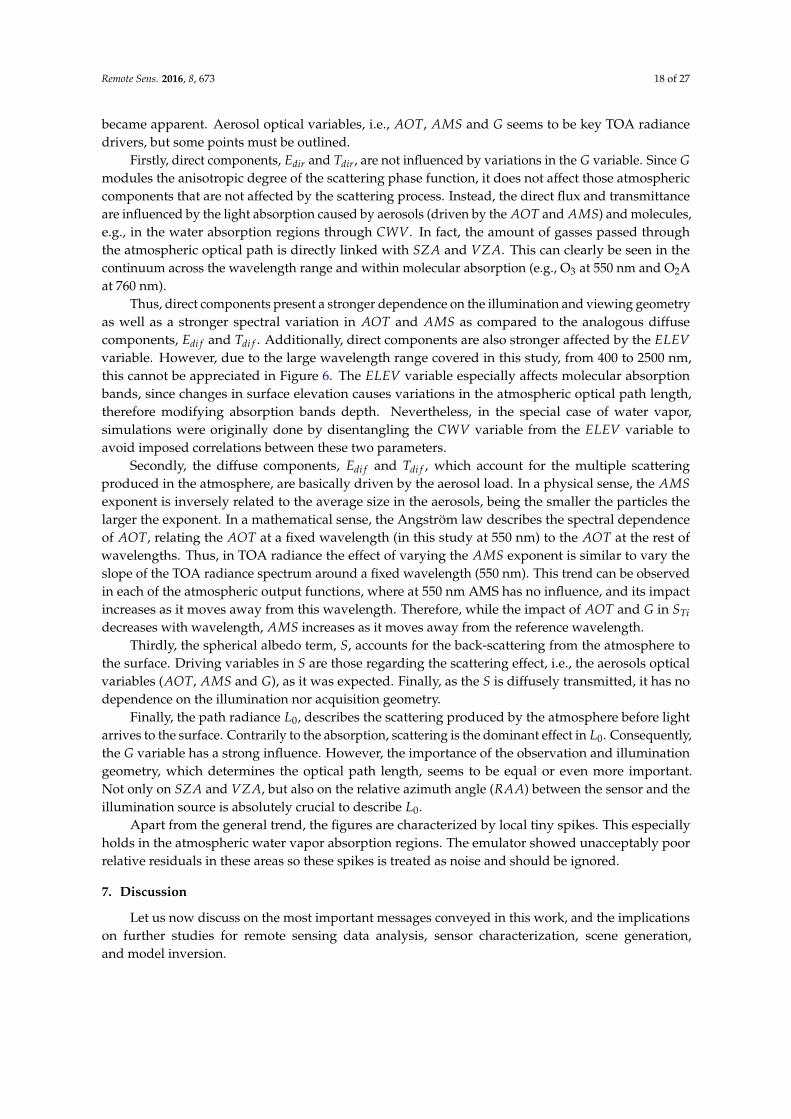
Figure 6. MODTRAN5 GSA STi results according to best performing emulator (see Table 2) for Edi f(GPR: 121 s) (a), Edir (KRR: 101 s) (b), Tdi f (NN: 157 s) (c), Tdir (NN: 151 s) (d), S (NN: 150 s) (e) and L0

(GPR: 166 s) (f) outputs. On top: the used emulator and processing time. s: seconds.

Although a careful interpretation is required in the deep atmospheric water absorption regions,the overall trends of the atmospheric drivers across the 400–2500 nm spectral range emergedcontinuously in general. In all these figures, the relative importance of the atmospheric variables

Remote Sens. 2016, 8, 673 18 of 27

became apparent. Aerosol optical variables, i.e., AOT, AMS and G seems to be key TOA radiancedrivers, but some points must be outlined.

Firstly, direct components, Edir and Tdir, are not influenced by variations in the G variable. Since Gmodules the anisotropic degree of the scattering phase function, it does not affect those atmosphericcomponents that are not affected by the scattering process. Instead, the direct flux and transmittanceare influenced by the light absorption caused by aerosols (driven by the AOT and AMS) and molecules,e.g., in the water absorption regions through CWV. In fact, the amount of gasses passed throughthe atmospheric optical path is directly linked with SZA and VZA. This can clearly be seen in thecontinuum across the wavelength range and within molecular absorption (e.g., O3 at 550 nm and O2Aat 760 nm).

Thus, direct components present a stronger dependence on the illumination and viewing geometryas well as a stronger spectral variation in AOT and AMS as compared to the analogous diffusecomponents, Edi f and Tdi f . Additionally, direct components are also stronger affected by the ELEVvariable. However, due to the large wavelength range covered in this study, from 400 to 2500 nm,this cannot be appreciated in Figure 6. The ELEV variable especially affects molecular absorptionbands, since changes in surface elevation causes variations in the atmospheric optical path length,therefore modifying absorption bands depth. Nevertheless, in the special case of water vapor,simulations were originally done by disentangling the CWV variable from the ELEV variable toavoid imposed correlations between these two parameters.

Secondly, the diffuse components, Edi f and Tdi f , which account for the multiple scatteringproduced in the atmosphere, are basically driven by the aerosol load. In a physical sense, the AMSexponent is inversely related to the average size in the aerosols, being the smaller the particles thelarger the exponent. In a mathematical sense, the Angström law describes the spectral dependenceof AOT, relating the AOT at a fixed wavelength (in this study at 550 nm) to the AOT at the rest ofwavelengths. Thus, in TOA radiance the effect of varying the AMS exponent is similar to vary theslope of the TOA radiance spectrum around a fixed wavelength (550 nm). This trend can be observedin each of the atmospheric output functions, where at 550 nm AMS has no influence, and its impactincreases as it moves away from this wavelength. Therefore, while the impact of AOT and G in STidecreases with wavelength, AMS increases as it moves away from the reference wavelength.

Thirdly, the spherical albedo term, S, accounts for the back-scattering from the atmosphere tothe surface. Driving variables in S are those regarding the scattering effect, i.e., the aerosols opticalvariables (AOT, AMS and G), as it was expected. Finally, as the S is diffusely transmitted, it has nodependence on the illumination nor acquisition geometry.

Finally, the path radiance L0, describes the scattering produced by the atmosphere before lightarrives to the surface. Contrarily to the absorption, scattering is the dominant effect in L0. Consequently,the G variable has a strong influence. However, the importance of the observation and illuminationgeometry, which determines the optical path length, seems to be equal or even more important.Not only on SZA and VZA, but also on the relative azimuth angle (RAA) between the sensor and theillumination source is absolutely crucial to describe L0.

Apart from the general trend, the figures are characterized by local tiny spikes. This especiallyholds in the atmospheric water vapor absorption regions. The emulator showed unacceptably poorrelative residuals in these areas so these spikes is treated as noise and should be ignored.

7. Discussion

Let us now discuss on the most important messages conveyed in this work, and the implicationson further studies for remote sensing data analysis, sensor characterization, scene generation,and model inversion.

Remote Sens. 2016, 8, 673 19 of 27

7.1. Interpreting Emulator Results

Emulation is a technique used to estimate model simulations when the model under investigationis too computationally burdensome to be run many times [34]. Following on initial successfulexperiments that MLRAs can function as emulators to approximate the behavior of physically-basedRTMs [37,38], here the concept of emulating RTMs has been further explored. Specifically, emulatorsapproximating popular RTMs at the leaf, canopy and atmosphere scale were used as input into a GSAscheme. Variance-based GSA methods are excellent tools to identify driving variables in process-basedmodels such as RTMs, but they require many simulations. When models are computationally costly,this method can become cumbersome, and so far only fast RTMs were subject to GSA studies.The excellent emulation-GSA results as compared to the original RTM-GSA results for PROSPECT-4and PROSAIL suggest that emulators can open many practical applications. It demands for a closerinspection of their properties.

When it comes to emulating RTM spectral ouptuts, an important aspect involves dealing witha large amount of multi-outputs, e.g., up to 2101 wavebands to construct the 400–2500 nm profilesat 1 nm. It made that existing emulation packages (e.g., BACCO (Bayesian Analysis of ComputerCode Outputs) or GEM-SA (Gaussian Emulation Machine for Sensitivity Analysis) [34,72,73]), as theyprocess only one output, are impractical for RTM sensitivity analysis. To cope with such a highdegree of multiple-output, we had implemented a PCA dimensionality reduction procedure intoARTMO’s Emulator toolbox and linked it with the GSA toolbox. The Emulator toolbox is essentiallynothing more than a collection of multivariate regression algorithms that builds a relationship betweenRTM input variables and spectral output. Any multivariate regression algorithm can potentiallyfunction as emulator. However, the regression methods should be able to implement nonlinear andsmooth (regularized) functions, in order to deal with complex, possibly ill-posed input-output relations.Earlier experiments on emulation revealed that nonparametric regression methods limited to lineartransformations, such as partial least square regression (PLSR), are unable to reconstruct spectralsignals with sufficient accuracy [37], while nonlinear regression methods in the families of NNs andkernel-based MLRAs have proven to be powerful adaptive estimators (e.g., [5,37,46]).

In this study three potentially powerful MLRAs (KRR, NN and GPR) were evaluated to actas emulators on their accuracy accuracy, computational burden and correlation of the residuals.Goodness-of-fit validation results indicated that relative errors (i.e., NRMSE) were below 0.5%.Nevertheless, although trained extremely fast (about 2 s), KRR performed mostly worse, partly due tothe low number of hyperparemeters used in defining the kernel function. NN performed generallysuperior but this method requires a considerably longer training phase, here up to 14 min, which maybe unacceptably long when dealing with computationally cheap RTMs. Consequently, for applicationsbased on PROSPECT and SAIL, most likely it does not pay off to emulate them with NN, e.g., here theoriginal PROSPECT and PROSAIL GSA procedures were completed faster than the NN training plusNN-GSA running. In turn, a training phase in the order of minutes may not be trivial when it comes tocostly RTMs. For instance, one single MODTRAN5 simulation at finest spectral resolution of 0.1 cm−1

may take over 10 min on a contemporary computer. GPR may function as an sensible compromise;it is relatively fast in training (here less than 2 min), fast in testing, and with accuracies generally closeto those of NN.

Moreover, GPR possesses additional properties which were not explored in this paper andthat explain its first choice for emulation (e.g., [34,74]). GPR can give some information about therelative relevance of the inputs, it can provide associated uncertainty intervals (referred to as codeuncertainty of the emulator) for the predictions, and the Jacobian and Hessians of the predictionfunction can be explicitly derived [50,75]. The uncertainty estimations can be of interest as theyprovide a reliable indication of the trustworthiness of the generated outputs. For instance, in regionswhere the RTM is not evaluated, we are uncertain about what the true simulator would introduce,and thus uncertainties are larger than within the training variable space. Accordingly, code uncertaintycan be reduced by increasing our knowledge of the RTM, i.e., by increasing the training sample size [76].

Remote Sens. 2016, 8, 673 20 of 27

In fact, the uncertainty intervals can function as a quality check, e.g., accepting only emulations withina confidence threshold. Nevertheless, it should be noted that preparatory experiments with PROSPECTand SAIL revealed that these uncertainties are generally so small that they were hardly apparent (resultsnot shown), as has also been recently observed by [38].

However, this does not mean that emulators are free from limitations. Emulators are meta-models,i.e., model of a model, implying that they only approximate the functioning of the simulator, i.e.,the RTM. It bears the following consequences: (1) the emulator can only be as good as the simulator, i.e.,imperfections in the simulator are mirrored to the emulator; (2) the accuracy of the emulator depend onthe type of machine learning regression and the number and representativity of the training samples;and (3) emulators uncertainty increases when moving beyond the boundaries of the training datasetso accurate extrapolation is compromised. All in all, a careful training and validation of emulatorsis strictly necessary, and associated uncertainty intervals may help deducing whether the generatedoutput is within reasonable and physically meaningful levels.

7.2. Interpreting Sensitivity Analysis Results

Machine learning emulators provided accurate estimations and reproduced the underlyingmechanistic principles encoded in the RTMs, and allowed for intensive simulations and remotesensing applications. By applying Saltelli’s GSA scheme, we studied the total sensitivity providedby the emulators compared against RTM reference results for PROSPECT-4 and PROSAIL. Resultsdemonstrated that the emulator-GSA setup delivers identical sensitivity patterns as the original RTMGSA scheme. Nevertheless, given that these two RTMs are computationally cheap, the gain in speedto deliver the sensitivity results is not very large. If computationally cheap, obviously, applying GSAto the original RTMs is always preferred. Conversely, the use of emulators can become a powerful toolto bypass the computational burden of expensive RTMs. For instance, the emulator-GSA setup allowsfor the first time decomposing MODTRAN5 outputs into its driving input variables across the spectralrange. Here, for multiple MODTRAN5 atmospheric transfer functions (i.e., MODTRAN5 outputs) theemulator-GSA setup quantified the key variables within reasonable time, i.e., on the order of minutes.To put in perspective, conducting the same analysis with original MODTRAN5 simulations wouldhave taken about 47 days on the same computer.

The MODTRAN5 emulation-GSA STi results showed that the relative importance of each inputvariable in the atmospheric transfer functions were physically meaningful: e.g., effect of water vapor inthese absorption bands, effect of scattering variables in diffuse irradiance and transmittance. However,unlike leaf and canopy surface reflectance, the spectrum of the atmospheric transfer functions is affectedby many narrow atmospheric and solar absorption bands on top of a smooth curve. The analysis ofthe residuals indicates that the emulators performed well in the smoother regions of the spectrum,while they showed large relative errors within the narrow atmospheric absorption regions withvalues close to zero. Most noticeable are the dominant water vapor absorption regions around1400 and 1900 nm, which are typically discarded in further processing. In fact, we had repeated theemulation-GSA analysis but then without those absorption regions (results not shown). It led to thesame sensitivity patterns but then with gaps where the data was removed. However, the relevantinformation that these regions are largely driven by CWV (especially for Edir and Tdir) would then beomitted. Despite high uncertainties, we therefore preferred to include the whole spectrum for sakeof completeness. To analyze atmospheric drivers further, we consider as further work to dedicatedifferent emulators (with dedicated principal components) for distinctive absorption regions to bettercapture high frequency spectral details. Another future sensitivity analysis would include moreMODTRAN input variables. While here only the most relevant atmospheric variables are studied,it is of interest to disentangle the role of other variables such as single scattering albedo or even thevariables that allow modelling the aerosol vertical distribution as a bi-modal, log-normal or gammafunction [77].

Remote Sens. 2016, 8, 673 21 of 27

For practical remote sensing applications, the PROSAIL and MODTRAN STi results suggest thatnot all input variables are equally important in shaping spectral output. A few variables possesshardly any sensitivity, which implies they can be safely kept to default values e.g., skyl and RAAfor PROSAIL. In the particular case of MODTRAN5, the driving input variables must be separatelystudied for each atmospheric function. On the whole, ELEV and also RAA (apart from L0) have hardlyimpact. However, more importantly, some variables play only a role in specific absorption regions,such as CWV. This suggests that CWV can be kept as constant e.g., when interested in analyzingscattering effects in the blue region. In fact, ELEV and sun-target-sensor geometry (VZA, SZA andRAA) are typically known and thus kept fixed in applications. Similarly, by discarding insensitivevariables from the sampling scheme it is possible to simplify the computational load and inversionproblem for mapping applications (e.g., as in [26,78]).

Finally, it must be noted that the RTM input variables are independent, i.e., no physical linksbetween them have been introduced, although in reality they can be correlated. For instance, in caseof MODTRAN5 the impact of the ELEV variable appears negligible for all atmospheric functions.However, in reality surface elevation drives the atmospheric optical path, and ELEV is therefore tosome extent correlated with the amount of the atmospheric absorbers (gaseous components) such aswater vapor. Similarly, in reality leaf and canopy variables are to some extent correlated, e.g., Cab occurswith Cw, and the existence leaf optical properties automatically imply the existence of leaves thusLAI (e.g., [79]). Accordingly, when aiming for practical applications from sensitivity studies it isrecommendable to filter out input combinations that are unlikely to occur in reality.

7.3. New Processing Opportunities with Emulators

Probably the most significant advantage of emulators is the tremendous gain in processingspeed. Each of the tested emulators delivers outputs quasi-instantly, which implies boosting inprocessing speed in the orders of tens to ten thousands depending on the speed of the originalRTM. For instance, for the computationally intensive atmospheric RTM MODTRAN, the gain isabout 130,000. At the same time, they hardly take memory space, only a few model coefficients arestored for prediction. Consequently, emulators can become an attractive technique for a diversity ofremote sensing applications beyond GSA studies, which are briefly outlined in what follows.

Numerical inversion. Iterative optimization is a classical technique to invert RTMs in RS [80,81]. Theoptimization consists in minimizing a cost function, which estimates the difference between measuredand estimated variables by successive input variable iteration. The iterative optimization algorithmsare computationally demanding and hence time-consuming when large remotely-sensed datasets areinverted. This method has never been a viable option for computationally intensive RTMs, and evenfor computationally cheap RTMs the method is slow and not appealing. Making use of pre-generatedLUTs is preferred in inversion schemes (see [5] for a review). For instance, canopy RTM LUTs are usedin the MODIS LAI retrieval products [82] and also atmospheric correction algorithms make use ofLUT-based inversion methods (e.g., [83–87]). Accordingly, when replacing the original RTMs by theiremulated counterparts then numerical inversion can again become an attractive alternative; numericalinversion using a RTM-like emulator can go very fast. It would bypass the need to invest in large andheavy LUTs. To explore this research line further, a so-called Numerical Inversion Toolbox is currentlyunder construction that will make use of emulators.

Scene generation. Forthcoming optical satellite missions increasingly make use of end-to-endmission performance simulators (E2ES) to generate simulated scenes as would be detected by theoptical sensor (e.g., [9,88]). A drawback is that scene rendering can take a long processing time,especially when based on computationally expensive models such as SCOPE or MODTRAN [89].Accordingly, when replacing the original RTMs by their emulated counterparts then scenes can begenerated rapidly. Within the framework of ESA’s forthcoming 8th Earth Explorer FLEX, currently it isbeing investigated whether some tedious parts of the FLEX-E2ES scene generation can be replacedby emulators.

Remote Sens. 2016, 8, 673 22 of 27

Data assimilation schemes. Data assimilation schemes where multiple data sources and models arecoupled are more commonly applied in climate and Earth system studies. Often they use advanceddata fusion and processing techniques, e.g., Ensemble Kalman Filter and Markov Chain Monte Carlomethods (e.g., [90–92]) that can take considerable computational time and so the limiting factor inthe processing chain. To mitigate the processing bottlenecks in assimilation schemes, it has beenproposed to replace parts of deterministic input-output processing chain by emulators. Typicallythe most computationally burdensome parts, although in does not have be one emulator attemptingto emulate the complete system, but rather replacing tedious parts by multiple smaller but highlyaccurate emulators. Efforts in this direction are undertaken by [38,93].

Improved emulators. From a pure machine learning point of view, emulators boil down todeveloping regression algorithms that should be accurate enough when training with relativelyfew-to-moderate available observations. The scenario calls for the concept of regularization,which is tightly related to invariance encoding and incorporation of prior knowledge and thedefinition of sensible cost functions. Many opportunities appear here to improve the performance ofemulators: one could think of including multiple pieces of information in the regression algorithmwith multimodal/multiresolution regression, e.g., by combining RTMs for the same problem,to accommodate spatial or temporal relations in the emulation [44,94], and to implement betterdimensionality reduction techniques beyond linear PCA to deal with the multi-output problem [95].Apart from these improvements in the regression algorithm, we raise here the important issueof assessment of the emulator function, e.g., by looking at the Jacobian and Hessian of thetransformation [38,96], Bayesian sensitivity analysis [34,97], as well as developing emulators thatmay deal with coupled RTMs and transformations of coefficients [50].

8. Conclusions

Emulators are statistical constructs that approximate the functioning of process-based modelssuch as RTMs. They provide great savings in memory and tremendous gains in processing speed,while yielding competitive accuracies in reconstructing RTM outputs. This emulation technique opensmany new research and practical opportunities, not in the least enabling to convert computationallyexpensive RTMs into computationally fast surrogate models.

As a proof-of-concept, we demonstrated the use of emulated RTMs into a global sensitivityanalysis (GSA) study. We analyzed three MLRAs (NN, KRR and GPR) on their ability to function asan emulator to approximate spectral outputs of the leaf optical RTM PROSPECT-4, the canopy RTMPROSAIL and the computational expense atmospheric RTM MODTRAN5. A PCA preprocessing stepwas introduced to speed up processing and enable deconstructing the full spectral profile. ParticularlyNN and GPR proved to act as accurate emulators, with normalized root-mean-squared errors below0.2% for the majority of RTM validation datasets. The PROSPECT-4 and PROSAIL-like emulators weresubsequently implemented into a GSA scheme. Because of delivering accurate RTM reflectance outputs,NN and GPR emulators delivered GSA total order sensitivity (STi) results (including interactions)identical as the reference STi results coming from original PROSPECT-4 and PROSAIL simulations.

These two studies successfully demonstrated the benefit and reliability of using emulators intoGSA studies. As a next step, the most accurate MODTRAN5-like emulators for six MODTRAN5atmospheric transfer outputs (Edi f , Edir, Tdi f , Tdir, S and L0) were implemented into the GSA scheme.The analysis along the 400–2500 nm spectral range did not take more than a few minutes. Key drivingatmospheric variables were identified. Particularly the aerosol optical variables are mostly drivingthe entire spectral range. While AOT and AMS govern all atmospheric outputs, the asymmetrycoefficient of scattering G, only impacts those outputs diffusely transmitted. On the contrary, molecularcompounds such as CWV, which only affects specific absorption regions, present a stronger effect onthose outputs that are directly transmitted.

Remote Sens. 2016, 8, 673 23 of 27

Altogether, these GSA studies at the leaf, canopy and atmosphere scale demonstrated that theemulator technique, in which both consistent physical assumptions and statistical learning live together,can open many new opportunities in the use of advanced RTMs for practical applications.

Acknowledgments: This work was partially supported by the European Space Agency under project ’FLEX-BridgeStudy’ (ESA contract RFP IPL-PEO/FF/lf/14.687), the ERDF and the Spanish Ministry of Economyand Competitiveness under project TIN2015-64210-R. Gustau Camps-Valls wants to thank the EuropeanResearch Council (ERC) funding under the ERC-CoG-2014 SEDAL under grant agreement 647423. We alsothank José Gómez-Dans for valuable discussions on emulation. We thank the four reviewers for theirvaluable suggestions.

Author Contributions: J.V., N.S. and J.V. designed and carried out the experiments, and wrote the manuscript.J.P.R. developed the Emulator toolbox. J.M.-M., G.C.-V. and J.M. contributed to the drafting of the manuscript.

Conflicts of Interest: The authors declare no conflict of interest.

References

1. Zhang, Y.; Rossow, W.; Lacis, A.; Oinas, V.; Mishchenko, M. Calculation of radiative fluxes from the surfaceto top of atmosphere based on ISCCP and other global data sets: Refinements of the radiative transfer modeland the input data. J. Geophys. Res. D Atmos. 2004, 109, doi:10.1029/2003JD004457.

2. Jacquemoud, S.; Verhoef, W.; Baret, F.; Bacour, C.; Zarco-Tejada, P.; Asner, G.; François, C.; Ustin, S.PROSPECT + SAIL models: A review of use for vegetation characterization. Remote Sens. Environ. 2009,113, S56–S66.

3. Deiveegan, M.; Balaji, C.; Venkateshan, S. A polarized microwave radiative transfer model for passiveremote sensing. Atmos. Res. 2008, 88, 277–293.

4. Van der Tol, C.; Berry, J.A.; Campbell, P.K.E.; Rascher, U. Models of fluorescence and photosynthesis forinterpreting measurements of solar-induced chlorophyll fluorescence. J. Geophys. Res. Biogeosci. 2014, 119,2312–2327.

5. Verrelst, J.; Camps-Valls, G.; Muñoz-Marí, J.; Rivera, J.; Veroustraete, F.; Clevers, J.; Moreno, J. Optical remotesensing and the retrieval of terrestrial vegetation bio-geophysical properties—A review. ISPRS J. Photogramm.Remote Sens. 2015, 108, 273–290.

6. Verhoef, W.; Bach, H. Simulation of Sentinel-3 images by four-stream surface-atmosphere radiative transfermodeling in the optical and thermal domains. Remote Sens. Environ. 2012, 120, 197–207.

7. Meharrar, K.; Bachari, N. Modelling of radiative transfer of natural surfaces in the solar radiation spectrum:Development of a satellite data simulator (SDDS). Int. J. Remote Sens. 2014, 35, 1199–1216.

8. Segl, K.; Guanter, L.; Rogass, C.; Kuester, T.; Roessner, S.; Kaufmann, H.; Sang, B.; Mogulsky, V.; Hofer, S.EeteSThe EnMAP end–to–end simulation tool. IEEE J. Sel. Top. Appl. Earth Obs. Remote Sens. 2012, 5,522–530.

9. Vicent, J.; Sabater, N.; Tenjo, C.; Acarreta, J.; Manzano, M.; Rivera, J.; Jurado, P.; Franco, R.; Alonso, L.;Verrelst, J.; et al. FLEX End-to-End Mission Performance Simulator. IEEE Trans. Geosci. Remote Sens. 2016,54, 4215–4223.

10. Widlowski, J.L.; Taberner, M.; Pinty, B.; Bruniquel-Pinel, V.; Disney, M.; Fernandes, R.; Gastellu-Etchegorry, J.P.;Gobron, N.; Kuusk, A.; Lavergne, T.; et al. Third Radiation Transfer Model Intercomparison (RAMI) exercise:Documenting progress in canopy reflectance models. J. Geophys. Res. Atmos. 2007, 112, doi:10.1029/2006JD007821.

11. Baret, F.; Buis, S. Estimating canopy characteristics from remote sensing observations. Review of methodsand associated problems. In Advances in Land Remote Sensing: System, Modeling, Inversion and Application;Liang, S., Ed.; Springer: Berlin/Heidelberg, Germany, 2008; pp. 171–200.

12. Widlowski, J.L.; Pinty, B.; Lopatka, M.; Atzberger, C.; Buzica, D.; Chelle, M.; Disney, M.; Gastellu-Etchegorry, J.P.;Gerboles, M.; Gobron, N.; et al. The fourth radiation transfer model intercomparison (RAMI-IV): Proficiencytesting of canopy reflectance models with ISO-13528. J. Geophys. Res. Atmos. 2013, 118, 6869–6890.

13. Widlowski, J.L.; Mio, C.; Disney, M.; Adams, J.; Andredakis, I.; Atzberger, C.; Brennan, J.; Busetto, L.; Chelle, M.;Ceccherini, G.; et al. The fourth phase of the radiative transfer model intercomparison (RAMI) exercise:Actual canopy scenarios and conformity testing. Remote Sens. Environ. 2015, 169, 418–437.

Remote Sens. 2016, 8, 673 24 of 27

14. Feret, J.B.; François, C.; Asner, G.P.; Gitelson, A.A.; Martin, R.E.; Bidel, L.P.R.; Ustin, S.L.; le Maire, G.;Jacquemoud, S. PROSPECT-4 and 5: Advances in the leaf optical properties model separating photosyntheticpigments. Remote Sens. Environ. 2008, 112, 3030–3043.

15. Verhoef, W. Light scattering by leaf layers with application to canopy reflectance modeling: The SAIL model.Remote Sens. Environ. 1984, 16, 125–141.

16. Vermote, E.; Tanré, D.; Deuzé, J.; Herman, M.; Morcrette, J.J. Second simulation of the satellite signal in thesolar spectrum, 6S: An overview. IEEE Trans. Geosci. Remote Sens. 1997, 35, 675–686.

17. Lipton, A.; Moncet, J.L.; Boukabara, S.A.; Uymin, G.; Quinn, K. Fast and accurate radiative transfer in themicrowave with optimum spectral sampling. IEEE Trans. Geosci. Remote Sens. 2009, 47, 1909–1917.

18. Govaerts, Y.M.; Verstraete, M.M. Raytran: A Monte Carlo ray-tracing model to compute light scattering inthree-dimensional heterogeneous media. IEEE Trans. Geosci. Remote Sens. 1998, 36, 493–505.

19. North, P. Three-dimensional forest light interaction model using a Monte Carlo method. IEEE Trans. Geosci.Remote Sens. 1996, 34, 946–956.

20. Lewis, P. Three-dimensional plant modelling for remote sensing simulation studies using the Botanical PlantModelling System. Agronomie 1999, 19, 185–210.

21. Gastellu-Etchegorry, J.; Demarez, V.; Pinel, V.; Zagolski, F. Modeling radiative transfer in heterogeneous 3-Dvegetation canopies. Remote Sens. Environ. 1996, 58, 131–156.

22. Petropoulos, G.; Wooster, M.; Carlson, T.; Kennedy, M.; Scholze, M. A global Bayesian sensitivity analysisof the 1D SimSphere soil vegetation atmospheric transfer (SVAT) model using Gaussian model emulation.Ecol. Model. 2009, 220, 2427–2440.

23. Van Der Tol, C.; Verhoef, W.; Timmermans, J.; Verhoef, A.; Su, Z. An integrated model of soil-canopy spectralradiances, photosynthesis, fluorescence, temperature and energy balance. Biogeosciences 2009, 6, 3109–3129.

24. Berk, A.; Anderson, G.; Acharya, P.; Bernstein, L.; Muratov, L.; Lee, J.; Fox, M.; Adler-Golden, S.; Chetwynd, J.;Hoke, M.; et al. MODTRANTM5: 2006 update. In Proceedings of the Algorithms and Technologies forMultispectral, Hyperspectral, and Ultraspectral Imagery XII, Orlando, FL, USA, 17 April 2006; Volume 6233.

25. España, M.; Baret, F.; Aries, F.; Chelle, M.; Andrieu, B.; Prévot, L. Modeling maize canopy 3D architecture:Application to reflectance simulation. Ecol. Model. 1999, 122, 25–43.

26. Mousivand, A.; Menenti, M.; Gorte, B.; Verhoef, W. Multi-temporal, multi-sensor retrieval of terrestrialvegetation properties from spectral-directional radiometric data. Remote Sens. Environ. 2015, 158, 311–330.

27. Saltelli, A.; Ratto, M.; Andres, T.; Campolongo, F.; Cariboni, J.; Gatelli, D.; Saisana, M.; Tarantola, S.Global Sensitivity Analysis: The Primer; John Wiley & Sons: Hoboken, NJ, USA, 2008.

28. Yang, J. Convergence and uncertainty analyses in Monte-Carlo based sensitivity analysis. Environ. Model. Softw.2011, 26, 444–457.

29. Nossent, J.; Elsen, P.; Bauwens, W. Sobol’sensitivity analysis of a complex environmental model.Environ. Model. Softw. 2011, 26, 1515–1525.

30. Bowyer, P.; Danson, F. Sensitivity of spectral reflectance to variation in live fuel moisture content at leaf andcanopy level. Remote Sens. Environ. 2004, 92, 297–308.

31. Stuckens, J.; Verstraeten, W.W.; Delalieux, S.; Swennen, R.; Coppin, P. A dorsiventral leaf radiative transfermodel: Development, validation and improved model inversion techniques. Remote Sens. Environ. 2009,113, 2560–2573.

32. Mousivand, A.; Menenti, M.; Gorte, B.; Verhoef, W. Global sensitivity analysis of the spectral radiance ofa soil–vegetation system. Remote Sens. Environ. 2014, 145, 131–144.

33. Verrelst, J.; Rivera, J.; Van Der Tol, C.; Magnani, F.; Mohammed, G.; Moreno, J. Global sensitivity analysis ofthe SCOPE model: What drives simulated canopy-leaving sun-induced fluorescence? Remote Sens. Environ.2015, 166, 8–21.

34. O’Hagan, A. Bayesian analysis of computer code outputs: A tutorial. Reliab. Eng. Syst. Saf. 2006, 91,1290–1300.

35. Rohmer, J.; Foerster, E. Global sensitivity analysis of large-scale numerical landslide models based onGaussian-Process meta-modeling. Comput. Geosci. 2011, 37, 917–927.

36. Bounceur, N.; Crucifix, M.; Wilkinson, R. Global sensitivity analysis of the climate–vegetation system toastronomical forcing: An emulator-based approach. Earth Syst. Dyn. Discuss. 2014, 5, 901–943.

37. Rivera, J.P.; Verrelst, J.; Gómez-Dans, J.; Muñoz Marí, J.; Moreno, J.; Camps-Valls, G. An Emulator Toolbox toApproximate Radiative Transfer Models with Statistical Learning. Remote Sens. 2015, 7, 9347.

Remote Sens. 2016, 8, 673 25 of 27

38. Gómez-Dans, J.L.; Lewis, P.E.; Disney, M. Efficient Emulation of Radiative Transfer Codes Using GaussianProcesses and Application to Land Surface Parameter Inferences. Remote Sens. 2016, 8, 119.

39. Carnevale, C.; Finzi, G.; Guariso, G.; Pisoni, E.; Volta, M. Surrogate models to compute optimal air qualityplanning policies at a regional scale. Environ. Model. Softw. 2012, 34, 44–50.

40. Villa-Vialaneix, N.; Follador, M.; Ratto, M.; Leip, A. A comparison of eight metamodeling techniques for thesimulation of N2O fluxes and N leaching from corn crops. Environ. Model. Softw. 2012, 34, 51–66.

41. Castelletti, A.; Galelli, S.; Ratto, M.; Soncini-Sessa, R.; Young, P. A general framework for dynamic emulationmodelling in environmental problems. Environ. Model. Softw. 2012, 34, 5–18.

42. Lee, L.; Pringle, K.; Reddington, C.; Mann, G.; Stier, P.; Spracklen, D.; Pierce, J.; Carslaw, K. The magnitudeand causes of uncertainty in global model simulations of cloud condensation nuclei. Atmos. Chem. Phys.2013, 13, 8879–8914.

43. Ireland, G.; Petropoulos, G.; Carlson, T.; Purdy, S. Addressing the ability of a land biosphere model to predictkey biophysical vegetation characterisation parameters with Global Sensitivity Analysis. Environ. Model. Softw.2015, 65, 94–107.

44. Camps-Valls, G.; Bruzzone, L. (Eds.) Kernel Methods for Remote Sensing Data Analysis; Wiley & SonsLtd.: Chichester, UK, 2009.

45. Razavi, S.; Tolson, B.A.; Burn, D.H. Numerical assessment of metamodelling strategies in computationallyintensive optimization. Environ. Model. Softw. 2012, 34, 67–86.

46. Verrelst, J.; Muñoz, J.; Alonso, L.; Delegido, J.; Rivera, J.; Camps-Valls, G.; Moreno, J. Machine learningregression algorithms for biophysical parameter retrieval: Opportunities for Sentinel-2 and -3. Remote Sens.Environ. 2012, 118, 127–139.

47. Rivera, J.; Verrelst, J.; Delegido, J.; Veroustraete, F.; Moreno, J. On the semi-automatic retrieval of biophysicalparameters based on spectral index optimization. Remote Sens. 2014, 6, 4924–4951.

48. Wold, S.; Esbensen, K.; Geladi, P. Principal component analysis. Chemom. Intell. Lab. Syst. 1987, 2, 37–52.49. Camps-Valls, G.; Muñoz-Marí, J.; Gómez-Chova, L.; Guanter, L.; Calbet, X. Nonlinear statistical retrieval of

atmospheric profiles from MetOp-IASI and MTG-IRS infrared sounding data. IEEE Trans. Geosci. Remote Sens.2012, 50, 1759–1769.

50. Camps-Valls, G.; Verrelst, J.; Muñoz-Marí, J.; Laparra, V.; Mateo-Jiménez, F.; Gómez-Dans, J. A Survey onGaussian Processes for Earth Observation Data Analysis. IEEE Geosci. Remote Sens. Mag. 2016, 4, 58–78.

51. Camps-Valls, G.; Gómez-Chova, L.; Muñoz-Marí, J.; Lázaro-Gredilla, M.; Verrelst, J. SimpleR: A SimpleEducational Matlab Toolbox for Statistical Regression, 2013. Available online: http://isp.uv.es/soft_regression.html (accessed on 18 August 2016).

52. Sobol’, I.M. On sensitivity estimation for nonlinear mathematical models. Mat. Model. 1990, 2, 112–118.53. McRae, G.J.; Tilden, J.W.; Seinfeld, J.H. Global sensitivity analysis—A computational implementation of the

Fourier amplitude sensitivity test (FAST). Comput. Chem. Eng. 1982, 6, 15–25.54. Saltelli, A.; Annoni, P.; Azzini, I.; Campolongo, F.; Ratto, M.; Tarantola, S. Variance based sensitivity analysis

of model output. Design and estimator for the total sensitivity index. Comput. Phys. Commun. 2010, 181,259–270.

55. Song, X.; Bryan, B.A.; Paul, K.I.; Zhao, G. Variance-based sensitivity analysis of a forest growth model.Ecol. Model. 2012, 247, 135–143.

56. Saltelli, A.; Annoni, P. How to avoid a perfunctory sensitivity analysis. Environ. Model. Softw. 2010, 25,1508–1517.

57. Saltelli, A. Making best use of model evaluations to compute sensitivity indices. Comput. Phys. Commun.2002, 145, 280–297.

58. Verhoef, W.; Jia, L.; Xiao, Q.; Su, Z. Unified optical-thermal four-stream radiative transfer theory forhomogeneous vegetation canopies. IEEE Trans. Geosci. Remote Sens. 2007, 45, 1808–1822.

59. Wang, P.; Liu, K.Y.; Cwik, T.; Green, R. MODTRAN on supercomputers and parallel computers.Parallel Comput. 2002, 28, 53–64.

60. Stamnes, K.; Tsay, S.C.; Wiscombe, W.; Jayaweera, K. Numerically stable algorithm for discrete-ordinate-methodradiative transfer in multiple scattering and emitting layered media. Appl. Opt. 1988, 27, 2502–2509.

61. Goody, R.; West, R.; Chen, L.; Crisp, D. The correlated-k method for radiation calculations in nonhomogeneousatmospheres. J. Quant. Spectrosc. Radiat. Transf. 1989, 42, 539–550.

Remote Sens. 2016, 8, 673 26 of 27

62. Berk, A.; Anderson, G.; Acharya, P.; Shettle, E. MODTRAN 5.2.1 User’s Manual; Spectral Science Inc.:Burlingtonm, MA, USA, 2011.

63. Guanter, L.; Richter, R.; Kaufmann, H. On the application of the MODTRAN4 atmospheric radiative transfercode to optical Remote Sensing. Int. J. Remote Sens. 2009, 30, 1407–1424.

64. Richter, R.; Schläpfer, D. Geo-atmospheric processing of airborne imaging spectrometry data. Part 2:Atmospheric/topographic correction. Int. J. Remote Sens. 2002, 23, 2631–2649.

65. Cooley, T.; Anderson, G.; Felde, G.; Hoke, M.; Ratkowski, A.; Chetwynd, J.; Gardner, J.; Adler-Golden, S.;Matthew, M.; Berk, A.; et al. FLAASH, a MODTRAN4-based atmospheric correction algorithm,its applications and validation. In IEEE International Geoscience and Remote Sensing Symposium; IEEE:Piscataway, NJ, USA, 2002; Volume 3, pp. 1414–1418.

66. Guanter, L. New Algorithms for Atmospheric Correction and Retrieval of Biophysical Parameters in EarthObservation: Application to ENVISAT/MERIS Data, 2006. Available online: http://hdl.handle.net/10803/9877 (accessed on 18 August 2016).

67. Berk, A.; Acharya, P.; Anderson, G.; Gossage, B. Recent developments in the MODTRAN atmospheric modeland implications for hyperspectral compensation. In 2009 IEEE International Geoscience and Remote SensingSymposium; IEEE: Piscataway, NJ, USA, 2009; Volume 2, pp. II262–II265.

68. Verrelst, J.; Romijn, E.; Kooistra, L. Mapping vegetation density in a heterogeneous river floodplainecosystem using pointable CHRIS/PROBA data. Remote Sens. 2012, 4, 2866–2889.

69. Verrelst, J.; Rivera, J.; Moreno, J. ARTMO’s Global Sensitivity Analysis (GSA) toolbox to quantify drivingvariables of leaf and canopy radiative transfer models. EARSeL eProc. 2015, 14, 1–11.

70. McKay, M.; Beckman, R.; Conover, W. Comparison of three methods for selecting values of input variablesin the analysis of output from a computer code. Technometrics 1979, 21, 239–245.

71. Conti, S.; O’Hagan, A. Bayesian emulation of complex multi-output and dynamic computer models. J. Stat.Plan. Inference 2010, 140, 640–651.

72. Kennedy, M.; O’Hagan, A. Bayesian calibration of computer models. J. R. Stat. Soc. Ser. B Stat. Methodol.2001, 63, 425–450.

73. Hankin, R.K. Introducing BACCO, an R package for Bayesian analysis of computer code output. J. Stat. Softw.2005, 14, 1–21.

74. Conti, S.; Gosling, J.; Oakley, J.; O’Hagan, A. Gaussian process emulation of dynamic computer codes.Biometrika 2009, 96, 663–676.

75. Verrelst, J.; Alonso, L.; Camps-Valls, G.; Delegido, J.; Moreno, J. Retrieval of vegetation biophysicalparameters using Gaussian process techniques. IEEE Trans. Geosci. Remote Sens. 2012, 50, 1832–1843.

76. Verrelst, J.; Rivera, J.; Moreno, J.; Camps-Valls, G. Gaussian processes uncertainty estimates in experimentalSentinel-2 LAI and leaf chlorophyll content retrieval. ISPRS J. Photogramm. Remote Sens. 2013, 86, 157–167.

77. Hansen, J.E.; Travis, L.D. Light scattering in planetary atmospheres. Space Sci. Rev. 1974, 16, 527–610.78. Verrelst, J.; van der Tol, C.; Magnani, F.; Sabater, N.; Rivera, J.; Mohammed, G.; Moreno, J. Evaluating the

predictive power of sun-induced chlorophyll fluorescence to estimate net photosynthesis of vegetationcanopies: A SCOPE modeling study. Remote Sens. Environ. 2016, 176, 139–151.

79. Ollinger, S. Sources of variability in canopy reflectance and the convergent properties of plants. New Phytol.2011, 189, 375–394.

80. Jacquemoud, S.; Baret, F.; Andrieu, B.; Danson, F.; Jaggard, K. Extraction of vegetation biophysical parametersby inversion of the PROSPECT + SAIL models on sugar beet canopy reflectance data. Application to TMand AVIRIS sensors. Remote Sens. Environ. 1995, 52, 163–172.

81. Kuusk, A. Monitoring of vegetation parameters on large areas by the inversion of a canopy reflectancemodel. Int. J. Remote Sens. 1998, 19, 2893–2905.

82. Myneni, R.; Hoffman, S.; Knyazikhin, Y.; Privette, J.; Glassy, J.; Tian, Y.; Wang, Y.; Song, X.; Zhang, Y.;Smith, G.; et al. Global products of vegetation leaf area and fraction absorbed PAR from year one ofMODIS data. Remote Sens. Environ. 2002, 83, 214–231.

83. Richter, R. A spatially adaptive fast atmospheric correction algorithm. Int. J. Remote Sens. 1996, 17, 1201–1214.84. Thome, K.; Palluconi, F.; Takashima, T.; Masuda, K. Atmospheric correction of ASTER. IEEE Trans. Geosci.

Remote Sens. 1998, 36, 1199–1211.85. Kotchenova, S.; Vermote, E.; Matarrese, R.; Klemm, F., Jr. Validation of a vector version of the 6S radiative

transfer code for atmospheric correction of satellite data. Part I: Path radiance. Appl. Opt. 2006, 45, 6762–6774.

Remote Sens. 2016, 8, 673 27 of 27

86. Guanter, L.; Alonso, L.; Moreno, J. CHRIS Proba Atmospheric Correction Module. Availableonline: http://www.brockmann-consult.de/beam-wiki/download/attachments/32964611/chrisbox-atmospheric_correction_atbd-2.0.pdf (accessed on 2 June 2012).

87. Hagolle, O.; Huc, M.; Pascual, D.; Dedieu, G. A multi-temporal and multi-spectral method to estimateaerosol optical thickness over land, for the atmospheric correction of FormoSat-2, LandSat, VENµS andSentinel-2 images. Remote Sens. 2015, 7, 2668–2691.

88. Segl, K.; Guanter, L.; Gascon, F.; Kuester, T.; Rogass, C.; Mielke, C. S2eteS: An End-to-End Modeling Tool forthe Simulation of Sentinel-2 Image Products. IEEE Trans. Geosci. Remote. Sens. 2015, 53, 5560–5571.

89. Rivera, J.; Sabater, N.; Tenjo, C.; Vicent, J.; Moreno, J. Synthetic scene simulator for hyperspectral spacebornepassive optical sensors. Application to ESA’s FLEX/Sentinel-3 tandem mission. In Proceedings of theWHISPERS—6th Workshop on Hyperspectral Image and Signal: Evolution in Remote Sensing, Lausanne,Switzerland, 24–27 June 2014.

90. Quaife, T.; Lewis, P.; De Kauwe, M.; Williams, M.; Law, B.; Disney, M.; Bowyer, P. Assimilating canopyreflectance data into an ecosystem model with an Ensemble Kalman Filter. Remote Sens. Environ. 2008, 112,1347–1364.

91. Peng, C.; Guiot, J.; Wu, H.; Jiang, H.; Luo, Y. Integrating models with data in ecology and palaeoecology:Advances towards a model-data fusion approach. Ecol. Lett. 2011, 14, 522–536.

92. Luo, Y.; Ogle, K.; Tucker, C.; Fei, S.; Gao, C.; LaDeau, S.; Clark, J.; Schimel, D. Ecological forecasting and dataassimilation in a data-rich era. Ecol. Appl. 2011, 21, 1429–1442.

93. Lewis, P.; Gómez-Dans, J.; Kaminski, T.; Settle, J.; Quaife, T.; Gobron, N.; Styles, J.; Berger, M. An EarthObservation Land Data Assimilation System (EO-LDAS). Remote Sens. Environ. 2012, 120, 219–235.

94. Salcedo-Sanz, S.; Casanova-Mateo, C.; Muñoz Marí, J.; Camps-Valls, G. Prediction of daily global solarirradiation using temporal Gaussian processes. IEEE Geosci. Remote Sens. Lett. 2014, 11, 1936–1940.

95. Arenas-García, J.; Petersen, K.B.; Camps-Valls, G.; Hansen, L.K. Kernel Multivariate Analysis Frameworkfor Supervised Subspace Learning. IEEE Signal Process. Mag. 2013, 30, 16–29.

96. Camps-Valls, G.; Jung, M.; Ichii, K.; Papale, D.; Tramontana, G.; Bodesheim, P.; Schwalm, C.; Zscheischler, J.;Mahecha, M.; Reichstein, M. Ranking drivers of global carbon and energy fluxes over land. In Proceedingsof the 2015 IEEE International Geoscience and Remote Sensing Symposium (IGARSS), Milan, Italy,26–31 July 2015; pp. 4416–4419.

97. Oakley, J.; O’Hagan, A. Probabilistic sensitivity analysis of complex models: A Bayesian approach. J. R. Stat.Soc. Ser. B Stat. Methodol. 2004, 66, 751–769.

© 2016 by the authors; licensee MDPI, Basel, Switzerland. This article is an open accessarticle distributed under the terms and conditions of the Creative Commons Attribution(CC-BY) license (http://creativecommons.org/licenses/by/4.0/).