employ sensor fusion techniques for determining aircraft

Graduate Theses, Dissertations, and Problem Reports

2008

Employ sensor fusion techniques for determining aircraft attitude Employ sensor fusion techniques for determining aircraft attitude

and position information and position information

Jason A. Jarrell West Virginia University

Follow this and additional works at: https://researchrepository.wvu.edu/etd

Recommended Citation Recommended Citation Jarrell, Jason A., "Employ sensor fusion techniques for determining aircraft attitude and position information" (2008). Graduate Theses, Dissertations, and Problem Reports. 1908. https://researchrepository.wvu.edu/etd/1908

This Thesis is protected by copyright and/or related rights. It has been brought to you by the The Research Repository @ WVU with permission from the rights-holder(s). You are free to use this Thesis in any way that is permitted by the copyright and related rights legislation that applies to your use. For other uses you must obtain permission from the rights-holder(s) directly, unless additional rights are indicated by a Creative Commons license in the record and/ or on the work itself. This Thesis has been accepted for inclusion in WVU Graduate Theses, Dissertations, and Problem Reports collection by an authorized administrator of The Research Repository @ WVU. For more information, please contact [email protected].

https://researchrepository.wvu.edu/

https://researchrepository.wvu.edu/

https://researchrepository.wvu.edu/etd

https://researchrepository.wvu.edu/etd?utm_source=researchrepository.wvu.edu%2Fetd%2F1908&utm_medium=PDF&utm_campaign=PDFCoverPages

https://researchrepository.wvu.edu/etd/1908?utm_source=researchrepository.wvu.edu%2Fetd%2F1908&utm_medium=PDF&utm_campaign=PDFCoverPages

mailto:[email protected]

Employ Sensor Fusion Techniques for Determining Aircraft Attitude and Position Information

Jason A. Jarrell

Thesis submitted to the College of Engineering and Mineral Resources

at West Virginia University in partial fulfillment of the requirements

for the degree of

Master of Science in

Aerospace Engineering

Marcello R. Napolitano, Ph.D., Chair Yu Gu, Ph.D.

Powsiri Klinkhachorn, Ph.D. Brad Seanor, Ph.D.

Department of Mechanical and Aerospace Engineering

Morgantown, WV 2008

Keywords: Sensor Fusion, Data Fusion, Inertial Navigation System, Kalman Filter

Abstract

Employ Sensor Fusion Techniques for Determining Aircraft Attitude and Position Information

Jason Andrew Jarrell

Inertial Navigation Systems (INS) with the level of precision needed for

Unmanned Aerial Vehicles (UAV) can easily cost more than the vehicle itself. This

drastically increases the amount of aircraft power consumption and payload weight that

drives the need for a low cost solution. This can be achieved through the use of sensor

fusion techniques on low cost accelerometers and gyroscopes fused with Global

Positioning System (GPS) data. In this paper, existing GPS and Inertial Measurement

Unit (IMU) flight data is fused with the use of both an Kalman filter (KF) and Extended

Kalman filter (EKF) methods for a more accurate estimate of the aircraft attitude,

velocity, and position eliminating the need for the high cost attitude sensors. A simulation

study shows that four sensor fusion methods verifying that an improvement of position,

velocity, and attitude can be achieved using low-cost sensors. The first method

incorporates a six state KF that corrects INS/GPS position and velocity errors. The

second method features the GPS to estimate attitude parameters, which in turn uses in an

EKF to correct INS attitude values. With this method, improved attitude values are

obtained without the calculation of the full INS state; such that the INS position and

velocity are not required, reducing the computational load. The third method uses only

the GPS and INS position and velocity to correct for the errors in the full state of the INS

also using an EKF. Finally, the last method combines the GPS attitude of the second

method and the error reduction of the third method to further decrease the error in the

velocity, position, and attitude of the system. The simulation results illustrate that all of

the methods tested provide performance improvement to the system, and could be

implemented in real-time on a UAV for accurate navigation parameters.

Acknowledgements

First and foremost I would like to thank Dr. Marcello Napolitano and the

whole research group (Brad, Gu, Srik, Giampy) for providing the opportunity and

means to work in such an outstanding learning environment. The knowledge and

skills I have developed along with the experiences over the past two years have been

the most beneficial periods of my time in academia.

I would like to dedicate this thesis to my family who have stood by, supported,

and influenced my life in so many ways up to this point in my life. Your guidance,

patience, love and support was needed and I could not have completed this paper

without you. I want to thank my parents and grandparents who have always been

there for advice, pushed my to work harder, correcting me when I did stupid things,

and of course bringing me into the world. Gary and Sarah, I want to thank you for

your patience and resilience during the completion of this paper, and for always being

they’re for me, congratulations on a long and happy life together. Finally to my dear

sister Julie, one of my closest friends, you have and will continue to be one of the most

influential voices in my life, I am extremely proud of you, and could not have chosen

a better husband for you than Brad, congratulations.

Finally I would like to thank all of my friends, new and old, whom I have the

pleasure to spend the past few years working and playing with. This period in my life

will always be remembered as one of the most fun and memorable times and will not

be forgotten. LETS GO MOUNTAINEERS!!!!

iii

Table of Contents

Abstract ................................................................................................................... ii Acknowledgements................................................................................................ iii Table of Contents................................................................................................... iv List of Tables ......................................................................................................... vi List of Figures ....................................................................................................... vii Nomenclature......................................................................................................... ix Chapter 1. Introduction ........................................................................................ 1

1.1. Problem Definition.................................................................................. 1 1.2. Research Objectives................................................................................ 4 1.3. Thesis Overview ..................................................................................... 5

Chapter 2. Literature Review............................................................................... 7 2.1. General Description ................................................................................ 7 2.2. Kalman Filter Methods ........................................................................... 8

2.2.1. Simple Kalman Filter ......................................................................... 8 2.2.2. Extended Kalman Filter ..................................................................... 9 2.2.3. Unscented Kalman Filter ................................................................... 9

2.3. Sensor Fusion Applications .................................................................. 10 2.3.1. Naval Applications........................................................................... 10 2.3.2. Aerospace Applications ................................................................... 12 2.3.3. Ground Vehicle Applications .......................................................... 15 2.3.4. Munitions ......................................................................................... 17 2.3.5. Medical Industry .............................................................................. 19 2.3.6. Economics........................................................................................ 20

Chapter 3. Theoretical Background ................................................................... 22 3.1. Overview of Theoretical Approach ...................................................... 22 3.2. Coordinate Frames of Reference .......................................................... 22

3.2.1. Coordinate Frame Descriptions ....................................................... 22 3.2.2. Reference Frame Conversions ......................................................... 27

3.3. Inertial Navigation System (INS) ......................................................... 30 3.3.1. INS Description ............................................................................... 30 3.3.2. INS Computation ............................................................................. 33

3.4. GPS Calculations .................................................................................. 37 3.4.1. GPS Attitude Estimation.................................................................. 38

3.5. Kalman Filter ........................................................................................ 42 3.5.1. Introduction to Kalman Filtering ..................................................... 42 3.5.2. Extended Kalman Filter ................................................................... 46

Chapter 4. Experimental Procedures.................................................................. 49 4.1. Overview of Experimental Procedures ................................................. 49 4.2. WVU YF-22 IMU/GPS/Vertical Gyro Sensor Fusion ......................... 49

4.2.1. Hardware Used for the WVU YF-22 Attitude Improvement .......... 49 4.2.2. Limitations/Corrections to the WVU Formation Flight Hardware

Setup…………. ........................................................................................................ 55

iv

4.2.3. Software Used for the Integration of GPS/INS................................ 57 Chapter 5. Simulation Results and Discussion .................................................. 77

5.1. Introduction........................................................................................... 77 5.2. GPS/IMU/Vertical Gyro Sensor Fusion Simulation Results ................ 80 5.3. GPS/GPS Attitude/IMU Sensor Fusion Simulation Results................. 85

5.3.1. Method II – Two-State Filter ........................................................... 89 5.4. GPS/IMU Sensor Fusion Simulation Results ....................................... 92 5.5. Method IV - Combination of Method II and III ................................... 93 5.6. Method Comparisons and Discussions ................................................. 94 5.7. Computational Workload Analysis....................................................... 97

Chapter 6. Conclusions and Recommendations............................................... 101 6.1. Conclusions......................................................................................... 101 6.2. Recommendations............................................................................... 102

References........................................................................................................... 104 AppendixT A Method II – Additional Plots and Error Analysis ........................ A-1 Appendix B Method III – Additional Plots and Error Analysis ......................... B-1 Appendix C Method IV – Additional Plots and Error Analysis ......................... C-1

v

List of Tables Table 3-1: WGS84 Parameters ......................................................................................... 24 Table 3-2: ECEF Rectangular to Geodetic Coordinate Conversion45 .............................. 28 Table 4-1: WVU YF-22 Test Vehicles/Sensor-Componant Package............................... 50 Table 4-2: Sensor Specifications and Component Mounting ........................................... 51 Table 4-3: Crossbow IMU400CC-200 Specifications...................................................... 54 Table 4-4: "Prediction" Equations (Method I).................................................................. 61 Table 4-5: "Correction" Equations (Method I) ................................................................. 62 Table 4-6: "Prediction" Equations (Method II) ................................................................ 67 Table 4-7: "Correction" Equations (Method II)................................................................ 67 Table 4-8: "Prediction" Equations (Method III) ............................................................... 72 Table 4-9: "Correction" Equations (Method III) .............................................................. 72 Table 4-10: "Prediction" Equations (Method IV) ............................................................. 75 Table 4-11: "Correction" Equations (Method IV) ............................................................ 75 Table 5-1: Test Descriptions............................................................................................. 78 Table 5-2: INS Error Analysis ......................................................................................... 80 Table 5-3: Method II Attitude Error Analysis (Initial Data Set) ...................................... 87 Table 5-4: Method II- Attiude Error Analysis (Validation Data Set 1)............................ 88 Table 5-5: Method II Attitude Error Analysis (Validation Data Set 2) ............................ 88 Table 5-6: Method II Attitude Error Analysis (2 State).................................................... 91 Table 5-7: Method II Data Comparison............................................................................ 91 Table 5-8: Method III Attitude Error Analysis ................................................................. 92 Table 5-9: Method IV Attitude Error Analysis................................................................. 94 Table 5-10: Inter-Method Error Comparison.................................................................... 95 Table 5-11: Computational Workload Analysis ............................................................... 99

vi

List of Figures Figure 1.1: WVU YF-22 Research Test-beds..................................................................... 1 Figure 2.1: 6" Flex Wing MAV........................................................................................ 14 Figure 2.2: Flight Trajectory of EX-171 Munition29 ........................................................ 17 Figure 2.3: SiIMU02 IMU Developed by BAE Systems for ERGM Research................ 18 Figure 3.1: ECI and ECEF Coordinate Frame Representation ......................................... 23 Figure 3.2: ECEF Geodetic Frame.................................................................................... 25 Figure 3.3: Body Frame in Relation to ECEF43................................................................ 26 Figure 3.4: Gimbaled Platform ......................................................................................... 32 Figure 3.5: INS Computation............................................................................................ 33 Figure 3.6. INS Data vs. Vertical Gyro Data.................................................................... 36 Figure 3.7. INS Data vs. Vertical Gyro Data (Magnified)................................................ 36 Figure 3.8: INS Data vs GPS Comparison........................................................................ 37 Figure 3.9: GPS Heading Angle ....................................................................................... 38 Figure 3.10: Rotation about the z-Axis to Align the ECEF Coordinate Frame with the

Body Axis ................................................................................................................. 40 Figure 3.11: GPS vs Vertical Gyro Attitude..................................................................... 41 Figure 3.12: GPS vs Vertical Gyro Attitude..................................................................... 41 Figure 3.13: Kalman Filter Sequence ............................................................................... 42 Figure 3.14: Kalman Filter Progression of States and Covariance Matrix ....................... 46 Figure 3.15: Extended Kalman Filter (EKF) Sequence .................................................... 47 Figure 4.1: YF-22 Onboard Computer2 ............................................................................ 52 Figure 4.2: NovAtel GPS.................................................................................................. 53 Figure 4.3: Goodrich Systems Vertical Gyro ................................................................... 54 Figure 4.4: IMU vs. GPS Measurement Acquisition Rate................................................ 55 Figure 4.5: GPS Position (Magnified) .............................................................................. 57 Figure 4.6: GPS Position - Instantaneous Signal Loss ..................................................... 57 Figure 4.7: Steady State Time Period for Variance Calculation....................................... 59 Figure 4.8: Block Diagram of a GPS Aided INS/Vertical Gyro....................................... 61 Figure 4.9: Filter Process Sequence.................................................................................. 64 Figure 4.10: Block Diagram for the GPS Aided INS System........................................... 65 Figure 4.11: Block Diagram for the GPS/INS System (Method III) ................................ 69 Figure 4.12: Kalman Process Diagram ............................................................................. 70 Figure 4.13: Kalman Process Diagram II ......................................................................... 71 Figure 4.14: Block Diagram GPS Aided Attitude/DCM System ..................................... 74 Figure 5.1: GPS Position .................................................................................................. 78 Figure 5.2: GPS Position (Magnified) .............................................................................. 78 Figure 5.3: INS Position ................................................................................................... 79 Figure 5.4: INS Position (Magnified) ............................................................................... 79 Figure 5.5: INS Data vs. GPS Velocity ............................................................................ 79 Figure 5.6: Vertical Gyro vs. INS Roll and Pitch Angle .................................................. 80 Figure 5.7: Error Between Vertical Gyro Values and INS Data....................................... 80 Figure 5.8: GPS vs. GPS-INS Velocity Plot (6 State) ...................................................... 81 Figure 5.9: GPS vs. GPS-INS Velocity Plot (Magnified – 6 State) ................................. 81

vii

Figure 5.10: GPS vs. GPS-INS Data Position Plot (6 State) ............................................ 82 Figure 5.11: GPS vs. GPS-INS Data Position Plot (Magnified - 6 State) ........................ 82 Figure 5.12: GPS vs. Filtered Data Position Plot (3 State)............................................... 83 Figure 5.13: GPS vs. Filtered Data Position Plot (Magnified - 3 State)........................... 83 Figure 5.14: GPS vs. GPS-INS Data Position Plot (.1P) .................................................. 84 Figure 5.15: GPS vs. GPS-INS Data Position Plot (.01P) ................................................ 84 Figure 5.16: GPS vs. GPS-INS Data Position Plot (.001P) .............................................. 84 Figure 5.17: GPS vs. GPS-INS Data Position Plot (.0001P) ............................................ 84 Figure 5.18: GPS vs. GPS-INS Data Velocity Plot (Method II) ...................................... 86 Figure 5.19: GPS vs. GPS-INS Data Position Plot (Method II) ....................................... 86 Figure 5.20: Vertical Gyro/INS Data/GPS-INS Filtered Data Roll Angle Comparison

(Method II)................................................................................................................ 86 Figure 5.21: Vertical Gyro/INS Data/GPS-INS Data Roll Angle Comparison (Magnified

Method II) ................................................................................................................. 86 Figure 5.22: Vertical Gyro/INS Data/GPS-INS Filtered Data Roll Angle Comparison

(Method II)................................................................................................................ 87 Figure 5.23: Vertical Gyro/INS Data/GPS-INS Filtered Data Roll Angle Comparison

(Magnified - Method II)............................................................................................ 87 Figure 5.24: Validation Data Set 2 - Roll and Pitch Actual Error (Method II) ................ 89 Figure 5.25: Vertical Gyro/INS Data/GPS-INS Filtered Data Roll Angle Comparison .. 90 Figure 5.26: Vertical Gyro/INS Data/GPS-INS Filtered Data Roll Angle Comparison

(Magnified - Method II – 2 State Filter) ................................................................... 90 Figure 5.27: Vertical Gyro/INS Data/GPS-INS Filtered Data Pitch Angle Comparison . 90 Figure 5.28: Vertical Gyro/INS Data/GPS-INS Filtered Data Pitch Angle Comparison

(Magnified - Method II - 2 State Filter).................................................................... 90 Figure 5.29: Vertical Gyro/GPS-INS Comparison ........................................................... 93 Figure 5.30: GPS-INS Data/Vertical Gyro Comparison................................................... 96 Figure A.1: GPS-INS Data/Vertical Gyro Comparison (Validation Set 1) .................... A-2 Figure A.2: Two State Roll and Pitch Error (Validation Set 1)...................................... A-2 Figure A.3: GPS-INS Data/Vertical Gyro Comparison (Validation Set 2) .................... A-3 Figure A.4: Two State Roll and Pitch Error (Validation Set 2)...................................... A-3 Figure B.1: GPS-INS Data/Vertical Gyro Comparison (Validation Set 1) .................... B-2 Figure B.2: Method III Roll and Pitch Error (Validation Set 1).................................... B-2 Figure B.3: GPS-INS Data/Vertical Gyro Comparison (Validation Set 2) .................... B-3 Figure B.4: Method III Roll and Pitch Error (Validation Set 2)..................................... B-3 Figure C.1: : GPS-INS Data/Vertical Gyro Comparison (Validation Set 1) .................. C-2 Figure C.2: Method IV Roll and Pitch Error (Validation Set 1)..................................... C-2 Figure C.3: GPS-INS Data/Vertical Gyro Comparison (Validation Set 2) .................... C-3 Figure C.4: Method IV Roll and Pitch Error (Validation Set 2)..................................... C-3

viii

Nomenclature Symbol Description

English A System Matrix B Input Matrix D Feed-forward Matrix E Ephemeris Broadcast Errors H System Output/Observation Matrix Hz Hertz I Identity Matrix J Optimal Control Performance Index J Jacobian Matrix J(φ,θ,ψ) Jacobian Matrix for Aircraft Attitude Angles K Kalman Gain N Line Normal to the Ellipse P Error Covariance Matrix P Position from the Equator to the Line Normal of the Ellipse Q Model/Input Noise Covariance Matrix R Measurement Noise Covariance Matrix R Transformation Matrix U GPS x-axis Velocity V GPS y-axis Velocity X Matrix Containing Any Real Number a IMU Acceleration Values (x,y,z axis) a Semi-major Axis Length b Semi-minor Axis Length cm Centimeter d Lever Arm Correction Postion Offset Distance (x,y,z) diag Diagonal Matrix dt Time Increment f Ellipsoid Flatness e Ellipsoid Eccentricity g Gravitational Force h Altitude hot's Higher Order Terms k Discrete Time Increment m Meter

ix

p Angular Roll Rate q Angular Pitch Rate r Angular Yaw Rate r Reference Acceleration for GPS Attitude Determination t Time u System Input Vector u GPS Velocity (x-axis) v GPS Velocity (y-axis) v GPS Velocity (x,y,z axis) w GPS Velocity (z-axis) x n-Dimensional State Vector x Projection Along the x-axis y m-Dimensional State Vector y Projection Along the y-axis z Projection Along the z-axis z Measurement Vector Greek Φ State Transition Matrix Φ Longitude α Alpha η Receiver Tracking Error Noise θ Pitch Angle λ Latitude ν Noise Vector (Measurement Noise) ρ Pseudorange σ Variance φ Roll Angle χ Clock, Multi-path, Ephemeral, and the Receiver Tracking Error ψ Heading Angle ω Noise Vector (Model/Input Noise) ω Angular Rate Subscript 0 Initial Position/Condition A Lever-Arm Point One B Lever-Arm Point Two e2t EFEC to Tangent Frame p Roll Rate

x

q Pitch Rate r Yaw Rate t2e Tangent Frame to EFEC u GPS Unknown Receiver Coordinates x Projection Along the x Axis y Projection Along the y Axis z Projection Along the z Axis Acronym AGV Autonomous Ground Vehicles ANS Autonomous Navigation System AoA Angle of Attack ARE Algebraic Riccati Equation CAPM Capital Asset Pricing Model CAT Computed Axial Tomography CG Center of Gravity CT Computational Tomography DARPA Defense Advanced Research Projects Agency DCM Direction Cosine Matrix DOF Degree-of-Freedom ECEF Earth-Centered Earth-Fixed ECI Earth-Centered-Inertial EEG Electroencephalogram ENU East-North-Up EKF Extended Kalman Filter ERGM Extended Range Guided Munitions FOG Fiber Optic Gyroscope GPS Global Positioning System IMU Inertial Measurement Unit KF Kalman Filter INS Inertial Navigation System LMS Least Mean Square LORAN Long Range Navigation LRG Laser Ring Gyroscope MSE Mean Squared Error MAV Micro Air Vehicle MEMS Micro-Electrical Mechanical Systems MP Multi-path Error MIT Massachusetts Institute of Technology

xi

NASA National Aeronautics and Space Administration NED North-East-Down OBC On-Board Computer P/D Price/Dividend PSD Power Spectral Density R/C Radio Controlled RTK Real Time Kinematic RLS Recursive Least Squares RMSE Root Mean Squared Error S&P Standard and Poor’s SA Selective Availability SAIC Science Applications International Corporation STD Standard Deviation STM State Transition Matrix TLC Time to Lane Crossing UAV Unmanned Aerial Vehicle UTM Universal Transverse Mercator VG Vertical Gyro WVU West Virginia University

xii

Chapter 1. Introduction

1.1. Problem Definition

Over the past twenty years, there has been an increase in demand for the

development of unmanned aerial vehicles (UAV) and more recently, micro aerial

vehicles (MAV), which has spurred research in a variety of areas within the aerospace

industry. These areas include, but are not limited to: guidance and navigation (which is

the main focus for this research objective), structures and materials, sensor design and

development, propulsion systems, and communications.

This thesis focuses in the area of guidance and navigation, mainly the

development of an aircraft navigation system utilizing a low-cost, off-the-shelf sensor

package implemented on an YF-22 test-bed designed and constructed at West Virginia

University (WVU).

Figure 1.1: WVU YF-22 Research Test-beds

The test-beds were constructed for an Air Force research project in which WVU

successfully achieved autonomous formation flight on three YF-22 test-beds. A radio

control (R/C) pilot controlled a virtual ‘leader’ while two ‘follower’ aircraft flew in a

triangle pattern autonomously1,2. The ‘leader’ aircraft transmitted position, velocity, and

attitude information to the follower aircraft for use in the control algorithm. To achieve

autonomous formation flight the three aircraft were equipped with a variety of sensors,

which include an IMU, GPS, and Vertical Gyro for the aircraft Euler angles.

1

The vehicles sensor package, in respect to the research conducted in this thesis, is

composed of a low-cost inertial measurement unit (IMU), global positioning system

(GPS), vertical gyroscope (VG), and flight computer.

The Vertical Gyro is a mechanical gimbaled component which determines aircraft

attitude data at a high level of accuracy and high frequency, with the drawbacks of

consuming a great deal of power, high cost, and has a shorter lifespan due to the ability of

the mechanical parts to wear over time.

The IMU is capable of producing the attitude, position, and velocity with low

power consumption while at a generally low cost. An IMU is composed of

accelerometers and gyroscopes orthogonal to one another, which are integrated to obtain

vehicle position, velocity and attitude, in which this integration is called an inertial

navigation system (INS).

INS position, velocity and attitude are based solely on the previous measurement

from the IMU’s accelerometers and gyros. This makes the INS a self contained closed

system, which has positive and negative aspects. The positive aspects are that the system

doesn’t rely on a reference point, which would limit the navigation system to a limited

area.

The negative aspects of the system are that the sensors generate a great deal of

noise such that the integration of this noise over time generates a so-called “drift” in the

attitude causing the parameters to be inaccurate to the point where they are unusable for

flight control. Since the system is self-contained without any outside correction, the error

grows without bound which can be minimized with the use of either higher precision

sensors (which come with a high price), or the use of various filtering methods. In the

case of UAV and MAV design, parameter accuracy and precision in many cases is

sacrificed for other variables such as sensor cost, weight, and availability, which are

design criteria that must be taken into account when navigation and control systems are

being implemented.

In addition, navigation systems comprised of higher precision components such as

laser ring gyroscopes (LRG) and fiber optic gyroscopes (FOG), for example, are limited

by the fact that the government regulates the sale and distribution of such components.

These gyroscopes also cost in the range of US$100,000, which also limit the use of the

2

gyro in everyday consumer applications such as automobiles and general aviation. The

majority of the applications for these types of components are generally restricted to

military, government-sponsored research, NASA applications, and commercial airlines.

The final sensor utilized in this research project is GPS, which also has good and

bad aspects associated with it. On the positive side, new GPS position and velocity data

is obtained at each new time increment causing it to be unsusceptible to drifting effects,

although GPS data can be degraded at each individual measurement by such caused error

occurrences as satellite loss, atmospheric effects, multi-path effects, selective availability

(SA), interference, jamming, and ephemeris and clock errors.

In regards to the previously described components, this thesis relates the use of

sensor fusion to the application of vehicle navigation, for which the inertial measurement

unit and global positioning system are fused to combine the complimentary aspects

(closed system for IMU, while GPS is insusceptible to drift) between the GPS and IMU

data while removing the negative attributes from one another.

Basically, Sensor fusion is the combination of sensory data from multiple sources

in the attempt to improve data quality or generate data that could otherwise not be

obtained from independent sensors. Data between the various sources must in some way

complement one other, meaning the sensor’s data must have some trait or link in

common that allows for the fusion.

An example of sensor fusion is contrasting two sensors with two individuals.

Let’s say that the two individuals are working independently on a similar problem in two

rooms’ side-by-side in which they are both stuck on different calculations. Since they are

working independently they may never determine the answer they are looking for,

however by putting the two together they can combine their knowledge and help one

another solve each of their calculations. This comparison can be reverted back to sensors

in which each sensor may contain certain elements to aide one another.

The combination of the GPS data (which does not drift), with IMU data (which is

not reliant on external measurements), is the same as combing the two individuals to

collaborate on a similar problem. The IMU can benefit the GPS measurement by not be

reliant of the external measurements while the GPS can benefit the IMU by not being

susceptible to the drift, eliminating the negative effects from each measurement device

3

leaving only the accurate data that is comparable to its higher precision, higher cost

sensor counterparts. With the complimentary effects between the GPS and IMU data, a

Kalman filter is a perfect fit to correct the drift issue, in which several methods are

discussed to deal with such error.

The first method utilizes the IMU, GPS, and Vertical Gyro to correct the position

and velocity only. This method shows how a Kalman filter is implemented so that the

GPS and IMU complement each other; such that the IMU’s position and velocity are

corrected for drift errors while the GPS is corrected for the caused error described earlier.

The Vertical Gyro attitude is used in this method for simplicity; by using the IMU

attitude values the system becomes nonlinear which drastically increases the complexity

of the system. This issue is addressed in the second method described below.

The second method addressed eliminates the Vertical Gyro and uses a method of

manipulating the GPS velocity data to obtain attitude information for use in the Kalman

filter to correct the IMU’s attitude. The IMU’s attitude values are used creating the need

for the extended Kalman filter (EKF) due to the nonlinear characteristics of the INS

integrations. This not only increases the complexity of the calculations but also increases

the amount of computational load on the computer posing concerns for use in real-time

applications.

The third method for this section was then implemented utilizing the extended

Kalman filter to estimate the error in the estimated position, velocity, and attitude. This

method corrects the system states by utilizing only the GPS position and velocity as the

measured values for use in the filter, without using the GPS estimated attitude. The

states to be estimated in the filter are the error states of the position, velocity and attitude,

instead of the actual dynamic system states estimated in the first method.

1.2. Research Objectives

The following research objectives are somewhat of a blueprint outlining the

process in which the research requirements are met. They are intended to address the

development and evaluation of the different sensor fusion methods discussed throughout

this thesis.

4

• Develop an INS system using the Matlab® programming environment using IMU

data obtained during the WVU formation flight research project.

• Develop and test a data fusion algorithm using the Matlab® programming

environment using GPS, Vertical Gyro, and INS data to improve position and

velocity of a vehicle. This task utilizes Vertical Gyro data so that the nonlinear

effects of the attitudes in the INS can be neglected allowing for the use of a

Kalman filter. Validation data sets are simulated to compare the error analysis

between the validation and initial development set.

• Develop and test data fusion software using the Matlab® programming

environment using GPS and INS values to improve the position, velocity, and

attitude of the vehicle. This task uses the INS attitude requiring the use of a

nonlinear model, which in turn requires the use of the EKF. A method to

determine the GPS attitude is used as a means for determining the residual within

the EKF. Validation data sets are simulated to compare the error analysis

between the validation and initial development set.

• Develop and test data fusion software using the Matlab® programming

environment using GPS and INS values to improve the position, velocity, and

attitude of the vehicle. This task uses the INS attitude requiring the use of a

nonlinear model, which in turn requires the use of the EKF. The residual within

the EKF for the attitude correction is determined through state error analysis.

Validation data sets are simulated to compare the error analysis between the

validation and initial development set.

1.3. Thesis Overview

The chapter structure throughout this thesis is organized in the following manner:

• Chapter 2 is composed of the literature review, which presents descriptions of the

various researches being conducted within the field of sensor fusion. The

majority of this section is composed of work conducted on navigation systems

although additional sensor fusion applications are discussed.

• Chapter 3 is composed of all of the underlying theory that is the basis of this

research topic. Navigation systems are very complex and involve many forms of

5

higher-level mathematics involving geometry, trigonometry and calculus, while

also requiring an understanding of aircraft flight dynamics. This chapter

describes in detail the various coordinate frames and their corresponding

transformations, INS development and integration, GPS ephemeral/pseudorange

position calculations, GPS attitude determination, and the detailed discussions

describing the underlying theory behind the Kalman filter and extended Kalman

filter.

• The fourth chapter is devoted to the experimental setup of the research project, in

which all of the theory from the previous two chapters is combined into a

detailed description such that the final solution is obtained. The hardware setup,

data acquisition for the laboratory experiments, and limitations are also discussed

within the context of this chapter.

• Chapter 5 displays the results are presented in a manner so that the reader can see

how and where sensor fusion is beneficial for low-cost navigation systems. This

includes a detailed error analysis along with a computational workload analysis.

• Chapter 6 then concludes the thesis with the closing remarks, which contain

conclusions drawn from this research effort, recommendations, and continuing

efforts leading to actual vehicle implementation.

6

Chapter 2. Literature Review

2.1. General Description

Sensor and data fusion is widely used and is on the forefront of navigation and

autonomous control research. The ability to combine multiple data sources enables the

capability of a dynamic system to not be restricted by individual measurements, but

combines all of the information on hand to generate a better more refined measurement of

the system parameters.

Although Kalman filtering is the only method of sensor fusion used throughout

the research portion of this thesis, it would be unfair to not touch on the Weiner Filter, for

it is the original basis behind the Kalman Filter.

The Wiener filter was developed by Norbert Wiener in the early years of World

War II to design a controller for anti-aircraft guns that could “predict” where to shoot so

that a round would hit enemy aircraft using noisy radar data. This was accomplished by

minimizing the mean-square error between the output and the desired output3. This

minimization of the error allowed estimation for the future position of the aircraft.

Unlike land and naval ballistics at the time, the speed of the aircraft was not a

negligible parameter in the prediction algorithm; this resulted in the past trajectory of the

aircraft to be used to extrapolate the future position. Wiener found that since the filter

was based on probability and statistics, an exact predicted location could not be obtained,

but only a better guess, similar to that of weather forecasting4.

Although the filter proved to be a highly effective in the prediction of aircraft

trajectories, it was too complicated to be implemented by soldiers in the field. The

research was not conducted in vain, for which Wiener’s work in the field of

communication theory, which led to the formulation of cybernetics. The theory behind

the Weiner filter was also the basis behind the Kalman filter as described in the next

section.

7

2.2. Kalman Filter Methods

2.2.1. Simple Kalman Filter

Rudolf Emil Kalman originally determined the method in November 1958, when

he thought of the idea to apply state variables to the Weiner filter. After increasing his

knowledge on probability theory, Kalman equated expectation and projection to derive

the Weiner filter into the Kalman filter5.

The filter is a recursive filter that estimates the states of a dynamic system by

comparing the covariance of the state estimate with the covariance of a measurement at a

certain time, t. This process is separated into two steps, the first being the state

propagation using the system dynamic model with the inputs being noisy sensor

measurements. These measurements corrupt the state estimates, introducing the second

step, in which the Kalman filter is implemented to take advantage of the system dynamics

to reduce the error, ultimately correcting the estimated state6. The Kalman filter, when

implemented correctly is an optimal estimator in which the best possible, optimal,

estimate of the states can be obtained.

While for most applications the filter is designed discretely, but can also be

implemented in continuous time using the Kalman-Bucy Filter7. The main distinction

between the discrete Kalman filter and the Kalman-Bucy filter, is that the measurement

and update steps described above are not distinct. This is due to the fact that the update

of the error covariance matrix is determined in a single calculation instead of independent

a priori and a posteriori calculations. This single calculation can occur because the

observation noise in the a priori calculation occurs at the same time as the a posteriori

estimate.

When Kalman developed the simple Kalman filter, more commonly referred as

simply, the ‘Kalman Filter,’ it was initially derived for linear systems, though it didn’t

take long for various renditions of the filter to expand it into non-linear form as seen in

the following section.

8

2.2.2. Extended Kalman Filter

The first credited application of the Kalman filter was on the Apollo Moon

Program in which the filter was incorporated on the Apollo’s navigation computer8. In

1959 NASA was in need of a system to navigate to the moon in which space flight

navigation posed problems due to the fact that there was no nonmoving reference point to

reference the flight path of the spacecraft. Stanley F. Schmidt came up with the idea of

applying the Kalman filter to obtain guidance and navigation data. Schmidt successfully

implemented the filter using the optical measurements of the stars and inertial

measurements of the spacecraft with a level of precision high enough to insert the

spacecraft in orbit around the moon. This application to guidance was a groundbreaking

achievement in which the Kalman filter was then incorporated into all navigation

systems.

This first implementation was named the Kalman-Schmidt filter, or more

commonly called the extended Kalman filter, which proved that nonlinear systems can be

implemented in the Kalman filter. The linearization of the dynamic system, measurement

model, or both are generally conducted with the use of the Taylor series expansion in

which the value at each time increment is an estimate of the nonlinear system at that time

increment. Nonlinear estimation techniques are effective in which the time increment, dt,

in-between estimates are relatively small. Additional nonlinear measurement methods

can be seen in Ref [9] and [10].

Problems can arise with the EKF mainly due to the fact that, unlike the Kalman

filter, it is not a true optimal estimator. With the filter no longer being optimal, the a

priori and a posteriori covariance matrices are no longer true covariance matrices. In

other words, a correct system model and proper values for the initial state and error

covariance matrices are essential so that the filter does not diverge building from the

errors generated by the linearization.

2.2.3. Unscented Kalman Filter

In 1997 researchers Simon J. Julier and Jeffery K. Uhlman at Oxford published a

new linear estimator in which a set of discretely sampled points were used to

parameterize mean and covariance. These sampled points were selected by a sampling

9

technique known as the unscented transform, in which points were selected around the

mean, where they are then propagated through the non-linear function to determine the

covariance of the estimate. This method removes the step using Jacobians to linearize the

dynamic model while obtaining more accurate values for the true mean and covariance of

the system11.

The thought behind the unscented Kalman filter is to approximate the mean and

covariance distribution, unlike the EKF, which approximates the system models. Julier

and Jeffrey’s methodology was to leave the system models intact since they are more

precise than the estimated values for the mean and covariance and has proven to be an

effective filter in many applications a few of which can be seen in the next section.

2.3. Sensor Fusion Applications

Sensor fusion applications have been applied to many fields of research including

aerospace, ground robotics, naval, munitions, agricultural, economics and the medical

fields, while research into more consumer and medical applications is driven as sensor

technology advances and cost decreases. Sensor technology over the past ten years alone

has seen a drastic reduction in size and cost allowing for the creation of more

“intelligent,” affordable consumer products.

The majority of the applications in this literature review are based around

guidance and navigation; however additional applications are discussed that show how

sensor fusion has been utilized in different situations. There are still additional

applications that exist which are not covered within the context of this literature review.

2.3.1. Naval Applications

Naval research in guidance and navigation during the early parts of the twentieth

century can be accredited with development of the first navigation systems in which E. A.

Sperry developed the first gyrocompass for use within large steel ships12. This first

gyrocompass was installed in August of 1911 aboard the U.S.S. Delaware which paved

the way for Sperry to apply his vast knowledge of gyroscopes to produce an array of

products including the first full gun battery system, which was installed on all battleships

10

during World War I, a gyro stabilization system which kept the vessel from rolling, and

the first gyro pilot steering mechanism dubbed the nickname “Metal Mike.”

One hundred years later, naval research is still on the forefront of autonomous

navigation research. As with many areas within the military, there is a large amount of

research effort being put forth into the creation of autonomous, or semiautonomous

vehicles, in which the U.S. navy is in the process of producing three such vehicles; the

DD(X) destroyer, CG(X) cruiser, and the LCS littoral combat ship13.

In conglomeration with the Navy is an array of companies involved in the

development of the new technologies needed to create such a navy of the future. These

vehicles have implemented sensor fusion techniques throughout the vessels so that sensor

packages can generate more precise data while also providing crew members with a

wider range of data so that decisions could be based on multiple angles.

Lockheed Martin has developed a series of simulations in relation to the DD(X) in

which tests were arranged to track aircraft, ships, submarines, and land targets under

various warfare scenarios. Measures of the sensor fusion performance were evaluated

across multiple scenarios which incorporated five different sensors, in which Lockheed

claims that their sensor fusion technology is the only one that is capable of processing all

of the sensor inputs at the level of precision needed in real time14.

An additional goal the Navy is pushing for is to reduce the manning requirements

to approximately one-third of what is required on the ships of today in which Northrop

Grumman is conducting research in this area15. In order to reduce the manning by such a

magnitude requires the use of data fusion and intelligent agents that analyze data such as

a human would. This technology would require the onboard computer to make decisions

by collecting and analyzing data across a magnitude of sensors which then creates

multiple courses of action along with recommendations to the available crew members so

that the manning could be reduced while also minimizing human error.

Northrop Grumman is also working on the development of an autonomous system

to discover undersea threats to the new naval vehicles16. The use of sensor fusion within

the detection of undersea threats allows for acoustic sensors to be integrated with non-

acoustic sensors to further enhance the precision and localization of undersea threat

detection.

11

2.3.2. Aerospace Applications

E.A. Sperry’s developments in the field of controls also influenced the early days

of the aeronautical industry during the second decade of the twentieth century in which

Lawrence Sperry, the son of E.A. Sperry, applied a lightweight adaptation of his father’s

gyroscope to a Curtiss C-2 Biplane which he coupled with the control surfaces to

maintain strait and level flight17. This mechanism implemented on the C-2 was the first

autopilot integrated on an aircraft, which was first demonstrated in Paris in 1913. L.

Sperry’s inventions also include the artificial horizon, improved anemometer, and the

horizontal and vertical gyro that allowed for the development of the autopilot. This

initial autopilot has been refined and improved over the years with the development of

improved inertial sensors, GPS, and improved control theory. Sperry has also been

credited with being the founder of the mile-high club.

Since then, sensor fusion has made its way into every aspect of the aerospace

industry; ranging from guidance and navigation, ground target detection, to noise

cancellation, and so on. In the area of guidance and navigations alone, the addition of

sensor fusion methods have allowed for a great reduction in cost, size, weight, and power

consumption which in turn generates the need for a flight computer that can handle the

additional computational load. In many cases the additional benefits in data precision

obtained by incorporating Kalman filtering techniques by far out-weigh the additional

computation resources required as discussed in the following paragraphs.

Researchers at the Munich University of Technology have developed a series of

algorithms to provide general aircraft pilots with information about the aircraft angle-of-

attack (AoA), sideslip, and wind information along with highly accurate navigation

information. The purpose is to utilize low-cost commercial off-the-shelf components

along with no major modifications to the aircraft to produce the flow around the aircraft,

wind information, and navigation parameters. The wind vector was determined

analytically using attitude, velocity, and position data from the INS/GPS system along

with pitot tube air speed. The aircraft speed vector was then differenced by the air speed

to establish the wind vector and the AoA and sideslip angles were obtained with the use

of the INS/GPS, control surface deflections, and aircraft aerodynamic model data18.

12

In a more elaborate example of the advancements in navigation, control, and

sensor fusion; Boeing has been developing a rotorcraft that is capable of being fully

autonomous from takeoff to landing. In July of 2006, the rotorcraft named Unmanned

Little Bird took off, hovered, and then flew a programmed intelligence, surveillance, and

reconnaissance mission before returning to land19. The development of such a vehicle is

of great value during times when the pilot is needed to complete additional tasks or has

become incapacitated due to unforeseen circumstances.

The autonomous take-off and landing of the rotorcraft alone proved to be a task in

itself to overcome due to the high level of guidance and navigation control needed to

achieve the task, especially when attempting a shipboard landing. A shipboard landing

increases the complexity of the task by adding wind over deck and wake turbulence,

which creates challenging and unpredictable conditions during take-off and landing. This

topic has been researched in conglomeration between Boeing and NovAtel to design a

navigation system capable of providing the level of precision needed to maintain control

in such environments20. The system acts similar to that of determining a GPS receiver’s

position in terms of pseudorange and ephemeral data such that the helicopter is the GPS

receiver and two separate points onboard the ship acts as the satellite positions. The

points onboard the ship are known from actual GPS real time kinematic (RTK) data

which is then used to determine the relative position to the helicopter using a

“pseudorange” vector. The helicopter’s position is known from and onboard GPS/INS

navigation system, which is used with the “pseudorange” vector to determine the relative

distance to the point of landing.

An additional example of the integration of micro components into aerospace

applications is being investigated by researchers at the University of Florida in

conjunction with the NASA Langley Research Center is the autonomous flight and

control of Micro Air Vehicles (MAV) equipped with only small video cameras and

transmitters21. Their goal is to successfully navigate the MAV using a forward facing

camera to determine the aircraft attitude with the use of horizon detection algorithms. In

order for the attitudes to be implemented in a control scheme, they must first be filtered

so that the high frequency noise and single frame errors are removed. The Kalman filter

is appealing for this application due to its ability to remove the previously stated errors

13

without having the benefit of an accurate dynamic model. The flex-wing MAV (Figure

2.1) is modeled as two first-order, constant velocity systems due to the fact that no

dynamic model is available for the system.

The MAV itself does no actual data processing, in which all of the data is

transmitted to a ground station, from there it is processed and the necessary servo control

is transmitted back to the MAV.

Figure 2.1: 6" Flex Wing MAV

A further example in machine vision navigation, researchers at West Virginia

University have researched the integration of GPS/machine vision navigation using the

extended Kalman filter for use in the area of aerial refueling22. The extended Kalman

filter is used to combine the position data from a GPS/machine vision based system for

providing a reliable estimation of the relative position of the UAV in regards to the tanker

position. Machine vision is used in this effort to compliment the GPS during times of

signal loss or degradation, which in the case of aerial refueling, can be attributed to the

tanker airframe impeding satellite line of sight.

As previously discussed, the initial implementation of the Kalman filter was

applied for space navigation issues during the Apollo program. From the time of

Schmidt’s first application of the EKF on the Apollo mission, to the navigation system

used on the space shuttle’s orbiter, many changes and advances in technology have

improved the way navigation is conducted in space. One area greatly influenced by

sensor fusion methods is the development and integration of sensors incorporated into

satellites position and control algorithms. The size of satellites has also decreased

drastically due to the low cost and ability to construct and launch in a reasonably short

14

duration. As a consequence of the reduction in size, there has also been a reduction in

computation power, sensors and actuators. These smaller, cheaper sensors are less

precise, generating the need for research in satellite position determination and

navigation. Due to the lack of GPS data, additional sensors such as sun sensors, star

trackers, and magnetometers are integrated with IMU calculations to correct for INS drift

as seen in reference [23].

Noise reduction and cancellation has also become a topic drawing a great deal of

interest in the aerospace industry. In the past few years an increasing number of

commercial headphones have been incorporating noise-canceling filters to remove

unwanted noise from the surrounding environment. These civilian devices mainly use

least mean square (LMS) and recursive least square (RMS) filtering techniques which

produce acceptable results, although Kalman filtering methods have been tested and

produce better results than the previously listed methods, however it tends to generate a

level of computational load that is too high for application in the civilian sector24. For

example, researchers at Massachusetts Institute of Technology25 (MIT) have been

investigating the reduction of helicopter, propeller aircraft, and jet aircraft noise using a

single microphone in which a Kalman filter was implemented to aide in the noise

reduction. These systems have been implemented in various military aircraft producing

excellent results, with the exception of a hefty price tag.

2.3.3. Ground Vehicle Applications

With sensor technology advancing and cost decreasing, fusion techniques are

being extensively used in ground vehicles with a wide range of applications. A great deal

of research effort is being put forth into autonomous navigation systems (ANS) on

autonomous ground vehicles (AGV). This type of research is being conducted on all

makes, models and sizes of vehicles to conduct an array of tasks.

The first application discussed is the highly publicized 2005 Defense Advanced

Research Projects Agency (DARPA) challenge. This event is a 132-mile race in which

research teams were to design a fully autonomous vehicle to navigate its way through an

off-road terrain course in which the winner was awarded two million dollars. Of the 23

15

teams that competed in the race, Stanford completed the race first in a time of 6 hours, 53

minutes, 8 seconds26.

The Stanford’s team utilized sensor fusion for localization of the vehicle Euler

angles and position in the Universal Transverse Mercator (UTM) coordinate system. An

extended Kalman filter was used to asynchronously integrate data from the GPS and IMU

at a maximum rate of 100 Hz. The vehicle’s onboard computer then geo-references the

EKF position data with data obtained from two laser range finders, radar, and vision data

so that the most efficient path can be taken.

Sensor fusion applications also include the incorporation of data fusion into

civilian vehicles, in which many of the vehicles on the road today already have the

necessary sensors available to implement some form of sensor fusion. Speed sensors,

electronic compasses, GPS navigation systems, rear proximity sensors, and electric

power steering are just a few sensors widely used on many vehicles produced today.

While some car manufacturers such as Toyota that have integrated such components as

throttle by wire and electric brake force distribution, and the Lexus LS460L, which has

actuators for steering, braking, and throttle, are used for parallel parking. All of these

components can and are in some cases integrated into sensor fusion algorithms to

increase safety and vehicle performance.

One application in which standard vehicle components are being utilized is from

researchers at the University of Michigan, in which they have conducted research on road

departure warning systems using a Kalman filter to estimate the lateral velocity and the

heading angle so that the Time to Lane Crossing (TLC) value can be determined27. The

benefit of knowing the TLC is due to the fact that the majority of vehicle road departure

accidents in the US are associated with a single vehicle departing the roadway due to loss

of control or inattentiveness. With this TLC the university’s goal is to develop a system

to warn drivers when they are drifting inadvertently off the road. The available

measurements are; the lane position obtained from an advanced camera system that

measures lateral displacement, steering angle, lateral acceleration, yaw rate, and forward

velocity using the vehicles speed sensor. The Kalman filter in this application is to filter

the measured data, estimate the lateral velocity, and provide measurement values when

16

sensors become temporarily unavailable. With these values, the TLC parameter can

easily be determined.

2.3.4. Munitions

An additional industry pushing for the development of smaller, affordable,

accurate sensors are the munitions sector. The development of precision-guided

munitions (PGM) is not only pushing for sensor cost and size reduction, but must also be

able to function under high-g environments over 15,000 g’s28.

The Navy’s Extended Range Guided Munitions (ERGM) and the Army’s

Excalibur programs are two of the driving force behind munitions research. The ERGM

research program effort began in 1994 in conjunction with Raytheon winning the contract

to develop a munition that that had autonomous capabilities in which could be fired from

existing firing mechanisms with little modification.

Figure 2.2: Flight Trajectory of EX-171 Munition29

Raytheon developed the EX-171 rocket-assisted 5” projectile, which is a 12-

calibur projectile, capable of carrying a 4-calibur sub-munition. The munition is

equipped with a coupled INS/GPS guidance system, which allows for accurate guidance

during points of GPS loss and jamming in environments with electronic

countermeasures29. Since the start of the program, numerous flight tests have been

conducted with fairly successful results with the first test being in February 2001, Figure

2.2 presents a rendering of a EX-171 flight trajectory.

17

The ERGM has had many setbacks due to the need to develop new technology.

MIT’s Lincoln Laboratory was brought in to conduct an independent assessment and

determined that the research being conducted was beneficial and that for the amount of

new technology being developed there was substantial progress being made29.

One of the major breakthroughs due to the ERGM program was the advancement

in technology on the level of inertial navigation. BAE systems was subcontracted to

develop the SiIMU02 IMU that could meet the sensitivity requirements of precision

guided munitions, packaged in enclosures that could withstand 20,000 g’s, significantly

reduced the cost, and reduced the calibration time from eight days for one IMU to four

IMU’s in three days30.

Figure 2.3: SiIMU02 IMU Developed by BAE Systems for ERGM Research

The Army’s XM982 Excalibur31 is a 155mm precision-guided extended range

artillery projectile. The munition is fire and forget which is canard controlled with a

GPS/INS guidance system. The munitions purpose is to utilize existing and future 155

mm howitzer platforms to produce a weapon that has a range and accuracy greater than

that of current ballistics.

In the case that the GPS is jammed the INS will be used as the primary guidance

system to the target. In the situation where initial GPS data cannot be established, the

munition will follow the fired ballistic trajectory with no aided guidance. Due to this

feature the munition must be fired with accuracy within 35 m for area targets and less

than 10 m for targets requiring a direct hit.

18

2.3.5. Medical Industry

Sensor fusion methods have also proven beneficial in the medical industry in such

areas as medical imaging, prosthetic limb and organ development, neural prosthesis, and

epilepsy diagnosis. As was true with all other fields discussed, just a few medical

applications are touched on, although there are infinite possibilities in which sensor

fusion methods can be implemented in the medical field.

Within the field of medical imagery researchers at the University of Hawaii have

been testing photon laser applications to produce computational tomography (CT) scaned

images, also known as computed axial tomography (CAT) scans32. The benefits of using

the photon laser over the standard X-ray is that the photon laser does not require healthy

tissue cells to be exposed to the strong radiation beam used to detect the unusual tissue

cells. The unusual tissue is detected by knowing the scattering and absorption

coefficients of the both the healthy and unhealthy tissue, in which this shows a distinction

between the tissues. The regeneration of the image is difficult due to the calculation of

the photon diffusion equation, in which the solving the forward and inverse problem

creates issues. The forward problem is defined as having the cells’ scattering and

absorption coefficients allowing the computation of the photon density within the

medium. Since all of the values within the forward problem are can be determined, this

is not where sensor fusion applications are beneficial, leading to the inverse problem. In

the inverse problem, detectors measure the photon density, which is used to reconstruct

the tissue structure by estimating the scattering and absorption coefficients. The solving

of the inverse problem for this application is set up as a parameter identification problem,

in which parameters of healthy tissue are established as an initial baseline. The initial

“healthy” values are then compared to the noisy values read by the detectors in the EKF

to converge on the actual parameters of the tissue with anomalies.

In the area of neural prosthesis, a multitude of research has been conducted in

attempts to collect neural signals utilizing implanted electrodes for use in the control of

prosthetic limbs or computer cursors33,34,35. In one series of tests, electrodes were

chronically implanted into macaque monkey’s arms to collect the neural signals during a

series of computer tests requiring the monkey to “play” two simple video games33. A

model was created to mimic the hand kinematics in which the collected neural signals

19

would be used to mimic the monkey’s responses to the games. Kalman filtering was used

to decode the neural data, which allows for the filtering of the non-Gaussian distributions

of cell firing rates. In addition the filter helps to clean each individual electrodes signal

in cases when multiple cell firings are detected simultaneously.

An electroencephalogram (EEG) is the main tool in the diagnosis of epilepsy in

which Kalman filtering can be a valuable tool in the detection of epileptic spikes36.

Normally EEG data is read visually by an experienced EEG technician which can be time

consuming and difficult due to varying brain activity which could represent epileptic

spikes which could be interpreted as false positives or negatives by a human eye. By

incorporating a KF to review the data, then ran through a thresholding function, EEG data

can be reviewed unsupervised minimizing human error while also reducing technician

reviewing time.

2.3.6. Economics

The production, distribution, and consumption of goods and services is

complicated to model due to its unpredictable nature; meaning there’s no finite model to

predict the economies exact ‘dynamics.’ There are simply too many variables that cannot

be accounted for such as natural disasters, wars, and disease, for example, however, there

are signs and trends that allow for educated guesses to help determine which direction the

market is heading, which is a perfect fit for Kalman filtering applications.

Economists Lorne Johnson and Georgios Sakoulis have conducted research on a

method of implementing a Kalman filter that estimates time varying sensitivities to

predetermined risk factors to determine which financial sector has the highest risk and

growth potential37. The purpose was to find a successor that could outperform the

Capital Asset Pricing Model (CAPM), the standard model in use today, for which their

model accounts for the change in dividend yield on the S&P 500 composite index,

change in the spread between the ten year treasury note and the 90 day treasury bill yield,

percent change in the near month crude oil contract, and the change in the default spread.

Simulations ran over various sample periods show that the model does at least as well as

the CAPM at pricing risk, though the method produces better results during periods of

high economic uncertainty and business cycle turning points such as the period following

20

the equity market peak in 2000. It is however; less effective during periods (e.g. 1994-

2000) when stock price/dividend (P/D) ratios are higher which indicate higher returns in

the future which make it difficult to quantify, and cannot be easily adapted into the

macroeconomic model developed in this article.

Another application for Kalman filtering in the area of economics is for economic

forecasting, which is the process where predictions are made about various or all

variables within an economy38. For example, in agriculture forecasting, the

determination of the amount of food needed is an important issue that can lead to higher

costs, supply shortages, or overproduction as discussed in [39] at Shandong Institute of

Mining and Technology in Jinan, China, where a Kalman filter was implemented on an

Bayesian dynamic linear model for forecasting pork production.

21

Chapter 3. Theoretical Background

3.1. Overview of Theoretical Approach

The theoretical approach to this research can be broken into three stages. The

first stage involves the coordinate frame descriptions and their respective transformation

calculations between reference frames. These are reviewed in detail throughout Section

3.2 since there is a great deal of interaction between data in multiple reference frames.

Section 0 then describes the INS calculation process including the respective drift error

involved in the integration. The fourth section is dedicated to the determination of GPS

attitude estimation. All of which are measurement values used in the Kalman filter and

EKF. Finally the Kalman filter and EKF process and calculations are discussed in

Section 3.5.

3.2. Coordinate Frames of Reference

As discussed above, this section reviews and compares different reference frames

and the relationship between one another. This section has been broken into two

sections; Section 3.2.1 discusses each coordinate frame while Section 3.2.2 describes

how to relate each coordinate system to one another. The methods and transformations

presented in this section discussed in greater detail in [40,41,42].

3.2.1. Coordinate Frame Descriptions

The understanding of navigation systems is heavily dependant on the underlying

knowledge of each individual coordinate frame. This section is devoted to an in-depth

discussion of each navigation system in a manner such that the reader understands the

terminology used throughout this project.

3.2.1.1. Inertial Frame

An inertial frame is a frame of reference that is fixed about an arbitrary point that

is not affected by rotational effects, but can still be in a constant motion. For example the

Earth-centered-inertial (ECI) coordinate system that defines coordinates on earth that is

non-rotating with the x-axis pointing toward the vernal equinox (an imaginary vector that

22

originates at the center of the earth, through the equator and points directly to the sun).

The vernal equinox is the point in time when the equatorial plane and the sun align; this

occurs the first day of spring and the first day of fall. Figure 3.1 shows a graphical

representation of the ECI coordinate frame.

Figure 3.1: ECI and ECEF Coordinate Frame Representation43

The inertial frame allows positions to be defined on a local level user-defined initial

position. In the majority of cases, the positions and trajectories needed aren’t affected by

the rotation of the earth allowing this to be neglected, although long duration position

tracking, such as transatlantic flights and long-range ballistic missiles must take earths

rotational effects into account.

3.2.1.2. Earth-Centered Earth-Fixed (ECEF)

The Earth-Centered Earth-Fixed Coordinate system is set in relation to the earth,

meaning that the location given in an ECEF coordinate system rotates with the earth.

There are two general coordinate system conventions for the ECEF reference frame;

rectangular coordinates and geodetic coordinates, which are discussed in greater detail

below.

23

3.2.1.2.1. Earth-Centered Earth-Fixed (ECEF) Rectangular

Coordinates

The ECEF rectangular coordinates depict a position in relation to Cartesian (x,y,z)

coordinates with the (0,0,0) location being the center of the earth. The x component

propagates through 0 degrees longitude (prime meridian or Greenwich meridian) and 0

degrees latitude (equator), and the y-axis is perpendicular to the x-axis on the equator.

The z component points upward through the North Pole. Figure 3.1 demonstrates a

representation of the ECEF rectangular coordinate system, note that as the earth rotates

the coordinate system rotates in unison while the ECI stays fixed.

3.2.1.2.2. Earth-Centered Earth-Fixed (ECEF) Geodetic Coordinates

The ECEF geodetic coordinate system is expressed in latitude (λ), longitude (Φ),

and height (h) and is the primary method for depicting position for many applications,

such as navigation, surveying, and GPS. The geodetic system stems from the fact the

earth is not round but an ellipse, which causes the need for an ellipsoidal model.

Over the years different ellipses to define earth’s shape have been developed

which created an error between coordinate positions due to ellipse size deviation. The

World Geodetic System 84 (WGS84) has been accepted as the primary ellipsoid

parameters for the majority of the world, which are listed in Table 3-144.

Table 3-1: WGS84 Parameters Semi-major Axis Length, a (m) 6,378,137.0

Semi-minor Axis Length, b (m) 6,356,752.3

0.0034a ba−

= Ellipsoid Flatness, f

( )2 0.0818f f− = Ellipsoid Eccentricity, e

As seen in Figure 3.2 the latitude (λ) is the angle that shows the position of P

from the equator to the line normal of the ellipse (earth’s surface). The line normal to the

ellipse (N) extends from the surface of the ellipse to the intersection of the z-axis. The

longitude (Φ) is the angle from the prime meridian to the longitudinal plane where point

24

P intersects with the equator, and the altitude (h) is the distance from the surface of the

ellipse to point P.

Figure 3.2: ECEF Geodetic Frame

3.2.1.3. Tangent Plane

The tangent plane, or navigation frame, is an inertial frame of reference that is

localized. It is a frame of reference that depicts a position by placing a plane tangent to

the earth’s surface at the specific point of reference. The point of reference can be any

arbitrary point at which location points can be referenced. An example is in the case of

an aircraft and a radar station. The radar station would be the point of reference of the

tangent plane and the aircraft’s position would be referenced from that point.

The tangent frame is divided into two separate conventions; East, North and Up

(ENU) or the North, East and Down (NED) convention. The ENU axes are placed

orthogonal to each other with the x-axis pointing East on the tangent plane, the y-axis

pointing North on the plane, and the z-axis pointing up perpendicular to the plane. The

NED axes are placed orthogonal to each other with the x-axis pointing north on the

tangent plane, the y-axis pointing east on the plane, and the z-axis pointing down

25

perpendicular to the plane. This project only refers to the NED convention; ENU will not

be discussed past this section.

3.2.1.4. Body Frame

A body frame is a coordinate frame of reference directly connected to a vehicle.

The three axis of the body frame are orthogonal and generally placed at the center of

gravity of the vehicle, with the y-axis perpendicular to the x-axis following the right-hand

rule, and the z-axis perpendicular to the plane generated by the x and y-axis. Since the

body frame is directly connected to the vehicle, there is no way of telling where it is at a

given time. Therefore an additional stationary coordinate frame is needed, such as a

tangent or ECEF reference frame, to act as a reference axis so that the vehicles movement

through space can be tracked. Figure 3.3 shows the body frame in relation to the ECEF

coordinate frame.

Figure 3.3: Body Frame in Relation to ECEF43

3.2.1.5. Platform Frame

The platform frame is located on the vehicle, generally at an offset from the body

frame, with each respective axis parallel to that of the body frame. The purpose of the

platform frame is to compensate for a sensor that is located on the body of the vehicle,

but not on the center of gravity. The platform frame can be the same as the body frame

when the sensor is located on or near the same axis of the body frame.

26

3.2.2. Reference Frame Conversions

Since there are many different frames of reference used, a means of converting

between each reference frame is needed as a way of comparing and relating data together.

This section reviews the transformations used throughout this thesis.

3.2.2.1. ECEF Geodetic to ECEF Rectangular

The conversion from geodetic to rectangular coordinates is a simple calculation in

which the WGS-84 ellipsoid parameters listed in Table 3-1 are used to determine the

normal vector leading to the rectangular coordinates conversion shown below40:

( )221 sin

aNe λ

=−

(3-1)

( ) ( ) ( )cos cosx N h λ φ= + ⋅ ⋅ (3-2)

( ) ( ) ( )cos siny N h λ φ= + ⋅ ⋅ (3-3)

( ) ( )21 siz N e h n λ⎡ ⎤= ⋅ − + ⋅⎣ ⎦ (3-4)

where N is the length of the normal vector from the surface of the ellipse to the

intersection of the z axis, e is the eccentricity of the ellipse, λ is the latitude coordinate

position in ECEF geodetic coordinates, h is the altitude above the surface of ellipse and

Φ is the longitudinal position in the ECEF geodetic coordinate system.

3.2.2.2. ECEF Rectangular to ECEF Geodetic

There are several methods to convert rectangular to geodetic coordinates, all of

which are more complicated than the conversion from ECEF geodetic to rectangular.

Only one method is discussed within the context of this paper, although additional

iterative methods can be seen in [40]. The method described in Table 3-2 below is

accurate up to meter level precision and is non-iterative45. The reason for using the non-

iterative method is due to the fact that the iterative method produces a level of accuracy

to the centimeter level, which is not necessary since the hardware utilized in this project

is only capable of attaining meter level accuracy.

27

Table 3-2: ECEF Rectangular to Geodetic Coordinate Conversion45

( )

( )

( ) ( )( )

( )

( ) ( )

2 2

2 2 2

2 2

2 2 2 2 2

4 2

3

132

22

4

2 222

0

22 20

22 2 20

2

0

1

54

1

1

13 1

1 2

110.5 1 0.51 1

1

'

tan

p x y

E a bF b z

G p e z e E

e F pcG

s c c c c

FPs G

s

Q e P

P e zP e pr a QQ Q Q

U p e r z

V p e r e z

b zza V

ae eb

λ −

= +

= −

= ⋅ ⋅

= + − ⋅ − ⋅

⋅ ⋅=

= + + + ⋅

=⎛ ⎞⋅ + + ⋅⎜ ⎟⎝ ⎠

= + ⋅ ⋅

⋅ − ⋅⋅ ⋅= − + ⋅ ⋅ + − − ⋅ ⋅

+ ⋅ +

= − ⋅ +

= − ⋅ + −

⋅=

⋅

=

=

P p

( )

20

2

'

tan 2

1

z e zp

ya x

bh Ua V

φ

⎛ ⎞+ ⋅⎜ ⎟⎝ ⎠

=

⎛ ⎞= ⋅ −⎜ ⎟⋅⎝ ⎠

3.2.2.3. ECEF to Tangent Plane

The next transformation converts ECEF coordinates to a tangent frame of

reference. A local tangent frame reference point (x0,y0,z0)e must first be selected to act as

the point of reference for all additional points (x,y,z)e thereafter. The ECEF rectangular

and geodetic coordinates at this point must be known so that the new points can be

related back to the reference point.

The geodetic coordinates for the reference point must be known so that a

transformation matrix can be constructed to create a relationship between the ECEF and

the tangent ENU convention. The transformation Matrix (Re2t) from the EFEC to tangent

28

frame is made up of two rotations; the first rotation is to align the y-axis in the east

direction about the z axis, and the second is to align the z axis about the new y axis so

that it points directly down perpendicular to the x-y plane.

( ) ( )( ) ( )

cos sin 0sin cos 0

0 0Rφ

φ φφ φ

1

⎡ ⎤⎢ ⎥= −⎢ ⎥⎢ ⎥⎣ ⎦

(3-5)

( ) ( )

( ) ( )

sin 0 cos0 1 0

cos 0 sinRλ

λ λ

λ λ

⎡ ⎤⎢ ⎥= ⎢ ⎥⎢ ⎥− −⎣ ⎦

(3-6)

The transformation matrix then becomes:

( ) ( ) ( ) ( ) ( )( ) ( )

( ) ( ) ( ) ( ) ( )2

sin cos sin sin cossin cos 0

cos cos cos sin sine tR R Rλ φ

λ φ λ φφ φ

λ

λ φ λ φ

− −⎡ ⎤⎢ ⎥= ⋅ = −⎢ ⎥⎢ ⎥− − −⎣ ⎦

λ

(3-7)

where λ and Φ is the latitude and longitude of the reference point.

To express the position of a random location in the tangent plane that is in ECEF

coordinates, the tangent plane reference point (x0,y0,z0)e must be subtracted from the

location of interest (x,y,z)e. This is calculated as follows: tangent

0

2 0

0

R

ECEF

e t

x x xy y yz z z

−⎡ ⎤ ⎡ ⎤⎢ ⎥ ⎢ ⎥= ⋅ −⎢ ⎥ ⎢ ⎥⎢ ⎥ ⎢ ⎥−⎣ ⎦ ⎣ ⎦

(3-8)

The transformation from the NED tangent frame to the ECEF frame can be

reversed with the inverse of the transformation matrix. Due to the orthogonal properties

of the matrix the inverse is also the transpose as follows: tangent

0

2 0

0

R

ECEF ECEF

Te t

x x xy y yz z z

⎡ ⎤ ⎡ ⎤ ⎡ ⎤⎢ ⎥ ⎢ ⎥ ⎢ ⎥= ⋅ +⎢ ⎥ ⎢ ⎥ ⎢ ⎥⎢ ⎥ ⎢ ⎥ ⎢ ⎥⎣ ⎦ ⎣ ⎦ ⎣ ⎦

(3-9)

29

3.2.2.4. Tangent to Body Frame

The transformation from the body axis to the navigation axis is performed using a

transformation matrix, further described as the Direct Cosine Matrix (DCM). The DCM

is calculated as follows, which transforms the navigation axis to the body axis:

( ) ( )( ) ( )

( ) ( )

( ) ( )

( ) ( )( ) ( )

1 0 0 cos 0 sin cos sin 00 cos sin 0 1 0 sin cos 00 sin cos sin 0 cos 0 0 1

c( ) c( ) s( ) c( ) -s( )-s( ) c( )+c( ) s( ) s( ) c( ) c( )+s( ) s( ) s( ) c( ) s( ) s( ) s( )+c( )

DCMθ θ ϕ ϕ

φ φ ϕ ϕφ φ θ θ

ϕ θ ϕ θ θϕ φ ϕ θ φ ϕ φ ϕ θ φ θ φϕ φ ϕ

⎡ ⎤ ⎡ ⎤ ⎡⎢ ⎥ ⎢ ⎥ ⎢= −⎢ ⎥ ⎢ ⎥ ⎢⎢ ⎥ ⎢ ⎥ ⎢− −⎣ ⎦ ⎣ ⎦ ⎣

⋅ ⋅= ⋅ ⋅ ⋅ ⋅ ⋅ ⋅ ⋅

⋅ ⋅s( ) c( ) -c( ) s( )+s( ) s( ) c( ) c( ) c( )θ φ ϕ φ ϕ θ φ θ φ

⎡ ⎤⎢ ⎥⎢ ⎥⎢ ⎥⋅ ⋅ ⋅ ⋅ ⋅⎣ ⎦

⎤⎥⎥⎥⎦

(3-10)

The transformation from the tangent plane to the body axis is then completed as

follows: Body Tangent

x x

y y

z z

a aa DCM aa a

⎡ ⎤ ⎡ ⎤⎢ ⎥ ⎢ ⎥= ⋅⎢ ⎥ ⎢ ⎥⎢ ⎥ ⎢ ⎥⎣ ⎦ ⎣ ⎦

(3-11)

The transformation from the body axis to the navigation axis can be reversed with

the inverse of the DCM. Due to the orthogonal properties of the matrix the inverse is also

the transpose as follows: tangent body

x xT

y y

z z

a aa DCM aa a

⎡ ⎤ ⎡ ⎤⎢ ⎥ ⎢ ⎥= ⋅⎢ ⎥ ⎢ ⎥⎢ ⎥ ⎢ ⎥⎣ ⎦ ⎣ ⎦

(3-12)

If the reader is unfamiliar with the DCM, there are many variations that can cause

confusion and should refer to [46] or [47].

3.3. Inertial Navigation System (INS)

3.3.1. INS Description

An inertial navigation system (INS) is a form of dead reckoning and is system of

measurements and integrations of differential equations to determine the position,

velocity, and attitude of a vehicle. INS’s are self-contained navigation systems that are

not reliant on additional measurement devices other than their own measurements. This

characteristic of INS’s poses benefits as well as drawbacks to the output data.

30

Having an INS onboard a vehicle allows the computation of the position, velocity

and orientation without the limitation of the requirement of a having a point of reference.

This is useful on vehicles such as submarines, aircraft, spacecraft, and ships travel long

distances outside of the range of a given reference point. INS systems are also beneficial

to for their inability to be jammed and are stealthy in nature. The system neither emits

nor receives any detectable radiation and has no external antenna, which could be

detectable by radar.

The drawbacks come from the fact that INS has no additional outside reference

point. Each value for position, velocity and attitude is determined from the previous

value through integration, therefore causing any error in the measurements to accumulate

over time. This accumulation of error causes a drift from the actual value that grows

exponentially. The amount of error compounded over time is reliant on the quality of the

inertial sensors used for the INS measurements. Methods for correcting this error are

discussed in later chapters.

The primary measuring device in an INS is an inertial measurement unit (IMU),

which generally consists of accelerometers and rate gyros in orthogonal axes, and in

some cases magnetometers. There are generally two types of IMU’s: mechanized-

platform or gimbaled and strap-down systems, which are discussed in greater detail

below.

3.3.1.1. Mechanized-Platform

A Mechanized-platform is an IMU that is based on a gimbaled mechanism. For

instance, a three axis gimbaled platform (Figure 3.4) has three rings positioned on

bearings orthogonal to one another. This allows the platform in the middle of the gimbal

to remain unchanged no matter the angle in which the vehicle is positioned. To cancel

the gyroscopic precession, two gyroscopes are placed at right angles to one another,

spinning at the same velocity.

31

Figure 3.4: Gimbaled Platform48

The attitude of the vehicle can then be determined with the use of potentiometers

at the location of the bearings, while the position and velocity can be determined by

placing accelerometers on the gimbaled platform orthogonal to one another. Since the

platform remains unchanged by the vehicle rotation, no coordinate transformation is

required, as the gimbaled platform is consistent to the navigation axis.

Mechanized-platform systems produce results at a high level of accuracy with the

drawbacks of being heavy, expensive, high in power consumption, and by having moving

parts allows the component to wear over time.

3.3.1.2. Strap-down Mechanization

Strap-down IMU’s are mounted directly to the inertial body and generally have

three accelerometers and three gyros orthogonal to one another. Unlike the gimbaled

IMU, a strap-down system calculates the vehicle’s attitude with the use of a computer

system based on the angular rates generated by the gyroscope. Then with the component

attached directly to the vehicle, the accelerometer information is collected in the body

axis, generating the need for a coordinate transformation so that the position and velocity

of the vehicle can be determined along the navigation axis.

With the use of micro-electro-mechanical-system (MEMS) devices, strap-down

systems eliminate all mechanical aspects allowing the IMU to be made much smaller,

cheaper, weigh considerably less, and consume much less power than that of gimbaled

systems, although the strap-down system is much less accurate than the gimbaled system

32

while also requiring some sort of computer to integrate the accelerations and angular

rates to position, velocity, and attitude data. The amount of additional computational

load on a system could be a determining factor whether a strap-down or mechanized

platform is preferred.

3.3.2. INS Computation

As stated previously a MEMS IMU’s output of the angular rate and acceleration

is integrated to determine position, velocity, and attitude estimates. Figure 3.5 shows a

block diagram depiction of the computational layout of an INS system.

Gyroscope

Accelerometer

IMU

(ax, ay, az)body

p, q, r Euler AngleIntegration

DirectionCosine Matrix

(DCM)

(axayaz)nav

φ θ ψ

Position/Velocity

Integration

x,y,z,u,v,w

Figure 3.5: INS Computation

The calculation of an INS is composed of both linear and nonlinear components,

which creates an issue in the implementation of a Kalman filter. This draws the need for

a creation of a linearized model for the use in the filter, which is described later in this

section. Keep in mind that the linearization of the nonlinear equations is used only in the

filter itself, and that the actual state propagation estimate is calculated with the nonlinear

equations.

The INS is modeled in state space for use in the Kalman filter that requires the

linearization described in the previous paragraph. For the case of an INS the

determination of the Euler angles and rotation matrices are the non-linear calculations in

which a generalized discrete state space representation is as follows:

33

k kx =A k k k kx B u w⋅ + ⋅ +

(3-13)

k k k k k ky C x D u v= ⋅ + ⋅ + (3-14)

where A is the system matrix, B is the input matrix, C is the output matrix, x is the n-

dimensional state vector, y is the m-dimensional measurement vector, w is the noise

vector associated model/input error, v is the noise vector associated with the

measurement noise, u is the input vector, and D is the feed-forward matrix.

The first step in the determination of the INS is to calculate the aircraft attitude

values using the continuous aircraft kinematic differential equations as follows:

=p+q sin( ) tan( )+r cos( ) tan( )φ φ θ φ θ⋅ ⋅ ⋅ ⋅i

(3-15)

=q cos( )-r sin( )θ φ φ⋅ ⋅i

(3-16)

( )= sin( )+r cos( ) sec( ) qψ φ φ⋅ ⋅ ⋅i

θ

(3-17)

where p, q, and r are the angular rates and and φ θ are the roll and pitch Euler angles.

As seen from the aircraft kinematic equations, the relationships are nonlinear,

which creates the need for linearization of equations (3-15)-(3-17), which is

accomplished with the use of a Taylor series expansion shown in equation (3-18) 49.

( ) ( )( )

( )( )

, , , , , , , , , ,, , , , , '

, , , ,

pp q r p q r

f p q r q hot sp q r

r

φ φφ θ ψ φ θ ψ

θ φ θ ψ θφ θ ψ

ϕ ϕ

⎡ ⎤ Δ Δ⎡ ⎤ ⎡ ⎤∂ ∂⎢ ⎥ ⎢ ⎥ ⎢ ⎥= + Δ + Δ⎢ ⎥ ⎢ ⎥ ⎢ ⎥∂ ∂⎢ ⎥ ⎢ ⎥ ⎢ ⎥Δ Δ⎣ ⎦ ⎣ ⎦⎣ ⎦

+

(3-18)

where hot’s are the ”higher Order Term’s” associated with the Taylor series expansion.

The system and input matrix from equation (3-18) is a Jacobian matrix of partial

derivatives that generates the best linear approximation for a nonlinear system at each

time increment, which allows for the state space approximation. The higher order terms

error contribution generated from the Taylor series, which are neglected, could be

reduced with the use of iteration, although for this research topic, the error will be

reduced with the use of the Kalman filter discussed in the next chapter. Only the system

matrix Jacobian is shown below although the input matrix is determined similarly.

34

( ) ( )( )

, , , , ,, ,

, ,

f f f

f f fp q rJ

f f f

δ φ δ φ δ ϕ

δφ δθ δψ

δ θ δ θ δ θφ θ ψφ θ ψ

φ θ ψ δφ δθ δψ

δ ψ δ ψ δ ψ

δφ δθ δψ

⎡ ⎤⎛ ⎞ ⎛ ⎞ ⎛ ⎞⎜ ⎟ ⎜ ⎟ ⎜ ⎟⎢ ⎥⎝ ⎠ ⎝ ⎠ ⎝ ⎠⎢ ⎥

⎢ ⎥⎢ ⎥⎛ ⎞ ⎛ ⎞ ⎛ ⎞⎢ ⎥⎜ ⎟ ⎜ ⎟ ⎜ ⎟∂ ⎝ ⎠ ⎝ ⎠ ⎝ ⎠⎢ ⎥= = =⎢ ⎥∂⎢ ⎥

⎛ ⎞ ⎛ ⎞ ⎛ ⎞⎢ ⎥⎜ ⎟ ⎜ ⎟ ⎜ ⎟⎢ ⎥⎝ ⎠ ⎝ ⎠ ⎝ ⎠

⎢ ⎥⎢ ⎥⎢ ⎥⎣ ⎦

i i i

i i i

i i i

( ) ( ) (

2 2q cos ( ) tan( )-r sin ( ) tan( ) sin( ) sec ( )+r cos( ) sec ( ) 0sin ( )-r cos ( ) 0 0

cos ( )-r sin ( ) sec( ) sin( )+r cos( ) sec( ) tan 0

qq

q q

φ θ φ θ φ θ φ θφ φ

φ φ θ φ φ θ θ

⎡ ⎤⋅ ⋅ ⋅ ⋅ ⋅ ⋅ ⋅ ⋅⎢ ⎥− ⋅ ⋅⎢ ⎥⎢ ⎥⋅ ⋅ ⋅ ⋅ ⋅ ⋅ ⋅⎣ ⎦)

⋅

( )( )1 1 sin( ) cos( ) sec( )k k k k k k kq r dtψ ψ φ φ θ+ += + ⋅ + ⋅ ⋅ ⋅

(3-19)

Given that the angular rates and accelerations are measured at a certain time

interval, dt, the linearized aircraft kinematic differential equations listed above must be

converted to difference equations, or discrete time. The discretized nonlinear kinematic

equations are listed below:

( )1= p +q sin( ) tan( )+r cos( ) tan( )k k k k k k k k k dtφ φ φ θ φ θ+ + ⋅ ⋅ ⋅ ⋅ (3-20)

( )1= q cos ( )-r sin( )k k k k k k k dtθ θ φ φ+ + ⋅ ⋅ ⋅

(3-21)

(3-22)

In which the discretized linear approximation of the Euler angles system matrix is then

conducted as follows:

( ) ( )( ) ( )k kk+1 , ,J k k dt Jφ φ φ φ φ φ θ ψ= + ⋅ = + ⋅ =, dt

( ) ( )( )

( )( ) ( ) ( )( )

2 21+ q c ( ) t( )-r s ( ) t( ) s( ) sec ( )+r c( ) sec ( ) 0

s ( )-r c ( ) 1 0 c ( )-r s ( ) sec( ) s( )+r c( ) sec( ) t 1

dt q dt

q dtq dt q

φ θ φ θ φ θ φ θ

φ φφ φ θ φ φ θ θ

⎡ ⎤⋅ ⋅ ⋅ ⋅ ⋅ ⋅ ⋅ ⋅ ⋅ ⋅⎢ ⎥

− ⋅ ⋅ ⋅⎢ ⎥⎢ ⎥⋅ ⋅ ⋅ ⋅ ⋅ ⋅ ⋅ ⋅ ⋅⎢ ⎥⎣ ⎦

dt

(3-23)

The discretized nonlinear kinematic equations (equations (3-20)-(3-22)) are then

computed over time to obtain the INS Euler angle values. The linear approximation of

the Euler angles will be revisited in Chapter 4 during the implementation of the extended

Kalman filter. Figure 3.6 and Figure 3.7 show the IMU’s angles compared to the vertical

gyros output. It can be seen on the magnified plots that the IMU data carries the same

trends as the vertical gyro although drift causes the increased magnitude of the peaks.

35

0 100 200 300 400 500 600 700 800 900-1.5

-1

-0.5

0

0.5

Time, s

Rol

l Ang

le, r

ad

Roll Angle

0 100 200 300 400 500 600 700 800 900-0.5

0

0.5

Time , s

Pitc

h A

ngle

, rad

P itch Angle

INS OutputVG

Figure 3.6. INS Data vs. Vertical Gyro Data

220 240 260 280 300 320 340

-1

-0.5

0

Time, s

Rol

l Ang

le, r

ad

Roll Angle

400 420 440 460 480 500

-0.2

0

0.2

Time , s

Pitc

h A

ngle

, rad

P itch Angle

INS OutputVG

Figure 3.7. INS Data vs. Vertical Gyro Data (Magnified)

With the Euler angles determined, the focus now shifts to the IMU accelerometer

data. The accelerations are first transformed from the body axis to the navigation axis

using the DCM discussed earlier so that the integrated velocity and position can be

directly related to the GPS data. The acceleration transformation is completed as follows:

3 1

nav bodyx x

nav Tx y y

z z

a aa a DCM a

a a

⎡ ⎤ ⎡ ⎤⎢ ⎥ ⎢= = ⋅ ⎥⎢ ⎥ ⎢ ⎥⎢ ⎥ ⎢ ⎥⎣ ⎦ ⎣ ⎦

(3-24)

where a is the IMU acceleration values.

The position and velocity can then be easily calculated using the following

discrete state space relationship:

3 1, 1 3 1,3 3 3 3 3 3 5 13 1

3 1, 1 3 1,3 3 3 3 3 3

0 00

x k x kx x x xnavx

x k x kx x x

x xI I dta

v vI I dt g+

+

⋅⎡ ⎤ ⎡ ⎤⎡ ⎤ ⎡ ⎤ ⎡ ⎤⎡ ⎤= ⋅ + ⋅ −⎢ ⎥ ⎢ ⎥⎢ ⎥ ⎢ ⎥ ⎢ ⎥⎣ ⎦⋅ ⎣ ⎦⎣ ⎦ ⎣ ⎦⎣ ⎦ ⎣ ⎦

(3-25)

where x is the position, v is the velocity, and g is gravity.

By incorporating the Euler angle calculations into the position and velocity

calculations the complete INS state space representation is:

( ) ( )

1 3 3 3 3 3 3 3 1, 3 3 3 3 5 13 1

1 3 3 3 3 3 3 3 1, 3 3 3 33 1

1 3 3 3 3 3 1, 3 3 31 1

0 0 00 0 00 0 0 0

k x x x x k x x navx

k x x x x k x xx

k x x x k xk k

x I I dt xa

v I v I dtJ J dtφ φ

ωφ φ

+

+

+ + +

⎡ ⎤ ⎡ ⎤⎡ ⎤⋅⎡ ⎤ ⎡⎡ ⎤⎢ ⎥ ⎢ ⎥⎢ ⎥⎢ ⎥ ⎢= ⋅ + ⋅ ⋅ ⎢ ⎥⎢ ⎥ ⎢ ⎥⎢ ⎥⎢ ⎥ ⎢⎣ ⎦⎢ ⎥ ⎢ ⎥⎢ ⎥⎢ ⎥ ⎢⋅⎣ ⎦ ⎣⎣ ⎦⎣ ⎦ ⎣ ⎦ 1

0 x

x

g⎤⎥− ⎥⎥⎦

(3-26)

where ω is the aircraft angular rates and g is gravity

36

Keep in mind that Equation (3-26) is a linearized approximation and that

additional error is introduced here since the hot’s from the Taylor series approximation

have been neglected. The state space model of the INS system with the linearized

kinematic equations is for use only in the extended Kalman filter, which is discussed in

detail in Chapter 4 and Chapter 5, otherwise using the nonlinear equations would produce

better results since there is no error due to the hot’s.

Figure 3.8 compares the components of the velocity about each axis. These

values are overlaid and compared with the GPS flight data values, in which the

compounding drift error is clearly visible.

0 100 200 300 400 500 600 700 800 900 -50

0

50

Time, t

Vel

ocity

- E

ast,

m/s

0 100 200 300 400 500 600 700 800 900 -50

0

50

Time, t

Vel

ocity

- N

orth

, m/s

0 100 200 300 400 500 600 700 800 900 -200 0

200 400

Time, t

Vel

ocity

- U

p, m

/s

GPSINS Output

Figure 3.8: INS Data vs GPS Comparison

Note, the position information was not displayed due to its lack of relevance. After the

position integration, there was little resemblance to the GPS position data; therefore this

plot was intentionally neglected.

3.4. GPS Calculations

The creation of GPS, officially named NAVSTAR by the U.S. Dept. of Defense,

has revolutionized the field of navigation and control in its ability to obtain precise

position and velocity at nearly all points on the globe. Prior to the development of GPS

various additional navigation methods (post World War II era), in which GPS was partly

37

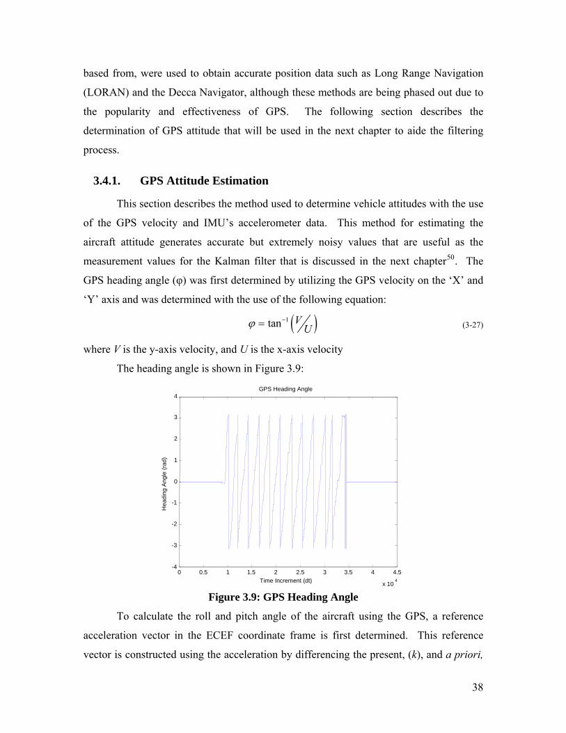
based from, were used to obtain accurate position data such as Long Range Navigation

(LORAN) and the Decca Navigator, although these methods are being phased out due to

the popularity and effectiveness of GPS. The following section describes the

determination of GPS attitude that will be used in the next chapter to aide the filtering

process.

3.4.1. GPS Attitude Estimation

This section describes the method used to determine vehicle attitudes with the use

of the GPS velocity and IMU’s accelerometer data. This method for estimating the

aircraft attitude generates accurate but extremely noisy values that are useful as the

measurement values for the Kalman filter that is discussed in the next chapter50. The

GPS heading angle (φ) was first determined by utilizing the GPS velocity on the ‘X’ and

‘Y’ axis and was determined with the use of the following equation:

( )1tan VUϕ −=

(3-27)

where V is the y-axis velocity, and U is the x-axis velocity

The heading angle is shown in Figure 3.9:

0 0.5 1 1.5 2 2.5 3 3.5 4 4.5 x 10

4 -4

-3

-2

-1

0

1

2

3

4

Time Increment (dt)

Hea

ding

Ang

le (r

ad)

GPS Heading Angle

Figure 3.9: GPS Heading Angle

To calculate the roll and pitch angle of the aircraft using the GPS, a reference

acceleration vector in the ECEF coordinate frame is first determined. This reference

vector is constructed using the acceleration by differencing the present, (k), and a priori,

38

(k-1), values of the GPS velocity. This reference vector represents the aircraft under the

condition that there is no roll or pitch angles. The derivative of the velocity to obtain the

acceleration is then determined by the following:

( ) ( )1GPS GPSGPS

v k v ka v

dt− −

= = (3-28)

where aGPS is the GPS acceleration in ECEF, v is the GPS velocity, and dt is the time

increment.

The GPS acceleration vector is then aligned with the x and y body-axis about the

ECEF z-axis generating the reference acceleration rx and ry. The reference angles are

rotated about the z-axis due to the fact that the reference frame is under the condition that

there is no roll or pitch angles causing the x, y, and z-axes to be orthogonal about the

ECEF z-axis. The rx and ry transformations are defined as:

( ) ( )( )_ _cos sinx GPS x GPS yr a aϕ ϕ= − + (3-29)

( ) ( )( )_ _sin cosy GPS x GPS yr a aϕ ϕ= − − + (3-30)

Since the aircraft is moving in the body frame relative to the ECEF frame, the

IMU’s accelerometers do not feel the effects of gravity. Therefore to compensate the GPS

ECEF acceleration, the reference acceleration is calculated as follows:

_z GPr g a S z= −

( 3-31)

This transformation can be seen graphically in Figure 3.10, where x and y are the

body axis and y’ and x’ is the ECEF axis:

39

Figure 3.10: Rotation about the z-Axis to Align the ECEF Coordinate Frame with

the Body Axis

With the reference vector constructed, the attitudes can then be defined and

calculated with the following set of equations:

2 2

2 2

2x x z x z z

x z

r a r r r ar rθσ

+ + −=

+ (3-32)

1tan z x

z

r ar

θ

θ

σθσ

− ⎛ ⎞−= ⎜ ⎟

⎝ ⎠

(3-33)

( ) ( )sin cosx zr r rθ θ θ= +

(3-34)

2 2 2

2 2

y y y y

y

r a r r r a

r rθ θ

φθ

σ+ + −

=+

(3-35)

1tan Y yr ar

φ

φ θ

σφ

σ−

⎛ ⎞−= ⎜ ⎟⎜ ⎟

⎝ ⎠

(3-36)

Figure 3.11 shows the raw GPS attitude estimate which has a great deal of noise

on in the signal, although it still follows the same trends as the Vertical Gyro data. The

noise from the GPS attitudes is not an issue, for the EKF will compensate for the negative

effects of the noise while still correcting for the drift error associated with the INS.

40

0 100 200 300 400 500 600 700 800 900 -2

-1

0

1

2

Time, tG

PS

Rol

l, ra

d

0 100 200 300 400 500 600 700 800 900 -2

-1

0

1

2

Time, t

GPS

Pitc

h, ra

d

GPS AttitudeVG Attitude

Figure 3.11: GPS vs Vertical Gyro Attitude

To further show that the GPS attitude does actually depict the aircraft roll and

pitch attiude, the noisy values are sent through a low-pass butterworth filter, offline, as

seen in Figure 3.12, then plotted against the vertical gyro data. This representation shows

distinct evidence that this method of estimating the attitude is effective.

0 100 200 300 400 500 600 700 800 900 -2

-1

0

1

Time, t

GP

S R

oll,

rad

0 100 200 300 400 500 600 700 800 900 -2

-1

0

1

2

Time, t

GP

S P

itch,

rad

GPS Attitude

VG Attitude

Figure 3.12: GPS vs Vertical Gyro Attitude

41

3.5. Kalman Filter

The following sections describe the calculations and theory that make up the

Kalman filter. Section 3.5.1 describes the simple Kalman filter, which is only used for

linear systems, while section 3.5.2 discusses the Extended Kalman filter for non-linear

applications.

3.5.1. Introduction to Kalman Filtering

The calculations that make up the filtering process can be separated into two steps

depicted in Figure 3.13; time and measurement update. The time update, or “prediction”

step projects the states and error covariance values ahead in time using the dynamic

model of the system while the measurement update or “correction” step then calculates

the Kalman gain. This value is then used to correct the error in the states and finally

update the error covariance matrix to be input back into the “prediction” equations. The

filtering calculations are discussed in greater detail in the following paragraphs. The

following description is based around the fusion of GPS/IMU data, although a more

general breakdown of the Kalman filter can be seen in greater detail in [5], [40], and [41].

Initial Values for x and P

"Prediction" Equations

1) Project the State Ahead

2) Project the Error Covariance Ahead

"Correction" Equations

1

1 1T T

k k k k k k kK P H H P H R−− −

+ +⎡ ⎤= +⎣ ⎦

1) Compute the Kalman Gain

2) Update Estimate with Measurement z

( )11 1ˆ ˆkk k k k kx x K z H x−+ −

++ += + −

3) Update the Error Covariance

( )1 1k k k kP I K H P+ −+ += −

1T

k k k k kP P Q− ++ = Φ Φ +

1ˆ ˆk k k kx x B u−+ = Φ ⋅ + ⋅

Figure 3.13: Kalman Filter Sequence

42

3.5.1.1. Time Update - “Prediction”

The “prediction” step is composed of two calculations, the predicted state and

covariance calculations, in which the predicted state update is composed of the system

dynamics of the INS, which was discussed in detail in Section 3.3.1. The state update

determines the a priori estimate of the state vector, ‘x,’ at time k, knowing the previous

values for ‘x’ at time k-1.

Step two of the time update section determines the value of the a priori estimate

of the error covariance matrix with the use of the Riccati equation discussed further in the

next section. By utilizing the state transition matrix of the dynamic system (STM, Φ )

and the covariance of the dynamic disturbance (Q), the error covariance matrix, ‘P,’ can

be calculated as follows:

1

Tk k k kP P− +

+ kQ= Φ Φ + (3-37)

The error covariance a priori estimate takes into account that there is a known

error/noise in the input and model of the system which causes the signal to drift or decay

over time from the actual value. Figures of the INS output in Section 3.3.2 are good

examples of the system’s decay over time.

The covariance matrix associated with the dynamic disturbance or model/input

noise, (Qk), estimates the noise that is directly associated with the error in the dynamic

model as well as the noise of the sensor measurement. Equation (3-38) calculates the

estimated value of the model/input covariance matrix, which contributes to the

uncertainty of the dynamic system at each time step.

1 1

Tk k wQ Q 1k− − −= Φ Φ

(3-38)

where Qw is the power spectral density (PSD) of the sensor.

The PSD of the sensor input signals is called white noise due to the fact that it has

the same error at all frequencies as a comparison to the frequency spectrum of white

light. The PSD of the sensor error can be assumed to be zero mean and measured by

conducting a variance analysis on the signal at a steady state response as follows:

( ) ( ) ( ) ( )0, TwE t E t t Q tω ω ω⎡ ⎤= =⎡ ⎤⎣ ⎦ ⎣ ⎦ (3-39)

43

where the first term on the left represents the zero mean random vector of the sensor

input while the second expression represents the PSD analysis of the white noise

associated with the sensor data to generate a matrix associated with each sensor error.

3.5.1.2. Measurement Update – “Correction”

The “correction” step is composed of three calculations; computation of the

Kalman gain, update of the estimated states, and the error covariance a posteriori update.

Computation of the Kalman gain is based on the algebraic (filter) Riccati equation

(ARE)10, which is a discrete recursive equation to calculate the error covariance, P. The

Riccati equation, or the matrix quadratic equation, in its general form is as follows:

( ) 1

1 1 1T T T T

k k k k k k k k k k kP P P H HkP H R H P Q−

+ + +⎡ ⎤= Φ − + Φ +⎢ ⎥⎣ ⎦ k (3-40)

where P is the error covariance matrix, H is the system output matrix, and R is the

covariance matrix of the measurement noise.

By manipulating the Equation (3-38, the a priori covariance matrix, a posteriori

covariance matrix, and the Kalman gain equations are obtained. The a priori calculation

in Section 3.5.1.1 is used to predict an estimate of the error covariance, P, determined

from the system model at the new time step ‘k’ using the a posteriori value from the

previous time step, ‘k-1’.

1

a posterori

Tk k k kP P− +

+ ⎡ ⎤ kQ= Φ Φ +⎣ ⎦

(3-41)

With the a priori estimate of the obtained the Kalman gain can be calculated

which also begins the measurement update portion of the filter. Again referring to the

Riccati equation the Kalman filter gain calculation can be determined as follows:

( )Kalman Gain

1

1 1 1 1 1T T T T

k k k k k k k k k k k kP P P H H P H R H P−+ − − − −

+ + + + +

⎡ ⎤⎢ ⎥= Φ − + Φ +⎢ ⎥⎢ ⎥⎣ ⎦

kQ

(3-42)

( ) 1

1 1T T


+ += + (3-43)

Similar to the system model/input covariance matrix, Qk, the covariance matrix of

the measurement noise is also zero mean white noise (Rk), which is determined as

follows:

44

( ) ( ) ( ) ( )0, TkE v t E v t v t R t⎡ ⎤= =⎡ ⎤⎣ ⎦ ⎣ ⎦

(3-44)

where v is the noise in reference to the measurement data used in the Kalman filter.

The state estimate is next compensated with the use of the Equation (3-45). This

compensation is conducted by first computing the residual between the measurement

(actual) value and the state estimated value. The amount of residual used to correct the

estimated state is determined by multiplying the Kalman gain by the residual.

( )ˆ ˆ ˆk k k k k kx x K z H x+ − −= + − (3-45)

where z is the measurement value.

At this point the a posteriori covariance matrix is calculated by plugging the

Kalman gain back into the Riccati equation to obtain the updated value for the

covariance.

( )a posteriori Covariance Matrix

1

1 1 1 1 1T T T

k k k k k k k k k k k kP P P H H P H R H P Q−+ − − − −

+ + + + +⎡ ⎤= Φ − + Φ +⎢ ⎥⎣ ⎦

k

(3-46)

( )1 1k k kP I K H P+ −+ += −

k (3-47)

This set of calculations is then iterated over the time duration to improve the

states of the system. The Kalman filter’s ability to improve the states can once again be

attributed to the Riccati equation, which is a recursive least squares solution to minimize

the performance index, J, of the system. A good analogy for the performance index can

be referring to it as the “cost” that it takes to put the estimated state back on the optimal

path. As the performance index is minimized the overall accuracy of the system in

improved.

Figure 3.14 depicts the path that the state estimate and covariance matrix take

between two increments in discretized time. As seen from the following figure, the state

transition matrix estimates a new value for the state, ˆkx− , which is then corrected by the

Kalman gain to generate a more accurate value for the state, ˆkx+ .

45

tk tk+1 tk tk+1

kΦ

,k kQΦ

1k+Φ

ˆkx−

ˆkx+

1k−Φ 1ˆkx−+

1ˆkx++

,k kz K

1 1,k kz K+ +

1 1,k kQ− −Φ

1 1,k kQ+ +Φ

kP−

kP+

1kP++

1kP−+

,k kH R1 1,k kH R+ +

a) State Update and Correction b) Covariance Matrix Update andCorrection

Figure 3.14: Kalman Filter Progression of States and Covariance Matrix

The effect of the error covariance has on the system determines the amount of

measurement that gets used to update the state estimates. As the error covariance

decreases, the position of the estimate is trusted more, which doesn’t allow as much of

the measurement to update the estimate. Inversely, if the error covariance increases, the

estimated position is trusted less allowing the measurement position to correct the

estimate. Ideally, as the system progresses over time the value for the error covariance

should get close to zero. This reduction is mainly due to the ‘actual’ measurement values

to maintain the accuracy of the system. Although the model/input noise covariance, Q,

gets added into the error covariance matrix at each time increment limiting the reduction.

3.5.2. Extended Kalman Filter

The Kalman filter is based on the principle that the dynamic model of the system

is linear. Most systems of any level of complexity are composed of non-linear elements,

which draw the need for the extended Kalman filter (EKF). Schmidt introduced the first

application of the EKF during the NASA Ames research discussed earlier. This method

of the Kalman filter has also been referred to as the “Kalman-Schmidt” filter.

It must be noted that by utilizing an EKF increases the level of complexity of the

system by first creating the need to linearize the differential equations and then the update

of the system and input matrix at each time step making the system time variant. These

additional calculations also drastically increase the amount of computational load on the

system.

46

Other than the previous stated criteria, the EKF is relatively similar to the Kalman

filter, as seen in Figure 3.15, the Kalman gain, a priori and a posteriori covariance matrix

calculations are the same as the previous method. An application of the EKF within the

context of this thesis topic is the linearization of the INS attitude determination. The

attitude calculations discussed in Section 3.3.2 involve the use of a time variant linearized

dynamic model that is derived from the non-linear dynamic model seen below.

( )1ˆ ˆk k kx f x w+ −+ = +

(3-48)

( )ˆk kz h x w−k= +

(3-49)

Initial Values for x and P

"Prediction" Equations



"Correction" Equations

1

1 1T T


+ +⎡ ⎤= +⎣ ⎦


2) Update Estimate with Measurement z

( )11 1ˆ ˆkk k k k kx x K z H x−+ −

++ += + −


( )1 1k k k kP I K H P+ −+ += −

1T

k k k k kP P Q− ++ = Φ Φ +

( )1ˆ ˆ ,k k k kx f x u− + ++ =

Update Time Increment (k)

Figure 3.15: Extended Kalman Filter (EKF) Sequence

Referring back to the discussion in section 2.2.2, the extended Kalman filter is not

an optimal filter due to the linearization of the system model. This is described in greater

detail by referring back to the Ricotti equation, in which it is responsible for estimating

and minimizing the error of linear systems. By linearizing the system model by means of

the Taylor series, additional error is induced causing the filter to improperly estimate the

error covariance matrix. The additional error does not pose a great issue, as the EKF is

still a highly effective tool for estimating and reducing the system error. However this

47

does also generate the need for a higher level of accuracy when determining the

covariance matrices, which could cause the filter to diverge if not properly modeled

48

Chapter 4. Experimental Procedures

4.1. Overview of Experimental Procedures

The experimental procedures within the context of this research project required

the development of software algorithms that work with an array of sensor data to meet

the goals and objectives set forth in Section 1.1. This chapter describes the hardware

utilized in the collection of sensor data, the synchronization of the data, and the

implementation of the Kalman filtering methods to achieve the previously stated

objectives. Section 4.2 describes the first phase of this research project in which

previously obtained flight data from the WVU formation flight research was utilized.

4.2. WVU YF-22 IMU/GPS/Vertical Gyro Sensor Fusion

The experimental procedures for this portion of the research project are composed

of a small amount of sensor data manipulation, with the rest being the development of

software algorithms integrating the various sensors to improve the position, velocity and

attitude of the aircraft. Sensor data for this section of the research project was utilized

from the WVU research YF-22 UAV’s during the formation flight research discussed

previously.

The first section, Section 4.2.1, contains the hardware description of the sensors

used for the WVU YF-22 formation flight research project. This flight data is then

utilized in the implementation of the various Kalman filtering software algorithms for the

improvement of the aircraft parameters. The second section, Section 4.2.2 discuses the

limitations of the system and corrective measures taken to achieve results with a higher

level of precision and Section 4.2.3 focuses on the implementation of various Kalman

filtering techniques on the formation flight GPS and IMU data.

4.2.1. Hardware Used for the WVU YF-22 Attitude Improvement

The following section describes the hardware used during the formation flight

research conducted at WVU on three YF-22 test-beds. All data used within the context

of this section was previously recorded flight data, meaning no additional data acquisition

49

was required for this portion of the research topic. This hardware description provides an

insight and background of the YF-22 test vehicles described in Table 4-1.

Table 4-1: WVU YF-22 Test Vehicles/Sensor-Componant Package

Engine Specifications

Value General Vehicle Specifications Value

Engine Type RAM 1000 Maximum Flight Duration (min) 12

Engine hp (hp) 1.9 Maximum Air Speed (km/hr) 213 Fuel Consumption

(oz/min) 12 Take-off Speed (km/hr) 96

RPM (Max) 126,000 Cruising Airspeed (km/hr) 144

Thrust (lbs) 28 Length (m) 2.3 Pressure Ratio 3:1 Wingspan (m) 2

Fuel Type Jet-A Payload (maximum target) (Kg) 5.5 Oil Type Turbine Oil Est. takeoff weight (w/ payload) (Kg) 21

20:1 Est. wing load (with payload) (Kg/m2) 13.7 Fuel/Oil Ratio

3

Est. Thrust/Weight (with payload) 0.6 Fuel Tank Capacity (Kg)

The WVU YF-22 test vehicles were designed, constructed, maintained, and

operated by faculty and students at WVU. The main fuselage is constructed from

fiberglass, while the wings and control surfaces have a foam core, sheeted with balsa

wood, then covered in fiberglass and painted to the three schemes shown in Table 4-1.

The vehicles are powered by RAM 1000 jet engines producing approximately 28 lbs. of

50

thrust allowing the vehicles to achieve a maximum air speed of 213 km/hr (132 mph) and

a cruising velocity of 144 km/hr (89 mph).

The sensor and component package implemented on the formation flight aircraft

in relation to this research consists of an IMU, GPS, Vertical Gyro, and flight computer.

Table 4-2 illustrates the component mounting locations of the IMU, GPS, Vertical Gyro,

flight computer, and power supply, in which each component is discussed in detail

throughout the following sections. Additional sensors and components were

implemented on the aircraft (as presented in Table 4-2), but have no immediate relevance

to this effort.

Table 4-2: Sensor Specifications and Component Mounting

Onboard Sensors Manufacturer Model Number Measurement Type Sampling

Rate

On-Board Computer

(OBC) Microcomputer Systems PC-104

Angular Rates 50 Hz IMU Crossbow IMU400

Linear Accelerations 50 Hz Vertical Gyro Goodrich Sensor Systems VG34 Euler Angles 50 Hz

3-axis Position 20 Hz GPS Novatel OEM4

3-axis Velocity 20 Hz ASCX01DN Differential Pressure 50 Hz Pressure

Sensors SenSym ASCX15AN Absolute Pressure 50 Hz

Angle-of-Attack and Sideslip Vane 50 Hz Nose Probe SpaceAge, Inc. Mini Air Data Boom

Static Dynamic Pressure Taps 50 Hz

51

4.2.1.1. Formation Flight On-Board Computer (OBC)

The OBC, shown in Figure 4.1, was based on a 300 MHz PC-104 stack computer

system, which contained a CPU module, a data acquisition module, a power supply

module, and supporting components. The PC-104 format was selected because of its

reduced size, lightweight, and low power consumption2.

ControllerBoard

DAQ Card

CPU Card

CF Card Reader

Power SupplyCard

Servo ControlModule

Interface-Board

Computer Box

ControllerBoard

DAQ Card

CPU Card

CF Card Reader

Power SupplyCard

Servo ControlModule

Interface-Board

Computer Box

Figure 4.1: YF-22 Onboard Computer2

4.2.1.2. NovAtel GPS Receiver

A NovAtel OEM4 GPS receiver was used to measure the 3-axis position and

velocity to meter level accuracy, which was read into the flight computer at a rate of 20

Hz. This data was required for each of the three YF-22 test-beds in order to achieve

formation flight, in which position and distance information between the aircraft had to

be obtained. While the flight computer recorded only the position and velocity

information, the OEM4 receiver is capable of obtaining a variety of additional

information depending on the firmware configuration purchased through NovAtel,

including the ability to obtain raw pseudorange and ephemeral data, along with real-time

kinematic (RTK) processing which allows the receiver to obtain position data at a level of

either 2 or 20 cm accuracy.

52

(a) NavAtel GPS Receiver (b) GPS Antenna Location

Figure 4.2: NovAtel GPS

The selected GPS antenna was the GPS-511, also manufactured by Novatel, Inc.,

which offered desirable performance for airborne and high dynamic applications.

The GPS antenna was mounted on the top section of the aircraft fuselage at the center of

gravity (CG) location, as shown in Figure 4.2 (b), in relation to the IMU, Vertical Gyro,

and power supply.

4.2.1.3. Crossbow IMU

The Crossbow IMU400CC-200 was selected for the formation flight research due

to its lightweight, cost, and performance abilities. This component was a solid-state 6-

degree-of-freedom (6 DOF) inertial package intended for navigation and control,

dynamic testing, and instrumentation applications. This system provided measurements

of the angular rates and linear accelerations along three orthogonal axes. Fully

compensated angular rate and acceleration outputs were provided in both analog and

digital (RS-232) formats, which were recorded at a rate of 50 Hz by the flight computer.

53

Table 4-3: Crossbow IMU400CC-200 Specifications

Performance Maximum Update Rate (Hz) 100

Range: Roll, Pitch, Yaw (°/sec) 200± Angular Rate

Bias: Roll, Pitch, Yaw (°/sec) 1< ±

Range: X, Y, Z (g) 10± Acceleration

Bias: X, Y, Z (mg) 12< ±

4.2.1.4. Goodrich Sensor Systems Vertical Gyro

The vertical gyro attitudes were obtained by a Goodrich Sensor Systems brand,

model VG34 vertical gyro, shown in Figure 4.3. This unit is Goodrich Sensor System’s

smallest vertical gyro, that produces highly accurate measurements in which the range is

±90° for the roll angle, with an accuracy of ±1°, and ±60° for the pitch angle, also with an

accuracy of ±1°.

Figure 4.3: Goodrich Systems Vertical Gyro

The size, cost, and accuracy of the VG34 make it a an optimal choice for many

additional high performance vehicles such as tracked wheeled and tracked armored

vehicles, aircraft, helicopters, missiles, drones and remotely piloted aerial vehicles

54

4.2.2. Limitations/Corrections to the WVU Formation Flight Hardware

Setup

Although the data collected during the formation flight research project was

actual flight data, which in many ways increases the validity of the data and results, also

creates some limitations on the project at hand. Along with some of the limitations and

restrictions of the collected data, there are also some additional corrective measures that

have been conducted.

GPS Position Data

The GPS data collected during flight tests consisted of only position and velocity

data, no pseudorange, or raw ephemeral data was collected. This restricts the Kalman

filter to a loosely coupled system, which will be discussed in greater detail later in this

chapter.

Acquisition Rate

The first issue between the IMU and GPS data being utilized is the difference in

the sampling rates. The IMU samples were taken at 50 Hz while the GPS samples could

be obtained at 20 Hz, which causes the data to only match on increments of 0.1 s. The

optimal method for utilizing most of the flight data was to resample the IMU sensor

information at 40 Hz and maintain the GPS data at 20 Hz. This allowed the Kalman Filter

to correct for the IMU’s data every other time step instead of every fifth time step, as

seen in Figure 4.4.

Figure 4.4: IMU vs. GPS Measurement Acquisition Rate

Lever Arm Correction

The lever arm correction compensates for the offset distance between the GPS

antenna and the IMU sensor, which realigns the position and velocity data between the

55

two sensors - back to the CG of the aircraft. This offset is caused by three main factors; a)

the sensors cannot overlap each other, b) the GPS antenna must be placed on the fuselage

of the aircraft, and c) to properly balance the aircraft the, sensors must be strategically

placed within the aircraft. This correction was conducted by adjusting the relative

acceleration for one point (the IMU), rotating about a second point (the GPS antenna, at

the CG location). The lever arm correction was conducted with the use of the following40:

2a a rBA α ω= − ⋅ + ⋅ d

2 2002 20 0

2 20 0

r qa a r dr q

(4-1)

x x x xa a r dy y r p y r p ya a r dz z z zq pA B q p

ω ωα α

α α ω ω

α α ω ω

⎡ ⎤−⎡ ⎤−⎡ ⎤ ⎡ ⎤ ⎡ ⎤ ⎡ ⎤⎢ ⎥⎢ ⎥⎢ ⎥ ⎢ ⎥ ⎢ ⎥ ⎢ ⎥⎢ ⎥= − − + −⎢ ⎥⎢ ⎥ ⎢ ⎥ ⎢ ⎥ ⎢ ⎥⎢ ⎥⎢ ⎥⎢ ⎥ ⎢ ⎥ ⎢ ⎥ ⎢ ⎥⎢ ⎥−⎢ ⎥⎣ ⎦ ⎣ ⎦ ⎣ ⎦ ⎣ ⎦−⎣ ⎦ ⎢ ⎥⎣ ⎦

(4-2)

where α is the angular acceleration, ω is the angular rate, and r is the position offset from

the GPS antenna location to the IMU location.

The angular acceleration was then determined by differencing the angular rate

from the time step k, with the previous time step k-1. The values for the angular velocities

and accelerations are then placed into a skew matrix so that each directional component

of the acceleration will be corrected.

Bad Measurement Determination

Bad measurements from degraded GPS signal data were also accounted for when

analyzing flight data. The main periods for when the GPS data precision deteriorated

during the WVU formation flight test experiments was during high bank angle

maneuvers, as depicted in Figure 4.5, although while testing the validation data there was

one instance when a total signal loss was discovered as seen in Figure 4.6.

56

822 824 826 828 830 832 834 836 838 840

410

415

420

425

430

435

440

445

450

455

460

Nor

th C

ompo

nent

, m

East Component, m

GPS

Figure 4.5: GPS Position (Magnified)

0 100 200 300 400 500 600 700 800 900-2.5

-2

-1.5

-1

-0.5

0

0.5x 10236

East Component, m

Nor

th C

ompo

nent

, m

GPS

Figure 4.6: GPS Position - Instantaneous Signal

Loss

While the filtering process compensated for the GPS error, the elimination of

measurements that were unrealistic produced higher quality and more accurate results.

Since the vehicles main dynamic movement is along the longitudinal axis, a significant

lateral maneuver was unrealistic and not probable. Therefore whenever this type of

movement was detected, the measurement was neglected and only the INS measurement

utilized. Although the INS system is susceptible to drift effects, the short-term use of only

the INS values is more precise than the filtered estimates.

This correction was accomplished by comparing the Kalman filter residual

calculation, ( 1ˆi i i )z H x −− , at time ‘k’ with the standard deviation. When the value of the

residual exceeds a set threshold value of the standard deviation, the GPS value for that

given time increment is omitted and the IMU’s dynamic model computes the transition to

the next increment.

4.2.3. Software Used for the Integration of GPS/INS

Within the context of creating Kalman filtering algorithms for the fusion of the

YF-22 formation flight data, four methods were implemented, in which each method has

benefits and drawbacks to be further discussed throughout this section.

57

4.2.3.1. Fusion of IMU/GPS/Vertical Gyro data

This method fuses the GPS position and velocity, INS position and velocity, and

the Vertical Gyro attitudes. The fusion of this method uses the GPS and INS components

of position and velocity as the states within the Kalman filter, in which the benefit of this

is to remove the drift within the INS and the signal errors in the GPS components of the

position and velocity. The attitudes from the Vertical Gyro are used so that there is no

need for non-linear modeling, allowing the use of the Kalman filter.

The algorithm for implementing the first method is composed of three main

functions:

1) Data Preprocessing

2) INS Calculations

3) Kalman Filter Implementation

The data preprocessing is composed of the acquisition rate correction (discussed in the

previous section) and the initialization of the filtering parameters.

The initialization of the filter is composed of the initial values of the state vector

and error covariance matrix as well as the setting up of the system model/input and

measurement noise covariance matrices, Q and R respectively. Initially the 6x6 error

covariance matrix, P, was set to zeros since the exact initial position was known and the

initial state vector, 0x̂ , was also set to zeros in which both parameters got updated after

each filtering iteration.

The measurement noise covariance matrix was determined by obtaining the

variance of the GPS position and velocity measurements over a steady state period of

time. Figure 4.7 depicts an example of the period in which the variance was obtained.

58

Figure 4.7: Steady State Time Period for Variance Calculation

These values were then inserted into a diagonal matrix respectively to generate the

measurement noise covariance matrix of the GPS data: 2

2

2

2

2

2

-4

-4

-4

0 0 0 0 0

0 0 0 0 0

0 0 0 0 0

0 0 0 0 0

0 0 0 0 0

0 0 0 0 0

0.0022 0 0 0 0 00 0.0017 0 0 0 00 0 0.0046 0 0 00 0 0 2.0988e 0 00 0 0 0 1.7912e 00 0 0 0 0 5.3837e

North

East

Down

North

East

Down

x

y

z

u

v

w

R

σ

σ

σ

σ

σ

σ

⎡ ⎤⎢ ⎥⎢ ⎥⎢ ⎥⎢ ⎥= =⎢ ⎥⎢ ⎥⎢ ⎥⎢ ⎥⎢ ⎥⎣ ⎦

⎡ ⎤⎢ ⎥⎢ ⎥⎢ ⎥⎢ ⎥⎢ ⎥⎢ ⎥⎢ ⎥⎣ ⎦

As discussed previously in this chapter, the filtering approach was restricted to a

‘loosely’ coupled system due to the lack of raw GPS data. A ‘loosely’ coupled system,

although easier to implement than a tightly coupled system, does not estimate the IMU

calibration parameters (e.g. biases), leaving the estimation of these parameters to the

system designer.

These IMU calibration parameters were set into the model/input covariance

matrix, Q, and are used as a tuning parameter. If the system designer did not correctly

59

estimate these parameters, a reduction in the performance of the filter could occur6. This

is not the case for ‘tightly’ coupled systems, in which these values are properly modeled

as discussed in Section 3.5.1.1.

As a starting point for the initialization of the model/input covariance matrix, any

value could be selected so that the value is greater than zero, but less than one; to obtain

starting values, the initial values for this method were determined the same way as the

measurement covariance matrix by placing the IMU acceleration variance during a

steady-state condition in a 6x6 diagonal matrix for the position and velocity as seen

below:

3 3 1 3 1 3 1 3 3 3 1 3 1 3 1 32

3 1 3 12

3 1 3 12

3 13 1

0 0 0 0 0 0 0 00 0 0 0 .004 0 00 0 0 0 0 .0037 0

0 0 0 .00460 0 0

x

y

z

x x x x x x x x

x a x

x a x

xx a

Qσ

σ

σ

⎡ ⎤ ⎡ ⎤⎢ ⎥ ⎢ ⎥⎢ ⎥ ⎢ ⎥= =⎢ ⎥ ⎢ ⎥⎢ ⎥ ⎢ ⎥⎢ ⎥ ⎣ ⎦⎣ ⎦

The location for the position covariance values are intentionally left zero since they are a

direct integration from the velocity, which values in the covariance matrix are composed

of the variance of the acceleration data. The error associated with the velocity from the

integration of the accelerometer and gyroscope data is directly passed on to the position.

Meaning that by reducing the error in the velocity integration, the error in the position

also decreases.

From these values if the model/system covariance were increased so that the value

was closer to one, the system would closer mimic the measured value. Inversely, as the

covariance approaches zero, the system would closer mimic the estimated values. After

the initial system has been established these values are adjusted to suit the needs of the

system. This tuning is explained and discussed further in the next chapter.

The INS calculations, with the exception of the integration of the attitudes, are

discussed in detail in section 3.3.1. Again, the integration of the attitudes was neglected

for this method since the vertical gyros attitude values were used. This allows the INS

calculations to begin at equation (3-24) with the DCM being calculated using the vertical

gyro’s attitudes.

60

With the data preprocessing and initialization complete, the Kalman filter can be

implemented to improve the position and velocity data. Figure 4.8 illustrates a block

diagram of the data flow throughout the filter resulting in the corrected data.

Gyroscope

Accelerometer

IMU

(ax, ay, az)body



(DCM)

(axayaz)nav

φ θ ψ

Position/Velocity

Integration Position,Velocity

Position,Velocity

pv

δδ

Vertical Gyro

GPS Nav FilterPosition, Velocity

φ θ ψ

Figure 4.8: Block Diagram of a GPS Aided INS/Vertical Gyro

With the INS calculations, GPS, and vertical gyro data already discussed, the

focus shifts to combining the data from the three sources in the proper manner so that the

filter is implemented correctly. With the initial values set, the “prediction” step of the

Kalman filtering process can be conducted in which the a priori covariance matrix and

new state estimates are obtained. Revisiting Figure 3.13 and tailoring these equations to

this specific application; Table 4-4 is constructed which distinctly defines each

expression in the filtering process.

Table 4-4: "Prediction" Equations (Method I) Nomenclature Symbol Matrix

Size Values


1ˆ ˆk k k kx x B u−+ = Φ ⋅ + ⋅ System States 1ˆ ˆ,k kx x−

+ 6x1 ,3 1

,3 1

k x

k x

xv

⎡ ⎤⎢ ⎥⎣ ⎦

61

STM kΦ 6x6 3 3 3 3

3 3 3 30x x

x x

I I dtI

⋅⎡ ⎤⎢ ⎥⎣ ⎦

Input Matrix B 6x3 3 3

3 3

0 x

xI dt⎡ ⎤⎢ ⎥⋅⎣ ⎦

Inputs ku 3x1 3 1navxa⎡ ⎤⎣ ⎦

STM kΦ 6x6 3 3 3 3

3 3 3 30x x

x x

I I dtI

⋅⎡ ⎤⎢ ⎥⎣ ⎦

Model/Input Covariance

Matrix kQ 6x6

2,3 3

2,3 3

( ) 03 30 (3 3

r x

v x

diag xdiagx

σ

σ )

⎡ ⎤⎢ ⎥⎢ ⎥⎢ ⎥⎣ ⎦


1T

k k k kP P− ++ = Φ Φ + kQ

Error Covariance

Matrix 1,k kP P− +

+ 6x6 ( )6 6xdiag X⎡ ⎤⎣ ⎦

At this point the “correction” step was calculated in which the Kalman gain, Eq.

(3-43), state corrections, Eq. (3-45), and a posteriori covariance matrix, Eq. (3-47), were

calculated. Table 4-5 was constructed which distinctly defines each expression

“Correction” portion of the filtering process.

Table 4-5: "Correction" Equations (Method I) Nomenclature Symbol Matrix

Size Values

Error Covariance

Matrix 1kP−

+ 6x6 ( )6 6xdiag X⎡ ⎤⎣ ⎦

Measurement Covariance

Matrix kR 6x6

2,3 3

2,3 3

( ) 03 30 (3 3

r x

v x

diag xdiagx

σ

σ )

⎡ ⎤⎢ ⎥⎢ ⎥⎢ ⎥⎣ ⎦

Kalman Gain kK 6x6 ( )6 6xdiag X⎡ ⎤⎣ ⎦

1) Compute the Kalman Gain 1

1 1T T


+ +⎡ ⎤= +⎣ ⎦

Observation Matrix kH 6x6 3 3 3 3

3 3 3 3

00

x x

x x

II

⎡ ⎤⎢ ⎥⎣ ⎦

System States 1ˆ ˆ,k kx x−+ 6x1

,3 1

,3 1

k x

k x

xv

⎡ ⎤⎢ ⎥⎣ ⎦

GPS ent Measurem

Value kz 6x1

,3 1

,3 1

k x

k x

xv

⎡ ⎤⎢ ⎥⎣ ⎦

2) Update Estimate with Measurement “z”

( )ˆ ˆkk k k k kx x K z H x− −= + −


3 3 3 3

00

x x

x x

II

⎡ ⎤⎢ ⎥⎣ ⎦

3) Update the Error Covariance: ( )1 6 6k x k kP I K H P+

+ += − 1k−

Error Covariance


+ 6x6 ( )6 6xdiag X⎡ ⎤⎣ ⎦

62

Kalman Gain kK 6x6 [ ]6 6xX


3 3 3 3

00

x x

x x

II

⎡ ⎤⎢ ⎥⎣ ⎦

Further describing the previous table, the state correction contains the observation

vector (z), predicted observation vector ( ˆk kH x− ), and the Kalman gain matrix (K). The

observation vector was a 6x1 matrix that is composed of the GPS values for position and

velocity while the 6x1 predicted observation vector was composed of the INS values for

the position and velocity. The observation vector and predicted observation vector were

then differenced to make up the residual in Eq. (3-45), which then gets multiplied by the

Kalman gain and summed with the state estimate to produce the filtered results. The

updated state vector was then fed back into the INS computation to predict the next

increment.

At this point, all of the parameters, inputs, and expressions needed for the filtering

process have been well defined and the simulation was coded in Matlab®. As described

in section 4.2.2, the IMU and GPS data is obtained at 40 and 20 Hz respectively, meaning

that filtering will occur every other reading obtained from the IMU, which is illustrated

graphically in Figure 4.9.

63

IMU/VG Kalman Filter IMU/VGPositionVelocity

PositionVelocity

PositionVelocity

GPS

Pos

ition

Vel

ocity

acceleration, k

acce

lera

tion,

k+1

Figure 4.9: Filter Process Sequence

4.2.3.2. Fusion of IMU/GPS Data Using GPS Attitude Estimates

This second method fuses the GPS position and velocity/GPS estimated attitudes

with the INS position, velocity, and attitude. There are two main differences from the

previous method, which now entail the calculation of the non-linear kinematic equations

to determine the aircraft attitude, which also forces the need for the EKF and the

estimation of the GPS attitudes discussed in Section 3.4. This is the first implementation

in which the vertical gyro is eliminated and the navigation system relies solely on the

extended Kalman filter to correct for the attitude drift.

In addition to the first two functions conducted in the first method, this second method

also entails:

1) Data Preprocessing (From Method I)

2) INS Calculations (From Method I)

3) Attitude Integration and Linearization

4) GPS Attitude Estimation

5) Extended Kalman Filter Implementation.

Most of the data preprocessing and parameter initialization remains consistent from the

first method; the major differences for the implementation are the addition of the

nonlinear calculations of the attitudes in the EKF, the estimation of the model/input

64

covariance matrix (Q), and the addition of the GPS attitude variance values to the

measurement covariance matrix which is depicted graphically in Figure 4.10.

Gyroscope

Accelerometer

IMU

(ax, ay, az)body



(DCM)

(axayaz)nav

φ θ ϕ

GPS

PositionVelocity

PositionVelocity

pv

δδ

Position/Velocity

Integration

PositionVelocity

GPS AttitudeCalculation

Kalman Filter

δΨ

Figure 4.10: Block Diagram for the GPS Aided INS System

With the addition of the GPS attitude in the observation vector, z, the measurement

covariance matrix, R, gets expanded from the 6x6 diagonal matrix composed of the

position and velocity covariance to a 9x9 diagonal matrix composed of the position,

velocity, and attitude. 2

2

2

2

2

2

2

2

2

0 0 0 0 0 0 0 0

0 0 0 0 0 0 0 0

0 0 0 0 0 0 0 0

0 0 0 0 0 0 0 0

0 0 0 0 0 0 0 0

0 0 0 0 0 0 0 0

0 0 0 0 0 0 0 00 0 0 0 0 0 0 00 0 0 0 0 0 0 0

North

East

Down

North

East

Down

x

y

z

u

v

w

R

φ

θ

ϕ

σ

σ

σ

σ

σ

σ

σσ

σ

⎡ ⎤⎢ ⎥⎢ ⎥⎢ ⎥⎢ ⎥⎢ ⎥⎢ ⎥

= =⎢ ⎥⎢ ⎥⎢ ⎥⎢ ⎥⎢ ⎥⎢ ⎥⎢ ⎥⎢ ⎥⎣ ⎦

65

-4

-4

-4

0.0022 0 0 0 0 0 0 0 00 0.0017 0 0 0 0 0 0 00 0 0.0046 0 0 0 0 0 00 0 0 2.0988e 0 0 0 0 00 0 0 0 2.0988e 0 0 0 00 0 0 0 0 5.3837e 0 0 00 0 0 0 0 0 0.0019 0 00 0 0 0 0 0 0 0.0023 00 0 0 0 0 0 0 0

⎡ ⎤⎢ ⎥⎢ ⎥⎢ ⎥⎢ ⎥⎢ ⎥⎢ ⎥⎢ ⎥⎢ ⎥⎢ ⎥⎢ ⎥⎢ ⎥⎢ ⎥⎣ ⎦0

The process for estimating the model/input covariance matrix was conducted the

same way as to determine the values for measurement covariance matrix. For the

model/input covariance matrix, the variance of the IMU raw accelerometer and angular

rate data is used for the diagonal as seen below:

3 3 1 3 1 3 1 3 1 3 1 3 1 3 3 3 1 3 1 3 1 3 1 3 1 3 1 32

3 1 3 12

3 1 3 12

3 13 1

23 1

23 1

23 1

0 0 0 0 0 0 0 0 0 0 0 0 0 00 0 0 0 0 0 0 .004 0 0 0 0 00 0 0 0 0 0 0 0 .0037 0 0 0 0

0 0 0 .0046 0 0 00 0 0 0 0 000 0 0 0 0 0

0 0 0 0 0 00 0 0 0 0 0

x

y

z

x x x x x x x x x x x x x x

x a x

x a x

xx a

x p

x q

x r

Q

σ

σ

σ

σσ

σ

⎡ ⎤⎢ ⎥⎢ ⎥⎢ ⎥⎢ ⎥

= =⎢ ⎥⎢ ⎥⎢ ⎥⎢ ⎥⎢ ⎥⎢ ⎥⎣ ⎦

-83 1

-83 1

-83 1

0 0 0 1.843e 0 00 0 0 0 0 1.289e 00 0 0 0 0 0 1.293e

x

x

x

⎡ ⎤⎢ ⎥⎢ ⎥⎢ ⎥⎢ ⎥⎢ ⎥⎢ ⎥⎢ ⎥⎢ ⎥⎢ ⎥⎣ ⎦

The addition of the INS attitude creates two major changes to the software

algorithm; first, to project the state ahead, the nonlinear aircraft kinematic equations are

used, while secondly, the aircraft kinematic equation’s Jacobian matrix of partial

derivates from Equation (3-19) is inserted into the state transition matrix for use in the

calculation of the a priori error covariance matrix. Table 4-6 shows the “Prediction”

calculations used for this method in which the determination of the state vector and

Jacobian matrix was discussed in detail in Section 3.3.2.

66

Table 4-6: "Prediction" Equations (Method II)


3 1, 1 3 3 3 3 3 33 1

3 1, 1 3 3 3 3 3 3

00

x k x x k x navx

x k x x k x

x I I dt xa

v I v I dt+

+

⋅⎡ ⎤ ⎡ ⎤ ⎡ ⎤ ⎡ ⎤⎡ ⎤= ⋅ +⎢ ⎥ ⎢ ⎥ ⎢ ⎥ ⎢ ⎥ ⋅ ⎣ ⎦⋅⎣ ⎦ ⎣ ⎦ ⎣ ⎦⎣ ⎦

( )1= p +q sin( ) tan( )+r cos( ) tan( )k k k k k k k k k dtφ φ φ θ φ θ+ + ⋅ ⋅ ⋅ ⋅ ⋅


( )( )1 1= sin( )+r cos( ) sec( )k k k k k k kq dtψ ψ φ φ θ+ + + ⋅ ⋅ ⋅ ⋅

3 1, 1 3 1, 1 1 1 1[ , , , ,k x k x k k k kx x v φ θ ϕ−

]+ + + + +=

Nomenclature Symbol Matrix Size Values

STM kΦ 9x9 3 3 3 3 3 3

3 3 3 3 3 3

3 3 3 3 ,3 3

00 00 0

x x x

x x x

x x

I I dtI

JΨ

⎡ ⎤⋅⎢ ⎥⎢ ⎥⎢ ⎥⎣ ⎦x


Matrix kQ 9x9

3 3 3 3 3 32

3 3 ,3 3 3 32

3 3 3 3 ,3 3

0 0 0

0 ( ) 0

0 0 (

x x x

x v x x

x x x

diag

diag ψ

σ

σ

⎡ ⎤⎢ ⎥⎢ ⎥⎢ ⎥⎢ ⎥⎣ ⎦


)

1T


Error Covariance


+ 9x9 ( )6 6 6 3

3 3 3 3

00

x x

x x

diag XX

⎡ ⎤⎢ ⎥⎣ ⎦

The resulting “Correction” calculations seen in Table 4-7 are similar to that of the

previous method with the exception that the GPS attitude was added to the GPS

observation vector, z, and the change in the size of each matrix to accommodate the

additional three components of the attitude. The new observation vector was a 9x1

matrix that is composed of the GPS values for position, velocity, and attitude while the

9x1 predicted observation vector was composed of the INS values for the position,

velocity, and attitude. The following table shows the “Correction” calculations including

a detailed description.

Table 4-7: "Correction" Equations (Method II) Nomenclature Symbol Matrix

Size Values

1) Compute the Kalman Gain Observation Matrix kH 9x9 [ ]9 9xI

67

Error Covariance

Matrix 1kP−

+ 9x9 ( )6 6 6 3

3 3 3 3

00

x x

x x

diag XX

⎡ ⎤⎢ ⎥⎣ ⎦


Matrix kR 9x9

2,3 3

2,3 3

2,3 3

( ) 0 03 3 3 30 ( ) 03 3 3 30 0 (3 3 3 3

r x

v x

x

diag x xdiagx x

diagx x

σ

σ

σ Ψ

1

1 1T T


+ +⎡ ⎤= +⎣ ⎦

)

⎡ ⎤⎢ ⎥⎢ ⎥⎢ ⎥⎢ ⎥⎢ ⎥⎣ ⎦


System States 1ˆ ˆ,k kx x−+ 9x1

,3 1

,3 1

,3 1

k x

k x

k x

xv

⎡ ⎤⎢ ⎥⎢ ⎥⎢ ⎥Ψ⎣ ⎦

GPS Observation

Vector kz 9x1

,3 1

,3 1

,3 1

k x

k x

k x

xv

⎡ ⎤⎢ ⎥⎢ ⎥⎢ ⎥Ψ⎣ ⎦

Observation Matrix kH 9x9 [ ]9 9xI



Error Covariance


+ 9x9 ( )6 6 6 3

3 3 3 3

00

x x

x x

diag XX

⎡ ⎤⎢ ⎥⎣ ⎦


Observation Matrix kH 9x9 [ ]9 9xI 3) Update the Error Covariance

( )1 6 6k x k kP I K H P+ −+ += − 1k Error

Covariance Matrix

1kP−+ 9x9

( )6 6 6 3

3 3 3 3

00

x x

x x

diag XX

⎡ ⎤⎢ ⎥⎣ ⎦



in the previous section, the IMU and GPS data was again obtained at 40 and 20 Hz

respectively, meaning that the filtering occurred every other measurement obtained from

the IMU.

4.2.3.3. Fusion of IMU/GPS data

The third method directly corrects the position and velocity within the Kalman

filter algorithm, and indirectly corrects the attitudes since they directly map to the

position and velocity through the direction cosine matrix. This method compensates for

the Euler angle errors by incorporating the DCM into the system matrix instead of

converting the acceleration to the local axis prior to the filtering process, which is the

only link between the GPS data and the IMU angular rate data. Without having the DCM

68

in the system matrix or a measurement value for the residual, no compensation can occur

within the filter. With this said, the third method required the following changes to be

made in the formulation of the simulation algorithm:

1. Data Preprocessing (From Method I & II)

2. INS Calculations (From Method II)

3. Attitude Integration and Linearization (From Method II)

4. DCM Linearization

5. Extended Kalman Filter Implementation

Elements from the data preprocessing and parameter initialization remain consistent from

the first two methods, although with the removal of the GPS attitude estimates, the

measurement covariance matrix, R, resort back to the matrix used in method I, while the

system/input covariance matrix, Q, is the same as method II.

Gyroscope

Accelerometer

IMU

(ax, ay, az)body



(DCM)

(axayaz)nav

φ θ ϕ

Position/Velocity

Integration

GPS Kalman FilterPosition, Velocity

PositionVelocity

PositionVelocity

pv

δδ

δΨ

Figure 4.11: Block Diagram for the GPS/INS System (Method III)

To further elaborate on the introduction, if the STM is only made up of the

position, velocity, and kinematic equations, the error covariance matrix will take on the

form depicted at point A in Figure 4.12 below. This value is then input into the Kalman

69

gain calculation in which the gain turns out to be a 9x6 matrix with the bottom three rows

being zeros, as seen at point B. These bottom three rows of the gain matrix make up the

gain associated with the attitude, causing there to be no correction to the estimated

attitude states, resulting in the final output at point C. (NOTE: Positions within Figure

4.12 containing the character ‘X’ represent any real number.)

E

A

B

( )

[ ]( )3 3 3 3 3 3

13 3 3 3 3 3 6 6 6 3 6 6

3 3 3 3 3 3

0 00 0 00 0

1 6 61 1

3 30

x x x

x x x x x x

x x x

II I X

X

xT Tk k k k k k k

x

XK P H H P H R

−⎡ ⎤⎢ ⎥⎢ ⎥⎢ ⎥⎣ ⎦

−− −+ +

⎡ ⎤= + = ⎢ ⎥

⎣ ⎦

( )6 6 3 1 3 1

3 3 3 1 3 1

3 1

3 1

3 10

ˆ ˆ ˆ

x x x

x x vxGPS INS

x

k k k k k k x

X r r xv v

rx x K z H x v+ − −

⎛ ⎞⎡ ⎤ ⎡ ⎤ ⎡ ⎤−⎜ ⎟⎢ ⎥ ⎢ ⎥ ⎢ ⎥⎜ ⎟⎣ ⎦ ⎣ ⎦ ⎣ ⎦⎝ ⎠

⎡ ⎤⎢ ⎥= + − = ⎢ ⎥⎢ ⎥Ψ⎣ ⎦

[ ]3 3 3 3 3 3 3 3 3 3 3 3 3 3 3 3 3 3

3 3 3 3 3 3 9 9 3 3 3 3 3 3 3 3 3 3 3 3

3 3 3 3 ,3 3 3 3 3 3 ,3 3 3 3 3 3 3 3

0 0 0 0 0 00 0 0 0 0 00 0 0 0 0 0

Tx x x x x x x x x

x x x x x x x k x x x

x x x x x x x x x

I I II I I Q I

J J X

T P Qk k k k

Ψ Ψ

⎡ ⎤ ⎡ ⎤ ⎡ ⎤⎢ ⎥ ⎢ ⎥ ⎢ ⎥+ =⎢ ⎥ ⎢ ⎥ ⎢ ⎥⎢ ⎥ ⎢ ⎥ ⎢ ⎥⎣ ⎦⎣ ⎦ ⎣ ⎦

+Φ Φ +⎡ ⎤⎣ ⎦1kP−+ =

C

D

Figure 4.12: Kalman Process Diagram

With further inspection of Figure 4.12, to be able to obtain a gain within the

bottom three rows at B, it is obvious that there are only two options. The first is to have

an additional measurement value (e.g. GPS attitude estimate as used for the previous

section) so that the observation matrix, (H, point D), becomes a 9x9 matrix, allowing the

Kalman gain to correct for all of the states.

The second option is to generate nonzero values for the first two rows of the third

column in the state transition matrix, which would then allow nonzero values to be

obtained in the error covariance matrix (point E). This is achieved by placing the DCM

directly into the second row, third column of the STM so that the error associated with

the rotation from the body axis to the local tangent frame can be estimated by the gain.

Since the calculation of the DCM is nonlinear, a Taylor series approximation is now

required for the velocity states in a similar fashion to the linearization of the aircraft

70

kinematic equations. Only the Jacobian approximation for the system matrix is displayed

due to the fact that the linearized input matrix is not utilized in the filtering process. Also

keep in mind that the error associated with the hot’s is neglected.

( ), ,

f f f

f f fJ

f f f

δ θ δ φ δ ϕ

δφ δθ δϕ

δ θ δ φ δ ϕφ θ ϕ

δφ δθ δϕ

δ θ δ φ δ ϕ

δφ δθ δϕ

⎡ ⎤⎛ ⎞ ⎛ ⎞ ⎛ ⎞⎜ ⎟ ⎜ ⎟ ⎜ ⎟⎢ ⎥⎝ ⎠ ⎝ ⎠ ⎝ ⎠⎢ ⎥

⎢ ⎥⎢ ⎥⎛ ⎞ ⎛ ⎞ ⎛ ⎞⎢ ⎥⎜ ⎟ ⎜ ⎟ ⎜ ⎟

⎝ ⎠ ⎝ ⎠ ⎝ ⎠⎢ ⎥= =⎢ ⎥⎢ ⎥

⎛ ⎞ ⎛ ⎞ ⎛ ⎞⎢ ⎥⎜ ⎟ ⎜ ⎟ ⎜ ⎟⎢ ⎥⎝ ⎠ ⎝ ⎠ ⎝ ⎠

⎢ ⎥⎢ ⎥⎢ ⎥⎣ ⎦

i i i

i i i

i i i

( ) ( ) (

2 2q cos ( ) tan( )-r sin ( ) tan( ) sin( ) sec ( )+r cos( ) sec ( ) 0sin ( )-r cos ( ) 0 0

cos ( )-r sin ( ) sec( ) sin( )+r cos( ) sec( ) tan 0

qq

q q

φ θ φ θ φ θ φ θφ φ

φ φ θ φ φ θ θ

⎡ ⎤⋅ ⋅ ⋅ ⋅ ⋅ ⋅ ⋅ ⋅⎢ ⎥− ⋅ ⋅⎢ ⎥⎢ ⎥⋅ ⋅ ⋅ ⋅ ⋅ ⋅ ⋅⎣ ⎦)

(4-3)

After substituting the DCM Jacobian matrix into the state transition matrix the

error covariance matrix takes in the form seen at point A in Figure 4.13. This in turn

allows for the attitude error to be estimated in the bottom three rows of the Kalman gain

as seen at point B.

A

B

( )

[ ]( )3 3 3 3 3 3

13 3 3 3 3 3 6 6 6 3 6 6

3 3 3 3 3 3

0 00 00 0

1 6 61 1

3 3

x x x

x x x x x x

x x x

II X I X

X

xT Tk k k k k k k

x

XK P H H P H R

X

−⎡ ⎤⎢ ⎥⎢ ⎥⎢ ⎥⎣ ⎦

−− −+ +

⎡ ⎤= + = ⎢ ⎥

⎣ ⎦

( )6 6 3 1 3 1

3 3 3 1 3 1

3 1

3 1

3 1

ˆ ˆ ˆ

x x x

x x vxGPS INS

x

k k k k k k x

X r r xX v v

rx x K z H x v+ − −

⎛ ⎞⎡ ⎤ ⎡ ⎤ ⎡ ⎤−⎜ ⎟⎢ ⎥ ⎢ ⎥ ⎢ ⎥⎜ ⎟⎣ ⎦ ⎣ ⎦ ⎣ ⎦⎝ ⎠

⎡ ⎤⎢ ⎥= + − = ⎢ ⎥⎢ ⎥Ψ⎣ ⎦

[ ]3 3 3 3 3 3 3 3 3 3 3 3 3 3 3 3 3 3

3 3 3 3 ,3 3 9 9 3 3 3 3 ,3 3 3 3 3 3 3 3

3 3 3 3 ,3 3 3 3 3 3 ,3 3 3 3 3 3 3 3

0 0 0 0 0 00 0 00 0 0 0 0 0

Tx x x x x x x x x

x x DCM x x x x DCM x k x x x

x x x x x x x x x

I I II J I I J Q I X

J J X

T P Qk k k k

Ψ Ψ

⎡ ⎤ ⎡ ⎤ ⎡ ⎤⎢ ⎥ ⎢ ⎥ ⎢ ⎥+ =⎢ ⎥ ⎢ ⎥ ⎢ ⎥⎢ ⎥ ⎢ ⎥ ⎢ ⎥⎣ ⎦⎣ ⎦ ⎣ ⎦

+Φ Φ +⎡ ⎤⎣ ⎦1kP−+ =

Figure 4.13: Kalman Process Diagram II

71

The “prediction” equations and descriptions shown in Table 4-8 are very similar

to that of the method II with the exception of the addition of the Jacobian matrix to the

state transition matrix.

Table 4-8: "Prediction" Equations (Method III) 1) Project the State Ahead

3 1, 1 3 3 3 3 3 33 1

3 1, 1 3 3 3 3 3 3

00

x k x x k x navx

x k x x k x

x I I dt xa

v I v I dt+

+

⋅⎡ ⎤ ⎡ ⎤ ⎡ ⎤ ⎡ ⎤⎡ ⎤= ⋅ +⎢ ⎥ ⎢ ⎥ ⎢ ⎥ ⎢ ⎥ ⋅ ⎣ ⎦⋅⎣ ⎦ ⎣ ⎦ ⎣ ⎦⎣ ⎦




3 1, 1 3 1, 1 1 1 1[ , , , ,k x k x k k k kx x v φ θ ϕ−

]+ + + + +=


STM kΦ 9x9 3 3 3 3 3 3

3 3 3 3 ,3 3

3 3 3 3 ,3 3

000 0

x x x

x x DCM x

x x x

I I dtI J

JΨ

⎡ ⎤⋅⎢ ⎥⎢ ⎥⎢ ⎥⎣ ⎦


Matrix kQ 9x9

3 3 3 3 3 32

3 3 ,3 3 3 32

3 3 3 3 ,3 3

0 0 0

0 ( ) 0

0 0 (

x x x

x v x x

x x x

diag

diag ψ

σ

σ )

⎡ ⎤⎢ ⎥⎢ ⎥⎢ ⎥⎢ ⎥⎣ ⎦


1T


Error Covariance


+ 9x9

( )( )

3 3 3 3 3 3

3 3 3 3 3 3

3 3 3 3 3 3

0 000 0

x x

x x

x x

diag Xdiag X X

X

x

x

x

⎡ ⎤⎢ ⎥⎢ ⎥⎢ ⎥⎣ ⎦

The alterations to the “correction” calculations involved the removal of the GPS

estimated attitude values from the GPS measurement value, z, and the measurement

covariance matrix was reverted back to the 6x6 matrix used in method I. The

“correction” calculations and descriptions can be seen in the following table.

Table 4-9: "Correction" Equations (Method III)

Observation Matrix kH 6x9 3 3 3 3 3 3

3 3 3 3 3 3

0 00 0

x x x

x x x

II

⎡ ⎤⎢ ⎥⎣ ⎦


1

1 1T T


+ +⎡ ⎤= +⎣ ⎦

Error Covariance

Matrix 1kP−

+ 9x9

( )( )

3 3 3 3 3 3

3 3 3 3 3 3

3 3 3 3 3 3

0 000 0

x x

x x

x x

diag Xdiag X X

X

x

x

x

⎡ ⎤⎢ ⎥⎢ ⎥⎢ ⎥⎣ ⎦

72


Matrix kR 6x6

2,3 3

2,3 3

( ) 03 30 (3 3

r x

v x

diag xdiagx

σ

σ )

⎡ ⎤⎢ ⎥⎢ ⎥⎢ ⎥⎣ ⎦


System States 1ˆ ˆ,k kx x−

+ 9x1 ,3 1

,3 1

,3 1

k x

k x

k x

xv

⎡ ⎤⎢ ⎥⎢ ⎥⎢ ⎥Ψ⎣ ⎦

GPS

Value Measurement kz 6x1

,3 1

,3 1

k x

k x

xv

⎡ ⎤⎢ ⎥⎣ ⎦




3 3 3 3 3 3

0 00 0

x x x

x x x

II

⎡ ⎤⎢ ⎥⎣ ⎦

Error Covariance


+ 9x9

( )( )

3 3 3 3 3 3

3 3 3 3 3 3

3 3 3 3 3 3

0 000 0

x x

x x

x x

diag Xdiag X X

X

x

x

x

⎡ ⎤⎢ ⎥⎢ ⎥⎢ ⎥⎣ ⎦


Kalman Gain kK 9x6 [ ]9 6xX ( )1 6 6k x k kP I K H P+ −+ += − 1k


3 3 3 3 3 3

0 00 0

x x x

x x x

II

⎡ ⎤⎢ ⎥⎣ ⎦



in the previous section, the IMU and GPS data was again obtained at 40 and 20 Hz

respectively, meaning that the filtering occurred every other measurement obtained from

the IMU.

4.2.3.4. Combination of Method II/Method III

The fourth and final method for this research project is simply the combination of the

second and third methods in which the estimated GPS attitude is used along with the

insertion of the linearized DCM into the system model. No additional alterations were

required to the model or algorithm, just the manipulation of the Matlab® code to combine

the two methods that is depicted graphically in Figure 4.14.

73

Gyroscope

Accelerometer

IMU

(ax, ay, az)body



(DCM)

(axayaz)nav

φ θ ϕ

GPS

PositionVelocity

PositionVelocity

Position/Velocity

Integration

PositionVelocity

GPS AttitudeCalculation

Kalman Filter

δΨ

pv

δδ

Figure 4.14: Block Diagram GPS Aided Attitude/DCM System

The “prediction” equations and descriptions shown in Table 4-10 are the

combination of method II and III’s “prediction” equations. As seen from the table, the

matrix dimensions are for a full state INS system (nine states), although the position and

heading angle could be removed allowing for a five state model. Unlike method II which

could be reduced to two states, this method requires at least five states since the DCM is

integrated into the system, as discussed in the previous section.

74

Table 4-10: "Prediction" Equations (Method IV) 1) Project the State Ahead

3 1, 1 3 3 3 3 3 33 1

3 1, 1 3 3 3 3 3 3

00

x k x x k x navx

x k x x k x

x I I dt xa

v I v I dt+

+

⋅⎡ ⎤ ⎡ ⎤ ⎡ ⎤ ⎡ ⎤⎡ ⎤= ⋅ +⎢ ⎥ ⎢ ⎥ ⎢ ⎥ ⎢ ⎥ ⋅ ⎣ ⎦⋅⎣ ⎦ ⎣ ⎦ ⎣ ⎦⎣ ⎦




3 1, 1 3 1, 1 1 1 1[ , , , ,k x k x k k k kx x v φ θ ϕ−

]+ + + + +=


STM kΦ 9x9 3 3 3 3 3 3

3 3 3 3 ,3 3

3 3 3 3 ,3 3

000 0

x x x

x x DCM x

x x x

I I dtI J

JΨ

⎡ ⎤⋅⎢ ⎥⎢ ⎥⎢ ⎥⎣ ⎦


Matrix kQ 9x9

3 3 3 3 3 32

3 3 ,3 3 3 32

3 3 3 3 ,3 3

0 0 0

0 ( ) 0

0 0 (

x x x

x v x x

x x x

diag

diag ψ

σ

σ )

⎡ ⎤⎢ ⎥⎢ ⎥⎢ ⎥⎢ ⎥⎣ ⎦


1T


Error Covariance


+ 9x9

( )( )

3 3 3 3 3 3

3 3 3 3 3 3

3 3 3 3 3 3

0 000 0

x x

x x

x x

diag Xdiag X X

X

x

x

x

⎡ ⎤⎢ ⎥⎢ ⎥⎢ ⎥⎣ ⎦

The “correction” calculations also involved the combination of the two methods

causing the GPS measurement value, z, and the measurement covariance matrix, R, to

once again to revert back to a 9x1 and a 9x9 matrix used in method II. The “correction”

calculations and descriptions can be seen in the following table.

Table 4-11: "Correction" Equations (Method IV) Observation

Matrix kH 9x9 [ ]9 9xI

Error Covariance

Matrix 1kP−

+ 9x9

( )( )

3 3 3 3 3 3

3 3 3 3 3 3

3 3 3 3 3 3

0 000 0

x x

x x

x x

diag Xdiag X X

X

x

x

x

⎡ ⎤⎢ ⎥⎢ ⎥⎢ ⎥⎣ ⎦


Matrix kR 9x9

2,3 3

2,3 3

2,3 3

( ) 0 03 3 3 30 ( ) 03 3 3 30 0 (3 3 3 3

r x

v x

x

diag x xdiagx x

diagx x

σ

σ

σ Ψ


)

⎡ ⎤⎢ ⎥⎢ ⎥⎢ ⎥⎢ ⎥⎢ ⎥⎣ ⎦

1

1 1T T


+ +⎡ ⎤= +⎣ ⎦


75

System States 1ˆ ˆ,k kx x−

+ 9x1 ,3 1

,3 1

,3 1

k x

k x

k x

xv

⎡ ⎤⎢ ⎥⎢ ⎥⎢ ⎥Ψ⎣ ⎦

GPS Measurement

Value kz 9x1

,3 1

,3 1

,3 1

k x

k x

k x

xv

⎡ ⎤⎢ ⎥⎢ ⎥⎢ ⎥Ψ⎣ ⎦




Error Covariance


+ 9x9

( )( )

3 3 3 3 3 3

3 3 3 3 3 3

3 3 3 3 3 3

0 000 0

x x

x x

x x

diag Xdiag X X

X

x

x

x

⎡ ⎤⎢ ⎥⎢ ⎥⎢ ⎥⎣ ⎦


3) Update the Error Covariance ( )1 6 6k x k kP I K H P+ −

+ += − 1k



process have been well defined and the simulation was coded in Matlab®.

76

Chapter 5. Simulation Results and Discussion

5.1. Introduction

This section discusses the simulation results from the fusion of the INS/GPS

navigation estimates from the formation flight data. As discussed in the introduction, the

simulations were conducted using actual flight data recorded from the WVU formation

flight tests, each flights consisted of 900 seconds of flight data including sensor

initialization, take-off, flight, and landing within that time frame. This real world data is

susceptible to noise and error, as noted earlier, the GPS’s main signal deterioration is due

to periods of high bank angles, while the IMU obtains additional noise disturbance (e.g.,

engine vibration, electrical interference) all of which cannot be sufficiently duplicated

and simulated within a controlled lab environment. This increases the validity of the

results, proving that sensor fusion techniques can achieve a level of performance

sufficient for real world UAV control applications.

Each of the four methods were simulated, evaluated, and discussed throughout

this section so that it can be seen how the alteration of various parameters can affect the

precision and effectiveness of the filter in each of the various implementations and

applications while also showing that sensor fusion is an effective way of reducing error

within the aircraft components.

The first method discussed in Section 4.2.3.1 improved the position and velocity

with the use of the GPS, INS, and Vertical Gyro. While this method does not provide

any reduction to the cost, weight, and power consumption of the aircraft, it does however

show a significant reduction in the drifting error from the INS system and removes the

caused errors in the GPS data.

Simulation results from the second method utilized GPS attitude estimation values

in the filter as discussed in Section 4.2.3.2, where the GPS attitude values allowed there

to be three measurement values to correct for the three states. With this being the first

implementation of the EKF, it begins to show the power of the Kalman filter by taking

two attitude estimates, both with large, but different errors and generates a significant

increase in position, velocity, and attitude position.

77

The third method used only the position and velocity as the measurement values

to correct the position, velocity, and attitude as discussed in Section 4.2.3.3. This section

presents and discusses the results from how the EKF can correct for errors in states that

do not have an actual measurement value to be differenced in the residual of the filter.

For each method described throughout Section 4.2 the initial simulations were

conducted using an initial data set in which the filter’s covariance matrix was tuned to

produce the optimal performance. This tuning is discussed in the next section, which

shows how the alterations of the various covariance matrices affect the filters

performance. Table 5-1 represents the series of tests used to evaluate the performance of

the filter for each respective method.

Table 5-1: Test Descriptions Test Number Data Set Description

Test 1 Initial Data Set

Test 2 Validation Data Set 1

Test 3 Validation Data Set 2

The position and velocity data from both the INS and GPS have an error

associated with it meaning that there is no “actual” position and velocity data for an error

analysis, although the GPS data has a level of accuracy high enough for a comparison

with the INS data. One can easily see with visual inspection of both the position and

velocity the errors associated with both the GPS and INS data. The following plots

depict the position errors coupled with the INS and GPS.

200 300 400 500 600 700 800 9000

100

200

300

400

500

600

700

800

Nor

th C

ompo

nent

, m

East Component, m

GPS

Figure 5.1: GPS Position

822 824 826 828 830 832 834 836 838 840

410

415

420

425

430

435

440

445

450

455

460

Nor

th C

ompo

nent

, m

East Component, m

GPS

Figure 5.2: GPS Position (Magnified)

78

-0.5 0 0.5 1 1.5 2 2.5 3 3.5

x 105

-7

-6

-5

-4

-3

-2

-1

0

1x 104

Nor

th C

ompo

nent

, m

East Component, m

Filtered Data

Figure 5.3: INS Position

-4000 -2000 0 2000 4000 6000 8000 10000

-4000

-3500

-3000

-2500

-2000

-1500

-1000

-500

0

500

Nor

th C

ompo

nent

, m

East Component, m

Filtered Data

Figure 5.4: INS Position (Magnified)

These next plot contrasts the INS and GPS velocity against one another. The

error in the INS velocity is quite evident while it’s hard to distinguish between the errors

in the GPS data.

0 100 200 300 400 500 600 700 800 900-1000

0

1000

Time, t

Vel

ocity

- E

ast,

m/s

0 100 200 300 400 500 600 700 800 900-200

0

200

Time, t

Vel

ocity

- N

orth

, m/s

0 100 200 300 400 500 600 700 800 900-2

0

2x 10

4

Time, t

Vel

ocity

- U

p, m

/s

GPSRaw Data

Figure 5.5: INS Data vs. GPS Velocity

The attitude values determined with the vertical gyro are at a level of precision

high enough that they can be considered as the “actual” attitude values. With this being

said, a more in-depth error analysis can be conducted on the filtered attitude data. The

initial INS attitude values were shown in Chapter 3, although they are reiterated in Figure

79

5.6 along with the error of the INS data over the dynamic response of the aircraft seen in

Figure 5.7

200 300 400 500 600 700

-1 -0 .5

0

Time, t

Phi,

rad

Rol l Angle

200 300 400 500 600 700-0.5

0

0.5

Time, t,

Thet

a, ra

d

Pitch Angle INS DataVG

Figure 5.6: Vertical Gyro vs. INS Roll and Pitch Angle

100 200 300 400 500 600 700 8000

0.1

0.2

0.3

0.4

Time,s

Rol

l Erro

r, ra

d

100 200 300 400 500 600 700 8000

0.05

0.1

0.15

0.2

0.25

Time,s

Pitc

h E

rror,

rad INS Data

E

Figure 5.7: Error Between Vertical Gyro Values and INS Data

The mean error and standard deviation from the vertical gyro values can be seen

in Table 5-2 below, in which these values will be used later to determine how much

correction has taken place throughout the filtering process.

Table 5-2: INS Error Analysis Roll Angle Pitch Angle

Standard Deviation (rad) MSE RMSE Standard

Deviation (rad) MSE RMSE

Initial Data 0.0502 0.0083 0.0911 0.0486 0.0087 0.0935 Validation Data Set 1 0.2019 0.1252 0.3539 0.2139 0.1414 0.3760

Validation Data Set 2 0.2851 0.1137 0.3372 0.2356 0.0712 0.2669

5.2. GPS/IMU/Vertical Gyro Sensor Fusion Simulation Results

Within the context of this section, the actual benefit of the additional time and

effort put forth to implement a Kalman filter in a navigation system algorithm can be

clearly seen, even in the event where all of the necessary sensors are available to sustain

autonomous control algorithms. If the system has the available computation power to

add a filter, it is possible to further increase the precision of the data. Although the GPS

provided sufficient position information for the formation fight program, the addition of

the Kalman filter creates a considerable increase in data quality during times of GPS

80

degradation. For the application simulated and compared in this thesis, the GPS and INS

position and velocity of the aircraft from Section 4.2.3.1 are corrected, but this

application could also be used in a wide range of applications, such as automobiles

equipped with navigation systems, in which the GPS data obtained in the navigation

system could be fused with that of the automobiles speed sensor allowing position and

velocity information during times of GPS loss of signal (e.g. tunnels, thick foliage).

The main discussion for this method depicts how the alteration of the

measurement and model/input covariance matrices directly influence the simulation

results. As a starting point, the measurement covariance matrix, R, was set as the

variance of the GPS position and velocity during a period when the vehicle was in a

steady state period. Similarly the velocity positions in the diagonal of the model/input

covariance matrix, Q, were set as the variance of the IMU’s accelerometer during a

steady state period. Again reiterating the point from Section 4.2.3.1 in which the position

values in the diagonal were intentionally set to zero due to the fact that the position is a

direct integration of the velocity. These initial values returned the following response,

seen in Figure 5.8 and Figure 5.9, in regards to the velocity.

0 100 200 300 400 500 600 700 800 900-50

0 50

Time, t Vel

ocity

- E

ast,

m/s

0 100 200 300 400 500 600 700 800 900-50

0 50

Time, t Vel

ocity

- N

orth

, m/s

0 100 200 300 400 500 600 700 800 900-10

0 10 20

Time, t

Vel

ocity

- U

p, m

/s

GPS GPS-INS Data

Figure 5.8: GPS vs. GPS-INS Velocity Plot (6 State)

300 310 320 330 340 350 360 370 380 390-60-40-20

02040

Time, t Vel

ocity

- E

ast,

m/s

300 310 320 330 340 350 360 370 380 390 400-60-40-20

02040

Time, t Vel

ocity

- N

orth

, m/s

300 310 320 330 340 350 360 370 380 390 400

-5

0

5

Time, t

Vel

ocity

- U

p, m

/s

GPS GPS-INS Data

Figure 5.9: GPS vs. GPS-INS Velocity Plot (Magnified – 6 State)

The simulation was also conducted with the accelerometer variance replacing the zero

values in the position locations within the diagonal of the model/input covariance matrix,

in which the results were degraded when compared to the simulation results of when the

position values of the covariance matrix were set to zero.

81

Although the velocity plots seem to perfectly mimic the GPS data, the actual

correction can be seen when the filtered position data is plotted against the GPS data.

Although there is no direct correction to the position from the model/input covariance

matrix, the measurement covariance matrix reduces the error induced from the GPS

values. These values are important for two reasons; firstly, without the variance values in

the diagonal of the measurement covariance matrix, the noise from the GPS position

wouldn’t get estimated and removed from the GPS-INS filtered data, and more

importantly, each state must have some sort of error modeling in one of the two

covariance matrices or the error covariance matrix, P, will not be full rank driving the

system to be singular. In other words, if there is no value in either of the model or

measurement covariance matrices, that aspect of the system cannot be considered as a

state in the filter. In Figure 5.10 and Figure 5.11 below it can now be clearly seen how

well the filter has removed the drift from the INS while also removing the error from the

GPS. Keep in mind that the INS’s contribution to the position is the integration of the

filtered velocity, while the GPS position error is modeled and removed from the system.

200 300 400 500 600 700 800 9000

100 200 300 400 500 600 700 800

Nor

th C

ompo

nent

, m

East Component, m

GPSGPS-INS Data

Figure 5.10: GPS vs. GPS-INS Data Position Plot (6 State)

440 445 450 455 460 465 470 475 480 485

660

670

680

690

700

710

Nor

th C

ompo

nent

, m

East Component, m

GPSGPS-INS Data

Figure 5.11: GPS vs. GPS-INS Data Position Plot (Magnified - 6 State)

If computation power is limited, the filter could also be reduced to a three state

filter in which only the velocity is filtered, eliminating the position as a state within the

filter. In this case the position would only be a direct integration of the velocity values

and would still incorporate the GPS errors, which produces only a small contribution to

the overall error in comparison to the INS drift error. The following plots represent the

82

position of the three state filter in which a obvious increase in performance is still

evident.

200 300 400 500 600 700 800 9000

100 200 300 400 500 600 700 800

Nor

th C

ompo

nent

, m

East Component, m

GPSGPS-INS Data

Figure 5.12: GPS vs. Filtered Data Position Plot (3 State)

-120 -100 -80 -60 -40 -20 0 20

290

300

310

320

330

340

350

360

370

Nor

th C

ompo

nent

, m

East Component, m

GPSGPS-INS Data

Figure 5.13: GPS vs. Filtered Data Position Plot (Magnified - 3 State)

As noted earlier the previous simulations utilized the model and measurement

covariance values determined in Section 4.2.3.1, which was discussed, that varying these

values could greatly affect the performance of the filter. The next few paragraphs will

show the various affects and trends that occur from varying the model/input covariance

matrix.

Again referencing back to Section 4.2.3.1, if the values in the model/system

covariance were decreased so that the value was approaching zero, the system would put

more weight on the INS estimated values, therefore more drifting error from the IMU

data would be present in the output. This can be better visualized by viewing the Kalman

gain calculation as a scalar, shown below:

2

HPKH P R

=+

(5-1)

To further elaborate on the scalar equation above, three possible scenarios are

discussed to show how the dynamics of the filter respond when the main components are

altered. The first case is when the error covariance matrix (P) is considerably lower than

that of the measurement covariance matrix (R). This in turn causes the Kalman gain to

increase, meaning that there is little error in the system, and the estimated states will be

utilized.

83

The second method discussed is when the measurement covariance matrix is

considerably greater than that of the error covariance matrix, which means that the

measurement value has a considerable amount of error (in relation to the error covariance

matrix), which once again causes the system estimate to be weighted more heavily.

By decreasing the error covariance matrix by a factor of ten over four simulations,

the dynamics of the first two cases can better be visualized. One can see how the system

begins to incorporate the drift error back into the filter output in the following figures.

200 300 400 500 600 700 800 9000

100 200 300 400 500 600 700 800

Nor

th C

ompo

nent

, m

East Component, m

GPSGPS-INS Data

Figure 5.14: GPS vs. GPS-INS Data Position Plot (.1P)

200 300 400 500 600 700 800 9000

100

200

300

400

500

600

700

800

Nor

th C

ompo

nent

, m

East Component, m

GPSGPS-INS Data


200 300 400 500 600 700 800 9000

100 200 300 400 500 600 700 800

Nor

th C

ompo

nent

, m

East Component, m

GPSGPS-INS Data


200 300 400 500 600 700 800 9000

100

200

300

400

500

600

700

800

900

Nor

th C

ompo

nent

, m

East Component, m

GPSGPS-INS Data


The final case discussed is when the covariance matrix is considerably greater

than the measurement covariance matrix, in which the measurement covariance matrix

84

can then be ignored (more weight on the measurement value) leaving only the GPS

measurement value as seen in equation (5-2).

( )2

1 1ˆ ˆ ˆHP zK x x z HH P H H H

= = ⇒ = + − =x (5-2)

Therefore, as the covariance approaches infinity, the system would closer mimic the GPS

values until the point where only GPS position and velocity is utilized and the INS is

neglected. After the initial system has been established these values can be adjusted to

suit the needs of the system. This tuning is explained and discussed further in the next

chapter.

5.3. GPS/GPS Attitude/IMU Sensor Fusion Simulation Results

The ability of having all of the sensors needed to sustain autonomous flight is a

luxury that may not always be possible within the scope of UAVs or MAVs. As to

compensate for the lack of precise information, the available sensor data is combined to

generate the level of precision needed. This section begins to show that the aircraft

attitude can be corrected without the use of the vertical gyro through the use of the EKF.

The simulation data discussed in the following paragraphs is the position, velocity, and

attitude from the calculations described in Section 4.2.3.2 in which the GPS estimated

attitude was used as a measurement value in the residual of the filter.

The following simulation is composed of nine states, in which a detailed error

analysis will be conducted on the attitude corrections. Prior to the attitude discussion, the

position and velocity is first shown in the following plots to show that there is no loss of

quality to the data from the previous method.

85

0 100 200 300 400 500 600 700 800 900-50

0

50

Time, t

Vel

ocity

- E

ast,

m/s

0 100 200 300 400 500 600 700 800 900-50

0

50

Time, t

Vel

ocity

- N

orth

, m/s

0 100 200 300 400 500 600 700 800 900-10

0

10

20

Time, t

Vel

ocity

- U

p, m

/s

GPSGPS-INS Data

Figure 5.18: GPS vs. GPS-INS Data Velocity Plot (Method II)

East Component, m

Nor

th C

ompo

nent

, m

100 200 300 400 500 600 700 800 900 1000

100

200

300

400

500

600

700

800

GPSGPS-INS Data

Figure 5.19: GPS vs. GPS-INS Data Position Plot (Method II)

The figures below compare the roll and pitch angles between the vertical gyro,

filtered, and INS data along with magnified view so the one can see the actual reduction

in error between the data sources. By visual inspection alone there is a clear decrease in

error from the INS data and INS/GPS filtered data, in which the following paragraphs,

tables, and figures further elaborate on the error numerically.

0 100 200 300 400 500 600 700 800 900-1.2

-1

-0.8

-0.6

-0.4

-0.2

0

0.2

0.4

Time Increment, t

Phi

(rad

)

Roll Angle

INS DataVertical GyroGPS-INS Data

Figure 5.20: Vertical Gyro/INS Data/GPS-INS Filtered Data Roll Angle Comparison (Method

II)

435 440 445 450 455 460 465 470 475 480

-1

-0.8

-0.6

-0.4

-0.2

0

0.2

Time Increment, t

Phi

(rad

)

Roll Angle


Figure 5.21: Vertical Gyro/INS Data/GPS-INS Data Roll Angle Comparison (Magnified

Method II)

86

0 100 200 300 400 500 600 700 800 900

-0.4

-0.2

0

0.2

0.4

0.6

0.8

Time Increment, t

Thet

a (ra

d)

Pitch Angle


Figure 5.22: Vertical Gyro/INS Data/GPS-INS Filtered Data Roll Angle Comparison (Method

II)

440 450 460 470 480 490 500 510

-0.4

-0.3

-0.2

-0.1

0

0.1

0.2

0.3

0.4

0.5

Time Increment, t

Theta (rad)

Pitch Angle INS DataVertical GyroGPS-INS Data

Figure 5.23: Vertical Gyro/INS Data/GPS-INS

Filtered Data Roll Angle Comparison (Magnified - Method II)

Table 5-3 below compares the standard deviation (STD), mean squared error

(MSE), and the root mean squared error (RMSE) between the GPS-INS filtered output

and the INS roll and pitch values. As seen from the table, considerable improvement is

achieved for each error calculation in which the roll standard deviation, MSE, and RMSE

were each decreased by 0.0271, 0.0069, and 0.0536 from the raw INS integration. The

pitch STD, MSE, and RMSE was also decreased by 0.0232, 0.0073, and 0.0561 from the

raw INS integration.

Table 5-3: Method II Attitude Error Analysis (Initial Data Set) Roll Angle Pitch Angle

STD (rad) MSE RMSE STD (rad) MSE RMSE INS-GPS Data (9

State) 0.0231 0.0014 0.0375 0.0254 0.0014 0.0374 Initial Data

INS Data 0.0502 0.0083 0.0911 0.0486 0.0087 0.0935

To test the validity of the filter, two additional validation data test sets were

simulated. The purpose of these additional data sets are to show that the filter hasn’t

been specifically tuned for this exact data set and that the it is capable of producing

similar results under varying dynamic disturbances. The additional data sets simulated

were obtained from the same aircraft and sensor configuration. Since the main focus of

this research topic is to produce accurate aircraft attitude values equivalent to that of the

vertical gyro, the position and velocity plots will be neglected during the evaluation of

the validation data.

87

Table 5-4 shows the error calculations after the first validation data set was

simulated along with the initial data set for comparison purposes. As seen from the table,

the second validation set also improved the raw INS data; in fact, the filter actually

posted a higher level of error reduction from the initial data set. The roll STD, MSE, and

RMSE were each decreased by 0.1562, 0.1221 and 0.2949. The pitch STD, MSE, and

RMSE was also decreased by 0.1581, 0.1370, and 0.3098.

Table 5-4: Method II- Attiude Error Analysis (Validation Data Set 1) Roll Angle Pitch Angle

STD (rad) MSE RMSE STD (rad) MSE RMSE INS-GPS Data

(9 State) 0.0231 0.0014 0.0375 0.0254 0.0014 0.0374 Initial Data

INS Data 0.0502 0.0083 0.0911 0.0486 0.0087 0.0935 INS-GPS Data

(9 State) 0.0457 0.0031 0.0590 0.0558 0.0044 0.0662 Validation Data Set 1

INS Data 0.2019 0.1252 0.3539 0.2139 0.1414 0.3760

Table 5-5 shows the error a calculation after the second validation data set was

simulated along with the initial data and first validation sets for comparison purposes. As

seen in the table, the second validation set produced results that improve the roll and

pitch angles comparable to that of the first two sets simulated.

Table 5-5: Method II Attitude Error Analysis (Validation Data Set 2) Roll Angle Pitch Angle


(9 State) 0.0231 0.0014 0.0375 0.0254 0.0014 0.0374 Initial Data





INS Data 0.2851 0.1137 0.3372 0.2356 0.0712 0.2669

The actual error between the GPS-INS filtered data/Vertical Gyro and the

INS/Vertical Gyro was calculated at each dynamic measurement as depicted in Figure

5.24.

88

100 200 300 400 500 600 700 800 0

0.5

1

Time,s

Rol

l Erro

r, ra

d GPS-INS DataRaw Data

100 200 300 400 500 600 700 800 0

0.5

1

Time,s

Pitc

h Er

ror,

rad

Figure 5.24: Validation Data Set 2 - Roll and Pitch Actual Error (Method II)

This analysis was conducted to show that even though the standard deviation

MSE, and the RMSE decreased as a whole, the first 450 seconds of the pitch angle was

actually better before the filtering process. The numbers are inflated due to the final 150

seconds of the simulation in which there is a large amount of error in the INS data. This

is due to the fact that the filter induces additional error in the system during periods when

there is little or no error in the system prior to filtering, for the filter always assumes there

is some error due to the modeling of the system covariance matrix, Q. Although only

three sets of data are simulated in this report, many data sets were tested in which this is

the only case in which this occurrence was observed.

5.3.1. Method II – Two-State Filter

As stated earlier the previous simulation was composed of nine states, although

similar to the previous section, the number of states in this system could also be reduced

in the case that there is a need to conserve computation power. Given that each state has

a measurement value associated with it within the residual, meaning the observation

matrix, H, is of full rank, the number of states could be reduced to as few as two. In

which the two remaining states within the filter are roll and pitch angle, while the heading

angle is determined with the use of the ‘east’ and ‘north’ GPS velocity vector.

89

The following figures compare the three data sources in which the two-state filter

was implemented to filter the roll and pitch angle. Upon visual inspection of the plots,

one can see that the two-state filter produces results comparable to that of the nine-state

filter and could be very effective in small UAVs or MAVs.

0 100 200 300 400 500 600 700 800 900-1.2

-1 -0.8 -0.6 -0.4 -0.2

0 0.2 0.4

Time Increment, t

Phi,

rad

Roll Angle INS DataVertical GyroGPS-INS Data

Figure 5.25: Vertical Gyro/INS Data/GPS-INS Filtered Data Roll Angle Comparison

(Method II – 2 State Fitler)

430 440 450 460 470 480 490 500 510

-1

-0.8

-0.6

-0.4

-0.2

0

0.2

Time Increment, t Ph

i, ra

d

Roll Angle INS DataVertical GyroGPS-INS Data

Figure 5.26: Vertical Gyro/INS Data/GPS-INS Filtered Data Roll Angle Comparison

(Magnified - Method II – 2 State Filter)

0 100 200 300 400 500 600 700 800

-0.4

-0.2

0

0.2

0.4

0.6

0.8

Time Increment, t

Thet

a, ra

d


Figure 5.27: Vertical Gyro/INS Data/GPS-INS Filtered Data Pitch Angle Comparison

(Method II – 2 State Fitler)

430 440 450 460 470 480 490 500-0.6

-0.4

-0.2

0

0.2

0.4

0.6

Time Increment, t

Thet

a, ra

d


Figure 5.28: Vertical Gyro/INS Data/GPS-INS Filtered Data Pitch Angle Comparison (Magnified - Method II - 2 State Filter)

Table 5-6 shows the error calculations from the two-state system, such that all

three simulated data sets where contrasted against one another. Similar to the nine-state

filter, the two-state filter also posted a significant decrease in error which proves to be

useful in the situation where there is limited computational ability.

90

Table 5-6: Method II Attitude Error Analysis (2 State) Roll Angle Pitch Angle

STD (rad) MSE RMSE STD (rad) MSE RMSE INS-GPS

Data (2 State)

0.0198 0.0015 0.0387 0.0248 0.0016 0.0404 Initial Data

INS Data 0.0502 0.0083 0.0911 0.0486 0.0087 0.0935 INS-GPS

Data (2 State)

0.0452 0.0064 0.0801 0.0547 0.0091 0.0953 Validation Data Set 1

INS Data 0.2019 0.1252 0.3539 0.2139 0.1414 0.3760 INS-GPS

Data (2 State)

0.0720 0.0211 0.1454 0.0608 0.0105 0.1026 Validation Data Set 2

INS Data 0.2851 0.1137 0.3372 0.2356 0.0712 0.2669

Due to the repetitive nature of the validation data sets, the remaining results and error

analysis can be found in Appendix A, although Table 5-7 be was constructed to compare

the full-state INS with the two-state INS.

Table 5-7: Method II Data Comparison Roll Angle Pitch Angle


(9 State) 0.0231 0.0014 0.0375 0.0254 0.0014 0.0374

INS-GPS Data (2 State) 0.0198 0.0015 0.0387 0.0248 0.0016 0.0404

Initial Data


(9 State) 0.0457 0.0031 0.0590 0.0558 0.0044 0.0662


Validation Data Set 1


(9 State) 0.0718 0.0090 0.0946 0.0580 0.0078 0.0884



INS Data 0.2851 0.1137 0.3372 0.2356 0.0712 0.2669

As seen from the table, the initial data set showed nearly the same reduction in error

between the two and nine-state filters. By then contrasting the MSE and RMSE of the

two validation sets, it can be inferred that the nine-state filter generates slightly better

results, although the STD reduction is consistently the same over all of the data sets. By

removing the additional states for the two-state filter, the position, velocity, and heading

91

correction is removed, causing a slight reduction in the two-state filter’s performance,

which is evident from the previous table.

It can also be stated that the filter proved to remain effective with only one of the

GPS estimated attitude values used within the filtering algorithm. Since the roll and pitch

are coupled in the state transition matrix, as discussed in Section 4.2.3.3, only one value

is needed in the measurement covariance matrix so that the noise can be reduced in the

system.

5.4. GPS/IMU Sensor Fusion Simulation Results

The third method utilizes the GPS and IMU data to improve the attitude values

without the use of the GPS attitude estimates within the residual. As discussed in Section

4.2.3.3, without the GPS attitude there is no direct compensation for the attitude, causing

the correction to be achieved from the coupling effects in the DCM, which transforms the

INS position and velocity from the body axis to the ECEF axis. Unlike the previous

method, the system cannot be reduced to any less than six states since the attitude

correction is being carried out via the velocity data.

The following table depicts the error analysis for the initial and two validation

data sets, such that it is again evident from the table that this method improves the

attitude results.

Table 5-8: Method III Attitude Error Analysis Roll Angle Pitch Angle

STD (rad) MSE RMSE STD (rad) MSE RMSE

Method III 0.0350 0.0015 0.0387 0.0286 0.0016 0.0404 Initial Data

INS Data 0.0502 0.0083 0.0911 0.0486 0.0087 0.0935

Method III 0.0688 0.0064 0.0801 0.0836 0.0091 0.0953 Validation Data Set 1

INS Data 0.2019 0.1252 0.3539 0.2139 0.1414 0.3760

Method III 0.1178 0.0211 0.3372 0.0859 0.0105 0.1026 Validation Data Set 2

INS Data 0.2851 0.1137 0.3372 0.2356 0.0712 0.2669

Figure 5.29 shows the filtered attitude comparison between the INS/GPS-INS

filtered data in which it is clear from visual inspection that the data is similar to that of

the vertical gyro. Although, keep in mind that this method’s attitude correction is totally

92

reliant on the fact that the linearized DCM is coupled with the position and velocity.

Which means that the error associated with the higher order term’s from the Taylor series

expansion during the linearization process are not compensated for, this can possibly

cause the this method to not post as high of error reduction as the previous method. The

other issue that can decrease the efficiency of the filter is the determination of the

covariance matrix. These will be revisited later when the results of all the methods are

contrasted against one another.

0 100 200 300 400 500 600 700 800 900 -1

-0.5

0

0.5

Time, s

Rol

l Ang

le, r

ad

Roll Angle

0 100 200 300 400 500 600 700 800 900 -0.5

0

0.5

1

Time , s

Pitc

h A

ngle

, rad

Pitch Angle

GPS-INS Data Vertical Gyro

Figure 5.29: Vertical Gyro/GPS-INS Comparison

Due to the repetitive nature of the validation data sets, the remaining results and

error analysis can be found in Appendix B.

5.5. Method IV - Combination of Method II and III

This final method combines methods II and III to allow the GPS attitude and

DCM Jacobian matrix to correct the position, velocity, and attitude as discussed in

Section 4.2.3.4. As with the previous method, the state transition matrix must remain at

least a 6x6 matrix, which is comprised of attitude and velocity values at a minimum to

allow for the Kalman filter to compensate for the attitudes. Again, this is due to fact that

93

the correction was carried out in regards to the DCM and also relies on the GPS estimated

attitude components.

Table 5-9 shows the error calculations conducted on each of the three data sets in

which it can be seen that a reduction in error is evident.

Table 5-9: Method IV Attitude Error Analysis Roll Angle Pitch Angle

Standard Deviation

(rad) MSE RMSE

Standard Deviation

(rad) MSE RMSE

Method IV 0.0233 0.0014 0.0374 0.0270 0.0015 0.0386 Initial Data

INS Data 0.0502 0.0083 0.0911 0.0486 0.0087 0.0935 Method

IV 0.0535 0.0040 0.0635 0.0655 0.0056 0.0748 Validation Data Set 1

INS Data 0.2019 0.1252 0.3539 0.2139 0.1414 0.3760 Method

IV 0.0915 0.0132 0.1148 0.0655 0.0072 0.0848 Validation Data Set 2

INS Data 0.2851 0.1137 0.3372 0.2356 0.0712 0.2669

Similar to the previous section, this combination of the methods also incorporates the

error associated with the higher order terms from the DCM and kinematic equations

linearization, although the GPS attitude estimates are also utilized as actual measurement

values. The fact that the GPS attitude is being utilized in the residual could help reduce

the error associated with the neglected linearization error.

The remaining data set simulations are located in Appendix C, due to the

redundant nature of the simulations.

5.6. Method Comparisons and Discussions

With the individual results shown and discussed in the previous sections, a

comparison was conducted to determine which individual method produced the most

effective results. Table 5-10 contrasts the roll and pitch attitude between method II (nine

and two-state), method III, and finally the combination of methods II and III (method IV)

for the initial, validation set 1, and validation set 2. Method I was neglected because its

purpose is to correct position and velocity errors only.

94

Table 5-10: Inter-Method Error Comparison Roll Angle Pitch Angle

Standard Deviation

(rad) MSE RMSE Standard

Deviation (rad) MSE RMSE



Method III 0.0350 0.0015 0.0387 0.0286 0.0016 0.0404 Method IV 0.0233 0.0014 0.0374 0.0270 0.0015 0.0386

Initial Data

INS Data 0.0502 0.0083 0.0911 0.0486 0.0087 0.0935 INS-GPS

Data (9 State) 0.0457 0.0031 0.0590 0.0558 0.0044 0.0662




INS Data 0.2019 0.1252 0.3539 0.2139 0.1414 0.3760 INS-GPS

Data (9 State) 0.0718 0.0090 0.0946 0.0580 0.0078 0.0884




INS Data 0.2851 0.1137 0.3372 0.2356 0.0712 0.2669

As seen from the previous table, areas highlighted with red depict when a single

method clearly produces the highest level of reduction in error, while areas highlighted

with orange depict when multiple methods produce the highest level of error reduction in

which no single method can be determined to produce the best overall results. By

evaluating the initial data set in Table 5-10 no single method can clearly be labeled as

producing the best results as each method’s amount of error reduction is similar, this

could be due to the fact that each filter was tuned to its optimal performance for the initial

set. By comparing the additional validation data sets, the filter posting the best results

could be determined.

From the comparison from the two and nine-state filters from Section 5.3 it is

already known that the nine-state filter produces a higher level of error reduction when

simulated over various data sets. The question now is whether the deductions made for

methods III and IV, in regards to the error associated with the higher order terms, hold

true. By reviewing Table 5-10 again and comparing the results from each method, it can

be seen that there is a definite decrease in performance from the best results from method

95

II (nine state) and that of the third and fourth method in which method III produced the

lowest level of error reduction which can most likely be attributed to the error associated

with the linearization of the nonlinear terms, while method IV is also effected by the

linearization error, some of this error is removed in the filtering process due to the GPS

attitude.

In an additional note, the filtering process tends to visually produce better results

for the roll angle than that of the pitch angle (Figure 5.30), although when comparing the

standard deviation, RMSE, and the MSE between the roll and pitch it can be seen that

both tend to produce the same level of accuracy.

0 100 200 300 400 500 600 700 800 900-2

-1

0

1

Tim e, s

Rol

l Ang

le, r

ad

Roll A ngle

0 100 200 300 400 500 600 700 800 900-0.5

0

0.5

Tim e , s

Pitc

h A

ngle

, rad

P itch A ngle

GP S -INS DataV ert ical Gy ro

Figure 5.30: GPS-INS Data/Vertical Gyro Comparison

(Validation Set 2 – Method II)

The roll angle’s STD, MSE, and RMSE are 0.0718, 0.0090, and 0.946, while the pitch

angle’s respective errors are 0.0580, 0.0078, and 0.0884. After inspecting the error

values, it can be seen that the pitch actually has less error than the roll angle for this data

set. Generally, for this research topic and the data sets evaluated, it can be deduced that

the amount of error reduction in the pitch and roll angles is nearly the same, which also

holds true between the various methods.

96

5.7. Computational Workload Analysis

A computational workload analysis is also conducted using the Matlab® Profiler

function, which determines the amount of time spent in each function along with the

number of times each function has been executed. The Profiler function helps to also

optimize the computer code by pointing out areas with relatively high computation times,

which in some cases can be written in a more efficient manner, freeing up additional

system resources.

This analysis is conducted for each method so that it can be seen how much of a

burden the filter places on the fight computer. The analysis has been divided into the

following sections for evaluation:

1. Data Pre-processing

2. GPS Attitude Determination

3. Prediction Equations

a. Estimated State Update

b. State Transition Matrix Update

c. a priori Error Covariance Update

4. Update Equations

a. Kalman Gain Determination

b. Update State Estimate

c. a posteriori Error Covariance Update

Table 5-11 presents the results from the workload analysis so that it can be

determined where the majority of the resources are absorbed. For example, by

comparing the amount of time the simulation spends in each individual calculation of the

filtering process, it can be seen that calculating the Kalman gain in all of the methods

takes the most computation time, which is where the highest strain on the system’s

resources lies. There is two ways of reducing the amount of computational load for each

function, first by removing or simplifying the calculation itself, or in some cases the code

can be optimized to run at a higher level of efficiency. By revisiting the Kalman gain

calculation, there is no additional simplification or code optimization can be conducted

leaving the determination of the Kalman gain the most stringent on the system.

97

The results in the table are obtained from simulations of the initial data set during

the dynamic portion of the WVU YF-22 formation flight. The dynamic flight period was

730 seconds in which the filtering algorithm was executed 14,600 times and the INS was

executed 29,200 times, which was due to the GPS and IMU data obtained at 20 Hz and

40 Hz respectively. By evaluating the results, several comparisons can be seen from the

data, in which the first discusses the differences between the various software methods.

The data pre-processing and GPS attitude algorithms are exactly the same for each

method (with the exception of method III, which does not have any GPS attitude

determination), so the difference in the simulation time is attributed to the number of

processes being conducted by the operating system, Windows®. The remaining functions

simulation times vary due to the size of the matrix (9x9 or 2x2) and the level of

complexity of the calculations being evaluated. Since method III and IV are more

complex in terms of the state transition matrix update, their update time increases.

By evaluating and contrasting each method’s total simulation time, it can be

determined which method is optimal in terms of workload. From Table 5-11, is clearly

evident that method II (two-state) has the fastest total simulation time of 2.84 seconds,

which can be attributed to the fact that it is only a 2x2 system. Although this method was

the least stringent in terms of computational load, when referring back to the previous

section, this method did not post the highest level of error reduction. The nine-state filter

produced the best results in terms of error reduction; however the simulation time was

4.65 seconds, which is 63% slower than the two-state filter.

98

Table 5-11: Computational Workload Analysis Method II (9-State) Method II (2-State) Method III Method IV

Time (sec) Execution

Time/ Execution

(sec)

Time(sec) Executions

Time/ Execution

(sec)

Time (sec) Executions

Time/ Execution

(sec)

Time (sec) Executions

Time/ Execution

(sec)

Data Preprocessing 0.176 1 N/A 0.176 1 N/A 0.187 1 N/A 0.179 1 N/A GPS Attitude Determination 0.583 14600 3.99e-5 0.548 14600 3.75e-5 N/A N/A N/A 0.619 14600 4.23e-5

Estimated State

Update 0.777 29200 2.66e-5 0.360 29200 1.23e-5 0.757 29200 2.59e-5 0.768 29200 2.63e-5

STM Update 0.383 14600 2.62e-5 0.235 14600 1.61e-5 0.522 14600 3.58e-5 0.517 14600 3.54e-5 Prediction

Equations a priori Error

Covariance Update

0.414 14600 2.83e-5 0.226 14600 1.55e-5 0.412 14600 2.82e-5 0.346 14600 2.37e-5

Kalman Gain 1.194 14600 8.18e-5 0.656 14600 4.49e-5 0.911 14600 6.24e-5 1.132 14600 7.75e-5

Update State 0.742 14600 5.08e-5 0.390 14600 2.67e-5 0.631 14600 4.32e-5 0.804 14600 5.51e-5 Update

Equations a posteriori Error

Covariance Update

0.387 14600 2.65e-5 0.250 14600 1.71e-5 0.361 14600 2.47e-5 0.385 14600 2.64e-5

Total Time 4.65 N/A N/A 2.84 N/A N/A 3.78 N/A N/A 4.75 N/A N/A

99

Of the nine-state filters (Methods II, III, and IV), method III is the fastest, but yet

again, it’s the worst performing filter in terms of error reduction. While methods II

(nine-state) and IV are the best performing in terms of error reduction, they both post

simulation times of 4.65 and 4.75 seconds, which are the worst overall. The additional

time can be attributed to the calculation of the GPS estimated attitudes, which is not

calculated in Method III.

At this point, when designing a control system, one must take into account the

amount of computational resources available and select the best fit for the application.

By comparing the computational workload analysis with the error analysis in the previous

section, it is evident that the best results are proportional to the amount of computational

resources available.

100

Chapter 6. Conclusions and Recommendations

6.1. Conclusions

The ability to obtain higher precision data with lower cost, smaller sensor

packages is becoming a standard not only in UAV and MAV research, but also all areas

of guidance and navigation, including commercial, civilian, and military full scale

applications. Although, while sensor fusion is becoming easier to implement, not only

due to the fact that vehicle computers are able to handle higher levels of computation, but

also for the need to become smaller, expendable, and power conscious depending on the

application.

The results of this effort show that the integration of INS/GPS sensors is a

sufficient, low-cost solution for position, velocity, and attitude determination in which the

sensor fusion methods presented here exhibited satisfactory results and should be

considered for implementation for any system in which a higher level of precision is

required when only a low-cost sensor platform is available. Simulation results from the

real-world flight data prove that each of the filtering methods presented throughout this

report reduced the amount of error in the navigation system. As discussed in Section 5.6,

the nine-state filter from method II produced the highest level of error reduction over the

four data sets use., The results from the second method could be associated with a

number of issues; first, since the EKF is not a true “optimal” filter, it is more susceptible

to divergence and residual error if the system is not initially set-up/modeled correctly.

These initial setup errors would mainly be tied with the calculation of the model/input

and measurement covariance matrix that determines the amount of correction to be

adjusted back into the state estimate. The linearization of the aircraft kinematic equations

and direction cosine matrix produce errors due to the fact that the higher order terms are

neglected leaving residual errors in the system not modeled or taken into consideration

which is the reason for the filter not being optimal. Method II produces better results due

to the fact that the direction cosine matrix is not linearized and inserted into the state

transitions matrix as in methods III and IV.

101

It is also worthwhile to restate that the implementation in the second method, all

nine states were not required to produce adequate results, in which the system state

matrix can be reduced to as little as two states (pitch and roll) and still produce equivalent

results in regards to system performance while greatly reducing the computational

workload. Although this cannot be done for the third method for it utilizes the position

and velocity for the correction of the attitude. This would be especially important in

MAV’s when computation power is limited.

6.2. Recommendations

The future of sensor fusion applications within the field of guidance and

navigation will certainly continue to become more widespread as the need for smaller,

cheaper UAV’s and MAV’s become the norm in the military and civilian world. To

further build on the research presented within the context of this thesis, it is

recommended to implement these methods in a real-time environment as to test the

robustness of the system in determining attitude, position, and velocity data in regards to

aircraft control as well as the computational load on the flight computer.

In regards to recommendations for the research conducted within the context of

this research project, additional means in reducing error generated from the linearization

errors and covariance analysis could also reduce the amount of error in the EKF. The

sampling rate between the GPS (20 Hz) and the IMU (40 Hz) also plays a role in the

efficiency of the filter; meaning that if the GPS and IMU were to be sampled at the same

frequency the system would have less error, with the drawback of having a lower

sampling rate. Testing to find the optimal sampling rates may also help to decrease error

in the system.

The method for determining the covariance matrices is also an area that could

increase the performance of the filtering process. Since the covariance’s are determined

from the sensors during a steady-state period, the exact values could be skewed due to

inaccuracies of the data. By more accurately determining the actual covariance’s of the

sensors, the filter would produce better results, especially for the EKF.

At the time this thesis was written, researches at WVU have already began

conducting research on two separate programs requiring the implementation of these

102

sensor fusion methods for the determination of aircraft attitude for use in control

schemes. The first is to utilize sensor fusion methods in a low-cost miniature autopilot

capable of being implemented on commercial off-the-shelf r/c aircraft at a minimum

expense51. The miniature autopilot does not have the benefit of having a vertical gyro to

obtain highly precise attitude angles, however it is equipped with both GPS and IMU

sensors that allow for sensor fusion implementation.

The second project is for a total redesign of the WVU YF-22 test vehicles on-

board-computer in which various sensor fusion schemes will be tested in a real-time

flight environment.

103

References

1 Seanor, B., Campa, G., Gu, Y., Napolitano, M.R., Rowe, L., Perhinschi,M. Formation Flight Test Results for UAV Research Aircraft Models”,Proceedingsof the 2004 AIAA Intelligent Systems Technology Conference, Chicago, IL, September 2004.

2 Napolitano, M.R.,: Development of formation flight control algorithms using 3 YF-22 flying models. Final Report, Air Force Office of Scientific Research, AFOSR Grant Number F49620-01-1-0373 (2005)

3 “The Wiener Filter” University of Waterloo – Canada Jan 1998. http://ubiety.uwaterloo.ca/~tveldhui/papers/MAScThesis/node12.html

4 Masani, P. R., Norbert Wiener, 1894-1964. Birkhauser, 1990. 5 Kalman, R.E. (1960). "A new approach to linear filtering and prediction problems". Journal of Basic Engineering 82 (1): 35-45. 6 Lewis, F.L. and Sam Ge, Shuzhi, Autonomous Mobile Robots, Taylor and Francis, New York, 2006.

7 Kalman, R.E.; Bucy, R.S. (1961). "New Results in Linear Filtering and Prediction Theory 8 Dunbar, Dino, NASA Ames Research Labs. “History Related to the Apollo Moon Program and Lunar Prospector Mission April 21, 2007.http://www.nasa.gov/lb/centers/ames/news/releases/2004/moon/apollo_ames_atmos.html

9 Karlsson, Mia. “Non-linear Dynamic Inversion.” Thesis Linkoping University, 2002

10 Lewis, F. and Syrmos, V. Optimal Control. John Wiley and Sons: New York, NY, 1995.

11 S. J. Julier and J. K. Uhlmann. “A New Extension of the Kalman Filter to Nonlinear Systems.” In The Proceedings of AeroSense: The 11th International Symposium on Aerospace/Defense Sensing, Simulation and Controls, Orlando, FL, USA, 1997. SPIE. Multi Sensor Fusion, Tracking and Resource Management II.

104

12 “A Short History of Sperry Marine” Northrop Grumman. http://www.sperrymarine.northropgrumman.com/Company-formation/Corporate-History/Sperry-History/

13 “Navy of the Future”. U.S. Navy. http://www.navy.com/about/shipsequipment/navyofthefuture/

14 Kagey, Price. “Sensor Fusion: Cuts Through the Clutter.” Lockheed Martin: Insights Online. 2006. http://www.lockheedmartin.com/data/assets/13551.pdf

15 Wells, Brian. “Systems Architecture.” Northrop Grumman: technology today.Summer 2003, Volume 2. http://www.raytheon.com/technology_today/archive/ 2003_Issue2.pdf

16 Mchale, Tom. “Integrated Undersea Warfare System.” Northrop Grumman: technology today. Summer 2003, Volume 2. http://www.raytheon.com/technology_today/archive/2003_Issue2.pdf 17 Bennet, Stewart. A History of Control Engineering, 1800-1930. Stevenage, UK:Peter Peregrines, 1979. 18 Myschik, S., Holzapel, F., and Sachs, G. “Low-Cost Sensor Based Integrated Airdata – and Navigation System for General Aviation Aircraft.”, AIAA Hawaii, August 2008. 19 “Boeing Unmanned Little Bird Demonstrator Helicopter Flies Unmanned for First Time.” Boeing – News Release. July 12, 2006. http://www.boeing.com/ids/news/2006/q3/060712c_nr.html 20 Ford, T., Hardesty, M., Bobye, M., “Helicopter Ship Board Landing System.”

21 Ettinger, S. M., Nechyba, M.C., Ifju, P., Wasak, M. “Vision Guided Stability andControl for Micro Air Vehicles.” Proc. IEEE Int. Conference on Intelligent Robots and Systems, October, 2002 22 Mammarella, Marco, Giampiero Campa, Marcello Napolitano, M. Fravolini, Yu Gu, M. Perinschi. “Machine Vision/GPS Integration Using EKF for the UAV Aerial Refueling Problem.” IEEE Transactions on Systems, Manned, and Cybernetics. To be published in 2008. 23 Clemens, R., Pedro Tavares, Pedro Lima. “Small Satellite Attitude Control Based on a Kalman Filter.” Proceedings of the IEEE International Symposium on Intelligent Control. 2000. Patras, Greece.

105

24 Sethia, Vikash. “Noise Canceling Headphones.” M.Tech. credit seminar report, Electronic Systems Group, EE Dept, IIT Bombay, November 2002 25 Oppenheim, A. V., Weinstein, E., Zangi, K.C., Feder, M., and Gauger, D., Single Sensor Active Noise Cancellation Based on the EM Algorithm.” IEEE International Conference on HAcoustics, Speech, and Signal ProcessingH, 23-26 March, 1992. 26 “Report to Congress, DARPA Prize Authority” Defense Advanced Research Projects Agency, March 2006 27 Mudaliar, Nikhil; Leblanc, David ; Peng, Huei . “Linear estimator for road departure warning systems.” Proceedings of the American Control Conference, v 3, Proceedings of the 2004 American Control Conference (AAC), 2004, p 2104-2109 28 “MEMS IMU” empfasis. June 2003. http://www.empf.org/empfasis/oct03/603memsimu.htm. 29 “EX-171 ERGM Extended-Range Munition” Global Security. July 2005. http://www.globalsecurity.org/military/systems/munitions/ergm.htm 30 “Manufacturing Technology for MEMS-based IMUs” Office of Naval Research. July 2005. http://www.onr.navy.mil/sci_tech/3t/mantech/docs/success_stories/ships/ships _IMUs_121505.pdf. 31 “XM982 Excalibur Precision Guided Extended Range Artillery Projectile” Global Security. July 2005. http://www.globalsecurity.org/military/systems/munitions/m982-155.htm 32 J.Yin, V.L.Syrmos and D.Y .Y .Yun. “System Identification using the Extended Kalman Filter with Applications to Medical Imaging.” Proceedings of the American Control Conference. Chicago, Il June 2000.

33 W. Wu, M. Black D. Mumford, Y. Gao, E. Bienenstock, and J. Donoghue, “Modeling and Decoding Motor Cortical Activity Using a Switching Kalman Filter,” IEEE Transactions On Biomedical Engineering, VOL. 51, NO. 6, June 2004.

34 S. H.S. Helms Tillery, D. Taylor, R. Isaacs, and A. Schwartz, “Online control of a prosthetic arm from motor cortical signals,” Soc. Neurosci. Abst., vol. 26, 2000.

106

35 M. D. Serruya, N. G. Hatsopoulos, L. Paninski, M. R. Fellows, and J. P.Donoghue, “Brain-machine interface: instant neural control of a movement signal,” Nature, vol. 416, pp. 141–142, 2002. 36 A. Tzallas, V. Oikonomou, and D. Fotiadis, “Epileptic Spike Detection Usinga Kalman Filter Based Approach,” Proceedings of the 28th IEEE EMBS Annual International Conference, New York City, USA, Aug 30-Sept 3, 2006.

37 Johnson, Lorne D. and Sakoulis, Georgios, "Maximizing Equity Market Sector Predictability in a Bayesian Time Varying Parameter Model" (July 2003).

38 Harvey, Andrew, Forecasting, Structural Time Series Models and the Kalman Filter. Cambridge University Press: New York, NY 1990

39 Xiaoyun, L, Xiaoling, Z., Xian, X, “Application of Kalman Filter for Agriculture Economic Forecasting.” Proceedings from the Systems, Man, and Cybernetics IEEE International Conference, 1996

40 Farrell, Jay, Barth, Matthew. The Global Positioning System and Inertial Navigation. McGraw-Hill: New York, NY, 1999.

41 Brittling, K.R., Inertial Navigation Systems Analysis, Wiley-Interscience, New York, 1971

42 Farrell, J.L., Integrated Aircraft Navigation, Academic, New York, 1976 43 “Aerospace Blockset.” http://www.mathworks.com/access/helpdesk/help/toolbox/ aeroblks/index.html?/access/helpdesk/help/toolbox/aeroblks/f322568.html&http://www.google.com/search?sourceid=navclient&ie=UTF-8&rlz=1T4RNWO_enUS210US210&q= matlab%2c+earth+centered+inertial+frame 44 Parkinson B., Spilker J., Axelrad, P., Enge, P., Global Positioning System: Theory and Applications, AIAA, 1996 45 Kaplan, E.D.ed., Understanding GPS: Principles and Application, Boston: Artec House, c1996.

46 Diebel, J. “Representing Attitude: Euler Angles, Unit Quaternions, and RotationVectors.” Stanford University, October 2006.

47 “Geodetic System.” Wikipedia The Free Encyclopedia. 5 May 2008, 16:23 http://en.wikipedia.org/wiki/Geodetic_system

107

48 “Gimbal.” http://www.mathworks.com/access/helpdesk/help/toolbox/physmod/ mech/ndex.html?/access/helpdesk/help/toolbox/physmod/mech/gimbal.html&http://images.google.com/imgres?imgurl=http://www.mathworks.com/access/helpdesk/help/toolbox/physmod/mech/gimbal.gif&imgrefurl=http://www.mathworks.com/access/helpdesk/help/toolbox/physmod/mech/gimbal.html&h=516&w=410&sz=42&tbnid=7naqdshWASMeM:&tbnh=131&tbnw=104&hl=en&prev=/images%3Fq%3Dgimbal%26gbv%3D2%26hl%3Den&frame=small

49 Lewis, F., Syrmos, and V. Optimal Control, John Wiley and Sons: New York, NY, 1995, pp. 188. 50 D. Kingston and R. Beard: Real Time Attitude Position and Estimation for Small UAVs Using Low-Cost Sensors. AIAA 3rd “Unmanned Unlimited” Technical Conference, WEorkshop and Exhibit, Chicago Ill., Sept. 20-23, (2004)

51 Cukic, B., Gu, Y, Seanor, B.,: D Development of a Small, Ultra Low Cost, and Flexible UAV Test-Bed., NASA West Virginia Space Grant Consortium, (2007)

108

Appendix A

Method II – Additional Plots and Error Analysis

0 100 200 300 400 500 600 700 800 900-1.5

-1

-0.5

0

0.5

Tim e, s

Rol

l Ang

le, r

ad

Roll A ngle

0 100 200 300 400 500 600 700 800 900-0.5

0

0.5

1

Tim e , s

Pitc

h A

ngle

, rad

P itch A ngle

GP S -INS DataV ertical Gy ro

Figure A.1: GPS-INS Data/Vertical Gyro Comparison (Validation Set 1)

100 200 300 400 500 600 700 8000

0.5

1

Tim e,s

Rol

l Erro

r, ra

d

S td P erc ent Im provm ent = 77.6M ean E rror P ercent Im provm ent = 87.8 GP S -INS Data

INS Data

100 200 300 400 500 600 700 8000

0.2

0.4

0.6

0.8

1

Tim e,s

Pitc

h E

rror,

rad S td P erc ent Im provm ent = 74.4

M ean E rror P erc ent Im provm ent = 88.1

Figure A.2: Two State Roll and Pitch Error (Validation Set 1)

A-2

0 100 200 300 400 500 600 700 800 900-2

-1

0

1

Tim e, s

Rol

l Ang

le, r

ad

Roll A ngle

0 100 200 300 400 500 600 700 800 900-0.5

0

0.5

Tim e , s

Pitc

h A

ngle

, rad

P itc h A ngle

GP S -INS DataV ertical Gy ro

Figure A.3: GPS-INS Data/Vertical Gyro Comparison (Validation Set 2)

100 200 300 400 500 600 700 8000

0.5

1

Tim e,s

Rol

l Erro

r, ra

d S td P ercent Im provm ent = 74.7M ean E rror P ercent Im provm ent = 65.2 GP S -INS Data

INS Data

100 200 300 400 500 600 700 8000

0.2

0.4

0.6

0.8

1

Tim e,s

Pitc

h E

rror,

rad S td P erc ent Im provm ent = 74.2

M ean E rror P ercent Im provm ent = 43.1

Figure A.4: Two State Roll and Pitch Error (Validation Set 2)

A-3

Appendix B

Method III – Additional Plots and Error Analysis

B-1

0 100 200 300 400 500 600 700 800 900 -2

-1

0

1

Time, s

Rol

l Ang

le, r

ad

Roll Angle

0 100 200 300 400 500 600 700 800 900 -0.5

0

0.5

1

Time , s

Pitc

h A

ngle

, rad

Pitch Angle

GPS-INS Data Vertical Gyro

Figure B.1: GPS-INS Data/Vertical Gyro Comparison (Validation Set 1)

100 200 300 400 500 600 700 8000

0.5

1

Tim e,s

Rol

l Erro

r, ra

d

S td P erc ent Im provem ent = 65.9495M ean E rror P ercent Im provem ent = 85.8302 GP S -INS Data

INS Data

100 200 300 400 500 600 700 8000

0.2

0.4

0.6

0.8

1

Tim e,s

Pitc

h E

rror,

rad S td P ercent Im provem ent = 60.8982

M ean E rror P ercent Im provem ent = 85.2291

Figure B.2: Method III Roll and Pitch Error (Validation Set 1)

B-2

0 100 200 300 400 500 600 700 800 900-2

-1

0

1

2

Tim e, s

Rol

l Ang

le, r

ad

Roll A ngle

0 100 200 300 400 500 600 700 800 900-0.5

0

0.5

1

Tim e , s

Pitc

h A

ngle

, rad

P itch A ngle


Figure B.3: GPS-INS Data/Vertical Gyro Comparison (Validation Set 2)

100 200 300 400 500 600 700 8000

0.5

1

Tim e,s

Rol

l Erro

r, ra

d

S td P ercent Im provem ent = 58.6755M ean E rror P ercent Im provem ent = 52.6439 GP S -INS Data

INS Data

100 200 300 400 500 600 700 8000

0.2

0.4

0.6

0.8

1

Tim e,s

Pitc

h E

rror,

rad S td P erc ent Im provem ent = 63.5353


Figure B.4: Method III Roll and Pitch Error (Validation Set 2)

B-3

Appendix C

Method IV – Additional Plots and Error Analysis

C-1

0 100 200 300 400 500 600 700 800 900-1.5

-1

-0.5

0

0.5

Tim e, s

Rol

l Ang

le, r

adRoll A ngle

0 100 200 300 400 500 600 700 800 900-0.5

0

0.5

1

Tim e , s

Pitc

h A

ngle

, rad

P itch A ngle


Figure C.1: : GPS-INS Data/Vertical Gyro Comparison (Validation Set 1)

100 200 300 400 500 600 700 8000

0.5

1

Tim e,s

Rol

l Erro

r, ra

d

S td P erc ent Im provem ent = 73.5178M ean E rror P ercent Im provem ent = 88.1931 GP S -INS Data

INS Data

100 200 300 400 500 600 700 8000

0.2

0.4

0.6

0.8

1

Tim e,s

Pitc

h E

rror,



Figure C.2: Method IV Roll and Pitch Error (Validation Set 1)

C-2

0 100 200 300 400 500 600 700 800 900-2

-1

0

1

2

Tim e, s

Rol

l Ang

le, r

ad

Roll A ngle

0 100 200 300 400 500 600 700 800 900-0.5

0

0.5

1

Tim e , s

Pitc

h A

ngle

, rad

P itch A ngle


Figure C.3: GPS-INS Data/Vertical Gyro Comparison (Validation Set 2)

100 200 300 400 500 600 700 8000

0.5

1

Tim e,s

Rol

l Erro

r, ra

d

S td P ercent Im provem ent = 67.9174M ean E rror P ercent Im provem ent = 61.4325 GP S -INS Data

INS Data

100 200 300 400 500 600 700 8000

0.2

0.4

0.6

0.8

1

Tim e,s

Pitc

h E

rror,



Figure C.4: Method IV Roll and Pitch Error (Validation Set 2)

C-3

employ sensor fusion techniques for determining aircraft

Documents