Emergence of Balance from a model of Social

Dynamics.

Ikemefuna Agbanusiand

Jared C. BronskiUniversity of Illinois Department of Mathematics

1409 W Green St.Urbana, IL 61801.

September 30, 2018.

Abstract

We propose a model for social dynamics on a network. In this modeleach actor holds a position on some issue, actors and their opinionsbeing associated to vertices of the graph, and, additionally, the actorshold opinions of one another, with these opinions being associated toedges in the graph. These quantities are allowed to evolve accordingto the gradient flow of a natural free energy. We show that for a smallspread in opinions the model converges to a consensus state, where allactors hold the same position. For a larger spread in opinion thereis a phase transition marked by the birth of a second stable state: inaddition to the consensus state there is a second polarized or partisanstate. This state, when it exists, is conjectured to be global energyminimizer, with the consensus state being a local energy minimizer.We derive an energy inequality which supports, though does not prove,this. Interestingly, all of the steady states we find, with the exceptionof the consensus state, are either balanced (in the sense of Heider) orare completely unbalanced states where all triangles are unbalanced.The latter solutions are, not surprisingly, always unstable.

1 Introduction

There has been great interest lately in developing mathematical models tounderstand emergent social phenomenon. Some of the many models con-sidered include spin-like models for opinion dynamics [7, 13] and culturaldynamics [2, 5]. In this paper we introduce a model for the co-evolution ofopinions and positions in a social network in order to understand the dy-namics of balance. The idea of balance dates to the work of Heider [9], who

1

arX

iv:1

601.

0473

9v1

[ph

ysic

s.so

c-ph

] 1

4 Ja

n 20

16

argued that in a stable network of relationships every triad should have aneven number of negative (antagonistic) edges. In essence these networks areones which satisfy the aphorism “the enemy of my enemy is my friend.” Forexample balance theory suggests that a network with three mutually antag-onistic groups is unstable, with two of the groups making common causeagainst the third. Harary and Cartwright [3] generalized this condition torequire an even number of negative edges in every cycle, and showed thatbalanced graphs are exactly bi-partitite graphs where edges within a grouphave positive weights and edges between groups have a negative weight.

The works of Heider and Cartwright and Harary are static, but the languageused is strongly suggestive of a dynamical process, and there have beenseveral attempts to introduce dynamical models of this process. One suchmodel was introduced by Antal, Krapivsky and Redner [1]. In this discretetime model, unstable triangles transition, with some probability, to stableones by flipping the sign of an edge. Another model is the one introducedby Kulakowski, Gawronski and Gronek, [10] and later analyzed by Marvel,Kleinberg, Kleinberg and Strogatz [11, 12]. The Kulakowski-Gawronski-Gronek model takes the form of a single matrix Ricatti equation

dX

dt= X2,

where Xij denotes the opinion actor i holds of actor j. This model wasexplicitly solved in the symmetric case (Xij = Xji) by Marvel, Kleinberg,Kleinberg and Strogatz, who showed that for generic initial conditions thematrix X(t) converges in finite time to a balanced state.

While these models are very interesting, they are phenomenonological: theform of the dynamics is chosen to drive the edge weights towards the bal-anced state. It would be preferable to find a model in which the balancestate was not assumed but rather emergent from the dynamics. Further inthe modeling it is not necessarily desirable to assume that the underlyinggraph is the complete graph, where all actors know each other, but it is notclear how to extend the Kulakowski-Gawronski-Gronek model to a moregeneral graph which might have few or no triangles.

In this paper we propose and analyze such a model: each actor behaves in avery natural way, and balance arises naturally from the asymptotic steadystates of the model.

The model we consider is posed on a graph Γ, representing a network ofrelations. The graph has N vertices, representing a number of actors, and|E| edges, representing the relations between pairs of actors. For this paperwe assume that the underlying graph is the complete graph, where all actorsknow each other, so |E| =

(N2

)but the model extends in a straightforward

way to an arbitrary graph. There are two types of variables in this model:

2

• Positions xi(t) are associated with the vertices, and represent the posi-tion of actor i on some issue which can be represented as a continuum:conservative vs. liberal, tastes great vs. less filling, etc.

• Opinions γij are associated with the edges in the graph, and representthe degree of friendliness or respect between actor i and actor j, withγij > 0 representing friendliness and γij < 0 antagonism.

We will not initially assume that the opinions γij are symmetric: but we willshow that this emerges naturally from the dynamics: the steady states ofthe model all have the property that the opinions are symmetric: γij = γji.

We associate to the quantities xi, γij a Dirichlet energy

D(x,γ) =∑i>j

γij(xi − xj)2,

which represents the total amount of disharmony in the system. Note thatγij above can be of either sign. If all γij > 0 (friendly relations) then theenergy is minimized when the actors take the same position, xi = xj : friendslike to agree. If, on the other hand, γij < 0, then the energy is minimizedwhen (xi − xj)2 is large: antagonists prefer to disagree.

The basic dynamics of the model is as follows: we assume that all actorsact continuously in time so as to minimize D(~x,~γ) subject to the followingconstraints.

1

2E

∑i 6=j

γij = Q > 0 (1)

1

2E

∑i 6=j

γ2ij = P (2)

N∑i=1

x2i = R (3)

The first constraint requires that the sum of the opinions must be a positiveconstant. This can be interpreted as a societal pressure towards civil dis-course: while actors may hold negative opinions of each other the averageopinion must be positive. The second constraint guarantees that no actorcan hold an opinion that is too extreme. Note that the Cauchy-Schwartzinequality implies that

P −Q2 ≥ 0.

The quantity P −Q2 represents some socially acceptable range of opinions,and thus is analogous to an entropy. The Lagrange multiplier that enforcesthis constraint (τ , defined below) can therefore be thought of as being likea temperature. Finally the third constraint guarantees that none of thepositions are too extreme.

3

The positions xi and the opinions γij evolve according to a constrainedgradient flow. Following the method of Lagrange multipliers the free energyis given by

D :=1

2

∑i 6=j

γij(xi − xj)2 − 1

2

µ

|E|∑i 6=j

γij −1

2

τ

|E|∑i 6=j

γ2ij − λ

∑i

x2i , (4)

where τ, µ, λ are the three Lagrange multipliers enforcing the constraints(1)-(3). The equations of motion for xi and γij are given by

xi = −∂D

∂xi

γij = −ε ∂D

∂γij

(5)

or, more explicitly,

xi = −2

1

2

∑j 6=i

γij(xi − xj)− λxi

i ∈ (1 . . . N) (6)

γij = −ε(

1

2(xi − xj)2 − τ

|E|γij −

µ

2 |E|

)i, j ∈ (1 . . . N). (7)

Here we have introduced a “stiffness” parameter, ε, which measures the easewith which actors change their opinions of one another.

The Lagrange multipliers are dynamic quantities, and are determined bythe conditions that P,Q,R be constant. For example

0 = R = 2

N∑i=1

xixi

from which we get that

λ =〈x,Lx〉‖x‖2

. (8)

Here L is the graph Laplacian given by

Lij = Lij(~γ) =

−1

2(γij + γji), i 6= j,12

∑k 6=i(γik + γki), i = j.

(9)

We pause to discuss the physical interpretation of the dynamics. Eqn (6)is a nonlinear (λ depends on ~x as through (8)) heat flow representing therelaxation to consensus. Actors adjust their positions xi towards the posi-tions of those that the actor respects (γij > 0) and away from the positions

4

of those that the actor does not respect (γij < 0). We also note that modelssimilar to the x evolution have been previously been considered in physicalapplications to social sciences. In many of these models x is an Ising-likespin variable, representing the choice between two options, rather than acontinuous variable, but the general flavor is similar. For an introductionto the extensive literature on these models we refer the interested reader tothe papers of Durlauf [6], Galam [8], Castellano, Fortunato and Loreta [4],Lim [15], and Shi, Mucha and Durrett[14] .

The second equation (7) reflects the tendency of actors to adjust their opin-ions of other actors in response to relative differences in their positions. Thefirst term on the right-hand side above represents the squared difference inthe positions of the two actors, while the remaining two terms representan average difference in opinion over the whole network. If the two actorshold positions that are close, relative to the average spread in position overthe whole network, the opinion the actors hold of each other goes up (γijincreases), while if their positions are relatively far apart, the opinion theyhold of each other goes down.

2 Preliminaries

For convenience we start by defining

g1(x,γ) =1

2 |E|∑i 6=j

γij

g2(x,γ) =1

2 |E|∑i 6=j

γ2ij

g3(x,γ) =

N∑i=1

x2i

so that the constraints (1), (2), (3) are equivalent to g1(x,γ) = Q, g2(x,γ) =P and g3(x,γ) = R respectively and

D(x,γ) = D − µg1 − τg2 − λg3.

Defining

Ω = (x,γ) ∈ RN × R2|E| : g1 = Q; g2 = P ; g3 = R,

we see that the gradient flow is constrained to the set Ω. If P > Q2, thesphere defined by g2(x,γ) = 0 and the hyperplane defined by g1(x,γ) = 0intersect transversely. An application of the implicit function theorem nowshows that Ω is actually a smooth compact manifold of codimension 3.

Next we observe

5

Proposition 2.1 For ε > 0, the model always tends to a state in which theopinions are symmetric, i.e. γij = γji.

To see this we note that the model is a gradient flow on the compact setΩ defined above, and thus always tends to a local energy minimizer i.e. acritical point of D . From (7) we see that the symmetric difference in theopinions sij := γij − γji satisfies

sij =2ετ

|E|sij .

Since the compactness of Ω forbids exponential growth,we get that γij − γjitends to zero asymptotically. This in turn implies that τ < 0 at a stable fixedpoint. Since the model always tends to a state in which the opinions aresymmetric, we will, for the remainder of the paper, assume that γij = γji.

For the reader’s convenience, we rewrite the equations under the symmetryassumption:

D(x,γ) =∑i<j

γij(xi − xj)2,

g1 =1

|E|∑i<j

γij

g2 =1

|E|∑i<j

γ2ij

g3 =N∑i=1

x2i

andΩ = (x,γ) ∈ RN × R|E| : g1 = Q; g2 = P ; g3 = R,

which is an N + |E| − 3 dimensional manifold.

As in the Introduction we derive expressions for the Lagrange multipliers µand τ using the fact that Q = 0 and R = 0. Since

γij = −ε[(xi − xj)2 − µ

|E|− 2τ

|E|γij

],

we see that Q = 0 implies∑i<j

(xi − xj)2 − µ− 2τQ = 0,

and R = 0 implies ∑i<j

γij(xi − xj)2 − µQ− 2τP = 0.

6

Solving for µ and τ gives

τ =1

2(Q2 − P )

Q∑i<j

(xi − xj)2 −∑i<j

γij(xi − xj)2

(10)

µ =1

(P −Q2)

P∑i<j

(xi − xj)2 −Q∑i<j

γij(xi − xj)2

(11)

For an arbitrary complex matrix A, we let σ(A) denote its spectrum. Ifσ(A) ⊂ R, we also denote by σmax(A) and σmin(A) its largest and smallesteigenvalues respectively.

3 Fixed Points of the Model

Since we know that the model will (generically) converge to local energyminimizers we look at the possible fixed points of the flow. These are givenby the solutions to the equations

Lx = λx

2τ

|E|γij +

µ

|E|= (xi − xj)2.

The fixed points represent critical points of the free energy, but they are notnecessarily energy minimizers and may otherwise represent critical points ofthe energy corresponding to unstable equilibria.

These are simultaneous polynomial equations, so in general it is difficult tofind all solutions, but we have been able to find a number of exact solutionscorresponding to all of the observed behaviors in the system.

We begin by noting that the vector x = (1, 1, 1 . . . , 1)t is always in the null-space of L and thus is always a fixed point of the model regardless of theopinions γij . This makes sense: if all actors hold the same position there isnothing to drive the conflict. Thus we refer to this as the consensus state.Technically speaking the consensus state is not a critical point since, as wehave observed, it exists for all values of γ:

Definition 3.1 The consensus state is the (critical) manifold C defined by

C := (x,γ) ∈ Ω : x =√R/N(1, 1, 1 . . . , 1)t.

To describe the other set of fixed points we introduce some notation. LetI, J be subsets of the vertex set V (Γ) such that I∩J = ∅ and I∪J = V (Γ).

7

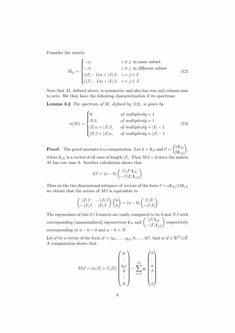
Consider the matrix

Mij =

−α; i 6= j in same subset

−β; i 6= j in different subset

(|I| − 1)α+ |J |β; i = j ∈ I(|J | − 1)α+ |I|β; i = j ∈ J.

(12)

Note that M , defined above, is symmetric and also has row and column sumto zero. We then have the following characterization if its spectrum:

Lemma 3.2 The spectrum of M , defined by (12), is given by

σ(M) =

0, of multiplicity = 1

Nβ, of multiplicity = 1

|I|α+ |J |β, of multiplicity = |I| − 1

|I|β + |J |α, of multiplicity = |J | − 1

(13)

Proof. The proof amounts to a computation. Let ~u = 1N and ~v =

(a1|I|b1|J |

),

where 1|J | is a vector of all ones of length |J |. Then M~u = 0 since the matrixM has row sum 0. Another calculation shows that

L~v = (a− b)(β |J |1|I|−β |I|1|J |

)Thus on the two dimensional subspace of vectors of the form ~v = a1|I|⊕b1|J |we obtain that the action of M~v is equivalent to(

|J |β − |J |β− |I|β |I|β

)(ab

)= (a− b)

(β |J |−β |I|

)The eigenvalues of this 2×2 matrix are easily computed to be 0 and Nβ with

corresponding (unnormalized) eigenvectors 1N and

(|J |1|I|− |I|1|J |

)respectively

corresponding to a− b = 0 and a− b = N .

Let ~w be a vector of the form ~w = (q1, . . . , q|I|, 0, . . . , 0)t, that is ~w ∈ R|I|⊕~0.A computation shows that

M ~w = (α |I|+ β |J |)

q1...q|I|0...0

−|I|∑i=1

qi

α...αβ...β

8

Choosing ~q ∈ R|I| such that|I|∑i=1

qi = 0 we see that (α |I| + β |J |) is an

eigenvalue with a |I|−1 dimensional eigenspace since the equation|I|∑i=1

qi = 0

defines a hyperplane through the origin in R|I|.

Similarly, by considering the vector ~p = (0, . . . , 0, p1, . . . , p|J |)t ∈ ~0⊕R|J |, we

get that (α |J |+β |I|) is an eigenvalue with a |J |−1 dimensional eigenspace.

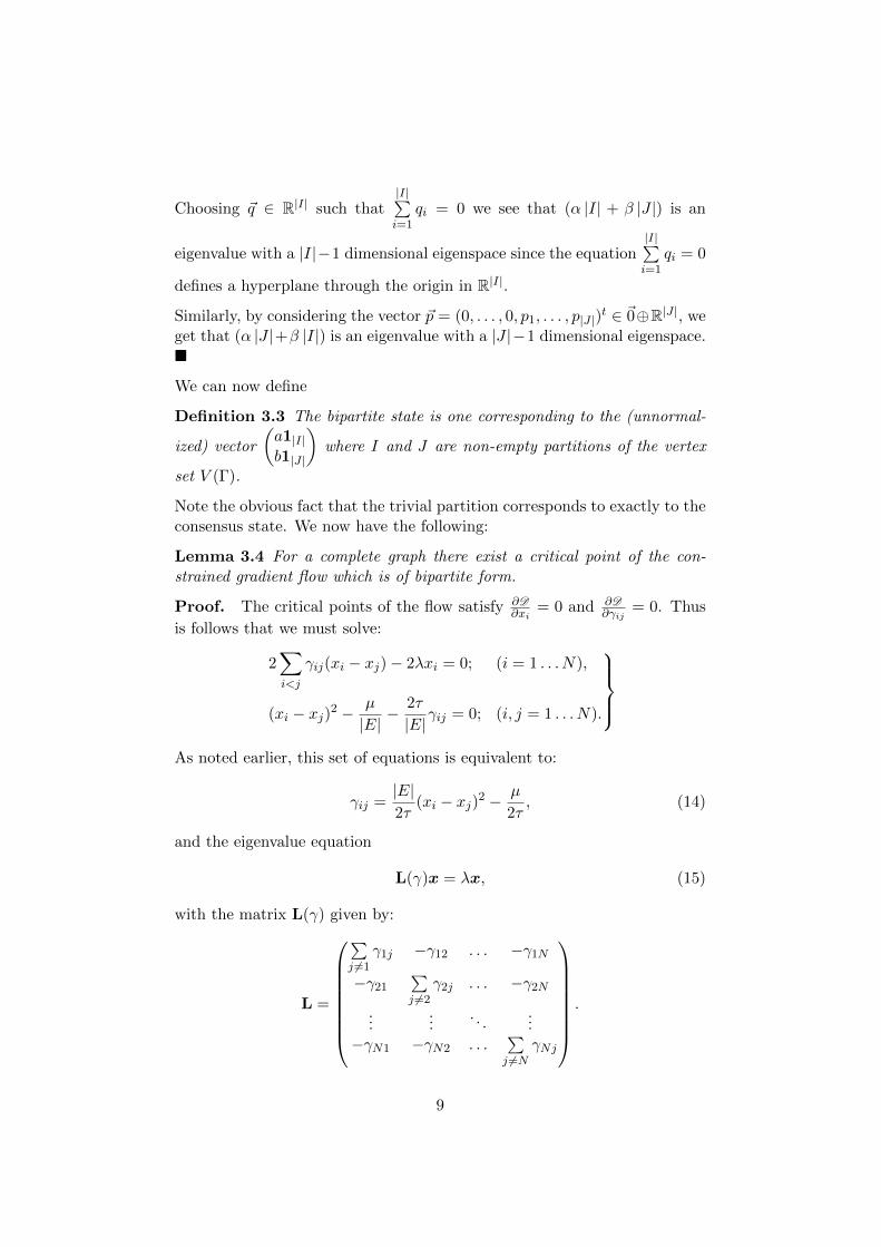
We can now define

Definition 3.3 The bipartite state is one corresponding to the (unnormal-

ized) vector

(a1|I|b1|J |

)where I and J are non-empty partitions of the vertex

set V (Γ).

Note the obvious fact that the trivial partition corresponds to exactly to theconsensus state. We now have the following:

Lemma 3.4 For a complete graph there exist a critical point of the con-strained gradient flow which is of bipartite form.

Proof. The critical points of the flow satisfy ∂D∂xi

= 0 and ∂D∂γij

= 0. Thus

is follows that we must solve:

2∑i<j

γij(xi − xj)− 2λxi = 0; (i = 1 . . . N),

(xi − xj)2 − µ

|E|− 2τ

|E|γij = 0; (i, j = 1 . . . N).

As noted earlier, this set of equations is equivalent to:

γij =|E|2τ

(xi − xj)2 − µ

2τ, (14)

and the eigenvalue equation

L(γ)x = λx, (15)

with the matrix L(γ) given by:

L =

∑j 6=1

γ1j −γ12 . . . −γ1N

−γ21∑j 6=2

γ2j . . . −γ2N

......

. . ....

−γN1 −γN2 . . .∑j 6=N

γNj

.

9

We will now show that we have a solution of the form (12). We choose theeigenvector x corresponding to the eigenvalue λ = Nβ normalized by thecontraint ‖x‖2 = R. In other words we choose

x =

√R

|J | |I|N

(|J |1|I|− |I|1|J |

).

For i 6= j in the same subsets we have that xi−xj = 0 and thus, using (14),we see that

α = − µ

2τ.

For i, j in different subsets, we see that (xi − xj)2 =RN

|I| |J |and using (14)

we get that

β =|E|2τ

RN

|I| |J |− µ

2τ.

Since the graph is complete, it follows that there are |I| (|I| − 1)/2 and|J | (|J | − 1)/2 edges in the “cliques” with |I| and |J | vertices respectively,and |I| |J | edges between the two cliques. Thus the constraints (1) and (2)then imply

Q =2

N(N − 1)

[|I| (|I| − 1)

2+|J | (|J | − 1)

2

]α+

2 |I| |J |βN(N − 1)

P =2

N(N − 1)

[|I| (|I| − 1)

2+|J | (|J | − 1)

2

]α2 +

2 |I| |J |β2

N(N − 1)

Solving this system of equations is straightforward but lengthy. When thedust settles, we obtain

α = Q± ν√

r

1− r(16)

β = Q∓ ν√

1− rr

(17)

whereν2 = P −Q2,

and

r =|I| |J ||E|

is the fraction of the total number of edges that connect the different cliques.Now

R |E|N2τ |I| |J |

= β − α = ∓ν

[√1− rr

+

√r

1− r

]

10

Hence

τ = ∓ RN

2νrk(r), (18)

and

µ = ± RN

νrk(r)

(Q± ν

√r

1− r

), (19)

while

λ := Nβ = N

(Q∓ ν

√r

1− r

)(20)

where we have defined

k(r) =

√1− rr

+

√r

1− r=

1√r(1− r)

.

This completes the proof.

4 Stability of the Consensus State

4.1 Global Stability

To motivate the results, we assume first that ε = 0 so that the gradient flowbecomes

x = −2(Lx− λx)

γij = 0.

(21)

Recall that the constraints imply x · x = 0 from which we derived

λ =〈Ly,y〉‖x‖2

.

Writing x(t) = u(t)1N + y(t) with y · 1N = 0 we see that

u = 2u〈Ly,y〉‖y‖2 +Nu2

y = −2

(Ly − y 〈Ly,y〉

‖y‖2 +Nu2

).

Let v(t) = ‖y(t)‖. It follows from the constraint that

Nu2(t) + v2(t) = Nu2(0) + v2(0) = R.

In particular

vv =1

2

d

dtv2 = −2

(〈Ly,y〉 − 〈y,y〉 〈Ly,y〉

R

),

11

which implies that

v = −2v

(1− v2

R

)〈Ly,y〉‖y‖2

.

Suppose first that v(0) = 0. Then one sees that u(t) =√

RN , that is v(t) = 0

for all t. Now assume that v(0) ∈ (0,√R] and that the matrix L has kernel

precisely 1N with all other eigenvalues positive. It then follows that

〈Ly,y〉‖y‖2

≥ σmin > 0,

from which we see that v is monotone decreasing and in particular that

v ≤ −2σminv

(1− v2(0)

R

).

A direct argument or the use of Gronwall’s inequality shows that v = 0 isexponentially attracting. Thus we have proved

Theorem 4.1 (Stability of Consensus State I) Suppose ε = 0. Sup-pose also that L(0) is positive semi-definite with a 1 dimensional kernel.Then it holds that

limt→∞

x(t) =

√R

N1N

That is, the consensus state is globally asymptotically stable.

The demonstration above relied mostly on the fact that we had a spectralgap. We know that 0 is always an eigenvalue of L but the assumption ε = 0was enough to guarantee that the next eigenvalue was strictly positive ifL(0) had all nonnegative eigenvalues. If ε 6= 0, we can still find sufficientconditions guaranteeing the existence of a spectral gap.

Theorem 4.2 (Sufficient Conditions for Global Stability) Suppose that

P −Q2

Q2<

1

N − 1.

Then L is always positive semi-definite and the consesnsus state is a globalminimizer.

Proof. For the proof we will verify that, under the stated assumption, onP,Q, L is positive semi-definite with a 1-dimensional kernel. We write eachopinion as a mean plus a mean-zero part,

γij = Q+ γij

12

where mean-zero part γij now satisfies

1

E

∑i<j

γij = 0 (22)

1

E

∑i<j

γ2ij = P −Q2. (23)

The corresponding graph Laplacian takes the form

L = L0 + L (24)

= Q

(N − 1) −1 −1 . . .−1 (N − 1) −1 . . .−1 −1 (N − 1) . . ....

......

. . .

(25)

+

∑i 6=1

γi1 −γ12 −γ13 . . .

−γ12∑i 6=2

γ12 −γ23 . . .

−γ13 −γ23∑i 6=3

γi3 . . .

......

.... . .

The important observation is that the matrix L0 commutes with every graphLaplacian, and thus they can be simultaneously diagonalized, and we needonly estimate the most negative eigenvalue of L. The latter is easily esti-mated in terms of the Hilbert-Schmidt inequality. We have

σmin(L) ≥ −

(∑i

(σi(L)

)2) 1

2

= −‖L‖HS

and

‖L‖2HS =∑i,j

γ2ij +

∑i

∑j 6=i

γij

2

≤∑i,j

γ2ij +

∑i

∑j 6=i

γ2ij

(N − 1)

≤ 2E(P −Q2) + 2(N − 1)E(P −Q2)

≤ 2NE(P −Q2)

This gives the inequality for L that the minimum eigenvalue, other than thezero eigenvalue of course, satisfies the estimate

σmin(L) ≥ N(Q−

√(N − 1)(P −Q2)

)> 0.

13

Thus once again we have a spectral gap and the proof of Theorem 4.1 canbe repeated almost verbatim.

There is a nice geometric interpretation of this result. As we have alreadyobserved, the constraint g1 = Q defines a hyperplane in R|E| while theconstraint g2 = P defines a sphere of radius

√P in R|E|. If P = Q2,

then they intersect tangentially at the single point γ∗ij = Q, i.e. γ∗ =Q(1, 1, . . . , 1)t. Note that L(γ∗ij) = L0 and that the spectrum of L0 consistsof 0 which is simple and NQ of multiplicity N − 1. This is clearly positivesemi-definite with a one dimensional kernel as long as Q > 0. What we havereally shown is that for P − Q2 ∼ small then L still satisfies this propertyas well.

Theorem 4.3 Let ε > 0 be arbitrary but fixed. Suppose that σmin(M(0)) >0 i.e., L(0) is positive semi-definite with a 1 dimensional kernel. Then thereis a positive δ = δ(ε, σmin(M(0)), R,N, P,Q) such that θ = 0 is attractingin the neighborhood Nδ(0). In other words, if L(0) satisfies the stated hy-pothesis then the consensus state is locally stable.

5 Stability of The Bipartite State

In this section we shall address the issue of stability of the explicitly con-structed bipartite states. The approach is to linearize the flow about thebipartite equilibria and to count the number of negative eigenvalues, i.e. theindex, of the resulting linear map.

Recall that the critical points of the flow are precisely the constrained ex-trema of the Dirichlet energy D i.e. the critical points of D . The methodof Lagrange multipliers and a standard Lyapunov function argument givesthe following result

Lemma 5.1 Let ω0 ∈ Ω be a critical point of D i.e. a local extrema of Dsubject to the constraints (1), (2), (3). Let the associated Hessian

H(ω0) = −

∂2D

∂xi∂xk

∂2D

∂γlk∂xi

ε∂2D

∂xk∂γijε

∂2D

∂γlk∂γij

∣∣∣∣∣∣∣∣∣∣ω0

. (26)

Let Tω0Ω be the tangent space to Ω at ω0. If H(ω0)|Tω0Ω is negative definite,

then the gradient flow is stable near ω0.

Thus we need only determine the number of negative eigenvalues of theHessian, H, restricted to TΩ. To facilitate the computation we need thefollowing

14

Lemma 5.2 Let A be a symmetric invertible matrix in Rn. Given anylinear subspace S ⊂ Rn then

n±(A) = n±(A|S) + n±(A−1∣∣S⊥

).

5.1 Index of the Full Hessian

We first put coordinates on R|E| by ordering the pairs (i, j) with i < jlexicographically. That is we write

γ = (γ12, γ13, . . . , γ23, γ24, . . . , γ34, . . .).

A direct computation shows that

∂2xD = 2(L(γ)− λ) and ∂2

γD = − 2τ

|E|I|E|×|E|.

Furthermore

∂2D

∂γlk∂xi= 2(xi − xj)δij,lk, and

∂2D

∂xk∂γij= 2(xi − xj)(δik − δjk).

Recall that the bipartite equilibrium is given by

x =

√R

|J | |I|N

(|J |1|I|− |I|1|J |

).

Defining the N × |E| matrix B with entries

Bi,lk = 2

√RN

|J | |I|

1 i ∈ l, k; i ∈ I; l, k \ i ∈ J−1 i ∈ l, k; i ∈ J ; l, k \ i ∈ I,

(27)

we see that ∂2D∂γlk∂xi

= Bi,lk. To summarize, we have shown that

H =

−2(L(γ)− λ) −B−εBt 2ετ

|E|I|E|×|E|

.

The next result will prove useful in simplifying the computations:

Lemma 5.3 (Schur Formula) Suppose that M is a symmetric matrix ofthe form

M =

(A BBt C

)where A, B and C are m×m, m× k and k× k matrices respectively and Cis invertible. Then

n±(M) = n±(C) + n±(A−BC−1Bt).

15

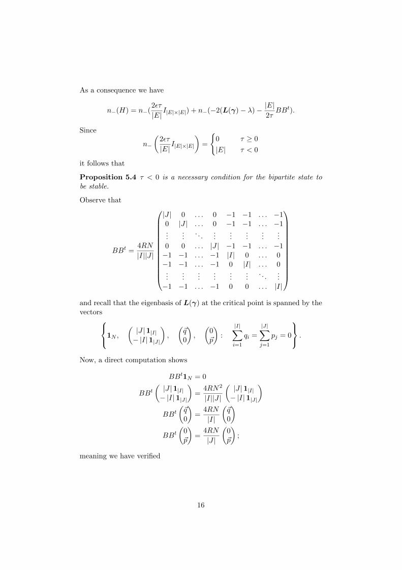
As a consequence we have

n−(H) = n−(2ετ

|E|I|E|×|E|) + n−(−2(L(γ)− λ)− |E|

2τBBt).

Since

n−

(2ετ

|E|I|E|×|E|

)=

0 τ ≥ 0

|E| τ < 0

it follows that

Proposition 5.4 τ < 0 is a necessary condition for the bipartite state tobe stable.

Observe that

BBt =4RN

|I||J |

|J | 0 . . . 0 −1 −1 . . . −10 |J | . . . 0 −1 −1 . . . −1...

.... . .

......

......

...0 0 . . . |J | −1 −1 . . . −1−1 −1 . . . −1 |I| 0 . . . 0−1 −1 . . . −1 0 |I| . . . 0...

......

......

.... . .

...−1 −1 . . . −1 0 0 . . . |I|

and recall that the eigenbasis of L(γ) at the critical point is spanned by thevectors1N ,

(|J |1|I|− |I|1|J |

),

(~q0

),

(0~p

):

|I|∑i=1

qi =

|J |∑j=1

pj = 0

.

Now, a direct computation shows

BBt1N = 0

BBt

(|J |1|I|− |I|1|J |

)=

4RN2

|I||J |

(|J |1|I|− |I|1|J |

)BBt

(~q0

)=

4RN

|I|

(~q0

)BBt

(0~p

)=

4RN

|J |

(0~p

);

meaning we have verified

16

Proposition 5.5 The matrix BBt and L(γ) have the same eigen-basis. Inparticular the spectrum of BBt is given by

σ(BBt) =

0, of multiplicity = 1

4RN2

|I||J |, of multiplicity = 1

4RN

|I|, of multiplicity = |I| − 1

4RN

|J |, of multiplicity = |J | − 1.

(28)

Since λ = Nβ for the bipartite state, it follows that the spectrum of (L(γ0)−λ) + |E|

4τ BBt is contained in the set−Nβ, N2R

rτ,

RN

2rτ(2 |J | − |I|), RN

2rτ(2 |I| − |J |)

,

the latter two being repeated |I| − 1 and |J | − 1 times respectively. For|I| > 2N/3, we see that 2 |J | − |I| < 0 and for |I| < N/3, we see that2 |I| − |J | < 0. Putting all this information together we have proven

Proposition 5.6 Assume τ < 0. For convenience put

T = −2(L(γ)− λ)− |E|2τ

BBt.

Then

n−(T ) =

|J | − 1, |I| ∈ [1, N/3)

0, |I| ∈ (N/3, 2N/3)

|I| − 1, |I| ∈ (2N/3, N − 1]

for β > 0; (29)

and

n−(T ) =

|J | , |I| ∈ [1, N/3)

1, |I| ∈ (N/3, 2N/3)

|I| , |I| ∈ (2N/3, N − 1]

for β < 0. (30)

As a consequence we have the following

Corollary 5.7 Assume τ < 0. If |I| = 1 or |I| = N − 1 then n−(H) =|E|+N − 2 for β > 0 and n−(H) = |E|+N − 1 for β < 0.

5.2 Index of the “Reduced Hessian”

Our goal now is to compute the index: n−(H|(Tω0 (Ω))⊥) of the Hessian

restricted to the orthogonal complement of Tω0(Ω). We begin with

17

Lemma 5.8 Let ω0 be the bipartite critical point and put S = Tω0(Ω). IfH is invertible then

n−(H−1∣∣S⊥

)+(∇(µ,τ,λ)(g1, g2, g3)t).

Proof. This is really a fact from the method of Lagrange multipliers amdthe thery of constrained optimization in general. First note that

∇(x,γ)D − µ∇(x,γ)g1 − τ∇(x,γ)g2 − λ∇(x,γ)g3 = 0,

and in general we can determine (x,γ) = (x(τ, µ, λ),γ(τ, µ, λ)) as func-tions of the Lagrange multipliers. Differentiating the above expression withrespect to, say, µ by the usual chain rule gives

−H · ∂x∂µ

= ∇(x,γ)g1,

and since H is invertible we see that

−∂x∂µ

= H−1 · ∇(x,γ)g1.

Similarly

−∂x∂τ

= H−1 · ∇(x,γ)g2, and − ∂x

∂λ= H−1 · ∇(x,γ)g3.

Since S⊥ is spanned by ∇(x,γ)gi3i=1, any ~v ∈ S⊥ can be written as ~v =∑i αidgi. Consequently

H−1∣∣S⊥×S⊥ = (H−1~v,~v)

=

⟨H−1

(3∑i=1

αi∇(x,γ)gi

),

3∑j=1

αj∇(x,γ)gj

⟩

= −∑i,j

αiαj

⟨∂x

∂µi,∇(x,γ)gj

⟩= −

∑i,j

αiαj∂gj∂µi

= − ∇(µ,τ,λ)(g1, g2, g3)t∣∣R3×R3 ,

whence the result.

Next recall that we have the following set of equations

µ+ 2τM1 = NR

µM1 + 2τM2 = Rλ

λ

N+

µ

2τ=RN

2rτ

18

Solving for R, P and Q and using the fact that g1 = Q, g2 = P and g3 = R,we get

g1(µ, τ, λ) =rλ

N− µ(1− r)

2τ(31)

g2(µ, τ, λ) =rλ2

N2+µ2(1− r)

4τ2(32)

g3(µ, τ, λ) =2rτ

N

(λ

N+

µ

2τ

). (33)

The Jacobian is

∂g3

∂λ

∂g3

∂µ

∂g3

∂τ

∂g1

∂λ

∂g1

∂µ

∂g1

∂τ

∂g2

∂λ

∂g2

∂µ

∂g2

∂τ

=

2rτ

N2

r

N

2rλ

N2

r

N−(1− r)

2τ

µ(1− r)2τ2

2rλ

N2

µ(1− r)2τ2

µ2(1− r)2τ3

(34)

and computing the determinant of the principal minors we get

∆1 =2rτ

N2; ∆2 = − r

N; and ∆3 =

2r2(1− r)N2τ

(µ

2τ+λ

N

)2

.

Thus for τ < 0, we see that n−(H−1∣∣S⊥

) = 2 and if in addition β < 0, weget

n−(H(ω0)|Tω0Ω) = n−(H(ω0))− n−(H(ω0)|(Tω0 (Ω))⊥) = N + |E| − 3

which equals dim(Tω0Ω). As such, we have established

Theorem 5.9 Suppose that τ , β are both negative corresponding to the bi-partite state where |I| = 1 or |I| = N − 1.∗ Then this critical point is a localminimum of the constrained Dirichlet energy and as such is locally stable.If τ < 0 and β > 0 then this state has a 1-dimensional unstable manifold.

6 Numerical Simulations

All simulations are conducted on the complete graph K5, so all actors areknown to one another (N = 5, E = 10). The relevant ODEs were inte-grated with a fourth order Runge-Kutta algorithm with dt = 10−3. In each

∗It might be more apt to call this particular state an “ostracized state” but perhapsthis has a strong negative connotation.

19

case the initial positions xi(0) and the initial opinions γij(0) were chosenrandomly. The edges are chosen as follows: we generate a vector γ withindependent, identically distributed entries drawn from the uniform distri-bution on (−1, 1). We then removed the mean of γ, and scaled γ to have unit

length. The edge weights were taken to be (P −Q2)12γ + Q(1, 1, 1, . . . , 1)t,

so that the resulting edge weights have mean Q and variance P −Q2. Thepositions were chosen uniformly from (−1, 1) with no mean.

The first set of graphs show the evolution of the positions (vertex weights)and opinions (edge weights) for an initial condition that converges to a con-sensus state. Note that initially two opinions γij are negative, and systemconverges to a stable consensus state with one negative opinion. This illus-trates that the model can accomodate a certain amount of imbalance if aconsensus is reached: actors can overcome a some antipathy if they have acommon cause.

10 20 30 40 50 60

-1.0

-0.5

0.5

VertexValues

10 20 30 40 50 60

0.5

1.0

1.5

2.0

Edge Weights

Figure 1: The evolution of the positions (top) and opinions (bottom) forinitial conditions that converge to a consensus.

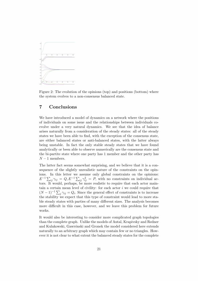
The second numerical experiment shows the dynamics in a case where theinitial variance in the opinions, P −Q2, is larger. In this case the dynamicsdoes not converge to a consensus but rather to a balanced non-consensusstate. In this case the actors divide into two parties, one with 4 individualsand one with a single individual, where each actor has a positive opinionof the actors in the same camp and a negative opinion of the actors in theother camp.

We have also considered a related system where there are contraints placedon each individual actor, not just on the actors as a group.

20

10 20 30 40 50 60

-0.5

0.5

1.0

10 20 30 40 50 60

-0.5

0.5

1.0

1.5

2.0

2.5

3.0

Figure 2: The evolution of the opinions (top) and positions (bottom) wherethe system evolves to a non-consensus balanced state.

7 Conclusions

We have introduced a model of dynamics on a network where the positionsof individuals on some issue and the relationships between individuals co-evolve under a very natural dynamics. We see that the idea of balancearises naturally from a consideration of the steady states: all of the steadystates we have been able to find, with the exception of the consensus state,are either balanced states or anti-balanced states, with the latter alwaysbeing unstable. In fact the only stable steady states that we have foundanalytically or been able to observe numerically are the consensus state andthe bi-partite state where one party has 1 member and the other party hasN − 1 members.

The latter fact seems somewhat surprising, and we believe that it is a con-sequence of the slightly unrealistic nature of the constraints on the opin-ions. In this letter we assume only global constraints on the opinions:E−1

∑ij γij = Q,E−1

∑ij γ

2ij = P, with no constraints on individual ac-

tors. It would, perhaps, be more realistic to require that each actor main-tain a certain mean level of civility: for each actor i we could require that(N − 1)−1

∑j γij = Qi. Since the general effect of constraints is to increase

the stability we expect that this type of constraint would lead to more sta-ble steady states with parties of many different sizes. The analysis becomesmore difficult in this case, however, and we leave this problem for futureworks.

It would also be interesting to consider more complicated graph topologiesthan the complete graph. Unlike the models of Antal, Krapivsky and Rednerand Kulakowski, Gawronski and Gronek the model considered here extendsnaturally to an arbitrary graph which may contain few or no triangles. How-ever it is not clear to what extent the balanced steady states for the complete

21

graph persist in these more sparse graph topologies.

References

[1] T. Antal, P.L. Krapivsky, and S. Redner. Dynamics of social balanceon networks. Phys. Rev. E., 72, 2005.

[2] R. Axelrod. The dissemination of culture: A model with local conver-gence and global polarization. J. Conflict Resolution, 41(2), 1997.

[3] D. Cartwright and F. Harary. Structural balance: A generalization ofheider’s theory. Psychological Review, 63:277–293, 1956.

[4] C. Castellano, S. Fortunato, and V. Loreto. Statistical physics of socialdynamics. Reviews of Modern Physics, 81:591–645, 2009.

[5] C. Castellano, M. Marsili, and A. Vespignani. Nonequilibrium phasetransition in a model for social influence. Phys. Rev. Lett., 85(16), 2000.

[6] S.N. Durlauf. How can statistical mechanics contribute to social sci-ence? Proc. Nat. Acad. Sci. USA, 96:10582–10584, 1999.

[7] S. Galam. Social paradoxes of majority rule voting and renormalizationgroup. J. Stat. Phys., 61:943–951, 1990.

[8] S. Galam. A review of galam models. Int. J. Mod. Phys. C, 19:409–440,2008.

[9] F. Heider. Attitudes and cognitive organization. Journal of Psychology,pages 107–112, 1946.

[10] K. Kulakowski, P. Gawronski, and P. Gronek. The hedier balance:A continuous approach. International Journal of Modern Physics C.,16(05), 2005.

[11] S. Marvel, J. Kleinberg, R.D. Kleinberg, and S. Strogatz. Continuous-time model of structural balance. Proceedings of the National Academyof Sciences, 108:1771–1776, 2010.

[12] S. Marvel, S. Strogatz, and J. Kleinberg. Energy landscape of socialbalance. Physical Review Letters, 103, 2009.

[13] M Mobilia. Does a single zealot affect an infinite group of voters. Phys.Rev. Lett., 91, 2003.

[14] F. Shi, P.J. Mucha, and R. Durrett. Multiopinion coevolving votermodel with infinitely many phase transitions. Phys. Rev. E, 88, 2013.

22

[15] W. Zhang, C. Lim, S. Screenivasan, J. Xie, B.K. Szymanski, and G. Ko-rniss. Social influencing and associated random walk models: Asymp-totic consensus times on the complete graph. Chaos, 21, 2011.

8 Appendix

In this section we show the existence of a locally attracting neighborhoodof the consensus state. The argument is similar in spirit to that for globalstability. The main complication is that we have to explicitly handle theevolution equation for the spectrum of L.

For convenience, we define 1N = 1√N

1N to be the normalized vector of all

ones. Let W = y ∈ RN |y · 1N = 0 be the subspace of vectors orthogonalto the “consensus state”. Following a similar argument as before, we willwrite

x = c(cos(θ)1N + sin(θ)y

)with y ∈W and ‖y‖ = 1. The goal is to show that θ → 0 which will implythe stability of the consensus state. We will first obtain equations governingthe dynamics of the relevant variables.

From the constraint x · x = 0, it follows that

λ = sin2(θ) 〈Ly,y〉 .

The original equation x = −2(L~x − λx) and the fact that L1N = 0 thenimplies(− sin(θ)θ1N + cos(θ)θy + sin(θ)y

)= −2

(sin(θ)Ly − λ

(cos(θ)1N + sin(θ)y

)).

Taking the inner product of the above equation with 1N and simplifyinggives

θ = − sin(2θ)(Ly,y). (35)

Using the equation for θ, we can also determine that

y = −2(L~y − 〈Ly,y〉y). (36)

We define e(t) = 〈L(t)y(t),y(t)〉 and we note that e(t) takes values in thenumerical range of L(t). Put M = L|W . Since L is symmetric with realentries and since y ∈W , we have the bound

σmin(L(t)) ≤ σmin(M(t)) ≤ e(t) ≤ σmax(M(t)) ≤ σmax(L(t)). (37)

We shall occasionally make use of the following result which allows us toestimate the spectrum of a matrix in terms of its entries:

23

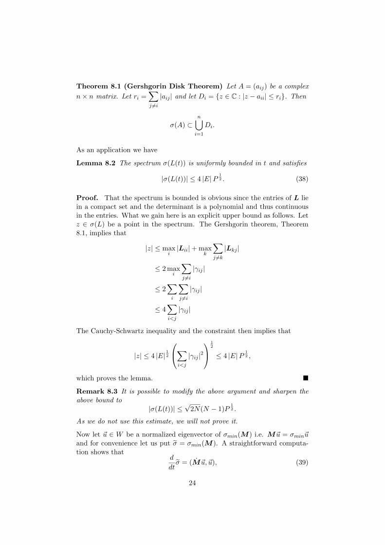
Theorem 8.1 (Gershgorin Disk Theorem) Let A = (aij) be a complex

n× n matrix. Let ri =∑j 6=i|aij | and let Di = z ∈ C : |z − aii| ≤ ri. Then

σ(A) ⊂n⋃i=1

Di.

As an application we have

Lemma 8.2 The spectrum σ(L(t)) is uniformly bounded in t and satisfies

|σ(L(t))| ≤ 4 |E|P12 . (38)

Proof. That the spectrum is bounded is obvious since the entries of L liein a compact set and the determinant is a polynomial and thus continuousin the entries. What we gain here is an explicit upper bound as follows. Letz ∈ σ(L) be a point in the spectrum. The Gershgorin theorem, Theorem8.1, implies that

|z| ≤ maxi|Lii|+ max

k

∑j 6=k|Lkj |

≤ 2 maxi

∑j 6=i|γij |

≤ 2∑i

∑j 6=i|γij |

≤ 4∑i<j

|γij |

The Cauchy-Schwartz inequality and the constraint then implies that

|z| ≤ 4 |E|12

∑i<j

|γij |2 1

2

≤ 4 |E|P12 ,

which proves the lemma.

Remark 8.3 It is possible to modify the above argument and sharpen theabove bound to

|σ(L(t))| ≤√

2N(N − 1)P12 .

As we do not use this estimate, we will not prove it.

Now let ~u ∈ W be a normalized eigenvector of σmin(M) i.e. M~u = σmin~uand for convenience let us put σ = σmin(M). A straightforward computa-tion shows that

d

dtσ = (M~u, ~u), (39)

24

where M is the matrix obtained by differentiating the entries of M withrespect to t. The Gershgorin theorem, as in the proof of Lemma 8.2, implies∣∣∣∣ ddt σ

∣∣∣∣ ≤ |(M~u, ~u)| ≤ |σ(L)| ≤ 4∑i<j

|γij | .

We note the following simple lemma which will allow us to simply the variousexpressions

Lemma 8.4 Let x =√R(cos(θ)1N + sin(θ)y

)with y ∈ W and ‖y‖ = 1.

Then ∑i<j

(yi − yj)2 = N,

and thus ∑i<j

(xi − xj)2 = R sin2(θ).

A direct substitution shows that

γij = −εR sin2(θ)

[(yi − yj)2 − (PN −Qe) + γij(e−QN)

|E| (P −Q2)

],

and thus

|γij | ≤ εR sin2(θ)

[(yi − yj)2 +

|PN −Qe|+ |γij | |e−QN ||E| (P −Q2)

],

which in turn implies, using the constraints, Lemma 8.4 and the CauchySchwartz inequality that

∑i<j

|γij | ≤ εR sin2(θ)

∑i<j

(yi − yj)2 +|PN −Qe||E| (P −Q2)

∑i<j

1 +|e−QN ||E| (P −Q2)

∑i<j

|γij |

≤ εR sin2(θ)

[N +

|PN −Qe|+ P12 |e−QN |

(P −Q2)

].

By Lemma 8.2, |e| ≤ 4 |E|P12 and thus the quantity in brackets in the last

inequality above is seen to be uniformly bounded. Thus for some positiveconstant K = K(R,N,P,Q) we have that∣∣∣∣ ddt σ

∣∣∣∣ ≤ εK sin2(θ) (40)

We are now ready to prove the local stability theorem.

25

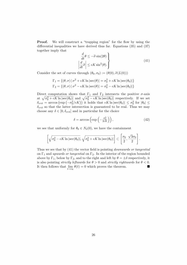
Proof. We will construct a “trapping region” for the flow by using thedifferential inequalities we have derived thus far. Equations (35) and (37)together imply that

d

dtθ ≤ −σ sin(2θ)∣∣∣∣ ddt σ∣∣∣∣ ≤ εK sin2(θ).

(41)

Consider the set of curves through (θ0, σ0) := (θ(0), σ(L(0)))

Γ1 = (θ, σ) |σ2 + εK ln |sec(θ)| = σ20 + εK ln |sec(θ0)|

Γ2 = (θ, σ) |σ2 − εK ln |sec(θ)| = σ20 − εK ln |sec(θ0)|

Direct computation shows that Γ1 and Γ2 intersects the positive σ-axisat√σ2

0 + εK ln |sec(θ0)| and√σ2

0 − εK ln |sec(θ0)| respectively. If we setδcrit = arccos

(exp

(−σ2

0/εK))

it holds that εK ln |sec(θ0)| ≤ σ20 for |θ0| ≤

δcrit so that the latter intersection is guaranteed to be real. Thus we maychoose any δ ∈ [0, δcrit] and in particular for the choice

δ = arccos(

exp(− σ2

02εK

)), (42)

we see that uniformly for θ0 ∈ Nδ(0), we have the containment[√σ2

0 − εK ln |sec(θ0)|,√σ2

0 + εK ln |sec(θ0)|]⊂

[σ0

2,

√3σ0

2

].

Thus we see that by (41) the vector field is pointing downwards or tangentialon Γ1 and upwards or tangential on Γ2. In the interior of the region boundedabove by Γ1, below by Γ2, and to the right and left by θ = ±δ respectively, itis also pointing strictly leftwards for θ > 0 and strictly rightwards for θ < 0.It then follows that lim

t→∞θ(t) = 0 which proves the theorem.

26