last revised: 30 October 2009

14 The Dynamics of Balance Theory

In some types of social networks, the links between actors can be either positive ornegative. Depending on the context, positive links might reflect friendship or alliance;negative links might reflect enmity or hostility. Balance theory attempts to explainthe structure of these networks. After briefly reviewing some core ideas of balancetheory, we develop a simple model of the adjustment process by which links mightchange sign (from positive to negative or vice versa). The model is technically anabsorbing Markov chain with 2N states (where N is the number of links). However,as we verify through simulation analysis, the behavior of this Markov chain is wellapproximated by a simple one-dimensional nonlinear model. Interestingly, given themyopic adjustment process we consider, the equilibrium of the nonlinear model maydiffer from the long-run outcome (“balance”) presumed by the theory.

14.1 Balance theory

In his seminal contribution to balance theory, Heider (1946) focused on a simple socialnetwork with three actors (i.e., a triad) in which each pair of actors is connected byeither a positive or negative link. Graphically, we may use solid lines to denotepositive links, and dotted lines to denote negative links. Ignoring the identities ofthe actors, there are four possible types of triads, shown below.

c cc

JJ

JJ

J

0

c cc

J

JJJJ

1

c cc

2

c cc

3

Note that the index for each triad simply indicates the number of negative links.Heider argued that, from a social-psychological perspective, triads of type 0 or 2 arestable (“balanced”) while triads of type 1 or 3 are not. Essentially, type-1 triadsare imbalanced because they violate the principle that “a friend of my friend is myfriend.” If the network started as a type-1 triad, balance might be achieved eitherby making the negative link positive (so that the network becomes a type-0 triad) orby making one of the positive links negative (so that the network becomes a type-2triad). Essentially, type-3 triads are imbalanced because they violate the principlethat “an enemy of my enemy is my friend.” If the network started as a type-3 triad,

1

we might thus anticipate that one of the negative links will become positive, so thatthe network is transformed into a type-2 triad. In contrast, because triads of type 0and 2 satisfy both of these principles, we have no reason to expect any change in thesign of the links. Given enough time for social-psychological forces to “play out,” wemight thus expect to observe only balanced triads (type 0 or 2) in the long run.1

In another seminal paper, Cartwright and Harary (1956) formalized Heider’sintuition, and extended the concept of balance to larger networks. Interestingly,their concept of balance can be stated in two equivalent ways. The first requiressome terminology from graph theory. A cycle is a sequence of links that begins andends at the same node. For a signed graph (i.e., a network in which links are eitherpositive or negative), the sign of a cycle is given by the product of the signs of thelinks that comprise the cycle. To illustrate, consider again the 4 types of triads.From the diagram above, it is apparent that type-0 triads contain a positive cycle(schematically, + ·+ ·+ = +), type-1 triads contain a negative cycle (+ ·+ ·− = −),type-2 triads contain a positive cycle (+ · − · − = +), and type-3 triads contain anegative cycle (− · − · − = −). This suggests that the balance of a signed graphdepends on the signs of its cycles. More precisely, following the definition developedby Cartwright and Harary, a signed graph is balanced if and only if every cycleis positive. Importantly, this definition allows us to move beyond triads, assessingbalance for social networks with any number of actors.2

Balance can also be assessed in a second way. Again following Cartwright andHarary (1956), a signed graph is balanced if and only if the nodes can be partitionedinto two subsets (one possibly empty), with any positive links connecting nodeswithin subsets, and any negative links connecting nodes between subsets. Intuitively,the network is balanced when the actors can be separated into (no more than) two“camps” in such a way that any friends belong to the same camp and any enemiesbelong to different camps. Returning to our 4 types of triads, note that this partitionis possible for triads of type 0 (where all actors belong to the same camp) and type2 (where 2 actors belong to one camp and the remaining actor belongs to the othercamp). However, this partition is not possible for triads of type 1 or 3.3 Like the“cycle” criterion discussed above, the “partition” criterion can also be used to assessbalance in networks with any number of actors.4

1Against Heider (1946), some researchers (notably Davis 1967) have argued that type-3 triadsare not inherently unstable. This leads to a variation on balance called “clusterability.” For thepresent chapter, we focus on Heider’s original conception of balance.

2For a signed graph with many nodes, some cycles may be quite long. This makes it difficultto assess balance merely by inspecting the graph. However, researchers have developed algebraicprocedures for assessing balance (see Harary et al 1965, Batagelj 1994, Montgomery 2009).

3For the type-1 triad, suppose we label the actors {A,B,C} so that there is a positive link fromA to B, a positive link from B to C, and a negative link from A to C. By virtue of the positivelinks, both A and C should be placed in B’s camp. But the negative link from A to C makes thisimpossible. For the type-3 triad, we can eliminate negative links within camps only if there are 3different camps. But balance permits at most 2 camps.

4While the equivalence of the cycle and partition criteria may not be immediately obvious, this is

2

Cartwright and Harary (1956) did not presume that the network is complete (i.e.,that every pair of actors is connected by either a positive or negative link). However,if we restrict attention to complete networks, the balance criterion may be statedin yet another way. A complete network with n actors has n(n − 1)/2 links andn(n− 1)(n− 2)/6 triads. As first noted by Flament (1963), a complete signed graphis balanced if and only if every triad is balanced. To assess balance using this “triad”criterion, we can conduct a triad census, counting the number of triads of each ofthe 4 possible types. The network is balanced if and only if every triad is of type0 or 2 (and hence no triads are of type 1 or 3). Moreover, a simple measure of the“degree” of balance is given by the proportion of triads that are balanced.

14.2 A process model

Given that background, we might view “balance” as a conjecture about the structureof the network in the long run. However, without a specification of the process bywhich links are altered, it is unclear whether this outcome will actually be reached.While researchers have proposed a variety of adjustment mechanisms, this sectionconsiders a very simple “myopic” specification from Antal et al (2006).

For simplicity, we assume a complete network, so that each pair of actors isconnected by either a positive or negative link. Each period, we randomly select onetriad. If this triad is balanced (type 0 or 2), no links are altered. If the triad is type3, then one of the negative links (chosen at random) becomes positive. If the triad istype 1, then the negative link becomes positive with probability p. Otherwise (withprobability 1 − p), one of the positive links (chosen at random) becomes negative.Our adjustment process is thus summarized by the following diagram.

c cc

JJ

JJ

J

0

c cc

J

JJJJ

1

c cc

2

c cc

3

� - �p 1−p 1

Note that, in the special case where p = 1/3, we simply “flip” the sign of a ran-dom edge whenever an unbalanced triad is selected. While this adjustment processensures balance of the focal triad, the process is “myopic” because any sign changecould induce imbalance in other triads. After modifying the focal triad (if it wasimbalanced), we begin the next period by randomly selecting a new focal triad. This

the content of the Structure Theorem proven by Cartwright and Harary (1956). Interested readersmight see the original paper or Chartrand (1977) for a proof.

3

adjustment process is repeated indefinitely (unless balance is achieved, in which caseno further adjustments occur).

Formally, this process constitutes a Markov chain. The states of the chain arethe possible configurations of the network. Thus, given n actors, there are 2n(n−1)/2

possible states of the chain. If the number of actors is very small (say n = 3 or4), we could analyze this model using the (transition matrix) method developed inChapter 4. Given larger n, this approach is clearly impractical. However, based onour knowledge of Markov chains, we can still say something qualitative about thelong-run behavior of this chain. From the description of the adjustment process, itis apparent that balanced states (in which all triads are positive) are absorbing, thatimbalanced states (in which some triads are negative) are transitory, and that everyimbalanced state can reach (directly or indirectly) a balanced state. Thus, we knowthat the chain will eventually be absorbed if the process continues indefinitely.

While that conclusion is correct, it is also potentially misleading. Simulationsreveal that, when n is large and p < 1/2, balance is unlikely to occur within any“empirically relevant” time frame.5 Rather, over the course of a (very long) sim-ulation run, the system appears to converge to a (stochastic) steady state with aconstant proportion of positive links, and a degree of balance below 1. To illustrate,we use the m-file balancedynamics placed in Appendix xx.

>> help balancedynamics

[d, y] = balancedynamics(p, x0, n, T)balance theory simulation model based on Antal et al (2006)input p = probability that type-1 triad becomes type-0 triadinput x0 = probability that each link is initially positiveinput n = number of actorsinput T = number of iterationsoutput d is a T x 4 matrix giving triad census [d0 d1 d2 d3] for each periodoutput y is a vector of length T giving number of positive links for each period

This program begins by constructing a random graph with n nodes (and hencen(n−1)/2 links) in which each link is positive with probability x0 (and hence negativewith probability x0). It then implements (for T iterations) the adjustment processdescribed above so that a type-1 triad becomes a type-0 triad with probability p(and hence becomes a type-2 triad with probability 1− p). The function outputs a(T × 4) matrix d giving the triad census for each period, and a (length T ) vector ygiving the number of positive links in each period.

Setting the parameters p = 1/3, x0 = .99, n = 100, and T = 50000, the results ofone trial are shown on the next page.6 For these parameters, the total number of links

5See Antal et al (2006) for some formal analysis of the relationship between network size andexpected time to absorption.

6On my desktop computer, this run took about 10 minutes. The long computation time is due

4

>> [d, y] = balancedynamics(1/3, .99, 100, 50000);>> plot(y) % number of positive links over simulation run

0 0.5 1 1.5 2 2.5 3 3.5 4 4.5 5

x 104

2000

2500

3000

3500

4000

4500

5000

num

ber o

f pos

itive

link

s

periods

>> plot(d) % triad census over simulation run

0 0.5 1 1.5 2 2.5 3 3.5 4 4.5 5

x 104

0

2

4

6

8

10

12

14

16x 104

period

num

ber o

f tria

ds

type 0

type 1

type 2

type 3

5

is n(n− 1)/2 = 4950, and the total number of triads is n(n− 1)(n− 2)/6 = 161700.Thus, from the top diagram, we see that the share of positive links falls from itsinitial value (approximately x0 = 0.95) to a “steady state” share of approximatelyx∗ = 1/2. From the bottom diagram, we see that the shares of type-1 and type-2triads converge to approximately 3/8, while the shares of type-0 and type-3 triadsconverge to approximately 1/8.7

Further simulation runs produce quite similar results. (Readers are encouraged touse the m-file to verify this claim for themselves. In particular, you should vary x0 todemonstrate that the same imbalanced equilibrium arises for any initial condition.)Thus, for our current parameter values (p = 1/3 and n large), simulation analysissuggests that the degree of balance (i.e., the sum of the shares of type-0 and type-2triads) does not approach 1, but instead converges to 1/2. Of course, if we allowedthis simulation to continue forever, we know that the chain will eventually reach abalanced (absorbing) state. But based on even longer simulation runs (and analyticalresults from Antal et al 2006), it is apparent that the system will “hover around” animbalanced equilibrium for any “empirically relevant” time frame.

14.3 A deterministic approximation

The smooth time paths shown in the preceding diagrams might suggest the possibilityof approximating the (very high-dimensional) Markov chain process with a (hopefullylow-dimensional) nonlinear system. In fact, Antal et al (2006) have shown thatthe behavior of the process is well approximated by a one-dimensional nonlinearsystem. To begin developing this model, let xt denote the proportion of links thatare positive in period t. Assuming that process begins with a random graph (so thatthe probability of a positive realization is independent across links), we can obtaina good approximation of the triad census by viewing each triad as a sample of 3links. Following Antal et al (2006), we may say that the elements of the triad censusare initially “uncorrelated.” Interestingly, some formal analysis in Antal et al (2006)reveals that, if the elements of the triad census are initially uncorrelated, then theyremain uncorrelated indefinitely. Consequently, for any period, the triad census iswell approximated by the equations

dt(0) = xt3

dt(1) = 3xt2(1− xt)

primarily to recomputation of the triad census at every iteration. Computation time rises linearlyin T and exponentially in n.

7The share of positive links (top diagram) can be derived from the triad census (bottom diagram)using the equation

x =3d(0) + 2d(1) + d(2)

n− 2where d(i) indicates the number of triads of type i. Intuitively, each type-i triad contains 3 − ipositive links, and each link appears in n− 2 triads.

6

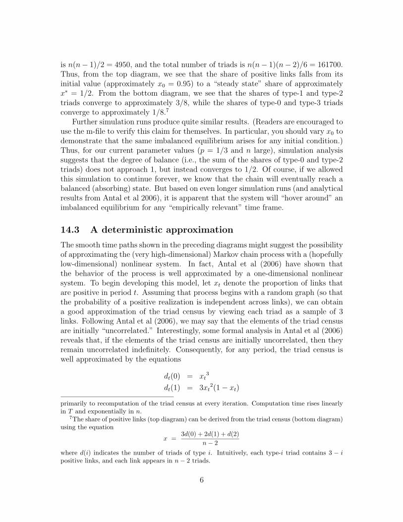
dt(2) = 3xt(1− xt)2

dt(3) = (1− xt)3

where dt(i) denotes the proportion of triads of type i in period t. Intuitively, viewinga triad as a sample of 3 links, we obtain a type-i triad when 3− i positive links andi negative links are drawn.

Because each element of the triad census depends solely on the proportion ofpositive links (x), we merely need to account for the dynamics of this one statevariable. To develop an equation, consider one iteration of the process model. If atype-1 triad is selected (this occurs with probability d(1)) then the number of positivelinks rises by 1 with probability p and falls by 1 with probability 1 − p. If a type-3triad is selected (this occurs with probability d(3)) then the number of positive linksrises by one. Thus, the expected change in the number of positive links is given by

d(1)[p− (1− p)] + d(3)

= 3x2(1− x)(2p− 1) + (1− x)3

Because x denotes the proportion (not number) of links that are positive, we needto divide this expression by the number of links in order to obtain the change in x.Doing so, we obtain our one-dimensional system

∆x =1

n(n− 1)/2

[3x2(1− x)(2p− 1) + (1− x)3

]with parameters p and n.

As a first “test” of this approximation, we compute the predicted time paths forour preceding example, which are shown on the next page. Further examples confirmthat there is a good match between simulation results and this one-dimensionalmodel. (Readers are encouraged to compare simulation results to the deterministicpredictions for different values of the parameter p and the initial condition x0. Youmight also experiment with different values of n, though computation time increasesexponentially in that parameter.)

Returning to the equation above, it is apparent that ∆x is always positive whenp > 1/2 and x 6= 1. That is, when type-1 triads are more likely to be transformedinto type-0 triads than type-2 triads, the proportion of positive links will continueto rise until all links are positive. Thus, given p > 1/2, we find that the networkdoes become balanced (within an “empirically relevant” time frame). In contrast,for p < 1/2, we see that ∆x = 0 implies x = 1 or

3x2(2p− 1) + (1− x)2 = 0

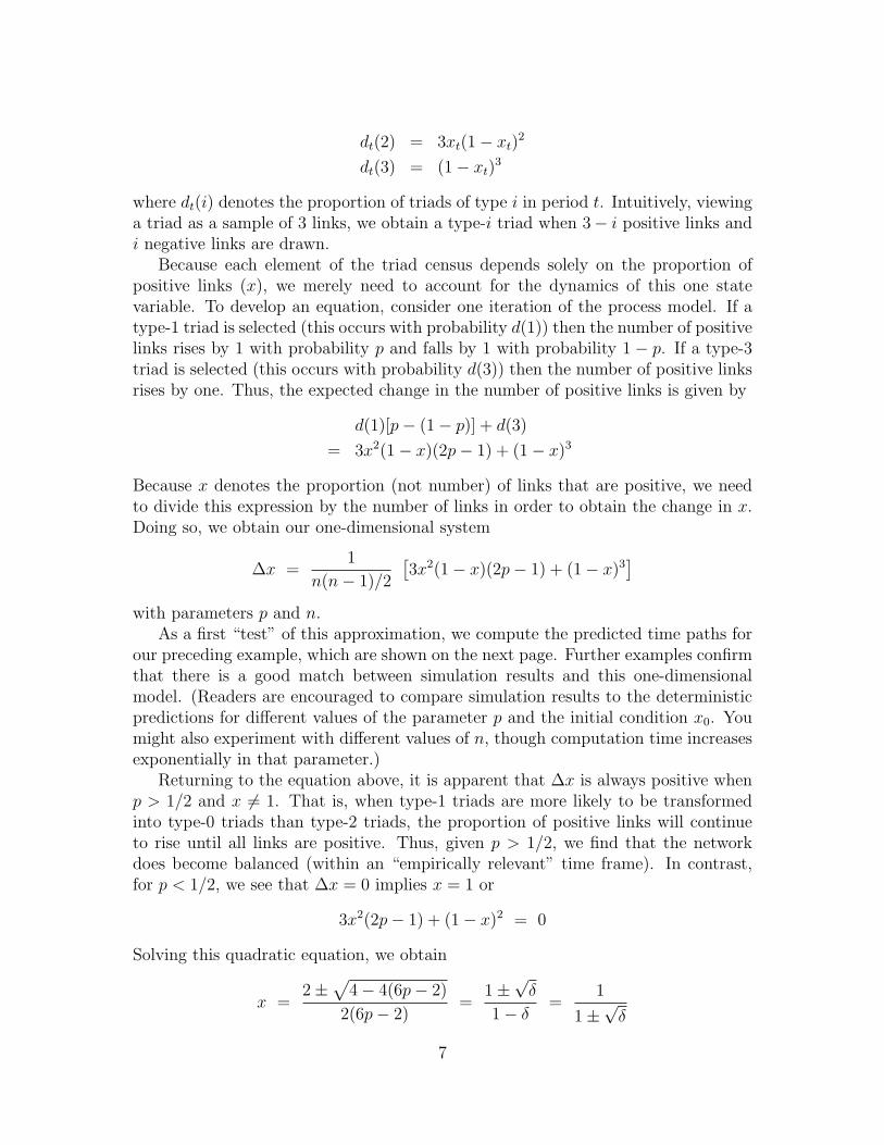
Solving this quadratic equation, we obtain

x =2±

√4− 4(6p− 2)

2(6p− 2)=

1±√

δ

1− δ=

1

1±√

δ

7

>> x = .99; p = 1/3; n = 100; L = n*(n-1)/2; y = x;for t = 1:50000; dx = (3*x^2*(1-x)*(2*p-1) + (1-x)^3)/L; x = x+dx; y = [y; x]; end>> plot(y) % time path for proportion of positive links

0 0.5 1 1.5 2 2.5 3 3.5 4 4.5 5

x 104

0.4

0.5

0.6

0.7

0.8

0.9

1

period

prop

ortio

n of

pos

itive

link

s

>> plot([y.^3, 3 * y.^2 .* (1-y), 3 * y .* (1-y).^2, (1-y).^3])>> % time paths of triad census

0 0.5 1 1.5 2 2.5 3 3.5 4 4.5 5

x 104

0

0.1

0.2

0.3

0.4

0.5

0.6

0.7

0.8

0.9

1

period

prop

ortio

n of

tria

ds

type 0

type 1

type 2

type 3

8

where δ = 3 − 6p. Focusing on the root that lies between 0 and 1, we thus obtainthe steady state

x∗ =1

1 +√

3− 6p

Because ∆x is positive for x between 0 and x∗, and is negative for x between x∗ and1, the steady state x∗ is the unique stable equilibrium.

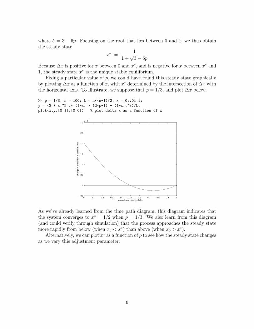
Fixing a particular value of p, we could have found this steady state graphicallyby plotting ∆x as a function of x, with x∗ determined by the intersection of ∆x withthe horizontal axis. To illustrate, we suppose that p = 1/3, and plot ∆x below.

>> p = 1/3; n = 100; L = n*(n-1)/2; x = 0:.01:1;y = (3 * x.^2 .* (1-x) * (2*p-1) + (1-x).^3)/L;plot(x,y,[0 1],[0 0]) % plot delta x as a function of x

0 0.1 0.2 0.3 0.4 0.5 0.6 0.7 0.8 0.9 1−0.5

0

0.5

1

1.5

2

2.5

3x 10−4

proportion of positive links

chan

ge in

pro

porti

on o

f pos

itive

link

s

As we’ve already learned from the time path diagram, this diagram indicates thatthe system converges to x∗ = 1/2 when p = 1/3. We also learn from this diagram(and could verify through simulation) that the process approaches the steady statemore rapidly from below (when x0 < x∗) than above (when x0 > x∗).

Alternatively, we can plot x∗ as a function of p to see how the steady state changesas we vary this adjustment parameter.

9

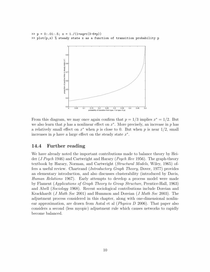
>> p = 0:.01:.5; x = 1./(1+sqrt(3-6*p))>> plot(p,x) % steady state x as a function of transition probability p

0 0.05 0.1 0.15 0.2 0.25 0.3 0.35 0.4 0.45 0.50.3

0.4

0.5

0.6

0.7

0.8

0.9

1

probability of transition from type−1 to type−0 (p)

prop

ortio

n of

pos

itive

link

s in

ste

ady

stat

e (x

*)

From this diagram, we may once again confirm that p = 1/3 implies x∗ = 1/2. Butwe also learn that p has a nonlinear effect on x∗. More precisely, an increase in p hasa relatively small effect on x∗ when p is close to 0. But when p is near 1/2, smallincreases in p have a large effect on the steady state x∗.

14.4 Further reading

We have already noted the important contributions made to balance theory by Hei-der (J Psych 1946) and Cartwright and Harary (Psych Rev 1956). The graph-theorytextbook by Harary, Norman, and Cartwright (Structural Models, Wiley, 1965) of-fers a useful review. Chartrand (Introductory Graph Theory, Dover, 1977) providesan elementary introduction, and also discusses clusterability (introduced by Davis,Human Relations 1967). Early attempts to develop a process model were madeby Flament (Applications of Graph Theory to Group Structure, Prentice-Hall, 1963)and Abell (Sociology 1968). Recent sociological contributions include Doreian andKrackhardt (J Math Soc 2001) and Hummon and Doreian (J Math Soc 2003). Theadjustment process considered in this chapter, along with one-dimensional nonlin-ear approximation, are drawn from Antal et al (Physica D 2006). That paper alsoconsiders a second (less myopic) adjustment rule which causes networks to rapidlybecome balanced.

10

14.5 Appendix

14.5.1 Balancedynamics m-file

function [d, y] = balancedynamics(p, x0, n, T)% [d, y] = balancedynamics(p, x0, n, T)% balance theory simulation model based on Antal et al (2006)% input p = probability that type-1 triad becomes type-0 triad% input x0 = probability that each link is initially positive% input n = number of actors% input T = number of iterations% output d is a T x 4 matrix giving triad census [d0 d1 d2 d3] for each period% output y is a vector of length T giving number of positive links for each period

L = n*(n-1)/2; % number of linksA = rand(n) < x0; A = triu(A,1); % initial random graph

y = []; d = [];for t = 1:T

y = [y; sum(sum(A))]; % count number of positive links

P = A|A’; N = ~P - eye(n);d0 = trace(P*P*P)/6; d1 = trace(P*P*N)/2; d2 = trace(P*N*N)/2; d3 = trace(N*N*N)/6;d = [d; d0 d1 d2 d3]; % triad census

v = randperm(n); v = v(1:3); v = sort(v);s12 = A(v(1),v(2)); s23 = A(v(2),v(3)); s13 = A(v(1),v(3)); s = s12 + s23 + s13;

if s == 1 | s == 3 % triad is balancedcontinue

end

r = rand;

if s == 0 % all edges are negativeif r < 1/3

A(v(1),v(2)) = 1;elseif r < 2/3

A(v(2),v(3)) = 1;else

A(v(1),v(3)) = 1;end

end

if s == 2 % one edge is negativeif s12 == 0

if r < .5*(1-p)A(v(2),v(3)) = 0;

elseif r < (1-p)A(v(1),v(3)) = 0;

11

elseA(v(1),v(2)) = 1;

endelseif s23 == 0

if r < .5*(1-p)A(v(1),v(2)) = 0;

elseif r < (1-p)A(v(1),v(3)) = 0;

elseA(v(2),v(3)) = 1;

endelse

if r < .5*(1-p)A(v(1),v(2)) = 0;

elseif r < (1-p)A(v(2),v(3)) = 0;

elseA(v(1),v(3)) = 1;

endend

endend

12