embodied energy calculation: method and guidelines …
TRANSCRIPT
EMBODIED ENERGY CALCULATION: METHOD AND GUIDELINES FOR A
BUILDING AND ITS CONSTITUENT MATERIALS
A Dissertation
by
MANISH KUMAR DIXIT
Submitted to the Office of Graduate and Professional Studies of
Texas A&M University
in partial fulfillment of the requirements for the degree of
DOCTOR OF PHILOSOPHY
Approved by:
Chair of Committee, Charles H. Culp
Co-Chair of Committee, José L. Fernández-Solís
Committee Members, David E. Claridge
Mark J. Clayton
Wei Yan
Head of Department, Ward Wells
December 2013
Major Subject: Architecture
Copyright 2013 Manish Kumar Dixit

ii
ABSTRACT
The sum of all energy embedded in products and processes used in constructing a building is known as
embodied energy. According to the literature, the current state of embodied energy research suffers from
three major issues. First, there is little agreement on the definition of embodied energy. Second, the
existing embodied energy data suffers from variation and are regarded as incomplete and not specific to a
product under study. Third, there are various methods for calculating embodied energy with varying levels
of completeness and accuracy. According to the literature, the input-output-based hybrid method is the
most appropriate method but it needs further improvements. Some of the studies also found a positive and
strong correlation between the cost and embodied energy of a building but this correlation needs to be
analyzed at a building material or product level.
This research addressed the three issues identified by the literature. First, using a rigorous literature
survey, it proposed an embodied energy definition, a complete system boundary model, and a set of data
collection, embodied energy calculation, and result reporting guidelines. The main goal of proposing the
guidelines was to streamline the process of embodied energy calculation to reduce variations in embodied
energy data. Second, three improvements were carried out in the current input-output-based hybrid
approach, which included process energy data inclusion, human and capital energy integration, and
sectorial disaggregation to calculate material-specific embodied energy. Finally, the correlation between
the embodied energy and cost and price was analyzed at a material level.
The study concluded that an input-output-based hybrid method was the most appropriate method for
calculating the embodied energy of a building material in a complete manner. Furthermore,
incompleteness in the results of a process-based method was significant (3.3 to 52% of the total). The
energy of human labor and capital inputs was up to 15% of the total embodied energy. It was also found
that the sectorial disaggregation could provide results specific to a material under study. The results of this
study indicated a strong and positive correlation between the embodied energy and cost (and price) of
building materials under study.

iii
DEDICATION
Dedicated to
Krishna
and countless scientists and unnoticed activists around the globe working to fight global warming and
climate change

iv
ACKNOWLEDGEMENTS
First and foremost I would like to thank my committee chair Dr. Charles H. Culp for the continuous
support and guidance during my five years’ of Ph.D. program. Dr. Culp has extensive experience
researching the field of energy optimization in buildings. I am grateful to him for providing his ideas,
knowledge, and resources to complete this research. He inspired me to improve not only the quality and
content of my Ph.D. research, but also my writing and presentation skills. I would also like to express my
sincere gratitude to my committee co-chair Dr. José L. Fernández-Solís, who originally motivated me to
pursue this research during my master’s program. His constant guidance, enthusiasm, and immense
knowledge enabled me to research this complex but stimulating topic. Dr. Solís is a pioneer in the research
demonstrating that the construction is rapidly approaching the threshold of becoming unsustainable. I
would also like to thank my committee members Dr. David E. Claridge, Dr. Mark J. Clayton, and Dr. Wei
Yan for their guidance, patience, and enthusiasm throughout the course of my Ph.D. research. Dr. Claridge
has published extensively in the field of building energy conservation and Continuous Commissioning. He
provided candid comments and asked hard questions that helped me refine my research. I appreciate Dr.
Yan for his guidance to write programming codes for the research calculations. My sincere thanks to Dr.
Clayton for valuable discussions and ideas, which helped me, contemplate my future research plans.
I want to thank Dr. Sarel Lavy, who not only provided his guidance and financial support, but also
inspired me to maintain an excellent publication and conference presentation record. I had a great time
traveling and attending conferences with him. I also express my sincere gratitude to Dr. John Penson and
Dr. Rebekka Dudensing from the Department of Agricultural Economics for answering questions
instrumental to my research. They helped me understand and construct the complex economic input-output
models, which formed the basis of this research. I also thank Bonita Culp for reviewing not just this report
but also other research papers I submitted for publication. To me, she is the most meticulous editor I have
ever met. Her reviews helped me tremendously in refining my writing style.
I would like to thank the Department of Construction Science, Department of Architecture, and Energy
Systems Lab for their financial, technical, and academic support to complete my Ph.D. program. I
particularly appreciate Professor Joe Horlen and Dr. James Smith for their motivation and for giving me
the opportunity to teach independently in the Department of Construction Science. Teaching and
interacting with freshmen and undergraduate students was truly a unique learning experience. I also
acknowledge the Texas A&M University, particularly the University Libraries, for all of their technical
and literature support. The University Writing Center really helped me refine my writing skills during the
final year of my Ph.D. program. I am thankful to their kind and supportive staff and consultants.

v
I acknowledge my friends and fellow postgraduate students who really made my time at Texas A&M
University a unique and enjoyable experience. I also want to extend my thanks to the American Council
for Construction Education (ACCE), International Facility Management Association (IFMA), and the
American Society of Heating, Refrigerating, and Air-Conditioning Engineers (ASHRAE) for their
generosity in providing prestigious scholarships.
Last but not least, I would like to thank my wife Madhavi and my son Savyasachi for their constant
personal support, unconditional love, and great patience during the course of my postgraduate studies. My
sincere thanks to my hard-working parents, in-laws, and loving family in India for their support and
constant encouragement.
vi
TABLE OF CONTENTS
Page
ABSTRACT .................................................................................................................................................. ii
DEDICATION ............................................................................................................................................. iii
ACKNOWLEDGEMENTS ......................................................................................................................... iv
TABLE OF CONTENTS ............................................................................................................................. vi
LIST OF FIGURES .................................................................................................................................... viii
LIST OF TABLES ....................................................................................................................................... xi
CHAPTER I INTRODUCTION ................................................................................................................... 1
CHAPTER II LITERATURE REVIEW ....................................................................................................... 5
2.1 State of Resource Consumption: Drivers .................................................................................. 5 2.2 Construction Industry and Environment ................................................................................... 9 2.3 Energy Use in Buildings ......................................................................................................... 12 2.4 Problem of Variation in Exisitng Embodied Energy Data ...................................................... 32 2.5 Embodied Energy: Significance .............................................................................................. 39 2.6 Embodied Energy Calculation ................................................................................................ 43 2.7 Research Gaps ......................................................................................................................... 64 2.8 Summary ................................................................................................................................. 65
CHAPTER III RESEARCH DESIGN AND METHODS .......................................................................... 66
3.1 Research Methodology ........................................................................................................... 66 3.2 Summary ................................................................................................................................. 75
CHAPTER IV INPUT-OUTPUT MODEL DEVELOPMENT .................................................................. 76
4.1 Input-Output Model: Basic Framework .................................................................................. 76 4.2 United States Input-Output Accounts ..................................................................................... 83 4.3 Direct Requirement Coefficient Calculation ........................................................................... 88 4.4 Summary ................................................................................................................................. 89
CHAPTER V ENERGY DATA COLLECTION AND TREATMENT ..................................................... 90
5.1 Process Data for Energy Use by Industry Sectors ................................................................... 90 5.2 Summary ............................................................................................................................... 117
CHAPTER VI PRIMARY ENERGY FACTOR CALCULATION ......................................................... 118
6.1 Primary and Secondary Energy ............................................................................................. 118 6.2 Primary Energy Factor (PEF) ............................................................................................... 118
vii
6.3 Energy in the United States’ Economy ................................................................................. 122 6.4 Primary Energy Factor Calculation for Primary Fuels .......................................................... 123 6.5 Summary ............................................................................................................................... 135
CHAPTER VII HUMAN AND CAPITAL ENERGY CALCULATION ................................................ 136
7.1 Human Energy ...................................................................................................................... 136 7.2 Capital Inputs ........................................................................................................................ 142 7.3 Summary ............................................................................................................................... 145
CHAPTER VIII EMBODIED ENERGY CALCULATION .................................................................... 146
8.1 Disaggregation of Industry Sectors ....................................................................................... 146 8.2 Inserting Human and Capital Energy .................................................................................... 149 8.3 Calculating Direct Energy Intensities ................................................................................... 150 8.4 Calculating Indirect Energy intensities ................................................................................. 151
CHAPTER IX RESULTS ......................................................................................................................... 153
9.1 Embodied Energy Calculation Guidelines ............................................................................ 153 9.2 Embodied Energy of Study Materials ................................................................................... 162 9.3 Hypotheses Testing ............................................................................................................... 170 9.4 Evaluation of Results ............................................................................................................ 177
CHAPTER X DISCUSSION .................................................................................................................... 186
10.1 Guidelines for Embodied Energy Calculation .................................................................... 186 10.2 Embodied Energy Calculation Method ............................................................................... 187
CHAPTER XI CONCLUSIONS .............................................................................................................. 193
11.1 Future Research .................................................................................................................. 195
REFERENCES .......................................................................................................................................... 196
APPENDIX A1 TABLES ....................................................................................................................... 223
APPENDIX B1 FIGURES ..................................................................................................................... 240
APPENDIX C1 ARTICLES RESULTING FROM THE RESEARCH ................................................. 250
viii
LIST OF FIGURES
Page
Figure 2-1: Growth in population, GDP, energy use, and resulting carbon emission ................................... 6
Figure 2-2: Top carbon emitters of the world and carbon emissions ............................................................ 8
Figure 2-3: Total raw material use in the United States by categories ........................................................ 10
Figure 2-4: Carbon emissions from various energy sources ....................................................................... 12
Figure 2-5: Embodied energy model for a building .................................................................................... 16
Figure 2-6: Higher transportation energy of some construction materials .................................................. 22
Figure 2-7: Construction energy as a percent of building materials' embodied energy ............................... 25
Figure 2-8: Fraction of the three life cycle embodied energy components in total LCEE .......................... 32
Figure 2-9: Process of electricity generation and related losses .................................................................. 34
Figure 2-10: Number of Energy Star approved building appliances (based on USDOE, 2012) ................. 40
Figure 2-11: Share of fossil fuels in the United States' total energy supply ................................................ 42
Figure 2-12: Correlation of embodied energy and carbon .......................................................................... 43
Figure 2-13: System boundary model proposed by IFIAS, 1975 ................................................................ 45
Figure 2-14: A simplified system boundary suggested by Atkinson, 1996 ................................................. 46
Figure 2-15: System boundary proposed by Edwards and Bennett, 2003 ................................................... 46
Figure 2-16: System boundary definition provided by Ries & Mahdavi, 2001........................................... 47
Figure 2-17: Model suggested by Murphy et al., 2011 ............................................................................... 47
Figure 2-18: Process-based analysis and system boundary truncation ........................................................ 50
Figure 2-19: Input-output analysis and system boundary coverage ............................................................ 52
Figure 2-20: Process-based hybrid analysis example .................................................................................. 56
Figure 2-21: Input-output-based hybrid analysis ........................................................................................ 57
Figure 3-1: Approach to developing an input-output-based hybrid method ............................................... 70
Figure 4-1: Basic framework of an input-output table ................................................................................ 76
Figure 4-2: Various components of an input-output table ........................................................................... 77
Figure 4-3: A typical input-output matrix with intermediate transactions .................................................. 79
Figure 4-4: The make and use table in input-output model......................................................................... 87
Figure 5-1: Energy flow to and from an establishment ............................................................................... 91
Figure 5-2: Energy expenditure in United States agriculture ...................................................................... 93
Figure 5-3: Energy use in mining (left: excluding oil & gas, right: including oil & gas) ........................... 95
Figure 5-4: Energy use in the construction sector ....................................................................................... 97
ix
Figure 5-5: Disaggregation of fuel using the 2002 MECS and 2003 ASM data ....................................... 102
Figure 5-6: Ratio of coal use to total fuel use in selected manufacturing sectors ..................................... 103
Figure 5-7: Correlation of 2002 MECS and 2003 ASM electricity data ................................................... 104
Figure 5-8: Correlation of disaggregated electricity use ........................................................................... 107
Figure 5-9: Final energy use in wholesale and retail sectors ..................................................................... 109
Figure 5-10: Energy use breakdown in monetary (left-hand) and energy units (right-hand) in the
transportation sector ............................................................................................................. 112
Figure 5-11: Final disaggregated energy use in the service sectors .......................................................... 114
Figure 5-12: Total energy use in the United States reported by 2002 AER (left-hand) and as calculated
(right-hand) .......................................................................................................................... 116
Figure 6-1: Energy components used in delivering energy for end use .................................................... 120
Figure 6-2: Primary to delivered energy and resulting PEFs .................................................................... 121
Figure 6-3: Fuel mix of the total energy use and electricity production .................................................... 122
Figure 6-4: Primary and delivered energy flow in the United States' economy ........................................ 123
Figure 6-5: System boundary for PEF calculation for natural gas ............................................................ 128
Figure 6-6: 2002 Fuel mix for electricity production in different states and the D.C. .............................. 131
Figure 6-7: System boundary for PEF calculation for electricity .............................................................. 132
Figure 7-1: Work-related and other trips by average working population ................................................ 141
Figure 7-2: Breakup of calculated human energy ..................................................................................... 142
Figure 9-1: The three dimensions of a system boundary for a building .................................................... 155
Figure 9-2: System in the Y dimension ..................................................................................................... 156
Figure 9-3: Complete system boundary for a building .............................................................................. 158
Figure 9-4: Energy intensities using input-output analysis ....................................................................... 165
Figure 9-5: Energy intensities using input-output-based hybrid approach with human and capital inputs 165
Figure 9-6: Energy intensities using input-output-based hybrid approach with sector disaggregation ..... 166
Figure 9-7: Relative share of energy sources in the total embodied energy intensities of study materials 166
Figure 9-8: Stage wise energy intensity distribution ................................................................................. 168
Figure 9-9: Direct and indirect energy in total embodied energy before sector disaggregation ................ 169
Figure 9-10: Direct and indirect energy in total embodied energy after sector disaggregation ................. 169
Figure 9-11: Correlation of cost with embodied energy results from the input-output-based and hybrid
approaches ........................................................................................................................... 172
Figure 9-12: Correlation of price with embodied energy results from the input-output-based and hybrid
approaches ........................................................................................................................... 174
Figure 9-13: Correlation of construction cost guide price with the calculated embodied energy values .. 176
Figure 9-14: Pattern of embodied energy values calculated using different approaches ........................... 180
Figure 9-15: Irregular pattern of embodied energy values calculated using different approaches ............ 181
Figure 9-16: Correlation of process energy data and replaced input-output values .................................. 182

x
Figure 9-17: Correlation of input-output and hybrid analysis based total energy requirements ............... 183
Figure 9-18: Correlation of final embodied energy values from input-output and hybrid analysis .......... 184
Figure 9-19: Correlation of calculated and Hammond and Jones (2011) embodied energy values .......... 184
Figure 9-20: Correlation of calculated and average values of embodied energy sourced from literature . 185
Figure 10-1: The calculated values of PEFs for various energy sources ................................................... 189
xi
LIST OF TABLES
Page
Table 2-1: Percent increase in the use of common construction materials .................................................... 9
Table 2-2: Composition of building-related C&D waste ............................................................................ 10
Table 2-3: 1998 and 2003 building-related C&D waste (USEPA, 1998 and 2009b) .................................. 11
Table 2-4: Embodied energy definitions ..................................................................................................... 14
Table 2-5: Embodied energy of commonly used building materials as reported in literature ..................... 18
Table 2-6: Residential buildings' embodied energy in different locations and environments ..................... 19
Table 2-7: Average embodied energy of materials and transportation energy ............................................ 23
Table 2-8: Construction energy as a fraction of embodied energy of building material production ........... 25
Table 2-9: Waste factors for construction materials reported in literature .................................................. 26
Table 2-10: Replacement factors for various building components reported by literature ......................... 27
Table 2-11: Demolition energy as a fraction of embodied energy of building material production ........... 30
Table 3-1: Building materials under study .................................................................................................. 66
Table 4-1: Hypothetical economy ............................................................................................................... 81
Table 4-2: Indirect requirements of the hypothetical economy ................................................................... 82
Table 4-3: NAICS code example ................................................................................................................ 84
Table 4-4: Sectors of the United States economy as per NAICS ................................................................ 84
Table 5-1: Energy prices paid by farmers ................................................................................................... 92
Table 5-2: Comparison of calculated values of energy use to reported values ........................................... 93
Table 5-3: Energy prices used for mining sector ......................................................................................... 95
Table 5-4 Primary and delivered energy consumption by utilities subsectors ............................................ 96
Table 5-5: Disaggregated energy use in the construction sector ................................................................. 98
Table 5-6: Manufacturing subsectors in the United States economy .......................................................... 99
Table 5-7: Various energy use components reported in the 2002 MECS ................................................. 101
Table 5-8: Fuel categorization by sectors .................................................................................................. 102
Table 5-9: Final disaggregated primary energy use in the manufacturing sectors .................................... 105
Table 5-10: Energy use accounting by energy component ........................................................................ 106
Table 5-11: Comparison of disaggregated energy use with input-output data .......................................... 106
Table 5-12: Final disaggregated energy use in wholesale and retail trade ................................................ 109
Table 5-13: Major transportation sub-sectors (USCB, 2002c) .................................................................. 110
Table 5-14: Categorization of travel components ..................................................................................... 112
xii
Table 5-15: Disaggregated energy use in transportation ........................................................................... 113
Table 5-16: Disaggregated energy use in service sector ........................................................................... 114
Table 5-17: Disaggregated energy use in public administration sector ..................................................... 115
Table 6-1: Major energy parameters used for the PEF Calculation .......................................................... 126
Table 6-2: PEF values calculated using the three approaches ................................................................... 135
Table 7-1: PAL values for different activities ........................................................................................... 137
Table 7-2: Physical characteristics of the employed population in the United States in 2002 .................. 138
Table 7-3: Activity schedule of an average employee by industry sector ................................................. 139
Table 7-4: Comparison of the total number of employees in 2002 ........................................................... 139
Table 7-5: Various capital inputs in the building category and their average energy intensities .............. 143
Table 7-6: Other capital inputs and their average energy intensities ......................................................... 144
Table 8-1: Study materials and relevant disaggregated industry sectors ................................................... 146
Table 8-2: Detailed item output for veneer and plywood manufacturing .................................................. 147
Table 9-1: Calculated values of embodied energy of study materials ....................................................... 163
Table 9-2: Final embodied energy values by energy source using hybrid approach after sector
disaggregation ......................................................................................................................... 167
Table 9-3: The cost and embodied energy of study materials ................................................................... 171
Table 9-4: Regression analysis results for cost and input-output-based results ........................................ 171
Table 9-5 Regression analysis results for cost and input-output-based hybrid analysis results ................ 172
Table 9-6: The price and embodied energy of study materials ................................................................. 174
Table 9-7: Regression analysis results for price and input-output-based results ....................................... 175
Table 9-8: Regression analysis results for price and input-output-based hybrid analysis results .............. 175
Table 9-9: Regression analysis results for the construction cost guide prices and input-output-based hybrid
results ...................................................................................................................................... 177
Table 9-10: Gap analysis results ............................................................................................................... 178
Table 9-11: Gap with process-based analysis up to two upstream stages ................................................. 178
Table 10-1: Calculated and published values of PEFs .............................................................................. 189
Table 10-2: Embodied energy components before and after disaggregation ............................................ 191
1
CHAPTER I
INTRODUCTION
1.
The natural capital of the earth is shrinking due to constant and unrestricted anthropogenic resource
consumption as a result of population growth and increased affluence. Resources such as raw materials,
fuels, biomass, and water are being drawn at a rate that has outrun the earth’s capacity to replenish them.
Among the major impacts of this increased resource consumption are increased levels of pollution,
greenhouse gas emission, waste generation, and land depletion (Hacker et al., 2008; Malla, 2009;
Kofoworola and Gheewala, 2009). The increased concentration of greenhouse gases in the atmosphere,
according to experts, has caused severe environmental problems such as global warming leading to
phenomenon of climate change (Fernández-Solís, 2008). According to some researchers (Nordhaus, 2010;
Mendelsohn et al., 2012), among the most pronounced impacts of climate change on the atmosphere is the
increased frequency of extreme weather events such as hurricanes, tornedos, flash floods, and storms,
which not only are life-threatening but also have economic, social, and environmental consequences. One
of the main constituents of greenhouse gases is carbon dioxide (CO2) resulting from resource consumption
and waste generation (Dietz and Rosa, 1997; Jiang et al., 2008; Alcott, 2012). The consumption of energy
in activities such as transportation, construction, and building operations is the major cause of global CO2
emission. According to UNDESA (2011), the global population is projected to reach 10 billion by the end
of 2050. It is crucial to note that most of this growth will occur in countries which are currently among the
top contributors to the global CO2 emissions (Marland et al., 2010; EPI, 2010).
The construction industry consumes enormous amounts of energy (40%) and nonenergy resources such as
building materials, water (16%), fuels, electricity, and labor annually (Ding, 2004; Langston and
Langston, 2008). As a result, it also contributes to the CO2 emissions and waste generation. Every year,
nearly 40% of the global raw stone, sand and gravel supply, and 25% of the virgin wood supply is
depleted by the construction activities (Ding, 2004; Dixit et al., 2010). The construction and demolition
waste represented the largest share (40 - 50%) of the total annual waste generated in the United States
(USEPA, 2009a). The construction sector, particularly the building sector, is responsible for more than
39% of the United States’ annual carbon emission (USEPA, 2009a).
Buildings consume energy in their life cycle stages of construction, operation, maintenance, renovation,
and demolition. The energy is consumed when building materials are manufactured. Construction
materials extensively used in building construction such as cement, steel, aluminum, and insulation are
very energy intensive (Chen et al., 2001; Dixit et al., 2010). When a building is constructed, energy is
consumed directly in construction processes and indirectly in its constituent materials. The total energy
2
consumed in all products and processes that are used in constructing the building is known as the initial
embodied energy (Cole and Wong, 1996; Kernan, 1996; Ding, 2004). When the building is occupied it is
also maintained, renovated, and some of its components are replaced periodically. Such processes also
consume energy directly and indirectly, which is termed the recurring embodied energy (Ding, 2007;
Khasreen et al., 2009; Vukotic et al., 2010; Dixit et al., 2010). At the end-of-life phase, the building is
demolished and its materials are salvaged for reuse, recycling or disposal, consuming direct and indirect
energy. This fraction of energy is called the demolition energy (Cole, 1996; Cole and Wong, 1996;
Vukotic et al., 2010). The total life cycle embodied energy is the sum of the building’s initial, recurring,
and demolition embodied energy (Cole and Wong, 1996; Vukotic et al., 2010). The total life cycle energy
use of the building constitutes embodied and operating energy. The operating energy is consumed in
lighting, air-conditioning, and powering building appliances. In the literature (Treloar, 1998; Crawford,
2004; Pullen, 2007; Dixit et al., 2010), it has been highlighted that for a comprehensive reduction in
building energy use, a whole life cycle energy accounting should be performed including not only the
operating but also the embodied energy. Until recently, the focus of building energy research was on
operating energy assuming that the embodied energy is insignificant. However, recent studies have
invalidated this assumption and have clearly underscored the significance of embodied energy in the
whole building energy optimization (Ding, 2004). Due to an increased focus on operating energy, highly
advanced and energy efficient building systems, controls, appliances, and envelope materials have been
developed. As a result, the operating energy use of buildings is going down gradually (Ding, 2004; Sartori
and Hestnes, 2007; Plank, 2008). However, no concrete efforts were made to substantially reduce the
embodied energy (Dixit et al., 2010). Among the major reasons cited for this by literature (Ding, 2004;
Pullen, 1996; Miller, 2001; Lenzen, 2000; Dixit et al., 2010) include the unavailability of consistent and
complete embodied energy data and a lack of an established and standard embodied energy calculation
method.
Current embodied energy data of building materials differ across studies. Moreover, these data are
regarded as incomplete, inaccurate, and inconsistent (Fernandez, 2006; Burnett, 2006; Dixit et al., 2010).
These issues with embodied energy data make them questionable and practically unusable (Khasreen et
al., 2009). There are parameters related to embodied energy calculation and energy data quality that cause
serious variations in embodied energy data. Some of these parameters such as system boundary definition,
energy inputs, and the embodied energy calculation approach are methodological issues. Completeness,
inaccuracy, and representativeness of used energy and nonenergy data are among the major data quality
parameters (Raynolds et al., 2000; Khasreen et al., 2009; Dixit et al., 2012).
System boundary is a demarcation of a system under investigation (IFIAS, 1975; Peuportier, 2001; Dixit
et al., 2013). It defines what is included and excluded from a study performing an embodied energy
calculation. For instance, if the embodied energy of a building is being quantified, a system boundary
3
would delineate all the life cycle stages covered in the calculation. According to literature (Suh et al.,
2004; Dixit et al., 2012a), studies around the globe have been selecting the system boundaries subjectively
making their calculation results incomparable. Some of the studies performed embodied energy
calculations and reported their results in primary energy terms, whereas some did it in delivered energy
terms (Sartori and Hestnes, 2007; Gustavsson and Joelsson, 2010; Ramesh et al., 2010). The primary
energy, which is the energy extracted from the earth, is quite different from the delivered energy. To
deliver an energy source for the end use, it is extracted, processed, transported, and distributed. During
these processes, energy is consumed and lost. Hence, to distribute one unit of delivered energy, more than
one unit of primary energy is either used or lost (Treloar, 1998; Deru and Torcellini, 2007; Dixit et al.,
2012). For instance, to deliver one unit of electricity, more than three units of primary fuel are burnt. If the
embodied energy results of the two studies are given in primary and delivered energy forms, they cannot
be compared before making appropriate adjustments. Another issue that causes significant variations in
embodied energy values is related to the calculation methods. There are two established methods to
compute the energy embodied in a building or its materials. The process-based method is accurate and
provides results specific to the product under study but it is incomplete. The input-output-based method is
complete but lacks specificity (Plank, 2008; Khasreen et al., 2009; Optis and Wild, 2010). The two
methods have also been combined to develop hybrid approaches that are complete and more specific to the
study. However, there is still no method that is standard and globally accepted. The results of these
methods differ causing variations to embodied energy data (Nebel, 2007; Dixit et al., 2010).
If no reliable data were available, studies applied secondary data to calculate the embodied energy (Dixit
et al., 2012). In some cases, the data were sourced from a region entirely different from the region of the
study. Sometimes, the data sourced is old and does not represent the study temporally (Khasreen et al.,
2009). These issues of data quality also contributed to the variations in embodied energy values. To
resolve these issues, the literature (e.g., Pears, 1996; Menzies et al., 2007; Frey, 2008; Khasreen et al.,
2009; Dixit et al., 2012a) has clearly pointed out a need to establish a set of guidelines that governs the
quality of data (representativeness) being used for the energy calculation. A need to propose a globally
accepted definition and a standard embodied energy calculation method has also been highlighted by
studies such as Dixit et al. (2012).
The input-output-based hybrid method is regarded as the most appropriate approach to calculate the
embodied energy in a complete manner. This method was improved earlier by Treloar (1998) and recently
by Crawford (2004). They proposed inserting more reliable process data into an input-output model by
extracting and replacing the comparable monetary data. These approaches are very useful especially when
reliable energy use data are not available for all industry sectors. However, there is still a margin for
improvement in the current form of input-output-based approach (Treloar, 1998; Crawford, 2004;
Acquaye, 2010).

4
A positive and strong relationship of embodied energy and cost has been underlined by the literature (e.g.
studies such as Bullard and Herendeen, 1975; Costanza, 1980; Cleveland et al., 1984; Ding, 2004; and
Langston, 2006). The cost of a building is actually found to have a strong positive correlation with its
embodied energy. This correlation, however, weakens if the analysis is performed at a more detailed level.
This research focuses on streamlining the process of embodied energy calculation and proposing a method
to calculate the energy embodied in a building material completely. It also investigates the correlation of
embodied energy and cost at the individual material level. If a material’s cost or price is positively and
strongly correlated to its embodied energy, a user-friendly and less resource-consuming approach based on
cost may be developed in the future.
5
CHAPTER II
LITERATURE REVIEW*
2.
2.1 STATE OF RESOURCE CONSUMPTION: DRIVERS
2.1.1 Context
Our home, the planet earth, holds finite resources such as raw materials, minerals, fresh water, and fossil
fuels, which are either shrinking with time or facing a complete depletion in the future (Cairns, 2003;
Wackernagel et al., 1999). These resources are collectively called the natural capital (Wackernagel et al.,
1999). The question of when these resources will be depleted depends on the current and future rate of
anthropogenic consumption. The resource consumption is a transformative process in which a resource
undergoes through physical and chemical changes (e.g. fuel combustion and food digestion). Each process
of consumption (input) results in an end product (output) such as waste and emissions (Lehmann, 2011).
For instance, use of raw materials for construction results in construction waste and using fossil fuels for
energy purposes causes harmful emissions (Hacker et al., 2008; Malla, 2009; Kofoworola and Gheewala,
2009). An increase in resource consumption could mean more waste, discharge, and emission to land,
water, and air (Lehmann, 2011; Bruce, 2012).
Nature has an inherent capacity called the biocapacity to deal with the resource depletion and the resulting
waste, discharge, and emission (Wackernagel et al., 1999). It replenishes the consumed resources by
processing the waste through a series of natural cycles. There used to be a balance between the rate of
consumption and replenishment (Wackernagel et al., 1999; Holdren and Eherlich, 1974), which has been
disturbed. Currently, the rate of consumption has outrun the rate of replenishment (Wackernagel et al.,
1999; Bruce, 2012). Nature also has an ability to recuperate from an adverse environmental impact as a
* Part of the information in this chapter is reprinted from :
Reprinted with permission from “Identification of parameters for embodied energy measurement: A literature review” by Manish
Kumar Dixit, José L. Fernández-Solís, Sarel Lavy, Charles H. Culp, Energy and Buildings, 42/8, 1238-1247, Copyright [2010] by Elsevier
Reprinted with permission from “Need for an embodied energy measurement protocol for buildings: A review paper” by Manish
Kumar Dixit, José L. Fernández-Solís, Sarel Lavy, Charles H. Culp, Renewable and Sustainable Energy Reviews, 16/6, 3730-3743,
Copyright [2012] by Elsevier
Reprinted with permission from “System boundary for embodied energy in buildings: A conceptual model for definition” Manish
Kumar Dixit, Charles H. Culp, José L. Fernández-Solís, Renewable and Sustainable Energy Reviews, 21, 153-164, Copyright [2013]
by Elsevier
Part of this chapter is from the article © Emerald Group Publishing and permission has been granted for this version to appear here
(http://repository.tamu.edu/handle/1969.1/2). Emerald does not grant permission for this article to be further copied/distributed or hosted elsewhere without the express permission from Emerald Group Publishing Limited (DOI: 10.1108/F-06-2012-0041).
6
result of anthropogenic activities. Brand (2009) discussed the concept of ecological resilience that is
nature’s ability to return to equilibrium after an environmental disturbance has happened. Nature’s ability
to absorb and process waste and emissions closely relates to the concept of ecological resilience.
2.1.2 Drivers
The two main determinants of the exponentially growing resource use are population and affluence
(Holdren and Eherlich, 1974; Dietz and Rosa, 1997; Bruce, 2012; Fernández-Solís, 2008; Alcott, 2012).
The consumption of resources increases with the growing number of people. Also, when people manage to
afford a higher standard of living due to increased affluence, they consume more goods and services. The
increased demand for goods and services exerts pressure on the natural capital (Holdren and Eherlich,
1974; Dietz and Rosa, 1997; Bruce, 2012; Alcott, 2012). Holdren and Eherlich (1974) examined the
relationship between population growth and environmental burden and proposed an equation to determine
the environmental disruption caused by anthropogenic activities. According to the equation:
Equation 2-1
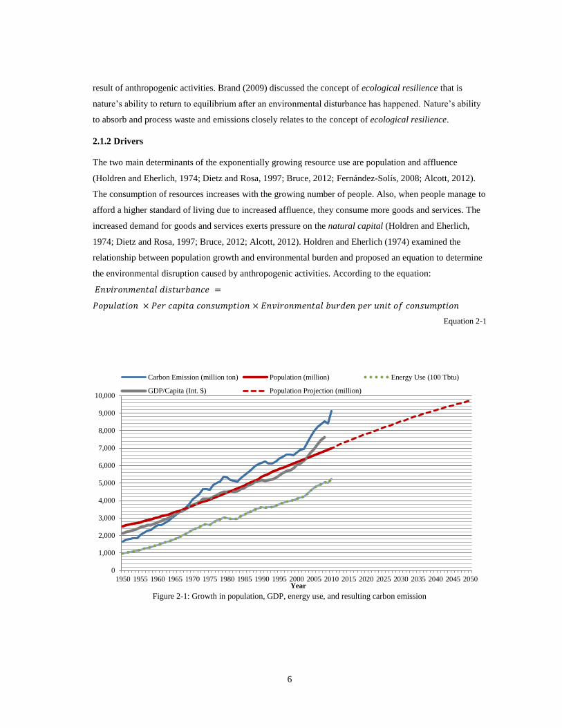
Figure 2-1: Growth in population, GDP, energy use, and resulting carbon emission
0
1,000
2,000
3,000
4,000
5,000
6,000
7,000
8,000
9,000
10,000
1950 1955 1960 1965 1970 1975 1980 1985 1990 1995 2000 2005 2010 2015 2020 2025 2030 2035 2040 2045 2050Year
Carbon Emission (million ton) Population (million) Energy Use (100 Tbtu)
GDP/Capita (Int. $) Population Projection (million)

7
Dietz and Rosa (1997), Bruce (2012), and Alcott (2012) also supported the relationship of environmental
disturbance to population growth and affluence as indicated by the above equation. The equation also
highlights global population and increased affluence as the main drivers of environmental disturbance.
Figure 2-1shows the growth in global population between 1950 and 2010 based on the data sourced from
the United Nation’s Department of Economic and Social Affairs (UNDESA, 2011). It is evident that a
steady growth in global population resulted in an increased energy consumption primarily from fossil fuel
sources. The emission of carbon mainly due to fossil fuel combustion closely followed the energy use
curve. It is interesting to note how a steady growth in per capita Gross Domestic Product (GDP) also
followed the population growth curve closely. A growing GDP indicates an increased demand of goods
and services (a rise in affluence) resulting in mounting emissions as seen in Figure 2-1.
The UNDESA also provided the population projections for the future as shown in Figure 2-1. The global
population, which is over 7 billion currently, is expected to reach 9-10 billion by the end of 2050 (Bruce,
2012; UNDESA, 2011). With nearly 10 billion people on the earth in 2050, one can imagine the grave
situation of resource consumption and emission. The most important aspect of the future global population
is that most of its growth will occur in developing and underdeveloped countries (Bruce, 2012). The
economy of the world’s most populated countries such as India and China is developing at a faster rate and
the affluence level is also increasing (Bruce, 2012; Mendelsohn et al., 2012). Imagine how much resources
would be consumed once the people in these countries attain the same standard of living as the developed
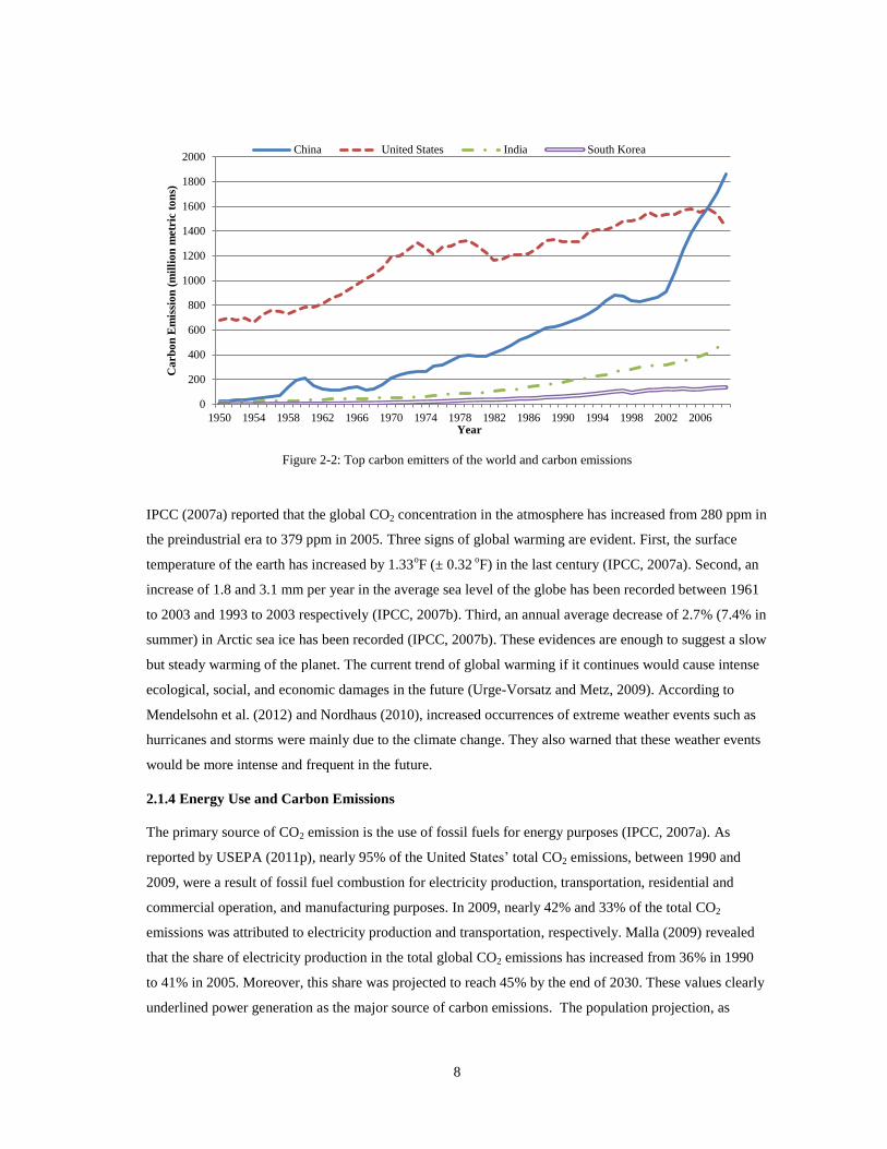
countries (Fernández-Solís, 2008; Bruce, 2012). Figure 2-2 shows the historic carbon emission trends
(1950-2009) for four of the top ten carbon emitters of the world (based on Marland et al., 2010; EPI,
2010). It is scary to see the exponential increase in carbon emission in countries where the maximum
population growth is projected to occur.
2.1.3 Greenhouse Gas Emissions
Among the major impacts of global population increase and rising affluence is the growing concentration
of anthropogenic greenhouse gases (GHG) such as CO2, methane, and nitrous oxide in the atmosphere
(Dietz and Rosa, 1997; Jiang et al., 2008; Alcott, 2012). A fraction of the emitted carbon is absorbed by
the ocean and biomass (e.g. plants) and the remaining fraction is released to the atmosphere in a naturally
occurring carbon cycle. Although the carbon cycle remained mostly balanced in the distant past, after the
industrial revolution a significant rise in CO2 levels (36%) has disturbed its equilibrium (USEPA, 2011p).
One of the major impacts of an increased level of GHG, particularly CO2, in the atmosphere is global
warming leading to the phenomenon of climate change (Nordhaus, 2010; Mendelsohn et al., 2012; Bruce,
2012).
8
Figure 2-2: Top carbon emitters of the world and carbon emissions
IPCC (2007a) reported that the global CO2 concentration in the atmosphere has increased from 280 ppm in
the preindustrial era to 379 ppm in 2005. Three signs of global warming are evident. First, the surface
temperature of the earth has increased by 1.33oF (± 0.32
oF) in the last century (IPCC, 2007a). Second, an
increase of 1.8 and 3.1 mm per year in the average sea level of the globe has been recorded between 1961
to 2003 and 1993 to 2003 respectively (IPCC, 2007b). Third, an annual average decrease of 2.7% (7.4% in
summer) in Arctic sea ice has been recorded (IPCC, 2007b). These evidences are enough to suggest a slow
but steady warming of the planet. The current trend of global warming if it continues would cause intense
ecological, social, and economic damages in the future (Urge-Vorsatz and Metz, 2009). According to
Mendelsohn et al. (2012) and Nordhaus (2010), increased occurrences of extreme weather events such as
hurricanes and storms were mainly due to the climate change. They also warned that these weather events
would be more intense and frequent in the future.
2.1.4 Energy Use and Carbon Emissions
The primary source of CO2 emission is the use of fossil fuels for energy purposes (IPCC, 2007a). As
reported by USEPA (2011p), nearly 95% of the United States’ total CO2 emissions, between 1990 and
2009, were a result of fossil fuel combustion for electricity production, transportation, residential and
commercial operation, and manufacturing purposes. In 2009, nearly 42% and 33% of the total CO2
emissions was attributed to electricity production and transportation, respectively. Malla (2009) revealed
that the share of electricity production in the total global CO2 emissions has increased from 36% in 1990
to 41% in 2005. Moreover, this share was projected to reach 45% by the end of 2030. These values clearly
underlined power generation as the major source of carbon emissions. The population projection, as
0
200
400
600
800
1000
1200
1400
1600
1800
2000
1950 1954 1958 1962 1966 1970 1974 1978 1982 1986 1990 1994 1998 2002 2006
Ca
rb
on
Em
issi
on
(m
illi
on
metr
ic t
on
s)
Year
China United States India South Korea

9
shown in Figure 2-1, clearly demonstrated that with the growing population and affluence, the demand for
electricity and fuel (mostly fossil fuel) would also build up leading to more carbon emissions to the
atmosphere.
How do we address the issue of mounting CO2 concentration in the atmosphere? The answer lies in the
equation proposed by Holdren and Eherlich, (1974). A controlled population growth, optimized per capita
consumption, and improved levels of efficiency in production could bring in significant environmental
benefits. In order to control the current and future rate of environmental degradation, it is critical that a
balance between natural capital consumption and replenishment is gradually restored and the earth’s
ecological resilience is reinforced.
2.2 CONSTRUCTION INDUSTRY AND ENVIRONMENT
2.2.1 Raw Material Consumption
The construction industry is one of the largest consumers of renewable and nonrenewable resources (Palit,
2004; Horvath, 2004; Holtzhausen, 2007; Dixit et al., 2010). It depletes 40% of global energy and 16% of
global water annually. Every year, nearly two-fifths of the global raw stone, sand and gravel supply, and
one-fourth of world’s total virgin wood supply is consumed in construction activities (Ding, 2004;
Langston and Langston, 2008; Dixit et al., 2010). In the United States, between 1975 and 2003, the use of
construction materials such as steel and cement increased by 108 and 57%, respectively (USGS, 2013).
Table 2-1 lists the percent growth in the use of common construction materials in the United States.
According to a study (Matos, 2009) conducted by the United States Geological Survey (USGS), the use of
total raw materials reported in 2006 was over 26 times the consumption in the year 1900. This increase
was 4.7 times more than the growth of the United States’ population in the last century (CSS, 2012).
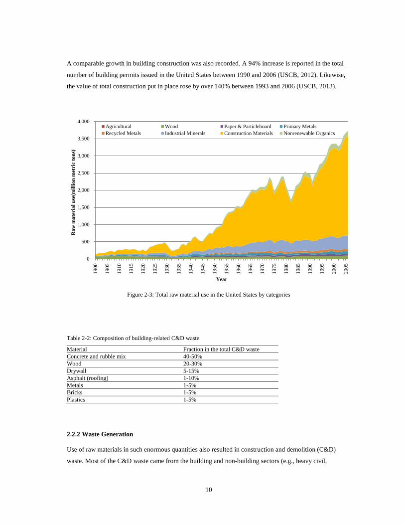
Figure 2-3 illustrates the exponential rise in raw material consumption in the United States in the last 106
years. It is evident that construction materials held the largest share of the total raw material use. It is
interesting to note that the only time the raw material use actually declined was during the events of
adverse economic impacts such as a war, energy crisis, or an economic recession. Nearly 12% of the total
material consumed annually was discharged as trash and 40% was released to the atmosphere (CSS,
2012). Disappointingly, only 5% of the total material consumption was recycled (CSS, 2012).
Table 2-1: Percent increase in the use of common construction materials
Duration Percent Increase in Consumption: United States Construction Industry
Gypsum Aluminum Steel Cement Lime Sand & Gravel Copper
1975-2003 223.0% 12.1% 74.2% 76.8% 114.5% 67.9% 148.9%
1991-2003 107.3% 18.2% 107.7% 56.6% 112.7% 63.8% 33.0%
10
A comparable growth in building construction was also recorded. A 94% increase is reported in the total
number of building permits issued in the United States between 1990 and 2006 (USCB, 2012). Likewise,
the value of total construction put in place rose by over 140% between 1993 and 2006 (USCB, 2013).
Figure 2-3: Total raw material use in the United States by categories
Table 2-2: Composition of building-related C&D waste
Material Fraction in the total C&D waste
Concrete and rubble mix 40-50%
Wood 20-30%
Drywall 5-15%
Asphalt (roofing) 1-10%
Metals 1-5%
Bricks 1-5%
Plastics 1-5%
2.2.2 Waste Generation
Use of raw materials in such enormous quantities also resulted in construction and demolition (C&D)
waste. Most of the C&D waste came from the building and non-building sectors (e.g., heavy civil,
0
500
1,000
1,500
2,000
2,500
3,000
3,500
4,000
19
00
19
05
19
10
19
15
19
20
19
25
19
30
19
35
19
40
19
45
19
50
19
55
19
60
19
65
19
70
19
75
19
80
19
85
19
90
19
95
20
00
20
05
Ra
w m
ate
ria
l u
se(m
illi
on
metr
ic t
on
s)
Year
Agricultural Wood Paper & Particleboard Primary Metals
Recycled Metals Industrial Minerals Construction Materials Nonrenewable Organics
11
transportation, energy). Table 2-2 provides a composition of building-related C&D waste generated each
year (USEPA, 2012).
On an average, a total of 160 million tons of building-related C&D waste is accumulated each year in the
United States (USEPA, 2009a). Approximately half (48%) of the total C&D waste comes from building
demolition activities. Building renovation and new construction activities constitute 44% and 8% of the
total building-related C&D waste, respectively (USEPA, 2009a). Table 2-3 presents the amounts of
building-related C&D waste reported by the USEPA for 1998 and 2003. The yearly estimate of the total
C&D waste was not available, and the USEPA reported estimates for only 1998 and 2003 (Cochran and
Townsend, 2010). Each year roughly 170,000 buildings are constructed and 45,000 buildings are
demolished in the commercial sector (USEPA, 2009a). In the residential sector, nearly 245,000 buildings
are demolished annually (USDOE, 2001). According to an online article by Granger (2009), the total
building and non-building-related C&D waste could add up to 300 million tons each year.
Table 2-3: 1998 and 2003 building-related C&D waste (USEPA, 1998 and 2009b)
Study Year Type of Building Construction (lb/ft2) Renovation (million tons) Demolition (million tons)
1998 Residential 3.89 19.70 31.90
Non-residential 4.27 45.10 28.04
2003 Residential 4.39 19.00 38.00
Non-residential 4.34 65.00 29.00
2.2.3 Greenhouse Gas Emission
The building sector alone is responsible for 33% of the total global carbon emissions (Urge-Vorsatz and
Novikava, 2007; Marszal et al., 2010). In the United States, buildings alone release roughly 39% of the
total CO2 emission 21% of which comes from residential buildings (USEPA, 2009a). Levermore (2008)
reported that, between 1971 and 2002, the annual growth rate in building-related carbon emissions was 1.4
and 2.2% for the residential and commercial sectors, respectively. By the end of 2030, the emissions from
building sector were projected to grow by nearly 72% from its 2002 levels (Levermore, 2008). Most of the
carbon emission released by a building came from fossil fuel combustion. on-site. The total greenhouse
gas emission resulting from a construction site in 2002 was 131 million tons of CO2 equivalent and 100
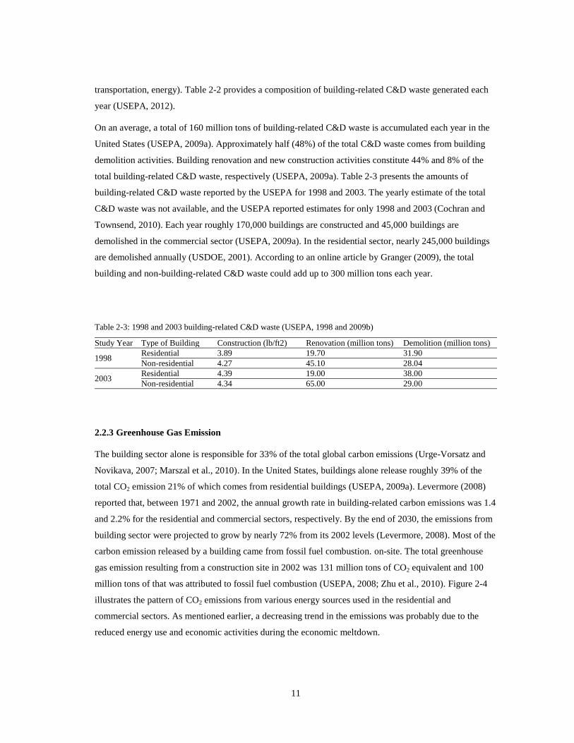
million tons of that was attributed to fossil fuel combustion (USEPA, 2008; Zhu et al., 2010). Figure 2-4
illustrates the pattern of CO2 emissions from various energy sources used in the residential and
commercial sectors. As mentioned earlier, a decreasing trend in the emissions was probably due to the
reduced energy use and economic activities during the economic meltdown.
12
According to the 2002 Economic Census (USCB, 2005), the use of electricity and natural gas in the
United States’ construction industry has increased by 130% and 23%, respectively between 2002 and
2007. As the electric power sector still remains the biggest contributor (33-34%) to the nation’s total CO2
emissions, any increase in electrical demand would raise carbon emission proportionally (USEPA, 2013).
For instance, in 2006, a 2.5% increase in electricity demand resulted in a 3% increase in CO2 emissions
from the electric power sector (USDOE, 2008). Most of the values provided in the literature discussed so
far included emissions resulting from only the direct use of energy (e.g., air-conditioning, lighting,
powering building appliances). The indirect use of energy (e.g. energy of building materials and products)
is seldom included in the calculation of emissions.
Figure 2-4: Carbon emissions from various energy sources
2.3 ENERGY USE IN BUILDINGS
Buildings consume nearly 40% of global energy annually in their life cycle stages of construction, use,
maintenance, and demolition. The energy is consumed by buildings directly or indirectly in a primary
(e.g., natural gas, oil) or delivered (e.g. electricity) form (Dixit et al., 2010; Marszal et al., 2010). In the
United States, the residential structures deplete an average 55% of the total primary energy consumed by
the entire building sector each year (Otto et al., 2010). In the developing countries, the situation of energy
consumption is grave. In China, the residential building sector is responsible for 20-27% of the nation’s
total energy consumption and if the building material production and construction processes are included,
0
200
400
600
800
1000
1200
1400
1600
1800
2000
1973 1980 1990 1996 1998 2000 2002 2004 2006 2008 2010 2012
Ca
rb
on
Dio
xid
e E
mis
sio
n (
mil
lio
n m
etr
ic t
on
s)
Years
Coal Natural Gas Petroleum Electricity
13
this figure reaches up to 37% (Xie, 2011). Gupta (2009) has revealed that the energy consumed in
operating a building in the United Kingdom represented roughly 50% of the nation’s energy. This figure
for a rapidly developing country such as India could be roughly 30% of the total national energy
consumption. However, the situation could turn grave when the percentage of population currently living
in urban areas jumps from 28% to 40% by the end of 2020 (Gupta, 2009). Moreover, the construction
industry in India is currently growing at a 9.2% rate annually, which is nearly two times the global growth
rate of 5.5% (Gupta, 2009).
2.3.1 Life Cycle Energy Components: Embodied and Operating Energy
The total energy consumed by a building over its service life is known as life cycle energy. The total life
cycle energy is composed of two primary components: operating and embodied energy (Treloar, 1998;
Hegner, 2007). During the use phase when the building is occupied, energy sources such as electricity and
natural gas are used in the processes of space conditioning, lighting, and powering building appliances.
This fraction of energy is called operating energy (Crowther, 1999; Hegner, 2007; Dixit et al., 2010).
Electricity and fuels such as oil, natural gas, and coal are also consumed when not only the building but
also its constituent materials are manufactured and delivered. This fraction of energy remains sequestered
in the final product when the product is delivered for the end use. The total energy embedded in all
products and processes that are used in constructing a building is known as embodied energy.
2.3.1.1 Embodied Energy: Definition and Interpretation
Buildings are constructed with a variety of building materials, each of which consumes energy throughout
its life cycle stages of manufacture, use, deconstruction, and disposal. The energy consumed in these
stages is known as the embodied energy of a building material (Vukotic et al., 2010; Dixit et al., 2010).
Similarly, each building also consumes energy during its life cycle stages such as initial construction, use
and maintenance, renovation, demolition, and disposal. Energy is also expended in various administration
and transportation processes during the preconstruction phase. Post construction phases such as
maintenance, renovation, demolition, and disposal also consume energy. The total energy consumed in all
of these life cycle stages is collectively interpreted as the life cycle embodied energy of a building (Cole
and Kernan, 1996; Vukotic et al., 2010).
According to Miller (2001), the term “embodied energy” is subject to numerous interpretations rendered
by different authors and its published measurements are found to be quite unclear. Table 2-4 presents
embodied energy definitions given by various research studies. Studies such as Hegner (2007) and Upton
et al. (2008) defined embodied energy as the nonrenewable fraction of the total embodied energy. Clearly,
current embodied energy definitions represent differences of opinion about the material and energy inputs
to be included in an energy analysis (Hegner, 2007; Nebel, 2007). The embodied energy of a building is
14
made up of two major components: direct energy and indirect energy (Treloar, 1998; Crawford and
Treloar, 2003; Crawford et al., 2006; Khasreen et al., 2009; Dixit et al., 2010).
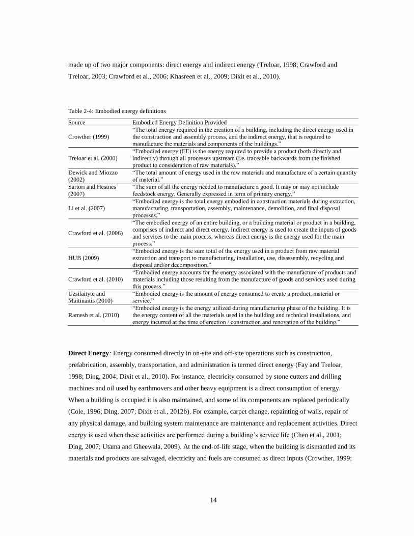
Table 2-4: Embodied energy definitions
Source Embodied Energy Definition Provided
Crowther (1999)
“The total energy required in the creation of a building, including the direct energy used in
the construction and assembly process, and the indirect energy, that is required to
manufacture the materials and components of the buildings.”
Treloar et al. (2000)
“Embodied energy (EE) is the energy required to provide a product (both directly and
indirectly) through all processes upstream (i.e. traceable backwards from the finished
product to consideration of raw materials).”
Dewick and Miozzo
(2002)
“The total amount of energy used in the raw materials and manufacture of a certain quantity
of material.”
Sartori and Hestnes
(2007)
“The sum of all the energy needed to manufacture a good. It may or may not include
feedstock energy. Generally expressed in term of primary energy.”
Li et al. (2007)
“Embodied energy is the total energy embodied in construction materials during extraction,
manufacturing, transportation, assembly, maintenance, demolition, and final disposal
processes.”
Crawford et al. (2006)
“The embodied energy of an entire building, or a building material or product in a building,
comprises of indirect and direct energy. Indirect energy is used to create the inputs of goods
and services to the main process, whereas direct energy is the energy used for the main
process.”
HUB (2009)
“Embodied energy is the sum total of the energy used in a product from raw material
extraction and transport to manufacturing, installation, use, disassembly, recycling and
disposal and/or decomposition.”
Crawford et al. (2010)
“Embodied energy accounts for the energy associated with the manufacture of products and
materials including those resulting from the manufacture of goods and services used during
this process.”
Uzsilaityte and
Maitinaitis (2010)
“Embodied energy is the amount of energy consumed to create a product, material or
service.”
Ramesh et al. (2010)
“Embodied energy is the energy utilized during manufacturing phase of the building. It is
the energy content of all the materials used in the building and technical installations, and
energy incurred at the time of erection / construction and renovation of the building.”
Direct Energy: Energy consumed directly in on-site and off-site operations such as construction,
prefabrication, assembly, transportation, and administration is termed direct energy (Fay and Treloar,
1998; Ding, 2004; Dixit et al., 2010). For instance, electricity consumed by stone cutters and drilling
machines and oil used by earthmovers and other heavy equipment is a direct consumption of energy.
When a building is occupied it is also maintained, and some of its components are replaced periodically
(Cole, 1996; Ding, 2007; Dixit et al., 2012b). For example, carpet change, repainting of walls, repair of
any physical damage, and building system maintenance are maintenance and replacement activities. Direct
energy is used when these activities are performed during a building’s service life (Chen et al., 2001;
Ding, 2007; Utama and Gheewala, 2009). At the end-of-life stage, when the building is dismantled and its
materials and products are salvaged, electricity and fuels are consumed as direct inputs (Crowther, 1999;
15
Miller, 2001; Dixit et al., 2010; Vukotic et al., 2010). All of these energy inputs that are used directly are
categorized as direct energy.
Indirect Energy: Energy used indirectly by a building through nonenergy inputs is known as an indirect
component. For instance, energy spent in manufacturing the building materials, assemblies, and equipment
installed in the buildings is considered an indirect component (Boustead and Hancock, 1978; Treloar,
1998; Crawford, 2004; Dixit et al., 2010; Marszal et al., 2010). A fraction of manufacturing energy of
machines, equipment, and apparatus utilized to manufacture materials is also accounted for as an indirect
energy component (Buchanan and Honey, 1994; Fay, 1999; Hammond and Jones, 2008; Hammond and
Jones, 2010; Dixit et al., 2012a). Major quantities of materials, assemblies, and equipment are mainly
utilized during a building’s initial construction. However, during the use phase, these products may also be
consumed in the processes of maintenance and replacement. Therefore, a considerable portion of the
indirect energy component may be spent during a building’s the use phase (Cole, 1996; Dixit et al., 2013).
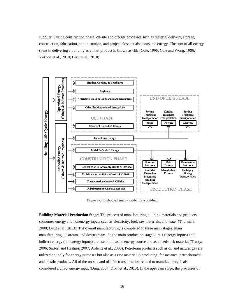
2.3.2 Life Cycle Energy Model
The total life cycle energy used by a building includes direct and indirect components of embodied and
operating energy. This energy use is distributed among three major stages of the life cycle: construction,
use, and end-of-life stage. Figure 2-5 shows an embodied energy model and illustrates the energy use
associated with each of the three stages. The energy used in manufacturing building materials, assemblies,
and equipment and in processes such as construction, installation, fabrication, transportation, and
administration during a building’s construction stage is collectively termed the Initial Embodied Energy
(IEE) (Cole, 1996; Cole and Wong, 1996; Dixit et al., 2010; Vukotic et al., 2010; Dixit et al., 2013). The
Recurrent Embodied Energy (REE) includes energy used in maintenance and replacement activities during
the use phase of a built facility. At the end of its service life, when a facility is demolished and its
materials are transported for reuse, recycling, and disposal, the total energy consumed is known as
Demolition Energy (DE) (Cole, 1996; Cole and Wong, 1996; Dixit et al., 2010; Vukotic et al., 2010; Dixit
et al., 2013). The total life cycle embodied energy (LCEE) of a building is the sum of its initial, recurrent,
and demolition energy. The total life cycle energy (LCE) of a built facility includes LCEE and operating
energy (OE) (Cole, 1996; Cole and Wong, 1996; Dixit et al., 2010; Vukotic et al., 2010; Dixit et al., 2013).
2.3.2.1 Initial Embodied Energy (IEE)
The IEE is composed of the total energy used during the building material production and building
construction phase (Cole, 1996; Cole and Wong, 1996; Vukotic et al., 2010; Dixit et al., 2010). In the
material production phase, the upstream processes such as raw material extraction, treatment, and
transportation to production unit are quite energy intensive. The main production process involves use of
both the electricity and fuels. Fuels are used both as an energy source and as a feedstock material. In the
downstream, energy is expended when the final product is delivered to a construction site or a material
16
supplier. During construction phase, on-site and off-site processes such as material delivery, storage,
construction, fabrication, administration, and project closeout also consume energy. The sum of all energy
spent in delivering a building as a final product is known as IEE (Cole, 1996; Cole and Wong, 1996;
Vukotic et al., 2010; Dixit et al., 2010).
Figure 2-5: Embodied energy model for a building
Building Material Production Stage: The process of manufacturing building materials and products
consumes energy and nonenergy inputs such as electricity, fuel, raw materials, and water (Thormark,
2000; Dixit et al., 2013). The overall manufacturing is completed in three main stages: main
manufacturing, upstream, and downstream. In the main production stage, direct (energy inputs) and
indirect energy (nonenergy inputs) are used both as an energy source and as a feedstock material (Trusty,
2006; Sartori and Hestnes, 2007; Ardente et al., 2008). Petroleum products such as oil and natural gas are
utilized not only for energy purposes but also as a raw material in producing, for instance, petrochemical
and plastic products. All of the on-site and off-site transportation related to manufacturing is also
considered a direct energy input (Ding, 2004; Dixit et al., 2013). In the upstream stage, the processes of
17
raw material extraction, treatment, handling, storage, and transportation to the manufacturing unit also
deplete energy and nonenergy sources that are counted as well (Cole, 1996; Ding, 2004; Vukotic et al.,
2010). In the downstream of the main production process, when a finished product is packaged, labeled,
stored, and transported to a construction site or a material supplier, energy is consumed directly and
indirectly (Cole, 1996; Cole and Wong, 1996; Ding, 2004; Dixit et al., 2013). In some cases, the delivery
of finished building materials to their destination could be quite energy intensive depending on the
distance and mode of transport (Ding, 2004).
The sum of all energy used up directly and indirectly in the main production, upstream, and downstream
processes until the final product reaches its destination is considered building materials’ production
energy. The energy of material production represents the largest share of a building’s total LCEE (Chen et
al., 2001; Scheuer et al., 2003; Vukotic et al., 2010). In an analysis of two high-rise residential buildings in
Hong Kong, Chen et al. (2001) concluded that the manufacturing energy shared up to 90-92% of a
building’s total LCEE. In a similar study of a six-story university building done by Scheuer et al. (2003),
the total energy embodied in material production was found to be nearly 94% of the total LCEE
(excluding construction and transportation). In Sweden, a study by Adalberth (1997b) found that nearly
64-65% of the total LCEE (over 50 years’ service life) of three prefabricated single-family dwellings came
from building materials’ production. Similarly, Leckner & Zmeureanu (2011) studied a base case and a
net-zero energy version of a two-floor house in Canada and found the share of building materials as 70%
of the total LCEE over 40 years’ service life. They used embodied energy data from Athena Impact
Estimator developed by the Athena Sustainable Materials Institute. The proportions of building material
manufacturing energy in the total LCEE calculated by Chen et al. (2001) and Scheuer et al. (2003) are
higher than the ones calculated by Adalberth (1997b) and Leckner and Zmeureanu (2011). The value
calculated by Scheuer et al. (2003) also included building materials used during replacement and
maintenance processes over 75 years’ service life, whereas Chen et al. (2001) did not include building
systems in the maintenance and replacement phase. As mentioned earlier, the most commonly-used
materials such as aluminum, steel, and plastics have a higher embodied energy. Table 2-5 shows the
energy embodied in some of the commonly used building materials. Building materials such as cement
(7.8 MJ/kg), glass (16-17 MJ/kg), plastics (70 MJ/kg), and insulation materials (16-105 MJ/kg) are quite
energy intensive and contribute significantly to a building’s IEE (Chen et al., 2001; Dimoudi and Tompa,
2008).
It can be seen that there is a considerable variation in the reported values of embodied energy. Energy
intensive materials such as aluminum and polystyrene insulation have a wider embodied energy range of
130-379 MJ/kg and 58-116 MJ/kg, respectively. The embodied energy of one of the most widely used
materials such as timber, ranged from 1.7-22.6 MJ/kg. According to Dixit et al. (2010), the embodied
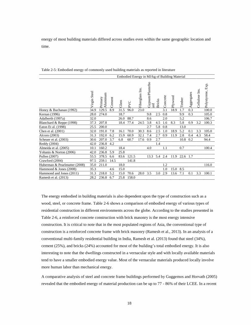
18
energy of most building materials differed across studies even within the same geographic location and
time.
Table 2-5: Embodied energy of commonly used building materials as reported in literature
Embodied Energy in MJ/kg of Building Material
Vir
gin
Ste
el
Pri
mar
y
Alu
min
um
Cem
ent
Gla
ss
PV
C
Fib
erg
lass
Ins.
Gy
psu
m/P
last
erbo
ard
Bri
cks
Co
ncr
ete
Ply
woo
d
Tim
ber
Ag
gre
gat
es
Cel
lulo
se I
ns.
Poly
styre
ne,
Exp
.
Honey & Buchanan (1992) 34.9 129.5 8.9 31.5 96.0 23.0
3.1 18.9 1.7 0.3
100.0
Kernan (1996) 28.0 274.0
18.7
9.8 2.5 0.8
9.9 0.3
105.0
Adalberth (1997a) 32.0
26.0 88.7
8.6
2.0
5.2
106.7
Blanchard & Reppe (1998) 37.3 207.8
18.4 77.4 24.5 3.8 4.5 1.6 8.3 5.8 0.9 3.2 100.3
Eaton Et al. (1998) 25.5 200.0
2.7 5.8 0.8
13.0
Chen et al. (2001) 32.0 191.0 7.8 16.1 70.0 30.3 8.6 2.5 1.0 18.9 5.2 0.1 3.3 105.0
Alcorn (2003) 31.3 192.0 6.2 15.9 60.9 32.1 7.4 2.7 0.9 11.9 2.8 0.4 4.3 58.4
Scheuer et al. (2003) 30.6 207.0 3.7 6.8 60.7 17.6 0.9 2.7
10.8 0.2
94.4
Reddy (2004) 42.0 236.8 4.2
1.4
Almeida et al. (2005) 10.1 160.2 18.4 4.0 1.1 0.7 100.4
Yohanis & Norton (2006) 42.0 236.8 5.9 25.8
Pullen (2007) 55.5 378.5 6.6 83.6 121.5
13.3 5.4 2.4 11.9 22.6 1.7
Crawford (2004) 97.5 259.1 14.5
141.8
Huberman & Pearlmutter (2008) 35.0 211.0
18.0
1.2
116.0
Hammond & Jones (2008) 35.3 4.6 15.0 1.0 15.0 8.5
Hammond and Jones (2011) 31.3 218.0 5.2 15.0 70.6 28.0 3.5 3.0 2.9 13.6 7.1 0.1 3.3 100.1
Ramesh et al. (2013) 28.2 236.8 6.7 25.8 158.0
The energy embodied in building materials is also dependent upon the type of construction such as a
wood, steel, or concrete frame. Table 2-6 shows a comparison of embodied energy of various types of
residential construction in different environments across the globe. According to the studies presented in
Table 2-6, a reinforced concrete construction with brick masonry is the most energy intensive
construction. It is critical to note that in the most populated regions of Asia, the conventional type of
construction is a reinforced concrete frame with brick masonry (Ramesh et al., 2013). In an analysis of a
conventional multi-family residential building in India, Ramesh et al. (2013) found that steel (34%),
cement (25%), and bricks (24%) accounted for most of the building’s total embodied energy. It is also
interesting to note that the dwellings constructed in a vernacular style and with locally available materials
tend to have a smaller embodied energy value. Most of the vernacular materials produced locally involve
more human labor than mechanical energy.
A comparative analysis of steel and concrete frame buildings performed by Guggemos and Horvath (2005)
revealed that the embodied energy of material production can be up to 77 - 86% of their LCEE. In a recent
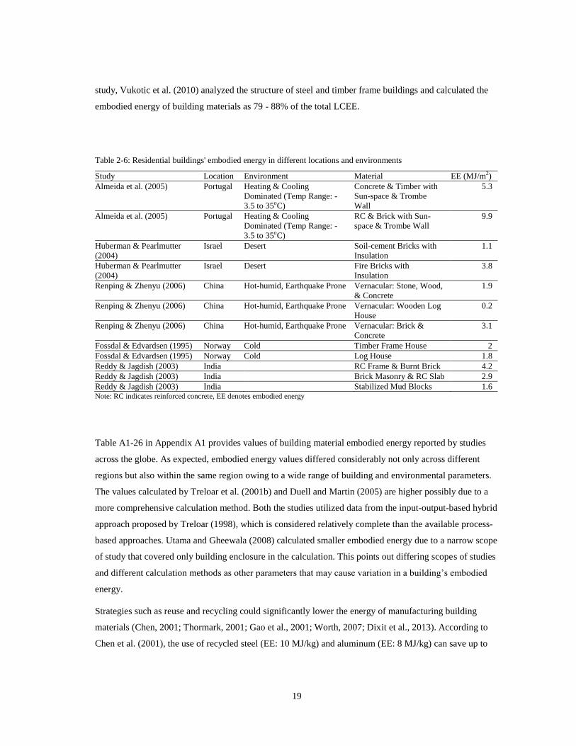
19
study, Vukotic et al. (2010) analyzed the structure of steel and timber frame buildings and calculated the
embodied energy of building materials as 79 - 88% of the total LCEE.
Table 2-6: Residential buildings' embodied energy in different locations and environments
Study Location Environment Material EE (MJ/m2)
Almeida et al. (2005) Portugal Heating & Cooling
Dominated (Temp Range: -
3.5 to 35oC)
Concrete & Timber with
Sun-space & Trombe
Wall
5.3
Almeida et al. (2005) Portugal Heating & Cooling
Dominated (Temp Range: -
3.5 to 35oC)
RC & Brick with Sun-
space & Trombe Wall
9.9
Huberman & Pearlmutter
(2004)
Israel Desert Soil-cement Bricks with
Insulation
1.1
Huberman & Pearlmutter
(2004)
Israel Desert Fire Bricks with
Insulation
3.8
Renping & Zhenyu (2006) China Hot-humid, Earthquake Prone Vernacular: Stone, Wood,
& Concrete
1.9
Renping & Zhenyu (2006) China Hot-humid, Earthquake Prone Vernacular: Wooden Log
House
0.2
Renping & Zhenyu (2006) China Hot-humid, Earthquake Prone Vernacular: Brick &
Concrete
3.1
Fossdal & Edvardsen (1995) Norway Cold Timber Frame House 2
Fossdal & Edvardsen (1995) Norway Cold Log House 1.8
Reddy & Jagdish (2003) India RC Frame & Burnt Brick 4.2
Reddy & Jagdish (2003) India Brick Masonry & RC Slab 2.9
Reddy & Jagdish (2003) India Stabilized Mud Blocks 1.6 Note: RC indicates reinforced concrete, EE denotes embodied energy
Table A1-26 in Appendix A1 provides values of building material embodied energy reported by studies
across the globe. As expected, embodied energy values differed considerably not only across different
regions but also within the same region owing to a wide range of building and environmental parameters.
The values calculated by Treloar et al. (2001b) and Duell and Martin (2005) are higher possibly due to a
more comprehensive calculation method. Both the studies utilized data from the input-output-based hybrid
approach proposed by Treloar (1998), which is considered relatively complete than the available process-
based approaches. Utama and Gheewala (2008) calculated smaller embodied energy due to a narrow scope
of study that covered only building enclosure in the calculation. This points out differing scopes of studies
and different calculation methods as other parameters that may cause variation in a building’s embodied
energy.
Strategies such as reuse and recycling could significantly lower the energy of manufacturing building
materials (Chen, 2001; Thormark, 2001; Gao et al., 2001; Worth, 2007; Dixit et al., 2013). According to
Chen et al. (2001), the use of recycled steel (EE: 10 MJ/kg) and aluminum (EE: 8 MJ/kg) can save up to
20
70 - 96% of the manufacturing energy of virgin steel (EE: 32 MJ/kg) and primary aluminum (EE: 191
MJ/kg). Two types of recycling occur at this stage. A material can be recycled through a postconsumer or
pre-consumer recycling. A postconsumer recycling involves obtaining a recycled material from a source
external to the industry meaning the material is recycled after a consumer has already used it. Such a
recycling across industries is also known as what Treloar et al. (2003) and Thormark (2002) have defined,
an open loop recycling. In the pre-consumer recycling, recycled materials are sourced within the
manufacturing industry. In this case, the material has not reached its final consumer before being recycled.
Pre-consumer recycling is also termed closed loop recycling (Thormark, 2002; Treloar, 2003; Meil et al.,
2004). At least 60% of the total manufacturing energy can be conserved by using recycled materials (Chen
et al., 2001).
Transportation Energy: The finished building materials are transported from the manufacturing unit to a
construction site or material supplier, which may be located in the same country or overseas. Hence,
building materials could be distributed locally, imported from a foreign country, or exported to other
locations involving a variety of transportation modes and consuming a wide range of energy sources
(Peuportier, 2001; Chen et al., 2001; Miller, 2001; Lucuik et al., 2006). Building materials and products
may be hauled to their point of use by surface (road and rail), water (boats and ships), or air transportation
depending on the destination (Peuportier, 2001; Chen et al., 2001). According to Fay (1999), the energy
used by sea vessels may be just 10% of the energy used in air transportation. Studies such as Chen et al.
(2001) reported that energy use in domestic surface transportation of building material could be negligible,
whereas exporting or importing building products could be very energy intensive. However, in an analysis
of a modular home, Kim (2008) found that the energy consumed in domestic transportation of materials
was nearly 8% of its total embodied energy. Peuportier (2001) questioned whether a return trip should be
counted in the calculation, particularly in the case of a one-way trip delivery, as it is most likely that the
delivery vehicle (e.g. trucks) may return empty. Eventually, only half of the return distance was included,
as chances of trains and ships returning empty are highly unlikely. Miller (2001) reported that if the return
distance and road infrastructure are considered, the energy embodied in transporting building materials
may increase drastically.
The fraction of energy embodied in material transport is widely debated in the literature. Fay (1999) cited
Miller (1996) who determined that the transportation energy consumed in a building was roughly 6% of
the total LCEE. Later, Miller (2001) determined that the transportation energy was 1 - 1.5% of the total
life cycle embedded energy (based on published data) and it could increase if the energy of return trips,
vehicle manufacture, construction of roads, and other transport infrastructure were included. Whether to
include the indirect fraction of energy associated with the transport infrastructure, automobile production,
and labor in the transport energy calculation is still a contentious issue. Chen et al. (2001) found a larger
value of transportation energy (7% of the LCEE) due to inclusion of surface and sea transportation of
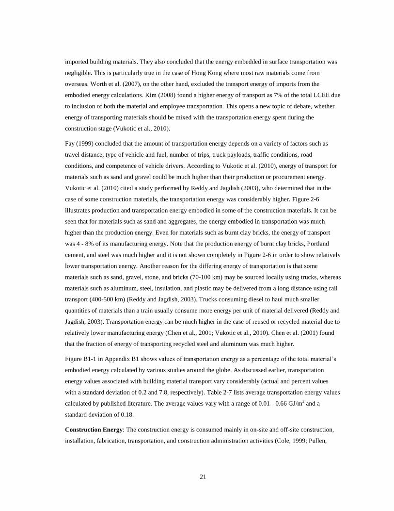
21
imported building materials. They also concluded that the energy embedded in surface transportation was
negligible. This is particularly true in the case of Hong Kong where most raw materials come from
overseas. Worth et al. (2007), on the other hand, excluded the transport energy of imports from the
embodied energy calculations. Kim (2008) found a higher energy of transport as 7% of the total LCEE due
to inclusion of both the material and employee transportation. This opens a new topic of debate, whether
energy of transporting materials should be mixed with the transportation energy spent during the
construction stage (Vukotic et al., 2010).
Fay (1999) concluded that the amount of transportation energy depends on a variety of factors such as
travel distance, type of vehicle and fuel, number of trips, truck payloads, traffic conditions, road
conditions, and competence of vehicle drivers. According to Vukotic et al. (2010), energy of transport for
materials such as sand and gravel could be much higher than their production or procurement energy.
Vukotic et al. (2010) cited a study performed by Reddy and Jagdish (2003), who determined that in the
case of some construction materials, the transportation energy was considerably higher. Figure 2-6
illustrates production and transportation energy embodied in some of the construction materials. It can be
seen that for materials such as sand and aggregates, the energy embodied in transportation was much
higher than the production energy. Even for materials such as burnt clay bricks, the energy of transport
was 4 - 8% of its manufacturing energy. Note that the production energy of burnt clay bricks, Portland
cement, and steel was much higher and it is not shown completely in Figure 2-6 in order to show relatively
lower transportation energy. Another reason for the differing energy of transportation is that some
materials such as sand, gravel, stone, and bricks (70-100 km) may be sourced locally using trucks, whereas
materials such as aluminum, steel, insulation, and plastic may be delivered from a long distance using rail
transport (400-500 km) (Reddy and Jagdish, 2003). Trucks consuming diesel to haul much smaller
quantities of materials than a train usually consume more energy per unit of material delivered (Reddy and
Jagdish, 2003). Transportation energy can be much higher in the case of reused or recycled material due to
relatively lower manufacturing energy (Chen et al., 2001; Vukotic et al., 2010). Chen et al. (2001) found
that the fraction of energy of transporting recycled steel and aluminum was much higher.
Figure B1-1 in Appendix B1 shows values of transportation energy as a percentage of the total material’s
embodied energy calculated by various studies around the globe. As discussed earlier, transportation
energy values associated with building material transport vary considerably (actual and percent values
with a standard deviation of 0.2 and 7.8, respectively). Table 2-7 lists average transportation energy values
calculated by published literature. The average values vary with a range of 0.01 - 0.66 GJ/m2 and a
standard deviation of 0.18.
Construction Energy: The construction energy is consumed mainly in on-site and off-site construction,
installation, fabrication, transportation, and construction administration activities (Cole, 1999; Pullen,
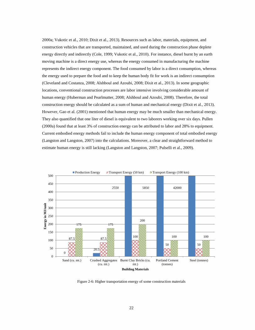
22
2000a; Vukotic et al., 2010; Dixit et al., 2013). Resources such as labor, materials, equipment, and
construction vehicles that are transported, maintained, and used during the construction phase deplete
energy directly and indirectly (Cole, 1999; Vukotic et al., 2010). For instance, diesel burnt by an earth
moving machine is a direct energy use, whereas the energy consumed in manufacturing the machine
represents the indirect energy component. The food consumed by labor is a direct consumption, whereas
the energy used to prepare the food and to keep the human body fit for work is an indirect consumption
(Cleveland and Costanza, 2008; Alshboul and Azoubi, 2008; Dixit et al., 2013). In some geographic
locations, conventional construction processes are labor intensive involving considerable amount of
human energy (Huberman and Pearlmutter, 2008; Alshboul and Azoubi, 2008). Therefore, the total
construction energy should be calculated as a sum of human and mechanical energy (Dixit et al., 2013).
However, Gao et al. (2001) mentioned that human energy may be much smaller than mechanical energy.
They also quantified that one liter of diesel is equivalent to two laborers working over six days. Pullen
(2000a) found that at least 3% of construction energy can be attributed to labor and 28% to equipment.
Current embodied energy methods fail to include the human energy component of total embodied energy
(Langston and Langston, 2007) into the calculations. Moreover, a clear and straightforward method to
estimate human energy is still lacking (Langston and Langston, 2007; Pulselli et al., 2009).
Figure 2-6: Higher transportation energy of some construction materials
0 20.5
87.5 87.5 100
50 50
175 175
200
100 100
0
50
100
150
200
250
300
350
400
450
500
Sand (cu. mt.) Crushed Aggregates
(cu. mt.)
Burnt Clay Bricks (cu.
mt.)
Portland Cement
(tonnes)
Steel (tonnes)
En
erg
y in
MJ
/un
it
Building Materials
Production Energy Transport Energy (50 km) Transport Energy (100 km)
2550 5850 42000
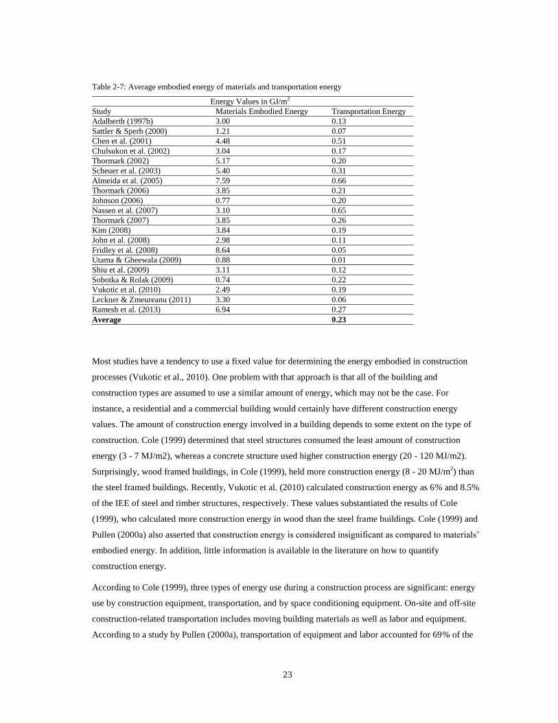
23
Table 2-7: Average embodied energy of materials and transportation energy
Energy Values in GJ/m2
Study Materials Embodied Energy Transportation Energy
Adalberth (1997b) 3.00 0.13
Sattler & Sperb (2000) 1.21 0.07
Chen et al. (2001) 4.48 0.51
Chulsukon et al. (2002) 3.04 0.17
Thormark (2002) 5.17 0.20
Scheuer et al. (2003) 5.40 0.31
Almeida et al. (2005) 7.59 0.66
Thormark (2006) 3.85 0.21
Johnson (2006) 0.77 0.20
Nassen et al. (2007) 3.10 0.65
Thormark (2007) 3.85 0.26
Kim (2008) 3.84 0.19
John et al. (2008) 2.98 0.11
Fridley et al. (2008) 8.64 0.05
Utama & Gheewala (2009) 0.88 0.01
Shiu et al. (2009) 3.11 0.12
Sobotka & Rolak (2009) 0.74 0.22
Vukotic et al. (2010) 2.49 0.19
Leckner & Zmeureanu (2011) 3.30 0.06
Ramesh et al. (2013) 6.94 0.27
Average 0.23
Most studies have a tendency to use a fixed value for determining the energy embodied in construction
processes (Vukotic et al., 2010). One problem with that approach is that all of the building and
construction types are assumed to use a similar amount of energy, which may not be the case. For
instance, a residential and a commercial building would certainly have different construction energy
values. The amount of construction energy involved in a building depends to some extent on the type of
construction. Cole (1999) determined that steel structures consumed the least amount of construction
energy (3 - 7 MJ/m2), whereas a concrete structure used higher construction energy (20 - 120 MJ/m2).
Surprisingly, wood framed buildings, in Cole (1999), held more construction energy (8 - 20 MJ/m2) than
the steel framed buildings. Recently, Vukotic et al. (2010) calculated construction energy as 6% and 8.5%
of the IEE of steel and timber structures, respectively. These values substantiated the results of Cole
(1999), who calculated more construction energy in wood than the steel frame buildings. Cole (1999) and
Pullen (2000a) also asserted that construction energy is considered insignificant as compared to materials’
embodied energy. In addition, little information is available in the literature on how to quantify
construction energy.
According to Cole (1999), three types of energy use during a construction process are significant: energy
use by construction equipment, transportation, and by space conditioning equipment. On-site and off-site
construction-related transportation includes moving building materials as well as labor and equipment.
According to a study by Pullen (2000a), transportation of equipment and labor accounted for 69% of the

24
total construction energy. Construction workers and administrative staff commute to construction sites and
other places such as regional and corporate offices using mostly individual or sometimes shared vehicles
(Cole, 1999). Heavy and light construction equipment such as cranes, loaders, and forklifts are also moved
during the course of construction. Usually, the transportation of workers involves the use of gasoline,
whereas moving and operating heavy equipment consumes fuels such as diesel. Fay (1999) cited studies
by Stein et al. (1981), Baird et al. (1983) and Viljoen (1995), which determined the construction energy
within a range of 6 - 17% of the total LCEE. In a similar study, Pullen (2000a) referred to studies by
Ballantyne (1980), Lord (1994), and Lawson (1996) who found the construction energy within the range
of 7 - 15% of the total LCEE. Cole (1999) included transportation of heavy equipment and workers in the
calculation and found higher construction energy (7 - 10% of IEE). Much like Cole (1999), Vukotic et al.
(2010) also counted the transportation of materials and labor during the materials’ production and
construction stages.
Figure 2-7 shows the average values of construction energy in various types of construction reported by
studies mentioned in Table 2-8. Table 2-8 provides the average values of materials’ embodied energy and
construction energy reported in the literature. The average results in Figure 2-7 further support the findings
of Cole (1999) and Vukotic et al. (2010) that the steel frame buildings required less construction energy
than the wood frame. In addition, concrete frame is the most energy intensive type of construction.
Increased need of labor, equipment, and formwork for concrete construction may be among the possible
reasons for its higher energy requirement. The average reported values ranged from 0.01 - 1.18 GJ/m2 and
varied with a standard deviation of 0.34.
A large amount of waste is generated when building materials are moved, installed, and transformed
during the construction process (Chen et al., 2001; Treloar et al., 2003). Energy embedded indirectly in
construction waste could be significant, and would be lost if not recovered by reuse and recycling
(Vukotic et al., 2010; Treloar et al., 2003). Construction waste may be hazardous and may also carry
adverse environmental impacts if not handled properly. The amount of waste generated in the construction
processes depends on a waste factor, which is the percentage of a material that may be wasted during the
material’s use (Worth et al., 2007; Treloar et al., 2003; Adalberth, 1997b; Blengini, 2009). Studies have
derived different waste factors for different building materials. Table 2-9 presents the waste factors
calculated by various studies. Materials can also be reused in the construction process without changing
their current forms (Chen et al., 2001; Thormark, 2001). Building products that are made of materials such
as wood and metals can be reused for the same or different purposes. The C&D debris that includes mostly
concrete and brick can be reused as gravel in the construction of buildings (Thormark, 2001).
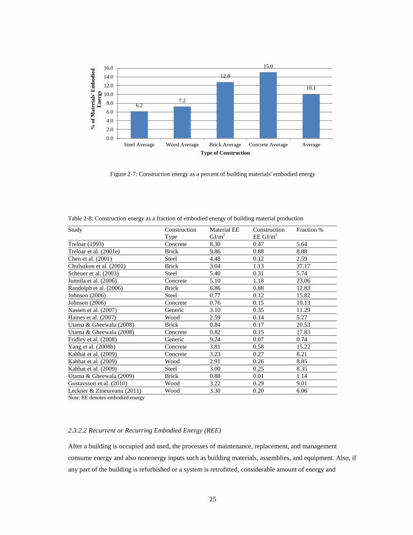
25
Figure 2-7: Construction energy as a percent of building materials' embodied energy
Table 2-8: Construction energy as a fraction of embodied energy of building material production
Study Construction
Type
Material EE
GJ/m2
Construction
EE GJ/m2
Fraction %
Treloar (1993) Concrete 8.30 0.47 5.64
Treloar et al. (2001e) Brick 9.86 0.88 8.88
Chen et al. (2001) Steel 4.48 0.12 2.59
Chulsukon et al. (2002) Brick 3.04 1.13 37.17
Scheuer et al. (2003) Steel 5.40 0.31 5.74
Junnila et al. (2006) Concrete 5.10 1.18 23.06
Randolph et al. (2006) Brick 6.86 0.88 12.83
Johnson (2006) Steel 0.77 0.12 15.82
Johnson (2006) Concrete 0.76 0.15 19.13
Nassen et al. (2007) Generic 3.10 0.35 11.29
Haines et al. (2007) Wood 2.59 0.14 5.27
Utama & Gheewala (2008) Brick 0.84 0.17 20.53
Utama & Gheewala (2008) Concrete 0.82 0.15 17.83
Fridley et al. (2008) Generic 9.24 0.07 0.74
Yang et al. (2008b) Concrete 3.81 0.58 15.22
Kahhat et al. (2009) Concrete 3.23 0.27 8.21
Kahhat et al. (2009) Wood 2.91 0.26 8.85
Kahhat et al. (2009) Steel 3.00 0.25 8.35
Utama & Gheewala (2009) Brick 0.88 0.01 1.14
Gustavsson et al. (2010) Wood 3.22 0.29 9.01
Leckner & Zmeureanu (2011) Wood 3.30 0.20 6.06 Note: EE denotes embodied energy
2.3.2.2 Recurrent or Recurring Embodied Energy (REE)
After a building is occupied and used, the processes of maintenance, replacement, and management
consume energy and also nonenergy inputs such as building materials, assemblies, and equipment. Also, if
any part of the building is refurbished or a system is retrofitted, considerable amount of energy and
6.2 7.2
12.8
15.0
10.1
0.0
2.0
4.0
6.0
8.0
10.0
12.0
14.0
16.0
Steel Average Wood Average Brick Average Concrete Average Average
% o
f M
ate
ria
ls' E
mb
od
ied
En
erg
y
Type of Construction
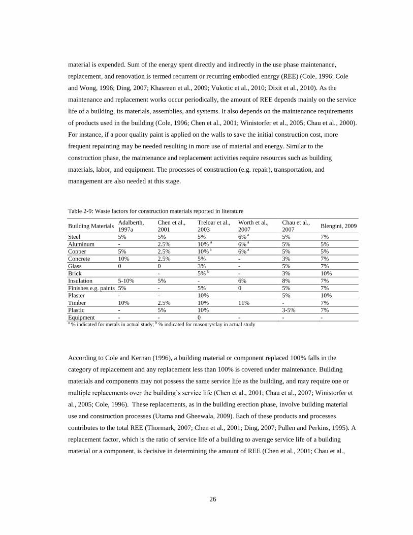
26
material is expended. Sum of the energy spent directly and indirectly in the use phase maintenance,
replacement, and renovation is termed recurrent or recurring embodied energy (REE) (Cole, 1996; Cole
and Wong, 1996; Ding, 2007; Khasreen et al., 2009; Vukotic et al., 2010; Dixit et al., 2010). As the
maintenance and replacement works occur periodically, the amount of REE depends mainly on the service
life of a building, its materials, assemblies, and systems. It also depends on the maintenance requirements
of products used in the building (Cole, 1996; Chen et al., 2001; Winistorfer et al., 2005; Chau et al., 2000).
For instance, if a poor quality paint is applied on the walls to save the initial construction cost, more
frequent repainting may be needed resulting in more use of material and energy. Similar to the
construction phase, the maintenance and replacement activities require resources such as building
materials, labor, and equipment. The processes of construction (e.g. repair), transportation, and
management are also needed at this stage.
Table 2-9: Waste factors for construction materials reported in literature
Building Materials Adalberth,
1997a
Chen et al.,
2001
Treloar et al.,
2003
Worth et al.,
2007
Chau et al.,
2007 Blengini, 2009
Steel 5% 5% 5% 6% a 5% 7%
Aluminum - 2.5% 10% a 6% a 5% 5%
Copper 5% 2.5% 10% a 6% a 5% 5%
Concrete 10% 2.5% 5% - 3% 7%
Glass 0 0 3% - 5% 7%
Brick - 5% b - 3% 10%
Insulation 5-10% 5% - 6% 8% 7%
Finishes e.g. paints 5% - 5% 0 5% 7%
Plaster - - 10% 5% 10%
Timber 10% 2.5% 10% 11% - 7%
Plastic - 5% 10% 3-5% 7%
Equipment - - 0 - - - a % indicated for metals in actual study; b % indicated for masonry/clay in actual study
According to Cole and Kernan (1996), a building material or component replaced 100% falls in the
category of replacement and any replacement less than 100% is covered under maintenance. Building
materials and components may not possess the same service life as the building, and may require one or
multiple replacements over the building’s service life (Chen et al., 2001; Chau et al., 2007; Winistorfer et
al., 2005; Cole, 1996). These replacements, as in the building erection phase, involve building material
use and construction processes (Utama and Gheewala, 2009). Each of these products and processes
contributes to the total REE (Thormark, 2007; Chen et al., 2001; Ding, 2007; Pullen and Perkins, 1995). A
replacement factor, which is the ratio of service life of a building to average service life of a building
material or a component, is decisive in determining the amount of REE (Chen et al., 2001; Chau et al.,
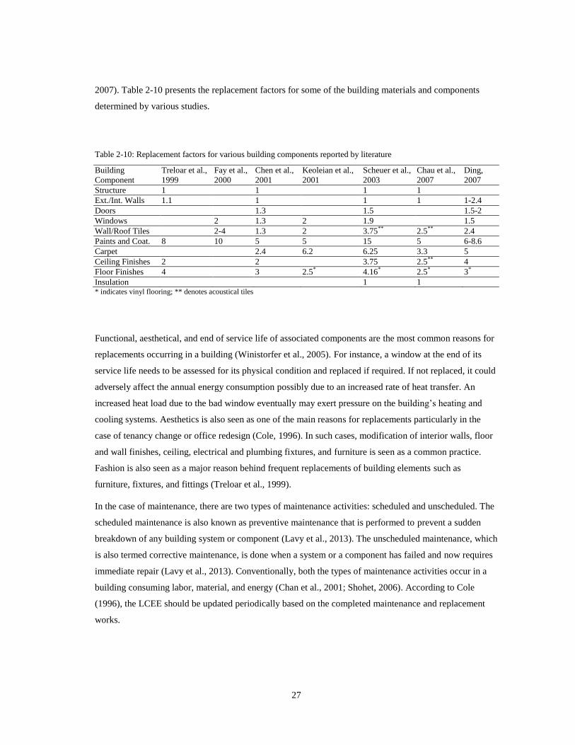
27
2007). Table 2-10 presents the replacement factors for some of the building materials and components
determined by various studies.
Table 2-10: Replacement factors for various building components reported by literature
Building
Component
Treloar et al.,
1999
Fay et al.,
2000
Chen et al.,
2001
Keoleian et al.,
2001
Scheuer et al.,
2003
Chau et al.,
2007
Ding,
2007
Structure 1 1 1 1
Ext./Int. Walls 1.1 1 1 1 1-2.4
Doors 1.3 1.5 1.5-2
Windows 2 1.3 2 1.9 1.5
Wall/Roof Tiles 2-4 1.3 2 3.75** 2.5** 2.4
Paints and Coat. 8 10 5 5 15 5 6-8.6
Carpet 2.4 6.2 6.25 3.3 5
Ceiling Finishes 2 2 3.75 2.5** 4
Floor Finishes 4 3 2.5* 4.16* 2.5* 3*
Insulation 1 1 * indicates vinyl flooring; ** denotes acoustical tiles
Functional, aesthetical, and end of service life of associated components are the most common reasons for
replacements occurring in a building (Winistorfer et al., 2005). For instance, a window at the end of its
service life needs to be assessed for its physical condition and replaced if required. If not replaced, it could
adversely affect the annual energy consumption possibly due to an increased rate of heat transfer. An
increased heat load due to the bad window eventually may exert pressure on the building’s heating and
cooling systems. Aesthetics is also seen as one of the main reasons for replacements particularly in the
case of tenancy change or office redesign (Cole, 1996). In such cases, modification of interior walls, floor
and wall finishes, ceiling, electrical and plumbing fixtures, and furniture is seen as a common practice.
Fashion is also seen as a major reason behind frequent replacements of building elements such as
furniture, fixtures, and fittings (Treloar et al., 1999).
In the case of maintenance, there are two types of maintenance activities: scheduled and unscheduled. The
scheduled maintenance is also known as preventive maintenance that is performed to prevent a sudden
breakdown of any building system or component (Lavy et al., 2013). The unscheduled maintenance, which
is also termed corrective maintenance, is done when a system or a component has failed and now requires
immediate repair (Lavy et al., 2013). Conventionally, both the types of maintenance activities occur in a
building consuming labor, material, and energy (Chan et al., 2001; Shohet, 2006). According to Cole
(1996), the LCEE should be updated periodically based on the completed maintenance and replacement
works.
28
In 50 years of service life, a building’s REE could equalize its IEE (Cole, 1996). In the case of Australian
Secondary Schools, Ding (2007) found that the REE, over a 60-year service life, was 72% of the school
buildings’ total LCEE. Building components such as envelope, finishes, and services, which may not hold
higher embodied energy initially, require a significant recurring energy (3.2 times the initial embodied
energy in a 50-year service life) (Cole, 1996). Similarly, Cole (1996) determined that for a service life of
25, 50, and 100 years, the REE of these components was 1.3, 3.2, and 7.3 times their IEE, respectively.
Treloar et al. (2000) and Adalberth (1997b) calculated recurring embodied energy as 45% (50-year service
life) and 32% (30-year service life) of IEE, respectively. Pullen (2000a) determined an annual REE of 1%
of the total IEE. This value is in accordance with the values suggested by Adalberth (1997b) and Treloar et
al. (2000). In a study of 15 houses in the Adelaide region of Australia, Pullen and Perkins (1995) found the
recurring embodied energy (for an 80-year service life) within a range of 36 - 84% of the total IEE
(average 57%).
A building’s REE increases with its service life. Factors such as durability, long service life, low
maintenance requirements, functional suitability, and recycling and reuse potential of products installed in
a building could significantly lower the amount of REE (Dixit et al., 2012b). Dixit et al. (2012b)
conducted a rigorous analysis of 64 single and multi-family residential and 100 commercial case studies
published in the literature. As buildings had differing service lives, for a fair comparison, REE values were
annualized and expressed in MJ/m2/year (Dixit et al., 2012b). In the case of residential buildings, Dixit et
al. (2012b) found a moderate and positive correlation of REE with the buildings’ service life (r2 = 0.50)
but a strong positive correlation with their total LCEE (r2 = 0.94) and LCE (r
2 = 0.73). Figure B1-2 and
Figure B1-3 in Appendix B1 illustrate the correlation of REE with the buildings’ total LCE and LCEE,
respectively. This means that the REE influences the LCE and LCEE more than any other life cycle
embodied energy component. In the case of commercial buildings, the correlation of REE with the total
LCEE (r2 = 0.96) and LCE (r
2 = 0.83) was very strong and positive indicating a strong influence of REE
over LCEE. The correlation of commercial buildings’ REE with their service life was moderate and
positive (r2 = 0.68). According to Dixit et al. (2012b), the residential buildings conventionally do not
involve very complex, modernized, and large size building systems and components requiring a greater
degree of maintenance and replacements (Scheuer et al., 2003). This may be one of the reasons why REE
of residential buildings showed a weaker correlation than the commercial buildings (Dixit et al., 2013).
Figure B1-4 in Appendix B1shows the variations in the reported values of REE. The annual REE
requirements for the residential buildings vary from 8 to 213 MJ/m2/year with an average of
62.3MJ/m2/year. The REE values calculated by Barnes and Rankin (1975) were the lowest among the
referred residential facilities. One reason for this may be the fixed percentage (0.9% of IEE) considered
calculating the REE in the study. Fay and Treloar (1998) calculated a higher REE value (188 - 213
MJ/m2/year) due to the inclusion of maintenance and replacement requirements for not only the building
29
and its components but also the landscaping and major building appliances (stove, microwave oven,
dishwasher, clothes washer and dryer, heater etc.). The REE values ranged from 1.7 to 470 MJ/m2/year for
commercial facilities with an average REE value of 157 MJ/m2/year. The lower annual REE values (1.7 -
3.6 MJ/m2/year) calculated by Page (2006) are due to the fact that only exterior walls and roof paint were
included under the maintenance and replacement works. The annual REE values reported by Langston and
Langston (2007) were significantly higher (up to 470 MJ/m2/year), as they included the building, its
components, services, fittings, site works and external services. They, like Fay and Treloar (1998), also
used the input-output-based hybrid method to calculate the energy embodied, which usually results in
higher energy values (Crawford et al., 2002).
2.3.2.3 Demolition Energy (DE)
At the end of its service life, a building is demolished and its constituent materials are sorted, treated, and
transported for reuse, recycling, or disposal to landfills or incinerators. Both the electricity and fuel are
consumed directly and indirectly in the demolition and disposal processes. The sum of total energy
consumed is termed demolition energy (DE) (Cole, 1996; Cole and Wong, 1996; Vukotic et al., 2010;
Dixit et al., 2010). Energy is consumed in four stages at the end-of-life phase of a building. The first stage
involves complete demolition and disassembly of the building, and utilizes heavy equipment such as
hydraulic hammers and hydraulic loaders consuming fuels such as oil (Miller, 2001; Blengini, 2009). In
the second stage, on-site secondary demolition occurs, the purpose of which is to separate building
materials and reduce their size for easy handling and sorting. Waste as well as salvaged materials are then
transported to either landfills or to reuse and recycling facilities in the third stage. Finally, equipment such
as jaw crushers and magnetic separators are used to separate and salvage reusable and recyclable materials
at the recycling facilities. Sorted reusable or recyclable materials are then transported to manufacturing
facilities or construction sites by means of trucks and trains (Blengini, 2009). One important activity at this
stage includes recycling and reuse processes that could recover a major fraction of initial energy embodied
in the building (Crowther, 1999; Tingley et al., 2012). Recycling and reuse may be an open loop or a
closed loop type process (Tingley et al., 2012). In an open loop materials are recycled or reused between
industries or life cycle stages of a building, whereas closed loop involves recycling and reuse within the
same industry or life cycle stage (Thormark, 2002; Treloar et al., 2003).
Studies (e.g., Cole and Kernan, 1996; Scheuer et al., 2003; Adalberth, 1997b; Kernan, 1996; Kofoworola
and Gheewala, 2009; Shu-hua et al., 2010) performed detailed life cycle assessment of buildings and
derived a percentage of IEE that could be used for demolition energy calculation. Adalberth (1997b) and
Cole and Kernan (1996) calculated the demolition energy as 4% and 1 - 3% of a building’s total IEE,
respectively. Scheuer et al. (2003) reported a higher demolition energy that was 12% of the total IEE of
the study building. This higher value was probably due to the inclusion of the decommissioning of all
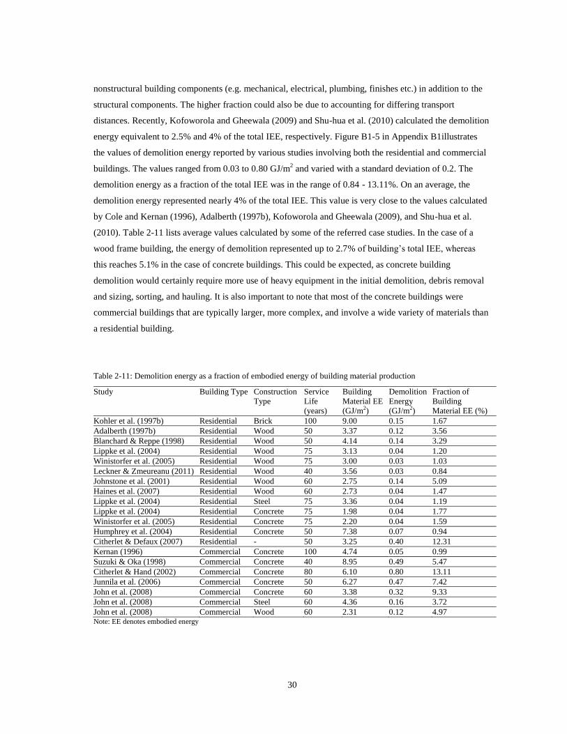
30
nonstructural building components (e.g. mechanical, electrical, plumbing, finishes etc.) in addition to the
structural components. The higher fraction could also be due to accounting for differing transport
distances. Recently, Kofoworola and Gheewala (2009) and Shu-hua et al. (2010) calculated the demolition
energy equivalent to 2.5% and 4% of the total IEE, respectively. Figure B1-5 in Appendix B1illustrates
the values of demolition energy reported by various studies involving both the residential and commercial
buildings. The values ranged from 0.03 to 0.80 GJ/m2 and varied with a standard deviation of 0.2. The
demolition energy as a fraction of the total IEE was in the range of 0.84 - 13.11%. On an average, the
demolition energy represented nearly 4% of the total IEE. This value is very close to the values calculated
by Cole and Kernan (1996), Adalberth (1997b), Kofoworola and Gheewala (2009), and Shu-hua et al.
(2010). Table 2-11 lists average values calculated by some of the referred case studies. In the case of a
wood frame building, the energy of demolition represented up to 2.7% of building’s total IEE, whereas
this reaches 5.1% in the case of concrete buildings. This could be expected, as concrete building
demolition would certainly require more use of heavy equipment in the initial demolition, debris removal
and sizing, sorting, and hauling. It is also important to note that most of the concrete buildings were
commercial buildings that are typically larger, more complex, and involve a wide variety of materials than
a residential building.
Table 2-11: Demolition energy as a fraction of embodied energy of building material production
Study Building Type Construction
Type
Service
Life
(years)
Building
Material EE
(GJ/m2)
Demolition
Energy
(GJ/m2)
Fraction of
Building
Material EE (%)
Kohler et al. (1997b) Residential Brick 100 9.00 0.15 1.67
Adalberth (1997b) Residential Wood 50 3.37 0.12 3.56
Blanchard & Reppe (1998) Residential Wood 50 4.14 0.14 3.29
Lippke et al. (2004) Residential Wood 75 3.13 0.04 1.20
Winistorfer et al. (2005) Residential Wood 75 3.00 0.03 1.03
Leckner & Zmeureanu (2011) Residential Wood 40 3.56 0.03 0.84
Johnstone et al. (2001) Residential Wood 60 2.75 0.14 5.09
Haines et al. (2007) Residential Wood 60 2.73 0.04 1.47
Lippke et al. (2004) Residential Steel 75 3.36 0.04 1.19
Lippke et al. (2004) Residential Concrete 75 1.98 0.04 1.77
Winistorfer et al. (2005) Residential Concrete 75 2.20 0.04 1.59
Humphrey et al. (2004) Residential Concrete 50 7.38 0.07 0.94
Citherlet & Defaux (2007) Residential - 50 3.25 0.40 12.31
Kernan (1996) Commercial Concrete 100 4.74 0.05 0.99
Suzuki & Oka (1998) Commercial Concrete 40 8.95 0.49 5.47
Citherlet & Hand (2002) Commercial Concrete 80 6.10 0.80 13.11
Junnila et al. (2006) Commercial Concrete 50 6.27 0.47 7.42
John et al. (2008) Commercial Concrete 60 3.38 0.32 9.33
John et al. (2008) Commercial Steel 60 4.36 0.16 3.72
John et al. (2008) Commercial Wood 60 2.31 0.12 4.97 Note: EE denotes embodied energy

31
ACHP (1979) proposed a demolition energy figure of 136.3 MJ/m2 for a 5000 m
2 concrete building. These
energy values accounted for 1 - 3% of IEE as demolition energy (Cole and Wong, 1996; Cole and Kernan,
1996). Table 2-11 provides the demolition energy values presented by ACHP (1979).
2.3.3 Life Cycle Embodied Energy Components: Reported Values
Among the three major life cycle embodied energy components are initial embodied energy (IEE),
recurrent embodied energy (REE), and demolition energy (DE). Among them, according to the reported
results in the literature, the most influential energy components are REE and IEE. As discussed earlier, the
REE showed a strong and positive correlation to a building’s LCEE and LCE. This section of the literature
review discusses and synthesizes various studies and their results in order to derive a range of proportions
each component shares in the total LCEE. A rigorous review of literature was performed that included
embodied energy case studies from 1976 through 2011.
Figure 2-8 shows the breakup of IEE, REE, and DE in total LCEE reported by case studies that calculated
all three components. The variation in the proportions of the energy components is due to the presence of
both the residential and commercial type of buildings with brick, wood, steel, and concrete construction.
Table A1-1, Table A1-2, Table A1-3, and Table A1-4 in Appendix A1 provide the life cycle energy
breakup in terms of total IEE, REE, OE, and DE for brick, concrete, steel, and wood frame buildings. In
the tables, IEE, REE, OE, and DE denote initial embodied energy, recurrent embodied energy, operating
energy, and demolition energy, respectively.
In the case of brick construction, the average value of REE was nearly half of the IEE values. It can be
seen that for a 100 years’ service life, a building’s REE could be over 1.5 times its IEE as calculated by
Kohler et al. (1997). This further supports the notion that REE and LCEE are dependent on a building’s
service life. In the case of concrete construction, the annualized REE values calculated by Cole and
Kernan (1996), Kernan (1996), Eaton et al. (1998), Citherlet and Hands (2002), and Humphrey et al.
(2004) were considerably higher (1.3 - 1.6 times) than IEE. In the case of brick buildings, the average REE
was 46% of the buildings’ IEE and it increased to 61% for concrete buildings. Similarly in the case of
wood and steel frame buildings, the REE calculated by Jacques (1996), Cole and Kernan (1996), and
Eaton et al. (1998) easily surpassed the IEE values within a service span of 50 - 60 years.
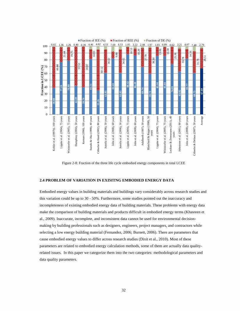
32
Figure 2-8: Fraction of the three life cycle embodied energy components in total LCEE
2.4 PROBLEM OF VARIATION IN EXISITNG EMBODIED ENERGY DATA
Embodied energy values in building materials and buildings vary considerably across research studies and
this variation could be up to 30 - 50%. Furthermore, some studies pointed out the inaccuracy and
incompleteness of existing embodied energy data of building materials. These problems with energy data
make the comparison of building materials and products difficult in embodied energy terms (Khasreen et
al., 2009). Inaccurate, incomplete, and inconsistent data cannot be used for environmental decision-
making by building professionals such as designers, engineers, project managers, and contractors while
selecting a low energy building material (Fernandez, 2006; Burnett, 2006). There are parameters that
cause embodied energy values to differ across research studies (Dixit et al., 2010). Most of these
parameters are related to embodied energy calculation methods, some of them are actually data quality-
related issues. In this paper we categorize them into the two categories: methodological parameters and
data quality parameters.
38.8
8
77.1
9
78.9
9
42.0
9
39.7
4
81.5
1
35.2
6
61.0
5 8
2.4
3
61.0
5
88.4
2
86.4
9
69.7
4
59.7
3
85.9
1
85.8
1
74.0
1
63.0
2 8
1.7
7
60.7
5
67.6
9
60.4
8
21.4
4
19.7
5
57.5
2
59.8
7
14.0
3
60.1
2
34.4
2 9
.88
34.4
2
10.5
3
10.2
9
27.7
8
38.3
0
13.0
6
13.3
0
25.3
6
33.7
8 14.1
6
31.7
8
29.5
1
0.65 1.36 1.26 0.40 0.39 4.46 4.62 4.53 7.69 4.53 1.05 3.22 2.48 1.97 1.03 0.89 0.62 3.21 4.07 7.48 2.79
0
10
20
30
40
50
60
70
80
90
100
Ko
hle
r et
al.
(1
99
7b
), 1
00
yea
rs
Lip
pk
e et
al.
(2
00
4),
75
yea
rs
Win
isto
rfer
et
al. (2
00
5),
75
yea
rs
Hu
mp
hre
y (
20
04
), 5
0 y
ears
Ker
nan
(1
99
6),
10
0 y
ears
Su
zuk
i &
Ok
a (1
99
8),
40
yea
rs
Cit
her
let
& H
and
(2
00
2),
80
yea
rs
Jun
nil
a et
al.
(2
00
6),
50
yea
rs
Joh
n e
t al
. (2
00
8),
60
yea
rs
Jun
nil
a et
al.
(2
00
6),
50
yea
rs
Lip
pk
e et
al.
(2
00
4),
75
yea
rs
Joh
n e
t al
. (2
00
8),
60
yea
rs
Ad
alb
erth
(1
99
7),
50
yea
rs
Bla
nch
ard
& R
epp
e (1
99
8),
50
yea
rs
Lip
pk
e et
al.
(2
00
4),
75
yea
rs
Win
isto
rfer
et
al. (2
00
5),
75
yea
rs
Lec
kn
er &
Zm
eure
anu
(2
01
1),
40
yea
rs
Joh
nst
on
e et
al.
(2
00
1),
60
yea
rs
Joh
n e
t al
. (2
00
8),
60
yea
rs
Cit
her
let
& D
efau
x (
20
07
), 5
0 y
ears
Av
erag
e
Fra
cti
on
in
LC
EE
(%
) Fraction of IEE (%) Fraction of REE (%) Fraction of DE (%)

33
2.4.1 Methodological Parameters
Parameters such as system boundary, methods of embodied energy measurement, and type and form of
energy to be included relate closely to embodied energy calculation methodology.
2.4.1.1 System Boundary: Problem of Incompleteness
The system boundary demarcates a system of various products and processes related to the manufacturing
of a product under study. A system boundary also determines the number and type of energy and material
inputs included in the calculation of embodied energy (IFIAS, 1975; Peuportier, 2001). Miller (2001) and
Khasreen et al. (2009) asserted that research studies often do not describe the system boundary adopted in
their study clearly and it becomes difficult for the readers to determine what is included and excluded from
the energy calculation. Suh et al. (2004) stated that studies often select the system boundary of the energy
analysis subjectively and results of such studies cannot be compared. Raynolds et al. (2000) emphasized
the need for a system that ensures consistent system boundary selection across different studies. System
boundary definition differs across studies, which leads to variations in the calculated embodied energy
values (Dixit et al., 2010).
2.4.1.2 Method of Embodied Energy Calculation
Among the major embodied energy calculation methods are input-output-based, process-based, hybrid and
statistical analysis (Fay and Treloar, 1998; Lenzen, 2000; Crawford and Treloar, 2003; Ding, 2004; Plank,
2008; Khasreen et al., 2009; Optis and Wild, 2010). Each of these methods has limitations and varying
levels of accuracy. Consequently, results of these methods differ and affect their comparative evaluation
(Miller, 2001; Crawford and Treloar, 2005; Nassen et al., 2007; Plank, 2008; Khasreen et al., 2009; Optis
and Wild, 2010). Another method that is called hybrid analysis includes both the process and the input-
output data and is considered relatively complete and accurate. Research studies have applied different
calculation methods and their embodied energy results differ significantly (Nebel, 2007; Dixit et al.,
2010).
Nassen et al. (2007) performed a detailed analysis of input-output and process-based energy calculation
methods and found that the results of an input-output-based analysis could be 90% higher than a process-
based analysis. Crawford and Treloar (2003) calculated embodied energy in a residential and a
commercial building as 6.6 GJ/m2 and 9.0 GJ/m
2, respectively using a process-based analysis.
Furthermore, they also found that embodied energy in the same buildings could decrease by 14.5 - 23% if
an input-output-based analysis is used. Crawford and Treloar (2005) later studied a commercial building
and concluded that when an input-output-based calculation was performed, the calculated values increased
by 56% from the building’s process-based values (8.0 GJ/m2). Optis and Wild (2010) concluded that
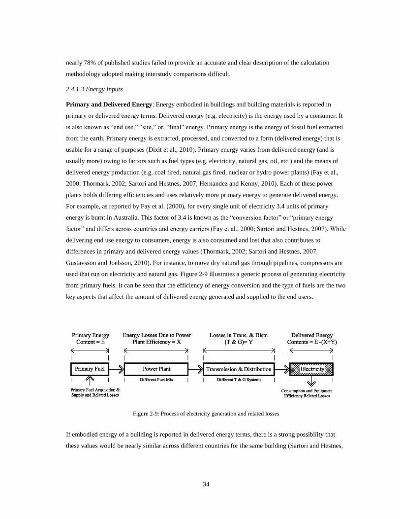
34
nearly 78% of published studies failed to provide an accurate and clear description of the calculation
methodology adopted making interstudy comparisons difficult.
2.4.1.3 Energy Inputs
Primary and Delivered Energy: Energy embodied in buildings and building materials is reported in
primary or delivered energy terms. Delivered energy (e.g. electricity) is the energy used by a consumer. It
is also known as “end use,” “site,” or, “final” energy. Primary energy is the energy of fossil fuel extracted
from the earth. Primary energy is extracted, processed, and converted to a form (delivered energy) that is
usable for a range of purposes (Dixit et al., 2010). Primary energy varies from delivered energy (and is
usually more) owing to factors such as fuel types (e.g. electricity, natural gas, oil, etc.) and the means of
delivered energy production (e.g. coal fired, natural gas fired, nuclear or hydro power plants) (Fay et al.,
2000; Thormark, 2002; Sartori and Hestnes, 2007; Hernandez and Kenny, 2010). Each of these power
plants holds differing efficiencies and uses relatively more primary energy to generate delivered energy.
For example, as reported by Fay et al. (2000), for every single unit of electricity 3.4 units of primary
energy is burnt in Australia. This factor of 3.4 is known as the “conversion factor” or “primary energy
factor” and differs across countries and energy carriers (Fay et al., 2000; Sartori and Hestnes, 2007). While
delivering end use energy to consumers, energy is also consumed and lost that also contributes to
differences in primary and delivered energy values (Thormark, 2002; Sartori and Hestnes, 2007;
Gustavsson and Joelsson, 2010). For instance, to move dry natural gas through pipelines, compressors are
used that run on electricity and natural gas. Figure 2-9 illustrates a generic process of generating electricity
from primary fuels. It can be seen that the efficiency of energy conversion and the type of fuels are the two
key aspects that affect the amount of delivered energy generated and supplied to the end users.
Figure 2-9: Process of electricity generation and related losses
If embodied energy of a building is reported in delivered energy terms, there is a strong possibility that
these values would be nearly similar across different countries for the same building (Sartori and Hestnes,
35
2007). Such data cannot be compared globally, as the actual amount of primary energy consumed and true
environmental impacts remain covered under delivered energy values (Fay and Treloar, 1998; Thormark,
2002; Sartori and Hestnes, 2007). Embodied energy presented in primary energy terms can portray a true
picture of environmental burden, as primary energy values could provide a relatively accurate estimate of
resulting greenhouse gas emissions (Pullen, 2007; Fridley et al., 2008; Gustavsson and Joelsson, 2010;
Hernandez and Kenny, 2010). Studies have reported energy embodied in buildings and building materials
either in a primary or delivered energy term or have not provided any indication of the energy term
(Sartori and Hestnes, 2007; Gustavsson and Joelsson, 2010; Ramesh et al., 2010). Results of such studies
differ considerably and cannot be compared. Pears (1996) revealed that embodied energy values could
increase by 30 - 40% (from delivered energy term) if reported in a primary energy form.
Feedstock Energy: ISO 14040 (2006) defined feedstock energy as “heat of combustion of a raw material
input that is not used as an energy source to a product system, expressed in terms of higher heating value
or lower heating value.” Feedstock energy is the heat of combustion or energy content of raw material
input (e.g. wood and petrochemicals, such as oil and gas) used as ingredient in the process of
manufacturing a product (e.g. wood components, plastics and rubber) (Trusty, 2006; Sartori and Hestnes,
2007; Ardente et al., 2008).
Embodied energy includes feedstock energy and the nonrenewable fraction of all direct and indirect
energies consumed in manufacturing a product (Lucuik et al., 2006; Hegner, 2007; Krogmann et al., 2008;
ASMI, 2009). Research studies have concluded that the feedstock energy could constitute a major fraction
of the total embodied energy. Sartori and Hestnes (2007) argued that the embodied energy may or may not
include the feedstock energy. However, studies such as Thormark (2002 and 2006), Lucuik et al. (2006),
Trusty (2006), Ardente et al. (2008), Blengini (2009) and Gustavsson et al. (2010) accommodated
feedstock energy into the total embodied energy calculations. Some of these studies (Thormark, 2002;
Trusty, 2006; Thormark, 2007; Ardente et al., 2008) have presented the values of feedstock energy
separately to highlight their importance. Thormark (2001) and (2007) found the feedstock energy as 27 -
94% of the materials’ embodied energy (released materials). Ardente et al. (2008) conducted a “cradle to
gate” LCA of the Kenaf-fiber insulation boards and revealed that nearly 50% of the total embodied energy
was attributed to the material’s feedstock. In a similar study, Lazzarin et al. (2008) quantified the
feedstock energy of stone wool, expanded polystyrene foam, expanded polyurethane foam, and cork
panels as 16%, 48%, 59%, and 88% of the material’s total embodied energy, respectively. The feedstock
component is the largest contributor to the total energy embodied in construction materials such as asphalt
(Trusty, 2006).
Feedstock energy is significant and hence, needs to be considered in the embodied energy calculation
(Thormark, 2006; Nassen et al., 2007; Ardente et al., 2008; Hammond and Jones, 2008 and 2010).
36
Inclusion or exclusion of feedstock energy in embodied energy calculation could cause variations in
embodied energy values (Pullen, 2000b; Nassen et al., 2007). Nassen et al. (2007) noted that calculation
methods such as input-output-based analyses do not accommodate feedstock energy of raw material
inputs. Furthermore, they had to exclude feedstock energy values from total embodied energy values
rendered by referred studies in order to make genuine comparisons in their study.
Nonrenewable Energy: Hegner (2007) presented an interesting explanation of embodied energy, citing
Kasser and Poll (1998). According to them, only energy that is available in a limited amount should be
considered embodied energy. Here, they relate the phenomenon of embodied energy to greenhouse gas
emissions because a major fraction of primary energy available in a limited amount comes from fossil
fuels. Recent studies (Citherlet and Hand, 2002; Holtzhausen, 2007; Upton et al., 2008; Fernandez, 2008;
Verbeeck and Hens, 2010; De Meester et al., 2009; Pittet and Kotak, 2009; Black et al., 2010; Aste et al.,
2010; Leckner and Zmeureanu, 2011) presented their energy results separately in nonrenewable energy
terms to emphasize the environmental significance of embodied energy as an evaluation parameter.
Studies (Hegner, 2007; Joseph and Tretsiakova-McNally, 2010; Ramesh et al., 2010) also claimed that
embodied energy (in nonrenewable terms) becomes a vital environmental indicator of the greenhouse gas
emission impacts of manufacturing a product.
Human Energy: In some geographic locations, conventional manufacturing processes of building
materials and certain construction processes are labor intensive and involve considerable amount of human
energy (Huberman and Pearlmutter, 2008; Alshboul and Alzoubi, 2008; Utama and Gheewala, 2008).
Langston and Langston (2007) noted that some of the building’s life cycle activities such as maintenance
and repair are more labor intensive than the initial construction and this fraction of human energy is often
excluded from the embodied energy analysis. Studies (Langston and Langston, 2007; Pulselli et al., 2009)
underscored a need to incorporate human energy in embodied energy analysis. However, it is often not
accomplished due to the lack of a clear human energy calculation method. Dias and Pooliyadda (2004)
discussed the importance of human energy but could not accommodate it in their calculations owing to the
complexity and ambiguity involved in its analysis.
One significant study that calculated human energy was done by Alshboul and Alzoubi (2008) who
performed embodied energy analysis of the natural-dimensioned stone in Jordan. They measured human
energy using work duration and metabolic rates. However, they found that the variability of individual
metabolic rates poses difficulty in consistently calculating the human energy. Another important work by
Cleveland and Costanza (2008) discussed human labor and identified three components, which should be
accounted for while quantifying the human energy. These are: 1. the calorific value of food consumed by
workers, 2. the embodied energy of food, and 3. fuel purchased with salaries or wages of workers.
37
Current embodied energy methods fail to include the human energy component of total embodied energy
(Langston and Langston, 2007; Ulgiati et al., 2010). In developed countries such as the United States, a
significant amount of energy is consumed in growing, harvesting, transporting, marketing, storing, and
preparing human food (Cleveland and Costanza, 2008). Grondzik et al. (2009) noted that some building
materials are more human energy intensive than others that consume more mechanical energy. This further
adds to the variability of materials’ embodied energy.
2.4.2 Data Quality Parameters
Data quality is one of the key parameters, which differ within and across databases (Szaley and Nebel,
2006; Optis and Wild, 2010). Ardente et al. (2011) discussed a Data Quality Index (DQI) to determine the
quality of data on the basis of age and representativeness of data. Quality of data used governs the
reliability of energy analysis (Menzies et al., 2007; Khasreen et al., 2009). According to Optis and Wild
(2010), about 20% of the studies do not mention data sources clearly, making it difficult for researchers to
use or analyze their results. The following factors affect the quality of data used in an energy analysis:
2.4.2.1 Primary and Secondary Data
Khasreen et al. (2009) and Crawford and Treloar (2005) argued that the success or failure of an embodied
energy analysis depends upon the quality and source of the data referred. Studies applied different
techniques to acquire data. Some studies utilized primary data sources such as economic input-output
tables, process data, and datasets attached to software, whereas some sourced secondary data from other
published studies (Dixit et al., 2010). Goggins et al. (2010) claimed that the accuracy of embodied energy
data depends upon the methods of embodied energy measurement. Often, embodied energy is also
calculated using Life Cycle Assessment (LCA) tools and datasets such as Athena, BEES 4.0, Ecoinvent,
Eco-Quantum, Envest 2, OPTIMIZE, LICHEE, and SimaPro. However, some of these tools do not cover
all stages of a building’s life cycle and lack the capability to perform a full life cycle assessment (Ting,
2006; Itard, 2007; Haapio and Viitaniemi, 2008; Khasreen, 2009). Plank (2008) also warned that most of
these available tools act as a “black box”, as they lack transparency and flexibility. According to
Hammond and Jones (2008), if it is difficult to discern the system boundary adopted by the secondary data
sources, such data should not be trusted.
2.4.2.2 Data Incompleteness
According to Menzies et al. (2007) and Peereboom et al. (1998), research studies often do not have access
to primary data sources and rely on secondary data sources that may or may not be complete. The
incompleteness of data stems from either the lack of data, limitations of the calculation methods, or a
subjective selection of system boundaries (Menzies et al., 2007; Reap et al., 2008; Goggins et al., 2010;
Monahan and Powel, 2010). Studies that performed embodied energy calculations based on process
38
analysis often suffered from data incompleteness, as accounting for nearly all processes would have been a
difficult task (Menzies et al., 2010; Hammond and Jones, 2010; Goggins et al., 2010). As a result, process
analysis outcomes are underestimated and include data gaps (Menzies et al., 2007; Hammond and Jones,
2010). Existing LCA and embodied energy inventories are seriously incomplete and poor in data quality
(Reap et al., 2008; Khasreen et al., 2009). Researchers ignore, assume, or estimate missing data whenever
they encounter data gaps in the inventory and often end up inferring data from the literature (Reap et al.,
2008; Monahan and Powel, 2010). Data incompleteness should be verified when choosing one material
dataset over another (Alcorn, 1996; Crawford et al., 2006; Nebel, 2007; Khasreen et al., 2009).
2.4.2.3 Data Representativeness
Data representativeness is an important quality, which if lacking could make data irrelevant to the study
and could change the direction of the analysis (Pittet and Kotak, 2009; Khasreen et al., 2009; Optis and
Wild, 2010). Most of the current LCA studies used data that did not represent the local conditions
(Huberman and Pearlmutter, 2008). According to literature, data should have the following
representativeness:
Geographical Representativeness: Geographic relevance of data is the only factor causing the largest
variation in LCA or embodied energy results (Khasreen et al., 2009; Optis and Wild, 2010). Countries
around the globe differ in terms of use of construction materials, construction and fabrication processes,
mode of transportation, and transportation distances (Menzies et al., 2007; Pittet and Kotak, 2009; Rule et
al., 2009; Goggins et al., 2010). Moreover, the technology of construction material production and
construction also differs in terms of efficiency (Menzies et al., 2007; Pittet and Kotak, 2009; Goggins et
al., 2010). The fuel and technology used for electricity production, electricity mix (renewable and
nonrenewable), and economic systems vary significantly around the globe (Sartori and Hestnes, 2007;
Menzies et al., 2007; Monahan and Powell, 2010; Hammond and Jones, 2010). According to Buchanan
and Honey (1994), differing energy supply assumptions could cause embodied energy and carbon results
to vary by a factor of three. Energy tariffs paid by material manufacturers and material prices are also
different in various locations causing an error up to 2.5% in the calculations (Pullen, 1996).
Temporal Representativeness: Studies often apply data that is obsolete and lacks temporal representation
(Reap et al., 2008). In a paper focused on energy embodied in historic buildings, Frey (2008) discussed
that old and outdated data should not be used directly for current situations. If possible, data should be
modified to suit the current time. Studies based on input-output analysis often lacked the temporal
relevance, as the analysis was based upon economic input-output tables, which most countries do not
publish in a timely manner (Menzies et al., 2007). Technology of electricity production as well as
construction material manufacturing could change over time and old data, if used, may not represent the
39
study in current time (Buchanan and Honey, 1994; Pullen, 2000b; Crawford and Treloar, 2005; Menzies et
al., 2007).
Technological Representativeness: Different technologies of material manufacture consume a varied
amount of energy, as the new advanced technologies are relatively more efficient than the older ones. A
downward trend was also observed in the energy consumption of process energy involved in construction
material manufacturing (Menzies et al., 2007). This indicates that the technology of manufacture is getting
energy efficient over time. Pittet and Kotak (2009) noted that the low income countries tend to use less
efficient technology (of manufacture and construction) than the developed countries. In the same
geographic location and time period, two studies could generate different results if they are extracting
information from two different manufacturers (Pears, 1996).
2.5 EMBODIED ENERGY: SIGNIFICANCE
2.5.1 Embodied Versus Operating Energy
In the past, the main focus of building energy efficiency research was on operating energy and the relative
fraction of embodied energy in the total life cycle energy was considered insignificant. However, recent
research has revealed that embodied energy may account for a larger fraction of the total life cycle energy
(Ding, 2004). Due to increased emphasis on operating energy research, the life cycle operating energy is
getting optimized. In addition, a rise in readily available energy efficient appliances, advanced insulating
materials, and the equipment of building performance optimization indicate that measures to optimize
operating energy are already in place (Ding, 2004; Sartori and Hestnes, 2007; Plank, 2008). For example,
data from the Building Energy Data book published annually by the United States Department of Energy
clearly showed an increase in the number of Energy Star approved building appliances indicating a
gradual decrease in operating energy use (USDOE, 2012) (see Figure 2-10 ). Reducing embodied energy,
however, requires a careful selection of low energy intensive materials and products at pre-design, design,
and use phases.
The proportion of embodied and operating energy in the total LCE varies depending on numerous factors
such as geographic location, climate, socio-economic conditions, and energy sources used in the
production of buildings (Nebel et al., 2011). Figure B1-6 and Figure B1-7 in Appendix B1 demonstrate the
proportion of embodied energy in the total LCE of residential and commercial buildings, respectively on
four geographic regions: North America, Asia, Europe, and Oceania. The data are collected by a rigorous
literature review of published case studies of residential and commercial buildings across the globe. A
description of the referred case studies can be found in Table A1-5 in Appendix A1.
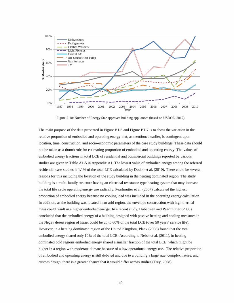
40
Figure 2-10: Number of Energy Star approved building appliances (based on USDOE, 2012)
The main purpose of the data presented in Figure B1-6 and Figure B1-7 is to show the variation in the
relative proportion of embodied and operating energy that, as mentioned earlier, is contingent upon
location, time, construction, and socio-economic parameters of the case study buildings. These data should
not be taken as a thumb rule for estimating proportion of embodied and operating energy. The values of
embodied energy fractions in total LCE of residential and commercial buildings reported by various
studies are given in Table A1-5 in Appendix A1. The lowest value of embodied energy among the referred
residential case studies is 1.1% of the total LCE calculated by Dodoo et al. (2010). There could be several
reasons for this including the location of the study building in the heating dominated region. The study
building is a multi-family structure having an electrical resistance type heating system that may increase
the total life cycle operating energy use radically. Pearlmutter et al. (2007) calculated the highest
proportion of embodied energy because no cooling load was included in the operating energy calculation.
In addition, as the building was located in an arid region, the envelope construction with high thermal
mass could result in a higher embodied energy. In a recent study, Huberman and Pearlmutter (2008)
concluded that the embodied energy of a building designed with passive heating and cooling measures in
the Negev desert region of Israel could be up to 60% of the total LCE (over 50 years’ service life).
However, in a heating dominated region of the United Kingdom, Plank (2008) found that the total
embodied energy shared only 10% of the total LCE. According to Nebel et al. (2011), in heating
dominated cold regions embodied energy shared a smaller fraction of the total LCE, which might be
higher in a region with moderate climate because of a low operational energy use. The relative proportion
of embodied and operating energy is still debated and due to a building’s large size, complex nature, and
custom design, there is a greater chance that it would differ across studies (Frey, 2008).
0%
20%
40%
60%
80%
100%
1997 1998 1999 2000 2001 2002 2003 2004 2005 2006 2007 2008 2009 2010
% M
ark
et
sha
re
Year
Dishwashers
Refrigerators
Clothes Washers
Light Fixtures
Central AC
Air-Source Heat Pump
Gas Furnaces
TV
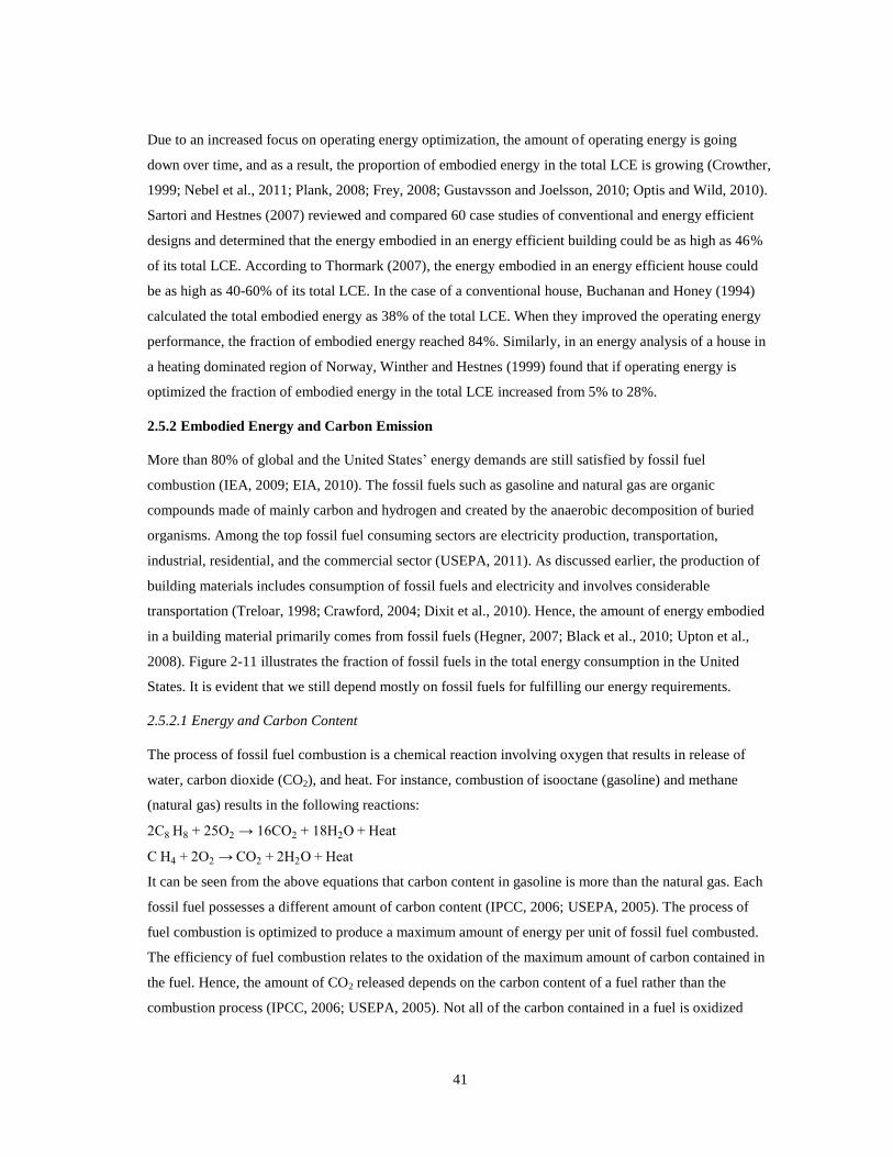
41
Due to an increased focus on operating energy optimization, the amount of operating energy is going
down over time, and as a result, the proportion of embodied energy in the total LCE is growing (Crowther,
1999; Nebel et al., 2011; Plank, 2008; Frey, 2008; Gustavsson and Joelsson, 2010; Optis and Wild, 2010).
Sartori and Hestnes (2007) reviewed and compared 60 case studies of conventional and energy efficient
designs and determined that the energy embodied in an energy efficient building could be as high as 46%
of its total LCE. According to Thormark (2007), the energy embodied in an energy efficient house could
be as high as 40-60% of its total LCE. In the case of a conventional house, Buchanan and Honey (1994)
calculated the total embodied energy as 38% of the total LCE. When they improved the operating energy
performance, the fraction of embodied energy reached 84%. Similarly, in an energy analysis of a house in
a heating dominated region of Norway, Winther and Hestnes (1999) found that if operating energy is
optimized the fraction of embodied energy in the total LCE increased from 5% to 28%.
2.5.2 Embodied Energy and Carbon Emission
More than 80% of global and the United States’ energy demands are still satisfied by fossil fuel
combustion (IEA, 2009; EIA, 2010). The fossil fuels such as gasoline and natural gas are organic
compounds made of mainly carbon and hydrogen and created by the anaerobic decomposition of buried
organisms. Among the top fossil fuel consuming sectors are electricity production, transportation,
industrial, residential, and the commercial sector (USEPA, 2011). As discussed earlier, the production of
building materials includes consumption of fossil fuels and electricity and involves considerable
transportation (Treloar, 1998; Crawford, 2004; Dixit et al., 2010). Hence, the amount of energy embodied
in a building material primarily comes from fossil fuels (Hegner, 2007; Black et al., 2010; Upton et al.,
2008). Figure 2-11 illustrates the fraction of fossil fuels in the total energy consumption in the United
States. It is evident that we still depend mostly on fossil fuels for fulfilling our energy requirements.
2.5.2.1 Energy and Carbon Content
The process of fossil fuel combustion is a chemical reaction involving oxygen that results in release of
water, carbon dioxide (CO2), and heat. For instance, combustion of isooctane (gasoline) and methane
(natural gas) results in the following reactions:
2C8 H8 25O2 16CO2 18H2O Heat
C H4 2O2 CO2 2H2O Heat
It can be seen from the above equations that carbon content in gasoline is more than the natural gas. Each
fossil fuel possesses a different amount of carbon content (IPCC, 2006; USEPA, 2005). The process of
fuel combustion is optimized to produce a maximum amount of energy per unit of fossil fuel combusted.
The efficiency of fuel combustion relates to the oxidation of the maximum amount of carbon contained in
the fuel. Hence, the amount of CO2 released depends on the carbon content of a fuel rather than the
combustion process (IPCC, 2006; USEPA, 2005). Not all of the carbon contained in a fuel is oxidized
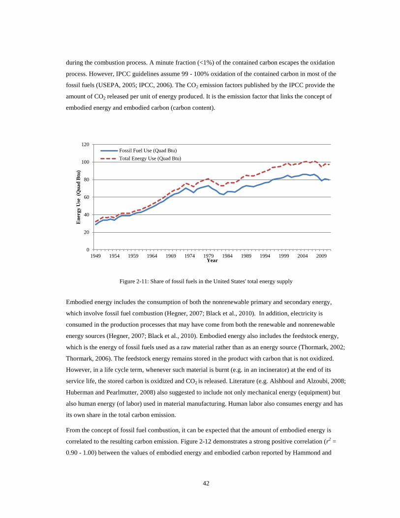
42
during the combustion process. A minute fraction (<1%) of the contained carbon escapes the oxidation
process. However, IPCC guidelines assume 99 - 100% oxidation of the contained carbon in most of the
fossil fuels (USEPA, 2005; IPCC, 2006). The CO2 emission factors published by the IPCC provide the
amount of CO2 released per unit of energy produced. It is the emission factor that links the concept of
embodied energy and embodied carbon (carbon content).
Figure 2-11: Share of fossil fuels in the United States' total energy supply
Embodied energy includes the consumption of both the nonrenewable primary and secondary energy,
which involve fossil fuel combustion (Hegner, 2007; Black et al., 2010). In addition, electricity is
consumed in the production processes that may have come from both the renewable and nonrenewable
energy sources (Hegner, 2007; Black et al., 2010). Embodied energy also includes the feedstock energy,
which is the energy of fossil fuels used as a raw material rather than as an energy source (Thormark, 2002;
Thormark, 2006). The feedstock energy remains stored in the product with carbon that is not oxidized.
However, in a life cycle term, whenever such material is burnt (e.g. in an incinerator) at the end of its
service life, the stored carbon is oxidized and CO2 is released. Literature (e.g. Alshboul and Alzoubi, 2008;
Huberman and Pearlmutter, 2008) also suggested to include not only mechanical energy (equipment) but
also human energy (of labor) used in material manufacturing. Human labor also consumes energy and has
its own share in the total carbon emission.
From the concept of fossil fuel combustion, it can be expected that the amount of embodied energy is
correlated to the resulting carbon emission. Figure 2-12 demonstrates a strong positive correlation (r2 =
0.90 - 1.00) between the values of embodied energy and embodied carbon reported by Hammond and
0
20
40
60
80
100
120
1949 1954 1959 1964 1969 1974 1979 1984 1989 1994 1999 2004 2009
En
erg
y U
se (Q
ua
d B
tu)
Year
Fossil Fuel Use (Quad Btu)
Total Energy Use (Quad Btu)
43
Jones (2008) and Gonzalez and Navarro (2006). This correlation indicates that both the embodied energy
and carbon can be used as an effective parameter for the environmental evaluation of various products
(Hegner, 2007; Acquaye, 2010).
Figure 2-12: Correlation of embodied energy and carbon
2.6 EMBODIED ENERGY CALCULATION
Two issues are very important to discuss in the context of the embodied energy calculation process. The
first issue is related to system boundary, whereas the second issue is associated with the existing embodied
energy calculation methods.
2.6.1 System Boundary Definition: Major Issues and Need for Improvement
2.6.1.1 System Boundary Definitions in the Literature
A system boundary demarcates a system of various products and processes used in the manufacturing of a
product under study. The system boundary also determines the number and type of energy and material
inputs and waste and emission outputs that are included in the embodied energy calculation (Peuportier,
2001; IFIAS, 1975). A system boundary for a product can range from raw material extraction for its
manufacturing in distant upstream to demolition and its disposal furthest downstream. Among common
system boundaries for buildings and building products are “cradle to gate,” “cradle to site,” and “cradle to
grave.” The cradle to gate system boundary includes upstream processes such as raw material extraction
R² = 0.89
R² = 1.00
0
1
2
3
4
5
6
7
8
9
0 20 40 60 80 100 120 140 160 180 200
Em
bo
die
d C
O2
(K
gC
O2
/kg
)
Embodied Energy (MJ/kg)
Hammond & Jones, 2008
Gonzalez & Navarro, 2006
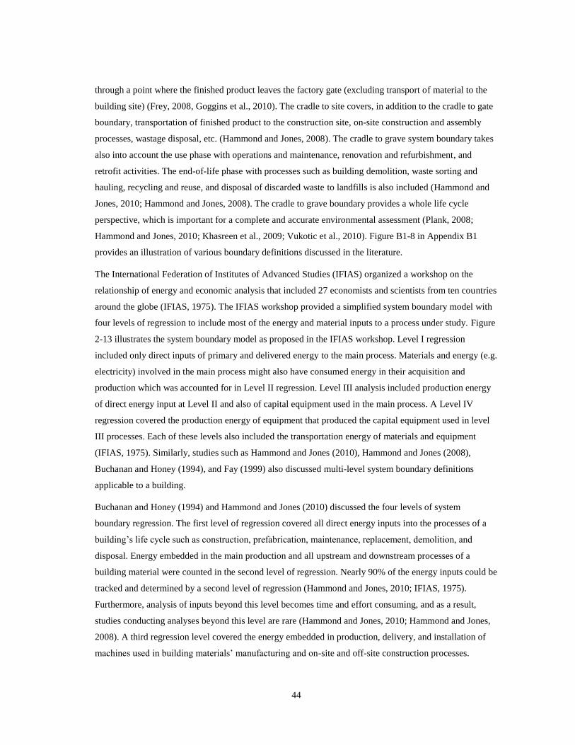
44
through a point where the finished product leaves the factory gate (excluding transport of material to the
building site) (Frey, 2008, Goggins et al., 2010). The cradle to site covers, in addition to the cradle to gate
boundary, transportation of finished product to the construction site, on-site construction and assembly
processes, wastage disposal, etc. (Hammond and Jones, 2008). The cradle to grave system boundary takes
also into account the use phase with operations and maintenance, renovation and refurbishment, and
retrofit activities. The end-of-life phase with processes such as building demolition, waste sorting and
hauling, recycling and reuse, and disposal of discarded waste to landfills is also included (Hammond and
Jones, 2010; Hammond and Jones, 2008). The cradle to grave boundary provides a whole life cycle
perspective, which is important for a complete and accurate environmental assessment (Plank, 2008;
Hammond and Jones, 2010; Khasreen et al., 2009; Vukotic et al., 2010). Figure B1-8 in Appendix B1
provides an illustration of various boundary definitions discussed in the literature.
The International Federation of Institutes of Advanced Studies (IFIAS) organized a workshop on the
relationship of energy and economic analysis that included 27 economists and scientists from ten countries
around the globe (IFIAS, 1975). The IFIAS workshop provided a simplified system boundary model with
four levels of regression to include most of the energy and material inputs to a process under study. Figure
2-13 illustrates the system boundary model as proposed in the IFIAS workshop. Level I regression
included only direct inputs of primary and delivered energy to the main process. Materials and energy (e.g.
electricity) involved in the main process might also have consumed energy in their acquisition and
production which was accounted for in Level II regression. Level III analysis included production energy
of direct energy input at Level II and also of capital equipment used in the main process. A Level IV
regression covered the production energy of equipment that produced the capital equipment used in level
III processes. Each of these levels also included the transportation energy of materials and equipment
(IFIAS, 1975). Similarly, studies such as Hammond and Jones (2010), Hammond and Jones (2008),
Buchanan and Honey (1994), and Fay (1999) also discussed multi-level system boundary definitions
applicable to a building.
Buchanan and Honey (1994) and Hammond and Jones (2010) discussed the four levels of system
boundary regression. The first level of regression covered all direct energy inputs into the processes of a
building’s life cycle such as construction, prefabrication, maintenance, replacement, demolition, and
disposal. Energy embedded in the main production and all upstream and downstream processes of a
building material were counted in the second level of regression. Nearly 90% of the energy inputs could be
tracked and determined by a second level of regression (Hammond and Jones, 2010; IFIAS, 1975).
Furthermore, analysis of inputs beyond this level becomes time and effort consuming, and as a result,
studies conducting analyses beyond this level are rare (Hammond and Jones, 2010; Hammond and Jones,
2008). A third regression level covered the energy embedded in production, delivery, and installation of
machines used in building materials’ manufacturing and on-site and off-site construction processes.
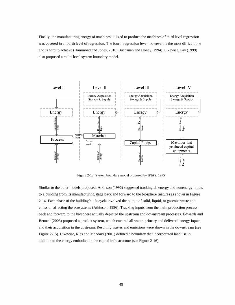
45
Finally, the manufacturing energy of machines utilized to produce the machines of third level regression
was covered in a fourth level of regression. The fourth regression level, however, is the most difficult one
and is hard to achieve (Hammond and Jones, 2010; Buchanan and Honey, 1994). Likewise, Fay (1999)
also proposed a multi-level system boundary model.
Figure 2-13: System boundary model proposed by IFIAS, 1975
Similar to the other models proposed, Atkinson (1996) suggested tracking all energy and nonenergy inputs
to a building from its manufacturing stage back and forward to the biosphere (nature) as shown in Figure
2-14. Each phase of the building’s life cycle involved the output of solid, liquid, or gaseous waste and
emission affecting the ecosystems (Atkinson, 1996). Tracking inputs from the main production process
back and forward to the biosphere actually depicted the upstream and downstream processes. Edwards and
Bennett (2003) proposed a product system, which covered all water, primary and delivered energy inputs,
and their acquisition in the upstream. Resulting wastes and emissions were shown in the downstream (see
Figure 2-15). Likewise, Ries and Mahdavi (2001) defined a boundary that incorporated land use in
addition to the energy embodied in the capital infrastructure (see Figure 2-16).
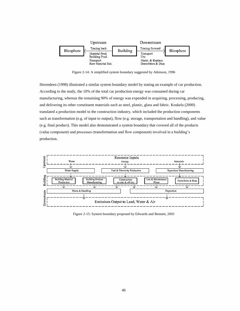
46
Figure 2-14: A simplified system boundary suggested by Atkinson, 1996
Herendeen (1998) illustrated a similar system boundary model by stating an example of car production.
According to the study, the 10% of the total car production energy was consumed during car
manufacturing, whereas the remaining 90% of energy was expended in acquiring, processing, producing,
and delivering its other constituent materials such as steel, plastic, glass and fabric. Koskela (2000)
translated a production model to the construction industry, which included the production components
such as transformation (e.g. of input to output), flow (e.g. storage, transportation and handling), and value
(e.g. final product). This model also demonstrated a system boundary that covered all of the products
(value component) and processes (transformation and flow component) involved in a building’s
production.
Figure 2-15: System boundary proposed by Edwards and Bennett, 2003
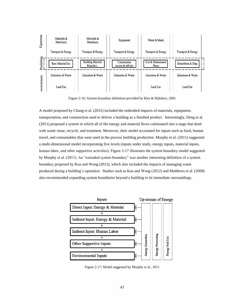
47
Figure 2-16: System boundary definition provided by Ries & Mahdavi, 2001
A model proposed by Chang et al. (2012) included the embodied impacts of materials, equipment,
transportation, and construction used to deliver a building as a finished product. Interestingly, Deng et al.
(2011) proposed a system in which all of the energy and material flows culminated into a stage that dealt
with waste reuse, recycle, and treatment. Moreover, their model accounted for inputs such as food, human
travel, and consumables that were used in the process building production. Murphy et al. (2011) suggested
a multi-dimensional model incorporating five levels (inputs under study, energy inputs, material inputs,
human labor, and other supportive activities). Figure 2-17 illustrates the system boundary model suggested
by Murphy et al. (2011). An “extended system boundary” was another interesting definition of a system
boundary proposed by Kua and Wong (2012), which also included the impacts of managing waste
produced during a building’s operation. Studies such as Kua and Wong (2012) and Matthews et al. (2008)
also recommended expanding system boundaries beyond a building to its immediate surroundings.
Figure 2-17: Model suggested by Murphy et al., 2011
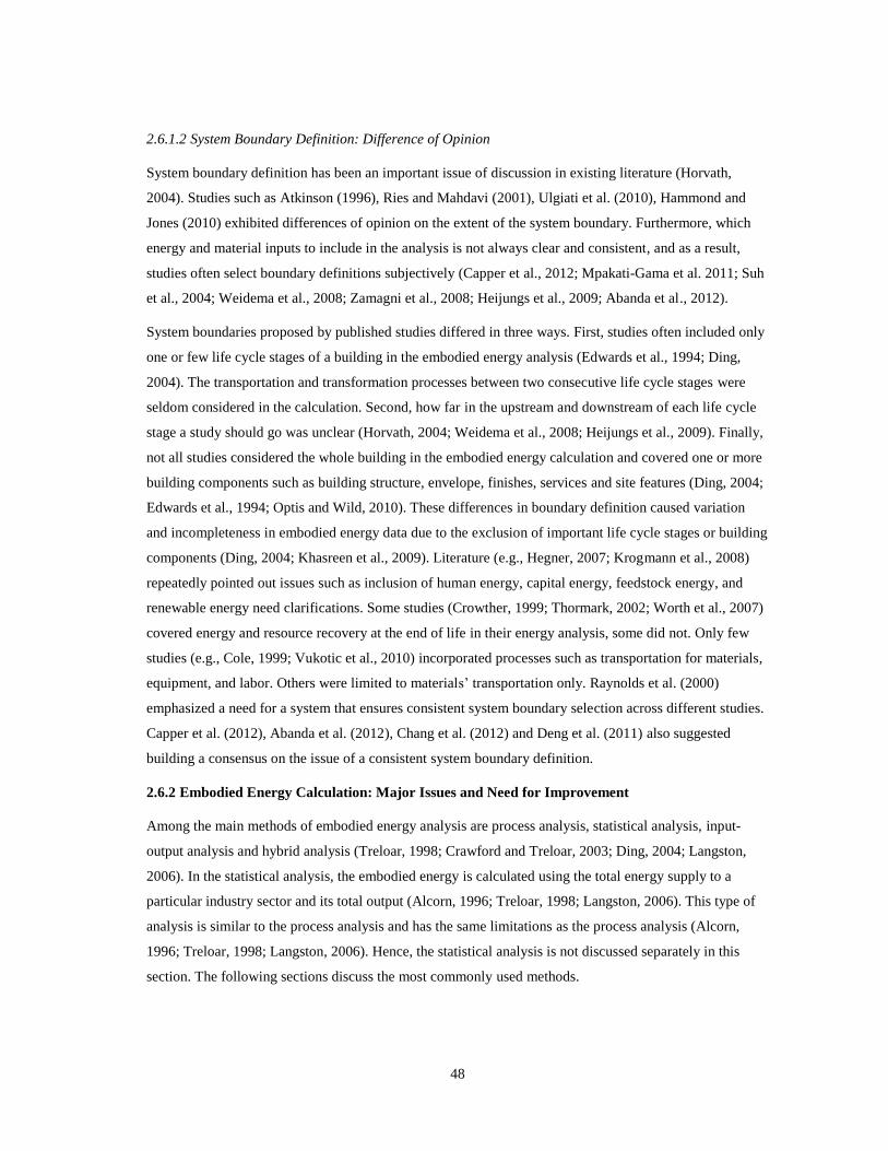
48
2.6.1.2 System Boundary Definition: Difference of Opinion
System boundary definition has been an important issue of discussion in existing literature (Horvath,
2004). Studies such as Atkinson (1996), Ries and Mahdavi (2001), Ulgiati et al. (2010), Hammond and
Jones (2010) exhibited differences of opinion on the extent of the system boundary. Furthermore, which
energy and material inputs to include in the analysis is not always clear and consistent, and as a result,
studies often select boundary definitions subjectively (Capper et al., 2012; Mpakati-Gama et al. 2011; Suh
et al., 2004; Weidema et al., 2008; Zamagni et al., 2008; Heijungs et al., 2009; Abanda et al., 2012).
System boundaries proposed by published studies differed in three ways. First, studies often included only
one or few life cycle stages of a building in the embodied energy analysis (Edwards et al., 1994; Ding,
2004). The transportation and transformation processes between two consecutive life cycle stages were
seldom considered in the calculation. Second, how far in the upstream and downstream of each life cycle
stage a study should go was unclear (Horvath, 2004; Weidema et al., 2008; Heijungs et al., 2009). Finally,
not all studies considered the whole building in the embodied energy calculation and covered one or more
building components such as building structure, envelope, finishes, services and site features (Ding, 2004;
Edwards et al., 1994; Optis and Wild, 2010). These differences in boundary definition caused variation
and incompleteness in embodied energy data due to the exclusion of important life cycle stages or building
components (Ding, 2004; Khasreen et al., 2009). Literature (e.g., Hegner, 2007; Krogmann et al., 2008)
repeatedly pointed out issues such as inclusion of human energy, capital energy, feedstock energy, and
renewable energy need clarifications. Some studies (Crowther, 1999; Thormark, 2002; Worth et al., 2007)
covered energy and resource recovery at the end of life in their energy analysis, some did not. Only few
studies (e.g., Cole, 1999; Vukotic et al., 2010) incorporated processes such as transportation for materials,
equipment, and labor. Others were limited to materials’ transportation only. Raynolds et al. (2000)
emphasized a need for a system that ensures consistent system boundary selection across different studies.
Capper et al. (2012), Abanda et al. (2012), Chang et al. (2012) and Deng et al. (2011) also suggested
building a consensus on the issue of a consistent system boundary definition.
2.6.2 Embodied Energy Calculation: Major Issues and Need for Improvement
Among the main methods of embodied energy analysis are process analysis, statistical analysis, input-
output analysis and hybrid analysis (Treloar, 1998; Crawford and Treloar, 2003; Ding, 2004; Langston,
2006). In the statistical analysis, the embodied energy is calculated using the total energy supply to a
particular industry sector and its total output (Alcorn, 1996; Treloar, 1998; Langston, 2006). This type of
analysis is similar to the process analysis and has the same limitations as the process analysis (Alcorn,
1996; Treloar, 1998; Langston, 2006). Hence, the statistical analysis is not discussed separately in this
section. The following sections discuss the most commonly used methods.

49
2.6.2.1 Process-based Embodied Energy Analysis
Process-based analysis is one of the most widely used methods of embodied energy (EE) analysis, as it
delivers more accurate (Ding, 2004) and reliable results (Alcorn and Baird, 1996; Pullen, 2000b; Crawford
and Treloar, 2003). The process commences with the building material as a final product and works
backward in the upstream of the main process, taking into account most of the direct and indirect energy
inputs embodied in each constituent material (Treloar, 1998; Alcorn and Baird, 1996). As discussed in
Section 1.3, the embodied energy of a product is the sum of directly and indirectly consumed energy in its
production. Hence, for a complete calculation both the direct and indirect energy data are required
(Treloar, 1998; Crawford, 2004).
However, in the case of a process-based energy analysis, it is difficult to track most indirect energy inputs.
For instance, take a generic example of using concrete and steel in a structure. Figure 2-18 illustrates the
generic example. The construction of the structure shown in Figure 2-18 involves direct (Edi) and indirect
energy use (spread over Stage 1 through n as marked in Figure 2-18). The direct energy requirements
represent the construction energy consumed in operating construction vehicles, cranes, earthmovers, and
power tools and in temporary space conditioning at the construction site. The indirect energy requirements
account for the energy embedded in materials (e.g., concrete, rebar as shown in Figure 2-18) and services
(architectural and engineering services as shown in Figure 2-18) used in building construction (Treloar,
1998; Crawford, 2004; Acquaye, 2010). In the case of a process-based analysis, energy embodied in
concrete can be calculated if the embodied energy of Portland cement is known. Similarly, the embodied
energy of Portland cement can be determined if the data about energy contents of clinker are available. By
going in the upstream of, for instance concrete, one can track most of the indirect energy inputs. However,
after a certain point in the upstream, the tracking of energy inputs is truncated due to the unavailability of
data (Treloar, 1998; Crawford, 2004; Acquaye, 2010) or enormous efforts required to identify and
quantify each material and energy input to the complex upstream processes (Alcorn and Baird, 1996;
Treloar et al., 2001b; Ding, 2004; Crawford and Treloar, 2005). This causes a truncation error, which is
actually an issue of incompleteness. Technically, this is called a system boundary truncation. Even
downstream truncation of system boundary occurs in a process-based analysis (Acquaye, 2010). For
instance, in the case of steel mills, downstream processes of fabricating rebar are truncated because the
weight of rebar is multiplied by the embodied energy coefficient of steel to calculate the embodied energy
of rebar. This excludes the direct energy consumed by manufacturing units fabricating rebar and other
structural shapes. Other services such as banking, insurance, architectural and engineering consultancy,
construction management, and commissioning are mostly excluded from the calculation causing a
complete truncation of services.
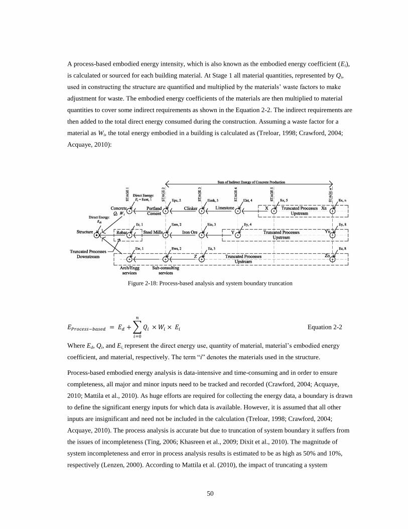
50
A process-based embodied energy intensity, which is also known as the embodied energy coefficient (Ei),
is calculated or sourced for each building material. At Stage 1 all material quantities, represented by Qi,
used in constructing the structure are quantified and multiplied by the materials’ waste factors to make
adjustment for waste. The embodied energy coefficients of the materials are then multiplied to material
quantities to cover some indirect requirements as shown in the Equation 2-2. The indirect requirements are
then added to the total direct energy consumed during the construction. Assuming a waste factor for a
material as Wi, the total energy embodied in a building is calculated as (Treloar, 1998; Crawford, 2004;
Acquaye, 2010):
Figure 2-18: Process-based analysis and system boundary truncation
∑
Equation 2-2
Where Ed, Qi, and Ei, represent the direct energy use, quantity of material, material’s embodied energy
coefficient, and material, respectively. The term “i” denotes the materials used in the structure.
Process-based embodied energy analysis is data-intensive and time-consuming and in order to ensure
completeness, all major and minor inputs need to be tracked and recorded (Crawford, 2004; Acquaye,
2010; Mattila et al., 2010). As huge efforts are required for collecting the energy data, a boundary is drawn
to define the significant energy inputs for which data is available. However, it is assumed that all other
inputs are insignificant and need not be included in the calculation (Treloar, 1998; Crawford, 2004;
Acquaye, 2010). The process analysis is accurate but due to truncation of system boundary it suffers from
the issues of incompleteness (Ting, 2006; Khasreen et al., 2009; Dixit et al., 2010). The magnitude of
system incompleteness and error in process analysis results is estimated to be as high as 50% and 10%,
respectively (Lenzen, 2000). According to Mattila et al. (2010), the impact of truncating a system

51
boundary could be up to 20% or more, particularly in sectors dominated by capital investments. Pullen
(2000b) stated that the process analysis fails to capture not only some of the downstream processes but
also the capital energy inputs (e.g. plants and equipment) required for building material production. If a
system boundary model is developed based on the IFIAS recommendations (see Figure 2-13), it is more
likely that the calculation remains incomplete if a process-based analysis is used. Even inventories based
on a detailed and extensive process analysis failed to attain a reasonable completeness (Treloar et al.,
2001b; Crawford, 2004; Crawford and Treloar, 2005). Crawford (2004) also discussed a sideways
truncation that occurred because of inputs to the main process extending sideways.
According to literature (e.g., Treloar, 1998; Crawford, 2004; Acquaye, 2010), most process-based studies
could go up to Stage 2 if extensive data is available. According to Baird et al. (1994), Stage 1, which
mainly covered direct energy inputs, represented less than 50% of the total energy requirements. At Stage
2, nearly 40% energy use was covered, whereas beyond Stage 2, only 10% of energy inputs were left. This
meant that if an analysis was conducted up to Stage 2 completely, nearly 90% of the gross energy
requirements of a building could have been covered.
2.6.2.2 Input-output-based Embodied Energy Analysis
An input-output-based analysis is conducted on the basis of economic data and it utilizes the monetary
flows among different industry sectors to determine energy embodied in a particular product (Treloar,
1998; Crawford, 2004; Acquaye, 2010). These economic data are published periodically by the
governments in the form of input-output tables. An economic input-output table presents monetary flows
among various industries of a given economy. An economy on the globe can be divided into numerous
sectors that produce a variety of products. These sectors represent one industry or a group of industries
that produce a similar product (e.g. steel products). Each sector that manufactures a product also
consumes goods and services produced by other sectors (Carter et al., 1981; Miller and Blair, 2009). This
creates an interindustry flow of inputs and outputs where the sum of the inputs of a sector equals the sum
of its outputs to other sectors. An input-output table demonstrates these interindustry transactions as well
as consumption and purchases made by the final consumers and government. The input-output table
contains sectors that produce goods and services and also consume goods and services produced by other
sectors.
An economic input-output table is always in equilibrium meaning that the inputs and the outputs of the
industry sectors are balanced (Miernyk, 1965; Carter et al., 1981; Miller and Blair, 2009). This means that
if an industry sector increases its output by one dollar, then by the input-output theory, it will require
inputs worth one dollar more from its supplying sector. The demand from its supplying sector is known as
the direct requirement. Each supplying sector also needs to buy more to meet the demand of this increased
output. Hence, the impact of increasing output by one dollar can be felt throughout the economy. This
52
impact represents the indirect requirements. The sum of direct and indirect requirements is termed the total
requirements (Miernyk, 1965; Miller and Blair, 2009). In an input-output-based energy analysis, the total
impact of a one dollar increase in the output of an industry sector on the energy providing sectors is
calculated from the total requirement coefficients. After determining the monetary inputs required from
the energy sectors per dollar output, energy tariff can be used to derive the total energy consumption in
energy units. The direct and total requirement coefficients are converted to direct and total energy
requirement coefficients using fixed or variable energy prices. The input-output tables have been used to
transcribe economic flows into energy flows by applying average energy tariffs (Fay and Treloar, 1998;
Crawford and Treloar, 2003; Ding, 2004). Thus, in an input-output analysis, the cost of a product and its
energy intensity (in MJ/$) are multiplied to compute its embodied energy (Crawford and Treloar, 2005).
The input-output-based analysis accounts for most direct and indirect energy inputs used in the process of
building material production and thus is considered complete (Fay and Treloar, 1998). Figure 2-19
illustrates the same generic example in an input-output context. As the total requirement coefficients
represent the sum of direct and indirect requirements, this method is assumed to be comprehensive and
complete as it embraces nearly the entire system boundary as shown in Figure 2-19. If Ti and Di represent
the total and direct requirement coefficient in $ input/$ output of an industry sector “i”, the total and direct
energy requirements are given by:
Figure 2-19: Input-output analysis and system boundary coverage

53
Where Fp is the energy price in MJ/$. The calculated energy coefficients provide total and direct energy
use in MJ/$ industry output. The total energy requirements can be calculated by multiplying the TEi and
total industry output Ot ($).
Equation 2-3
Although this method is considered complete, it also suffers from inherent problems such as errors and
uncertainties of economic data (e.g. energy tariff and product cost) and aggregation of industry sectors.
The issue of aggregation makes the end results less specific to the product under study. For example, a
residential construction sector may represent all residential buildings including low-rise, high-rise,
custom-designed, and mass housing. As per the input-output theory, all of them would have the same
energy intensity as the residential sector, which may not be true. Although the results of an input-output-
based analysis are less study-specific than the process-based analysis, it is still considered straightforward,
accessible, and representative (Langston, 2006; Pullen, 1996). Among the major limitations of input-
output-based methods include:
Age of Data: The input-output tables are not published in a timely manner due to extensive efforts
involved in collecting, analyzing, and balancing the economic data. Usually, economic input-output tables
are five or more years old making its data nonrepresentative in time (Crawford, 2004; Langston, 2006;
Miller and Blair, 2009). For instance, the United States’ detailed input-output accounts are published every
seven years. The latest benchmark data that are available are from 2002 (USBEA, 2008). Two types of
anomalies could arise due to the use of old data. First, the structure of the domestic and foreign monetary
transaction might have changed over time. Second, the composition of labor and machine in the
production function might have altered as a result of improved technology.
National Average and Fixed Energy Tariff: To convert monetary transactions into energy terms,
national average prices are used that may not represent the actual energy prices paid by the industry
sectors. The fuel mix for electricity production and input composition for material production also differ
with geographic location (Crawford, 2004) within the same country. Some industries pay real-time
electricity prices, whereas some end up paying peak rate charges. Also, energy buyers usually negotiate
while purchasing energy in bulk. Using a national average price to convert monetary flows into energy
flows may not be representative (Treloar, 1998; Crawford, 2004; Miller and Blair, 2009; Acquaye, 2010).
Instead of using variable prices, fixed energy tariffs are used to derive a national average by converting
monetary data to energy data. In reality, sectors may be paying different prices for different energy types
such as oil, natural gas, and coal (Langston, 2006; Crawford et al., 2002; Carter et al., 1981; Crawford,
2004).
Proportionality Assumptions: The cost of the product of each sector in an input-output table is directly
proportional to the amount of goods and services consumed by that sector. For instance, if 50 kilograms of

54
steel is needed to manufacture a refrigerator then 100 kilograms of steel would be needed to produce two
refrigerators of the same cost (Langston, 2006; Crawford, 2004; Crawford et al., 2002). In energy terms,
for instance, if 1 MBtu is consumed to produce 1 lb of steel then to produce 5 lbs. of steel, 5 MBtu of
energy would be required. This may not hold true, as manufacturing industries use different production
technologies and their energy and material input could be quite different from one another (Acquaye,
2010).
Homogeneity Assumptions: Input-output tables are built assuming that the same mix of inputs (product
and services) is required by each product manufactured by an industry sector. This means that all products
covered under the aluminum sector are manufactured using the same mix of inputs (e.g. bauxite,
electricity, accounting services, etc.), which may not be true, especially for a sector that is highly
aggregated (Langston, 2006; Crawford, 2004; Treloar, 1998; Crawford et al., 2002). Aluminum cans, for
instance, would require a different mix of inputs than a cooking utensil of the same weight. According to
the homogeneity assumption, the aluminum cans could be substituted for the cooking utensil, which may
be accurate in monetary terms but may not be in physical terms (Treloar, 1998; Crawford, 2004)
Aggregation Problem: Input-output tables are composed of sectors that are highly aggregated. These
sectors represent more than one product and each product may have a different energy intensity and price
(Langston, 2006; Crawford, 2004; Treloar, 1997). For instance, an industry sector manufacturing plastic
goods would represent, in energy terms, all plastic products related to construction, medical supply,
packaging, machinery, electronic items, etc. Given this assumption, each of these plastic products would
share the same energy intensity as the industry sector as a whole. In reality, this assumption is not true, as
each of the listed products has a different energy intensity (Crawford, 2004; Acquaye, 2010).
Double Counting: According to Treloar (1998) and Langston (2006), energy may be double counted
while using input-output data for energy providing sectors. For instance, if 1 GJ of electricity is produced
using 2 GJ of oil then the energy embodied in electricity would be 3 GJ as per input-output theory
(Treloar, 1998). Another example of double counting is the energy intensity of an energy providing sector.
For example, in the United States, the dry natural gas is distributed by the Natural Gas Distribution sector.
If an industry sector purchased natural gas from the Natural Gas Distribution sector, the purchased natural
gas would be double counted as an indirect impact because the Natural Gas Distribution sector also
bought natural gas from the Oil and Gas Extraction sector.
Exclusion of Inputs: Inputs such as capital goods are not purchased or replaced frequently. Such goods
may not show up in the input-output tables for a given year (Treloar, 1998; Crawford, 2004; Langston,
2006). In addition, since household expenditure is treated as a final demand component, the use of human
energy by manufacturing sectors remains excluded from the input-output calculations.
55
The assumptions and various issues with economic input-output data make results of an input-output-
based analysis erroneous and unreliable (Fay and Treloar, 1998; Crawford and Treloar, 2003; Ting, 2006;
Pearlmutter et al., 2007; Khasreen et al., 2009). The resulting error in the measurement could be up to
50% (Treloar et al., 2001a).
2.6.2.3 Hybrid Analysis
The process-based analysis is specific to the study but lacks completeness. The input-output-based
analysis is complete but lacks specificity (Dixit et al., 2012a). A hybrid analysis is devised by unifying the
benefits of the two methods to eliminate the fundamental errors and limitations of both the process and
input-output-based analyses (Mattila et al., 2010; Acquaye, 2010; Dixit et al., 2012a). However, the results
of a hybrid method also need to be compared and validated (Crawford and Treloar, 2003).
The hybrid method starts with process analysis of readily available energy input data of the final
production stage and likely one stage more in the upstream. In later upstream stages when it becomes
difficult to achieve reliable and consistent information about complex upstream processes, the process
analysis is substituted by the input-output-based analysis (Alcorn and Baird, 1996; Lenzen, 2000). There
are many ways in which the two methods can be combined. The ultimate aim is to improve specificity,
accuracy, and completeness of the method. Literature (e.g., Crawford, 2004; Treloar, 1998; Dixit et al.,
2010; Acquaye, 2010) categorized hybrid methods as:
Process-based Hybrid Analysis: This method applies input-output-based analysis to complex parts of
upstream processes of material production and thus, obviates the incompleteness inherent in process
analysis. In this method, the material quantities used in a building are quantified using the process data
(e.g. bill of quantities). According to Treloar (1998), the calculated material quantities are then multiplied
by input-output-based energy intensities of each material. The input-output -based energy intensities that
are in energy unit per $ (e.g. MJ/$) are converted into physical quantities using the price of the material
(Treloar, 1998). Treloar (1998) also warned that if material prices are underestimated or overestimated, the
embodied energy values would be grossly affected. However, using this method for a complex product,
which is made of more than one material, could pose problems, as the manufacturing energy of the
complex product is mostly excluded. Figure 2-20 illustrates this issue by an example of open web joists.
For quantifying the energy embodied in an open web joist, the quantity of steel (Qi) is derived and
multiplied by the input-output -based embodied energy coefficient of steel. However, in the process, other
upstream inputs (as marked in the dashed box) are left behind. Also, as only steel quantities are used, the
direct energy (Edi as shown in Figure 2-20) consumed in fabricating open web joists is also excluded from
the calculation. According to Treloar (1998), incompleteness due to this issue could be 0-100%.
Input-output-Based Hybrid Analysis: This method involves substitution of input-output data by process
data in an input-output model in order to improve reliability of the energy calculation (Treloar, 1998;
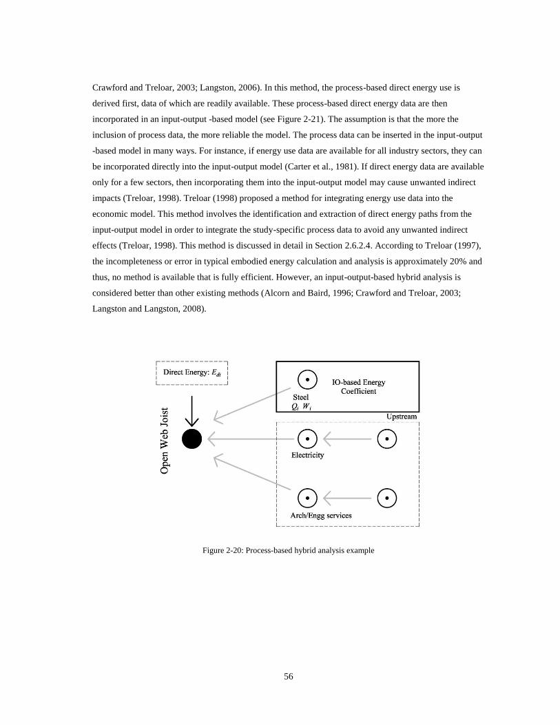
56
Crawford and Treloar, 2003; Langston, 2006). In this method, the process-based direct energy use is
derived first, data of which are readily available. These process-based direct energy data are then
incorporated in an input-output -based model (see Figure 2-21). The assumption is that the more the
inclusion of process data, the more reliable the model. The process data can be inserted in the input-output
-based model in many ways. For instance, if energy use data are available for all industry sectors, they can
be incorporated directly into the input-output model (Carter et al., 1981). If direct energy data are available
only for a few sectors, then incorporating them into the input-output model may cause unwanted indirect
impacts (Treloar, 1998). Treloar (1998) proposed a method for integrating energy use data into the
economic model. This method involves the identification and extraction of direct energy paths from the
input-output model in order to integrate the study-specific process data to avoid any unwanted indirect
effects (Treloar, 1998). This method is discussed in detail in Section 2.6.2.4. According to Treloar (1997),
the incompleteness or error in typical embodied energy calculation and analysis is approximately 20% and
thus, no method is available that is fully efficient. However, an input-output-based hybrid analysis is
considered better than other existing methods (Alcorn and Baird, 1996; Crawford and Treloar, 2003;
Langston and Langston, 2008).
Figure 2-20: Process-based hybrid analysis example
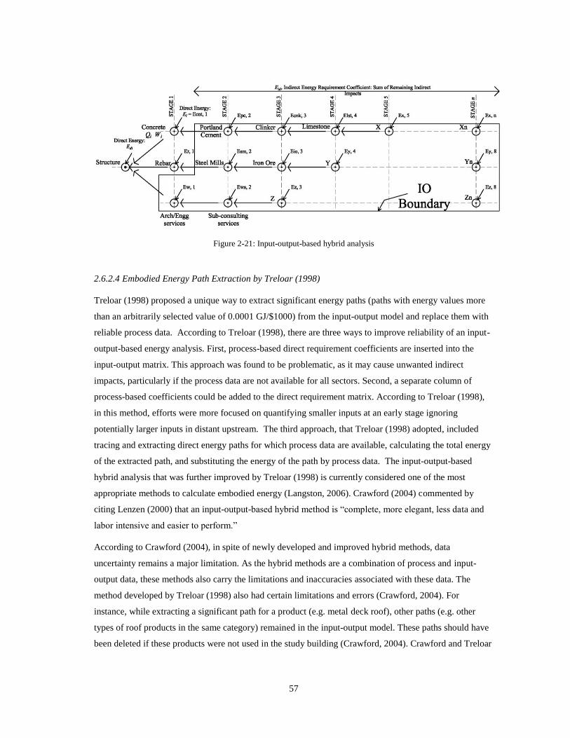
57
Figure 2-21: Input-output-based hybrid analysis
2.6.2.4 Embodied Energy Path Extraction by Treloar (1998)
Treloar (1998) proposed a unique way to extract significant energy paths (paths with energy values more
than an arbitrarily selected value of 0.0001 GJ/$1000) from the input-output model and replace them with
reliable process data. According to Treloar (1998), there are three ways to improve reliability of an input-
output-based energy analysis. First, process-based direct requirement coefficients are inserted into the
input-output matrix. This approach was found to be problematic, as it may cause unwanted indirect
impacts, particularly if the process data are not available for all sectors. Second, a separate column of
process-based coefficients could be added to the direct requirement matrix. According to Treloar (1998),
in this method, efforts were more focused on quantifying smaller inputs at an early stage ignoring
potentially larger inputs in distant upstream. The third approach, that Treloar (1998) adopted, included
tracing and extracting direct energy paths for which process data are available, calculating the total energy
of the extracted path, and substituting the energy of the path by process data. The input-output-based
hybrid analysis that was further improved by Treloar (1998) is currently considered one of the most
appropriate methods to calculate embodied energy (Langston, 2006). Crawford (2004) commented by
citing Lenzen (2000) that an input-output-based hybrid method is “complete, more elegant, less data and
labor intensive and easier to perform.”
According to Crawford (2004), in spite of newly developed and improved hybrid methods, data
uncertainty remains a major limitation. As the hybrid methods are a combination of process and input-
output data, these methods also carry the limitations and inaccuracies associated with these data. The
method developed by Treloar (1998) also had certain limitations and errors (Crawford, 2004). For
instance, while extracting a significant path for a product (e.g. metal deck roof), other paths (e.g. other
types of roof products in the same category) remained in the input-output model. These paths should have
been deleted if these products were not used in the study building (Crawford, 2004). Crawford and Treloar
58
(2003) demonstrated an approach to carefully extract all paths that were used or not used in the study
building and then insert relevant process data. Treloar et al. (2000) also warned that even if significant
energy paths were extracted and replaced with reliable process data, unimportant energy paths remained in
the model that still acted as a “black box.” The input-output-based hybrid method proposed by Treloar
(1998) requires process data, which may not be representative, accurate, or complete. For instance, Treloar
(2001c) utilized the same method to calculate energy embodied in office buildings and obtained process
data from a variety of sources. Although care was taken not to select process data that are more than five
years old, the sourced process data may not be complete or representative. In addition, if process energy
data are available for most of the industry sectors, it would be much easier to modify a column of an input-
output model without unwanted indirect effects as shown by Carter et al. (1981). According to Treloar
(1998), energy use data are only available for 25 industry sectors out of the total 113 sectors of the
Australian economy. Hendrickson et al. (1997) concluded that life cycle assessment at a more refined level
may not be meaningful given the uncertainty of life cycle data. Crawford (2004) (by citing Crawford et al.,
2003) believed that efforts to improve reliability and completeness are “still worthwhile.”
2.6.2.5 Improvements in Treloar’s Method by Crawford (2004)
Some of the problems identified in the embodied energy path extraction approach proposed by Treloar
(1998) were resolved by Crawford (2004). Crawford’s approach was useful in calculating the embodied
energy of particularly complex products that are made of multiple basic materials. For instance, in
quantifying the energy embodied in concrete that is composed of cement, aggregates, steel, and water, this
method ensured the inclusion of all direct and indirect inputs associated with a ready-mix plant in addition
to the collective embodied energy of its constituent materials. The approach proposed by Crawford (2004)
involved three main steps:
Step I: Calculation of the process-based hybrid energy intensity of each constituent material (e.g. in the
case of the concrete example, cement, aggregates, steel, and water) by adding the process-based energy
intensity and extracting the total energy of the total energy path representing each constituent material
from its input-output sector:
( ) Equation 2-4
Where:
i Representing a constituent material (e.g. cement)
Process-based hybrid energy intensity of the constituent material
Process-based energy intensity of the constituent material
Total energy intensity of input-output sector manufacturing the constituent material
Total energy of the total energy path representing the constituent material
Price of the constituent material
59
Step II: The process-based hybrid embodied energy of a complex product “p” is calculated as:
Equation 2-5
Where:
p Representing a complex product (e.g. concrete)
Process-based hybrid energy intensity of the product
Quantity of the constituent material
Waste factor of the constituent material
Process-based hybrid energy intensity of the constituent material
Direct energy intensity of input-output sector manufacturing the product
Price of the product
Step III: The IO-based hybrid embodied energy of a complex product is calculated as:
( ) Equation 2-6
Where:
p Representing a complex product (e.g. concrete)
IO-based hybrid energy intensity of the product
Quantity of the constituent material
Waste factor of the constituent material
Process-based energy intensity of the constituent material
Total energy intensity of IO sector manufacturing the product
Total energy of the total energy path representing the product
Price of the product
2.6.2.6 Issue with the Proposed Hybrid Methods
The input-output-based hybrid methods proposed by Treloar (1998) and Crawford (2004) were very
useful, especially when determining the embodied energy of a complex product in an economy where
process energy data are available for some of the industry sectors. However, there was an assumption that
the process-based energy intensities were calculated in a complete and accurate manner. For instance,
inputs such as human energy might not be included in the available process data. It is still not clear how to
incorporate human and capital inputs in the calculation. In addition, while calculating the process-based
hybrid energy intensity of a constituent material (Step I in the Crawford’s method), when the energy of the
total energy path (Ti) was extracted, both the direct and indirect energy were excluded. However, the
energy replaced by the process-based value (Ep, i) might not include the indirect energy of the constituent
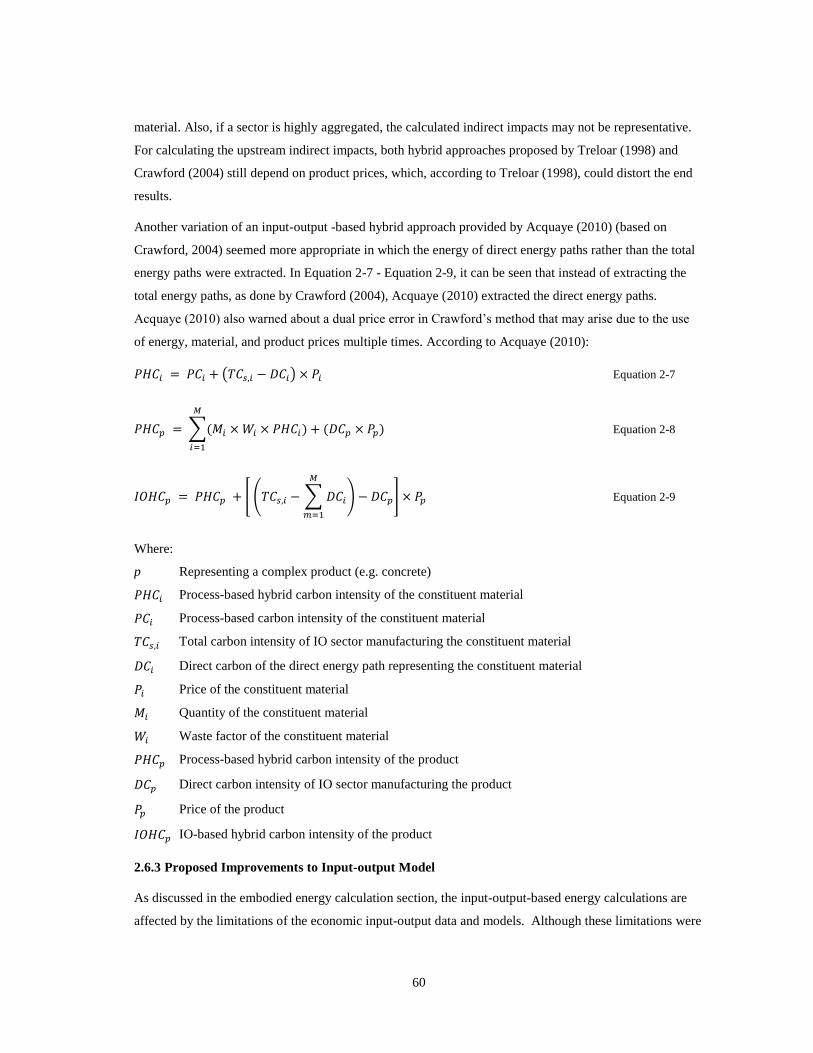
60
material. Also, if a sector is highly aggregated, the calculated indirect impacts may not be representative.
For calculating the upstream indirect impacts, both hybrid approaches proposed by Treloar (1998) and
Crawford (2004) still depend on product prices, which, according to Treloar (1998), could distort the end
results.
Another variation of an input-output -based hybrid approach provided by Acquaye (2010) (based on
Crawford, 2004) seemed more appropriate in which the energy of direct energy paths rather than the total
energy paths were extracted. In Equation 2-7 - Equation 2-9, it can be seen that instead of extracting the
total energy paths, as done by Crawford (2004), Acquaye (2010) extracted the direct energy paths.
Acquaye (2010) also warned about a dual price error in Crawford’s method that may arise due to the use
of energy, material, and product prices multiple times. According to Acquaye (2010):
( ) Equation 2-7
∑
Equation 2-8
[ ( ∑
) ] Equation 2-9
Where:
p Representing a complex product (e.g. concrete)
Process-based hybrid carbon intensity of the constituent material
Process-based carbon intensity of the constituent material
Total carbon intensity of IO sector manufacturing the constituent material
Direct carbon of the direct energy path representing the constituent material
Price of the constituent material
Quantity of the constituent material
Waste factor of the constituent material
Process-based hybrid carbon intensity of the product
Direct carbon intensity of IO sector manufacturing the product
Price of the product
IO-based hybrid carbon intensity of the product
2.6.3 Proposed Improvements to Input-output Model
As discussed in the embodied energy calculation section, the input-output-based energy calculations are
affected by the limitations of the economic input-output data and models. Although these limitations were
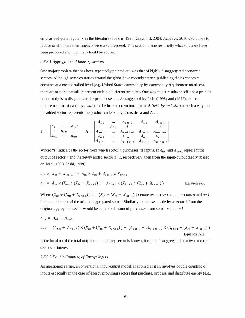
61
emphasized quite regularly in the literature (Treloar, 1998; Crawford, 2004; Acquaye, 2010), solutions to
reduce or eliminate their impacts were also proposed. This section discusses briefly what solutions have
been proposed and how they should be applied.
2.6.3.1 Aggregation of Industry Sectors
One major problem that has been repeatedly pointed out was that of highly disaggregated economic
sectors. Although some countries around the globe have recently started publishing their economic
accounts at a more detailed level (e.g. United States commodity-by-commodity requirement matrices),
there are sectors that still represent multiple different products. One way to get results specific to a product
under study is to disaggregate the product sector. As suggested by Joshi (1998) and (1999), a direct
requirement matrix a (n by n size) can be broken down into matrix A (n+1 by n+1 size) in such a way that
the added sector represents the product under study. Consider a and A as:
[
] ;
[
]
Where “i” indicates the sector from which sector n purchases its inputs. If and represent the
output of sector n and the newly added sector n+1, respectively, then from the input-output theory (based
on Joshi, 1998; Joshi, 1999):
Equation 2-10
Where and denote respective share of sectors n and n+1
in the total output of the original aggregated sector. Similarly, purchases made by a sector k from the
original aggregated sector would be equal to the sum of purchases from sector n and n+1.
Equation 2-11
If the breakup of the total output of an industry sector is known, it can be disaggregated into two or more
sectors of interest.
2.6.3.2 Double Counting of Energy Inputs
As mentioned earlier, a conventional input-output model, if applied as it is, involves double counting of
inputs especially in the case of energy providing sectors that purchase, process, and distribute energy (e.g.,

62
electricity production, natural gas distribution) (Treloar, 1998; Crawford, 2004; Acquaye, 2010; Mo et al.,
2010). Treloar (1998) proposed using a factor that converts a delivered energy quantity into a primary
energy quantity. The factor is known as the Primary Energy Factor (PEF), and it takes into account all
process energy consumed (human and mechanical energy), energy losses incurred, and energy used
indirectly (e.g. embodied energy of materials, plants, equipment, and other services used) in extracting,
processing, transmitting, and distributing energy such as oil, gas, or electricity (Treloar, 1998; Deru and
Torcellini, 2007; Mo et al., 2010). However, the basic assumption is that the calculated value of PEF takes
into account all direct and indirect consumption related to a delivered energy source. Therefore, if PEF
does not cover all the energy inputs, the final energy calculation may remain inaccurate or incomplete.
According to Treloar (1998), all energy and nonenergy inputs to energy providing sectors are kept at zero
meaning there is no direct and indirect consumption by the energy providing sectors. However, the output
of the energy providing sector still goes to other industry sectors. The calculated direct and total
requirements are then multiplied by PEF of each energy source in order to make adjustment for all direct
and indirect energy use.
2.6.3.3 Fixed Energy Tariff
There are multiple energy providing sectors in an economy delivering energy sources such as oil, natural
gas, coal, and electricity. Each industry sector of the economy pays a different price to these energy
providing sectors for purchasing energy. One alternative to use and integrate variable price data into an
input-output model is given by Carter et al. (1981). If the actual physical quantities of energy consumed by
industry sectors are known, they can be inserted into an input-output model to derive the direct and total
requirement coefficient in energy units (e.g. MJ/$). One big advantage of this approach is that energy
prices are not used to convert monetary flows into energy flows. Any issues resulting from energy price
variations would not affect the results of this approach. Weber et al. (2010) also created a vector of actual
physical quantities of electricity use in order to determine the carbon emission intensities of various
industry sectors. However, information of actual physical quantities of energy consumed by each industry
sector may not be readily available (Weber et al., 2010).
2.6.4 Embodied Energy Calculation: Energy and Cost Relationship
In spite of many efforts to define a system boundary and derive an appropriate method to calculate
embodied energy, studies such as Pears (1996), Ding (2004), Crawford et al. (2002), Frey (2008), Dixit et
al. (2010) concluded that a reliable, consistent, and accurate embodied energy information is not readily
available. An embodied energy analysis in its current form is expensive and time-consuming and is based
on a number of assumptions (Langston, 2006). In addition, the energy analysis is still not well integrated
into current design and construction practices and decisions are still made based on solely the capital cost.
The following studies are worth discussing in the context of energy and cost relationship:
63
2.6.4.1 Costanza (1980)
According to Costanza (1980), the linkage between the economic and energy flows across an economy can
be utilized to determine the energy embodied in a product. In addition, it is claimed that efforts to save
energy may mean saving one form of energy at the cost of other. The calculation approach proposed by
Costanza (1980) was based on the energy balance of an economic system in which the energy embodied in
energy and nonenergy inputs to a sector was balanced by the embodied energy of its total output. The
system boundary proposed by Costanza (1980) included the household and government sector as
endogenous to the intermediate transaction matrix. What this means that the energy embodied in human
and government inputs were also accounted for. Costanza (1980) analyzed four types of economic systems
that included a conventional system and three modifications to cover household sector, government sector,
and solar energy inputs. Costanza (1980) differentiated the various energy forms. For instance, the
electricity was considered higher quality energy than the fossil fuels, which was of higher quality than the
solar energy. Costanza (1980) demonstrated a strong relationship between the energy embedded in a
product and monetary output of its production sector. Literature (e.g., Costanza, 1980; Cleveland et al.,
1984) revealed a strong relationship of the nation’s energy to the Gross Domestic Product (GDP) and
derived a ratio of energy to GDP. Costanza (1980) concluded that assuming appropriate system
boundaries, “market determined dollar values” are proportional to the embodied energy values with an
exception of the primary energy sector.
2.6.4.2 Langston (2006)
The research performed by Langston (2006) was inspired by the fact that current embodied energy
calculation approaches are not only tedious but also time and resources-consuming. The difficult
embodied energy calculation process hindered its wide-spread application as an important indicator of the
energy and environmental impacts of production. Langston hypothesized that a building’s capital and
recurring cost (operating and maintenance costs) had a strong and positive correlation with its embodied
and operating energy. If a strong correlation was found, the estimation of embodied energy from the cost
of a building could be possible. Langston used the approach proposed by Treloar (1998) to calculate the
embodied energy of the study buildings. Cost data were collected from the study buildings’ bill of
quantities. Langston (2006) found that there is a strong and positive correlation between the total energy
(embodied and operating) and total cost (capital and recurring) of the buildings under study. However,
when analysis was done at a more detailed level (individual work and material level) this correlation was
positive but weak.
Bullard and Herendeen (1975) also emphasized the relationship of product consumption and energy
consumption by stating “when you consume anything, you are consuming energy.” Likewise, Costanza
64
(1980) and Langston (2006) both concluded that there was a strong and positive correlation between the
cost and embodied energy of a building at the project level.
2.7 RESEARCH GAPS
The review of relevant literature about embodied energy modeling and analysis revealed several gaps in
the current state of research, which are discussed in this section.
2.7.1 Embodied Energy Definition and System Boundary Model
The topic of energy embodied in a building and its constituent materials has been discussed widely in the
literature. However, a consensus on its definition is still lacking. As the interpretation of embodied energy
is tied to what is included in the calculation, a consistent and complete system boundary modeling
becomes a crucial issue. Issues such as the extent of the system boundary in the upstream and downstream
of a product are still not clearly defined. As mentioned in the literature (e.g. Raynolds et al., 2000), a
model to define a system boundary consistently and completely needs to be developed in order to
introduce comparability to embodied energy data. Differing system boundaries, due to their subjective
selection, is a major methodological issue with the embodied energy research.
2.7.2 Calculation Guidelines
In spite of some remarkable efforts by researchers such as Treloar (1998), Crawford (2004), and Langston,
(2006), the variation in embodied energy values is still an unresolved issue. There is no protocol that could
be used to standardize the energy calculation in order to reduce some of these variations (Menzies et al.,
2007; NIST, 2010). The International Standardization Organization (ISO) developed standards (ISO14040
and ISO 14044) for performing the Life Cycle Assessment (LCA) of a manufactured product. However,
these standards have been criticized for not being able to provide the required guidance to streamline the
LCA process (Zamagni et al., 2008; Weidema et al., 2008; Heijungs et al., 2009; Jeswani et al., 2010).
Some of the parameters responsible for variations have been identified. These parameters can be used to
develop a set of guidelines to streamline the process of embodied energy calculation (Dixit et al., 2010).
2.7.3 Calculation Method
The field of embodied energy research lacks a standard methodology to accurately and completely
determine the energy embodied in a building (Ting, 2006; Menzies et al., 2007; Langston and Langston,
2008; Frey, 2008; Khasreen et al., 2009). The existing methods are either incomplete or not specific to a
product under study, and hence, produce different results. According to Ting (2006), current methods need
to be improved in order to consistently measure the energy embodied in a product. Some of the
improvements suggested include inclusion of process data, insertion of human and capital energy, sectorial

65
disaggregation for increased specificity, and avoiding double counting (Treloar, 1998; Joshi, 1998;
Crawford, 2004; Langston and Langston, 2007; Ulgiati et al., 2010).
2.7.4 Energy and Cost Relationship
Langston (2006) performed research on the relationship between embodied energy and cost and found that
a building’s embodied energy is highly correlated with its capital cost. However, it was found that this
correlation is weak if the correlation analysis is performed at a material or process level (Langston, 2006).
This relationship of building components and their cost needs more research. In addition, Langston (2006)
suggested that the energy and cost relationship research needs to be extended to other geographic locations
and to other building types.
2.8 SUMMARY
In CHAPTER II , we discussed the current state of research in the field of embodied energy of buildings.
The review of literature revealed four major issues that need attention. First, the current interpretation of
embodied energy is not clear and there is a little consensus on embodied energy definition. Second, the
definition of system boundary was not consistent across studies. Studies proposed various models to
define a system boundary in a complete manner but there were difference of opinion. According to the
review of literature, it was important to derive a system for consistently and completely defining a system
boundary. Third, the analysis of existing embodied energy calculation methods revealed that the most
appropriate method that was currently available had issues that need to be resolved. In addition, an
urgency to develop a user-friendly approach for calculating the embodied energy was underlined. Finally,
the current embodied energy data exhibited significant variations, and hence, were not comparable. To
reduce the variations in embodied energy data due to methodological and data quality parameters, a need
to standardize the embodied energy analysis process was also emphasized. The review of literature
revealed some research gaps in the current embodied energy research.

66
CHAPTER III
RESEARCH DESIGN AND METHODS
3.
3.1 RESEARCH METHODOLOGY
3.1.1 Aim and Objectives
The review of relevant literature indicated that a large number of studies have been performed on topics
such as embodied energy calculation, system boundary model, variations in embodied energy data, and
relationship of energy and economic flows. This research collected, analyzed, and used relevant
information from these studies in order to fill the identified research gaps. The aim of this study was to
derive a less data-intensive and streamlined method to consistently calculate the energy embodied in a
building and its constituent materials. This aim was achieved by meeting the following objectives:
Objectives
Propose a set of guidelines for the embodied energy calculation for a building and its materials
Develop a comprehensive system boundary model for embodied energy analysis of a building
and its materials
Develop a method to consistently and completely calculate the embodied energy of a building
material based on the energy-cost relationship
Identify any correlation between the cost and price of a building material and its embodied energy
3.1.2 Research Hypotheses
After defining a consistent and complete system boundary model, an input-output-based hybrid method
was developed and the energy embodied in commonly-used building materials was quantified. Table 3-1
lists the study materials.
Table 3-1: Building materials under study
Virgin steel Stone Glass
Primary aluminum Gypsum Paints & coatings
Copper Wood, lumber Adhesives
Cement Plywood & veneer, hardwood Plastic pipes & fittings
Bricks Plywood & veneer, softwood Carpets & rugs
Ceramic wall & floor tiles Mineral wool insulation Lime
Polystyrene insulation Vitrified clay sewer pipes Concrete

67
Once the embodied energy of the above-mentioned materials was quantified, it was analyzed for its
correlation with the cost and price of the study materials. The following hypotheses were tested using the
calculated embodied energy values and the collected cost and price data:
Hypothesis I: There is a strong positive correlation (r2>0.7) between the cost and the embodied energy of
a product.
Hypothesis II: There is a strong positive correlation (r2>0.7) between the price and the embodied energy
of a product.
The cost of a product was defined as the amount of money required to produce the product, whereas the
amount of money paid by a consumer to buy the product was the price. The product, in the context of this
study, was a building material.
3.1.3 Scope and Limitations
This research was solely focused on embodied energy and did not address any issue related to operating
energy. Although the amount of embodied energy and embodied carbon in a product were found to be
strongly related, this research aimed to determine only embodied energy. The scope of the research was
limited to commonly-used building materials (see Table 3-1). As mentioned in the literature (e.g. Hegner,
2007), the selection of a material based on its low embodied energy could affect a building’s operating
energy. Any such analysis was out of the scope of this research.
Because the United States’ economy was used as a basis for the development of the embodied energy
calculation method, the results should be applied to a foreign economy with a caution. However, the steps
proposed in the calculation method could be replicated with or without modifications if comparable data
were available. When input-output tables are used for calculating the embodied energy, the definition of
system boundary is conventionally assumed as “cradle to gate.” However, as most of the transportation
among the various sectors of the United States’ economy was included in the input-output model, a
“cradle to site” system boundary can be assumed for the calculated embodied energy values.
The economic data used for developing the input-output model and the calculation method were sourced
from the latest 2002 Benchmark Input-output Accounts published in 2008 by the United States Bureau of
Economic Analysis (USBEA, 2008). All other relevant data collected, treated, and used were also from
year 2002. Therefore, the results of the research need to be adjusted for economic and technological
changes before being applied to a different time period.
3.1.4 Research Methods
A Literature-Based Discovery (LBD), an input-output-based hybrid method, and a correlation and
regression analysis were performed to accomplish the research goals. The research methods adopted are
discussed in four sections that are tied to the four study objectives. The first two sections discuss the
68
method used for deriving a set of guidelines to streamline the embodied energy calculation process and to
develop a comprehensive system boundary model. The third section provides a stepwise approach to
developing the embodied energy calculation method and to quantifying the study materials’ embodied
energy. The last section explains the evaluation of the embodied energy results and the process of
hypothesis testing.
3.1.4.1 Deriving a Set of Guidelines for Embodied Energy Calculation
The process commenced with a survey of relevant literature to understand the current state of research and
to identify the research gaps. The conclusions were derived by referring to various peer-reviewed
bibliographic sources. This method is called Literature-Based Discovery (LBD), proposed by Dr. Don R.
Swanson from the University of Chicago and widely used in the realm of biomedical science. In 1986,
Swanson adopted the LBD in biomedical science studies, and was successful in creating new knowledge
(Weeber et al., 2001). Kenneth A. Cory from Wayne State University, Detroit, demonstrated that this
method of creating new knowledge was valid outside of the biomedical science field (Weeber et al., 2001;
Kostoff, 1999).
In the next step, a set of guidelines for calculating embodied energy was proposed using the process of
LBD. A previously developed matrix (Dixit et al., 2010) of embodied energy parameters was particularly
referenced for developing the guidelines. Three types of literary sources were referred. First, peer-
reviewed papers on embodied energy methods and data quality issues were referred to seek literature
opinion on how to standardize the calculation process. A survey of existing international standards (e.g.,
ISO 14040 & 14044 and SETAC: Code of Practice) was also conducted to comprehend the current state of
standardization in the field of embodied energy analysis. The critical reviews of existing international
standards were referred in order to identify the potential areas of improvements.
3.1.4.2 Developing a System Boundary Model
Extensive literature is available that provided guidance to select a system boundary for embodied energy
calculation. From the review of literature, it was evident that various system boundary models were
proposed with a varying degree of coverage. For instance, a model covered only a few stages of a
building’s life cycle, whereas other models covered all but included only a few upstream processes. While
some studies performed embodied energy analysis of an entire building, some only covered selected
building components. All of these models were appropriate within the scope of their research. The process
of LBD was used to collect, analyze, and synthesize these models to propose a comprehensive system
boundary definition. The comprehensiveness and completeness of the proposed model relates to the extent
to which energy and material inputs are covered by a proposed model (Treloar, 1998; Raynolds et al.,
2000). The accuracy of the model is determined by the level of the details (Leedy, 2005) with which the
proposed model covers each energy and material input.
69
3.1.4.3 Developing a Calculation Method and Quantifying Embodied Energy
Literature was also available on a chronological development of current embodied energy calculation
methods. Although an input-output-based hybrid analysis was regarded as appropriate and complete, its
limitations and problems were also highlighted. It was also discussed that an input-output-based hybrid
method was complete but its results were less specific to a study material than a process-based method.
However, a process-based method was grossly incomplete and, consequently, its results might be
erroneous. It was also found that the impact of incompleteness of process-based analyses was greater than
the effect of reduced specificity of an input-output-based analysis. Moreover, studies suggested various
approaches (see Section 2.6.3) to make the results of an input-output-based analysis more product-specific.
The reliability of a measurement tool or a method is related to its accuracy (Leedy, 2005). The validity is
more relevant to the end results and answers questions such as does the proposed method actually measure
the energy embodied in a product. Most of the studies (e.g., Treloar, 1998; Crawford, 2004; Langston,
2006; Mo et al., 2010) have already discussed the reliability and validity of the input-output-based hybrid
method and have regarded it as the most appropriate method currently available. The input-output-based
hybrid method was used in this study. The following improvements were proposed in the input-output-
based hybrid method:
Calculating and using PEF for each type of delivered energy to avoid the double counting of
energy inputs
Disaggregation of sectors representing more than one product using a detailed output and input
data sourced from the United States Census Bureau (USCB).
Inserting the process data of energy use (including the feedstock use of fuel) in physical units into
the input-output model
Quantifying the energy embodied in labor and capital inputs and including them into the input-
output model
Deriving energy intensities of study materials by each energy source to have a better
understanding of their environmental impacts
Figure 3-1 illustrates the approach to developing the calculation method and quantifying the embodied
energy of study materials. The following steps were taken to develop the calculation method:
Step I: Developing commodity-by-commodity direct and total requirement matrices using the raw make
and use data sourced from the 2002 United States Benchmark Input-output Accounts published by the
USBEA (USBEA, 2008). The matrices were adjusted for scrap as suggested by Horowitz and Planting
(2009). The final matrices were checked for consistency with the direct and total requirement tables
provided on USBEA website (USBEA, 2008).
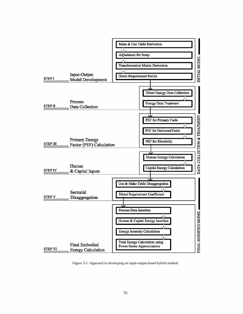
70
Figure 3-1: Approach to developing an input-output-based hybrid method
71
Step II: Collecting data on energy use by industry sectors in physical or energy units for 2002. If the data
were available in monetary units, sector-specific energy prices were used to convert them to energy units.
In addition, if the energy data were in aggregated form, they were decomposed into different fuel
categories (e.g., coal, oil, and natural gas).
Step III: Quantifying PEF for each type of energy delivered for end use to industry sectors. Both the
direct and indirect energy lost and spent in extracting, processing, transmitting, and distributing an energy
source was included.
Step IV: Calculating the energy embodied in human labor and capital inputs using the method
recommended by the literature (e.g. Joshi, 1998). The calculated values were then inserted into the input-
output model as two separate columns similar to the five energy providing sectors of the United States’
economy (based upon Penson, 2012 and 2013 and Dudensing, 2012 and 2013). All energy and nonenergy
inputs to these two sectors were kept at zero to avoid double counting.
Step V: Disaggregating industry sectors manufacturing more than one product using detailed composition
of industry sector inputs and outputs. The sector disaggregation was based on the approach suggested by
Joshi (1998) and Joshi (1999). The disaggregation coefficient used for sectorial inputs are provided in
Table A1-23, Table A1-24, and Table A1-25 in Appendix A1. The process of disaggregation was also
discussed with Penson (2012 and 2013) and Dudensing (2012 and 2013).
Step VI: Applying Power Series Approximation approach to calculate the total embodied energy of study
materials as recommended by Treloar (1998). This approach was preferred against the Leontief’s Inverse
Matrix because it allowed calculating the energy intensities by upstream stages. In addition, the energy
intensities were also calculated fuel wise so that an analysis of the environmental impacts of fuel use can
be performed in the future.
Main Assumptions
Although assumptions are mentioned in the relevant chapters, some assumptions are important to mention
in this section.
While calculating the human energy requirements, it was assumed that all of the energy of food
consumed by an employee was allocated to the employment. It was assumed appropriate to derive
input-output-based energy intensities for sectors producing capital goods in order to quantify
capital energy. The fractions of various capital goods under the categories such as structures,
automobiles, equipment, and software in the total capital investment were used to calculate
weighted average energy intensities.
While calculating the Primary Energy Factors (PEFs) for various energy sources except
electricity, the indirect energy use was calculated using an input-output-based analysis. As most
72
of the energy providing sectors produce only energy goods, their energy intensities were assumed
specific to their primary products. In addition, it was assumed that energy cannot be gained and
any energy gain reported in the year 2002 was ignored.
During the process of sectorial disaggregation, the total purchases of goods by each disaggregated
sector were used to allocate the total input of goods of the aggregated sector. Similarly, the
purchases of services were allocated using each disaggregated sector’s total purchases of services.
The use of commodity by industries was disaggregated based upon each disaggregated
commodity’s share in the total output of the aggregated commodity. In the make table, the make
of disaggregated commodities was assumed same as the aggregated commodity.
While inserting the human and capital inputs, it was assumed that the two represented energy
commodities with no industry sectors producing them. All of the energy and nonenergy inputs to
these commodities were kept at zero.
3.1.4.4 Hypotheses Testing and Result Evaluation
Hypotheses Testing: Three types of information were needed for hypotheses testing: material cost, price,
and embodied energy intensities. As material prices were obtained from multiple sources, it was important
to convert them to the same units. From the review of literature, it was clear that most energy intensities
were given in energy units per mass of materials (e.g. MJ/kg). Some material prices were also given in
units of mass. Therefore, it was decided to convert the embodied energy of each material into energy unit
per unit of its mass. For some material such as steel, cement, and aluminum, the material quantities were
available in mass units, whereas the quantities of materials such as carpets, paint, wood, and bricks were
given in various units such as square foot, gallons, cubic foot, and also in numbers. Appropriate material
density data were sourced and used. As material density was dependent on type of materials used, a
weighted average was derived. For instance, in the case of saw wood, each species of hardwood and
softwood had a different density and it became important to calculate a weighted average density. The
average was weighted on each species’ share in the total wood production. In some cases such as carpets, a
material thickness of 3/8 inch was assumed while calculating the material density.
The cost of a material was interpreted as the total amount of expenditure incurred in manufacturing the
material. Reliable cost data were not readily available and it was considered appropriate to calculate the
material cost. One option to avoid the use of product prices was to gather the total commodity output or
production quantity in physical units. The embodied energy per unit mass then can be calculated using the
following equation:
Equation 3-1
73
Where et, i and Co, i are the total energy intensity of a sector (e.g. MBtu/$) and total sectorial output ($),
respectively. Term Cm, i denotes the total commodity output in physical units (e.g. ton or cubic yards). The
obtained values would provide the total embodied energy Et, i in energy units per mass of the product. To
calculate the cost of a material, its material specific commodity output (in $) was divided by the material
quantities (in physical units such as tons, cubit yards, square foot, etc.). As it avoids use of material prices,
using cost to calculate embodied energy can be more reliable if the cost data are readily available. The
total quantity of a material produced in 2002 was obtained from sources such as historical statistics
provided by the USGS (USGS, 2013) and the Current Industrial Report series published by the USCB
(2002b). However, material quantities were not available for all study materials.
The material prices are volatile and keep changing throughout the year. One way to obtain the average
material prices was to use the material shipments’ quantities and values. These data can be sourced from
the Current Industrial Reports (USCB, 2002b) and also from the 2002 Economic Census (USCB 2002a).
Material prices for most metals and minerals were also available in statistics provided by the USGS
(2013). The missing data were obtained from the 2002 National Construction Estimator (Ogershok, 2002).
Appropriate energy conversion factors were used to convert all prices to comparable units. Some of the
material price and density data used in the study are provided in Table A1-12 and Table A1-15 in
Appendix A1.
Correlation Analysis: The calculated values of embodied energy per unit of mass were analyzed for their
correlation with material prices and costs. A coefficient of determination (r2) less than 0.5, 0.5 - 0.7, 0.7-
0.9 and more than 0.9 is considered to show a weak, moderate, strong, and a very strong positive
correlation, respectively (Ding, 2004; Crawford, 2004; Langston, 2006). According to Taylor (1990) and
Chan (2003), a correlation coefficient (r) less than 0.3 and more than 0.8 indicates a week and strong
positive correlation, respectively. Based on the literature opinion, the following criteria were used in
evaluating the correlation and testing the hypotheses:
Very Weak Weak Moderate Strong Very Strong
r2 <0.3 0.3>r
2 <0.5 0.5>r
2 <0.7 0.7>r
2<0.9 r
2 >0.9
Once a strong correlation was observed, a regression analysis was performed to test the hypotheses. A
regression analysis also helped in deriving an equation for an energy and cost relationship.
Result Evaluation: The input-output-based hybrid method in its current form was not comparable to other
methods due to a varying degree of completeness and specificity. Crawford (2004) noted that evaluations
such as sensitivity and Monte Carlo analysis were not suitable to analyze a method that is a combination of
two entirely different approaches (input-output and process-based). It was also said that the Monte Carlo
analysis is appropriate to evaluate inputs rather than the output (or results) (Crawford, 2004). It was
important to assess the completeness and specificity of the proposed method by comparing its results to
74
relatively incomplete methods such as process-based analyses. Treloar (1998) and Crawford (2004)
recommended using a gap analysis to evaluate the completeness of an input-output-based hybrid method.
The gap analysis assesses the completeness by determining the gap between the proposed method and a
less complete method such as process-based analysis. To assess the reliability of the proposed method, a
comparative analysis was appropriate because it analyzed the correlation between the replaced input-
output values and the inserted process data. The gap and comparative analyses were used in this research
to evaluate the developed method.
Gap Analysis: As the current form of input-output-based method was improved based on the literature
recommendations (e.g., Joshi, 1998; Carter et al., 1981; Treloar, 1998), an input-output analysis was
performed to create a benchmark. In addition, process-based values of embodied energy were collected
from published studies. However, instead of using the process-based values, direct energy process data
were used. As the system boundaries of most of the process data were not clear, it was more appropriate to
analyze the gap with the direct energy intensities. Both the input-output-based and process-based values
were analyzed for their gaps with the input-output-based hybrid values. The gap can be calculated as
(based on Crawford, 2004):
Equation 3-2
Equation 3-3
Where:
Gap between an input-output-based hybrid and process-based embodied energy
Input-output-based hybrid embodied energy
Process-based direct embodied energy
Gap between an input-output-based hybrid and input-output-based embodied energy
Input-output-based embodied energy
Comparative Analysis: As the process energy data were inserted into the input-output model, the inserted
values were compared to the replaced energy values. The comparison was performed by plotting both
values on an x-y plot or by creating a scatter plot. The values then were analyzed for their correlation.
Such comparative analysis provided an assessment of whether or not the process values closely
represented the comparable input-output values. The correlation analysis was performed between the total
energy coefficients of the industry sectors calculated using original input-output data and the comparable
process data. This analysis was also performed for the calculated values of the embodied energy of the
study materials per unit of mass.

75
The calculated values were also compared with the published values of the embodied energy of the study
materials. The purpose of this comparison was to identify if there was any unusual pattern in the calculated
embodied energy values.
3.2 SUMMARY
The research was designed to address the four major issues identified as research gaps. To propose a
complete and consistent system boundary model and a set of embodied energy guidelines, the research
method of LBD was used. As the current version of the input-output-based hybrid method was regarded as
the most appropriate method for calculating the embodied energy, it was used as a basis for making
improvements suggested by literature. The PEF for each energy source used in the United States’ economy
was quantified. The method proposed by Treloar (1998) to avoid the double counting of energy inputs was
used. The human and capital energy was calculated and inserted into the input-output model using the
approach proposed by Joshi (1998). In addition, using the same approach (Joshi, 1998 and Joshi, 1999),
the industry sectors were disaggregated to obtain more study-specific results.
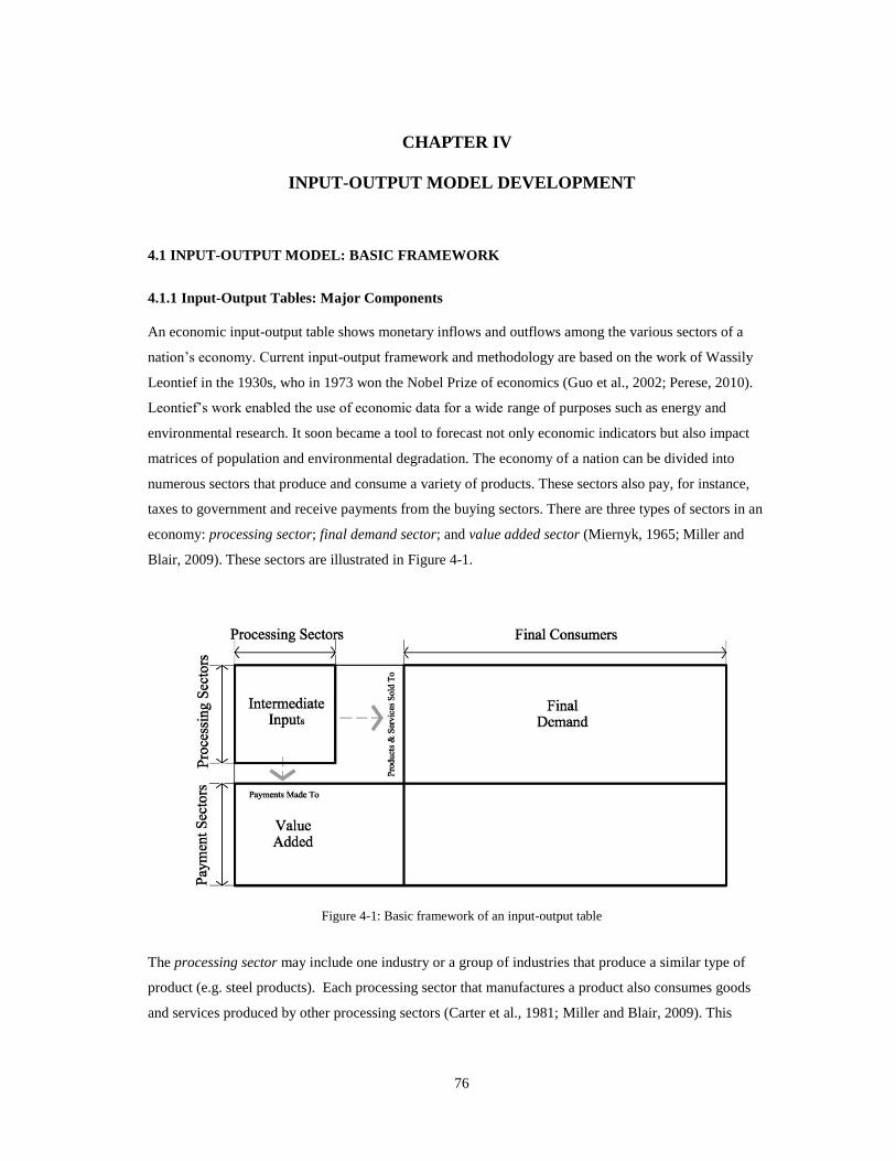
76
CHAPTER IV
INPUT-OUTPUT MODEL DEVELOPMENT
4.
4.1 INPUT-OUTPUT MODEL: BASIC FRAMEWORK
4.1.1 Input-Output Tables: Major Components
An economic input-output table shows monetary inflows and outflows among the various sectors of a
nation’s economy. Current input-output framework and methodology are based on the work of Wassily
Leontief in the 1930s, who in 1973 won the Nobel Prize of economics (Guo et al., 2002; Perese, 2010).
Leontief’s work enabled the use of economic data for a wide range of purposes such as energy and
environmental research. It soon became a tool to forecast not only economic indicators but also impact
matrices of population and environmental degradation. The economy of a nation can be divided into
numerous sectors that produce and consume a variety of products. These sectors also pay, for instance,
taxes to government and receive payments from the buying sectors. There are three types of sectors in an
economy: processing sector; final demand sector; and value added sector (Miernyk, 1965; Miller and
Blair, 2009). These sectors are illustrated in Figure 4-1.
Figure 4-1: Basic framework of an input-output table
The processing sector may include one industry or a group of industries that produce a similar type of
product (e.g. steel products). Each processing sector that manufactures a product also consumes goods
and services produced by other processing sectors (Carter et al., 1981; Miller and Blair, 2009). This
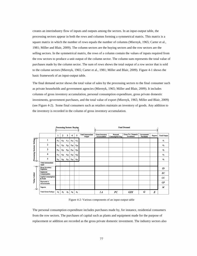
77
creates an interindustry flow of inputs and outputs among the sectors. In an input-output table, the
processing sectors appear in both the rows and columns forming a symmetrical matrix. This matrix is a
square matrix in which the number of rows equals the number of columns (Miernyk, 1965; Carter et al.,
1981; Miller and Blair, 2009). The column sectors are the buying sectors and the row sectors are the
selling sectors. In the symmetrical matrix, the rows of a column contain the values of inputs required from
the row sectors to produce a unit output of the column sector. The column sum represents the total value of
purchases made by the column sector. The sum of rows shows the total output of a row sector that is sold
to the column sectors (Miernyk, 1965; Carter et al., 1981; Miller and Blair, 2009). Figure 4-1 shows the
basic framework of an input-output table.
The final demand sector shows the total value of sales by the processing sectors to the final consumer such
as private households and government agencies (Miernyk, 1965; Miller and Blair, 2009). It includes
columns of gross inventory accumulation, personal consumption expenditure, gross private domestic
investments, government purchases, and the total value of export (Miernyk, 1965; Miller and Blair, 2009)
(see Figure 4-2). Some final consumers such as retailers maintain an inventory of goods. Any addition to
the inventory is recorded in the column of gross inventory accumulation.
Figure 4-2: Various components of an input-output table
The personal consumption expenditure includes purchases made by, for instance, residential consumers
from the row sectors. The purchases of capital such as plants and equipment made for the purpose of
replacement or addition are recorded as the gross private domestic investment. The industry sectors also
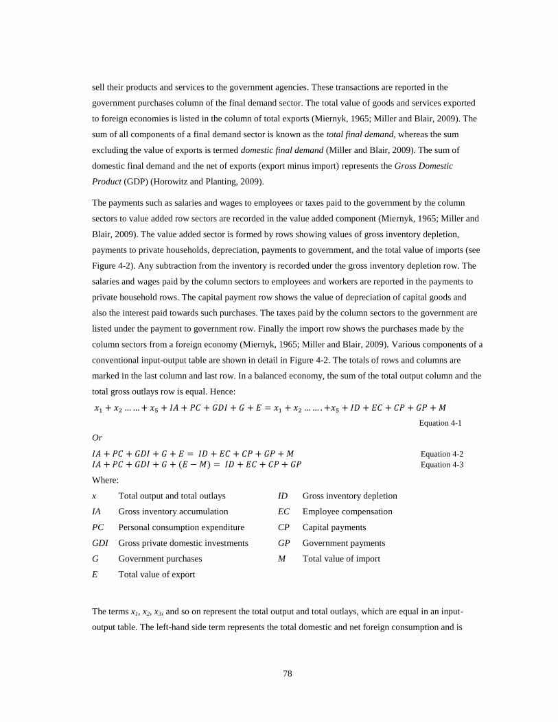
78
sell their products and services to the government agencies. These transactions are reported in the
government purchases column of the final demand sector. The total value of goods and services exported
to foreign economies is listed in the column of total exports (Miernyk, 1965; Miller and Blair, 2009). The
sum of all components of a final demand sector is known as the total final demand, whereas the sum
excluding the value of exports is termed domestic final demand (Miller and Blair, 2009). The sum of
domestic final demand and the net of exports (export minus import) represents the Gross Domestic
Product (GDP) (Horowitz and Planting, 2009).
The payments such as salaries and wages to employees or taxes paid to the government by the column
sectors to value added row sectors are recorded in the value added component (Miernyk, 1965; Miller and
Blair, 2009). The value added sector is formed by rows showing values of gross inventory depletion,
payments to private households, depreciation, payments to government, and the total value of imports (see
Figure 4-2). Any subtraction from the inventory is recorded under the gross inventory depletion row. The
salaries and wages paid by the column sectors to employees and workers are reported in the payments to
private household rows. The capital payment row shows the value of depreciation of capital goods and
also the interest paid towards such purchases. The taxes paid by the column sectors to the government are
listed under the payment to government row. Finally the import row shows the purchases made by the
column sectors from a foreign economy (Miernyk, 1965; Miller and Blair, 2009). Various components of a
conventional input-output table are shown in detail in Figure 4-2. The totals of rows and columns are
marked in the last column and last row. In a balanced economy, the sum of the total output column and the
total gross outlays row is equal. Hence:
Equation 4-1
Or
Equation 4-2
Equation 4-3
Where:
x Total output and total outlays ID Gross inventory depletion
IA Gross inventory accumulation EC Employee compensation
PC Personal consumption expenditure CP Capital payments
GDI Gross private domestic investments GP Government payments
G Government purchases M Total value of import
E Total value of export
The terms x1, x2, x3, and so on represent the total output and total outlays, which are equal in an input-
output table. The left-hand side term represents the total domestic and net foreign consumption and is
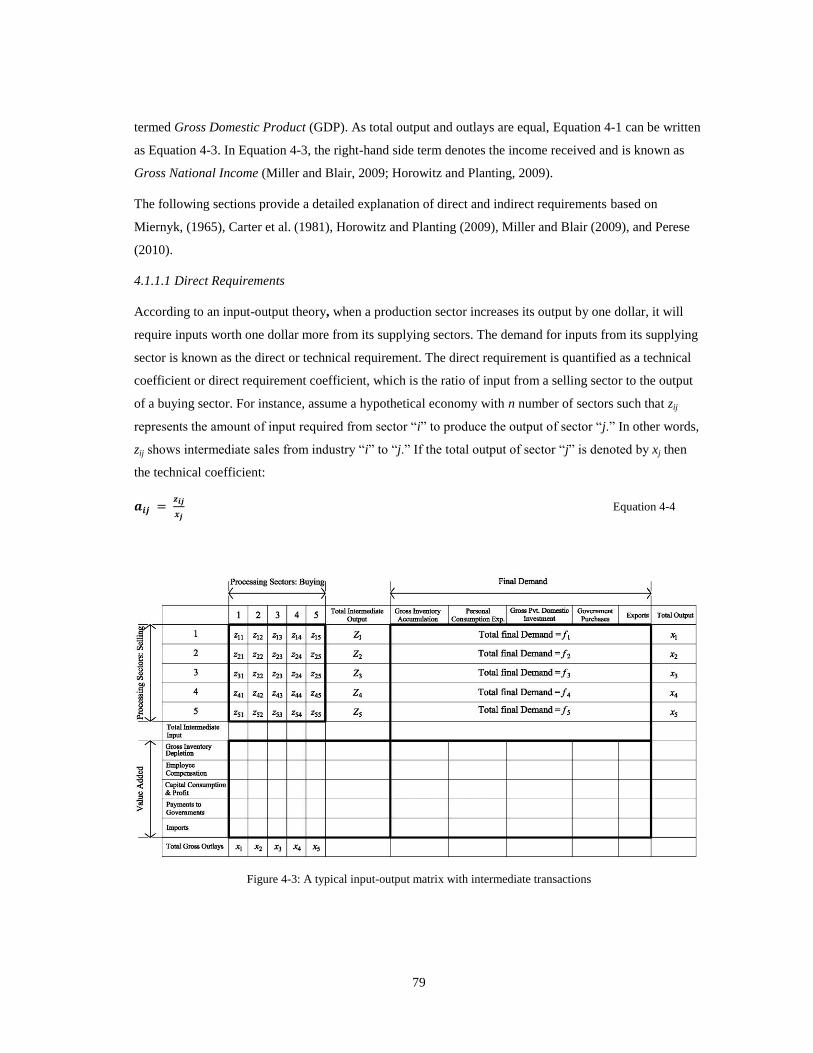
79
termed Gross Domestic Product (GDP). As total output and outlays are equal, Equation 4-1 can be written
as Equation 4-3. In Equation 4-3, the right-hand side term denotes the income received and is known as
Gross National Income (Miller and Blair, 2009; Horowitz and Planting, 2009).
The following sections provide a detailed explanation of direct and indirect requirements based on
Miernyk, (1965), Carter et al. (1981), Horowitz and Planting (2009), Miller and Blair (2009), and Perese
(2010).
4.1.1.1 Direct Requirements
According to an input-output theory, when a production sector increases its output by one dollar, it will
require inputs worth one dollar more from its supplying sectors. The demand for inputs from its supplying
sector is known as the direct or technical requirement. The direct requirement is quantified as a technical
coefficient or direct requirement coefficient, which is the ratio of input from a selling sector to the output
of a buying sector. For instance, assume a hypothetical economy with n number of sectors such that zij
represents the amount of input required from sector “i” to produce the output of sector “j.” In other words,
zij shows intermediate sales from industry “i” to “j.” If the total output of sector “j” is denoted by xj then
the technical coefficient:
Equation 4-4
Figure 4-3: A typical input-output matrix with intermediate transactions
80
In a square matrix of n sectors, each cell contains direct requirement or technical coefficients that
represent the amount of inputs required from row industry by industry at the top of the column to produce
one dollar of column industry’s output. The square matrix shows the interindustry transactions or
intermediate sales of intermediate sectors as shown in Figure 4-3. These sectors buy and sell goods and
services to each other for delivering their outputs to the final demand sector.
It can be seen in Figure 4-3 that the total output of an industry sector is the sum of its total intermediate
sales and its sales to final demand sectors. If inputs from sector “i” to sector “j” are denoted by zij then a
square matrix Z of n sectors would represent the intermediate sales. If x and f represent a column vector of
total output xj and total final demand fj then:
[
] [
] [
]
Equation 4-5
Where “i” is a column vector of only 1s and it is used for summing up the intermediate sales.
4.1.1.2 Indirect Requirements
When an industry sector raises its output by one dollar, it needs to buy more inputs from its supplying
sectors. Each supplying sector also needs to buy more to meet the demand of increased output. Similarly,
supplying sectors of supplying sectors also need to meet the increased demand of their outputs. One can
keep on calculating the increased requirements of inputs by infinite times tracking each input of a
supplying sector. Hence, the impact of increasing output by one dollar can be felt throughout the economy.
This impact represents the indirect requirements. The sum of all requirements due to indirect impact is
known as the indirect requirement, and the respective coefficient is known as the indirect requirement
coefficient. The sum of direct and indirect requirements is the total requirement of a single dollar increase
in a sector’s output. The indirect requirements can be quantified using two approaches: Leontief’s Inverse
Matrix and Power Series Approximation method. In both of the approaches, the direct requirement
coefficients are used as a carrier of indirect impacts.
4.1.2 Leontief’s Inverse Matrix: Direct and Total Requirement Matrix
Equation 4-4 provides the calculation of the direct requirement coefficient. Consider an n-sector square
matrix of direct requirement coefficients:
[
]
If Z and x denote a square matrix of intermediate sales and a vector of total outputs, respectively, then one
can write:
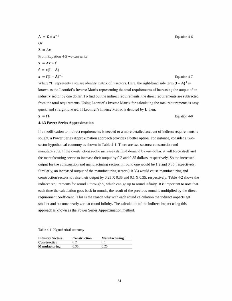
81
Equation 4-6
Or
From Equation 4-5 we can write
Equation 4-7
Where “I” represents a square identity matrix of n sectors. Here, the right-hand side term (I – A)-1
is
known as the Leontief’s Inverse Matrix representing the total requirements of increasing the output of an
industry sector by one dollar. To find out the indirect requirements, the direct requirements are subtracted
from the total requirements. Using Leontief’s Inverse Matrix for calculating the total requirements is easy,
quick, and straightforward. If Leontief’s Inverse Matrix is denoted by L then:
Equation 4-8
4.1.3 Power Series Approximation
If a modification to indirect requirements is needed or a more detailed account of indirect requirements is
sought, a Power Series Approximation approach provides a better option. For instance, consider a two-
sector hypothetical economy as shown in Table 4-1. There are two sectors: construction and
manufacturing. If the construction sector increases its final demand by one dollar, it will force itself and
the manufacturing sector to increase their output by 0.2 and 0.35 dollars, respectively. So the increased
output for the construction and manufacturing sectors in round one would be 1.2 and 0.35, respectively.
Similarly, an increased output of the manufacturing sector (+0.35) would cause manufacturing and
construction sectors to raise their output by 0.25 X 0.35 and 0.1 X 0.35, respectively. Table 4-2 shows the
indirect requirements for round 1 through 5, which can go up to round infinity. It is important to note that
each time the calculation goes back in rounds, the result of the previous round is multiplied by the direct
requirement coefficient. This is the reason why with each round calculation the indirect impacts get
smaller and become nearly zero at round infinity. The calculation of the indirect impact using this
approach is known as the Power Series Approximation method.
Table 4-1: Hypothetical economy
Industry Sectors Construction Manufacturing
Construction 0.2 0.1
Manufacturing 0.35 0.25
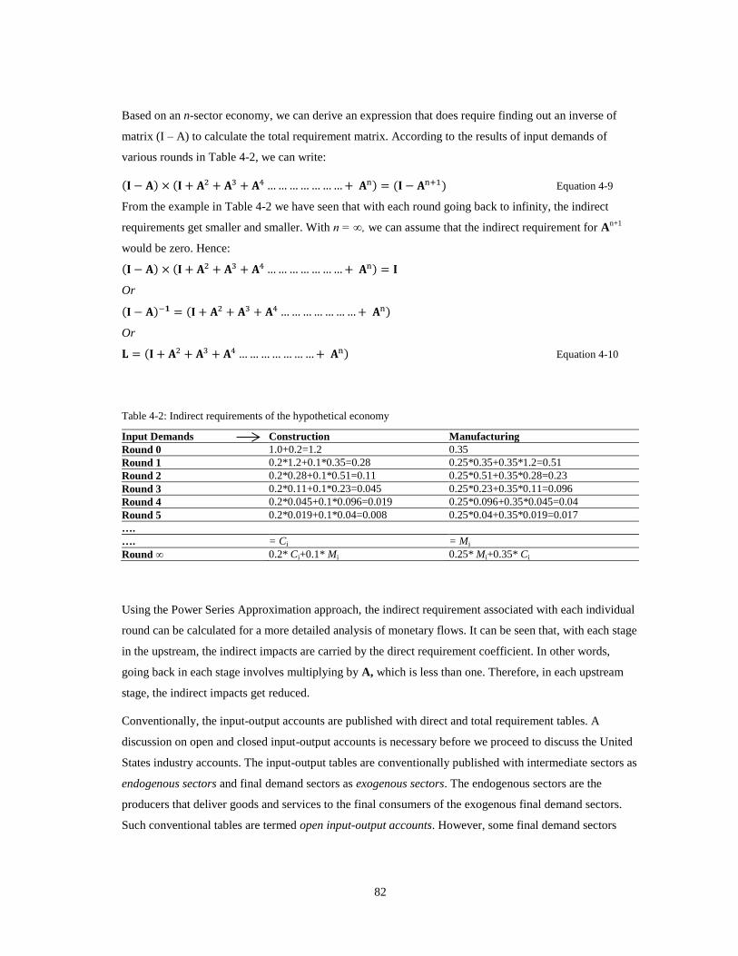
82
Based on an n-sector economy, we can derive an expression that does require finding out an inverse of
matrix (I – A) to calculate the total requirement matrix. According to the results of input demands of
various rounds in Table 4-2, we can write:
Equation 4-9
From the example in Table 4-2 we have seen that with each round going back to infinity, the indirect
requirements get smaller and smaller. With n = ∞, we can assume that the indirect requirement for An+1
would be zero. Hence:
Or
Or
Equation 4-10
Table 4-2: Indirect requirements of the hypothetical economy
Input Demands Construction Manufacturing
Round 0 1.0+0.2=1.2 0.35
Round 1 0.2*1.2+0.1*0.35=0.28 0.25*0.35+0.35*1.2=0.51
Round 2 0.2*0.28+0.1*0.51=0.11 0.25*0.51+0.35*0.28=0.23
Round 3 0.2*0.11+0.1*0.23=0.045 0.25*0.23+0.35*0.11=0.096
Round 4 0.2*0.045+0.1*0.096=0.019 0.25*0.096+0.35*0.045=0.04
Round 5 0.2*0.019+0.1*0.04=0.008 0.25*0.04+0.35*0.019=0.017
….
…. = Ci = Mi
Round ∞ 0.2* Ci+0.1* Mi 0.25* Mi+0.35* Ci
Using the Power Series Approximation approach, the indirect requirement associated with each individual
round can be calculated for a more detailed analysis of monetary flows. It can be seen that, with each stage
in the upstream, the indirect impacts are carried by the direct requirement coefficient. In other words,
going back in each stage involves multiplying by A, which is less than one. Therefore, in each upstream
stage, the indirect impacts get reduced.
Conventionally, the input-output accounts are published with direct and total requirement tables. A
discussion on open and closed input-output accounts is necessary before we proceed to discuss the United
States industry accounts. The input-output tables are conventionally published with intermediate sectors as
endogenous sectors and final demand sectors as exogenous sectors. The endogenous sectors are the
producers that deliver goods and services to the final consumers of the exogenous final demand sectors.
Such conventional tables are termed open input-output accounts. However, some final demand sectors
83
such as private households could be interpreted as intermediate sectors providing labor in return for
receiving salaries and wages. In some economies, one or more of the exogenous final demand sectors are
moved to intermediate sectors, making them endogenous to the economy. Such tables are known as closed
input-output accounts.
4.2 UNITED STATES INPUT-OUTPUT ACCOUNTS
The United States Bureau of Economic Analysis (BEA) reports economic statistics in the form of Annual
Industry Accounts and the Benchmark Input-Output Accounts published every five years (Rassier et al.,
2007; Horowitz and Planting, 2009). These accounts show monetary transactions between various sectors
representing industries, net export (export minus import), value added, and final demand (GDP).
According to Horowitz and Planting (2009), one main purpose of the economic input-output accounts is to
calculate the GDP and Gross National Income of the country. According to Miernyk (1965), the input –
output accounts are used as an “analytical tool” for “economic planning” and for resource allocation and
income distribution. The input-output accounts also help government, industry, business, the research
community, and the public in decision-making and in deriving strategies for the future. For instance, these
accounts can be used for predicting the impact of an increased final demand on the entire economy in
order to identify potential congestion in the input supply. These accounts are also widely used for
quantifying energy flows and resulting greenhouse gas emissions (Miller and Blair, 2009).
The Annual Industry Accounts provide a more aggregated form (65 industries and commodities) of the
flow of goods and services between various industry sectors. The Benchmark Input-Output Accounts that
include 428 commodity sectors and 426 industry sectors present a more detailed form of the flows of
goods and services (Stewart et al., 2007; Rassier et al., 2007). The benchmark accounts are published each
year ending with 2 and 7 (e.g., 1992, 1997, and 2002). Such detailed and comprehensive economic
statistics provide a strong and credible source of information that can be used for the purpose of economic
planning, forecasting, and a variety of other research (Stewart et al., 2007; Rassier et al., 2007). The latest
Benchmark Input-Output Accounts were released in 2007 by BEA for the year 2002 (Stewart et al., 2007).
These accounts were updated in 2008. The BEA publishes the benchmark accounts at a summary and
detailed level. The latest summary level accounts included 133 industries and 135 commodities, whereas
the detailed accounts presented economic data for 426 industries and 428 commodities (Stewart et al.,
2007).
4.2.1 North American Industry Classification System (NAICS)
The industry data are presented by a uniform code system known as the North American Industry
Classification System (NAICS). To improve the comparability of the economic reporting and analysis, the
United States, Canada, and Mexico developed the NAICS under the North American Free Trade

84
Agreement (NAFTA). The NAICS has replaced the earlier 1987 United States Standard Industrial
Classification (SIC) system (Ambler, 1998). The NAICS categorized the industries based on their
production methods. Each industry was denoted by a six-digit NAICS code reading left to right. The first
two digits denoted the sector, the third digit represented the subsector, and the fourth and fifth digits
indicated the industry group and the NAICS industry, respectively (Horowitz and Planting, 2009). Table
4-3 illustrates an example of NAICS classification for iron and steel manufacturing.
Table 4-3: NAICS code example
NAICS Code Description
33 Manufacturing
331 Primary Metal Manufacturing
3311 Iron and Steel Mills and Ferroalloy Manufacturing
33122 Rolling and Drawing of Purchased Steel
331221 Rolled Steel Shape Manufacturing
It is evident from the NAICS that a double-digit classification is more aggregated than a four or six-digit
classification. A six-digit classification is country specific and may not be comparable with other countries
following the NAICS (Horowitz and Planting, 2009). It is also the most detailed categorization available
in the NAICS. According to the NAICS, the United States’ economy is composed of 20 sectors as shown
in Table 4-4 (based on Horowitz and Planting, 2009; USCB, 2002c).
Table 4-4: Sectors of the United States economy as per NAICS
NAICS Sector Description NAICS Sector Description
11 Agriculture, Forestry, Fishing and Hunting 53 Real Estate and Rental and Leasing
21 Mining 54 Professional, Scientific, and Technical Services
22 Utilities 55 Management of Companies and Enterprises
23 Construction 56 Administrative and Support and Waste
Management and Remediation Services
31-33 Manufacturing 61 Educational Services
42 Wholesale Trade 62 Healthcare and Social Assistance
44-45 Retail Trade 71 Arts, Entertainment, and Recreation
48-49 Transportation and Warehousing 72 Accommodation and Food Services
51 Information 81 Other Services (except Public Administration)
52 Finance and Insurance 92 Public Administration
85
4.2.2 Establishments, Industries, and Commodities
According to NAICS, an establishment is a physical location where a group of industries are performing
various industrial operations or providing a range of services. For example, the agriculture sector consists
of various establishments such as farms, ranches, and dairies (USCB, 2002c). Horowitz and Planting
(2009) warned that the terms “establishment” and “enterprise” should not be confused, as they are
different. An enterprise could be a corporation, a company, or an organization that is a legal entity. In
addition, an enterprise may contain one or more establishments (USCB, 2002c; Horowitz and Planting,
2009). An establishment contains one or more industries engaged in numerous activities and using a
similar production method (Stewart et al., 2007; Horowitz and Planting, 2009). However, each industry is
categorized according to its primary activity. The primary activity could be manufacturing a product or
providing a service. The primary activity is determined by the industries’ primary product (goods or
services) that holds the largest share in the production cost, capital investment, or other information such
as revenue, sales, or employment of an establishment (Horowitz and Planting, 2009). In addition to the
primary products, industries also produce or provide other goods or services that are termed secondary
products (Stewart et al., 2007; Horowitz and Planting, 2009).
The goods and services provided by the industries of an establishment are grouped in commodity groups
based on product characteristics. The commodity represents a group of similar goods or similar services
produced or provided by an industry. A commodity could be manufactured or provided by one or more
industries and could be primary or secondary in those industries (Stewart et al., 2007; Horowitz and
Planting, 2009). Hence, the output of a commodity code reports its total output regardless of whether the
commodity is a primary or a secondary product in one or more establishments. In current NAICS,
commodities are categorized by a six-digit NAICS code of industries in which they are primary (Horowitz
and Planting, 2009).
4.2.3 Reclassification and Redefinition
As mentioned earlier, the establishments also produce secondary goods or provide secondary services
other than the primary products. The USBEA treats the secondary products in three ways (based on Guo et
al., 2002; Horowitz and Planting, 2009; Perese, 2010).
4.2.3.1 Reclassification
Under reclassification, the USBEA categorizes a primary product as a secondary product for the purpose
of input-output accounts and reclassifies it to a commodity in which it is primary. Horowitz and Planting
(2009) explained this using the newspaper industry as an example. The United States Census Bureau
(USCB) assigns the newspaper and newspaper advertising both as a primary product. The USBEA,
however, categorizes the newspaper advertising as a secondary product and reclassifies it as a primary

86
product to advertising commodity. When a product is primary to more than one industry due to different
production methods, it is reclassified to a commodity in which it is primary. In the case of reclassification,
only the commodity output changes and the industry output remain unmodified.
4.2.3.2 Redefinition
When the input requirements and structure of a secondary product of an industry differs considerably from
its primary product, the secondary product is redefined to an industry where it is primary. The main
purpose of redefinition is to make the input-product relationship more homogenous. One problem
identified in the past by Bullard and Herendeen (1975), Casler and Wilbur (1984), and Suh and Huppes
(2004) was that of aggregation of primary and secondary products that have a different input structure.
The process of redefinition resolved this problem. In the process of redefinition, only the industry output
changes as the product output is moved across industries. The commodity output remains unchanged after
redefinition.
4.2.3.3 Other Secondary Products
This categorization is done to secondary products that have a similar input structure as the primary product
of an industry. In such a case, the secondary product is included in the output of the primary product. After
this classification neither industry nor commodity output changes.
Two assumptions can be used in the treatment of the secondary product in input-output accounting. The
first assumption is the industry-technology assumption under which a secondary product’s input structure
is identified by the industry that is producing it. Hence, both the primary and secondary products will have
the same inputs under industry-technology assumption. The second assumption is termed the commodity-
technology assumption. Under the commodity-technology assumption, the input structure of a secondary
product is determined from an industry in which the secondary product is primary. Meaning under this
assumption, the primary and secondary products of an industry would not have the same inputs. The
USBEA uses both the assumptions. The commodity-technology assumption is used when secondary
products are redefined, reclassified, or reallocated. The derivation of a symmetrical direct and total
requirement matrix is done based on the industry-technology assumption (Guo et al., 2002; Horowitz and
Planting, 2009; Perese, 2010).
4.2.4 The United States 2002 Benchmark Input-Output Accounts (USBEA, 2008)
The 2002 Benchmark Input-Output Accounts were released in two table formats: Standard and
supplementary tables (Stewart et al., 2007; Horowitz and Planting, 2009). The standard tables provided
industry accounts before redefinition, whereas the supplementary tables reported the industry accounts
after redefinition in addition to other supplemental information. The input-output accounts consist of the
flow of both the primary and secondary goods and services (Stewart et al., 2007; Horowitz and Planting,

87
2009). As supplementary tables provide industry accounts after redefinition, they are used for the purpose
of creating a direct requirement matrix in this research. Three types of supplementary tables are used from
the 2002 benchmark input-output accounts: make table, use table, and the total requirements table. The
following sections describe the three tables (based on Guo et al., 2002; Horowitz and Planting, 2009;
Perese, 2010).
4.2.5 Make and Use Tables
The make table is an Industry-by-commodity table (426 X 430 matrix) that presents production of
commodities by each industry listed by their 6-digit NAICS codes. The rows of the make table show the
industries producing one or more commodities listed at the top of the columns. Hence, the make table is
composed of 426 industry rows and 430 commodity columns. Reading down a column, fractions of a
column commodity produced by the row industries are listed. All of the commodities (of the column)
produced by a row industry can be found reading across the rows. The basic framework of a make table is
shown in Figure 4-4.
Figure 4-4: The make and use table in input-output model
The use table provides a “recipe” for producing a product. It shows the consumption of commodities listed
in rows by the column industries for producing their unit output. The use table is a commodity-by-industry
matrix (430 X 426) of 430 rows and 426 columns. Reading down the column, a composition of input
commodities (in rows) required to produce the output of industries (in columns) can be found. The

88
consumption of a row commodity by column industries can be traced by reading across the rows. The
industries and commodities are listed by their 6-digit NAICS codes.
As industries are conventionally engaged in production of more than one commodity, both the make and
use tables are used to derive a more detailed commodity-by-commodity matrix. The make and use tables
are published before and after redefinition. The 2002 Benchmark Input-Output Accounts were released
with a make table, a use table and a total requirement coefficient table (after redefinition). The total
requirement coefficient table is a commodity-by-commodity matrix (430 X 430) and it provides the total
(direct and indirect) requirements of commodities to produce a unit of each commodity. Reading down the
column, each cell shows the input of the commodity required to produce a unit of the column commodity.
The input-output-based hybrid method of energy analysis requires a commodity-by-commodity direct
requirement coefficient matrix. As the direct requirement matrix is not published with the benchmark
accounts, it needs to be calculated using the raw make and use tables.
4.3 DIRECT REQUIREMENT COEFFICIENT CALCULATION
Guo et al., (2002), Horowitz and Planting (2009), and Perese (2010) provided an approach to calculate a
symmetrical direct and total requirement matrix for the United States’ economy. It is important to note that
detailed make and use tables contain a total of 430 commodities. Unlike the other commodities, scrap,
used and secondhand goods, non-comparable imports, and rest of the world adjustments do not have a
corresponding industry. These commodities appear in the use table but, only scrap and used and
secondhand goods commodities appear in the make table. According to Perese (2010), the rest of the
world adjustments commodity indicates only adjustments to foreign transactions and can be removed from
the calculation. The scrap is not produced by any industry and it is considered a by-product of the process
of fulfilling demands of other industries. Horowitz and Planting (2009) suggested adjustment for scrap
before creating a symmetrical direct requirement matrix so that a demand for scrap does not require an
industry output. The following section explains the steps for creating a direct requirement matrix (based on
Horowitz and Planting, 2009).
Assuming:
V: Industry-by-commodity make matrix (426 X 430)
U: Commodity-by-industry use matrix (430 X 426)
g: Industry output vector (426 X 1); indicates a diagonal matrix of industry outputs
q: Commodity output vector (430 X 1); indicates a diagonal matrix of commodity outputs
s: Scrap vector (426 X 1)
I: Identity matrix
First, a commodity-by-industry direct requirements matrix (use coefficient matrix) is calculated as:
Equation 4-11
89
Second, a matrix showing the market share of industries is derived. The market share matrix (make
coefficient matrix):
Equation 4-12
Next, an adjustment is made to remove the scrap commodity. This is done by calculating industry outputs
without scrap. A vector for the non-scrap ratio is calculated by dividing the industry output excluding
scrap by the total industry output. Each coefficient in the rows of the market share matrix B is then divided
by the non-scrap ratio to make adjustment for scrap. The resulting scrap-adjusted market share matrix is
termed transformation matrix. The industry output vector without scrap:
Equation 4-13
Where s, g, gs, Rs, and W terms are scrap value, industry output vector, industry output vector without
scrap, scrap ratio, and transformation matrix, respectively.
The symmetrical commodity-by-commodity direct requirement matrix can be calculated as:
Equation 4-14
The total requirement matrix can be created by using the Leontief’s Inverse method. The symmetrical
commodity-by-commodity total requirement matrix:
Equation 4-15
For a more detailed analysis of indirect requirements, the Power Series Approximation method can be
applied using direct requirement coefficients.
4.4 SUMMARY
2002 Benchmark Input Output Accounts were used to create a commodity-by-commodity symmetrical
matrix of the direct requirements. First, raw make and use tables were used to create make and use
coefficient matrix, which were then used to derive the direct requirement matrix. All of the data referenced
was after the process of redefinition. An adjustment for scrap was done in the symmetrical matrix as per
the procedure given by Horowitz and Planting (2009).

90
CHAPTER V
ENERGY DATA COLLECTION AND TREATMENT
5.
5.1 PROCESS DATA FOR ENERGY USE BY INDUSTRY SECTORS
The United States’ economy is divided into 20 major sectors that provide goods and services to other
industry sectors and also to final consumers (see also Table 4-4). These sectors are represented by 2-digit
NAICS codes and contain other subsectors denoted by 3-6-digit NAICS codes. The data on energy used
by these sectors were available either in monetary or energy units. Also, the energy consumption by some
sectors was given in an aggregated form under the fuel use or purchased fuel category. Agencies such as
the United States Department of Agriculture (USDA), United States Department of Energy (USDOE),
USCB, and the USGS reported energy use by industry sectors periodically. All of the data available from
diverse sources needed to be collected, disaggregated by fuel use, and converted into energy units.
All establishments classified by the 2002 Annual Energy Review under industrial and commercial sectors
consumed primary (e.g., crude oil) and secondary fuel (e.g., natural gas). Electricity was also purchased to
be used for commercial or industrial operations. The establishments also generated electricity on-site using
the purchased quantities of primary or secondary fuel in Combined Heat and Power (CHP) or electricity
generation plants. A fraction of this on-site generated electricity was consumed by the establishment itself,
the remaining fraction was either sold out or transferred to other establishments within or across sectors.
Figure 5-1 illustrates the energy input and output system of a typical industrial or commercial
establishment. If the net energy consumed by an establishment was included in the calculation, potential
for double counting could exist. For example, the net electricity demand of an establishment represented
the total electrical energy used minus the energy transferred and sold out. As any on-site generation of
energy utilized the purchased quantities of fuel, inclusion of the on-site generated electricity was avoided
in calculating the total energy consumption. If only the purchased quantities of fuel and electricity are
included in the calculation, a potential double counting of energy can be eliminated. In this study, only
quantities that were purchased were included in the calculation. The following sections describe the
energy use data collection and treatment for each major sector.
5.1.1 Energy Consumption: Agriculture Sector (NAICS 11)
The United States agriculture sector is comprised of subsectors involved in two primary operations: crop
production, and animal production. Among the major products delivered by the United States agriculture
sectors are crops, livestock, and poultry. The agriculture sectors consumed energy such as fuel and
electricity directly and indirectly in farm operations related to crop and animal production. The direct
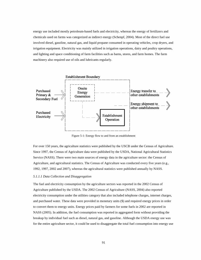
91
energy use included mostly petroleum-based fuels and electricity, whereas the energy of fertilizers and
chemicals used on farms was categorized as indirect energy (Schenpf, 2004). Most of the direct fuel use
involved diesel, gasoline, natural gas, and liquid propane consumed in operating vehicles, crop dryers, and
irrigation equipment. Electricity was mainly utilized in irrigation operations, dairy and poultry operations,
and lighting and space conditioning of farm facilities such as barns, stores, and farm homes. The farm
machinery also required use of oils and lubricants regularly.
Figure 5-1: Energy flow to and from an establishment
For over 150 years, the agriculture statistics were published by the USCB under the Census of Agriculture.
Since 1997, the Census of Agriculture data were published by the USDA, National Agricultural Statistics
Service (NASS). There were two main sources of energy data in the agriculture sector: the Census of
Agriculture, and agricultural statistics. The Census of Agriculture was conducted every five years (e.g.,
1992, 1997, 2002 and 2007), whereas the agricultural statistics were published annually by NASS.
5.1.1.1 Data Collection and Disaggregation
The fuel and electricity consumption by the agriculture sectors was reported in the 2002 Census of
Agriculture published by the USDA. The 2002 Census of Agriculture (NASS, 2004) also reported
electricity consumption under the utilities category that also included telephone charges, internet charges,
and purchased water. These data were provided in monetary units ($) and required energy prices in order
to convert them to energy units. Energy prices paid by farmers for some fuels in 2002 are reported in
NASS (2005). In addition, the fuel consumption was reported in aggregated form without providing the
breakup by individual fuel such as diesel, natural gas, and gasoline. Although the USDA energy use was
for the entire agriculture sector, it could be used to disaggregate the total fuel consumption into energy use
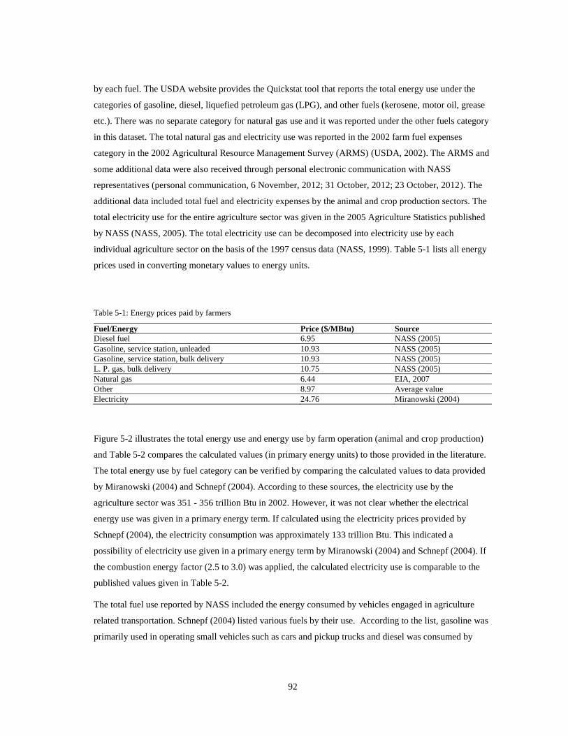
92
by each fuel. The USDA website provides the Quickstat tool that reports the total energy use under the
categories of gasoline, diesel, liquefied petroleum gas (LPG), and other fuels (kerosene, motor oil, grease
etc.). There was no separate category for natural gas use and it was reported under the other fuels category
in this dataset. The total natural gas and electricity use was reported in the 2002 farm fuel expenses
category in the 2002 Agricultural Resource Management Survey (ARMS) (USDA, 2002). The ARMS and
some additional data were also received through personal electronic communication with NASS
representatives (personal communication, 6 November, 2012; 31 October, 2012; 23 October, 2012). The
additional data included total fuel and electricity expenses by the animal and crop production sectors. The
total electricity use for the entire agriculture sector was given in the 2005 Agriculture Statistics published
by NASS (NASS, 2005). The total electricity use can be decomposed into electricity use by each
individual agriculture sector on the basis of the 1997 census data (NASS, 1999). Table 5-1 lists all energy
prices used in converting monetary values to energy units.
Table 5-1: Energy prices paid by farmers
Fuel/Energy Price ($/MBtu) Source
Diesel fuel 6.95 NASS (2005)
Gasoline, service station, unleaded 10.93 NASS (2005)
Gasoline, service station, bulk delivery 10.93 NASS (2005)
L. P. gas, bulk delivery 10.75 NASS (2005)
Natural gas 6.44 EIA, 2007
Other 8.97 Average value
Electricity 24.76 Miranowski (2004)
Figure 5-2 illustrates the total energy use and energy use by farm operation (animal and crop production)
and Table 5-2 compares the calculated values (in primary energy units) to those provided in the literature.
The total energy use by fuel category can be verified by comparing the calculated values to data provided
by Miranowski (2004) and Schnepf (2004). According to these sources, the electricity use by the
agriculture sector was 351 - 356 trillion Btu in 2002. However, it was not clear whether the electrical
energy use was given in a primary energy term. If calculated using the electricity prices provided by
Schnepf (2004), the electricity consumption was approximately 133 trillion Btu. This indicated a
possibility of electricity use given in a primary energy term by Miranowski (2004) and Schnepf (2004). If
the combustion energy factor (2.5 to 3.0) was applied, the calculated electricity use is comparable to the
published values given in Table 5-2.
The total fuel use reported by NASS included the energy consumed by vehicles engaged in agriculture
related transportation. Schnepf (2004) listed various fuels by their use. According to the list, gasoline was
primarily used in operating small vehicles such as cars and pickup trucks and diesel was consumed by
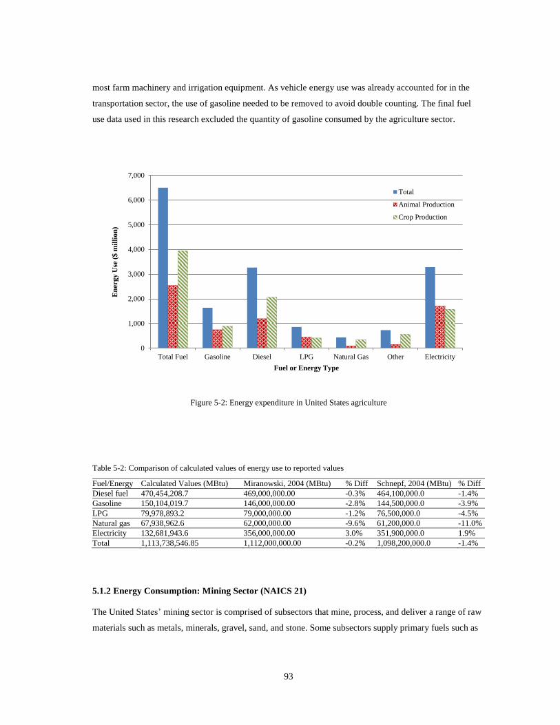
93
most farm machinery and irrigation equipment. As vehicle energy use was already accounted for in the
transportation sector, the use of gasoline needed to be removed to avoid double counting. The final fuel
use data used in this research excluded the quantity of gasoline consumed by the agriculture sector.
Figure 5-2: Energy expenditure in United States agriculture
Table 5-2: Comparison of calculated values of energy use to reported values
Fuel/Energy Calculated Values (MBtu) Miranowski, 2004 (MBtu) % Diff Schnepf, 2004 (MBtu) % Diff
Diesel fuel 470,454,208.7 469,000,000.00 -0.3% 464,100,000.0 -1.4%
Gasoline 150,104,019.7 146,000,000.00 -2.8% 144,500,000.0 -3.9%
LPG 79,978,893.2 79,000,000.00 -1.2% 76,500,000.0 -4.5%
Natural gas 67,938,962.6 62,000,000.00 -9.6% 61,200,000.0 -11.0%
Electricity 132,681,943.6 356,000,000.00 3.0% 351,900,000.0 1.9%
Total 1,113,738,546.85 1,112,000,000.00 -0.2% 1,098,200,000.0 -1.4%
5.1.2 Energy Consumption: Mining Sector (NAICS 21)
The United States’ mining sector is comprised of subsectors that mine, process, and deliver a range of raw
materials such as metals, minerals, gravel, sand, and stone. Some subsectors supply primary fuels such as
0
1,000
2,000
3,000
4,000
5,000
6,000
7,000
Total Fuel Gasoline Diesel LPG Natural Gas Other Electricity
En
erg
y U
se (
$ m
illi
on
)
Fuel or Energy Type
Total
Animal Production
Crop Production

94
coal, oil, and gas that are further processed, converted, or refined into delivered energy products (USDOE,
2007). Mining raw materials involves processes such as extraction, transport, handling, and beneficiation,
which require considerable amount of energy. Most of the extraction processes include digging, drilling,
blasting, ventilation, and dewatering. Material transport and handling processes consume mainly diesel in
vehicle use and electricity in load haul dumps, conveyers, and pumps. Crushing and grinding equipment
such as crushers and mills also use energy. The process of physical and chemical separation of raw
materials is also quite energy intensive. Among the major primary and secondary fuels or energy sources
consumed by the mining sectors are electricity, diesel, natural gas, gasoline, and a mix of other fuels such
as lubricating oil, LPG, and coke.
The mining energy consumption was reported in the industry series of mining published by the Census
Bureau (USCB, 2002a). The energy data were listed under the purchased fuels category for fuels such as
coal, distillate oil, residual oil, gasoline, natural gas and other fuels. Electricity use was provided under
quantity of purchased electricity and quantity of electricity generated less sold category. Mining sectors
also generated electricity on-site and sold a fraction of it. The category of quantity of electricity generated
less sold represented the fraction of on-site generated electricity used by a mining sector. As mentioned
earlier, to avoid double counting, the on-site generated energy was excluded from the total energy
calculation. The purchased fuel category of other fuels denoted a mix of fuels such as LPG and coke.
Another category of purchased fuels was undistributed fuels, which indicated aggregated monetary data
from those establishments that failed to provide detailed fuel use data. The fuel consumption data were
reported either in physical quantity or in monetary units. The electricity use was provided in both physical
and monetary units. The energy use information was published for 29 mining sectors that include metal,
non-metal, fuel, and non-fuel sectors. Among the primary fuel sectors were the oil, gas, and coal
extraction sectors.
The energy use was reported by fuel breakup but in some cases values were withheld due to
confidentiality. The total fuel expenditure was given, which in some cases can be used to estimate the
missing values. To decompose the total fuel expenditure or to derive the missing values, the previous
year’s data can be utilized (Weber et al., 2010). In some cases, data from 2007, 1997, 1992 and 1987 were
used to decompose the total fuel purchased quantity (USCB, 1995; USCB, 1999; USCB, 2004; USCB,
2007). Only the fraction of a fuel as a percentage of the total fuel expenditure was calculated and used to
estimate the missing values. After filling in the missing values using the disaggregation factors, any
difference between the total fuel expenditures before and after filling the missing values was adjusted.
The undistributed fuels were also decomposed using the calculated fractions. Some of the fuels (e.g. coal,
natural gas, etc.) were extracted and used in the same plant. Such fuels were reported separately by the
USCB (2004) and therefore not considered a part of the purchased fuels.
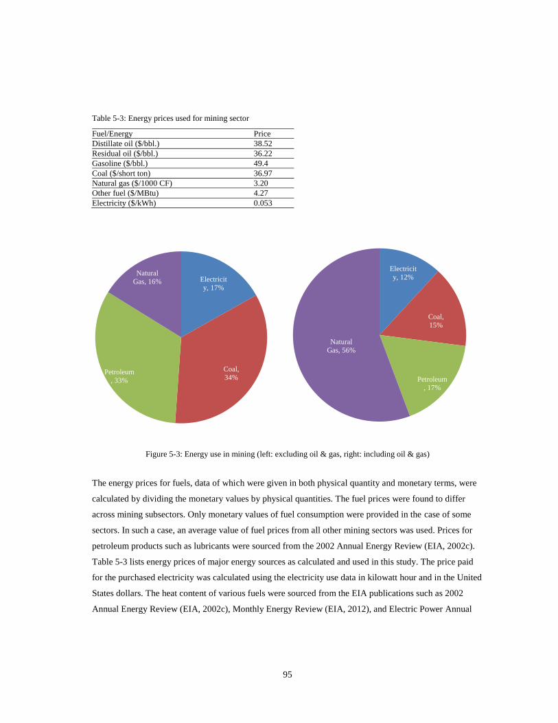
95
Table 5-3: Energy prices used for mining sector
Fuel/Energy Price
Distillate oil ($/bbl.) 38.52
Residual oil ($/bbl.) 36.22
Gasoline ($/bbl.) 49.4
Coal ($/short ton) 36.97
Natural gas ($/1000 CF) 3.20
Other fuel ($/MBtu) 4.27
Electricity ($/kWh) 0.053
Figure 5-3: Energy use in mining (left: excluding oil & gas, right: including oil & gas)
The energy prices for fuels, data of which were given in both physical quantity and monetary terms, were
calculated by dividing the monetary values by physical quantities. The fuel prices were found to differ
across mining subsectors. Only monetary values of fuel consumption were provided in the case of some
sectors. In such a case, an average value of fuel prices from all other mining sectors was used. Prices for
petroleum products such as lubricants were sourced from the 2002 Annual Energy Review (EIA, 2002c).
Table 5-3 lists energy prices of major energy sources as calculated and used in this study. The price paid
for the purchased electricity was calculated using the electricity use data in kilowatt hour and in the United
States dollars. The heat content of various fuels were sourced from the EIA publications such as 2002
Annual Energy Review (EIA, 2002c), Monthly Energy Review (EIA, 2012), and Electric Power Annual
Electricit
y, 17%
Coal,
34%
Petroleum
, 33%
Natural
Gas, 16%
Electricit
y, 12%
Coal,
15%
Petroleum
, 17%
Natural
Gas, 56%
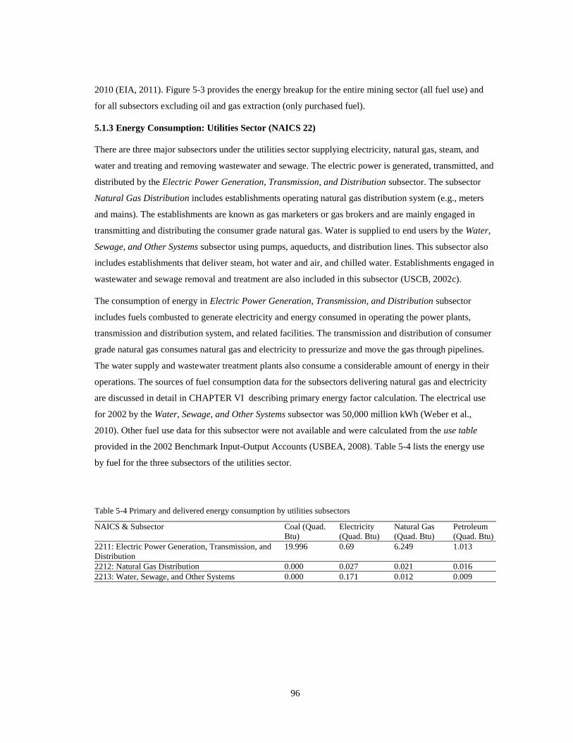
96
2010 (EIA, 2011). Figure 5-3 provides the energy breakup for the entire mining sector (all fuel use) and
for all subsectors excluding oil and gas extraction (only purchased fuel).
5.1.3 Energy Consumption: Utilities Sector (NAICS 22)
There are three major subsectors under the utilities sector supplying electricity, natural gas, steam, and
water and treating and removing wastewater and sewage. The electric power is generated, transmitted, and
distributed by the Electric Power Generation, Transmission, and Distribution subsector. The subsector
Natural Gas Distribution includes establishments operating natural gas distribution system (e.g., meters
and mains). The establishments are known as gas marketers or gas brokers and are mainly engaged in
transmitting and distributing the consumer grade natural gas. Water is supplied to end users by the Water,
Sewage, and Other Systems subsector using pumps, aqueducts, and distribution lines. This subsector also
includes establishments that deliver steam, hot water and air, and chilled water. Establishments engaged in
wastewater and sewage removal and treatment are also included in this subsector (USCB, 2002c).
The consumption of energy in Electric Power Generation, Transmission, and Distribution subsector
includes fuels combusted to generate electricity and energy consumed in operating the power plants,
transmission and distribution system, and related facilities. The transmission and distribution of consumer
grade natural gas consumes natural gas and electricity to pressurize and move the gas through pipelines.
The water supply and wastewater treatment plants also consume a considerable amount of energy in their
operations. The sources of fuel consumption data for the subsectors delivering natural gas and electricity
are discussed in detail in CHAPTER VI describing primary energy factor calculation. The electrical use
for 2002 by the Water, Sewage, and Other Systems subsector was 50,000 million kWh (Weber et al.,
2010). Other fuel use data for this subsector were not available and were calculated from the use table
provided in the 2002 Benchmark Input-Output Accounts (USBEA, 2008). Table 5-4 lists the energy use
by fuel for the three subsectors of the utilities sector.
Table 5-4 Primary and delivered energy consumption by utilities subsectors
NAICS & Subsector Coal (Quad.
Btu)
Electricity
(Quad. Btu)
Natural Gas
(Quad. Btu)
Petroleum
(Quad. Btu)
2211: Electric Power Generation, Transmission, and
Distribution
19.996 0.69 6.249 1.013
2212: Natural Gas Distribution 0.000 0.027 0.021 0.016
2213: Water, Sewage, and Other Systems 0.000 0.171 0.012 0.009
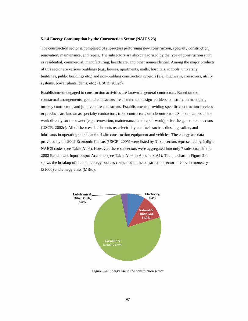
97
5.1.4 Energy Consumption by the Construction Sector (NAICS 23)
The construction sector is comprised of subsectors performing new construction, specialty construction,
renovation, maintenance, and repair. The subsectors are also categorized by the type of construction such
as residential, commercial, manufacturing, healthcare, and other nonresidential. Among the major products
of this sector are various buildings (e.g., houses, apartments, malls, hospitals, schools, university
buildings, public buildings etc.) and non-building construction projects (e.g., highways, crossovers, utility
systems, power plants, dams, etc.) (USCB, 2002c).
Establishments engaged in construction activities are known as general contractors. Based on the
contractual arrangements, general contractors are also termed design-builders, construction managers,
turnkey contractors, and joint venture contractors. Establishments providing specific construction services
or products are known as specialty contractors, trade contractors, or subcontractors. Subcontractors either
work directly for the owner (e.g., renovation, maintenance, and repair work) or for the general contractors
(USCB, 2002c). All of these establishments use electricity and fuels such as diesel, gasoline, and
lubricants in operating on-site and off-site construction equipment and vehicles. The energy use data
provided by the 2002 Economic Census (USCB, 2005) were listed by 31 subsectors represented by 6-digit
NAICS codes (see Table A1-6). However, these subsectors were aggregated into only 7 subsectors in the
2002 Benchmark Input-output Accounts (see Table A1-6 in Appendix A1). The pie chart in Figure 5-4
shows the breakup of the total energy sources consumed in the construction sector in 2002 in monetary
($1000) and energy units (MBtu).
Figure 5-4: Energy use in the construction sector
Electricity,
8.3%
Natural &
Other Gas,
11.9%
Gasoline &
Diesel, 76.4%
Lubricants &
Other Fuels,
3.4%
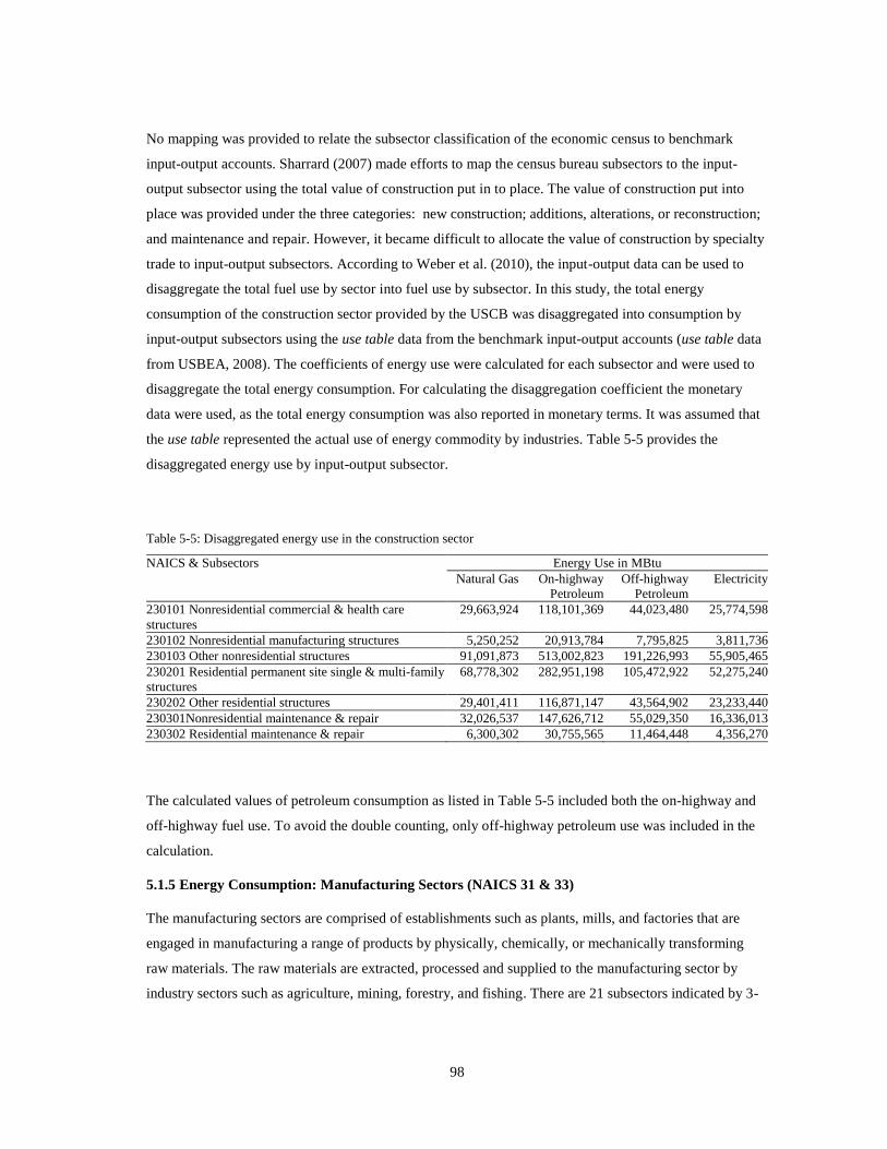
98
No mapping was provided to relate the subsector classification of the economic census to benchmark
input-output accounts. Sharrard (2007) made efforts to map the census bureau subsectors to the input-
output subsector using the total value of construction put in to place. The value of construction put into
place was provided under the three categories: new construction; additions, alterations, or reconstruction;
and maintenance and repair. However, it became difficult to allocate the value of construction by specialty
trade to input-output subsectors. According to Weber et al. (2010), the input-output data can be used to
disaggregate the total fuel use by sector into fuel use by subsector. In this study, the total energy
consumption of the construction sector provided by the USCB was disaggregated into consumption by
input-output subsectors using the use table data from the benchmark input-output accounts (use table data
from USBEA, 2008). The coefficients of energy use were calculated for each subsector and were used to
disaggregate the total energy consumption. For calculating the disaggregation coefficient the monetary
data were used, as the total energy consumption was also reported in monetary terms. It was assumed that
the use table represented the actual use of energy commodity by industries. Table 5-5 provides the
disaggregated energy use by input-output subsector.
Table 5-5: Disaggregated energy use in the construction sector
NAICS & Subsectors Energy Use in MBtu
Natural Gas On-highway
Petroleum
Off-highway
Petroleum
Electricity
230101 Nonresidential commercial & health care
structures
29,663,924 118,101,369 44,023,480 25,774,598
230102 Nonresidential manufacturing structures 5,250,252 20,913,784 7,795,825 3,811,736
230103 Other nonresidential structures 91,091,873 513,002,823 191,226,993 55,905,465
230201 Residential permanent site single & multi-family
structures
68,778,302 282,951,198 105,472,922 52,275,240
230202 Other residential structures 29,401,411 116,871,147 43,564,902 23,233,440
230301Nonresidential maintenance & repair 32,026,537 147,626,712 55,029,350 16,336,013
230302 Residential maintenance & repair 6,300,302 30,755,565 11,464,448 4,356,270
The calculated values of petroleum consumption as listed in Table 5-5 included both the on-highway and
off-highway fuel use. To avoid the double counting, only off-highway petroleum use was included in the
calculation.
5.1.5 Energy Consumption: Manufacturing Sectors (NAICS 31 & 33)
The manufacturing sectors are comprised of establishments such as plants, mills, and factories that are
engaged in manufacturing a range of products by physically, chemically, or mechanically transforming
raw materials. The raw materials are extracted, processed and supplied to the manufacturing sector by
industry sectors such as agriculture, mining, forestry, and fishing. There are 21 subsectors indicated by 3-
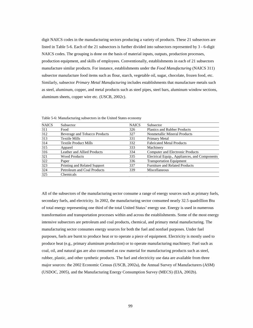
99
digit NAICS codes in the manufacturing sectors producing a variety of products. These 21 subsectors are
listed in Table 5-6. Each of the 21 subsectors is further divided into subsectors represented by 3 - 6-digit
NAICS codes. The grouping is done on the basis of material inputs, outputs, production processes,
production equipment, and skills of employees. Conventionally, establishments in each of 21 subsectors
manufacture similar products. For instance, establishments under the Food Manufacturing (NAICS 311)
subsector manufacture food items such as flour, starch, vegetable oil, sugar, chocolate, frozen food, etc.
Similarly, subsector Primary Metal Manufacturing includes establishments that manufacture metals such
as steel, aluminum, copper, and metal products such as steel pipes, steel bars, aluminum window sections,
aluminum sheets, copper wire etc. (USCB, 2002c).
Table 5-6: Manufacturing subsectors in the United States economy
NAICS Subsector NAICS Subsector
311 Food 326 Plastics and Rubber Products
312 Beverage and Tobacco Products 327 Nonmetallic Mineral Products
313 Textile Mills 331 Primary Metal
314 Textile Product Mills 332 Fabricated Metal Products
315 Apparel 333 Machinery
316 Leather and Allied Products 334 Computer and Electronic Products
321 Wood Products 335 Electrical Equip., Appliances, and Components
322 Paper 336 Transportation Equipment
323 Printing and Related Support 337 Furniture and Related Products
324 Petroleum and Coal Products 339 Miscellaneous
325 Chemicals
All of the subsectors of the manufacturing sector consume a range of energy sources such as primary fuels,
secondary fuels, and electricity. In 2002, the manufacturing sector consumed nearly 32.5 quadrillion Btu
of total energy representing one third of the total United States’ energy use. Energy is used in numerous
transformation and transportation processes within and across the establishments. Some of the most energy
intensive subsectors are petroleum and coal products, chemical, and primary metal manufacturing. The
manufacturing sector consumes energy sources for both the fuel and nonfuel purposes. Under fuel
purposes, fuels are burnt to produce heat or to operate a piece of equipment. Electricity is mostly used to
produce heat (e.g., primary aluminum production) or to operate manufacturing machinery. Fuel such as
coal, oil, and natural gas are also consumed as raw material for manufacturing products such as steel,
rubber, plastic, and other synthetic products. The fuel and electricity use data are available from three
major sources: the 2002 Economic Census (USCB, 2002a), the Annual Survey of Manufacturers (ASM)
(USDOC, 2005), and the Manufacturing Energy Consumption Survey (MECS) (EIA, 2002b).

100
The fuel consumption for the manufacturing subsectors (by 6-digit NAICS codes) was reported in the
2002 Economic Census performed every five years by the United States Census Bureau. However, the fuel
use was provided in an aggregated form and in monetary units as fuel purchased. The fuel and electricity
use information was also published in the ASM by the United States Department of Commerce,
Economics and Statistics Administration. The electricity use was reported in both the monetary units and
physical units (kWh). ASM also reported the amount of net electricity generated on-site (total electricity
generated less sold). It should be noted that only fuels that are purchased were reported in the ASM and
any amount of energy (e.g., biomass, waste, by-product fuel) that is generated on-site may not be included
in the reported value. Another source of fuel and electricity consumption data was the 2002 Manufacturing
Energy Consumption Survey (MECS) administered by the United States Department of Energy (USDOE),
Energy Information Administration (EIA) (EIA, 2002b). Although the MECS data were reported by
individual fuel use in both the physical and energy units, energy use for only the major sectors (by 3, 4, 5,
6-digit NAICS codes) was reported.
Four types of energy data are published by the EIA in the 2002 MECS (EIA, 2002b). Table 5-7 illustrates
the types of data with the energy components reported in the MECS data. The first type of energy data
referred was First Use for All Purposes. In this type of energy data, all fuel and nonfuel use of energy was
reported except the use of any energy produced on-site from energy inputs. It also reported the amount of
energy shipped to other establishments. Energy data type Energy Use for Fuel Purposes listed quantities
of all energy produced on-site or off-site from energy or nonenergy inputs consumed as a fuel.
Consumption of energy produced off-site for nonfuel purposes was included in the third energy data type
Energy Use for Nonfuel Purposes. It also included the nonfuel use of energy produced on-site from
nonenergy inputs. The nonfuel use of energy generated on-site from energy sources was not reported in
any of the three data types. If Energy Use for Fuel Purposes and Energy Use for Nonfuel Purposes are
summed, the total would include all energy that is consumed on-site for fuel and nonfuel purposes. In
order to estimate the amount of energy generated on-site from energy sources and used as a fuel, First Use
for All Purposes should be subtracted from the total of Energy Use for Fuel Purposes and Energy Use for
Nonfuel Purposes.
For calculating the total energy use, the category First Use for All Purposes is used, as it excludes all on-
site energy consumed on-site, transferred, or sold out.
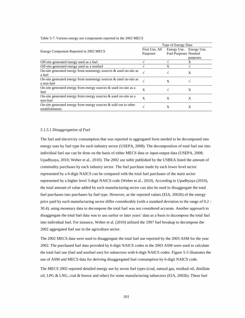
101
Table 5-7: Various energy use components reported in the 2002 MECS
Energy Component Reported in 2002 MECS
Type of Energy Data
First Use, All
Purposes
Energy Use,
Fuel Purposes
Energy Use,
Nonfuel
purposes
Off-site generated energy used as a fuel √ √ X
Off-site generated energy used as a nonfuel √ X √
On-site generated energy from nonenergy sources & used on-site as
a fuel √ √ X
On-site generated energy from nonenergy sources & used on-site as
a non-fuel √ X √
On-site generated energy from energy sources & used on-site as a
fuel X √ X
On-site generated energy from energy sources & used on-site as a
non-fuel X X X
On-site generated energy from energy sources & sold out to other
establishments √ X X
5.1.5.1 Disaggregation of Fuel
The fuel and electricity consumption that was reported in aggregated form needed to be decomposed into
energy uses by fuel type for each industry sector (USEPA, 2008). The decomposition of total fuel use into
individual fuel use can be done on the basis of either MECS data or input-output data (USEPA, 2008;
Upadhyaya, 2010; Weber et al., 2010). The 2002 use table published by the USBEA listed the amount of
commodity purchases by each industry sector. The fuel purchase made by each lower level sector
represented by a 6-digit NAICS can be compared with the total fuel purchases of the main sector
represented by a higher level 3-digit NAICS code (Weber et al., 2010). According to Upadhyaya (2010),
the total amount of value added by each manufacturing sector can also be used to disaggregate the total
fuel purchases into purchases by fuel type. However, as the reported values (EIA, 2002b) of the energy
price paid by each manufacturing sector differ considerably (with a standard deviation in the range of 0.2 -
30.4), using monetary data to decompose the total fuel was not considered accurate. Another approach to
disaggregate the total fuel data was to use earlier or later years’ data as a basis to decompose the total fuel
into individual fuel. For instance, Weber et al. (2010) utilized the 1997 fuel breakup to decompose the
2002 aggregated fuel use in the agriculture sector.
The 2002 MECS data were used to disaggregate the total fuel use reported by the 2003 ASM for the year
2002. The purchased fuel data provided by 6-digit NAICS codes in the 2003 ASM were used to calculate
the total fuel use (fuel and nonfuel use) for subsectors with 6-digit NAICS codes. Figure 5-5 illustrates the
use of ASM and MECS data for deriving disaggregated fuel consumption by 6-digit NAICS code.
The MECS 2002 reported detailed energy use by seven fuel types (coal, natural gas, residual oil, distillate
oil, LPG & LNG, coal & breeze and other) for some manufacturing subsectors (EIA, 2002b). These fuel
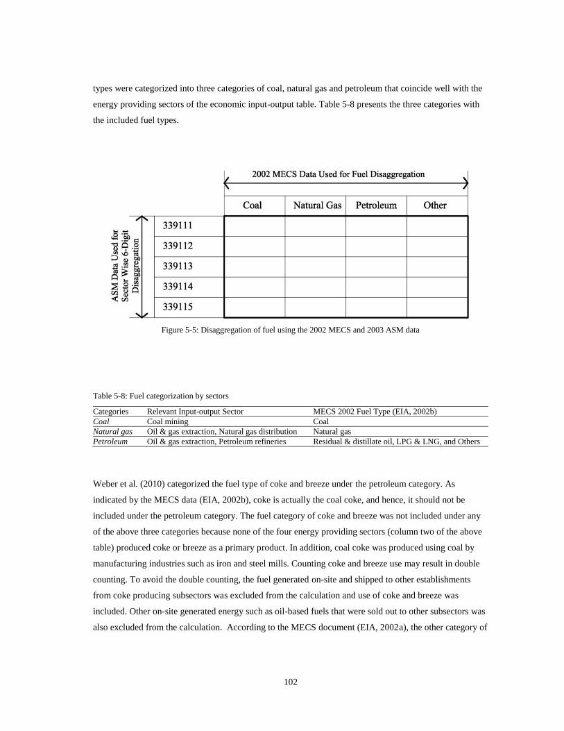
102
types were categorized into three categories of coal, natural gas and petroleum that coincide well with the
energy providing sectors of the economic input-output table. Table 5-8 presents the three categories with
the included fuel types.
Figure 5-5: Disaggregation of fuel using the 2002 MECS and 2003 ASM data
Table 5-8: Fuel categorization by sectors
Categories Relevant Input-output Sector MECS 2002 Fuel Type (EIA, 2002b)
Coal Coal mining Coal
Natural gas Oil & gas extraction, Natural gas distribution Natural gas
Petroleum Oil & gas extraction, Petroleum refineries Residual & distillate oil, LPG & LNG, and Others
Weber et al. (2010) categorized the fuel type of coke and breeze under the petroleum category. As
indicated by the MECS data (EIA, 2002b), coke is actually the coal coke, and hence, it should not be
included under the petroleum category. The fuel category of coke and breeze was not included under any
of the above three categories because none of the four energy providing sectors (column two of the above
table) produced coke or breeze as a primary product. In addition, coal coke was produced using coal by
manufacturing industries such as iron and steel mills. Counting coke and breeze use may result in double
counting. To avoid the double counting, the fuel generated on-site and shipped to other establishments
from coke producing subsectors was excluded from the calculation and use of coke and breeze was
included. Other on-site generated energy such as oil-based fuels that were sold out to other subsectors was
also excluded from the calculation. According to the MECS document (EIA, 2002a), the other category of
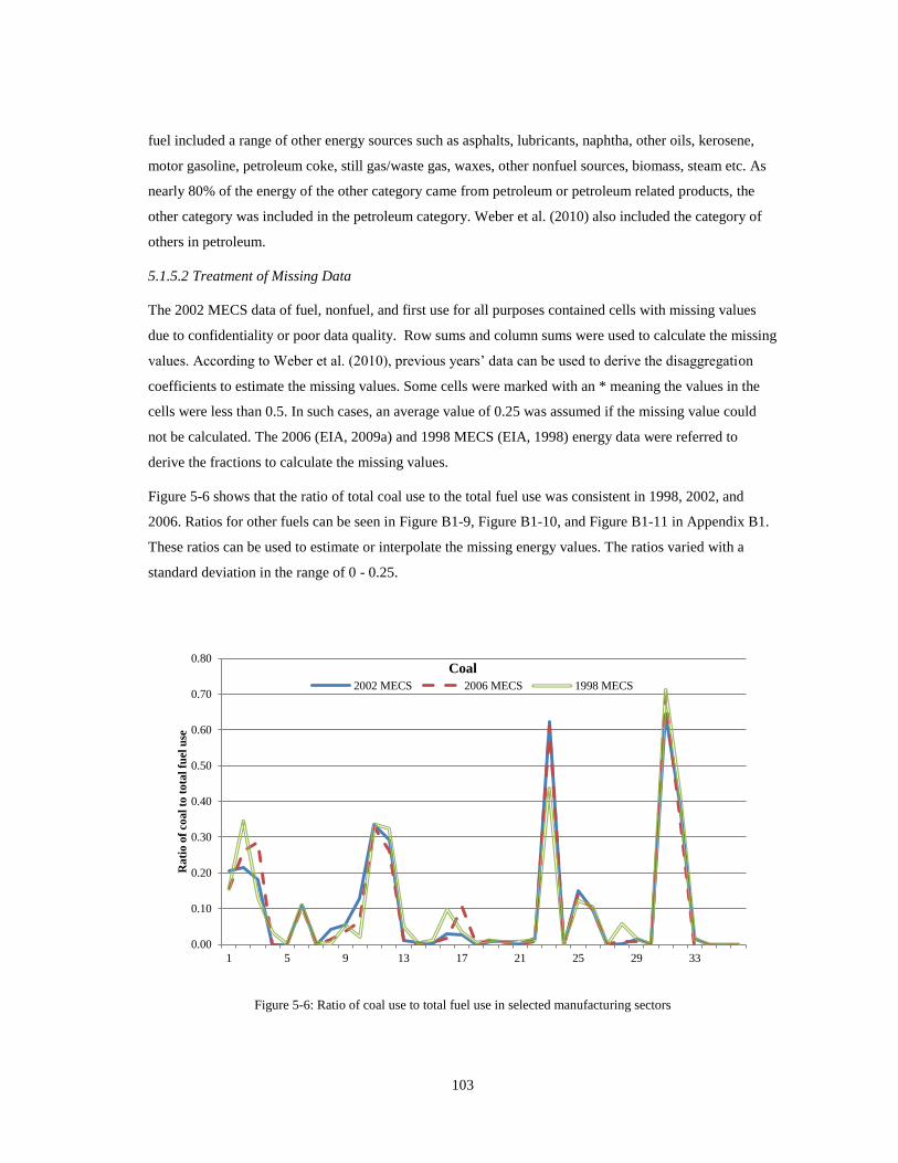
103
fuel included a range of other energy sources such as asphalts, lubricants, naphtha, other oils, kerosene,
motor gasoline, petroleum coke, still gas/waste gas, waxes, other nonfuel sources, biomass, steam etc. As
nearly 80% of the energy of the other category came from petroleum or petroleum related products, the
other category was included in the petroleum category. Weber et al. (2010) also included the category of
others in petroleum.
5.1.5.2 Treatment of Missing Data
The 2002 MECS data of fuel, nonfuel, and first use for all purposes contained cells with missing values
due to confidentiality or poor data quality. Row sums and column sums were used to calculate the missing
values. According to Weber et al. (2010), previous years’ data can be used to derive the disaggregation
coefficients to estimate the missing values. Some cells were marked with an * meaning the values in the
cells were less than 0.5. In such cases, an average value of 0.25 was assumed if the missing value could
not be calculated. The 2006 (EIA, 2009a) and 1998 MECS (EIA, 1998) energy data were referred to
derive the fractions to calculate the missing values.
Figure 5-6 shows that the ratio of total coal use to the total fuel use was consistent in 1998, 2002, and
2006. Ratios for other fuels can be seen in Figure B1-9, Figure B1-10, and Figure B1-11 in Appendix B1.
These ratios can be used to estimate or interpolate the missing energy values. The ratios varied with a
standard deviation in the range of 0 - 0.25.
Figure 5-6: Ratio of coal use to total fuel use in selected manufacturing sectors
0.00
0.10
0.20
0.30
0.40
0.50
0.60
0.70
0.80
1 5 9 13 17 21 25 29 33
Ra
tio
of
co
al
to t
ota
l fu
el
use
Coal
2002 MECS 2006 MECS 1998 MECS
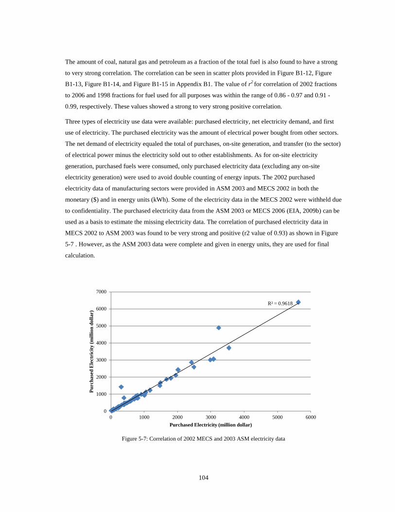
104
The amount of coal, natural gas and petroleum as a fraction of the total fuel is also found to have a strong
to very strong correlation. The correlation can be seen in scatter plots provided in Figure B1-12, Figure
B1-13, Figure B1-14, and Figure B1-15 in Appendix B1. The value of r2 for correlation of 2002 fractions
to 2006 and 1998 fractions for fuel used for all purposes was within the range of 0.86 - 0.97 and 0.91 -
0.99, respectively. These values showed a strong to very strong positive correlation.
Three types of electricity use data were available: purchased electricity, net electricity demand, and first
use of electricity. The purchased electricity was the amount of electrical power bought from other sectors.
The net demand of electricity equaled the total of purchases, on-site generation, and transfer (to the sector)
of electrical power minus the electricity sold out to other establishments. As for on-site electricity
generation, purchased fuels were consumed, only purchased electricity data (excluding any on-site
electricity generation) were used to avoid double counting of energy inputs. The 2002 purchased
electricity data of manufacturing sectors were provided in ASM 2003 and MECS 2002 in both the
monetary ($) and in energy units (kWh). Some of the electricity data in the MECS 2002 were withheld due
to confidentiality. The purchased electricity data from the ASM 2003 or MECS 2006 (EIA, 2009b) can be
used as a basis to estimate the missing electricity data. The correlation of purchased electricity data in
MECS 2002 to ASM 2003 was found to be very strong and positive (r2 value of 0.93) as shown in Figure
5-7 . However, as the ASM 2003 data were complete and given in energy units, they are used for final
calculation.
Figure 5-7: Correlation of 2002 MECS and 2003 ASM electricity data
R² = 0.9618
0
1000
2000
3000
4000
5000
6000
7000
0 1000 2000 3000 4000 5000 6000
Pu
rch
ase
d E
lectr
icit
y (
mil
lio
n d
oll
ar)
Purchased Electricity (million dollar)
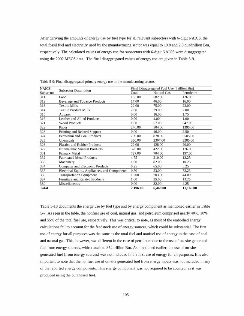
105
After deriving the amounts of energy use by fuel type for all relevant subsectors with 6-digit NAICS, the
total fossil fuel and electricity used by the manufacturing sector was equal to 19.8 and 2.8 quadrillion Btu,
respectively. The calculated values of energy use for subsectors with 6-digit NAICS were disaggregated
using the 2002 MECS data. The final disaggregated values of energy use are given in Table 5-9.
Table 5-9: Final disaggregated primary energy use in the manufacturing sectors
NAICS
Subsector Subsector Description
Final Disaggregated Fuel Use (Trillion Btu)
Coal Natural Gas Petroleum
311 Food 185.00 582.00 126.00
312 Beverage and Tobacco Products 17.00 46.00 16.00
313 Textile Mills 22.00 75.00 23.00
314 Textile Product Mills 7.00 29.00 7.00
315 Apparel 0.00 16.00 1.75
316 Leather and Allied Products 0.00 4.00 1.00
321 Wood Products 1.00 57.00 247.00
322 Paper 240.00 504.00 1395.00
323 Printing and Related Support 0.00 46.00 2.50
324 Petroleum and Coal Products 289.00 878.00 5505.00
325 Chemicals 350.00 2307.00 3285.00
326 Plastics and Rubber Products 22.00 128.00 20.00
327 Nonmetallic Mineral Products 320.00 422.00 176.00
331 Primary Metal 727.00 704.00 197.00
332 Fabricated Metal Products 4.75 210.00 12.25
333 Machinery 1.00 82.00 10.25
334 Computer and Electronic Products 0.25 65.00 5.25
335 Electrical Equip., Appliances, and Components 0.50 53.00 72.25
336 Transportation Equipment 10.00 203.00 44.00
337 Furniture and Related Products 1.00 25.00 13.25
339 Miscellaneous 0.00 32.00 4.25
Total 2,196.00 6,468.00 11,165.00
Table 5-10 documents the energy use by fuel type and by energy component as mentioned earlier in Table
5-7. As seen in the table, the nonfuel use of coal, natural gas, and petroleum comprised nearly 40%, 10%,
and 55% of the total fuel use, respectively. This was critical to note, as most of the embodied energy
calculations fail to account for the feedstock use of energy sources, which could be substantial. The first
use of energy for all purposes was the same as the total fuel and nonfuel use of energy in the case of coal
and natural gas. This, however, was different in the case of petroleum due to the use of on-site generated
fuel from energy sources, which totals to 854 trillion Btu. As mentioned earlier, the use of on-site
generated fuel (from energy sources) was not included in the first use of energy for all purposes. It is also
important to note that the nonfuel use of on-site generated fuel from energy inputs was not included in any
of the reported energy components. This energy component was not required to be counted, as it was
produced using the purchased fuel.
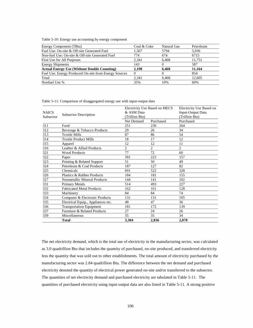
106
Table 5-10: Energy use accounting by energy component
Energy Component (TBtu) Coal & Coke Natural Gas Petroleum
Fuel Use: On-site & Off-site Generated Fuel 1,567 5794 5,036
Non-fuel Use: On-site & Off-site Generated Fuel 774 674 6715
First Use for All Purposes 2,341 6,468 11,751
Energy Shipments 143 0 587
Actual Energy Use (Without Double Counting) 2,198 6,468 11,164
Fuel Use: Energy Produced On-site from Energy Sources 0 0 854
Total 2,341 6,468 12,605
Nonfuel Use % 35% 10% 60%
Table 5-11: Comparison of disaggregated energy use with input-output data
NAICS
Subsector Subsector Description
Electricity Use Based on MECS
& ASM Data
(Trillion Btu)
Electricity Use Based on
Input-Output Data
(Trillion Btu)
Net Demand Purchased Purchased
311 Food 251 230 264
312 Beverage & Tobacco Products 29 26 34
313 Textile Mills 87 86 54
314 Textile Product Mills 18 17 12
315 Apparel 12 12 11
316 Leather & Allied Products 2 2 2
321 Wood Products 77 72 60
322 Paper 391 223 157
323 Printing & Related Support 51 50 49
324 Petroleum & Coal Products 187 127 82
325 Chemicals 691 522 328
326 Plastics & Rubber Products 184 181 155
327 Nonmetallic Mineral Products 144 141 102
331 Primary Metals 514 493 227
332 Fabricated Metal Products 162 161 128
333 Machinery 84 84 74
334 Computer & Electronic Products 131 131 105
335 Electrical Equip., Appliances etc. 48 47 36
336 Transportation Equipment 181 172 139
337 Furniture & Related Products 27 24 26
339 Miscellaneous 35 35 34
Total 3,304 2,836 2,078
The net electricity demand, which is the total use of electricity in the manufacturing sector, was calculated
as 3.0 quadrillion Btu that includes the quantity of purchased, on-site produced, and transferred electricity
less the quantity that was sold out to other establishments. The total amount of electricity purchased by the
manufacturing sector was 2.84 quadrillion Btu. The difference between the net demand and purchased
electricity denoted the quantity of electrical power generated on-site and/or transferred to the subsector.
The quantities of net electricity demand and purchased electricity are tabulated in Table 5-11. The
quantities of purchased electricity using input-output data are also listed in Table 5-11. A strong positive
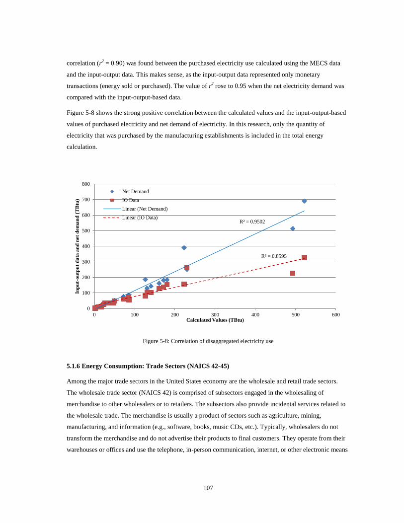
107
correlation (r2 = 0.90) was found between the purchased electricity use calculated using the MECS data
and the input-output data. This makes sense, as the input-output data represented only monetary
transactions (energy sold or purchased). The value of r2 rose to 0.95 when the net electricity demand was
compared with the input-output-based data.
Figure 5-8 shows the strong positive correlation between the calculated values and the input-output-based
values of purchased electricity and net demand of electricity. In this research, only the quantity of
electricity that was purchased by the manufacturing establishments is included in the total energy
calculation.
Figure 5-8: Correlation of disaggregated electricity use
5.1.6 Energy Consumption: Trade Sectors (NAICS 42-45)
Among the major trade sectors in the United States economy are the wholesale and retail trade sectors.
The wholesale trade sector (NAICS 42) is comprised of subsectors engaged in the wholesaling of
merchandise to other wholesalers or to retailers. The subsectors also provide incidental services related to
the wholesale trade. The merchandise is usually a product of sectors such as agriculture, mining,
manufacturing, and information (e.g., software, books, music CDs, etc.). Typically, wholesalers do not
transform the merchandise and do not advertise their products to final customers. They operate from their
warehouses or offices and use the telephone, in-person communication, internet, or other electronic means
R² = 0.9502
R² = 0.8595
0
100
200
300
400
500
600
700
800
0 100 200 300 400 500 600
Inp
ut-
ou
tpu
t d
ata
an
d n
et
dem
an
d (
TB
tu)
Calculated Values (TBtu)
Net Demand
IO Data
Linear (Net Demand)
Linear (IO Data)

108
to reach their customers. Two types of wholesalers operate in the United States economy. Wholesalers
selling merchandise on their account are merchant wholesalers. Establishments arranging the sales of
products within wholesalers and between wholesalers and retailers are business to business electronic
markets, brokers, agents, or commission merchants. Such establishments work for a fee or commission for
facilitating a product’s sale. Although wholesalers deal with sales of large volumes of capital and durable
goods to wholesalers and retailers, they also sell non-consumer capital and durable goods such as farm
equipment, industrial machinery, and vehicles used in the production and processing of goods and
services.
The Retail trade sector is made of subsectors that sell their merchandise to the final consumers such as
private households, institutional customers, and other commercial customers. They also provide incidental
and after sales services such as maintenance and repair. The sales of products occur in small quantities
from locations such as stores. Extensive advertising is used to promote their products and stores. Just like
wholesalers, retailers mostly do not transform their merchandise. However, in some cases such as optical
stores, the merchandise such as lenses may be grinded, cut, and transformed into another type of product
(e.g., prescription and sunglasses). There are two types of retailers: store retailers and non-store retailers.
The store retailers have a fixed point-of-sale location designed to handle a large crowd of customers. Such
stores use extensive amount of display and advertising in and out of stores. The non-stores include
retailers that are engaged in selling merchandise door-to-door and from portable stalls using electronic or
print catalogues, home demonstration, and direct response marketing (USCB, 2002c).
Among the major energy uses in the trade sectors are fuel use for heating and generating electrical power
and consumption of electricity in operating the business facilities such as warehouses, offices, stores, and
other related buildings. Fuel is also consumed by automobiles involved in trade activities. Energy use in
the wholesale and retail trade sectors was given in two categories: purchased fuel, and purchased
electricity. The cost of purchased fuel and electricity was reported in the business expenses report
published under the annual Economic Census by the United States Census Bureau. The fuel consumed by
motor vehicles was not included in the purchased fuel category.
Two main issues were found in the business expenses data. First, some energy data were missing because
the information was either unavailable or withheld due to poor data quality. In such cases, the known
quantities of fuel use given by the lower level NAICS codes were subtracted from those provided by the
higher level NAICS code. In some cases, where energy use for more than one subsector was missing, the
input-output data were used to disaggregate the fuel use of a higher level subsector and derive the energy
use for a lower level subsector. As mentioned earlier, the 2002 Benchmark Input-Output Accounts data
can be used to disaggregate the total energy use. However, as wholesale and retail trade establishments
may purchase energy to sell out to final consumers, using input-output data may be inaccurate. The 2002
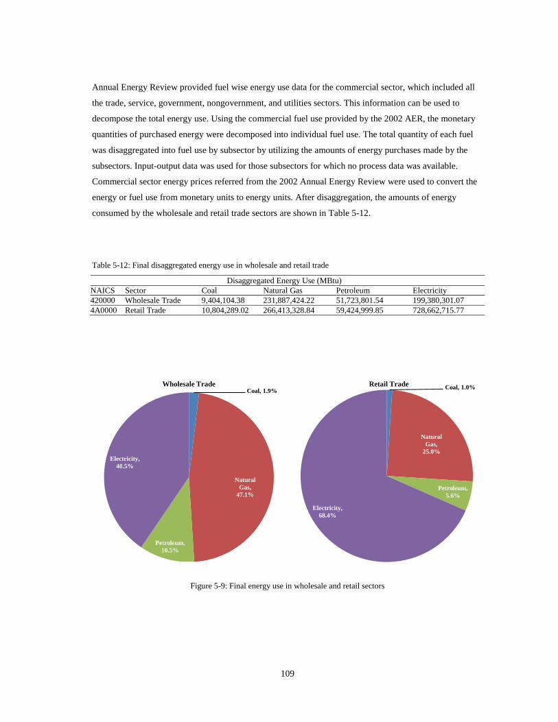
109
Annual Energy Review provided fuel wise energy use data for the commercial sector, which included all
the trade, service, government, nongovernment, and utilities sectors. This information can be used to
decompose the total energy use. Using the commercial fuel use provided by the 2002 AER, the monetary
quantities of purchased energy were decomposed into individual fuel use. The total quantity of each fuel
was disaggregated into fuel use by subsector by utilizing the amounts of energy purchases made by the
subsectors. Input-output data was used for those subsectors for which no process data was available.
Commercial sector energy prices referred from the 2002 Annual Energy Review were used to convert the
energy or fuel use from monetary units to energy units. After disaggregation, the amounts of energy
consumed by the wholesale and retail trade sectors are shown in Table 5-12.
Table 5-12: Final disaggregated energy use in wholesale and retail trade
Disaggregated Energy Use (MBtu)
NAICS Sector Coal Natural Gas Petroleum Electricity
420000 Wholesale Trade 9,404,104.38 231,887,424.22 51,723,801.54 199,380,301.07
4A0000 Retail Trade 10,804,289.02 266,413,328.84 59,424,999.85 728,662,715.77
Figure 5-9: Final energy use in wholesale and retail sectors
Coal, 1.9%
Natural
Gas,
47.1%
Petroleum,
10.5%
Electricity,
40.5%
Wholesale Trade Coal, 1.0%
Natural
Gas,
25.0%
Petroleum,
5.6%
Electricity,
68.4%
Retail Trade
110
Figure 5-9 provides a breakdown of fuel use by fuel type for the wholesale and retail sectors, respectively.
It is evident from the pie charts that use of natural gas and electricity dominates the wholesale and retail
sectors’ total energy use, respectively. As most retail trade establishments maintain large size stores and
use extensive use of electronic displays, dominance of electricity in total energy use seems reasonable.
5.1.7 Energy Consumption: Transportation and Warehousing Sectors (NAICS 48 & 49)
The transportation and warehousing sectors are made of subsectors involved in moving goods such as the
final products of manufacturing, mining, agriculture, information, and service sectors across cities and
states. These sectors also include scheduled and unscheduled human travel using rented vehicles such as
cars, buses, taxicabs, and trucks or through public transportation such as mass transit rail and road
systems. The transportation may be domestic or international. The subsectors are characterized by mode of
transportation such as land, water, and air. Railroad and road transportation are among the major surface
transportation modes. Airlines involved in passenger and cargo transportation are covered under air
transportation. Transporting goods and human labor using ships, barges, and boats are included in lake,
river, or deep seawater transportation. All travel activities for leisure, sightseeing, and recreational
purposes are included in scenic and sightseeing transportation (USCB, 2002c).
In addition, to move liquids and gases such as crude and refined petroleum and natural gas products, a
network of pipelines is used, which is categorized under pipeline transportation. Subsectors operating
warehouses and storage facilities for general merchandise, refrigerated products, and other products such
as equipment are represented by the warehousing and storage subsector. The warehousing and storage
subsectors may provide logistic services to distribute merchandise. They do not, however, sell any
product. All transportation subsectors require support activities such as vehicle maintenance and repair,
which are covered by a representing subsector. The movement of goods or information also involves
postal and courier services covered under subsectors: postal services, and courier and messenger services.
Table 5-13 lists the major subsectors that are engaged in transportation across geographic regions (USCB,
2002c).
Table 5-13: Major transportation sub-sectors (USCB, 2002c)
NAICS Sector and Subsector NAICS Sector and Subsector
481000 Air transportation 487000 Scenic and sightseeing transportation
482000 Rail transportation 488000 Support activities for transportation
483000 Water transportation 491000 Postal services
484000 Truck transportation 492000 Couriers and messengers
485000 Transit and ground passenger transportation 493000 Warehousing and storage
486000 Pipeline transportation
111
The United States’ transportation sector consumed over 27% (28.6 quadrillion Btu) of the nation’s total
energy in 2002. Among the major fuels consumed in transportation include gasoline, diesel, and jet fuel.
Other energy sources such as LPG, natural gas, residual fuel oil, and electricity were also used in
transportation activities. A significant amount of gasoline (95%) and diesel (68%) was used in highway
transportation and represented nearly 75% of the total transportation energy in 2002.
Figure 5-10 illustrates the dominance of gasoline and diesel (in monetary units) in highway, non-highway,
and off-highway transportation (in monetary units). Highway transportation included vehicles such as
motorcycles, cars, light trucks, buses, medium trucks, and heavy trucks or trailers. The non-highway mode
included all railroad, air, water, and pipeline transportation involving the use of pipelines and vehicles
such as trains, aircrafts, ships, barges, and boats. Fuel used by vehicles or moving equipment used in
personal and recreational activities (e.g., sports and leisure), and by the agriculture, construction, mining,
industrial, and commercial sectors was covered under the off-highway mode of transportation.
Figure 5-10 shows the breakdown of total transportation energy consumption by energy types (in energy
units). The transportation energy data were provided by the United States Department of Transportation
(USDOT) and Department of Energy by the mode of transportation (USDOT, 2012). A major issue with
these data was that no system was available for mapping the energy use by mode to energy use by NAICS
codes. Although subsectors such as air, rail, truck, and pipeline transportation were easy to map,
subsectors such as transit and ground passenger, scenic and sightseeing transportation, and support
activities for transportation were difficult to map due to overlapping activities. For instance, light vehicles
such as motorcycles, cars, and light trucks consumed a total of 16.2 quadrillion Btu of energy. These
vehicles included personal vehicles as well as taxicabs, limousines, emergency vehicles, and rented cars
and light trucks. All vehicles other than the personal ones needed to be mapped to the transit and ground
passenger transportation subsector. Similarly, the total energy consumed in air, water, and ground
transportation also included energy use in travel for sightseeing and scenic activities. This total energy was
also required to be decomposed into transportation energy for general and sightseeing purposes. Energy
use of support activities for transportation was not given in the transportation statistics provided by the
USDOT.
The fuel use data from the transportation statistics data were mapped directly to the input-output sectors of
air, rail, water, truck, and pipeline transportation. The passenger rail transportation was given by the
breakdown of transit, commuter, and intercity travel. The transit and commuter travel was allocated to
transit and ground passenger transportation. According to the 2002 vehicle fleet data from the National
Transportation Statistics (USDOT, 2012), nearly 31 and 4% of the total cars and light trucks, respectively
represented taxi or rental vehicles. Therefore, only 31 and 4% of the total fuel used by cars and light trucks
was counted in transit and ground passenger transportation. Other transportation components such as
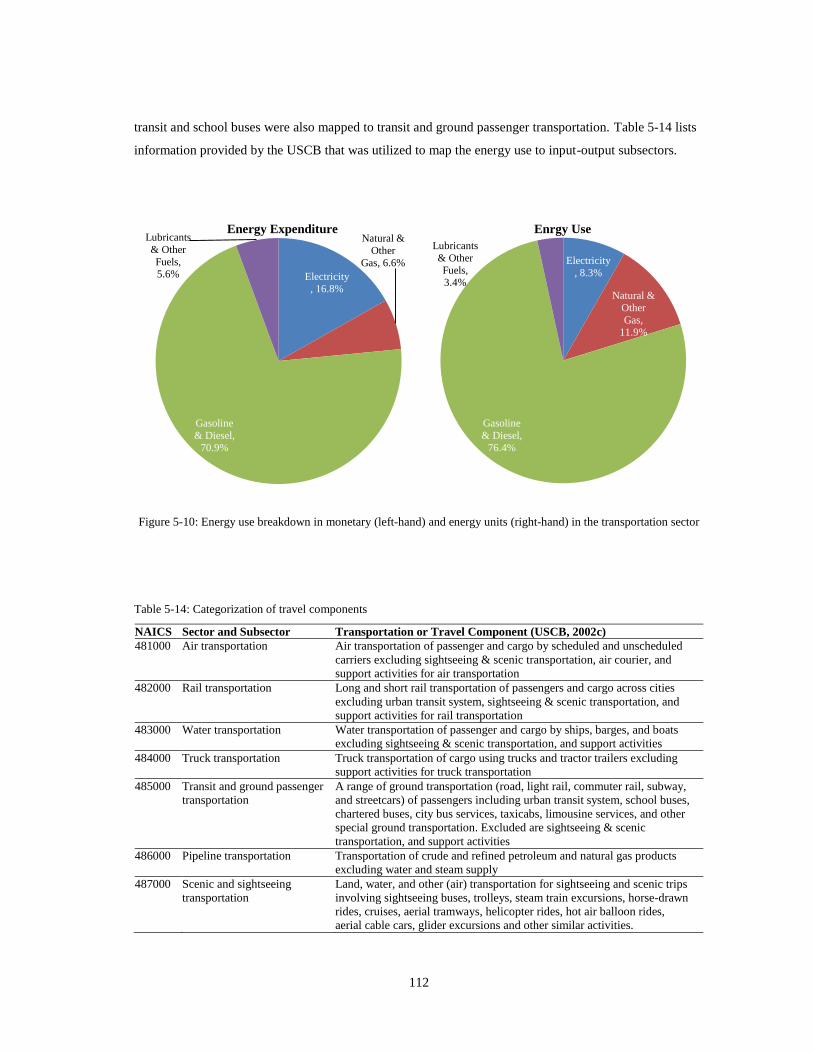
112
transit and school buses were also mapped to transit and ground passenger transportation. Table 5-14 lists
information provided by the USCB that was utilized to map the energy use to input-output subsectors.
Figure 5-10: Energy use breakdown in monetary (left-hand) and energy units (right-hand) in the transportation sector
Table 5-14: Categorization of travel components
NAICS Sector and Subsector Transportation or Travel Component (USCB, 2002c)
481000 Air transportation Air transportation of passenger and cargo by scheduled and unscheduled
carriers excluding sightseeing & scenic transportation, air courier, and
support activities for air transportation
482000 Rail transportation Long and short rail transportation of passengers and cargo across cities
excluding urban transit system, sightseeing & scenic transportation, and
support activities for rail transportation
483000 Water transportation Water transportation of passenger and cargo by ships, barges, and boats
excluding sightseeing & scenic transportation, and support activities
484000 Truck transportation Truck transportation of cargo using trucks and tractor trailers excluding
support activities for truck transportation
485000 Transit and ground passenger
transportation
A range of ground transportation (road, light rail, commuter rail, subway,
and streetcars) of passengers including urban transit system, school buses,
chartered buses, city bus services, taxicabs, limousine services, and other
special ground transportation. Excluded are sightseeing & scenic
transportation, and support activities
486000 Pipeline transportation Transportation of crude and refined petroleum and natural gas products
excluding water and steam supply
487000 Scenic and sightseeing
transportation
Land, water, and other (air) transportation for sightseeing and scenic trips
involving sightseeing buses, trolleys, steam train excursions, horse-drawn
rides, cruises, aerial tramways, helicopter rides, hot air balloon rides,
aerial cable cars, glider excursions and other similar activities.
Electricity
, 16.8%
Natural &
Other
Gas, 6.6%
Gasoline
& Diesel,
70.9%
Lubricants
& Other
Fuels, 5.6%
Energy Expenditure
Electricity
, 8.3%
Natural &
Other
Gas, 11.9%
Gasoline
& Diesel,
76.4%
Lubricants
& Other
Fuels, 3.4%
Enrgy Use
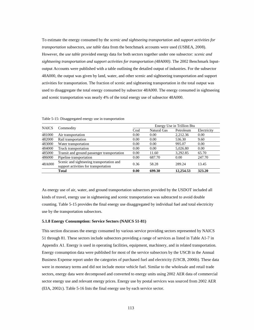
113
To estimate the energy consumed by the scenic and sightseeing transportation and support activities for
transportation subsectors, use table data from the benchmark accounts were used (USBEA, 2008).
However, the use table provided energy data for both sectors together under one subsector: scenic and
sightseeing transportation and support activities for transportation (48A000). The 2002 Benchmark Input-
output Accounts were published with a table outlining the detailed output of industries. For the subsector
48A000, the output was given by land, water, and other scenic and sightseeing transportation and support
activities for transportation. The fraction of scenic and sightseeing transportation in the total output was
used to disaggregate the total energy consumed by subsector 48A000. The energy consumed in sightseeing
and scenic transportation was nearly 4% of the total energy use of subsector 48A000.
Table 5-15: Disaggregated energy use in transportation
NAICS Commodity Energy Use in Trillion Btu
Coal Natural Gas Petroleum Electricity
481000 Air transportation 0.00 0.00 2,212.36 0.00
482000 Rail transportation 0.00 0.00 536.30 9.60
483000 Water transportation 0.00 0.00 995.07 0.00
484000 Truck transportation 0.00 0.00 5,026.80 0.00
485000 Transit and ground passenger transportation 0.00 11.60 3,292.85 65.70
486000 Pipeline transportation 0.00 687.70 0.00 247.70
48A000 Scenic and sightseeing transportation and
support activities for transportation 0.36 58.28 289.24 13.45
Total 0.00 699.30 12,254.53 323.20
As energy use of air, water, and ground transportation subsectors provided by the USDOT included all
kinds of travel, energy use in sightseeing and scenic transportation was subtracted to avoid double
counting. Table 5-15 provides the final energy use disaggregated by individual fuel and total electricity
use by the transportation subsectors.
5.1.8 Energy Consumption: Service Sectors (NAICS 51-81)
This section discusses the energy consumed by various service providing sectors represented by NAICS
51 through 81. These sectors include subsectors providing a range of services as listed in Table A1-7 in
Appendix A1. Energy is used in operating facilities, equipment, machinery, and in related transportation.
Energy consumption data were published for most of the service subsectors by the USCB in the Annual
Business Expense report under the categories of purchased fuel and electricity (USCB, 2006b). These data
were in monetary terms and did not include motor vehicle fuel. Similar to the wholesale and retail trade
sectors, energy data were decomposed and converted to energy units using 2002 AER data of commercial
sector energy use and relevant energy prices. Energy use by postal services was sourced from 2002 AER
(EIA, 2002c). Table 5-16 lists the final energy use by each service sector.
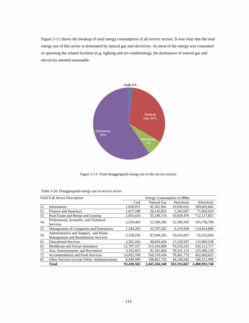
114
Figure 5-11 shows the breakup of total energy consumption of all service sectors. It was clear that the total
energy use of this sector is dominated by natural gas and electricity. As most of the energy was consumed
in operating the related facilities (e.g. lighting and air-conditioning), the dominance of natural gas and
electricity seemed reasonable.
Figure 5-11: Final disaggregated energy use in the service sectors
Table 5-16: Disaggregated energy use in service sector
NAICS & Sector Description Energy Consumption in MBtu
Coal Natural Gas Petroleum Electricity
51 Information 1,828,071 45,302,941 10,036,032 209,002,843
52 Finance and Insurance 1,017,188 28,145,852 5,342,697 71,962,024
53 Real Estate and Rental and Leasing 2,055,416 55,249,716 10,929,470 712,117,851
54 Professional, Scientific, and Technical
Services 2,254,402 55,589,280 12,399,503 105,758,789
55 Management of Companies and Enterprises 1,184,203 32,767,202 6,219,930 114,814,890
56 Administrative and Support, and Waste
Management and Remediation Services 3,530,250 87,049,292 19,416,837 55,555,936
61 Educational Services 3,282,204 90,819,420 17,239,507 132,900,538
62 Healthcare and Social Assistance 12,787,557 315,316,968 70,333,233 342,213,717
71 Arts, Entertainment, and Recreation 3,332,853 82,181,844 18,331,125 125,386,129
72 Accommodation and Food Services 14,452,708 356,376,434 79,491,779 452,669,023
81 Other Services (except Public Administration) 8,049,990 198,861,742 44,246,045 166,521,999
Total 93,438,582 2,445,166,340 502,316,667 2,488,903,740
Coal, 1%
Natural
Gas, 32%
Petroleum,
7%
Electricity,
59%
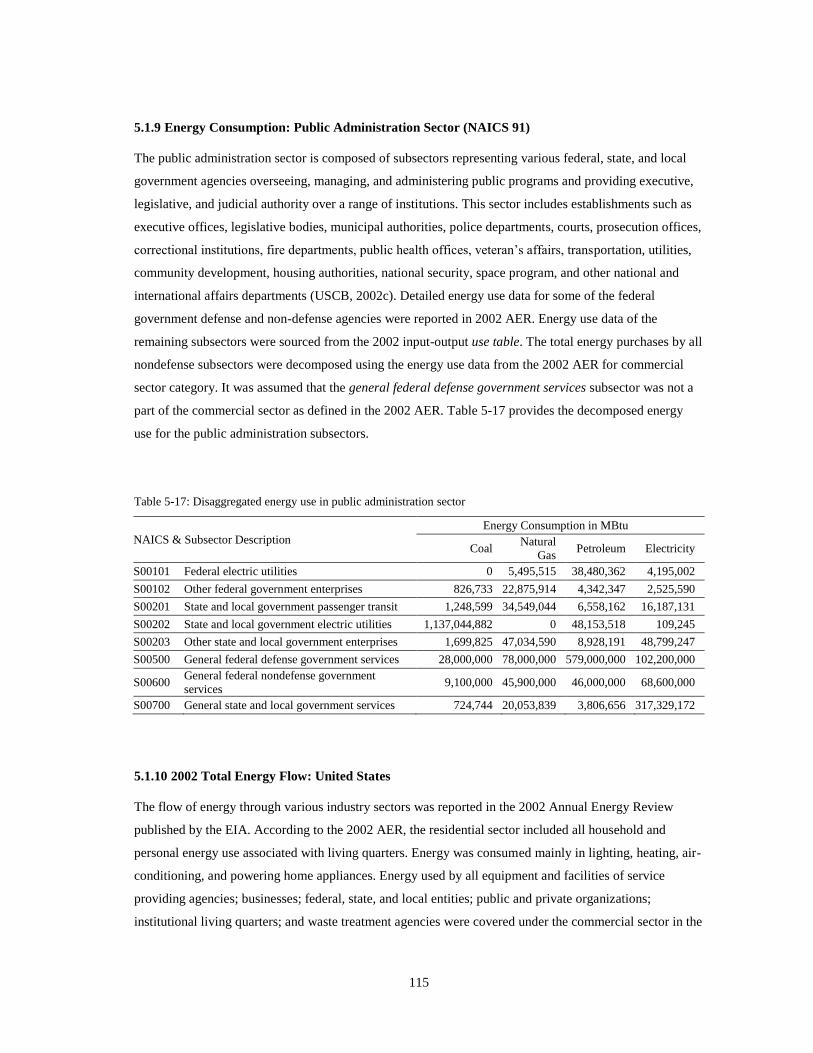
115
5.1.9 Energy Consumption: Public Administration Sector (NAICS 91)
The public administration sector is composed of subsectors representing various federal, state, and local
government agencies overseeing, managing, and administering public programs and providing executive,
legislative, and judicial authority over a range of institutions. This sector includes establishments such as
executive offices, legislative bodies, municipal authorities, police departments, courts, prosecution offices,
correctional institutions, fire departments, public health offices, veteran’s affairs, transportation, utilities,
community development, housing authorities, national security, space program, and other national and
international affairs departments (USCB, 2002c). Detailed energy use data for some of the federal
government defense and non-defense agencies were reported in 2002 AER. Energy use data of the
remaining subsectors were sourced from the 2002 input-output use table. The total energy purchases by all
nondefense subsectors were decomposed using the energy use data from the 2002 AER for commercial
sector category. It was assumed that the general federal defense government services subsector was not a
part of the commercial sector as defined in the 2002 AER. Table 5-17 provides the decomposed energy
use for the public administration subsectors.
Table 5-17: Disaggregated energy use in public administration sector
NAICS & Subsector Description
Energy Consumption in MBtu
Coal Natural
Gas Petroleum Electricity
S00101 Federal electric utilities 0 5,495,515 38,480,362 4,195,002
S00102 Other federal government enterprises 826,733 22,875,914 4,342,347 2,525,590
S00201 State and local government passenger transit 1,248,599 34,549,044 6,558,162 16,187,131
S00202 State and local government electric utilities 1,137,044,882 0 48,153,518 109,245
S00203 Other state and local government enterprises 1,699,825 47,034,590 8,928,191 48,799,247
S00500 General federal defense government services 28,000,000 78,000,000 579,000,000 102,200,000
S00600 General federal nondefense government
services 9,100,000 45,900,000 46,000,000 68,600,000
S00700 General state and local government services 724,744 20,053,839 3,806,656 317,329,172
5.1.10 2002 Total Energy Flow: United States
The flow of energy through various industry sectors was reported in the 2002 Annual Energy Review
published by the EIA. According to the 2002 AER, the residential sector included all household and
personal energy use associated with living quarters. Energy was consumed mainly in lighting, heating, air-
conditioning, and powering home appliances. Energy used by all equipment and facilities of service
providing agencies; businesses; federal, state, and local entities; public and private organizations;
institutional living quarters; and waste treatment agencies were covered under the commercial sector in the
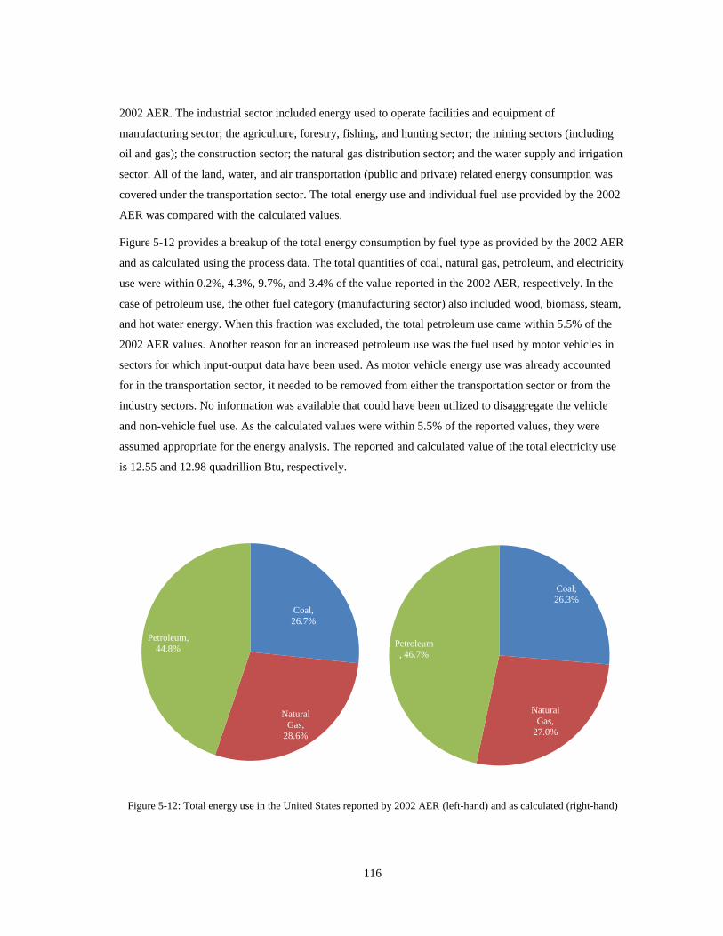
116
2002 AER. The industrial sector included energy used to operate facilities and equipment of
manufacturing sector; the agriculture, forestry, fishing, and hunting sector; the mining sectors (including
oil and gas); the construction sector; the natural gas distribution sector; and the water supply and irrigation
sector. All of the land, water, and air transportation (public and private) related energy consumption was
covered under the transportation sector. The total energy use and individual fuel use provided by the 2002
AER was compared with the calculated values.
Figure 5-12 provides a breakup of the total energy consumption by fuel type as provided by the 2002 AER
and as calculated using the process data. The total quantities of coal, natural gas, petroleum, and electricity
use were within 0.2%, 4.3%, 9.7%, and 3.4% of the value reported in the 2002 AER, respectively. In the
case of petroleum use, the other fuel category (manufacturing sector) also included wood, biomass, steam,
and hot water energy. When this fraction was excluded, the total petroleum use came within 5.5% of the
2002 AER values. Another reason for an increased petroleum use was the fuel used by motor vehicles in
sectors for which input-output data have been used. As motor vehicle energy use was already accounted
for in the transportation sector, it needed to be removed from either the transportation sector or from the
industry sectors. No information was available that could have been utilized to disaggregate the vehicle
and non-vehicle fuel use. As the calculated values were within 5.5% of the reported values, they were
assumed appropriate for the energy analysis. The reported and calculated value of the total electricity use
is 12.55 and 12.98 quadrillion Btu, respectively.
Figure 5-12: Total energy use in the United States reported by 2002 AER (left-hand) and as calculated (right-hand)
Coal,
26.7%
Natural
Gas,
28.6%
Petroleum,
44.8%
Coal,
26.3%
Natural
Gas,
27.0%
Petroleum
, 46.7%

117
5.2 SUMMARY
The process data of energy used by energy sources were collected for nearly all industry sectors. Some
data such as electricity use were given in energy units (kWh), whereas some data were provided in
monetary units. Appropriate energy prices were used to convert the energy use from monetary data to
energy units. Three primary fuels, namely coal, natural gas, petroleum dominated the total energy supply
in the United States in 2002. According to the calculations of this study, nearly 22.8, 23.4, and 40.4
quadrillion Btu of coal, natural gas, and petroleum was consumed in the United States, respectively. The
total fossil fuel based energy supply was calculated as 86.6 quadrillion Btu, which was within 1% of the
value reported by the 2002 Annual Energy Review. The total consumption of electricity was calculated as
12.98 quadrillion Btu, which was within 3% of the 2002 Annual Energy Review. The energy used by each
industry sector was calculated by energy source. Since some industry sectors purchased energy directly
from the oil and gas sector, a separate energy row of such purchases was estimated.
The energy use data was available for more than half of the industry sectors in physical units. However, in
the case of some industry sectors such as service industries, the data was in monetary units. Although, the
monetary data was used only to proportionately allocate the total energy use, availability of detailed
energy use data in energy units would have been better. In the future, one can expect an availability of
detailed energy use data by each energy source for the service sectors.
118
CHAPTER VI
PRIMARY ENERGY FACTOR CALCULATION
6.
6.1 PRIMARY AND SECONDARY ENERGY
The energy consumed by various economic sectors is either in a primary or a secondary energy form
(Deru and Torcellini, 2007; Dixit et al., 2010). The primary energy is the energy of a fuel extracted
directly from earth. Fossil fuels such as coal, crude oil, and gas are extracted directly from the earth and
are known as primary fuels. The secondary energy (also known as delivered energy) is the energy that is
generated by processing the primary fuels. For instance, gasoline that is processed and refined from crude
oil is a secondary or delivered fuel, whereas the crude oil is a primary fuel. Another example of secondary
energy is electricity, which is generated mostly by combusting primary fuels such as coal, petroleum, and
natural gas. The primary and secondary energies are also known as source and site energy, respectively. It
is important to distinguish primary energy from secondary energy, as the two are not comparable and
represent different amounts of energy. For example, it will be inaccurate to compare the energy use of two
buildings if one is expressed in a primary (source energy e.g. in Btu) and the other in a secondary energy
term (e.g. electricity in kWh). The amount of electricity use could be significantly higher when converted
to a primary energy term. It is due to the energy conversion and transmission and distribution (T&D)
losses that incur while producing and distributing the electricity. The process of generating electricity
could use 2 - 3 times more coal, oil, or natural gas in generating one unit of electricity. Similarly, the
process of producing and distributing other secondary fuels such as consumer grade natural gas and
gasoline also involves energy use and energy losses (or gains), which should also be accounted for when
converting them to primary energy terms. All secondary energy use quantities should be converted to a
primary or source energy term before a comparison is made.
6.2 PRIMARY ENERGY FACTOR (PEF)
In this research, the term primary energy means the sum of energy consumed by an economic sector and
the energy that is required to extract, process, convert, transmit, and distribute the consumed energy. Both,
the primary and secondary energy sources have consumed a significant amount of energy before they
reach to the end users. In the process of their extraction and delivery, primary fuels such as coal also
consume a considerable amount of energy. The ratio of the total amount of energy delivered to the end
users to the total amount of energy consumed (including the delivered energy) in delivering that energy is
termed the Primary Energy Factor (PEF). A PEF represents the total primary energy needed to produce a
unit of energy delivered for end use. Hence:
119
Equation 6-1
The above expression should be adjusted for the energy losses that incur during extraction, processing, and
delivery of an energy source. The numerator in the above equation denotes the delivered energy, for
instance, electricity or consumer grade natural gas. The denominator represents the total primary energy
used and lost in the process of delivery (including the energy spent in extraction, processing, conversion,
and distribution). This total primary energy used in the process of delivering the energy for end use is
made of one or more of the three major components as shown in Figure 6-1. The following sections
describe these components:
6.2.1 Primary Fuel Use
At this stage, a primary fuel is either burnt (e.g. in power plants) or used as a raw material (e.g. in oil
refineries) to be processed or refined further. The total energy consumed at this stage has a direct and an
indirect component. The direct fraction includes combustion energy, whereas the indirect energy fraction
consists of pre-combustion energy.
Combustion Energy: The combustion energy represents the calorific value of a fuel or energy source that
is released when the fuel is burnt. The process of fossil fuel combustion is a chemical reaction involving
oxygen that results in release of water, CO2, and heat. The amount of heat energy produced in the fuel
combustion process represents the combustion energy of a fuel (see Figure 6-1).
Pre-combustion Energy: The pre-combustion energy is the energy consumed in extracting, processing,
converting, and distributing a fossil fuel that is being combusted, processed, or refined. This fraction of
energy covers all fuel and nonfuel inputs. The use of primary fuel as an energy input and as a feedstock
material is included under the fuel input category. The nonfuel inputs cover the energy embodied in raw
materials, equipment, and labor that are used in processing, refining, and delivering the energy for end use.
6.2.2 Energy Use in Plant or Lease Operation and Energy Delivery
The plants such as natural gas processing facilities, petroleum refineries, and power plants consume
energy in their operations. Energy is also used when energy source or fuel is distributed to end users.
Similarly, operations of oil and gas wells, coal and uranium mines, and related facilities also use a
significant amount of energy. Such operations also need built structures, equipment, and raw materials,
which also have consumed energy when they were manufactured or installed.
Direct Energy: The primary and secondary energy used by plants, lease operations, or mine facilities and
equipment in their operations is accounted for in this fraction. The energy consumed in distributing the

120
processed fuel is also added to the total operating energy. The energy of labor is also included (see Figure
6-1).
Indirect Fraction of Operating Energy: The amount of energy that is consumed in extracting, processing,
converting, and distributing the operating energy is included in this fraction. In addition, the energy
embodied in built facilities, materials, equipment, and labor is also accounted for (see Figure 6-1).
Figure 6-1: Energy components used in delivering energy for end use
6.2.3 Energy Lost and Gained
In the process of energy extraction, processing, refining, conversion, and distribution, a significant amount
of energy is either lost or gained (in the case of petroleum refineries). Just like any other primary energy,
this fraction of energy also has a direct and an indirect component.
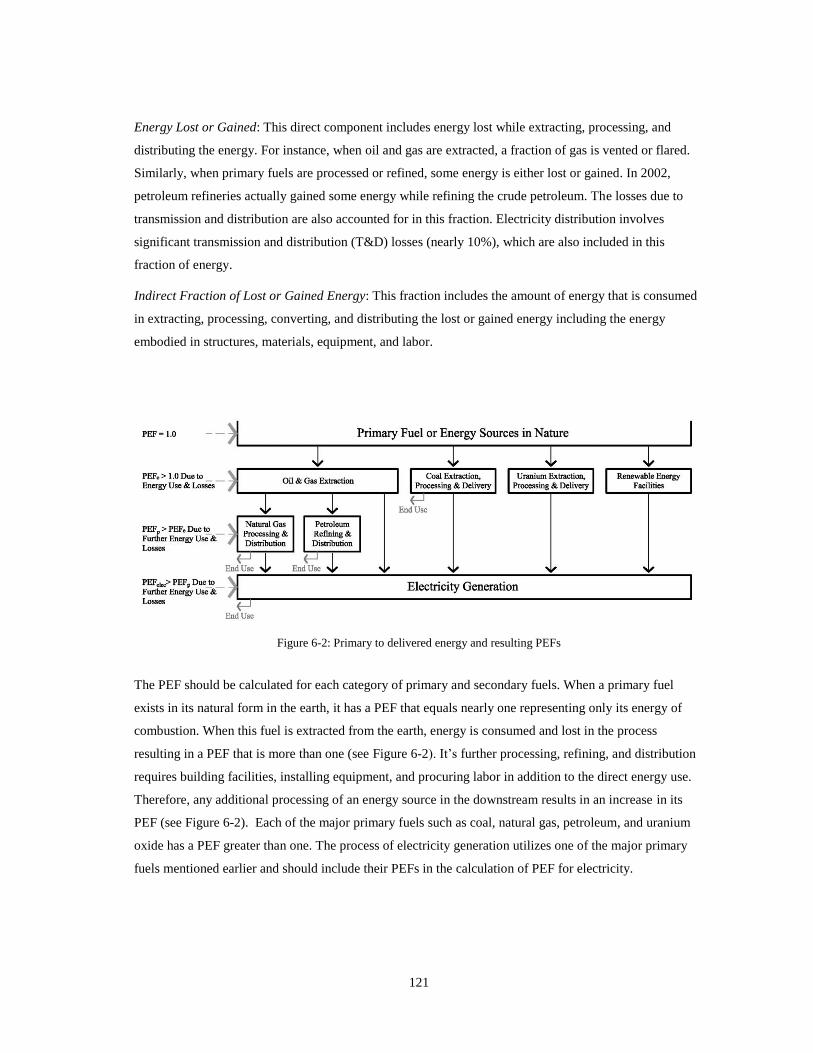
121
Energy Lost or Gained: This direct component includes energy lost while extracting, processing, and
distributing the energy. For instance, when oil and gas are extracted, a fraction of gas is vented or flared.
Similarly, when primary fuels are processed or refined, some energy is either lost or gained. In 2002,
petroleum refineries actually gained some energy while refining the crude petroleum. The losses due to
transmission and distribution are also accounted for in this fraction. Electricity distribution involves
significant transmission and distribution (T&D) losses (nearly 10%), which are also included in this
fraction of energy.
Indirect Fraction of Lost or Gained Energy: This fraction includes the amount of energy that is consumed
in extracting, processing, converting, and distributing the lost or gained energy including the energy
embodied in structures, materials, equipment, and labor.
Figure 6-2: Primary to delivered energy and resulting PEFs
The PEF should be calculated for each category of primary and secondary fuels. When a primary fuel
exists in its natural form in the earth, it has a PEF that equals nearly one representing only its energy of
combustion. When this fuel is extracted from the earth, energy is consumed and lost in the process
resulting in a PEF that is more than one (see Figure 6-2). It’s further processing, refining, and distribution
requires building facilities, installing equipment, and procuring labor in addition to the direct energy use.
Therefore, any additional processing of an energy source in the downstream results in an increase in its
PEF (see Figure 6-2). Each of the major primary fuels such as coal, natural gas, petroleum, and uranium
oxide has a PEF greater than one. The process of electricity generation utilizes one of the major primary
fuels mentioned earlier and should include their PEFs in the calculation of PEF for electricity.
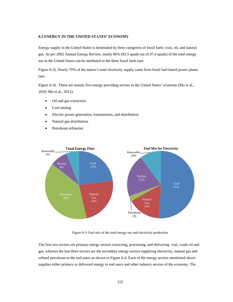
122
6.3 ENERGY IN THE UNITED STATES’ ECONOMY
Energy supply in the United States is dominated by three categories of fossil fuels: coal, oil, and natural
gas. As per 2002 Annual Energy Review, nearly 86% (83.5 quads out of 97.4 quads) of the total energy
use in the United States can be attributed to the three fossil fuels (see
Figure 6-3). Nearly 70% of the nation’s total electricity supply came from fossil fuel-based power plants
(see
Figure 6-3). There are mainly five energy providing sectors in the United States’ economy (Mo et al.,
2010; Mo et al., 2011):
Oil and gas extraction
Coal mining
Electric power generation, transmission, and distribution
Natural gas distribution
Petroleum refineries
Figure 6-3: Fuel mix of the total energy use and electricity production
The first two sectors are primary energy sectors extracting, processing, and delivering coal, crude oil and
gas, whereas the last three sectors are the secondary energy sectors supplying electricity, natural gas and
refined petroleum to the end users as shown in Figure 6-4. Each of the energy sectors mentioned above
supplies either primary or delivered energy to end users and other industry sectors of the economy. The
Coal
23%
Natural
Gas
24%
Petroleum
39%
Nuclear
8%
Renewable
6%
Total Energy Flow
Coal
51%
Natural
Gas
16%
Petroleum
2%
Nuclear
21%
Renewable
10%
Fuel Mix for Electricity
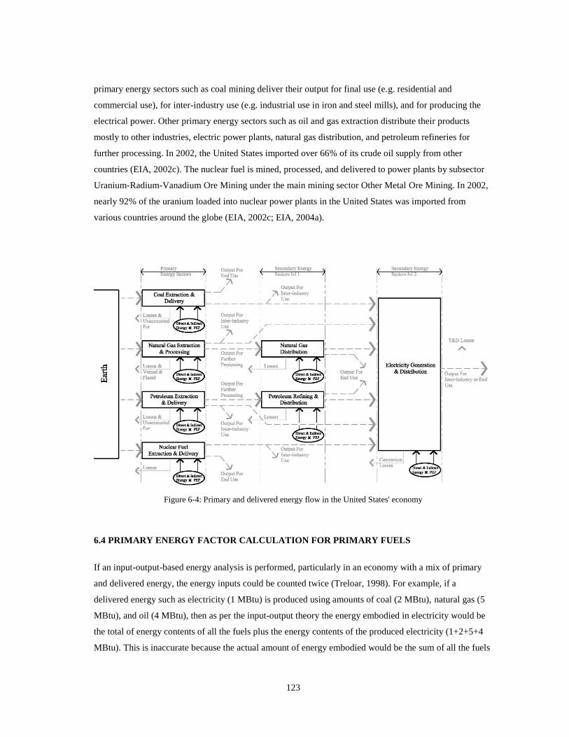
123
primary energy sectors such as coal mining deliver their output for final use (e.g. residential and
commercial use), for inter-industry use (e.g. industrial use in iron and steel mills), and for producing the
electrical power. Other primary energy sectors such as oil and gas extraction distribute their products
mostly to other industries, electric power plants, natural gas distribution, and petroleum refineries for
further processing. In 2002, the United States imported over 66% of its crude oil supply from other
countries (EIA, 2002c). The nuclear fuel is mined, processed, and delivered to power plants by subsector
Uranium-Radium-Vanadium Ore Mining under the main mining sector Other Metal Ore Mining. In 2002,
nearly 92% of the uranium loaded into nuclear power plants in the United States was imported from
various countries around the globe (EIA, 2002c; EIA, 2004a).
Figure 6-4: Primary and delivered energy flow in the United States' economy
6.4 PRIMARY ENERGY FACTOR CALCULATION FOR PRIMARY FUELS
If an input-output-based energy analysis is performed, particularly in an economy with a mix of primary
and delivered energy, the energy inputs could be counted twice (Treloar, 1998). For example, if a
delivered energy such as electricity (1 MBtu) is produced using amounts of coal (2 MBtu), natural gas (5
MBtu), and oil (4 MBtu), then as per the input-output theory the energy embodied in electricity would be
the total of energy contents of all the fuels plus the energy contents of the produced electricity (1+2+5+4
MBtu). This is inaccurate because the actual amount of energy embodied would be the sum of all the fuels
124
(11 MBtu) that were consumed. One must be careful to do some adjustments to avoid double counting
before using the input-output framework (Treloar, 1998). In addition, it is important to note that the
indirect fraction of energy due to all energy and nonenergy inputs should not remain excluded from the
calculation.
In this research, the PEFs for all major fuels were calculated using three approaches. In the first approach,
the direct energy fraction was calculated on the basis of process data of energy use and losses. The indirect
energy fraction was calculated and added using the input-output framework. The direct requirements were
subtracted from the total requirements to estimate the indirect energy fraction. The direct energy process
data and indirect energy input-output data were then totaled and adjusted for the energy losses. The PEFs
for fuels such as coal, natural gas, petroleum, and nuclear fuel were calculated first. The PEF for
electricity was then computed using the direct energy data and the calculated values of PEFs for the four
fuels. There was no need to use the input-output data for electricity, as the PEFs represented the indirect
impacts of its production. Both the human and capital energy inputs were included in the calculation. The
following sections describe the first approach in detail, as the results of this approach were adopted in this
research.
It is assumed that nearly all of the natural gas supplied to the end users was distributed through the natural
gas distribution sector. Additionally, all refined petroleum products were assumed to come from the
petroleum refineries sector. It is important to calculate the PEFs separately for oil and gas extraction,
natural gas distribution, and petroleum refineries sectors, as some industry sectors made purchases directly
from all three sectors. Hence, a set of PEFs representing each energy providing sector must be derived for
those purchases. The PEFs of the coal mining, oil and gas extraction, natural gas distribution, petroleum
refineries, and the uranium-radium-vanadium ore mining were used to compute the PEF of electricity
production.
6.4.1 Oil and Gas Extraction
The fuel and electricity consumption data were sourced from the 2002 Economic Census (USCB, 2004)
for the two sectors involved in oil and gas extraction. The sectors were:
Crude petroleum and natural gas extraction
Natural gas liquid extraction
This sector drew crude oil and natural gas from the earth and processed the natural gas into a dry and
consumable form in order to distribute it for the end use. In the natural gas processing plants, dry
consumer-grade natural gas was produced. To produce dry natural gas, the liquefiable hydrocarbons and
non-hydrocarbon gases (e.g., water vapor, carbon dioxide (CO2), helium, hydrogen sulfide and nitrogen)
were removed from the extracted volume of natural gas (EIA, 2004b; NPC, 2011). There were only two
components of total primary energy use in these sectors. First, the energy used in lease and plant
125
operations and second, the energy lost while extracting and processing the oil and gas. The fuel
consumption data were provided in energy and monetary terms. In the case of missing data in energy
terms, appropriate energy prices were used to convert the monetary data to energy terms.
Total direct energy use (Ed, og) is the sum of the energies of all types of fuels consumed in the operations of
oil and gas extraction facilities. The total energy consumed in processing and distributing dry natural gas
included both the direct (Ed, og) and indirect fraction (Ein, og). The consumption of fuel from the energy
providing sectors caused the other industry sectors to increase their production to meet the demand. This
increase in production represented the indirect requirements. The 2002 Benchmark Input-output Accounts
were referred (USBEA, 2008) and direct requirement coefficients are subtracted from the total
requirement coefficients for estimating the indirect energy requirements (Ein, og) of the oil and gas
extraction sector. The indirect requirements were in monetary units, and hence, converted to energy units
by using energy prices. There are two options for using energy prices: the annual average wellhead price
($2.95/1000 CF) for natural gas and domestic first purchase price ($24.65/bbl.) for crude oil. According to
the 2002 Annual Energy Review (EIA, 2002c), the wellhead price included all costs before shipping the
natural gas from the lease. In addition, a United States average for consumer grade natural gas and refined
petroleum could be derived and used. However, this was difficult, particularly in the case of refined
petroleum that included multiple products with varying prices and varying levels of uses. Another option
was to derive an average energy price as a ratio of the total monetary output to the total energy output of
the energy providing sector. Such a price was assumed to be a better representative of the national energy
economy.
Table 6-1 lists major energy parameters used for calculating the PEF for major energy sources. Human
energy and the energy embodied in capital inputs is then added to the calculated direct and indirect energy
values for coal, natural gas, petroleum, and electricity. The extraction of natural gas and oil also incurs
production and processing losses. The production losses include the volume of natural gas that is vented
and flared during the extraction process. The processing results in extraction losses. The extraction loss
data were sourced from (EIA, 2002c; EIA, 2004b). The total amount of natural gas leakage was sourced
from the California Air Resources Board report (ARB, 2009). The sum of all extraction and processing
losses is termed total oil and gas loss (Log).
If the combustion and pre-combustion energy factors are represented by EFC, og and EFP, og, respectively,
then:
Equation 6-2
∑
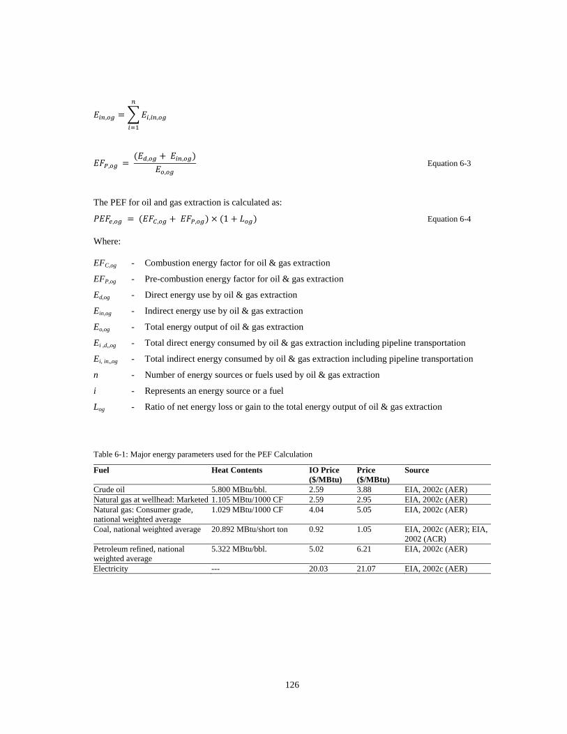
126
∑
Equation 6-3
The PEF for oil and gas extraction is calculated as:
Equation 6-4
Where:
EFC,og - Combustion energy factor for oil & gas extraction
EFP,og - Pre-combustion energy factor for oil & gas extraction
Ed,og - Direct energy use by oil & gas extraction
Ein,og - Indirect energy use by oil & gas extraction
Eo,og - Total energy output of oil & gas extraction
Ei ,d,,og - Total direct energy consumed by oil & gas extraction including pipeline transportation
Ei, in,,og - Total indirect energy consumed by oil & gas extraction including pipeline transportation
n - Number of energy sources or fuels used by oil & gas extraction
i - Represents an energy source or a fuel
Log - Ratio of net energy loss or gain to the total energy output of oil & gas extraction
Table 6-1: Major energy parameters used for the PEF Calculation
Fuel Heat Contents IO Price
($/MBtu)
Price
($/MBtu)
Source
Crude oil 5.800 MBtu/bbl. 2.59 3.88 EIA, 2002c (AER)
Natural gas at wellhead: Marketed 1.105 MBtu/1000 CF 2.59 2.95 EIA, 2002c (AER)
Natural gas: Consumer grade,
national weighted average
1.029 MBtu/1000 CF 4.04 5.05 EIA, 2002c (AER)
Coal, national weighted average 20.892 MBtu/short ton 0.92 1.05 EIA, 2002c (AER); EIA,
2002 (ACR)
Petroleum refined, national
weighted average
5.322 MBtu/bbl. 5.02 6.21 EIA, 2002c (AER)
Electricity --- 20.03 21.07 EIA, 2002c (AER)
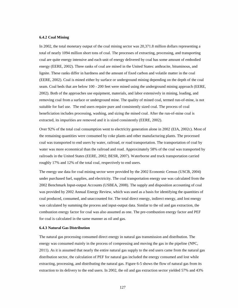
127
6.4.2 Coal Mining
In 2002, the total monetary output of the coal mining sector was 20,371.8 million dollars representing a
total of nearly 1094 million short tons of coal. The processes of extracting, processing, and transporting
coal are quite energy intensive and each unit of energy delivered by coal has some amount of embodied
energy (EERE, 2002). Three ranks of coal are mined in the United States: anthracite, bituminous, and
lignite. These ranks differ in hardness and the amount of fixed carbon and volatile matter in the coal
(EERE, 2002). Coal is mined either by surface or underground mining depending on the depth of the coal
seam. Coal beds that are below 100 - 200 feet were mined using the underground mining approach (EERE,
2002). Both of the approaches use equipment, materials, and labor extensively in mining, loading, and
removing coal from a surface or underground mine. The quality of mined coal, termed run-of-mine, is not
suitable for fuel use. The end users require pure and consistently sized coal. The process of coal
beneficiation includes processing, washing, and sizing the mined coal. After the run-of-mine coal is
extracted, its impurities are removed and it is sized consistently (EERE, 2002).
Over 92% of the total coal consumption went to electricity generation alone in 2002 (EIA, 2002c). Most of
the remaining quantities were consumed by coke plants and other manufacturing plants. The processed
coal was transported to end users by water, railroad, or road transportation. The transportation of coal by
water was more economical than the railroad and road. Approximately 58% of the coal was transported by
railroads in the United States (EERE, 2002; BESR, 2007). Waterborne and truck transportation carried
roughly 17% and 12% of the total coal, respectively to end users.
The energy use data for coal mining sector were provided by the 2002 Economic Census (USCB, 2004)
under purchased fuel, supplies, and electricity. The coal transportation energy use was calculated from the
2002 Benchmark Input-output Accounts (USBEA, 2008). The supply and disposition accounting of coal
was provided by 2002 Annual Energy Review, which was used as a basis for identifying the quantities of
coal produced, consumed, and unaccounted for. The total direct energy, indirect energy, and lost energy
was calculated by summing the process and input-output data. Similar to the oil and gas extraction, the
combustion energy factor for coal was also assumed as one. The pre-combustion energy factor and PEF
for coal is calculated in the same manner as oil and gas.
6.4.3 Natural Gas Distribution
The natural gas processing consumed direct energy in natural gas transmission and distribution. The
energy was consumed mainly in the process of compressing and moving the gas in the pipeline (NPC,
2011). As it is assumed that nearly the entire natural gas supply to the end users came from the natural gas
distribution sector, the calculation of PEF for natural gas included the energy consumed and lost while
extracting, processing, and distributing the natural gas. Figure 6-5 shows the flow of natural gas from its
extraction to its delivery to the end users. In 2002, the oil and gas extraction sector yielded 57% and 43%
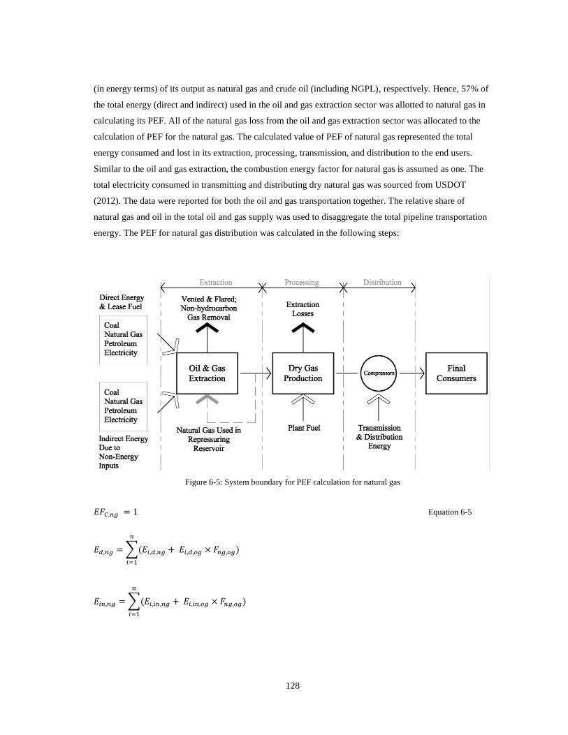
128
(in energy terms) of its output as natural gas and crude oil (including NGPL), respectively. Hence, 57% of
the total energy (direct and indirect) used in the oil and gas extraction sector was allotted to natural gas in
calculating its PEF. All of the natural gas loss from the oil and gas extraction sector was allocated to the
calculation of PEF for the natural gas. The calculated value of PEF of natural gas represented the total
energy consumed and lost in its extraction, processing, transmission, and distribution to the end users.
Similar to the oil and gas extraction, the combustion energy factor for natural gas is assumed as one. The
total electricity consumed in transmitting and distributing dry natural gas was sourced from USDOT
(2012). The data were reported for both the oil and gas transportation together. The relative share of
natural gas and oil in the total oil and gas supply was used to disaggregate the total pipeline transportation
energy. The PEF for natural gas distribution was calculated in the following steps:
Figure 6-5: System boundary for PEF calculation for natural gas
Equation 6-5
∑
∑
129
Equation 6-6
The PEF for natural gas is estimated as:
Equation 6-7
Where:
EFC,ng - Combustion energy factor for natural gas
EFP,ng - Pre-combustion energy factor for natural gas
Ed,ng - Direct energy use by natural gas
Ein,ng - Indirect energy use by natural gas
Eo,ng - Total energy output of natural gas
Ei ,d,,ng - Total direct energy consumed by natural gas including pipeline transportation
Ei ,d,,og - Total direct energy consumed by oil & gas extraction sector
Ei, in,,ng - Total indirect energy consumed by natural gas including pipeline transportation
Ei ,in,,og - Total indirect energy consumed by oil & gas extraction sector
Fng,og - Natural gas as a fraction of total energy output of oil and gas extraction sector
n - Number of energy sources or fuels used by natural gas
i - Represents an energy source or a fuel
Lng - Ratio of net energy loss or gain to the total energy output of natural gas
6.4.4 Petroleum Refineries
In 2002, the United States produced and imported 5.82 and 9.05 million bbl. of crude oil every day,
respectively. Petroleum refineries used crude oil and produced a range of fuel and chemical products such
as gasoline, kerosene, and naphtha. Petroleum refining is a complex process that involves separating,
cracking, restructuring, treating, and mixing hydrocarbons to produce the refined products. These
processes consume energy and also result in energy losses or gains. In 2002, the refining of petroleum
resulted in 0.117 million bbl. of unaccounted crude oil. In addition, a total of 349.15 million bbl. of
petroleum was reported as an energy gain. Similar to the natural gas sector, it was assumed that all of the
petroleum products supplied to the national economy came only from the petroleum refineries sector. It
means that all of the upstream energy use should also be taken into account in the PEF calculation. As
nearly 43% of the oil and gas sector output consisted of crude oil, 43% of the energy use was allocated to
petroleum products and added to the total direct and indirect energy use. The PEF was calculated in the
same steps as the natural gas distribution.

130
6.4.5 Nuclear Fuel
In 2002, nearly 52.7 million pounds of uranium oxide was imported against 2.34 million pounds of
domestic production. The total uranium purchases made by electric power plants from domestic suppliers
in the United States totaled 22.7 million pounds. A total of 57.3 million pounds of uranium was loaded
into the nuclear power reactors as a fuel in 2002 (EIA, 2004b). The uranium-radium-vanadium ore mining,
a subsector of the gold, silver, and other metal ore mining sector, extracts the uranium used by the nuclear
power plants. The total amount of uranium extracted, processed and consumed domestically for generating
electricity can be used to disaggregate the sector to calculate the indirect energy use for nuclear fuel. It is
assumed that the imported quantities of nuclear fuel were extracted, processed, and delivered domestically.
Process data of energy required to extract, process, and deliver 1000 pounds of uranium were used to
calculate the direct energy use. These data were sourced from the Oregon Department of Environmental
Quality report (ODEQ, 2004). The indirect energy fraction was calculated using the input-output approach
similar to other primary fuels. The energy contents of uranium were calculated using the amount of total
nuclear energy consumed and the total quantity of uranium consumed in nuclear power plants in 2002.
6.4.6 Electricity
Electricity is produced in electric power plants using a range of nonrenewable fuels such as coal, natural
gas, oil, and nuclear fuel. Most of the fossil fuel-based power plants burn fossil fuels for producing steam
to run the turbines. In nuclear power plants, the fission process of nuclear fuel in nuclear reactors is used
to generate steam. Renewable energy sources such as wind, solar energy, hydropower, biomass,
geothermal, and tidal energy are also utilized to generate electrical power. The fuel mix used for
generating the electricity differs in different regions depending on the availability of energy sources. The
production of one unit of electricity from fossil fuel combustion usually requires 2 - 3 times more energy
due to lower energy conversion efficiency. The combustion energy factor, which is assumed as one for
primary fuel is more than one in the case of electricity production.
Approximately 50% of the electricity generated in the United States came from fossil fuel-based power
plants in 2002. Figure B1-16 in Appendix B1 illustrates the trends in the use of energy sources for
producing electrical power in the United States from 1949 through 2011. Fossil fuels clearly dominated
the electricity generation sector in the country. Furthermore, a detailed look at the fossil fuel use for
electricity production revealed the clear dominance of coal from 1949 - 2011(see Figure B1-17 in
Appendix B1). In 2002, over 50% of electricity was produced using coal alone. Nearly 70% of the total
United States’ electricity generation was attributed to fossil fuels. It can be concluded that electricity
generation is still primarily a fossil fuel-based process in the United States. The total quantities of fuel
used in generating electricity in the United States for 2002 were sourced from EIA monthly data (EIA,
2002d). Each of the 50 states and the District of Columbia (D.C.) used different fuel mixes to produce
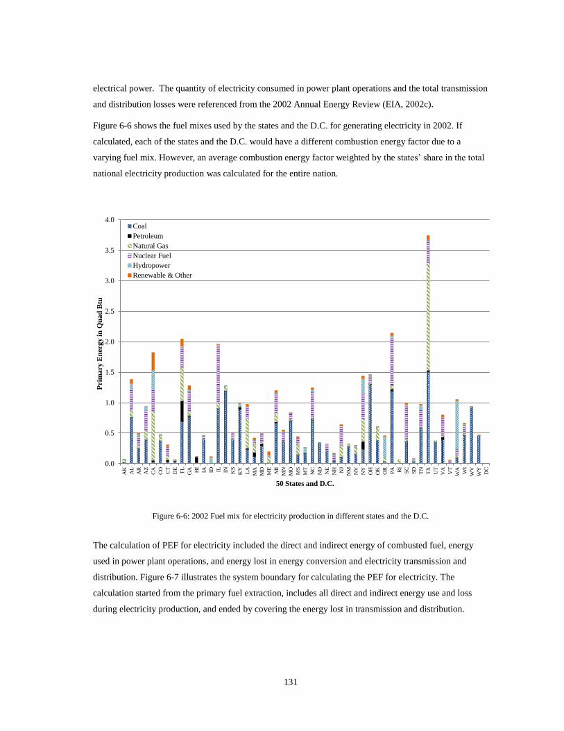
131
electrical power. The quantity of electricity consumed in power plant operations and the total transmission
and distribution losses were referenced from the 2002 Annual Energy Review (EIA, 2002c).
Figure 6-6 shows the fuel mixes used by the states and the D.C. for generating electricity in 2002. If
calculated, each of the states and the D.C. would have a different combustion energy factor due to a
varying fuel mix. However, an average combustion energy factor weighted by the states’ share in the total
national electricity production was calculated for the entire nation.
Figure 6-6: 2002 Fuel mix for electricity production in different states and the D.C.
The calculation of PEF for electricity included the direct and indirect energy of combusted fuel, energy
used in power plant operations, and energy lost in energy conversion and electricity transmission and
distribution. Figure 6-7 illustrates the system boundary for calculating the PEF for electricity. The
calculation started from the primary fuel extraction, includes all direct and indirect energy use and loss
during electricity production, and ended by covering the energy lost in transmission and distribution.
0.0
0.5
1.0
1.5
2.0
2.5
3.0
3.5
4.0
AK
AL
AR
AZ
CA
CO
CT
DE
FL
GA HI
IA ID IL IN KS
KY
LA
MA
MD
ME
MI
MN
MO
MS
MT
NC
ND
NE
NH NJ
NM
NV
NY
OH
OK
OR
PA RI
SC
SD
TN
TX
UT
VA
VT
WA
WI
WV
WY
DC
Prim
ary
En
erg
y in
Qu
ad
Btu
50 States and D.C.
Coal
Petroleum
Natural Gas
Nuclear Fuel
Hydropower
Renewable & Other

132
Figure 6-7: System boundary for PEF calculation for electricity
Deru and Torcellini (2007) proposed an approach for calculating the PEF of electricity in the United
States. According to this procedure, three energy components, namely combustion energy, pre-combustion
energy, and the total energy loss were included in the calculation of PEF. The combustion energy
represented a direct energy component, which is the energy of fuel being combusted in a power plant. The
pre-combustion energy included all energy consumed in the upstream processes of extracting, processing,
converting, and delivering primary fuels to the power plant. Both of these energy components also had an
indirect fraction that resulted from the energy and nonenergy requirements of the energy providing sectors.
The total amount of energy lost in the process of transmission and distribution of electricity was also
accounted for in the calculation. To calculate the combustion energy factor, the approach suggested by
Deru and Torcellini (2007) was applied, whereas to calculate the indirect component, the calculated values
of PEF of primary fuels were used. To compute the combustion energy factors, the following information
and variables were used (based on Deru and Torcellini, 2007):
Eo - Total annual net generation of electricity in the United States
Ej - Total annual generation of electricity by states
EFC, i, j - Combustion energy factor by fuel or energy type and region
EFC, j - Combustion primary energy factor for electricity by region
Ltd - Ratio of transmission and distribution losses to total electricity generation
PEFelec - Total primary energy factor for delivered electricity
Qi,j - Quantity of energy of fuel used for electricity generation by fuel or energy type and region
133
δi, j - Fraction of total electricity generation by fuel or energy type and region
ϑi, j - Combustion energy factor for a unit of composite electricity by fuel/energy type and region
εi, j - Electricity generation by fuel or energy type and region
εpe - Total plant energy used
CEFe - Combustion energy factor for all fuels
CEFpe - Combustion energy factor for plant energy
CEFelec - Combustion energy factor for electricity
PCFelec - Pre-combustion energy factor for electricity
FRFin, i - Indirect fuel requirement factor by fuels
Qi - Quantity of energy of fuel used for electricity generation by fuels
Lelec - Energy loss factor for electricity
Qloss - Energy of electricity lost during transmission and distribution
i - Represents an energy source or a fuel
j - Represents a region
6.4.6.1 Combustion Energy Factor Calculation: Electricity
Apart from four major fossil fuel sectors that provided primary fuels to the electricity generating sector,
the gold, silver, and other metal ore mining sector consisted of a subsector that extracted the uranium used
as nuclear fuel by the nuclear power plants. The total amount of uranium extracted, processed and
consumed domestically for generating electricity was used to disaggregate the sector to calculate the
indirect energy use for nuclear fuel.
∑
∑
Equation 6-8
Equation 6-9
Equation 6-10
134
6.4.6.2 Pre-combustion Energy Factor Calculation: Electricity
The pre-combustion energy of fuels combusted for electricity generation was calculated by multiplying
their quantities to their indirect fuel requirement factor. The indirect fuel requirement factor of a fuel was
equal to its PEF minus one (see Equation 6-11). No input-output data was used for the purpose of
calculating the pre-combustion energy factor to avoid double counting of fuel inputs. Major fuels that were
considered in the calculation included coal, natural gas, petroleum, and nuclear fuel, as these fuels together
constituted over 94% of the energy used for generating electricity in 2002. It was assumed that the PEF for
all other fuels including renewable energy sources was one. The following calculations were done to
derive pre-combustion energy factor:
Equation 6-11
∑
Equation 6-12
Q represents the total pre-combustion energy of electricity production.
6.4.6.3 Primary Energy Factor Calculation: Electricity
An energy loss factor for electricity was derived using the total transmission and distribution loss data for
2002. The calculated values of the combustion and pre-combustion energy factors were summed and
multiplied by the energy loss factor to derive the PEF for electricity production.
Equation 6-13
Equation 6-14
The calculation steps discussed so far were for the first approach. In the second approach, the monetary
flows from the energy providing sectors to other industry sectors were replaced by the direct energy
process data. The energy inputs to all five energy providing sectors were also replaced with the process
data. As some energy uses (e.g., energy used in repressuring reservoir) and energy losses (e.g., T&D
losses) did not show up in the input-output table, the calculated PEFs were adjusted to accommodate these
inputs. The PEFs calculated for major fuels were used to compute the PEF for electricity. The third
approach was purely input-output-based. In this approach, the total requirement matrix was used to
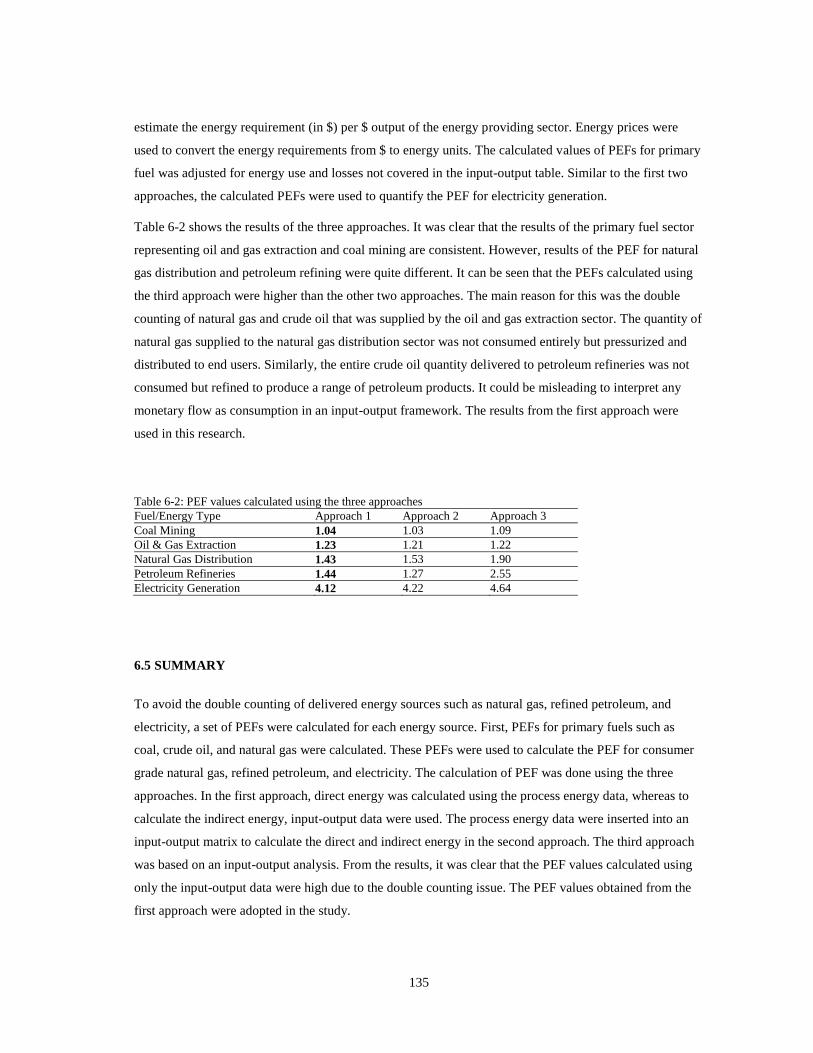
135
estimate the energy requirement (in $) per $ output of the energy providing sector. Energy prices were
used to convert the energy requirements from $ to energy units. The calculated values of PEFs for primary
fuel was adjusted for energy use and losses not covered in the input-output table. Similar to the first two
approaches, the calculated PEFs were used to quantify the PEF for electricity generation.
Table 6-2 shows the results of the three approaches. It was clear that the results of the primary fuel sector
representing oil and gas extraction and coal mining are consistent. However, results of the PEF for natural
gas distribution and petroleum refining were quite different. It can be seen that the PEFs calculated using
the third approach were higher than the other two approaches. The main reason for this was the double
counting of natural gas and crude oil that was supplied by the oil and gas extraction sector. The quantity of
natural gas supplied to the natural gas distribution sector was not consumed entirely but pressurized and
distributed to end users. Similarly, the entire crude oil quantity delivered to petroleum refineries was not
consumed but refined to produce a range of petroleum products. It could be misleading to interpret any
monetary flow as consumption in an input-output framework. The results from the first approach were
used in this research.
Table 6-2: PEF values calculated using the three approaches
Fuel/Energy Type Approach 1 Approach 2 Approach 3
Coal Mining 1.04 1.03 1.09
Oil & Gas Extraction 1.23 1.21 1.22
Natural Gas Distribution 1.43 1.53 1.90
Petroleum Refineries 1.44 1.27 2.55
Electricity Generation 4.12 4.22 4.64
6.5 SUMMARY
To avoid the double counting of delivered energy sources such as natural gas, refined petroleum, and
electricity, a set of PEFs were calculated for each energy source. First, PEFs for primary fuels such as
coal, crude oil, and natural gas were calculated. These PEFs were used to calculate the PEF for consumer
grade natural gas, refined petroleum, and electricity. The calculation of PEF was done using the three
approaches. In the first approach, direct energy was calculated using the process energy data, whereas to
calculate the indirect energy, input-output data were used. The process energy data were inserted into an
input-output matrix to calculate the direct and indirect energy in the second approach. The third approach
was based on an input-output analysis. From the results, it was clear that the PEF values calculated using
only the input-output data were high due to the double counting issue. The PEF values obtained from the
first approach were adopted in the study.
136
CHAPTER VII
HUMAN AND CAPITAL ENERGY CALCULATION
7.
7.1 HUMAN ENERGY
The process of manufacturing and construction are labor intensive and the energy embodied in labor needs
to be included in embodied energy calculations. In some regions of the world, the industry sectors such as,
manufacturing, construction, mining, agriculture, and business employ extensive labor due to low wages,
high labor availability, and limited energy sources. If the final products are to be compared in embodied
energy terms, it should be ensured that both the mechanical and human energy are accounted for. The
energy requirements of human labor vary with factors such as age, sex, weight, lifestyle, and also the
socio-economic conditions (FAO, 2001; Held, 2010). The energy requirements of labor can be categorized
in three parts. The first part is the energy required to perform the basal metabolism that is a series of basic
body functions such as respiration, brain function, body temperature maintenance, secretion of hormones
and enzymes, and heart and lung functions. This fraction represents the threshold of energy that is required
for the basic functioning of a human body and is termed basal metabolic rate (BMR). According to FAO
(2001), the BMR could represent up to 45-70% of the total daily energy requirements of a human body.
The second part includes the energy required to eat and digest the food, and to absorb, transform,
transport, and deposit essential nutrients. This fraction is known as the metabolic response to food and
could constitute energy up to 10% of the BMR. The third part relates to the activity an individual is
engaged in. Depending upon the activities such as exercising, biking, working in an office, loading and
unloading, and working in a manufacturing unit, the energy requirement may vary. Human beings are
engaged in physical activities that are either obligatory or discretionary. The obligatory activities can
hardly be avoided due to the socio-economic and cultural settings. Discretionary activities are the
activities an individual is not obligated to engage in due to social, economic, and cultural settings. In
addition, other human body functions such as growth of tissues also need energy. The following
definitions are important to know (FAO, 2001; Held, 2010):
Total Energy Expenditure (TEE): The average amount of total energy expended by an individual in 24
hours of a typical day.
Basal Metabolic Rate (BMR): The minimum energy rate required to support the basal metabolism,
measured in an individual who is awake, immobile, thermo-neutral, mentally relaxed, is in a supine
position, has rested for at least 8 hours, and fasted for a minimum 12 hours. The rate of energy required is
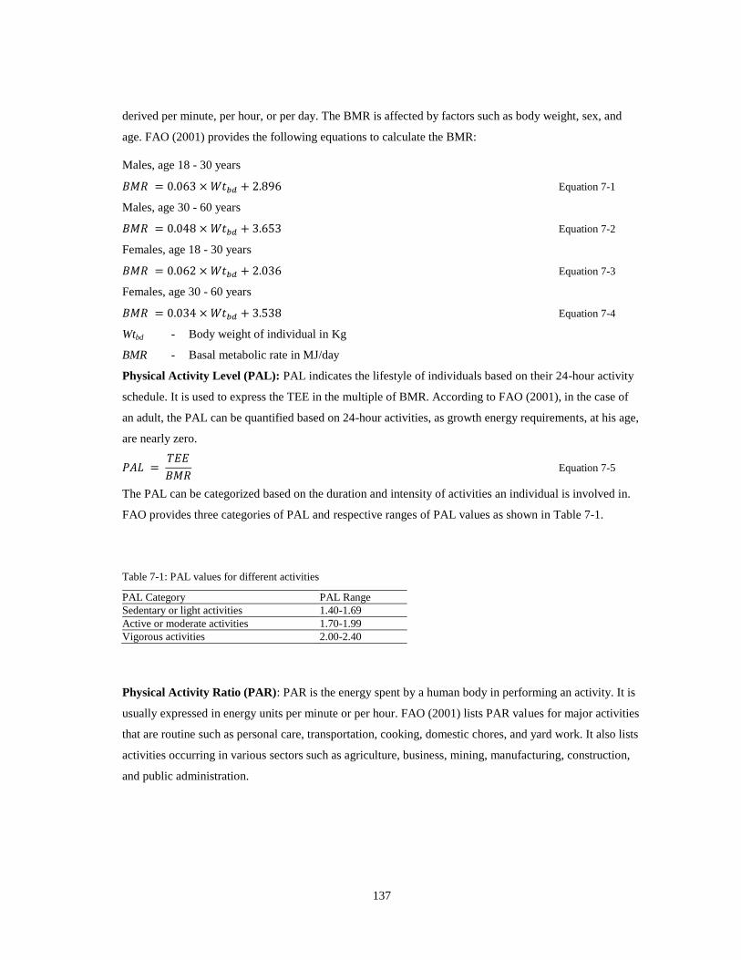
137
derived per minute, per hour, or per day. The BMR is affected by factors such as body weight, sex, and
age. FAO (2001) provides the following equations to calculate the BMR:
Males, age 18 - 30 years
Equation 7-1
Males, age 30 - 60 years
Equation 7-2
Females, age 18 - 30 years
Equation 7-3
Females, age 30 - 60 years
Equation 7-4
Wtbd - Body weight of individual in Kg
BMR - Basal metabolic rate in MJ/day
Physical Activity Level (PAL): PAL indicates the lifestyle of individuals based on their 24-hour activity
schedule. It is used to express the TEE in the multiple of BMR. According to FAO (2001), in the case of
an adult, the PAL can be quantified based on 24-hour activities, as growth energy requirements, at his age,
are nearly zero.
Equation 7-5
The PAL can be categorized based on the duration and intensity of activities an individual is involved in.
FAO provides three categories of PAL and respective ranges of PAL values as shown in Table 7-1.
Table 7-1: PAL values for different activities
PAL Category PAL Range
Sedentary or light activities 1.40-1.69
Active or moderate activities 1.70-1.99
Vigorous activities 2.00-2.40
Physical Activity Ratio (PAR): PAR is the energy spent by a human body in performing an activity. It is
usually expressed in energy units per minute or per hour. FAO (2001) lists PAR values for major activities
that are routine such as personal care, transportation, cooking, domestic chores, and yard work. It also lists
activities occurring in various sectors such as agriculture, business, mining, manufacturing, construction,
and public administration.
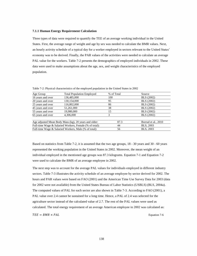
138
7.1.1 Human Energy Requirement Calculation
Three types of data were required to quantify the TEE of an average working individual in the United
States. First, the average range of weight and age by sex was needed to calculate the BMR values. Next,
an hourly activity schedule of a typical day for a worker employed in sectors relevant to the United States’
economy was to be derived. Finally, the PAR values of the activities were needed to calculate an average
PAL value for the workers. Table 7-2 presents the demographics of employed individuals in 2002. These
data were used to make assumptions about the age, sex, and weight characteristics of the employed
population.
Table 7-2: Physical characteristics of the employed population in the United States in 2002
Age Group Total Population Employed % of Total Source
16 years and over 136,485,000 100 BLS (2002)
20 years and over 130,154,000 95 BLS (2002)
25 years and over 116,802,000 86 BLS (2002)
45 years and over 51,261,000 38 BLS (2002)
55 years and over 19,980,000 15 BLS (2002)
65 years and over 4,306,000 3 BLS (2002)
Age adjusted Mean Body Mass (kg), 20 years and older: 87.3 Borrud et al., 2010
Full-time Wage & Salaried Workers, Female (% of total): 44 BLS, 2003
Full-time Wage & Salaried Workers, Male (% of total): 56 BLS, 2003
Based on statistics from Table 7-2, it is assumed that the two age groups, 18 - 30 years and 30 - 60 years
represented the working population in the United States in 2002. Moreover, the mean weight of an
individual employed in the mentioned age groups was 87.3 kilograms. Equation 7-1 and Equation 7-2
were used to calculate the BMR of an average employee in 2002.
The next step was to account for the average PAL values for individuals employed in different industry
sectors. Table 7-3 illustrates the activity schedule of an average employee by sector derived for 2002. The
hours and PAR values were based on FAO (2001) and the American Time Use Survey Data for 2003 (data
for 2002 were not available) from the United States Bureau of Labor Statistics (USBLS) (BLS, 2004a).
The computed values of PAL for each sector are also shown in Table 7-3. According to FAO (2001), a
PAL value over 2.4 cannot be sustained for a long time. Hence, a PAL of 2.4 was selected for the
agriculture sector instead of the calculated value of 2.7. The rest of the PAL values were used as
calculated. The total energy requirement of an average American employee in 2002 was calculated as:
Equation 7-6
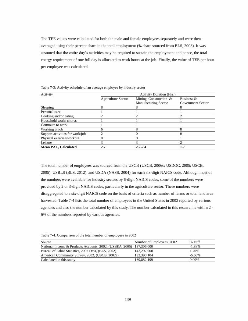
139
The TEE values were calculated for both the male and female employees separately and were then
averaged using their percent share in the total employment (% share sourced from BLS, 2003). It was
assumed that the entire day’s activities may be required to sustain the employment and hence, the total
energy requirement of one full day is allocated to work hours at the job. Finally, the value of TEE per hour
per employee was calculated.
Table 7-3: Activity schedule of an average employee by industry sector
Activity Activity Duration (Hrs.)
Agriculture Sector Mining, Construction &
Manufacturing Sector
Business &
Government Sector
Sleeping 8 8 8
Personal care 1 1 1
Cooking and/or eating 2 2 2
Household work/ chores 1 1 1
Commute to work 1 1 1
Working at job 6 8 8
Support activities for work/job 2 0 0
Physical exercise/workout 0 0 1
Leisure 3 3 2
Mean PAL, Calculated 2.7 2.2-2.4 1.7
The total number of employees was sourced from the USCB (USCB, 2006c; USDOC, 2005; USCB,
2005), USBLS (BLS, 2012), and USDA (NASS, 2004) for each six-digit NAICS code. Although most of
the numbers were available for industry sectors by 6-digit NAICS codes, some of the numbers were
provided by 2 or 3-digit NAICS codes, particularly in the agriculture sector. These numbers were
disaggregated to a six-digit NAICS code on the basis of criteria such as number of farms or total land area
harvested. Table 7-4 lists the total number of employees in the United States in 2002 reported by various
agencies and also the number calculated by this study. The number calculated in this research is within 2 -
6% of the numbers reported by various agencies.
Table 7-4: Comparison of the total number of employees in 2002
Source Number of Employees, 2002 % Diff
National Income & Products Accounts, 2002, (USBEA, 2005) 137,306,000 -1.88%
Bureau of Labor Statistics, 2002 Data, (BLS, 2002) 142,297,000 1.70%
American Community Survey, 2002, (USCB, 2002a) 132,390,104 -5.66%
Calculated in this study 139,882,199 0.00%

140
It was important to make a distinction between the production workers and other staff due to their varying
daily energy requirements. The USBLS reported the number of employees as well as the number of
production workers (USBLS, 2012). The total energy requirements calculated on the basis of Table 7-3
should be applied to production workers only. The remaining employees were assumed as technical or
managerial staff and their TEE was derived using a PAL value of 1.7. The total annual energy consumed
by an individual employee was calculated by multiplying the per hour TEE values to the annual work
hours data (per employee) provided by the USBLS by industry sector (USBLS, 2012).
The number of employees who worked for the industry also used private transportation to commute to
work. The inputs and outputs used by private households were not a part of the direct and total
requirement matrix. The private transportation used by individuals was not accounted for in calculating the
energy use of various transportation sectors. Hence, the transportation energy consumed by each
individual employee, who commuted to work using private vehicles, needs to be included in the total
human energy. In addition, a fraction of the total expenditure of an average household belonged to the
industry of employment. Expenses on items such as clothes, accessories, housing, appliances, automobile,
and health should also be allotted to the employment industry (Cleveland and Costanza, 2008). How
should we allocate these expenses to the industry of employment? Cleveland and Costanza (2008)
suggested that the difference between the expenses of an earner and non-earner can be used to identify
expenses incurred due to the employment.
The transportation energy data for 2002 were sourced from the USDOT (USDOT, 2012). The total energy
consumed by cars and light trucks in 2002 was 21,410 trillion Btu. A fraction of this energy was consumed
by taxicabs and other rental vehicles, which should be subtracted in order to estimate the energy
specifically used by personal vehicles. The fraction of taxicabs and rental vehicles was calculated from the
National Transportation Statistics data published by the USDOT (USDOT, 2012). The transportation
energy of personal vehicles was estimated to be nearly 13 quadrillion Btu. Not all of the personal
transportation was used for work related purposes. The Federal Highway Administration (USDOT)
published data on work-related trips for the years 1983, 1990, 1995, 2001, and 2009 (Santos et al., 2011).
Figure 7-1 shows the trends of work related trips by Vehicle Miles of Travel (VMT) and Person Miles of
Travel (PMT). The percentage of total work-related trips was consistently between 22 - 30% of the total
trips. For 2002, 27% of the total trips were considered work-related and 27% of the energy consumed in
personal transportation was allocated to the industry of employment (Santos et al., 2011).
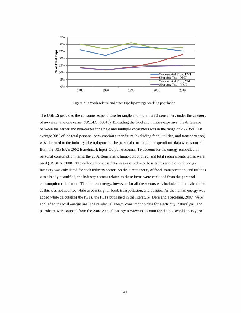
141
Figure 7-1: Work-related and other trips by average working population
The USBLS provided the consumer expenditure for single and more than 2 consumers under the category
of no earner and one earner (USBLS, 2004b). Excluding the food and utilities expenses, the difference
between the earner and non-earner for single and multiple consumers was in the range of 26 - 35%. An
average 30% of the total personal consumption expenditure (excluding food, utilities, and transportation)
was allocated to the industry of employment. The personal consumption expenditure data were sourced
from the USBEA’s 2002 Benchmark Input-Output Accounts. To account for the energy embodied in
personal consumption items, the 2002 Benchmark Input-output direct and total requirements tables were
used (USBEA, 2008). The collected process data was inserted into these tables and the total energy
intensity was calculated for each industry sector. As the direct energy of food, transportation, and utilities
was already quantified, the industry sectors related to these items were excluded from the personal
consumption calculation. The indirect energy, however, for all the sectors was included in the calculation,
as this was not counted while accounting for food, transportation, and utilities. As the human energy was
added while calculating the PEFs, the PEFs published in the literature (Deru and Torcellini, 2007) were
applied to the total energy use. The residential energy consumption data for electricity, natural gas, and
petroleum were sourced from the 2002 Annual Energy Review to account for the household energy use.
0%
5%
10%
15%
20%
25%
30%
35%
1983 1990 1995 2001 2009
% o
f T
ota
l T
rip
s
Work-related Trips, PMTShopping Trips, PMTWork-related Trips, VMTShopping Trips, VMT
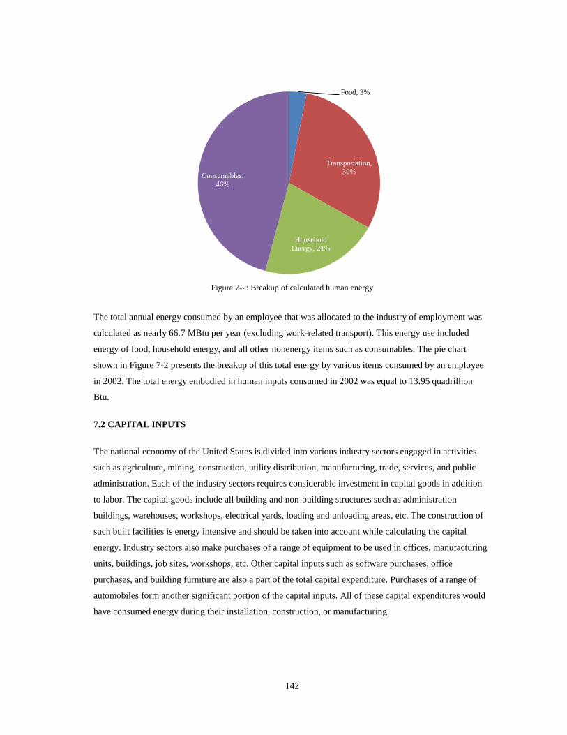
142
Figure 7-2: Breakup of calculated human energy
The total annual energy consumed by an employee that was allocated to the industry of employment was
calculated as nearly 66.7 MBtu per year (excluding work-related transport). This energy use included
energy of food, household energy, and all other nonenergy items such as consumables. The pie chart
shown in Figure 7-2 presents the breakup of this total energy by various items consumed by an employee
in 2002. The total energy embodied in human inputs consumed in 2002 was equal to 13.95 quadrillion
Btu.
7.2 CAPITAL INPUTS
The national economy of the United States is divided into various industry sectors engaged in activities
such as agriculture, mining, construction, utility distribution, manufacturing, trade, services, and public
administration. Each of the industry sectors requires considerable investment in capital goods in addition
to labor. The capital goods include all building and non-building structures such as administration
buildings, warehouses, workshops, electrical yards, loading and unloading areas, etc. The construction of
such built facilities is energy intensive and should be taken into account while calculating the capital
energy. Industry sectors also make purchases of a range of equipment to be used in offices, manufacturing
units, buildings, job sites, workshops, etc. Other capital inputs such as software purchases, office
purchases, and building furniture are also a part of the total capital expenditure. Purchases of a range of
automobiles form another significant portion of the capital inputs. All of these capital expenditures would
have consumed energy during their installation, construction, or manufacturing.
Food, 3%
Transportation,
30%
Household
Energy, 21%
Consumables,
46%
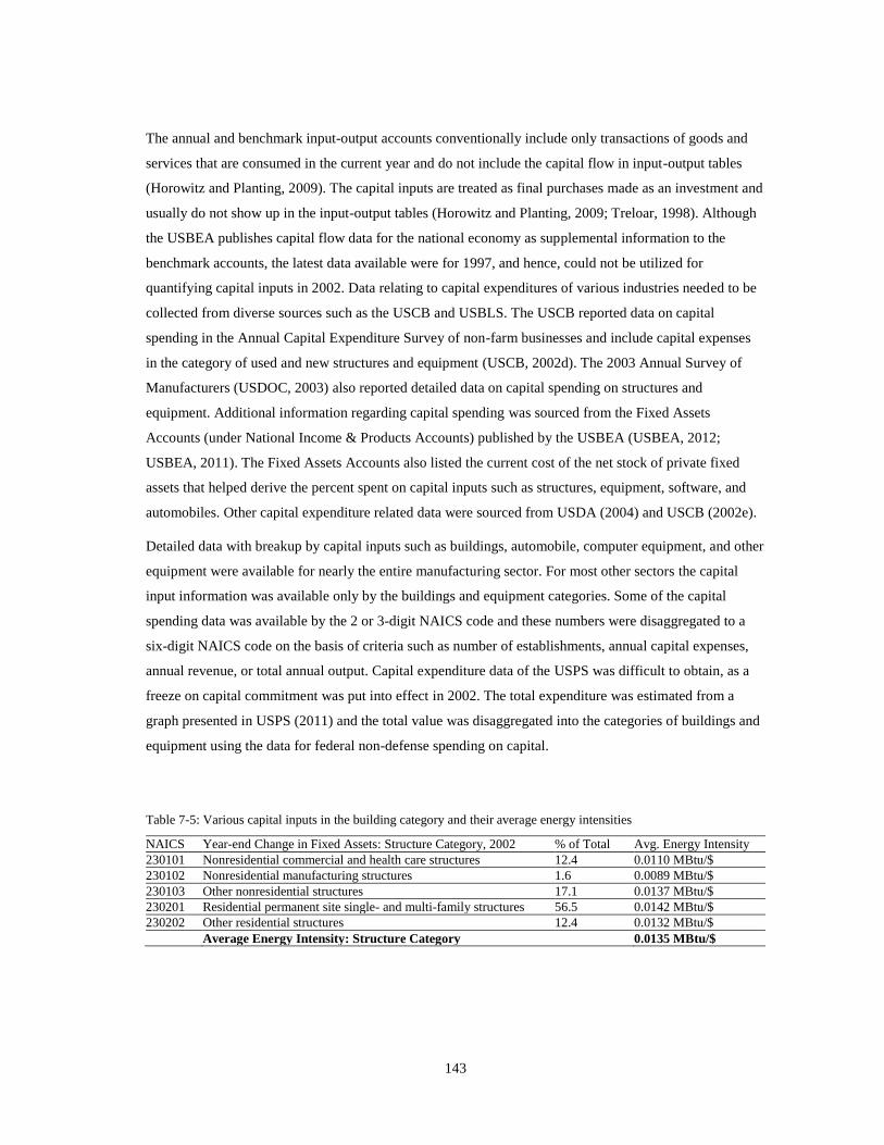
143
The annual and benchmark input-output accounts conventionally include only transactions of goods and
services that are consumed in the current year and do not include the capital flow in input-output tables
(Horowitz and Planting, 2009). The capital inputs are treated as final purchases made as an investment and
usually do not show up in the input-output tables (Horowitz and Planting, 2009; Treloar, 1998). Although
the USBEA publishes capital flow data for the national economy as supplemental information to the
benchmark accounts, the latest data available were for 1997, and hence, could not be utilized for
quantifying capital inputs in 2002. Data relating to capital expenditures of various industries needed to be
collected from diverse sources such as the USCB and USBLS. The USCB reported data on capital
spending in the Annual Capital Expenditure Survey of non-farm businesses and include capital expenses
in the category of used and new structures and equipment (USCB, 2002d). The 2003 Annual Survey of
Manufacturers (USDOC, 2003) also reported detailed data on capital spending on structures and
equipment. Additional information regarding capital spending was sourced from the Fixed Assets
Accounts (under National Income & Products Accounts) published by the USBEA (USBEA, 2012;
USBEA, 2011). The Fixed Assets Accounts also listed the current cost of the net stock of private fixed
assets that helped derive the percent spent on capital inputs such as structures, equipment, software, and
automobiles. Other capital expenditure related data were sourced from USDA (2004) and USCB (2002e).
Detailed data with breakup by capital inputs such as buildings, automobile, computer equipment, and other
equipment were available for nearly the entire manufacturing sector. For most other sectors the capital
input information was available only by the buildings and equipment categories. Some of the capital
spending data was available by the 2 or 3-digit NAICS code and these numbers were disaggregated to a
six-digit NAICS code on the basis of criteria such as number of establishments, annual capital expenses,
annual revenue, or total annual output. Capital expenditure data of the USPS was difficult to obtain, as a
freeze on capital commitment was put into effect in 2002. The total expenditure was estimated from a
graph presented in USPS (2011) and the total value was disaggregated into the categories of buildings and
equipment using the data for federal non-defense spending on capital.
Table 7-5: Various capital inputs in the building category and their average energy intensities
NAICS Year-end Change in Fixed Assets: Structure Category, 2002 % of Total Avg. Energy Intensity
230101 Nonresidential commercial and health care structures 12.4 0.0110 MBtu/$
230102 Nonresidential manufacturing structures 1.6 0.0089 MBtu/$
230103 Other nonresidential structures 17.1 0.0137 MBtu/$
230201 Residential permanent site single- and multi-family structures 56.5 0.0142 MBtu/$
230202 Other residential structures 12.4 0.0132 MBtu/$
Average Energy Intensity: Structure Category 0.0135 MBtu/$

144
After gathering the capital spending data for all relevant sectors, the total capital spending was roughly
1204 billion dollars. This amount was verified by calculating the change in the fixed assets value from the
USBEA’s Fixed Assets Accounts (USBEA, 2011). The change in fixed assets at the end of 2002 was
reported at roughly 1165 billion dollars, which is within 3.5% of the calculated value. The breakup of
change in year-end fixed assets from 2001 to 2002 in the equipment and building categories was used to
calculate the energy intensity for building and equipment category. The energy intensity was averaged on
the basis of relative share of capital inputs in the total net change in the fixed assets’ value at the end of
2002. Table 7-5 and Table 7-6 show the breakup of the structure and equipment categories with their
average energy intensities and percent share in the total change in the value of fixed assets.
The total energy embodied in capital inputs at the end of 2002 was calculated as 16.3 quadrillion Btu. The
share of equipment and structure in the total capital energy was equal to 8.4 and 7.9 quadrillion Btu,
respectively. A more detailed account of capital flow was needed in order to quantify the capital energy
more accurately and consistently. If the capital flow accounts were published concurrently with the
national input-output accounts, it would be easier to accurately calculate the energy embodied in capital
expenditure. It was interesting to know that the energy intensities of capital equipment and structure input
were nearly the same. Although the economic input-output framework was used for the calculation, the
input-output energy data were replaced by the process energy data.
Table 7-6: Other capital inputs and their average energy intensities
NAICS Yearend Change in Fixed Assets: Equipment Category, 2002 % of Total Avg. Energy
intensity
334 Computer and Electronic Product Manufacturing 17.3 0.0110 MBtu/$
3391 Medical Equipment and Supplies Manufacturing 18.3 0.0103 MBtu/$
333293 Printing Machinery and Equipment Manufacturing 0.3 0.0141 MBtu/$
3332 Industrial Machinery Manufacturing
20.2 0.0149 MBtu/$
3334 Ventilation, Heating, Air-Conditioning, and Commercial Refrigeration
Equipment Manufacturing
3335 Metalworking Machinery Manufacturing
3336 Engine, Turbine, and Power Transmission Equipment Manufacturing
3339 Other General Purpose Machinery Manufacturing
3353 Electrical Equipment Manufacturing
3359 Other Electrical Equipment and Component Manufacturing
336 Transportation Equipment Manufacturing 11.4 0.0141 MBtu/$
3331 Agriculture, Construction, and Mining Machinery Manufacturing 4.6 0.0153 MBtu/$
3333 Commercial and Service Industry Machinery Manufacturing 16.6 0.0145 MBtu/$
3351 Electric Lighting Equipment Manufacturing 1.0 0.0171 MBtu/$
3352 Household Appliance Manufacturing
3371 Household and Institutional Furniture and Kitchen Cabinet Manufacturing 10.3 0.0170 MBtu/$
3372 Office Furniture (including Fixtures) Manufacturing
Average Energy Intensity: Equipment/Other Category 0.0135 MBtu/$

145
7.3 SUMMARY
The calculation of human energy involved three components, namely energy of food, energy of
consumables, and household energy use. The amount of food energy consumed by an individual depends
upon various factors such as age, gender, and body mass. To calculate the energy of food consumed by an
average worker, a national average for age and body mass was derived. A schedule of activities was also
established for various work categories such as farming, labor, office work, etc. Using the average
physical parameters for the 2002 working population and its activity schedule, the energy of food was
quantified. The energy embodied in other consumables was calculated using the 2002 personal
consumption expenditure data and input-output-based energy intensities. The energy used by an average
household was sourced from the 2002 Annual Energy Review. The fraction of the total energy consumed
by an average working individual that can be attributed to the employment was calculated as 67 MBtu per
year excluding transportation. The energy embodied in capital investments was calculated by gathering the
capital investment data by categories such as structure, equipment, automobile, and software. Using the
input-output-based energy intensities, the total energy embodied in capital goods was quantified. Overall,
nearly 16 quadrillion Btu of capital energy was consumed in the United States in 2002. Although, the data
on total capital investment was gathered from a variety of sources, availability of capital input accounts in
a timely manner would certainly improve the quality of capital input data in the future.
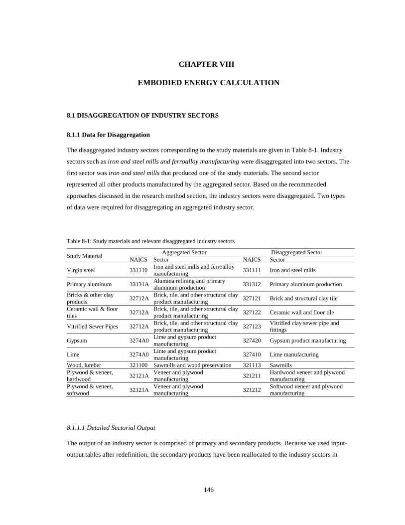
146
CHAPTER VIII
EMBODIED ENERGY CALCULATION
8.
8.1 DISAGGREGATION OF INDUSTRY SECTORS
8.1.1 Data for Disaggregation
The disaggregated industry sectors corresponding to the study materials are given in Table 8-1. Industry
sectors such as iron and steel mills and ferroalloy manufacturing were disaggregated into two sectors. The
first sector was iron and steel mills that produced one of the study materials. The second sector
represented all other products manufactured by the aggregated sector. Based on the recommended
approaches discussed in the research method section, the industry sectors were disaggregated. Two types
of data were required for disaggregating an aggregated industry sector.
Table 8-1: Study materials and relevant disaggregated industry sectors
Study Material Aggregated Sector Disaggregated Sector
NAICS Sector NAICS Sector
Virgin steel 331110 Iron and steel mills and ferroalloy
manufacturing 331111 Iron and steel mills
Primary aluminum 33131A Alumina refining and primary
aluminum production 331312 Primary aluminum production
Bricks & other clay
products 32712A
Brick, tile, and other structural clay
product manufacturing 327121 Brick and structural clay tile
Ceramic wall & floor
tiles 32712A
Brick, tile, and other structural clay
product manufacturing 327122 Ceramic wall and floor tile
Vitrified Sewer Pipes 32712A Brick, tile, and other structural clay
product manufacturing 327123
Vitrified clay sewer pipe and
fittings
Gypsum 3274A0 Lime and gypsum product
manufacturing 327420 Gypsum product manufacturing
Lime 3274A0 Lime and gypsum product
manufacturing 327410 Lime manufacturing
Wood, lumber 321100 Sawmills and wood preservation 321113 Sawmills
Plywood & veneer,
hardwood 32121A
Veneer and plywood
manufacturing 321211
Hardwood veneer and plywood
manufacturing
Plywood & veneer,
softwood 32121A
Veneer and plywood
manufacturing 321212
Softwood veneer and plywood
manufacturing
8.1.1.1 Detailed Sectorial Output
The output of an industry sector is comprised of primary and secondary products. Because we used input-
output tables after redefinition, the secondary products have been reallocated to the industry sectors in
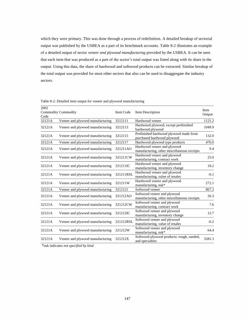
147
which they were primary. This was done through a process of redefinition. A detailed breakup of sectorial
output was published by the USBEA as a part of its benchmark accounts. Table 8-2 illustrates an example
of a detailed output of sector veneer and plywood manufacturing provided by the USBEA. It can be seen
that each item that was produced as a part of the sector’s total output was listed along with its share in the
output. Using this data, the share of hardwood and softwood products can be extracted. Similar breakup of
the total output was provided for most other sectors that also can be used to disaggregate the industry
sectors.
Table 8-2: Detailed item output for veneer and plywood manufacturing
2002
Commodity
Code
Commodity Item Code Item Description Item
Output
32121A Veneer and plywood manufacturing 3212111 Hardwood veneer 1121.2
32121A Veneer and plywood manufacturing 3212113 Hardwood plywood, except prefinished
hardwood plywood 1049.9
32121A Veneer and plywood manufacturing 3212115 Prefinished hardwood plywood made from
purchased hardwood plywood 132.0
32121A Veneer and plywood manufacturing 3212117 Hardwood plywood type products 476.0
32121A Veneer and plywood manufacturing 321211AO Hardwood veneer and plywood
manufacturing, other miscellaneous receipts 9.4
32121A Veneer and plywood manufacturing 321211CW Hardwood veneer and plywood
manufacturing, contract work 25.0
32121A Veneer and plywood manufacturing 321211IC Hardwood veneer and plywood
manufacturing, inventory change 18.2
32121A Veneer and plywood manufacturing 321211RSL Hardwood veneer and plywood
manufacturing, value of resales -0.1
32121A Veneer and plywood manufacturing 321211W Hardwood veneer and plywood
manufacturing, nsk* 272.1
32121A Veneer and plywood manufacturing 3212121 Softwood veneer 867.2
32121A Veneer and plywood manufacturing 321212AO Softwood veneer and plywood
manufacturing, other miscellaneous receipts 26.3
32121A Veneer and plywood manufacturing 321212CW Softwood veneer and plywood
manufacturing, contract work 7.6
32121A Veneer and plywood manufacturing 321212IC Softwood veneer and plywood
manufacturing, inventory change 12.7
32121A Veneer and plywood manufacturing 321212RSL Softwood veneer and plywood
manufacturing, value of resales -0.2
32121A Veneer and plywood manufacturing 321212W Softwood veneer and plywood
manufacturing, nsk* 64.4
32121A Veneer and plywood manufacturing 321212X Softwood plywood products: rough, sanded,
and specialties 3581.3
*nsk indicates not specified by kind
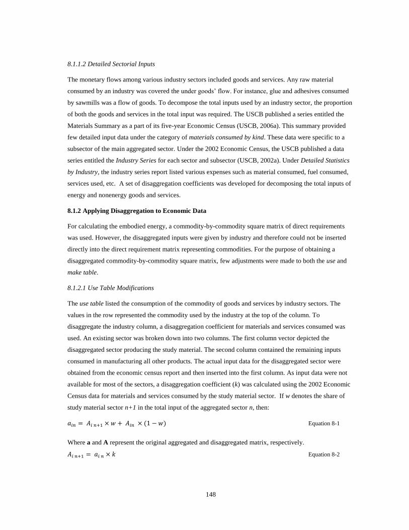
148
8.1.1.2 Detailed Sectorial Inputs
The monetary flows among various industry sectors included goods and services. Any raw material
consumed by an industry was covered the under goods’ flow. For instance, glue and adhesives consumed
by sawmills was a flow of goods. To decompose the total inputs used by an industry sector, the proportion
of both the goods and services in the total input was required. The USCB published a series entitled the
Materials Summary as a part of its five-year Economic Census (USCB, 2006a). This summary provided
few detailed input data under the category of materials consumed by kind. These data were specific to a
subsector of the main aggregated sector. Under the 2002 Economic Census, the USCB published a data
series entitled the Industry Series for each sector and subsector (USCB, 2002a). Under Detailed Statistics
by Industry, the industry series report listed various expenses such as material consumed, fuel consumed,
services used, etc. A set of disaggregation coefficients was developed for decomposing the total inputs of
energy and nonenergy goods and services.
8.1.2 Applying Disaggregation to Economic Data
For calculating the embodied energy, a commodity-by-commodity square matrix of direct requirements
was used. However, the disaggregated inputs were given by industry and therefore could not be inserted
directly into the direct requirement matrix representing commodities. For the purpose of obtaining a
disaggregated commodity-by-commodity square matrix, few adjustments were made to both the use and
make table.
8.1.2.1 Use Table Modifications
The use table listed the consumption of the commodity of goods and services by industry sectors. The
values in the row represented the commodity used by the industry at the top of the column. To
disaggregate the industry column, a disaggregation coefficient for materials and services consumed was
used. An existing sector was broken down into two columns. The first column vector depicted the
disaggregated sector producing the study material. The second column contained the remaining inputs
consumed in manufacturing all other products. The actual input data for the disaggregated sector were
obtained from the economic census report and then inserted into the first column. As input data were not
available for most of the sectors, a disaggregation coefficient (k) was calculated using the 2002 Economic
Census data for materials and services consumed by the study material sector. If w denotes the share of
study material sector n+1 in the total input of the aggregated sector n, then:
Equation 8-1
Where a and A represent the original aggregated and disaggregated matrix, respectively.
Equation 8-2

149
Equation 8-3
The above equations became a constraint for disaggregating an input-output industry sector. The column
vector of the disaggregated sector contained all of its inputs drawn from other industry sectors.
The row entries in the use table contained the value of the row commodity used by the industry at the top
of the column. As the purpose was to create a decomposed commodity-by-commodity square matrix of
direct requirements, it was important to create a row commodity to represent the disaggregated industry
sector n+1. In this study it was assumed that the use of the disaggregated commodity by the column
industries can be depicted by the disaggregated commodity’s share in the total output of the aggregated
commodity.
8.1.2.2 Make Table Modifications
The row entries in the make table represented industries making various commodities listed in the
columns. The row representing the aggregated industry sector n was divided into two rows. The first row
defined the disaggregated industry and its make of column commodities. It was assumed that the share (w)
of the disaggregated industry in the output of the aggregated industry would represent its proportion in
making the column commodities. Therefore, the amount of a commodity produced by the aggregated
sector was multiplied by w to compute the commodities made by the disaggregated sector n+1.The
column vectors of the make table defined the amount of a commodity manufactured by each row industry.
The sum of a column is always 1.0, as each cell in the column is a fraction of commodity produced by
each row. It was considered that the disaggregated commodity was produced in the same proportion as the
original aggregated commodity.
8.2 INSERTING HUMAN AND CAPITAL ENERGY
The calculated values of human and capital energy inputs were for each industry sector. However, we
needed to apply these values to a square matrix representing commodities. Therefore, make table and use
table adjustments were necessary to obtain a commodity-by-commodity direct requirement matrix with
human and capital energy. A new commodity for each, the human and capital input category, was added to
the make table and use table. In the use table there were two new rows with values of human and capital
energy consumed by the industry at the top of the columns. In make table, there were two new columns
representing the make of human and capital energy by industry sectors. As human and capital inputs were
not a part of intermediate transactions, it was assumed that no industry made any of the two inputs. This
meant that all values in the newly added columns of the make table would contain zero entries. The
original 428 X 426 use table matrix now became a 430 X 426 matrix and the 426 X 428 make table matrix
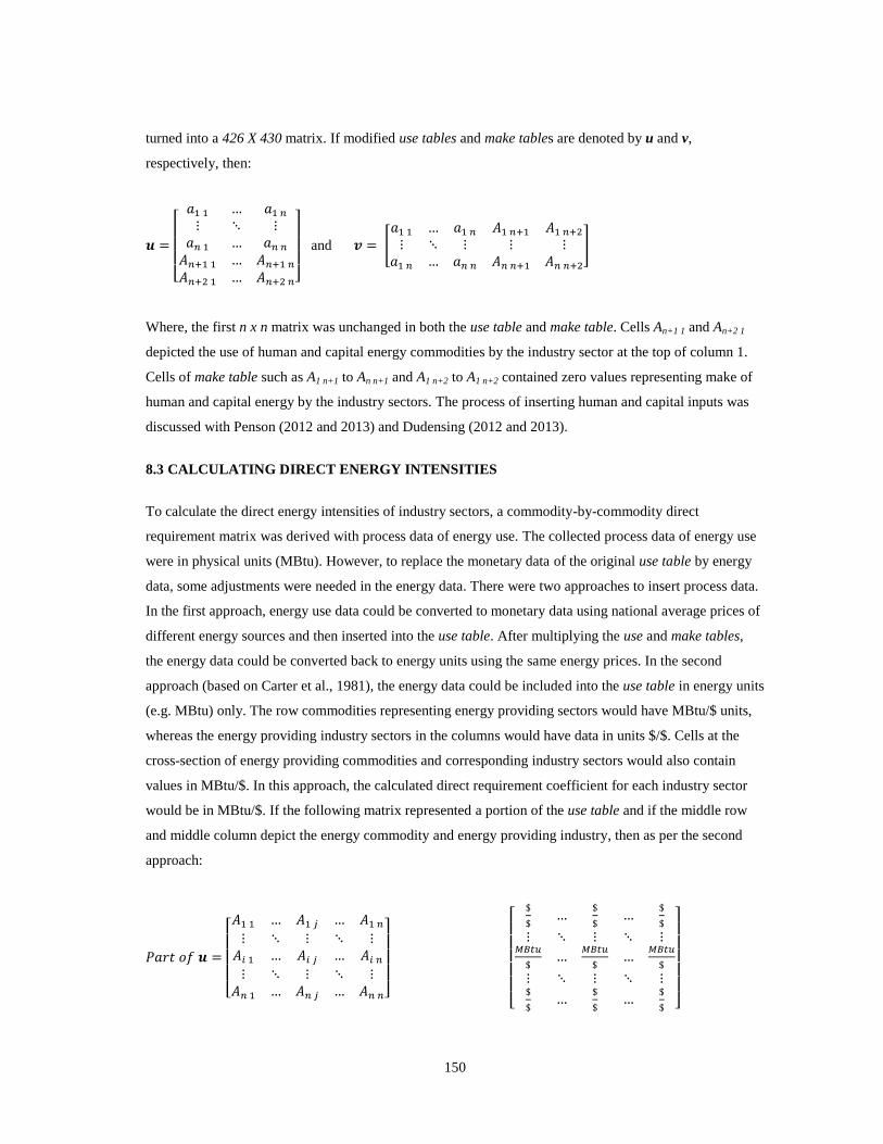
150
turned into a 426 X 430 matrix. If modified use tables and make tables are denoted by u and v,
respectively, then:
[
]
and [
]
Where, the first n x n matrix was unchanged in both the use table and make table. Cells An+1 1 and An+2 1
depicted the use of human and capital energy commodities by the industry sector at the top of column 1.
Cells of make table such as A1 n+1 to An n+1 and A1 n+2 to A1 n+2 contained zero values representing make of
human and capital energy by the industry sectors. The process of inserting human and capital inputs was
discussed with Penson (2012 and 2013) and Dudensing (2012 and 2013).
8.3 CALCULATING DIRECT ENERGY INTENSITIES
To calculate the direct energy intensities of industry sectors, a commodity-by-commodity direct
requirement matrix was derived with process data of energy use. The collected process data of energy use
were in physical units (MBtu). However, to replace the monetary data of the original use table by energy
data, some adjustments were needed in the energy data. There were two approaches to insert process data.
In the first approach, energy use data could be converted to monetary data using national average prices of
different energy sources and then inserted into the use table. After multiplying the use and make tables,
the energy data could be converted back to energy units using the same energy prices. In the second
approach (based on Carter et al., 1981), the energy data could be included into the use table in energy units
(e.g. MBtu) only. The row commodities representing energy providing sectors would have MBtu/$ units,
whereas the energy providing industry sectors in the columns would have data in units $/$. Cells at the
cross-section of energy providing commodities and corresponding industry sectors would also contain
values in MBtu/$. In this approach, the calculated direct requirement coefficient for each industry sector
would be in MBtu/$. If the following matrix represented a portion of the use table and if the middle row
and middle column depict the energy commodity and energy providing industry, then as per the second
approach:
[
]
[
]

151
As the make table provided the fraction of a commodity manufactured by various industries, no changes
were made to the make table. In the second approach, as the energy data were in physical units (MBtu),
not changing the make table meant that the proportions of energy commodities made by industry sectors is
the same in both the monetary and energy units. It can be seen that both the approaches are actually
similar. The only difference is that in the first approach, there is no assumption of commodity fractions in
monetary or energy terms. In this research, we adopted the second approach.
The second matrix shows the various units after inserting process data as per approach two as discussed in
the earlier paragraph. One major advantage of using process data in physical units was that no average
energy prices were used to convert the monetary data into energy intensities. As energy prices may vary
and may not be representative of the actual prices paid by the industries, they could seriously affect the
embodied energy calculations (Crawford, 2004; Acquaye, 2010). By avoiding the use of average energy
prices, the reliability of input-output-based energy analysis was further improved.
After modifying the use table, it was multiplied by the make table to derive a commodity-by-commodity
square matrix of direct requirements. The direct requirement matrix provided the direct energy intensity of
each commodity by five energy providing sectors:
Oil and gas extraction
Coal mining
Electric power generation, transmission, and distribution
Natural gas distribution
Petroleum refineries
In addition, there were two other energy sources, namely human and capital energy. It can be seen that
calculating and using separate energy intensity values for different energy providing sectors eliminates the
error caused by using a single representative energy commodity and a fixed energy price that is a national
average.
8.4 CALCULATING INDIRECT ENERGY INTENSITIES
There were two ways to calculate the indirect fraction of the total energy intensity of an industry sector.
First, it could be calculated using Leontief’s Inverse Matrix that represents the total requirements of the
sectors of an economy. The direct requirement matrix was subtracted from an identity matrix and inverted
to find Leontief’s total requirement matrix. The difference of total and direct requirements would provide
the indirect requirements. However, this approach was like a “black box.” We had no idea how the total
energy was calculated (Treloar, 1998). In other words, we could not determine how much energy is
embodied in each stage upstream of the main product. The second approach utilized the Power Series
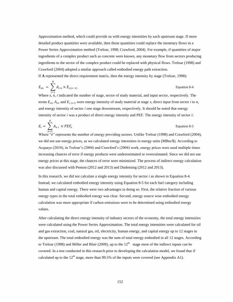
152
Approximation method, which could provide us with energy intensities by each upstream stage. If more
detailed product quantities were available, then those quantities could replace the monetary flows in a
Power Series Approximation method (Treloar, 1998; Crawford, 2004). For example, if quantities of major
ingredients of a complex product such as concrete were known, any monetary flow from sectors producing
ingredients to the sector of the complex product could be replaced with physical flows. Treloar (1998) and
Crawford (2004) adopted a similar approach called embodied energy path extraction.
If A represented the direct requirement matrix, then the energy intensity by stage (Treloar, 1998):
∑
Equation 8-4
Where s, n, i indicated the number of stage, sector of study material, and input sector, respectively. The
terms Esn, Ain, and Ei, (s-1) were energy intensity of study material at stage s, direct input from sector i to n,
and energy intensity of sector i one stage downstream, respectively. It should be noted that energy
intensity of sector i was a product of direct energy intensity and PEF. The energy intensity of sector i:
∑
Equation 8-5
Where “e” represents the number of energy providing sectors. Unlike Treloar (1998) and Crawford (2004),
we did not use energy prices, as we calculated energy intensities in energy units (MBtu/$). According to
Acquaye (2010), in Treloar’s (2004) and Crawford’s (2004) work, energy prices were used multiple times
increasing chances of error if energy products were underestimated or overestimated. Since we did not use
energy prices at this stage, the chances of error were minimized. The process of indirect energy calculation
was also discussed with Penson (2012 and 2013) and Dudensing (2012 and 2013).
In this research, we did not calculate a single energy intensity for sector i as shown in Equation 8-4.
Instead, we calculated embodied energy intensity using Equation 8-5 for each fuel category including
human and capital energy. There were two advantages in doing so. First, the relative fraction of various
energy types in the total embodied energy was clear. Second, energy source wise embodied energy
calculation was more appropriate if carbon emissions were to be determined using embodied energy
values.
After calculating the direct energy intensity of industry sectors of the economy, the total energy intensities
were calculated using the Power Series Approximation. The total energy intensities were calculated for oil
and gas extraction, coal, natural gas, oil, electricity, human energy, and capital energy up to 12 stages in
the upstream. The total embodied energy was the sum of total energy embodied in all 12 stages. According
to Treloar (1998) and Miller and Blair (2009), up to the 12th
stage most of the indirect inputs can be
covered. In a test conducted in this research prior to developing the calculation model, we found that if
calculated up to the 12th
stage, more than 99.5% of the inputs were covered (see Appendix A1).
153
CHAPTER IX
RESULTS
9.
9.1 EMBODIED ENERGY CALCULATION GUIDELINES
The literature clearly pointed out serious issues with the way embodied energy calculations have been
planned, carried out, and their results were reported. The guidelines for calculating embodied energy can
be tied to the four major issues with the current embodied energy research. These issues include lack of
embodied energy definition, inconsistent system boundary model, poor data quality, and a lack of a
standard calculation method. The following sections describe the embodied energy guidelines.
9.1.1 Embodied Energy: General Interpretation
The term “embodied energy” is interpreted as a net value of all types of primary energy consumed in
various products (goods) and processes (services) used in manufacturing a building or its materials. The
term “all types of primary energy” includes heat of combustion of all materials used as an energy source
and as a feedstock. It also covers the energy embedded in human labor, plant facilities, and other capital
expenditure. The use of an energy source as a raw material in the process of delivering goods and services
is considered a feedstock use. The amount of energy wasted or lost during the process is also considered
energy consumption. The final embodied energy value is a net consumption of primary energy use
meaning it excludes any energy recovered by the reuse or recycling of resources. The term “primary
energy” signifies the importance of tracking a delivered energy back to its point of extraction.
9.1.2 Embodied Energy: Definitions
A set of standard definitions of embodied energy terms is important to build a consensus on embodied
energy interpretation. The following four terms are defined based on the literature opinion:
Embodied Energy of a Product
The net sum of all primary energy, including human and mechanical energy, consumed directly or
indirectly in products (goods) and processes (services) used in manufacturing and delivering a final
product for end use is termed the embodied energy.
Life Cycle Embodied Energy: Building
The net sum of embodied energy of all products (goods) and processes (services) consumed by a building
in the life cycle stages of initial construction, occupancy and use, and demolition and material disposal is
known as the life cycle embodied energy.
Life Cycle Operating Energy: Building
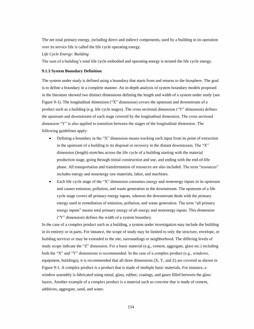
154
The net total primary energy, including direct and indirect components, used by a building in its operation
over its service life is called the life cycle operating energy.
Life Cycle Energy: Building
The sum of a building’s total life cycle embodied and operating energy is termed the life cycle energy.
9.1.3 System Boundary Definition
The system under study is defined using a boundary that starts from and returns to the biosphere. The goal
is to define a boundary in a complete manner. An in-depth analysis of system boundary models proposed
in the literature showed two distinct dimensions defining the length and width of a system under study (see
Figure 9-1). The longitudinal dimension (“X” dimension) covers the upstream and downstream of a
product such as a building (e.g. life cycle stages). The cross sectional dimension (“Y” dimension) defines
the upstream and downstream of each stage covered by the longitudinal dimension. The cross sectional
dimension “Y” is also applied to transition between the stages of the longitudinal dimension. The
following guidelines apply:
Defining a boundary in the “X” dimension means tracking each input from its point of extraction
in the upstream of a building to its disposal or recovery in the distant downstream. The “X”
dimension (length) stretches across the life cycle of a building starting with the material
production stage, going through initial construction and use, and ending with the end-of-life
phase. All transportation and transformation of resources are also included. The term “resources”
includes energy and nonenergy raw materials, labor, and machines.
Each life cycle stage of the “X” dimension consumes energy and nonenergy inputs in its upstream
and causes emission, pollution, and waste generation in the downstream. The upstream of a life
cycle stage covers all primary energy inputs, whereas the downstream deals with the primary
energy used in remediation of emission, pollution, and waste generation. The term “all primary
energy inputs” means total primary energy of all energy and nonenergy inputs. This dimension
(“Y” dimension) defines the width of a system boundary.
In the case of a complex product such as a building, a system under investigation may include the building
in its entirety or in parts. For instance, the scope of study may be limited to only the structure, envelope, or
building services or may be extended to the site, surroundings or neighborhood. The differing levels of
study scope indicate the “Z” dimension. For a basic material (e.g., cement, aggregate, glass etc.) including
both the “X” and “Y” dimensions is recommended. In the case of a complex product (e.g., windows,
equipment, buildings), it is recommended that all three dimensions (X, Y, and Z) are covered as shown in
Figure 9-1. A complex product is a product that is made of multiple basic materials. For instance, a
window assembly is fabricated using metal, glass, rubber, coatings, and gases filled between the glass
layers. Another example of a complex product is a material such as concrete that is made of cement,
additives, aggregate, sand, and water.
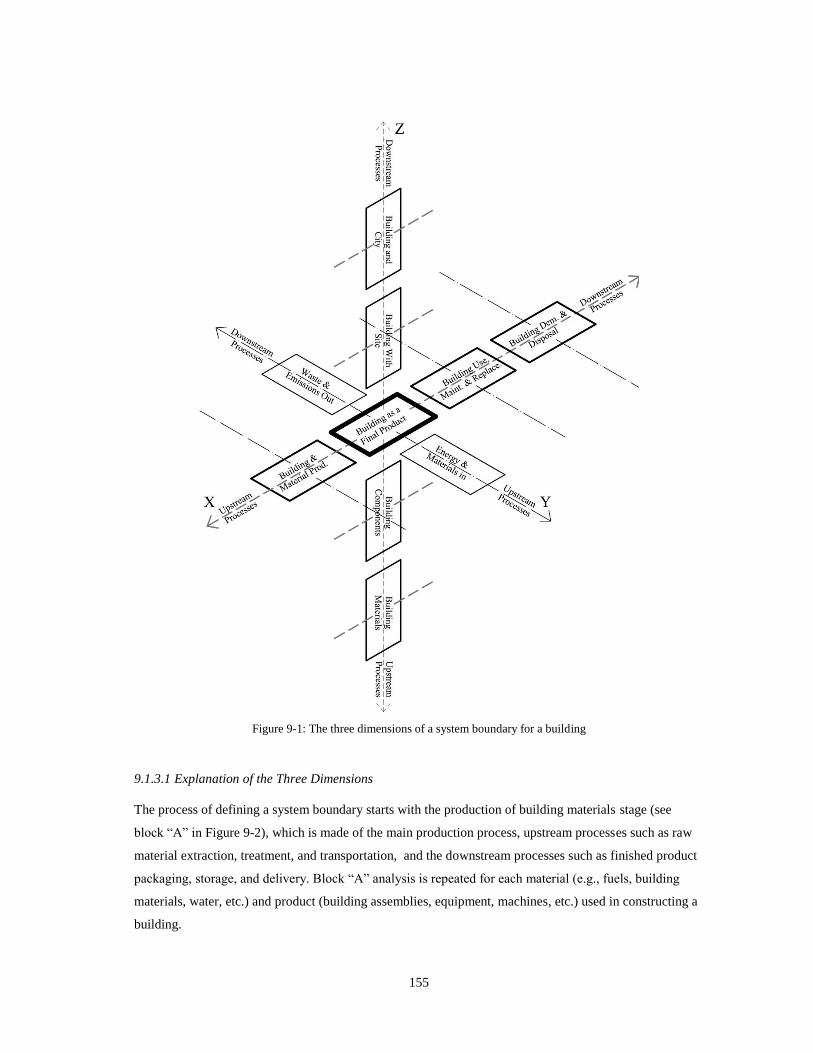
155
Figure 9-1: The three dimensions of a system boundary for a building
9.1.3.1 Explanation of the Three Dimensions
The process of defining a system boundary starts with the production of building materials stage (see
block “A” in Figure 9-2), which is made of the main production process, upstream processes such as raw
material extraction, treatment, and transportation, and the downstream processes such as finished product
packaging, storage, and delivery. Block “A” analysis is repeated for each material (e.g., fuels, building
materials, water, etc.) and product (building assemblies, equipment, machines, etc.) used in constructing a
building.
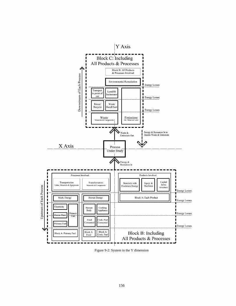
156
Figure 9-2: System in the Y dimension
157
Each block “A” analysis is divided into block “B” and “C” analysis defining the input and output side of
“Y” dimension as shown in Figure 9-2. The input side (block “B”) determines the products and processes
entering each life cycle stage including the transitional stages. The product category consists of raw
materials (including feedstock energy), equipment and machines, and capital infrastructure (e.g.,
automobiles, software, temporary or permanent structures) that are fed into each life cycle stage. For each
item involved in the product input category, the block “A” analysis is done.
The process category represents the transformation or transportation of resources such as material, labor,
and equipment. Each input and output side incorporates mechanical as well as human energy use including
losses due to acquisition (primary fuel extraction or electricity generation), storage, and supply
(transmission and distribution of primary or electrical energy) of energy sources. The losses due to
efficiency of equipment and the productivity of human labor are also accounted for. Block “A” analysis is
repeated for each primary fuel used by machines and each food item consumed by labor. The output side
(block “C”) covers the consumption of resources and energy in the remediation of the environmental
consequences of resource use (input side). Similar to block “B,” each item in the product and process
category is tied back to block “A” analysis. Hence, we can visualize that the system boundary starts with
block “A” analysis, covers blocks “B” and “C,” and finally returns to block “A” analysis at a micro level.
This seems an unending process with each block “A” analysis getting relatively insignificant (in terms of
its relative impact on the product under study) than the earlier one.
Each life cycle stage of a building incorporates blocks “B” and “C” as shown in Figure 9-3, which
illustrates a building’s system boundary comprehensively. As indicated in Figure 9-3, transition from one
stage to another includes each activity of transportation, loading and unloading, temporary storage, etc.
The block “B” and “C” calculations for all products (cranes, trucks, loaders, dumpers, etc.) and processes
(transportation, loading, and unloading) involved in transitional stages are done. Two types of recycling or
reuse of resources are considered: open or closed loop. Resources may also be recovered from combustion
of products that contained feedstock energy (e.g. wood, plastic and other petrochemical products). The
open loop recycling includes recycling and reuse between the life cycle stages or between the various
industry sectors. The closed loop includes reuse or recycling within a life cycle stage or an industry sector.
9.1.4 Embodied Energy: Data Quality
The data utilized in the embodied energy calculation are of two types, the energy and nonenergy inputs.
Two aspects of data used in embodied energy calculation are paramount. First, the data are complete with
respect to the system boundary defined. Second, they are representative of the study with respect to the
location and time.
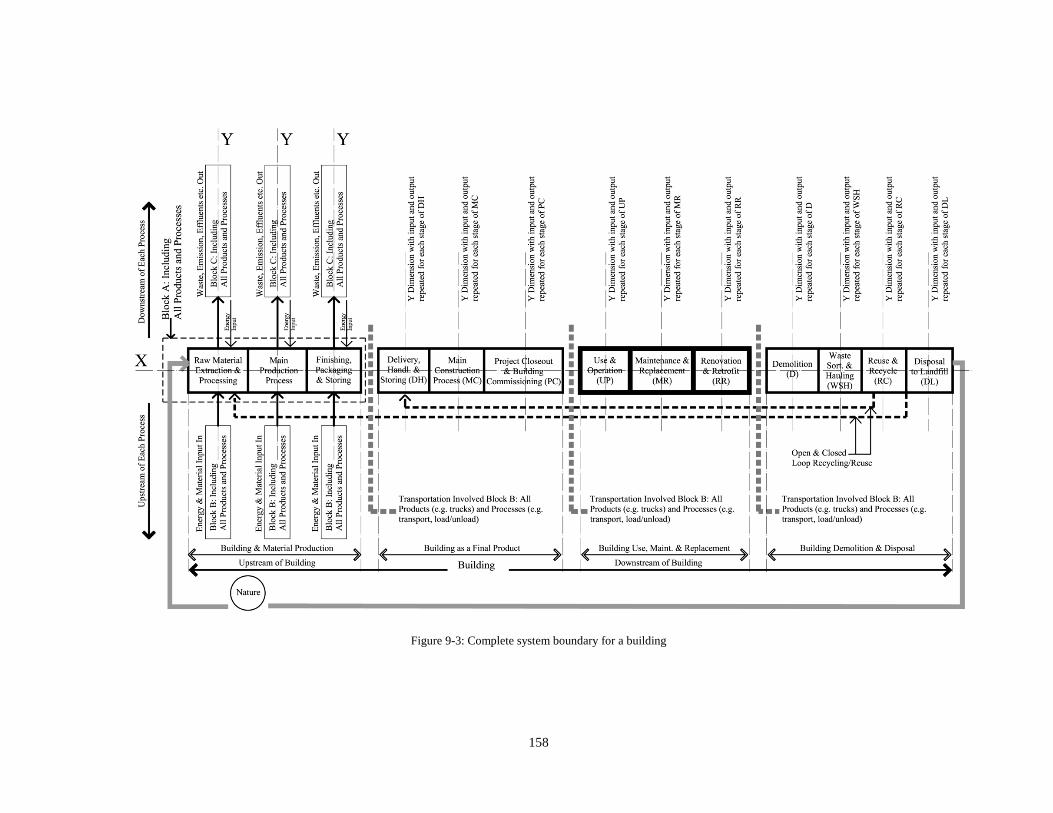
158
Figure 9-3: Complete system boundary for a building

159
9.1.4.1 Data Completeness
The completeness relates to the purpose the data serve in embodied energy analysis. For instance, if
process-based energy intensities are used to replace the direct energy components of an input-output
analysis, they should completely cover all relevant direct inputs. Before incorporating primary data in the
calculation, it is important to apply a calculation method that does not result in incomplete values. If
secondary data are used, it is important to verify their completeness. If the data is found to be incomplete,
it is recommended that necessary adjustments are made to attain completeness.
9.1.4.2 Data Representativeness
The representativeness of data is measured with respect to geographic location, time, and technology. If
primary data are calculated, their representativeness needs to be verified. For instance, data are from the
same region and year as the study, and data represent the technology of manufacture and construction in
terms of resource use. If for any reason old data are used, adjustments are required to convert them to the
current time. If no adjustments can be made, a study for the old time can be performed. However, in such a
case, all other data should also come from the same time period. When using data from a region other than
the study, adjustments are needed based upon the socio-economic and technological aspects.
The technology of manufacture and construction differs with the location. In addition, economic systems
and policies are also different within and across geographic boundaries. Sourcing data from a non-
representative region can produce erroneous results. Even within the same geographic region, if two
manufacturing units apply different technology, their energy intensities are not comparable, and hence,
cannot be substituted for each other. The third aspect relates to the temporal representation of data. If old
data are used, they may not demonstrate the time of the study accurately.
9.1.4.3 Secondary Data
Secondary data can be used if the information about how the data were originally derived is available.
Using data from a source that lacked transparency can seriously hamper the reliability of the energy
results. In addition to transparency, completeness and representativeness of secondary data are also needs
to be verified.
9.1.5 Embodied Energy: Calculation Method
The most commonly used method for embodied energy calculation is the process-based approach.
However, incompleteness due to the truncation of the system boundary is a major issue with this method.
The input-output-based methods are regarded as complete but their results, in most cases, are not specific
to the product under study. Looking at the system boundary model proposed in Section 9.1.3, an input-
output analysis seems the only approach to account for all indirect inputs. The chances that the
incompleteness of a process-based analysis would be improved to an extent that all indirect inputs are

160
counted are rare. In the view of current research, it can be expected that the specificity of an input-output-
based method would improve significantly over time.
An input-output-based hybrid method is appropriate to conduct the embodied energy calculation. The
process data on energy inputs can be collected and inserted into the input-output model to improve its
reliability. The following guidelines apply to an input-output-based hybrid approach:
Avoiding the use of energy and product prices is recommended, as it would improve the
reliability of the method. If possible, replacing direct requirement coefficients of energy use by
process data can avoid relying on energy prices, which vary across industry sectors and
geographic boundaries. In such a case, the direct energy requirement coefficients are calculated
directly in energy units.
Ensure that the inputs such as human energy and capital investment that are not covered in a
conventional input-output model are quantified and added to the economic model.
If disaggregated data on main inputs and outputs of commodities are available, the process of
sector disaggregation is a recommended way to make the results of an input-output-based method
more study specific.
There are multiple chances of double counting due to the way economic input-output accounts
are prepared. One approach used to avoid the double counting of energy is keeping all energy and
nonenergy inputs to zero and multiplying energy intensities with Primary Energy Factors (PEFs)
by fuel. There are sectors such as wholesale and retail trades, which buy energy goods and sell
them for a profit. However, when their energy intensity is quantified based on how much they
bought from the energy providing sectors, the results may be inaccurate because most of the
energy purchased was not consumed but traded.
When using PEFs, the assumption is that the PEFs take into account all indirect energy inputs
consumed by an energy providing sector. Therefore, it is important to calculate PEF for each
energy source in a complete manner by covering all direct and indirect inputs. An input-output-
based hybrid approach is appropriate for calculating the PEFs.
If all energy sources used in an economy are averaged into one energy source for the purpose of
calculating the embodied energy, its relevance to environmental issues is lost. Embodied energy
results by fuel type can be used to further quantify other environmental impacts such as carbon
emission and pollution.
Once the embodied energy intensities of industry sectors are calculated, product prices are used to
convert the energy intensities to embodied energy values per unit of mass or volume. If suitable
data are readily available, using the production quantity of a finished product and the total
embodied energy of the sector manufacturing the product, embodied energy per unit of mass or
161
volume can be calculated without using the price of the product. Using product prices for
converting energy intensities to energy units poses serious problems, as product prices also vary
and may be underestimated or overestimated. For instance, iron and steel mills sector not only
manufactures virgin steel but also produces a wide range of structural shapes each of which has
quite different prices. One way to avoid this is collecting data on total production of the product
in physical quantities. The calculated embodied energy values then can be multiplied by the
monetary sectorial output to obtain total embodied energy of the entire industry sector. This value
if divided by the total embodied energy would give embodied energy per unit of mass or volume.
9.1.6 Embodied Energy: Reporting
It is recommended that the reporting of the embodied energy process and results is done in a transparent
manner so that the reader can make informed decisions about analyzing or applying the study with or
without modifications. The following information must be supplied in order to attain a reasonable degree
of transparency:
System boundary: A boundary defining the extent of the study is graphically supplied and
explained in the text in detail. Each input, major or minor, is reported if included or excluded
from the system. Any recovery of resources is mentioned in the text. As mentioned in Section
8.1.3, a complete coverage of the system boundary is recommended. If the product under study is
a complex product such as a building, a detailed account of its and its constituent materials’
service life is given. Factors such as a waste factor and replacement factor, if used in the
calculation, are listed clearly by each material and assembly. Any schedule of maintenance or
renovation, if applied, needs to be explained while reporting the system boundary.
Calculation method: The method applied for the calculation is explained step by step stating and
explaining each variable. If any modification is done to an established method, it needs
explanation so that a reader can evaluate the applicability of the modified method. All major
assumptions regarding energy and nonenergy inputs and calculation process are listed. It is also
recommended that the approach to evaluate the study results is explained clearly.
Data sources: Any primary or secondary source referred in the study needs to be listed along with
a way to approach them if needed. Three types of information are included in data source
reporting: date, geographic location, and the details of the publishing organization or agency. If
any modification is done to the sourced data to improve its representativeness, it needs detailed
explanation.
Study results: The embodied energy results are presented in primary energy units only. If
secondary energy units are used, a factor to convert them into primary units is supplied and

162
explained. Embodied energy results are reported collectively and also by each fuel or energy
source used in the region.
Case study description: In the case of a research conducting case studies of materials or products,
a detailed description of their physical, spatial, and environmental characteristics is
recommended. For instance, if the study object is a building, information about its construction
(at a minimum, structural frame, envelope, and interiors), design (representative floor plans and
sections), and surroundings (site, climate, and socio-economic conditions) is mentioned briefly in
the report.
9.2 EMBODIED ENERGY OF STUDY MATERIALS
This chapter provides the results of the embodied energy calculation performed for the study materials.
The calculated values are presented as energy intensities per unit of monetary output and also as embodied
energy per unit of mass. The results are also reported by each energy source so that the share of each in the
total carbon emission can be analyzed at a later date. Reporting of results by each stage is also provided to
demonstrate how energy intensities get smaller with each stage in the upstream. Here, upstream stages
indicate the subcomponents of a material. For instance, the use of cement in the production of concrete is
stage I input to concrete. Similarly the use of limestone in manufacturing cement is the stage II input to
concrete production and so on. It is also important to analyze the share of direct and indirect components
in the total embodied energy. For some materials, the direct energy could be significantly less than the
indirect fraction of the total embodied energy. As the calculations were performed in steps indicating
gradual improvements, the results are also presented by each step to observe the impact on embodied
energy.
9.2.1 Embodied Energy of Study Materials
Table 9-1 provides the values of embodied energy calculated for each study material. The values are listed
for each calculation approach. The first column lists embodied energy calculated using a basic input-
output approach in which the total energy coefficients were calculated by dividing the total requirements
with average energy prices. In the second approach, in order to avoid the use of average energy prices,
process data of energy use were inserted into the input-output model. The human and capital energy were
added in the next approach. Finally, some sectors were disaggregated to quantify the material specific
embodied energy for materials such as wood, plywood, brick, clay tiles, vitrified clay pipes, gypsum
building products, lime, steel, and primary aluminum. Materials such as wood lumbers are manufactured
by a sector that is also engaged in wood preservation activities, and hence, embodied energy specific to
wood lumber production should be calculated separately. The embodied energy of wood lumber changed
slightly from 2.7 to 2.8 kBtu/lb after the sector disaggregation. However, in the case of hardwood plywood
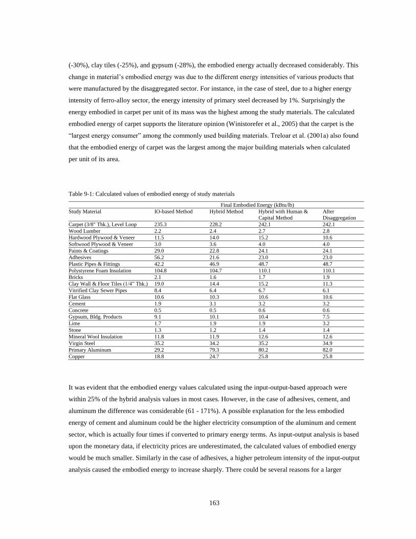
163
(-30%), clay tiles (-25%), and gypsum (-28%), the embodied energy actually decreased considerably. This
change in material’s embodied energy was due to the different energy intensities of various products that
were manufactured by the disaggregated sector. For instance, in the case of steel, due to a higher energy
intensity of ferro-alloy sector, the energy intensity of primary steel decreased by 1%. Surprisingly the
energy embodied in carpet per unit of its mass was the highest among the study materials. The calculated
embodied energy of carpet supports the literature opinion (Winistorefer et al., 2005) that the carpet is the
“largest energy consumer” among the commonly used building materials. Treloar et al. (2001a) also found
that the embodied energy of carpet was the largest among the major building materials when calculated
per unit of its area.
Table 9-1: Calculated values of embodied energy of study materials
Final Embodied Energy (kBtu/lb)
Study Material IO-based Method Hybrid Method Hybrid with Human &
Capital Method
After
Disaggregation
Carpet (3/8" Thk.), Level Loop 235.3 228.2 242.1 242.1
Wood Lumber 2.2 2.4 2.7 2.8
Hardwood Plywood & Veneer 11.5 14.0 15.2 10.6
Softwood Plywood & Veneer 3.0 3.6 4.0 4.0
Paints & Coatings 29.0 22.8 24.1 24.1
Adhesives 56.2 21.6 23.0 23.0
Plastic Pipes & Fittings 42.2 46.9 48.7 48.7
Polystyrene Foam Insulation 104.8 104.7 110.1 110.1
Bricks 2.1 1.6 1.7 1.9
Clay Wall & Floor Tiles (1/4” Thk.) 19.0 14.4 15.2 11.3
Vitrified Clay Sewer Pipes 8.4 6.4 6.7 6.1
Flat Glass 10.6 10.3 10.6 10.6
Cement 1.9 3.1 3.2 3.2
Concrete 0.5 0.5 0.6 0.6
Gypsum, Bldg. Products 9.1 10.1 10.4 7.5
Lime 1.7 1.9 1.9 3.2
Stone 1.3 1.2 1.4 1.4
Mineral Wool Insulation 11.8 11.9 12.6 12.6
Virgin Steel 35.2 34.2 35.2 34.9
Primary Aluminum 29.2 79.3 80.2 82.0
Copper 18.8 24.7 25.8 25.8
It was evident that the embodied energy values calculated using the input-output-based approach were
within 25% of the hybrid analysis values in most cases. However, in the case of adhesives, cement, and
aluminum the difference was considerable (61 - 171%). A possible explanation for the less embodied
energy of cement and aluminum could be the higher electricity consumption of the aluminum and cement
sector, which is actually four times if converted to primary energy terms. As input-output analysis is based
upon the monetary data, if electricity prices are underestimated, the calculated values of embodied energy
would be much smaller. Similarly in the case of adhesives, a higher petroleum intensity of the input-output
analysis caused the embodied energy to increase sharply. There could be several reasons for a larger

164
embodied energy of chemical products such as adhesives. The chances of double counting and a large
share of feedstock energy use are among them. Based on these results, it can be concluded that the results
of an input-output-based analysis are quite different than the other hybrid methods. Although the increase
in embodied energy due to the inclusion of human and capital inputs was within 10% for most materials,
in the case of wood lumber and stone, it actually increased by 11 - 17%. The least change occurred in the
case of aluminum, where embodied energy increased by just one percent as a result of human and capital
energy inclusion.
9.2.2 Energy Intensities by Energy Source
Figure 9-4, Figure 9-5, and Figure 9-6 demonstrate the energy intensities in MBtu/$ output of the study
material sector by energy source calculated using the three approaches. It can be seen that the fuel
intensities were quite different in the input-output-based and input-output-based hybrid approaches. In the
input-output-based approach, the electricity use was mostly within 0.005 MBtu/$ except for the aluminum
production. However, in the hybrid approaches, it increased to a range of 0.007 - 0.08 MBtu/$. The most
electricity-intensive sector was the primary aluminum production, which consumed 0.08 MBtu of energy
per dollar of its output. Other sectors producing materials such as cement (0.026 MBtu/$), gypsum (0.012
MBtu/$), and lime (0.012 MBtu/$) also consumed considerable electricity. The cement manufacturing
sector was the most coal-intensive sector. Other sectors producing steel, gypsum, and lime also consumed
coal in relatively large quantities per dollar of their outputs. Interestingly, the aluminum and plastic
industries were among the most petroleum-consuming industries.
The effect of sectorial disaggregation is clearly visible in Figure 9-6 . The seemingly flat energy use of
gypsum, lime, and clay product manufacturing as seen in Figure 9-5 , disappeared in Figure 9-6. The
significance of reporting energy use by energy source is that one can identify sectors that are critical to
combating the increased levels of carbon emissions. Sectors producing aluminum, steel, and cement
consume considerably higher quantities of electricity and coal energy, the key contributors to global
carbon emissions.
Figure 9-7 shows the share of each fuel in the total energy used by sectors producing the study materials.
Figure 9-7 only presents the results of the input-output-based hybrid analysis with human and capital
inputs after disaggregation. It can be observed that nearly 25% of the total energy requirements of all
sectors came from the electricity and coal supply. Materials such as aluminum, steel, and cement used
extensively in building construction, came from manufacturing sectors that were the largest consumers of
electricity and coal (>50% of the total energy use collectively). The fraction of human energy in the total
embodied energy ranged from 0.7-9.3%, whereas it was within 1.2 - 5.2% for the capital energy. The
calculated energy intensities per dollar of sectorial output by each energy source are listed in Table A1-16,
Table A1-17, Table A1-18, and Table A1-19 in Appendix A1.
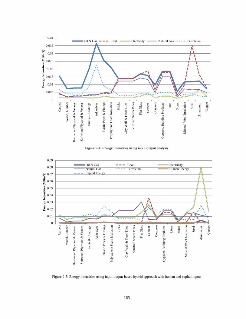
165
Figure 9-4: Energy intensities using input-output analysis
Figure 9-5: Energy intensities using input-output-based hybrid approach with human and capital inputs
0
0.005
0.01
0.015
0.02
0.025
0.03
0.035
0.04
Car
pet
s
Woo
d, L
um
ber
Har
dw
ood P
lyw
oo
d &
Ven
eer
Soft
wo
od P
lyw
oo
d &
Ven
eer
Pai
nts
& C
oat
ings
Adh
esiv
es
Pla
stic
Pip
es &
Fit
tin
gs
Poly
styre
ne
Foam
In
sula
tion
Bri
cks
Cla
y W
all
& F
loor
Til
es
Vit
rifi
ed S
ewer
Pip
es
Fla
t G
lass
Cem
ent
Co
ncr
ete
Gyp
sum
, B
uil
din
g P
rodu
cts
Lim
e
Sto
ne
Min
eral
Wool
Insu
lati
on
Ste
el
Alu
min
um
Co
pper
En
erg
y I
nte
nsi
ties
(MB
tu/$
) Oil & Gas Coal Electricity Natural Gas Petroleum
0
0.01
0.02
0.03
0.04
0.05
0.06
0.07
0.08
0.09
Car
pet
s
Woo
d, L
um
ber
Har
dw
ood P
lyw
oo
d &
Ven
eer
Soft
wo
od P
lyw
oo
d &
Ven
eer
Pai
nts
& C
oat
ings
Adh
esiv
es
Pla
stic
Pip
es &
Fit
tin
gs
Poly
styre
ne
Foam
In
sula
tion
Bri
cks
Cla
y W
all
& F
loor
Til
es
Vit
rifi
ed S
ewer
Pip
es
Fla
t G
lass
Cem
ent
Co
ncr
ete
Gyp
sum
, B
uil
din
g P
rodu
cts
Lim
e
Sto
ne
Min
eral
Wool
Insu
lati
on
Ste
el
Alu
min
um
Co
pper
En
erg
y I
nte
nsi
ties
(MB
tu/$
)
Oil & Gas Coal Electricity
Natural Gas Petroleum Human Energy
Capital Energy
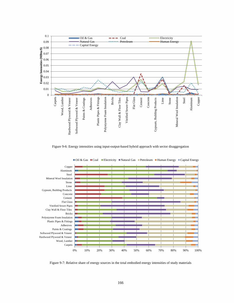
166
Figure 9-6: Energy intensities using input-output-based hybrid approach with sector disaggregation
Figure 9-7: Relative share of energy sources in the total embodied energy intensities of study materials
0
0.01
0.02
0.03
0.04
0.05
0.06
0.07
0.08
0.09
0.1
Car
pet
s
Woo
d, L
um
ber
Har
dw
ood P
lyw
oo
d &
Ven
eer
Soft
wo
od P
lyw
oo
d &
Ven
eer
Pai
nts
& C
oat
ings
Adh
esiv
es
Pla
stic
Pip
es &
Fit
tin
gs
Poly
styre
ne
Foam
In
sula
tion
Bri
cks
Cla
y W
all
& F
loor
Til
es
Vit
rifi
ed S
ewer
Pip
es
Fla
t G
lass
Cem
ent
Co
ncr
ete
Gyp
sum
, B
uil
din
g P
rodu
cts
Lim
e
Sto
ne
Min
eral
Wool
Insu
lati
on
Ste
el
Alu
min
um
Co
pper
En
erg
y I
nte
nsi
ties
(MB
tu/$
) Oil & Gas Coal Electricity
Natural Gas Petroleum Human Energy
Capital Energy
0% 10% 20% 30% 40% 50% 60% 70% 80% 90% 100%
Carpets
Wood, Lumber
Hardwood Plywood & Veneer
Softwood Plywood & Veneer
Paints & Coatings
Adhesives
Plastic Pipes & Fittings
Polystyrene Foam Insulation
Bricks
Clay Wall & Floor Tiles
Vitrified Sewer Pipes
Flat Glass
Cement
Concrete
Gypsum, Building Products
Lime
Stone
Mineral Wool Insulation
Steel
Aluminum
Copper
Oil & Gas Coal Electricity Natural Gas Petroleum Human Energy Capital Energy
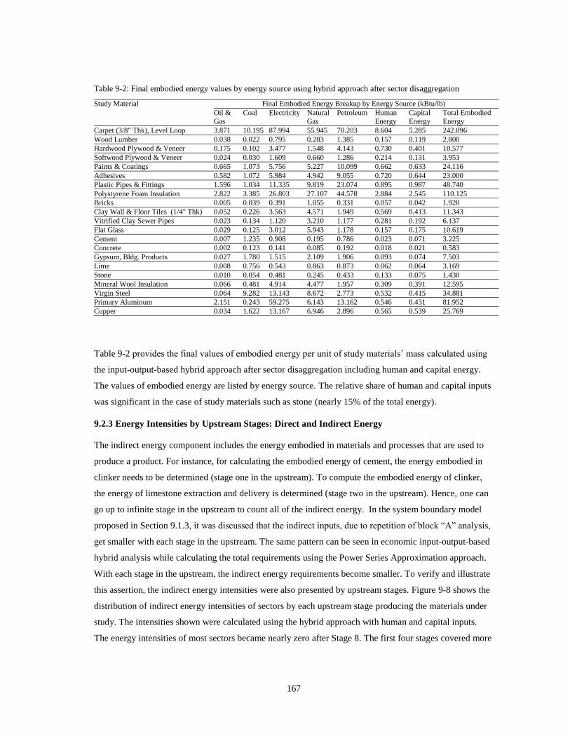
167
Table 9-2: Final embodied energy values by energy source using hybrid approach after sector disaggregation
Study Material Final Embodied Energy Breakup by Energy Source (kBtu/lb)
Oil &
Gas
Coal Electricity Natural
Gas
Petroleum Human
Energy
Capital
Energy
Total Embodied
Energy
Carpet (3/8" Thk), Level Loop 3.871 10.195 87.994 55.945 70.203 8.604 5.285 242.096
Wood Lumber 0.038 0.022 0.795 0.283 1.385 0.157 0.119 2.800
Hardwood Plywood & Veneer 0.175 0.102 3.477 1.548 4.143 0.730 0.401 10.577
Softwood Plywood & Veneer 0.024 0.030 1.609 0.660 1.286 0.214 0.131 3.953
Paints & Coatings 0.665 1.073 5.756 5.227 10.099 0.662 0.633 24.116
Adhesives 0.582 1.072 5.984 4.942 9.055 0.720 0.644 23.000
Plastic Pipes & Fittings 1.596 1.034 11.335 9.819 23.074 0.895 0.987 48.740
Polystyrene Foam Insulation 2.822 3.385 26.803 27.107 44.578 2.884 2.545 110.125
Bricks 0.005 0.039 0.391 1.055 0.331 0.057 0.042 1.920
Clay Wall & Floor Tiles (1/4" Thk) 0.052 0.226 3.563 4.571 1.949 0.569 0.413 11.343
Vitrified Clay Sewer Pipes 0.023 0.134 1.120 3.210 1.177 0.281 0.192 6.137
Flat Glass 0.029 0.125 3.012 5.943 1.178 0.157 0.175 10.619
Cement 0.007 1.235 0.908 0.195 0.786 0.023 0.071 3.225
Concrete 0.002 0.123 0.141 0.085 0.192 0.018 0.021 0.583
Gypsum, Bldg. Products 0.027 1.780 1.515 2.109 1.906 0.093 0.074 7.503
Lime 0.008 0.756 0.543 0.863 0.873 0.062 0.064 3.169
Stone 0.010 0.054 0.481 0.245 0.433 0.133 0.075 1.430
Mineral Wool Insulation 0.066 0.481 4.914 4.477 1.957 0.309 0.391 12.595
Virgin Steel 0.064 9.282 13.143 8.672 2.773 0.532 0.415 34.881
Primary Aluminum 2.151 0.243 59.275 6.143 13.162 0.546 0.431 81.952
Copper 0.034 1.622 13.167 6.946 2.896 0.565 0.539 25.769
Table 9-2 provides the final values of embodied energy per unit of study materials’ mass calculated using
the input-output-based hybrid approach after sector disaggregation including human and capital energy.
The values of embodied energy are listed by energy source. The relative share of human and capital inputs
was significant in the case of study materials such as stone (nearly 15% of the total energy).
9.2.3 Energy Intensities by Upstream Stages: Direct and Indirect Energy
The indirect energy component includes the energy embodied in materials and processes that are used to
produce a product. For instance, for calculating the embodied energy of cement, the energy embodied in
clinker needs to be determined (stage one in the upstream). To compute the embodied energy of clinker,
the energy of limestone extraction and delivery is determined (stage two in the upstream). Hence, one can
go up to infinite stage in the upstream to count all of the indirect energy. In the system boundary model
proposed in Section 9.1.3, it was discussed that the indirect inputs, due to repetition of block “A” analysis,
get smaller with each stage in the upstream. The same pattern can be seen in economic input-output-based
hybrid analysis while calculating the total requirements using the Power Series Approximation approach.
With each stage in the upstream, the indirect energy requirements become smaller. To verify and illustrate
this assertion, the indirect energy intensities were also presented by upstream stages. Figure 9-8 shows the
distribution of indirect energy intensities of sectors by each upstream stage producing the materials under
study. The intensities shown were calculated using the hybrid approach with human and capital inputs.
The energy intensities of most sectors became nearly zero after Stage 8. The first four stages covered more
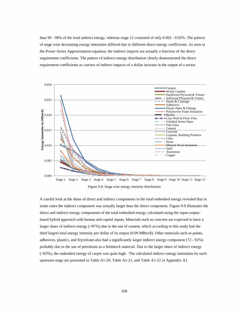
168
than 90 - 98% of the total indirect energy, whereas stage 12 consisted of only 0.002 - 0.02%. The pattern
of stage wise decreasing energy intensities differed due to different direct energy coefficients. As seen in
the Power Series Approximation equation, the indirect impacts are actually a function of the direct
requirement coefficients. The pattern of indirect energy distribution clearly demonstrated the direct
requirement coefficients as carriers of indirect impacts of a dollar increase in the output of a sector.
Figure 9-8: Stage wise energy intensity distribution
A careful look at the share of direct and indirect components in the total embodied energy revealed that in
some cases the indirect component was actually larger than the direct component. Figure 9-9 illustrates the
direct and indirect energy components of the total embodied energy calculated using the input-output-
based hybrid approach with human and capital inputs. Materials such as concrete are expected to have a
larger share of indirect energy (>87%) due to the use of cement, which according to this study had the
third largest total energy intensity per dollar of its output (0.09 MBtu/$). Other materials such as paints,
adhesives, plastics, and Styrofoam also had a significantly larger indirect energy component (72 - 92%)
probably due to the use of petroleum as a feedstock material. Due to the larger share of indirect energy
(>83%), the embodied energy of carpet was quite high. The calculated indirect energy intensities by each
upstream stage are presented in Table A1-20, Table A1-21, and Table A1-22 in Appendix A1.
0.000
0.005
0.010
0.015
0.020
0.025
0.030
Stage 1 Stage 2 Stage 3 Stage 4 Stage 5 Stage 6 Stage 7 Stage 8 Stage 9 Stage 10 Stage 11 Stage 12
En
erg
y I
nte
nsi
ties
in (
Mb
tu/$
)
CarpetsWood, LumberHardwood Plywood & VeneerSoftwood Plywood & VeneerPaints & CoatingsAdhesivesPlastic Pipes & FittingsPolystyrene Foam InsulationBricksClay Wall & Floor TilesVitrified Sewer PipesFlat GlassCementConcreteGypsum, Building ProductsLimeStoneMineral Wool InsulationSteelAluminumCopper
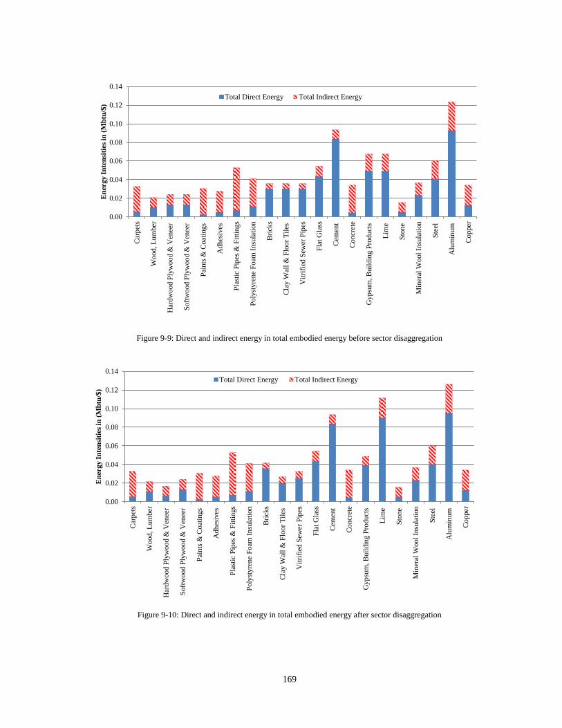
169
Figure 9-9: Direct and indirect energy in total embodied energy before sector disaggregation
Figure 9-10: Direct and indirect energy in total embodied energy after sector disaggregation
0.00
0.02
0.04
0.06
0.08
0.10
0.12
0.14
Car
pet
s
Woo
d, L
um
ber
Har
dw
ood P
lyw
oo
d &
Ven
eer
Soft
wo
od P
lyw
oo
d &
Ven
eer
Pai
nts
& C
oat
ings
Adh
esiv
es
Pla
stic
Pip
es &
Fit
tin
gs
Poly
styre
ne
Foam
In
sula
tion
Bri
cks
Cla
y W
all
& F
loo
r T
iles
Vit
rifi
ed S
ewer
Pip
es
Fla
t G
lass
Cem
ent
Co
ncr
ete
Gyp
sum
, B
uil
din
g P
rodu
cts
Lim
e
Sto
ne
Min
eral
Wool
Insu
lati
on
Ste
el
Alu
min
um
Co
pper
En
erg
y I
nte
nsi
ties
in (
Mb
tu/$
) Total Direct Energy Total Indirect Energy
0.00
0.02
0.04
0.06
0.08
0.10
0.12
0.14
Car
pet
s
Woo
d, L
um
ber
Har
dw
ood P
lyw
oo
d &
Ven
eer
Soft
wo
od P
lyw
oo
d &
Ven
eer
Pai
nts
& C
oat
ings
Adh
esiv
es
Pla
stic
Pip
es &
Fit
tin
gs
Poly
styre
ne
Foam
In
sula
tion
Bri
cks
Cla
y W
all
& F
loo
r T
iles
Vit
rifi
ed S
ewer
Pip
es
Fla
t G
lass
Cem
ent
Co
ncr
ete
Gyp
sum
, B
uil
din
g P
rodu
cts
Lim
e
Sto
ne
Min
eral
Wool
Insu
lati
on
Ste
el
Alu
min
um
Co
pper
En
erg
y I
nte
nsi
ties
in (
Mb
tu/$
)
Total Direct Energy Total Indirect Energy
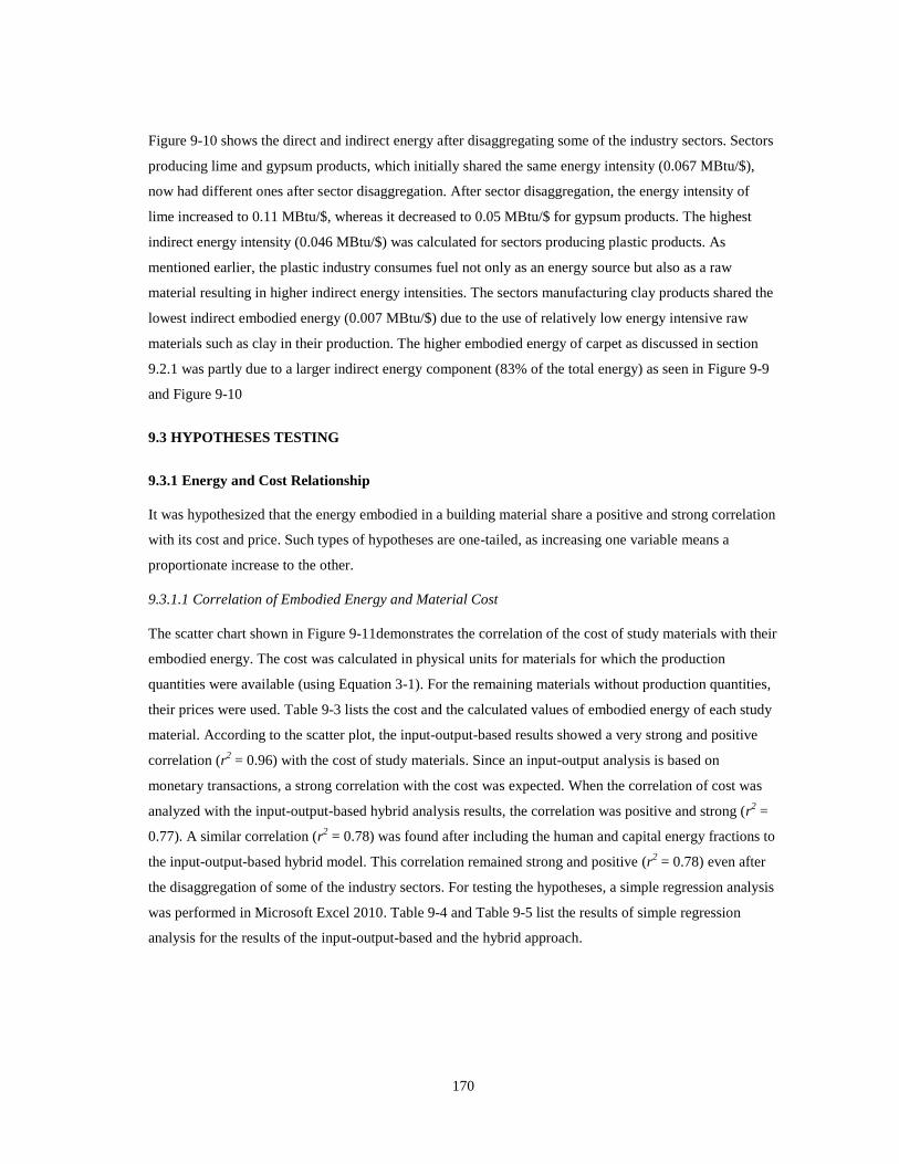
170
Figure 9-10 shows the direct and indirect energy after disaggregating some of the industry sectors. Sectors
producing lime and gypsum products, which initially shared the same energy intensity (0.067 MBtu/$),
now had different ones after sector disaggregation. After sector disaggregation, the energy intensity of
lime increased to 0.11 MBtu/$, whereas it decreased to 0.05 MBtu/$ for gypsum products. The highest
indirect energy intensity (0.046 MBtu/$) was calculated for sectors producing plastic products. As
mentioned earlier, the plastic industry consumes fuel not only as an energy source but also as a raw
material resulting in higher indirect energy intensities. The sectors manufacturing clay products shared the
lowest indirect embodied energy (0.007 MBtu/$) due to the use of relatively low energy intensive raw
materials such as clay in their production. The higher embodied energy of carpet as discussed in section
9.2.1 was partly due to a larger indirect energy component (83% of the total energy) as seen in Figure 9-9
and Figure 9-10
9.3 HYPOTHESES TESTING
9.3.1 Energy and Cost Relationship
It was hypothesized that the energy embodied in a building material share a positive and strong correlation
with its cost and price. Such types of hypotheses are one-tailed, as increasing one variable means a
proportionate increase to the other.
9.3.1.1 Correlation of Embodied Energy and Material Cost
The scatter chart shown in Figure 9-11demonstrates the correlation of the cost of study materials with their
embodied energy. The cost was calculated in physical units for materials for which the production
quantities were available (using Equation 3-1). For the remaining materials without production quantities,
their prices were used. Table 9-3 lists the cost and the calculated values of embodied energy of each study
material. According to the scatter plot, the input-output-based results showed a very strong and positive
correlation (r2 = 0.96) with the cost of study materials. Since an input-output analysis is based on
monetary transactions, a strong correlation with the cost was expected. When the correlation of cost was
analyzed with the input-output-based hybrid analysis results, the correlation was positive and strong (r2 =
0.77). A similar correlation (r2 = 0.78) was found after including the human and capital energy fractions to
the input-output-based hybrid model. This correlation remained strong and positive (r2 = 0.78) even after
the disaggregation of some of the industry sectors. For testing the hypotheses, a simple regression analysis
was performed in Microsoft Excel 2010. Table 9-4 and Table 9-5 list the results of simple regression
analysis for the results of the input-output-based and the hybrid approach.
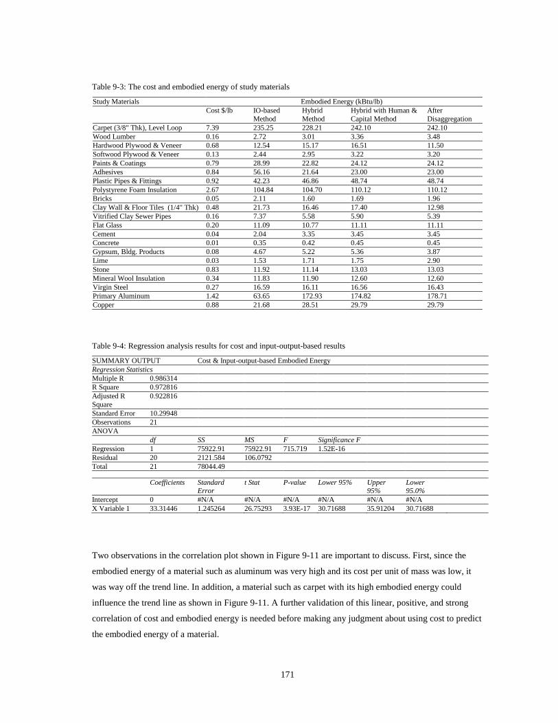
171
Table 9-3: The cost and embodied energy of study materials
Study Materials Embodied Energy (kBtu/lb)
Cost $/lb IO-based
Method
Hybrid
Method
Hybrid with Human &
Capital Method
After
Disaggregation
Carpet (3/8" Thk), Level Loop 7.39 235.25 228.21 242.10 242.10
Wood Lumber 0.16 2.72 3.01 3.36 3.48
Hardwood Plywood & Veneer 0.68 12.54 15.17 16.51 11.50
Softwood Plywood & Veneer 0.13 2.44 2.95 3.22 3.20
Paints & Coatings 0.79 28.99 22.82 24.12 24.12
Adhesives 0.84 56.16 21.64 23.00 23.00
Plastic Pipes & Fittings 0.92 42.23 46.86 48.74 48.74
Polystyrene Foam Insulation 2.67 104.84 104.70 110.12 110.12
Bricks 0.05 2.11 1.60 1.69 1.96
Clay Wall & Floor Tiles (1/4" Thk) 0.48 21.73 16.46 17.40 12.98
Vitrified Clay Sewer Pipes 0.16 7.37 5.58 5.90 5.39
Flat Glass 0.20 11.09 10.77 11.11 11.11
Cement 0.04 2.04 3.35 3.45 3.45
Concrete 0.01 0.35 0.42 0.45 0.45
Gypsum, Bldg. Products 0.08 4.67 5.22 5.36 3.87
Lime 0.03 1.53 1.71 1.75 2.90
Stone 0.83 11.92 11.14 13.03 13.03
Mineral Wool Insulation 0.34 11.83 11.90 12.60 12.60
Virgin Steel 0.27 16.59 16.11 16.56 16.43
Primary Aluminum 1.42 63.65 172.93 174.82 178.71
Copper 0.88 21.68 28.51 29.79 29.79
Table 9-4: Regression analysis results for cost and input-output-based results
SUMMARY OUTPUT Cost & Input-output-based Embodied Energy
Regression Statistics
Multiple R 0.986314
R Square 0.972816
Adjusted R
Square
0.922816
Standard Error 10.29948
Observations 21
ANOVA
df SS MS F Significance F
Regression 1 75922.91 75922.91 715.719 1.52E-16
Residual 20 2121.584 106.0792
Total 21 78044.49
Coefficients Standard
Error t Stat P-value Lower 95% Upper
95% Lower 95.0%
Intercept 0 #N/A #N/A #N/A #N/A #N/A #N/A
X Variable 1 33.31446 1.245264 26.75293 3.93E-17 30.71688 35.91204 30.71688
Two observations in the correlation plot shown in Figure 9-11 are important to discuss. First, since the
embodied energy of a material such as aluminum was very high and its cost per unit of mass was low, it
was way off the trend line. In addition, a material such as carpet with its high embodied energy could
influence the trend line as shown in Figure 9-11. A further validation of this linear, positive, and strong
correlation of cost and embodied energy is needed before making any judgment about using cost to predict
the embodied energy of a material.
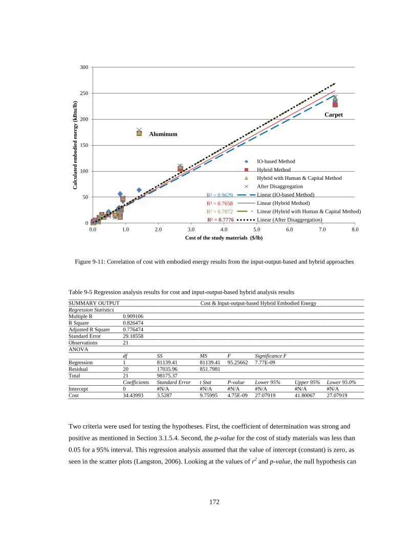
172
Figure 9-11: Correlation of cost with embodied energy results from the input-output-based and hybrid approaches
Table 9-5 Regression analysis results for cost and input-output-based hybrid analysis results
SUMMARY OUTPUT Cost & Input-output-based Hybrid Embodied Energy
Regression Statistics
Multiple R 0.909106
R Square 0.826474
Adjusted R Square 0.776474
Standard Error 29.18558
Observations 21
ANOVA
df SS MS F Significance F
Regression 1 81139.41 81139.41 95.25662 7.77E-09
Residual 20 17035.96 851.7981
Total 21 98175.37
Coefficients Standard Error t Stat P-value Lower 95% Upper 95% Lower 95.0%
Intercept 0 #N/A #N/A #N/A #N/A #N/A #N/A
Cost 34.43993 3.5287 9.75995 4.75E-09 27.07919 41.80067 27.07919
Two criteria were used for testing the hypotheses. First, the coefficient of determination was strong and
positive as mentioned in Section 3.1.5.4. Second, the p-value for the cost of study materials was less than
0.05 for a 95% interval. This regression analysis assumed that the value of intercept (constant) is zero, as
seen in the scatter plots (Langston, 2006). Looking at the values of r2 and p-value, the null hypothesis can
R² = 0.9629
R² = 0.7658
R² = 0.7872
R² = 0.7776 0
50
100
150
200
250
300
0.0 1.0 2.0 3.0 4.0 5.0 6.0 7.0 8.0
Ca
lcu
late
d e
mb
od
ied
en
erg
y (
kB
tu/l
b)
Cost of the study materials ($/lb)
IO-based Method
Hybrid Method
Hybrid with Human & Capital Method
After Disaggregation
Linear (IO-based Method)
Linear (Hybrid Method)
Linear (Hybrid with Human & Capital Method)
Linear (After Disaggregation)
Carpet
Aluminum

173
be rejected in favor of the alternative hypothesis. The same is found true for the embodied energy results
obtained after adding the human and capital inputs and disaggregating the industry sectors. Based on the
results, a strong and positive correlation was found between the cost and the embodied energy of study
materials calculated using an input-output-based hybrid analysis. The regression analysis results can be
seen in Table A1-8 and Table A1-9 in Appendix A1 for other hybrid approaches.
9.3.1.2 Correlation of Embodied Energy and Material Price
To test the second hypothesis, the correlation between the study materials’ price and embodied energy was
evaluated. Table 9-6 provides the materials’ price and embodied energy data. The correlation of the price
of study materials was checked with the energy results of all four approaches (one input-output-based and
three input-output-based hybrid methods). The material prices were plotted on the x-axis, whereas the
embodied energy values on the y-axis. The initial scatter plot, as shown in Figure 9-12, exhibited a very
strong and positive correlation of the study materials’ price and embodied energy. In the case of the results
of input-output-based analysis, the value of r2 was 0.97, which decreased to 0.92 when the hybrid analysis
results were used. After adding the human and capital energy, the correlation remained very strong and
positive (r2= 0.93). The value of r
2 was 0.93 for embodied energy values calculated after disaggregating
the industry sectors.
To test the second hypothesis, a simple regression analysis was performed using Microsoft Excel 2010.
Again, the origin was assumed as zero and the values of r2 and p-value were used to reject or accept the
null hypothesis. The results of regression analysis are shown in Table 9-7 and Table 9-8 for the input-
output-based and input-output-based hybrid embodied energy values. Similar to the cost and embodied
energy correlation, the higher embodied energy of carpet tends to influence the trend line. However, in the
case of material price and embodied energy correlation, the point representing aluminum came close to the
trend line as seen in Figure 9-12. As mentioned earlier, a further validation of this correlation is required in
the future.
The values of r2 were found greater than 0.9 in both the cases indicating a very strong and positive
correlation. In the case of input-output-based hybrid method, the p-value for material prices was less than
0.05 at 95% confidence interval. Hence, observing the value of r2 and p-value, the null hypothesis can be
rejected in favor of the alternative hypothesis. The results of regression analysis for other hybrid
approaches can be seen in Table A1-10 and Table A1-11 in Appendix A1.
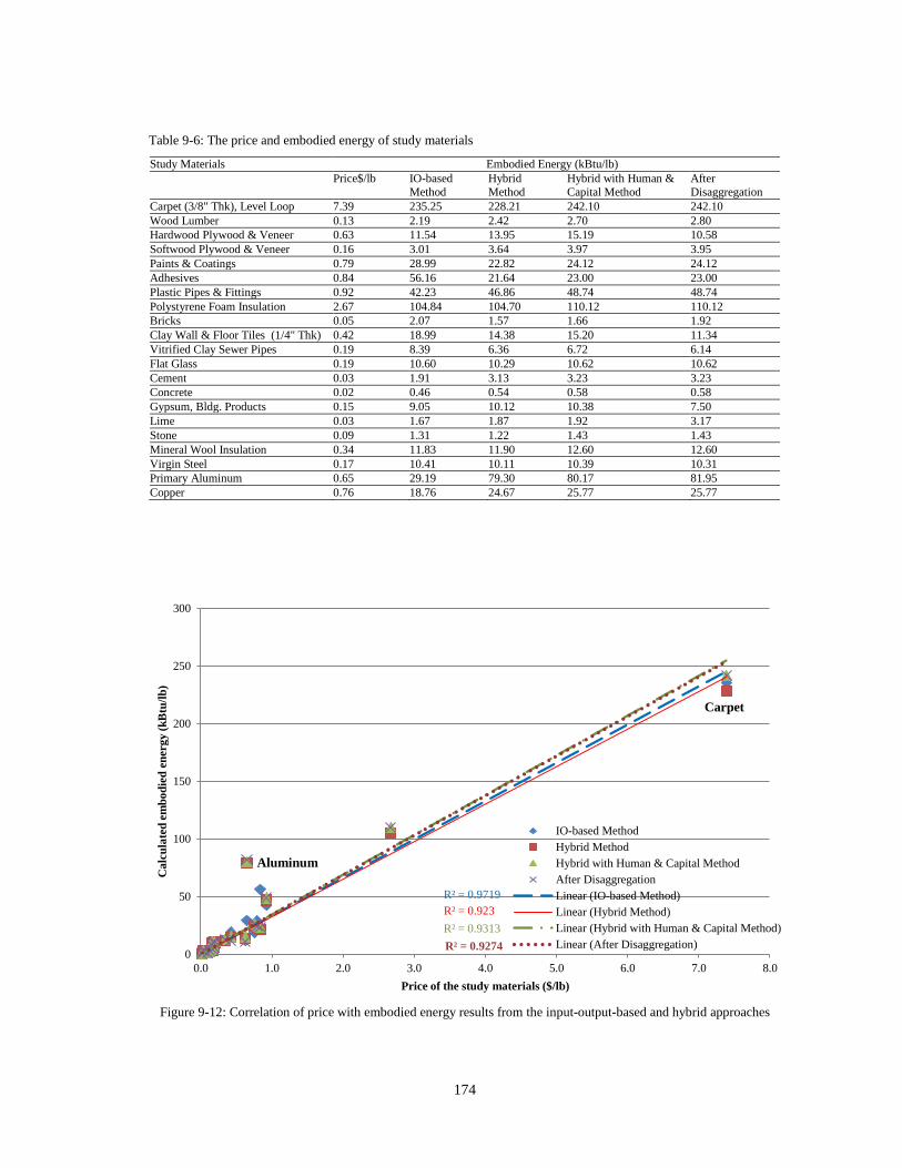
174
Table 9-6: The price and embodied energy of study materials
Study Materials Embodied Energy (kBtu/lb)
Price$/lb IO-based
Method
Hybrid
Method
Hybrid with Human &
Capital Method
After
Disaggregation
Carpet (3/8" Thk), Level Loop 7.39 235.25 228.21 242.10 242.10
Wood Lumber 0.13 2.19 2.42 2.70 2.80
Hardwood Plywood & Veneer 0.63 11.54 13.95 15.19 10.58
Softwood Plywood & Veneer 0.16 3.01 3.64 3.97 3.95
Paints & Coatings 0.79 28.99 22.82 24.12 24.12
Adhesives 0.84 56.16 21.64 23.00 23.00
Plastic Pipes & Fittings 0.92 42.23 46.86 48.74 48.74
Polystyrene Foam Insulation 2.67 104.84 104.70 110.12 110.12
Bricks 0.05 2.07 1.57 1.66 1.92
Clay Wall & Floor Tiles (1/4" Thk) 0.42 18.99 14.38 15.20 11.34
Vitrified Clay Sewer Pipes 0.19 8.39 6.36 6.72 6.14
Flat Glass 0.19 10.60 10.29 10.62 10.62
Cement 0.03 1.91 3.13 3.23 3.23
Concrete 0.02 0.46 0.54 0.58 0.58
Gypsum, Bldg. Products 0.15 9.05 10.12 10.38 7.50
Lime 0.03 1.67 1.87 1.92 3.17
Stone 0.09 1.31 1.22 1.43 1.43
Mineral Wool Insulation 0.34 11.83 11.90 12.60 12.60
Virgin Steel 0.17 10.41 10.11 10.39 10.31
Primary Aluminum 0.65 29.19 79.30 80.17 81.95
Copper 0.76 18.76 24.67 25.77 25.77
Figure 9-12: Correlation of price with embodied energy results from the input-output-based and hybrid approaches
R² = 0.9719
R² = 0.923
R² = 0.9313
R² = 0.9274 0
50
100
150
200
250
300
0.0 1.0 2.0 3.0 4.0 5.0 6.0 7.0 8.0
Ca
lcu
late
d e
mb
od
ied
en
erg
y (
kB
tu/l
b)
Price of the study materials ($/lb)
IO-based Method
Hybrid Method
Hybrid with Human & Capital Method
After Disaggregation
Linear (IO-based Method)
Linear (Hybrid Method)
Linear (Hybrid with Human & Capital Method)
Linear (After Disaggregation)
Aluminum
Carpet

175
Table 9-7: Regression analysis results for price and input-output-based results
SUMMARY OUTPUT Price & Input-output-based Embodied Energy
Regression Statistics
Multiple R 0.989212
R Square 0.978541
Adjusted R Square 0.928541
Standard Error 8.931565
Observations 21
ANOVA
df SS MS F Significance F
Regression 1 72754.63 72754.63 912.0224 1.6E-17
Residual 20 1595.457 79.77286
Total 21 74350.09
Coefficients Standard Error t Stat P-value Lower 95% Upper 95%
Intercept 0 #N/A #N/A #N/A #N/A #N/A
X Variable 1 33.25343 1.101118 30.19971 3.68E-18 30.95654 35.55032
Table 9-8: Regression analysis results for price and input-output-based hybrid analysis results
SUMMARY OUTPUT Price & Input-output-based Hybrid Embodied Energy
Regression Statistics
Multiple R 0.970574
R Square 0.942013
Adjusted R Square 0.892013
Standard Error 14.65269
Observations 21
ANOVA
df SS MS F Significance F
Regression 1 69757.66 69757.66 324.9057 2.09E-13
Residual 20 4294.026 214.7013
Total 21 74051.69
Coefficients Standard Error t Stat P-value Lower 95% Upper 95% Lower 95.0%
Intercept 0 #N/A #N/A #N/A #N/A #N/A #N/A
X Variable 1 32.56132 1.80644 18.02514 7.78E-14 28.79316 36.32949 28.79316
Because the price data were obtained from a range of sources, a correlation analysis was also done for
material prices selected from the 2002 National Construction Estimator, 50th
Edition (Ogershok, 2002).
This was done to ensure that correlation is tested for material prices that were published by the
construction cost guides. Since the study utilized the input-output data from the year 2002, the 2002
version of the cost guide was used. For a few materials, the prices could not be calculated in per unit of
mass, and therefore, prices from Table 9-6 were used. Table A1-12 in Appendix A1 lists the prices
obtained from the National Construction Estimator. Figure 9-13 shows a strong and positive correlation of
material prices and embodied energy calculated using the four approaches. The correlation weakened
slightly due to several reasons. The material prices given in the cost guide included waste factors and also
the cost of additional materials such as glue, nails etc. Hence a different correlation could be expected. The
results of the simple regression analysis are shown in Table 9-9 for the input-output-based hybrid method.
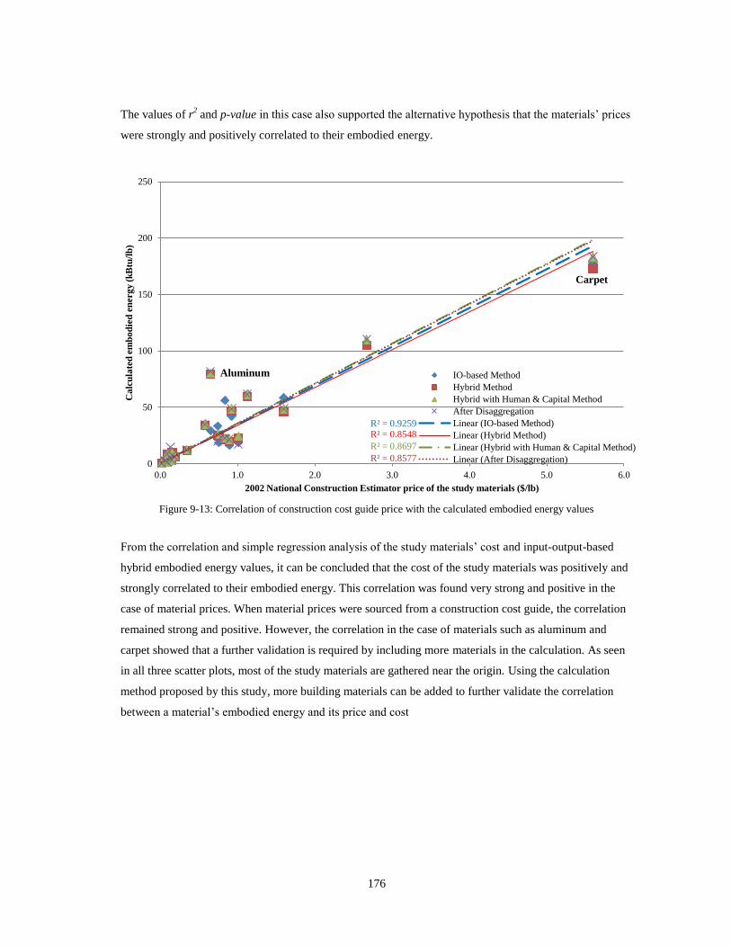
176
The values of r2 and p-value in this case also supported the alternative hypothesis that the materials’ prices
were strongly and positively correlated to their embodied energy.
Figure 9-13: Correlation of construction cost guide price with the calculated embodied energy values
From the correlation and simple regression analysis of the study materials’ cost and input-output-based
hybrid embodied energy values, it can be concluded that the cost of the study materials was positively and
strongly correlated to their embodied energy. This correlation was found very strong and positive in the
case of material prices. When material prices were sourced from a construction cost guide, the correlation
remained strong and positive. However, the correlation in the case of materials such as aluminum and
carpet showed that a further validation is required by including more materials in the calculation. As seen
in all three scatter plots, most of the study materials are gathered near the origin. Using the calculation
method proposed by this study, more building materials can be added to further validate the correlation
between a material’s embodied energy and its price and cost
R² = 0.9259 R² = 0.8548
R² = 0.8697
R² = 0.8577 0
50
100
150
200
250
0.0 1.0 2.0 3.0 4.0 5.0 6.0
Ca
lcu
late
d e
mb
od
ied
en
erg
y (
kB
tu/l
b)
2002 National Construction Estimator price of the study materials ($/lb)
IO-based Method
Hybrid Method
Hybrid with Human & Capital Method
After Disaggregation
Linear (IO-based Method)
Linear (Hybrid Method)
Linear (Hybrid with Human & Capital Method)
Linear (After Disaggregation)
Carpet
Aluminum

177
Table 9-9: Regression analysis results for the construction cost guide prices and input-output-based hybrid results
SUMMARY OUTPUT 2002 National Construction Estimator Price & Input-output-based Hybrid Embodied Energy
Regression Statistics
Multiple R 0.955835
R Square 0.913621
Adjusted R Square
0.863621
Standard Error 15.9976
Observations 21
ANOVA
df SS MS F Significance F
Regression 1 54137.36 54137.36 211.5374 9.46E-12
Residual 20 5118.467 255.9233
Total 21 59255.82
Coefficients Standard
Error
t Stat P-value Lower 95% Upper 95% Lower
95.0%
Upper
95.0%
Intercept 0 #N/A #N/A #N/A #N/A #N/A #N/A #N/A
X Variable 1 33.64688 2.313402 14.54433 4.24E-12 28.82121 38.47255 28.82121 38.47255
9.4 EVALUATION OF RESULTS
9.4.1 Gap Analysis
The gap analysis was performed in order to evaluate the differences the calculated values have with other
methods. As mentioned in the literature review, studies irrespective of what methods they adopted defined
their system boundaries subjectively. This made their results incomparable across studies with different
system boundaries. If the gap is analyzed for process-based embodied energy values with differing system
boundaries, the analysis may not be comparable. In this research, we considered it appropriate to analyze
the gap of process-based (direct energy) and input-output-based energy values with the values calculated
using the hybrid analyses. Such analysis is more valuable because it provides a range of embodied energy
value calculated using a relatively incomplete and a more complete method. In addition, we can measure
how much incompleteness the process-based values might have due to a system boundary truncation.
Table 9-10 shows the results of the gap analysis. The first three columns list the gap between the process-
based energy values and the three hybrid approaches (calculated using Equation 3-2). In these columns, it
was evident that the gaps in the embodied energy values of study materials ranged from 10% to 99% of
the hybrid values, which was significant.
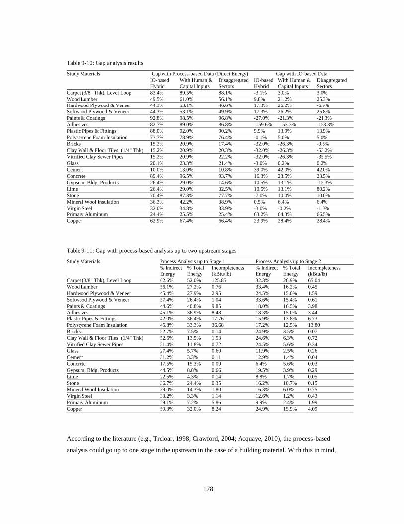
178
Table 9-10: Gap analysis results
Study Materials Gap with Process-based Data (Direct Energy) Gap with IO-based Data
IO-based
Hybrid
With Human &
Capital Inputs
Disaggregated
Sectors
IO-based
Hybrid
With Human &
Capital Inputs
Disaggregated
Sectors
Carpet (3/8" Thk), Level Loop 83.4% 89.5% 88.1% -3.1% 3.0% 3.0%
Wood Lumber 49.5% 61.0% 56.1% 9.8% 21.2% 25.3%
Hardwood Plywood & Veneer 44.3% 53.1% 46.6% 17.3% 26.2% -6.9%
Softwood Plywood & Veneer 44.3% 53.1% 49.9% 17.3% 26.2% 25.8%
Paints & Coatings 92.8% 98.5% 96.8% -27.0% -21.3% -21.3%
Adhesives 82.7% 89.0% 86.8% -159.6% -153.3% -153.3%
Plastic Pipes & Fittings 88.0% 92.0% 90.2% 9.9% 13.9% 13.9%
Polystyrene Foam Insulation 73.7% 78.9% 76.4% -0.1% 5.0% 5.0%
Bricks 15.2% 20.9% 17.4% -32.0% -26.3% -9.5%
Clay Wall & Floor Tiles (1/4" Thk) 15.2% 20.9% 20.3% -32.0% -26.3% -53.2%
Vitrified Clay Sewer Pipes 15.2% 20.9% 22.2% -32.0% -26.3% -35.5%
Glass 20.1% 23.3% 21.4% -3.0% 0.2% 0.2%
Cement 10.0% 13.0% 10.8% 39.0% 42.0% 42.0%
Concrete 89.4% 96.5% 93.7% 16.3% 23.5% 23.5%
Gypsum, Bldg. Products 26.4% 29.0% 14.6% 10.5% 13.1% -15.3%
Lime 26.4% 29.0% 32.5% 10.5% 13.1% 80.2%
Stone 70.4% 87.3% 77.7% -7.0% 10.0% 10.0%
Mineral Wool Insulation 36.3% 42.2% 38.9% 0.5% 6.4% 6.4%
Virgin Steel 32.0% 34.8% 33.9% -3.0% -0.2% -1.0%
Primary Aluminum 24.4% 25.5% 25.4% 63.2% 64.3% 66.5%
Copper 62.9% 67.4% 66.4% 23.9% 28.4% 28.4%
Table 9-11: Gap with process-based analysis up to two upstream stages
Study Materials Process Analysis up to Stage 1 Process Analysis up to Stage 2
% Indirect Energy
% Total Energy
Incompleteness (kBtu/lb)
% Indirect Energy
% Total Energy
Incompleteness (kBtu/lb)
Carpet (3/8" Thk), Level Loop 62.6% 52.0% 125.85 32.3% 26.9% 65.04
Wood Lumber 56.1% 27.2% 0.76 33.4% 16.2% 0.45
Hardwood Plywood & Veneer 45.4% 27.9% 2.95 24.5% 15.0% 1.59
Softwood Plywood & Veneer 57.4% 26.4% 1.04 33.6% 15.4% 0.61
Paints & Coatings 44.6% 40.8% 9.85 18.0% 16.5% 3.98
Adhesives 45.1% 36.9% 8.48 18.3% 15.0% 3.44
Plastic Pipes & Fittings 42.0% 36.4% 17.76 15.9% 13.8% 6.73
Polystyrene Foam Insulation 45.8% 33.3% 36.68 17.2% 12.5% 13.80
Bricks 52.7% 7.5% 0.14 24.9% 3.5% 0.07
Clay Wall & Floor Tiles (1/4" Thk) 52.6% 13.5% 1.53 24.6% 6.3% 0.72
Vitrified Clay Sewer Pipes 51.4% 11.8% 0.72 24.5% 5.6% 0.34
Glass 27.4% 5.7% 0.60 11.9% 2.5% 0.26
Cement 31.2% 3.3% 0.11 12.9% 1.4% 0.04
Concrete 17.5% 15.3% 0.09 6.4% 5.6% 0.03
Gypsum, Bldg. Products 44.5% 8.8% 0.66 19.5% 3.9% 0.29
Lime 22.5% 4.3% 0.14 8.8% 1.7% 0.05
Stone 36.7% 24.4% 0.35 16.2% 10.7% 0.15
Mineral Wool Insulation 39.0% 14.3% 1.80 16.3% 6.0% 0.75
Virgin Steel 33.2% 3.3% 1.14 12.6% 1.2% 0.43
Primary Aluminum 29.1% 7.2% 5.86 9.9% 2.4% 1.99
Copper 50.3% 32.0% 8.24 24.9% 15.9% 4.09
According to the literature (e.g., Treloar, 1998; Crawford, 2004; Acquaye, 2010), the process-based
analysis could go up to one stage in the upstream in the case of a building material. With this in mind,
179
consider a case of the lowest gap (11%), which was for the hybrid values of cement production. If a
process-based analysis is performed covering the indirect inputs up to stage 1, then according to the results
of this study, nearly 69% of the indirect inputs would be accounted for. This leaves a gap or
incompleteness of 31% in the total indirect impacts. If the highest gap (99% for paints and coating) is
considered, this incompleteness could reach up to 45% of the total indirect impacts. Table 9-11 provides
the incompleteness as a percentage of the study materials’ indirect energy and the total embodied energy if
a process-based analysis is carried out up to stage 1 and 2 in the upstream. According to Lenzen (2000)
and Mattila et al. (2010), the process-based analyses could have up to 50% incompleteness in the
embodied energy calculation due to system boundary truncation. The results of this study support their
assertion.
Based on the results of this study, it can be asserted that a process-based analysis, even if performed up to
stage 2, could have significant incompleteness. It is important to note that the values of incompleteness in
embodied energy given in Table 9-11 are per mass of the study material. Looking at the quantities of these
materials routinely used in the construction industry, the incompleteness could be large enough to cause
serious errors in the calculation of the total embodied energy of a building.
The last three columns of Table 9-10 present the gap in the results of the three hybrid approaches and the
input-output-based analysis (calculated using Equation 3-3). The gap ranged from -160% to 80% of the
compared hybrid values. The input-output-based embodied energy values of chemical industries producing
products such as paints and adhesives were quite higher than the hybrid values. One reason for this could
be the variation of energy prices paid by the industry sectors. The chemical industries also consumed large
amounts of petroleum products as an energy source and as a feedstock material. Looking at the chances of
double counting highlighted by the literature (Treloar, 1998; Crawford, 2004), high energy intensity could
be expected. The manufacturing sectors also purchased fuel to generate electricity on-site, which could be
counted twice if the produced electricity and fuel use both were counted in the indirect energy calculation.
In the case of most study materials, the hybrid analysis-based values were higher than the input-output-
based results. This was expected due to two reasons. First, the calculated PEFs for various energy sources
accounted for the direct energy of human and capital inputs and most of the indirect energy inputs. In
addition, the indirect impacts of the imported energy source were included. Therefore, the calculated
values of PEFs were comprehensive. Using these PEFs to convert delivered energy into primary energy
could raise the total energy values. Second, the human and capital energy was counted for each industry
sector that may also have contributed to the total energy intensity.
As a part of the gap analysis, the trend in calculated embodied energy values was examined for
determining the range of embodied energy. Figure 9-14 shows the pattern of embodied energy values
calculated using the three hybrid approaches for some of the study materials. It can be seen that some
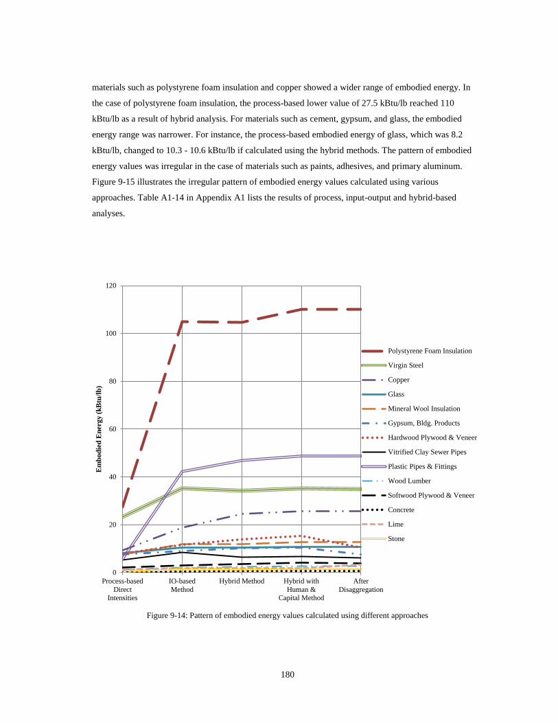
180
materials such as polystyrene foam insulation and copper showed a wider range of embodied energy. In
the case of polystyrene foam insulation, the process-based lower value of 27.5 kBtu/lb reached 110
kBtu/lb as a result of hybrid analysis. For materials such as cement, gypsum, and glass, the embodied
energy range was narrower. For instance, the process-based embodied energy of glass, which was 8.2
kBtu/lb, changed to 10.3 - 10.6 kBtu/lb if calculated using the hybrid methods. The pattern of embodied
energy values was irregular in the case of materials such as paints, adhesives, and primary aluminum.
Figure 9-15 illustrates the irregular pattern of embodied energy values calculated using various
approaches. Table A1-14 in Appendix A1 lists the results of process, input-output and hybrid-based
analyses.
Figure 9-14: Pattern of embodied energy values calculated using different approaches
0
20
40
60
80
100
120
Process-based
DirectIntensities
IO-based
Method
Hybrid Method Hybrid with
Human &Capital Method
After
Disaggregation
Em
bo
die
d E
nerg
y (
kB
tu/l
b)
Polystyrene Foam Insulation
Virgin Steel
Copper
Glass
Mineral Wool Insulation
Gypsum, Bldg. Products
Hardwood Plywood & Veneer
Vitrified Clay Sewer Pipes
Plastic Pipes & Fittings
Wood Lumber
Softwood Plywood & Veneer
Concrete
Lime
Stone
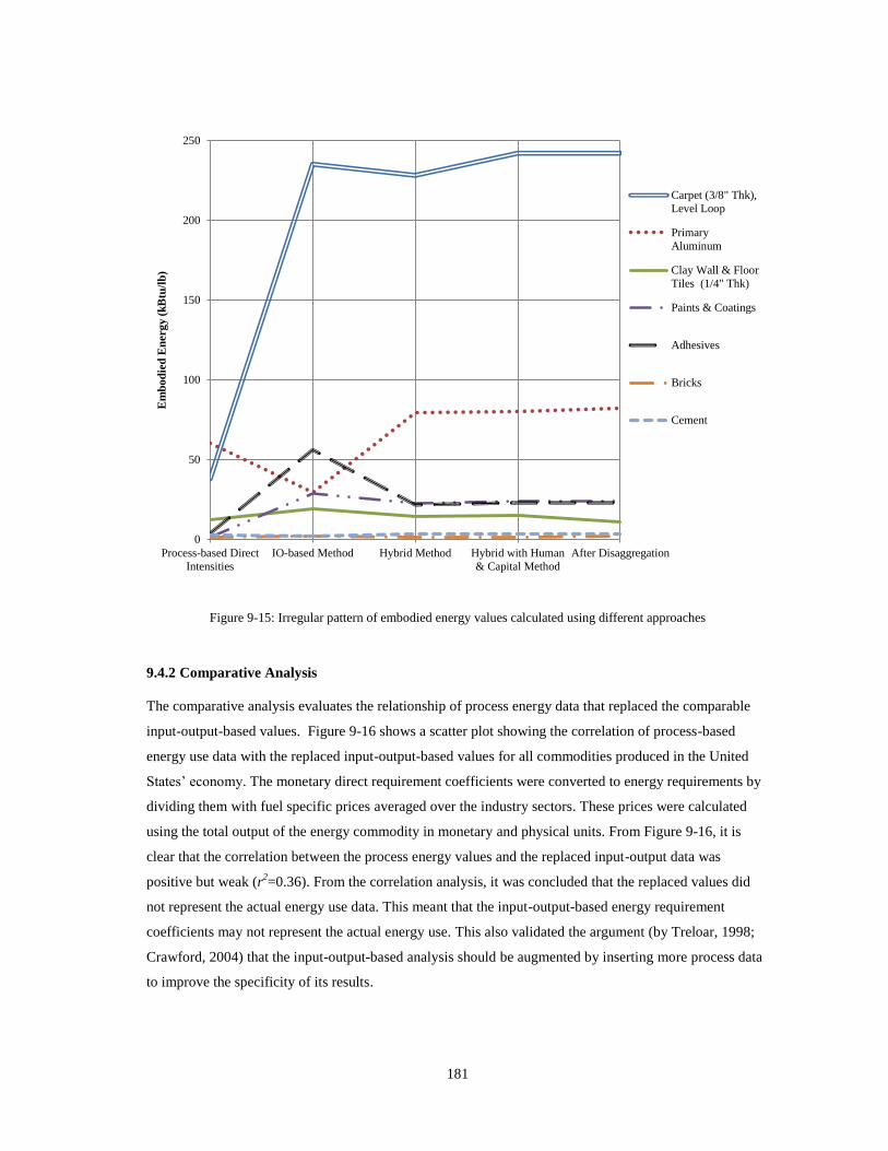
181
Figure 9-15: Irregular pattern of embodied energy values calculated using different approaches
9.4.2 Comparative Analysis
The comparative analysis evaluates the relationship of process energy data that replaced the comparable
input-output-based values. Figure 9-16 shows a scatter plot showing the correlation of process-based
energy use data with the replaced input-output-based values for all commodities produced in the United
States’ economy. The monetary direct requirement coefficients were converted to energy requirements by
dividing them with fuel specific prices averaged over the industry sectors. These prices were calculated
using the total output of the energy commodity in monetary and physical units. From Figure 9-16, it is
clear that the correlation between the process energy values and the replaced input-output data was
positive but weak (r2=0.36). From the correlation analysis, it was concluded that the replaced values did
not represent the actual energy use data. This meant that the input-output-based energy requirement
coefficients may not represent the actual energy use. This also validated the argument (by Treloar, 1998;
Crawford, 2004) that the input-output-based analysis should be augmented by inserting more process data
to improve the specificity of its results.
0
50
100
150
200
250
Process-based Direct
Intensities
IO-based Method Hybrid Method Hybrid with Human
& Capital Method
After Disaggregation
Em
bo
die
d E
nerg
y (
kB
tu/l
b)
Carpet (3/8" Thk),
Level Loop
Primary
Aluminum
Clay Wall & Floor
Tiles (1/4" Thk)
Paints & Coatings
Adhesives
Bricks
Cement
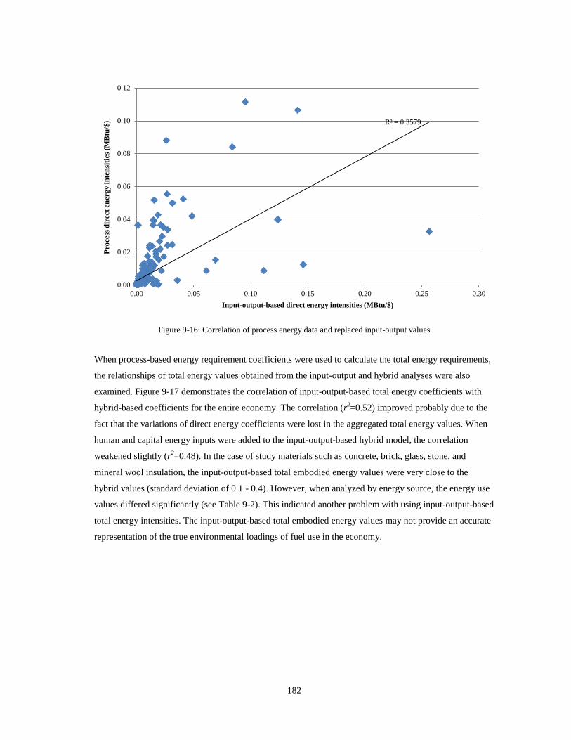
182
Figure 9-16: Correlation of process energy data and replaced input-output values
When process-based energy requirement coefficients were used to calculate the total energy requirements,
the relationships of total energy values obtained from the input-output and hybrid analyses were also
examined. Figure 9-17 demonstrates the correlation of input-output-based total energy coefficients with
hybrid-based coefficients for the entire economy. The correlation (r2=0.52) improved probably due to the
fact that the variations of direct energy coefficients were lost in the aggregated total energy values. When
human and capital energy inputs were added to the input-output-based hybrid model, the correlation
weakened slightly (r2=0.48). In the case of study materials such as concrete, brick, glass, stone, and
mineral wool insulation, the input-output-based total embodied energy values were very close to the
hybrid values (standard deviation of 0.1 - 0.4). However, when analyzed by energy source, the energy use
values differed significantly (see Table 9-2). This indicated another problem with using input-output-based
total energy intensities. The input-output-based total embodied energy values may not provide an accurate
representation of the true environmental loadings of fuel use in the economy.
R² = 0.3579
0.00
0.02
0.04
0.06
0.08
0.10
0.12
0.00 0.05 0.10 0.15 0.20 0.25 0.30
Pro
cess
dir
ect
en
erg
y in
ten
siti
es
(MB
tu/$
)
Input-output-based direct energy intensities (MBtu/$)
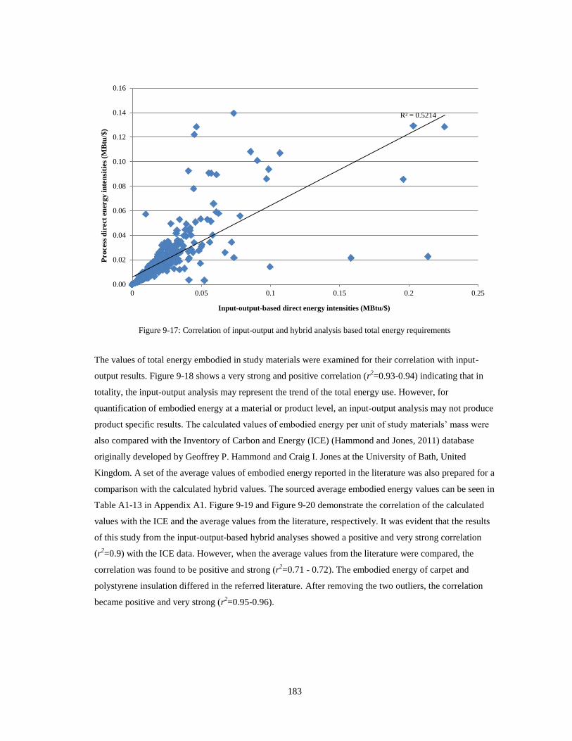
183
Figure 9-17: Correlation of input-output and hybrid analysis based total energy requirements
The values of total energy embodied in study materials were examined for their correlation with input-
output results. Figure 9-18 shows a very strong and positive correlation (r2=0.93-0.94) indicating that in
totality, the input-output analysis may represent the trend of the total energy use. However, for
quantification of embodied energy at a material or product level, an input-output analysis may not produce
product specific results. The calculated values of embodied energy per unit of study materials’ mass were
also compared with the Inventory of Carbon and Energy (ICE) (Hammond and Jones, 2011) database
originally developed by Geoffrey P. Hammond and Craig I. Jones at the University of Bath, United
Kingdom. A set of the average values of embodied energy reported in the literature was also prepared for a
comparison with the calculated hybrid values. The sourced average embodied energy values can be seen in
Table A1-13 in Appendix A1. Figure 9-19 and Figure 9-20 demonstrate the correlation of the calculated
values with the ICE and the average values from the literature, respectively. It was evident that the results
of this study from the input-output-based hybrid analyses showed a positive and very strong correlation
(r2=0.9) with the ICE data. However, when the average values from the literature were compared, the
correlation was found to be positive and strong (r2=0.71 - 0.72). The embodied energy of carpet and
polystyrene insulation differed in the referred literature. After removing the two outliers, the correlation
became positive and very strong (r2=0.95-0.96).
R² = 0.5214
0.00
0.02
0.04
0.06
0.08
0.10
0.12
0.14
0.16
0 0.05 0.1 0.15 0.2 0.25
Pro
cess
dir
ect
en
erg
y in
ten
siti
es
(MB
tu/$
)
Input-output-based direct energy intensities (MBtu/$)
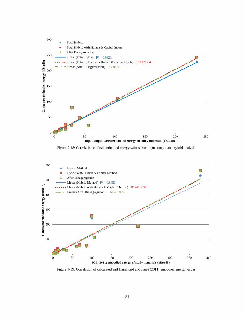
184
Figure 9-18: Correlation of final embodied energy values from input-output and hybrid analysis
Figure 9-19: Correlation of calculated and Hammond and Jones (2011) embodied energy values
R² = 0.9323
R² = 0.9384
R² = 0.935
0
50
100
150
200
250
300
0 50 100 150 200 250
Ca
lcu
late
d e
mb
od
ied
en
erg
y (
kB
tu/l
b)
Input-output-based embodied energy of study materials (kBtu/lb)
Total Hybrid
Total Hybrid with Human & Capital Inputs
After Disaggregation
Linear (Total Hybrid)
Linear (Total Hybrid with Human & Capital Inputs)
Linear (After Disaggregation)
R² = 0.8952
R² = 0.8897
R² = 0.8958
0
100
200
300
400
500
600
0 50 100 150 200 250 300 350 400
Ca
lcu
late
d e
mb
od
ied
en
erg
y (
kB
tu/l
b)
ICE (2011) embodied energy of study materials (kBtu/lb)
Hybrid Method
Hybrid with Human & Capital Method
After Disaggregation
Linear (Hybrid Method)
Linear (Hybrid with Human & Capital Method)
Linear (After Disaggregation)
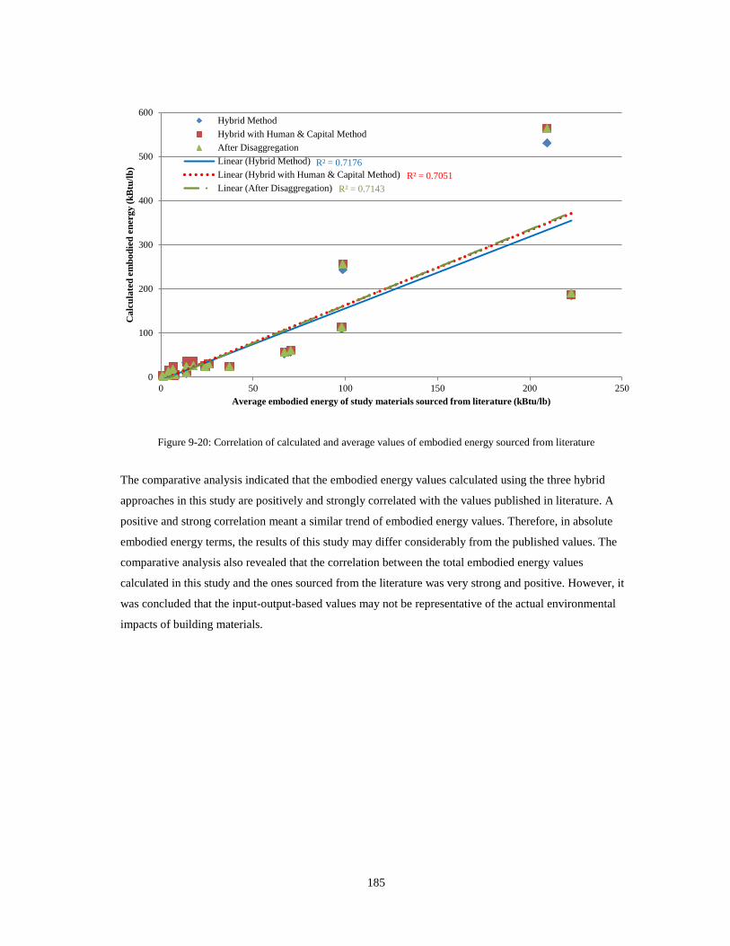
185
Figure 9-20: Correlation of calculated and average values of embodied energy sourced from literature
The comparative analysis indicated that the embodied energy values calculated using the three hybrid
approaches in this study are positively and strongly correlated with the values published in literature. A
positive and strong correlation meant a similar trend of embodied energy values. Therefore, in absolute
embodied energy terms, the results of this study may differ considerably from the published values. The
comparative analysis also revealed that the correlation between the total embodied energy values
calculated in this study and the ones sourced from the literature was very strong and positive. However, it
was concluded that the input-output-based values may not be representative of the actual environmental
impacts of building materials.
R² = 0.7176
R² = 0.7051
R² = 0.7143
0
100
200
300
400
500
600
0 50 100 150 200 250
Ca
lcu
late
d e
mb
od
ied
en
erg
y (
kB
tu/l
b)
Average embodied energy of study materials sourced from literature (kBtu/lb)
Hybrid Method
Hybrid with Human & Capital Method
After Disaggregation
Linear (Hybrid Method)
Linear (Hybrid with Human & Capital Method)
Linear (After Disaggregation)
186
CHAPTER X
DISCUSSION
10.
10.1 GUIDELINES FOR EMBODIED ENERGY CALCULATION
The review of literature revealed a need for a set of guidelines for streamlining the embodied energy
calculation process. The international standards such as ISO 14040 and ISO 14044 were developed
originally for providing guidance to the process of Life Cycle Assessment (LCA). Some studies mentioned
applying these standards to their research. However, literature (Suh et al., 2004; Weidema et al., 2008;
Zamagni et al., 2008) supported that the ISO standards in their current form provide very little guidance to
an embodied energy analysis or LCA. Some critics also said that some of the requirements mentioned in
the ISO standards are open to interpretation; as a result, subjectivity has become a major issue with LCA.
In this research, the four most important embodied energy parameters were streamlined. First, a definition
of embodied energy was proposed based on the opinion of literature. Other related terms such as life cycle
embodied energy, operating energy, and life cycle energy were also defined. The main purpose of defining
these terms was to clarify and standardize their meaning. The second parameter relates to the system
boundary model. A building is a large and complex product, and its design and construction is unique to
each case. In defining a system to calculate the embodied energy of the building, various aspects need to
be considered. If the energy use of the building is analyzed on the basis of just the initial embodied energy,
the analysis may not be valid. For a comprehensive and genuine energy evaluation, it is important to
perform the energy accounting of the whole life cycle of the building. In this study, various system
boundary models were synthesized to propose one model that is complete.
The third parameter is embodied energy calculation method. Various methods have been proposed
including process-based and input-output-based analyses. Each method has both advantages and
disadvantages. As a result, various combinations of these methods were developed in order to reduce their
disadvantages. However, there is still no consensus on which method to use for calculating the embodied
energy. Looking at the system boundary model emphasized by the literature, an input-output-based hybrid
analysis seems more appropriate. The biggest advantage of an input-output-based hybrid analysis is that it
is complete. Although its results, in some cases, are regarded as less specific to the study, various
approaches to address this issue were also proposed. Economic input-output models across the globe are
becoming more disaggregated, and with the readily available energy data, a more robust input-output-
based model could be developed in the future. Based on the results of this study, it would be fair to say
that the chances of improving the specificity of an input-output-based method are greater than making a

187
process-based analysis complete. To standardize the calculation of embodied energy, an input-output-
based hybrid approach was proposed in this study.
The last parameter is about using energy and nonenergy data in the calculation. Two aspects of the used
data are important: completeness and representativeness. If these aspects of the data are not clear, they
should not be incorporated in the study. The guidelines for reporting results of the study were also
proposed. One major issue with energy reporting is that the energy results are provided in either delivered
or primary energy form without describing any conversion factors. Such results in different energy units
cannot be compared, and hence, could not be applied.
10.2 EMBODIED ENERGY CALCULATION METHOD
10.2.1 Input-output Model
The latest input-output data published by the United States Bureau of Economic Analysis is available from
2002. The commodity-by-commodity matrix is highly disaggregated, and hence, provides a robust model
in terms of specificity. Although assumptions of proportionality and homogeneity still exist, the process of
redefinition helps reduce some of the impacts of these assumptions. The coefficient of direct requirements
is the most influential parameter for calculating the total requirements. If an industry sector buys more to
produce a unit dollar of its output, its indirect requirements also increase. This assertion assumes that the
direct requirements govern the total requirements. While creating the model, it was observed that there
may be serious issues with this assumption. For instance, there are sectors that do not consume everything
they purchase, as they may be reselling the purchased materials. In monetary terms, this may be
appropriate but for the energy use analysis, it may cause double counting. For sectors such as retail and
wholesale trade, the total purchases from energy providing sectors are quite large. However, most of the
energy may be purchased to be traded. Such aspects are not clear in the direct and total requirements.
10.2.2 Process Data of Direct Energy Use
The energy data provided for most manufacturing industries were in both the monetary and energy units,
whereas for other sectors they were mostly in monetary units. However, some sector specific energy prices
were also available to convert the energy use from monetary to energy units. One major issue with the
energy data is that some of the data are either missing or are highly aggregated. However, input-output-
based monetary flows can be used to disaggregate the total energy use. Some manufacturing sectors
purchased fuel and used a fraction of it in on-site electricity production. According to MECS data, this
electricity is either used by the sector completely, sold out to other sectors, or transferred to other
industries within the sector. If no monetary transactions occurred, the flow of electricity may not be
recorded in the input-output model. To avoid the double counting and completely account for each energy
input it is important to consider only inputs that are primary energy. For instance, if all fuel purchases of
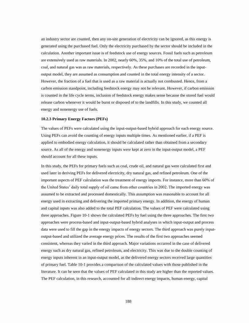
188
an industry sector are counted, then any on-site generation of electricity can be ignored, as this energy is
generated using the purchased fuel. Only the electricity purchased by the sector should be included in the
calculation. Another important issue is of feedstock use of energy sources. Fossil fuels such as petroleum
are extensively used as raw materials. In 2002, nearly 60%, 35%, and 10% of the total use of petroleum,
coal, and natural gas was as raw materials, respectively. As these purchases are recorded in the input-
output model, they are assumed as consumption and counted in the total energy intensity of a sector.
However, the fraction of a fuel that is used as a raw material is actually not combusted. Hence, from a
carbon emission standpoint, including feedstock energy may not be relevant. However, if carbon emission
is counted in the life cycle terms, inclusion of feedstock energy makes sense because the stored fuel would
release carbon whenever it would be burnt or disposed of to the landfills. In this study, we counted all
energy and nonenergy use of fuels.
10.2.3 Primary Energy Factors (PEFs)
The values of PEFs were calculated using the input-output-based hybrid approach for each energy source.
Using PEFs can avoid the counting of energy inputs multiple times. As mentioned earlier, if a PEF is
applied to embodied energy calculation, it should be calculated rather than obtained from a secondary
source. As all of the energy and nonenergy inputs were kept at zero in the input-output model, a PEF
should account for all these inputs.
In this study, the PEFs for primary fuels such as coal, crude oil, and natural gas were calculated first and
used later in deriving PEFs for delivered electricity, dry natural gas, and refined petroleum. One of the
important aspects of PEF calculation was the treatment of energy imports. For instance, more than 60% of
the United States’ daily total supply of oil came from other countries in 2002. The imported energy was
assumed to be extracted and processed domestically. This assumption was reasonable to account for all
energy used in extracting and delivering the imported primary energy. In addition, the energy of human
and capital inputs was also added to the total PEF calculation. The values of PEF were calculated using
three approaches. Figure 10-1 shows the calculated PEFs by fuel using the three approaches. The first two
approaches were process-based and input-output-based hybrid analyses in which input-output and process
data were used to fill the gap in the energy impacts of energy sectors. The third approach was purely input-
output-based and utilized the average energy prices. The results of the first two approaches seemed
consistent, whereas they varied in the third approach. Major variations occurred in the case of delivered
energy such as dry natural gas, refined petroleum, and electricity. This was due to the double counting of
energy inputs inherent in an input-output model, as the delivered energy sectors received large quantities
of primary fuel. Table 10-1 provides a comparison of the calculated values with those published in the
literature. It can be seen that the values of PEF calculated in this study are higher than the reported values.
The PEF calculation, in this research, accounted for all indirect energy impacts, human energy, capital
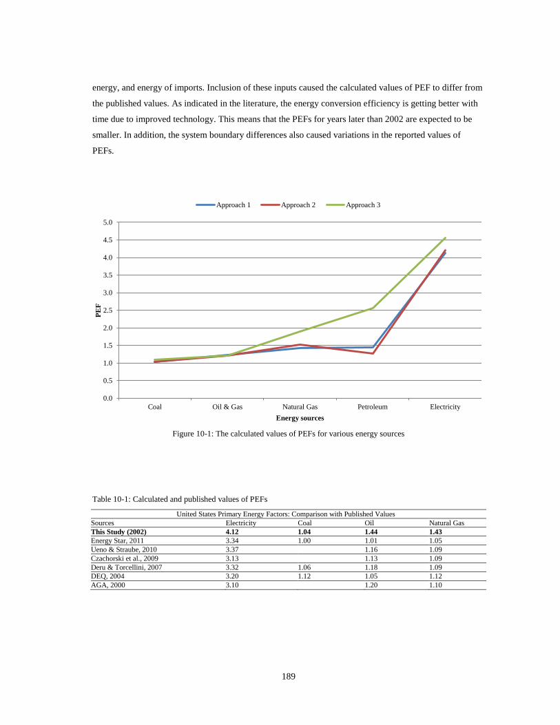
189
energy, and energy of imports. Inclusion of these inputs caused the calculated values of PEF to differ from
the published values. As indicated in the literature, the energy conversion efficiency is getting better with
time due to improved technology. This means that the PEFs for years later than 2002 are expected to be
smaller. In addition, the system boundary differences also caused variations in the reported values of
PEFs.
Figure 10-1: The calculated values of PEFs for various energy sources
Table 10-1: Calculated and published values of PEFs
United States Primary Energy Factors: Comparison with Published Values
Sources Electricity Coal Oil Natural Gas
This Study (2002) 4.12 1.04 1.44 1.43
Energy Star, 2011 3.34 1.00 1.01 1.05
Ueno & Straube, 2010 3.37 1.16 1.09
Czachorski et al., 2009 3.13 1.13 1.09
Deru & Torcellini, 2007 3.32 1.06 1.18 1.09
DEQ, 2004 3.20 1.12 1.05 1.12
AGA, 2000 3.10 1.20 1.10
0.0
0.5
1.0
1.5
2.0
2.5
3.0
3.5
4.0
4.5
5.0
Coal Oil & Gas Natural Gas Petroleum Electricity
PE
F
Energy sources
Approach 1 Approach 2 Approach 3

190
10.2.4 Modifications to Input-output Matrix
Although the United States’ economic input-output accounts were highly disaggregated, three
improvements were performed in the model. First, the process energy data were directly inserted in the use
table. This avoided using the national average energy prices. However, in the case of the sectors such as
service industries, energy data were available in monetary units. Instead of using energy prices, we allotted
the total energy use to each sector using the share of each in the total energy purchases using the input-
output data.
Second, human and capital energy inputs were also added to each industry. Although the energy of food
was calculated in detail, the energy embodied in other expenses was estimated deriving a fixed percentage.
For instance, nearly 27 - 30% of other expenses such as clothing and transportation were allotted to the
employment. This area of research still needs a lot of work, as estimation based on a fixed percentage may
not be representative. The capital investment accounts are not published in a timely manner. The energy
embodied in capital goods can be calculated by gathering the data about the capital investments in
buildings, automobiles, equipment, and software using a variety of sources. A detailed account of capital
expenses was only available for a few sectors such as manufacturing. The argument given in the literature
(e.g., Gao et al., 2001; Alcorn, 1997 cited by Crawford, 2004) that the energy embodied in human and
capital goods may not be significant was not supported by the results of this study. In some sectors,
producing items such as dimension stone, the embodied energy of human and capital inputs accounted for
nearly 15% of the total embodied energy. This is significant especially in the case of countries such as
India and China where the industry sectors are still more labor intensive. In this study, the lowest fraction
of human and capital energy was 1.1% for primary aluminum, which was probably due to a much higher
use of other energy sources.
Third, some of the industry sectors that produced more than one item were disaggregated to produce
material-specific embodied energy results. Joshi (1998) discussed various models that can be introduced to
modify the input-output tables for obtaining the desired results. The detailed input and output information
was available from the USCB. However, this information was of little help, as most inputs were clumped
together under the category of “not specified by kind” or “nsk.” The change in total embodied energy due
to disaggregation was within a range of 0.4% to 66%. Table 10-2 lists values of various embodied energy
components before and after disaggregation. It can be seen that in some cases, the disaggregation may
result in significant changes to the total energy intensities.
It was observable that the energy intensity was reduced only when the other products manufactured by the
industry sectors were more energy intensive than the material under study. For instance, the intensity of
virgin steel production reduced slightly due to a higher energy intensity of ferro-alloy products. The
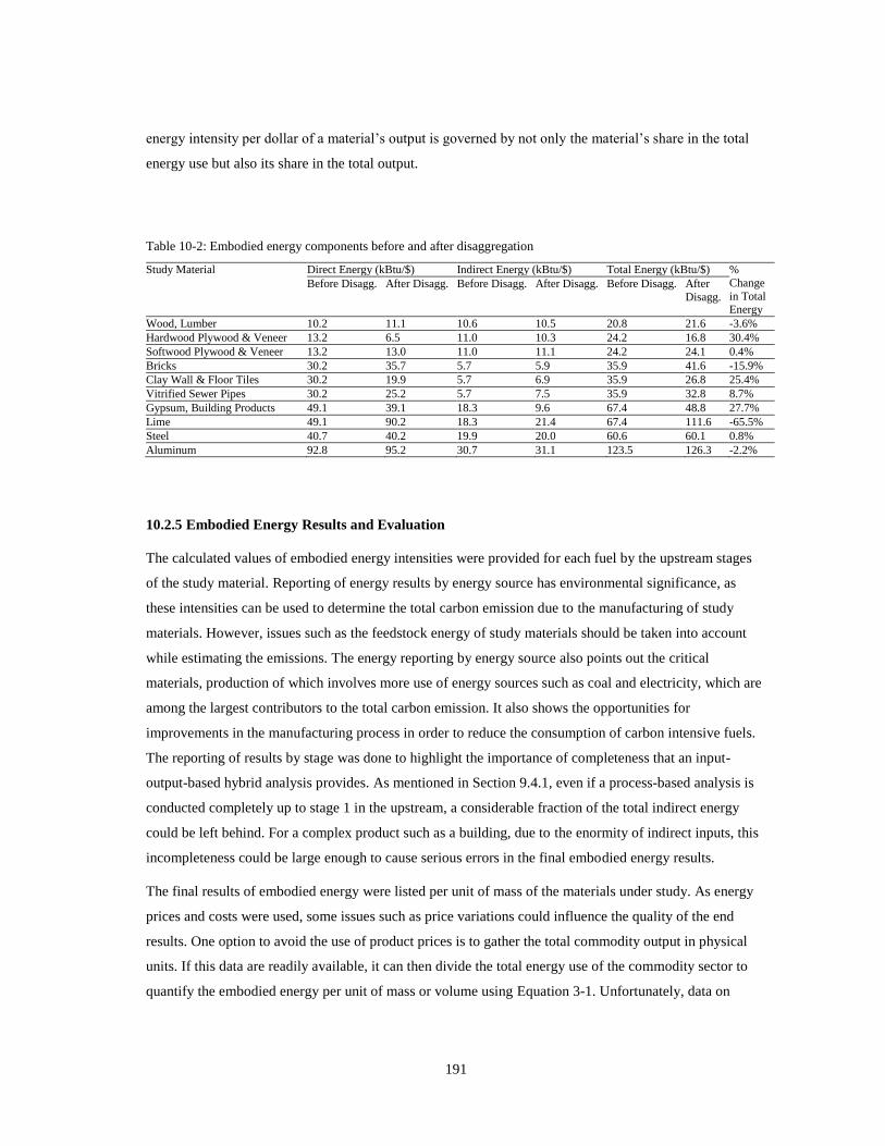
191
energy intensity per dollar of a material’s output is governed by not only the material’s share in the total
energy use but also its share in the total output.
Table 10-2: Embodied energy components before and after disaggregation
Study Material Direct Energy (kBtu/$) Indirect Energy (kBtu/$) Total Energy (kBtu/$) %
Change
in Total Energy
Before Disagg. After Disagg. Before Disagg. After Disagg. Before Disagg. After
Disagg.
Wood, Lumber 10.2 11.1 10.6 10.5 20.8 21.6 -3.6%
Hardwood Plywood & Veneer 13.2 6.5 11.0 10.3 24.2 16.8 30.4%
Softwood Plywood & Veneer 13.2 13.0 11.0 11.1 24.2 24.1 0.4%
Bricks 30.2 35.7 5.7 5.9 35.9 41.6 -15.9%
Clay Wall & Floor Tiles 30.2 19.9 5.7 6.9 35.9 26.8 25.4%
Vitrified Sewer Pipes 30.2 25.2 5.7 7.5 35.9 32.8 8.7%
Gypsum, Building Products 49.1 39.1 18.3 9.6 67.4 48.8 27.7%
Lime 49.1 90.2 18.3 21.4 67.4 111.6 -65.5%
Steel 40.7 40.2 19.9 20.0 60.6 60.1 0.8%
Aluminum 92.8 95.2 30.7 31.1 123.5 126.3 -2.2%
10.2.5 Embodied Energy Results and Evaluation
The calculated values of embodied energy intensities were provided for each fuel by the upstream stages
of the study material. Reporting of energy results by energy source has environmental significance, as
these intensities can be used to determine the total carbon emission due to the manufacturing of study
materials. However, issues such as the feedstock energy of study materials should be taken into account
while estimating the emissions. The energy reporting by energy source also points out the critical
materials, production of which involves more use of energy sources such as coal and electricity, which are
among the largest contributors to the total carbon emission. It also shows the opportunities for
improvements in the manufacturing process in order to reduce the consumption of carbon intensive fuels.
The reporting of results by stage was done to highlight the importance of completeness that an input-
output-based hybrid analysis provides. As mentioned in Section 9.4.1, even if a process-based analysis is
conducted completely up to stage 1 in the upstream, a considerable fraction of the total indirect energy
could be left behind. For a complex product such as a building, due to the enormity of indirect inputs, this
incompleteness could be large enough to cause serious errors in the final embodied energy results.
The final results of embodied energy were listed per unit of mass of the materials under study. As energy
prices and costs were used, some issues such as price variations could influence the quality of the end
results. One option to avoid the use of product prices is to gather the total commodity output in physical
units. If this data are readily available, it can then divide the total energy use of the commodity sector to
quantify the embodied energy per unit of mass or volume using Equation 3-1. Unfortunately, data on

192
actual quantities of production in physical units are not readily available for most of the materials.
Availability of detailed monthly product prices can also help reduce the uncertainties associated with using
the product prices for energy calculation.
The calculated values were found to be in accordance with the published values. Their strong and positive
correlation demonstrated a similar pattern of energy intensities to the published results. Some values
varied most probably due to the product price variations. For instance, the embodied energy of aluminum,
when calculated using the aluminum price, was roughly 80.0 kBtu/lb. When the aluminum cost (calculated
using Equation 3-1) was used, the total embodied energy was approximately 175 kBtu/lb. These results
pointed out a serious problem with converting energy intensities per unit of dollar to per unit of mass.
Solving this problem does not require more research at the embodied energy calculation level but a
detailed and accurate reporting of production data in physical units. The energy intensities resulted from
the hybrid approaches were complete and consistent in their results. The problem arises when these are
converted to embodied energy per unit of mass. Another issue with using product prices relates to the
aggregated sectorial output. For instance, in the case of steel manufacturing, both the raw steel and other
structural shapes (rebar, I-section, round pipe, etc.) were manufactured. If the price of steel is used, it may
underestimate the embodied energy of structural shapes. There may be an overestimation of embodied
energy of raw steel if the price of structural shapes is used. A weighted average price can be calculated on
the basis of proportion of each in the total output and used in the calculation but it may not be
representative of their actual prices.
The input-output data on energy use did not represent the actual energy use as indicated by the
comparative analysis. There could be several reasons for this as stated earlier in Section 9.2.1. The double
counting of energy inputs and the complexity of energy transfer within the sectors are among them. If the
total embodied energy calculated by input-output analysis and by input-output-based hybrid analysis are
compared, they were positively and strongly correlated. Their absolute values per unit of mass may not be
close, but the pattern of energy per unit of mass was quite similar. The hypotheses’ tests revealed a
positive and strong correlation between the price (and cost) and the embodied energy of the study
materials. This finding is significant, especially looking at the studies that suggested a strong and positive
correlation between the energy and the cost. However, the correlation of material cost and price with the
embodied energy needs further validation in order to use the material cost and price as predictors of the
embodied energy.
193
CHAPTER XI
CONCLUSIONS
11.
The impact of a growing global population and a rising standard of living are exerting pressure on the
globe’s capacity to maintain a balanced natural capital. With more people migrating from rural to urban
areas in the future, the situation of resource consumption would only get worse. The use of energy, mostly
fossil fuels, for fuel and non-fuel purposes is getting bigger and bigger. The construction industry,
particularly buildings that currently consume an extensive amount of energy can bring a significant change
if the whole life cycle energy use of buildings is optimized. For this purpose, both the operating and
embodied energy use over a building’s life cycle should be reduced. However, the focus of energy
research remained mostly on the optimization of operating energy. There were several reasons for this.
The existing embodied energy data are either not available or available with issues of inconsistency,
incompleteness, and non-representativeness. To add to the problems, no efforts have been made to define
the term “embodied energy.” Very little guidance is available to calculate embodied energy in a standard
manner. There are no guidelines that can streamline the embodied energy calculation by consistently
defining the system boundaries and by using quality data. The available methods for energy calculation
have various advantages and disadvantages. Some remarkable efforts by Stein et al. (1981), Treloar
(1998), and Crawford (2004), helped in developing a method that is complete and can provide more study-
specific results. However, there were still areas of improvement in the proposed methods.
In this research, an input-output-based hybrid approach was developed to calculate the embodied energy
of construction materials. A set of guidelines for standardizing the process of embodied energy analysis
was also proposed. The current form of input-output-based hybrid analysis can be improved by inserting
process energy data. A thorough understanding of input-output accounts and energy flows in the economy
is vital to avoid issues such as double counting of inputs. It was found that the use of PEFs, originally
proposed by Treloar (1998), can avoid the issue of double counting of energy sources. It was also
concluded that the PEFs should be calculated in a complete manner ensuring that all direct and indirect
inputs associated with an energy source extraction, processing, and delivery are included in the factors. In
addition, human and capital energy inputs not only can be quantified but also can be incorporated into the
economic model. Based on the results of this study, it was concluded that the energy embodied in these
inputs could be significant (up to 15% of the total), and hence, should not be ignored. It was also found
that the results of an input-output-based hybrid approach can be made more product-specific in the future.
However, achieving the same degree of completeness in a process-based analysis seems impractical. For
instance, it was demonstrated that if detailed information on sectorial inputs and outputs is available, the

194
process of sector disaggregation can be used to improve the specificity of the embodied energy results.
Currently, the availability of detailed information on inputs and outputs of industry sectors is limited.
However, in the future, this information may be readily available.
Conventionally, prices of products are sourced to convert the energy intensities per dollar to energy use
per mass or volume. As the prices could be underestimated or overestimated, the end results may have
uncertainties. An approach to calculate the energy intensity per unit of mass was also proposed but it
requires reliable data on the total production in physical units, which is only available for some industry
sectors currently. A significant portion of the total fuel use was consumed as a raw material, which should
be noted especially when using the embodied energy to quantify the resulting carbon emissions.
The relationship of embodied energy and cost of a product has been highlighted in the literature. Costanza
(1980) had supported the positive correlation of cost and embodied energy. Recently, Ding (2004) and
recently Langston (2006) found a strong and positive correlation between the capital cost and the total
embodied energy of a building. However, when the analysis was performed at a component or product
level the correlation weakened. In this research, it was hypothesized that there is a strong and positive
correlation between the price (and cost) and embodied energy of a product. The input-output-based hybrid
approach was modified to calculate the energy embodied in 21 commonly used building materials to test
the hypotheses. Based on the results, it was concluded that the price and cost of a product shared a strong
and positive correlation with its total embodied energy. Hence, the cost or a price of a product can be used
for determining the total energy impacts of manufacturing and using a product. This finding is significant
especially when looking at the three dimensions of a sustainable system: economics, environment, and
society. In a life cycle term, monetary savings could mean proportional savings in the energy use.
However, before prediction the embodied energy form the cost and price, a validation of positive
correlation by incorporating more materials should be done. In addition, it should also be checked if the
relationship is linear or nonlinear. A widely used information tool such as the Computer-Aided Design
(CAD) or Building Information Model (BIM) can be used to estimate the total embodied energy of a
construction project, if embodied energy can be predicted from the cost data. This not only can simplify
the whole embodied energy calculation process but also help in its widespread application in the process
of whole building energy accounting.
To summarize, three main improvements were done to the current form of the input-output-based hybrid
analysis. First, the actual energy use data in energy units was inserted into the input-output model. Second,
the energy embodied in human and capital inputs was quantified and added to the input-output model.
Third, the process of sector disaggregation was demonstrated using the 2002 Benchmark Input-output
data. In addition, in this research, the PEF for each energy source was calculated in a complete manner.
Also, A method is proposed to convert the energy intensities per unit of monetary output into the

195
embodied energy per unit of mass without using the volatile material and energy prices. Among the most
significant values of this research was the demonstration that the energy embodied in a product can be
calculated in a complete and standardized manner with results specific to the product under study. One of
the biggest surprises of this study was the positive and strong correlation of a material’s price and its
embodied energy. The fact that the correlation became stronger after adding the human and capital inputs
was also surprising. This fact also suggested that adding more and more missing inputs (e.g. human and
capital inputs) to the input-output-model would make it more robust for the use of embodied energy
analysis.
11.1 FUTURE RESEARCH
A further investigation into the correlation of cost and price with embodied energy is necessary. A
correlation analysis by material types such as metal, minerals, and plastic products may also be useful in
deriving an equation to predict embodied energy from cost and price data. This study can also be extended
to include more construction materials in the research to test the correlation of material prices and costs
with embodied energy. A series of equations then can be derived to develop a tool that can be used to
calculate the energy embodied in a product using its cost or price. At this stage, a rigorous evaluation of
results would be necessary. A case study of a wide range of construction materials can be performed to
investigate whether the results of the tool are reliable.
Such tools can be integrated into a CAD or a BIM platform. Currently, there is no single tool that can
perform the whole building energy accounting. For instance, if an embodied energy tool is used to select a
low embodied energy material, it is still not known what effects this material may have on a building’s
operating energy. For doing that, one needs to use another tool that can simulate the operating energy
performance. In the whole process one may end up switching back and forth between the embodied and
operating energy tools. The whole process becomes not only tedious but also time and resource
consuming. If a single information tool, such as BIM, can be augmented with capabilities to evaluate the
embodied and operating energy performance, it could save a significant amount of time and resources.
Another venue for future research lies in the field of input-output analysis. A more robust approach can be
developed to disaggregate the industry sectors so that more product-specific values of embodied energy
can be calculated in a complete manner. If capital expenditure accounts are available in a timely manner,
they can be inserted into the economic model to account for capital energy in the total embodied energy in
a more reliable manner.
196
REFERENCES
Abanda, F. H., Tah, J. H. M., and Cheung, F. K. T. (2012). “Mathematical modeling of embodied energy,
greenhouse gases, waste, time-cost parameters of building projects: A Review.” Building and
Environment, 59, 23-37.
ACHP (1979). Assessing the energy conservation benefits of historic preservation: Methods and
Examples. Advisory Council on Historic Preservation, Washington D.C., USA.
Acquaye, A. (2010). A stochastic hybrid embodied energy and CO 2_eq intensity analysis of building and
construction processes in Ireland. Ph.D. Thesis, Dublin Institute of Technology, Dublin, 2010.
Adalberth, K. (1997 a). “Energy use during the life cycle of buildings: a method.” Building and
Environment, 32(4), 317-320.
Adalberth, K. (1997 b). “Energy use during the life cycle of single-unit dwellings: examples.” Building
and Environment, 32(4), 321-329.
Alcorn, A. (1996). Embodied energy coefficient of building materials. Centre for Building Performance
and Research, Victoria University of Wellington, Wellington, NZ.
Alcorn, A. (2003). Embodied energy and CO2 coefficients for NZ building materials. Centre for Building
Performance and Research, Victoria University of Wellington, Wellington, NZ.
Alcorn, J.A., and Baird, G. (1996). Use of a hybrid energy analysis method for evaluating the embodied
energy of building materials. Center for building performance and research, Victoria University
of Wellington, NZ.
Alcott, B. (2012). “Population matters in ecological economics.” Ecological Economics, 80, 109-120.
Almeida, M. G. D., Bragança, L., and Mendonça, P. (2005). Potentialities of lightweight construction
solutions for sustainability. Civil Engineering Department, University of Minho, Guimarães,
Portugal
Alshboul, A.A., and Alzoubi, H.H. (2008). “Analysis of embodied energy requirements for natural
dimensioned stone production in Jordan.” Architectural Science Review, 51(2), 124-132.
Ambler, C. A. (1998, August). “NAICS and US statistics.” In Proceedings of the Section on Government
Statistics and the Section on Social Statistics, American Statistical Association (pp. 21-30).
ARB (2009). Detailed California-modified GREET pathway for Liquefied Natural Gas (LNG) from North
American and remote natural gas sources. July 20, 2009, Air Resources Board, California
Environmental Protection Agency, Sacramento, CA, USA.
Ardente, F., Beccali, M., Cellura, M., and Mistretta, M. (2008). “Building energy performance: a LCA
case study of kenaf-fibres insulation board.” Energy and Buildings, 40(1), 1-10.

197
Asif, M., Muneer, T., and Kelley, R. (2007). “Life cycle assessment: a case study of a dwelling home in
Scotland.” Building and Environment, 42(3), 1391-1394.
ASMI (2009). A life cycle assessment study of embodied effects for existing historic buildings. Athena
Sustainable Materials Institute, Ontario, Canada.
Aste, N., Adhikari, R. S., and Buzzetti, M. (2010). “Beyond the EPBD: the low energy residential
settlement Borgo Solare.” Applied Energy, 87(2), 629-642.
Atkinson, C. (1996). “Life cycle embodied energy and carbon dioxide emissions in buildings.” Industry
and Environment, 19(2), 29-31.
Baird, G., Treleaven, C., and Storey, J. (1994). “The embodiment of embodied energy–a New Zealand
perspective.” In Sustainable construction: Proceedings of the First International Conference of
CIB TG 16, November 6-9, 1994, Tampa, Florida, USA (p. 251).
Baouendi, R., Zmeureanu, R., and Bradley, B. (2005). “Energy and emission estimator: A prototype tool
for designing Canadian houses.” Journal of architectural engineering, 11(2), 50-59.
Barnes, D., and Rankin, L. (1975). “The energy economics of building construction”, Building
International, 8, 31-42.
BESR (2007). Coal research and development to support national energy policy. Board on Earth Science
and Resources, National Research Council, The National Academy Press, Washington, D.C.
Black, C., Van Ooteghem, K., and Boake, T. M. (2010). Carbon neutral steel building systems research
project: A case study investigating the relationship of operating energy and embodied energy in
achieving a holistic carbon neutral retail building. American Solar Society, Boulder, Colorado,
USA.
Blanchard, S., and Reppe, P. (1998). Life cycle analysis of a residential home in Michigan. M.S. Project,
University of Michigan, Ann Arbor, USA.
Blengini, G. A. (2009). “Life cycle of buildings, demolition and recycling potential: A case study in Turin,
Italy.” Building and Environment, 44(2), 319-330.
BLS (2002). Databases, tables and calculators by subject. United States Bureau of Labor Statistics,
Washington, D.C. Retrieved on March 4, 2013 from http://data.bls.gov/pdq/SurveyOutputServlet
BLS (2003). Highlights of women’s earning in 2002. Report 972, September 2003. United States
Department of Labor, Bureau of Labor Statistics, Washington, D.C. Retrieved on February 5,
2013 from http://www.bls.gov/cps/cpswom2002.pdf
BLS (2004a). American time use survey data, 2003. United States Department of Labor, Bureau of Labor
Statistics, Washington, D.C. Retrieved on March 4, 2013 from
http://www.bls.gov/news.release/archives/atus_09142004.pdf
198
BLS (2004b). Consumer expenditure in 2002. Report 974, February 2004. United States Department of
Labor, Bureau of Labor Statistics, Washington, D.C. Retrieved on February 17, 2013 from
http://www.bls.gov/cex/csxann02.pdf
BLS (2012). Industry output and employment, 2002. United States Department of Labor, Bureau of Labor
Statistics, Washington, D.C. Retrieved on February 22, 2013 from
http://stats.bls.gov/emp/ep_data_industry_out_and_emp.htm
Börjesson, P., and Gustavsson, L. (2000). “Greenhouse gas balances in building construction: wood versus
concrete from life-cycle and forest land-use perspectives.” Energy policy, 28(9), 575-588.
Borrud, L.G., Flegal, K.M., Looker, A.C., and Everhart, J.E. (2002). “Body composition data for
individuals 8 years of age and older: U.S. population, 1999–2004.” National Center for Health
Statistics. Vital Health Stat, 11(250).
Brand, F. (2009). “Critical natural capital revisited: Ecological resilience and sustainable
development.” Ecological Economics, 68(3), 605-612.
Bribián, I.Z., Aranda Usón, A., and Scarpellini, S. (2009). “Life cycle assessment in buildings: State-of-
the-art and simplified LCA methodology as a complement for building certification.” Building
and Environment, 44(12), 2510-2520.
Bruce, N. (2012). “Towards a sustainable balance of population and resources: Australia to 2050.” Journal
of Futures Studies, 16(4), 107-116.
Buchanan, A.H., and Honey, B.G. (1994). “Energy and carbon dioxide implications of building
construction.” Energy and Buildings, 20(3), 205-217.
Bullard, C.W., and Herendeen, R.A. (1975). “The energy cost of goods and services.” Energy Policy, 3(4),
268-278.
Burnett, J. (2006). Forestry Commission Scotland greenhouse gas emissions comparison carbon benefits
of timber in construction. Edinburgh Centre for Carbon Management Ltd., Edinburgh, UK.
Cairns, G. (2003). “Seeking a facilities management philosophy for the changing
workplace.” Facilities, 21(5/6), 95-105.
Capper, G., Matthews, J., and Lockley, S. (2012). Incorporating embodied energy in the BIM process.
Presented at the CIBSE ASHRAE Technical Symposium, Imperial College, London UK,
London.
Carter, A.J., Peet, N.J., and Baines, J.T. (1981). Direct and indirect energy requirements of the New
Zealand economy. New Zealand Energy Research and Development Committee, New Zealand.
Casler, S., and Wilbur, S. (1984). “Energy input-output analysis: a simple guide.” Resources and
Energy, 6(2), 187-201.
Chan, K. T., Lee, R. H. K., and Burnett, J. (2001). “Maintenance performance: a case study of hospitality
engineering systems.” Facilities, 19(13/14), 494-504.
199
Chan, Y.H. (2003). “Biostatistics 104: Correlational analysis.” Singapore Med J, 44(12), 614-619.
Chang, Y., Ries, R. J., and Lei, S. (2012). “The embodied energy and emissions of a high-rise education
building: A quantification using process-based hybrid life cycle inventory model.” Energy and
Buildings, 55, 790-798.
Chau, C. K., Burnett, J., and Lee, W. L. (2000). “Assessing the cost effectiveness of an environmental
assessment scheme.” Building and Environment, 35(4), 307-320.
Chau, C.K., Yik, F.W.H., Hui, W.K., Liu, H.C., and Yu, H.K. (2007). “Environmental impacts of building
materials and building services components for commercial buildings in Hong Kong”, Journal of
Cleaner Production, 15(18), 1840-1851.
Chen, T.Y., Burnett, J., and Chau, C.K. (2001). “Analysis of embodied energy use in the residential
building of Hong Kong”, Energy, 26(4), 323-340.
Chulsukon, P., Haberl, J., and Sylvester, K. (2002). Development and analysis of a sustainable low energy
house in a hot and humid climate. Ph.D. Thesis, Texas A&M University, College Station, TX,
USA.
Citherlet, S., and Defaux, T. (2007). “Energy and environmental comparison of three variants of a family
house during its whole life span.” Building and Environment, 42(2), 591-598.
Citherlet, S., and Hand, J. (2002), “Assessing energy, lighting, room acoustics, occupant comfort and
environmental impacts performance of building with a single simulation program”, Building and
Environment, 37(8/9), 845-856.
Cleveland, C. J., Costanza, R., Hall, C. A., and Kaufman, R. (1984). “Energy and the US economy: a
biophysical perspective.” Science, 225, 890-897.
Cleveland, C.J., Costanza, R., (2008). Net energy analysis. Encyclopedia of Earth. Retrieved on March 13,
2010 from http://www.www.eoearth.org/article/Net_energy_analysis
Cochran, K. M., and Townsend, T. G. (2010). “Estimating construction and demolition debris generation
using a materials flow analysis approach.” Waste Management, 30(11), 2247-2254.
Cole, R.J. and Kernan, P.C. (1996). “Life-cycle energy use in office buildings.” Building and
Environment, 31(4), 307-317.
Cole, R.J. (1996). “Determining permissible degree of inaccuracy in life cycle assessment protocols.” In
Proceedings of the Air & Waste Management Association’s 89th Annual Meeting and Exhibition,
Nashville, Tennessee, USA, 23-28 June, 1996.
Cole, R. J. (1999). “Energy and greenhouse gas emissions associated with the construction of alternative
structural systems.” Building and Environment, 34(3), 335-348.
Cole, R.J., and Wong, K.S. (1996). “Minimizing environmental impact of high-rise residential buildings”,
In Proceedings of housing for millions: the challenge ahead, 1996, Housing Authority, Hong
Kong, pp. 262-265.
200
Costanza, R. (1980). “Embodied energy and economic valuation.” Science, 210(4475), 1219-1224.
Crawford, R. H., Czerniakowski, I., and Fuller, R. J. (2010). “A comprehensive framework for assessing
the life-cycle energy of building construction assemblies.” Architectural Science Review, 53(3),
288-296.
Crawford, R. H., Treloar, G. J., Fuller, R. J., and Bazilian, M. (2006). “Life-cycle energy analysis of
building integrated photovoltaic systems (BiPVs) with heat recovery unit.” Renewable and
sustainable energy reviews, 10(6), 559-575.
Crawford, R.H. (2004). Using input-output data in life cycle inventory analysis, Ph.D. Thesis, Deakin
University, Victoria, Australia, 2004.
Crawford, R.H., and Treloar, G.J. (2003). “Validation of the use of Australian input output data for
building embodied energy simulation.” In eighth international IBPSA conference, Eindhoven,
Netherlands, August 2003.
Crawford, R.H., and Treloar, G.J. (2005). “An assessment of the energy and water embodied in
commercial building construction.” In 4th Australian LCA conference, Sydney, February, 2005.
Crawford, R.H., Fuller, R. J., Treloar, G.J., and Ilozor, B.D. (2002). “Embodied energy analysis of the
refurbishment of a small detached building.” In: Luther et al. (Eds.), Proceedings of 36th Annual
Conference of the Australian and New Zealand Architectural Science Association (ANZAScA):
The Modern Practice of Architectural Science from Pedagogy to Andragogy? 1 - 4 November
2002, Geelong, Victoria, Australia, 93-100.
Crowther, P. (1999). “Design for disassembly to recover embodied energy.” In the 16th annual conference
on passive and low energy architecture, Melbourne-Brisbane-Cairns, September 1999.
CSS (2012). U.S. material use. Center for Sustainable Systems, University of Michigan, Ann Arbor, USA.
De Meester, B., Dewulf, J., Verbeke, S., Janssens, A., and Van Langenhove, H. (2009). “Exergetic life-
cycle assessment (ELCA) for resource consumption evaluation in the built environment.”
Building and Environment, 44(1), 11-17.
Debnath, A., Singh, S. V., and Singh, Y. P. (1995). “Comparative assessment of energy requirements for
different types of residential buildings in India.” Energy and buildings, 23(2), 141-146.
Deng, W., Prasad, D., Osmond, P., and Li, F. T. (2011). “Quantifying life cycle energy and carbon
footprints of China's residential small district.” Journal of Green Building, 6(4), 96-111.
Deru, M., and Torcellini, P. (2007). Source energy and emission factors for energy use in buildings.
NREL/TP-550-38617, National Renewable Energy Laboratory, Golden, Co, USA.
Dewick, P., and Miozzo, M. (2002). “Sustainable technologies and the innovation – regulation paradox.”
Futures, 34 (9/10), 823-840.
Dias, W. P. S., and Pooliyadda, S. P. (2004). “Quality based energy contents and carbon coefficients for
building materials: A systems approach.” Energy, 29(4), 561-580.
201
Dietz, T., and Rosa, E. A. (1997). “Effects of population and affluence on CO2 emissions.” In
Proceedings of the National Academy of Sciences, 94(1), 175-179.
Dimoudi, A., and Tompa, C. (2008). “Energy and environmental indicators related to construction of
office buildings.” Resources, Conservation and Recycling, 53(1), 86-95.
DINCEL (2009). Energy efficiency in building construction embodied energy. Dincel Construction System
(DCS), New South Wales, Australia.
Ding, G. (2004). The development of a multi-criteria approach for the measurement of sustainable
performance for built projects and facilities. PhD Thesis, University of technology, Sydney.
Ding, G.K.C. (2007). “Life cycle energy assessment of Australian secondary schools.” Building Research
and Information, 35(5), 487-500.
Dixit, M.K., Culp, C. H., and Fernández-Solís, J. L. (2013). “System boundary for embodied energy in
buildings: A conceptual model for definition.” Renewable and Sustainable Energy Reviews, 21,
153-164.
Dixit, M.K., Fernández-Solís, J. L., Lavy, S., and Culp, C. H. (2012a). “Need for an embodied energy
measurement protocol for buildings: A review paper.” Renewable and Sustainable Energy
Reviews, 16(6), 3730-3743.
Dixit, M.K., Culp, C.H., Lavy, S., and Fernández-Solís, J.L. (2012b). “Recurrent embodied energy in life
cycle of built facilities.” Facilities, accepted for publication.
Dixit, M.K., Fernández-Solís, J., Lavy, S., and Culp, C.H. (2010). “Identification of parameters for
embodied energy measurement: A literature review.” Energy and Buildings, 42 (8), 1238-1247.
Dodoo, A., Gustavsson, L., and Sathre, R. (2010). “Life cycle primary energy implication of retrofitting a
wood-framed apartment building to passive house standard.” Resources, Conservation and
Recycling, 54(12), 1152-1160.
Dudensing, R. (2012). Personal communication. Department of Agricultural Economics, Texas A&M
University, College Station, TX, USA.
Dudensing, R. (2013). Personal communication. Department of Agricultural Economics, Texas A&M
University, College Station, TX, USA.
Duell M., and Martin, L.A. (2005). “Life cycle analysis of energy efficient measures in desert housing
designs”, In World Congress on Housing – Transforming Housing Environments through Design,
27-30 September, 2005, Pretoria, South Africa.
Eaton, K.J., Gorgolewski, M., Amato, A., and Birtles, T. (1998). “Using life cycle assessment as a tool for
quantifying green buildings”, In Proceedings of the international conference on steel in green
building construction, 1998, Orlando, Florida, United States.

202
Edwards, P.J., Stuart, P.J., Eilenberg, I.M., and Anton, S. (1994). “Evaluating embodied energy impacts of
buildings: some research outcomes and issues.” In CIB TG 16, Sustainable Construction, Tampa,
Florida, USA, 6-9 November, 1994.
Edwards, S., and Bennett, P. (2003). “Construction products and life cycle thinking.” Industry and
environment 26(2-3) United Nations Environmental Programme, Division of Technology,
Industry and Economics. Paris, France. pp. 57-61.
EERE (2002). Energy and environmental profile of the U.S. mining industry, coal. Energy Efficiency and
Renewable Energy, United States Department of Energy, Washington, D.C.
EIA (1998). 1998 Manufacturing Energy Consumption Survey. Energy Information Administration,
United States Department of Energy, Washington, D.C. Accessed from
http://www.eia.gov/consumption/manufacturing/data/1998/
EIA (1998). First use of energy for all purposes (fuel and nonfuel), 1998 Manufacturing Energy
Consumption Survey. Energy Information Administration, United States Department of Energy,
Washington, D.C.
EIA (2002a). First use of energy for all purposes (fuel and nonfuel), 2002 Manufacturing Energy
Consumption Survey. Energy Information Administration, United States Department of Energy,
Washington, D.C.
EIA (2002b). 2002 Manufacturing Energy Consumption Survey. Energy Information Administration,
United States Department of Energy, Washington, D.C. Accessed from
http://www.eia.gov/consumption/manufacturing/data/2002/
EIA (2002c). Annual Energy Review 2002. DOE/EIA-0384 (2002). October 2003, Energy Information
Administration, United States Department of Energy, Washington, D.C.
EIA (2002d). 2002 December EIA-923 monthly time series file (sources: EIA-906 and EIA-923). Energy
Information Administration, United States Department of Energy, Washington, D.C. Retrieved
from http://www.eia.gov/electricity/data/eia923/
EIA (2004a). Uranium marketing annual report. May, 2004, Energy Information Administration, United
States Department of Energy, Washington, D.C. Retrieved on December 25, 2012 from
ftp://tonto.eia.doe.gov/nuclear/umar2003.pdf
EIA (2004b). Natural gas annual 2002. DOE/EIA/-0131)02), January, 2004, Energy Information
Administration, United States Department of Energy, Washington, D.C. Retrieved on December
25, 2012 from ftp://tonto.eia.doe.gov/nuclear/umar2003.pdf
EIA (2006). 2006 Manufacturing Energy Consumption Survey. Energy Information Administration,
United States Department of Energy, Washington, D.C. Accessed from
http://www.eia.gov/consumption/manufacturing/data/2006/

203
EIA (2007). Annual Energy Review 2007. DOE/EIA-0.384 (2007). June 2008, Energy Information
Administration, United States Department of Energy, Washington, D.C.
EIA (2009a). First use of energy for all purposes (fuel and nonfuel), 2006 Manufacturing Energy
Consumption Survey. Energy Information Administration, United States Department of Energy,
Washington, D.C.
EIA (2009b). Quantity of purchased energy, 2006 Manufacturing Energy Consumption Survey. Energy
Information Administration, United States Department of Energy, Washington, D.C.
EIA (2010). Annual Energy Review 2010. DOE/EIA-0384 (2010). October 2011, Energy Information
Administration, United States Department of Energy, Washington, D.C.
EIA (2011). Electric power annual 2010. November 2011, Energy Information Administration, United
States Department of Energy, Washington, D.C.
EIA (2012). Monthly Energy Review. DOE/EIA-0035 (2012/12). December 2012, Energy Information
Administration, United States Department of Energy, Washington, D.C.
EPI (2010). Earth Policy Institute - Eco-Economy Indicator - Carbon Emissions 2010. Earth Policy
Institute. Retrieved from http://www.earthpolicy.org
FAO (2001). Human energy requirements. Food and Agriculture Organization of the United Nations,
Report of a Joint FAO/WHO/UNU Expert Consultation, 17-24 October, 2001, Rome.
Fay, M.R. (1999). Comparative life cycle energy studies of typical Australian suburban dwellings, Ph.D.
Thesis, The University of Melbourne, Australia, 1999.
Fay, R. and Treloar, G. (1998). “Life cycle energy analysis – a measure of the environmental impact of
buildings.” Environment Design Guide, 22, 1-7.
Fay, R., Treloar, G. and Iyer-Raniga, U. (2000). “Life cycle energy analysis of buildings: a case study.”
Building Research and Information, 28(1), 31-41.
Fay, R., Vale, R., and Vale, B. (2000b). “Assessing the importance of design decisions on life cycle
energy and environmental impact.” In Steemers, K. and Yannas, S. (Ed.) Proceedings of PLEA
2000 (pp.176-181), Cambridge: Routledge.
Feist, W. (1996). “Life-cycle energy balances compared: low-energy house, passive house, self-sufficient
house.” In Proceedings, Tagungsbericht : energy and mass: 1996 International Symposium of
CIB W67, 4-10 August, 1996, pp. 183-190.
Fernández-Solís, J. L. (2008). Is Building Construction Approaching the Threshold of Becoming
Unsustainable? A System Theoretic Exploration towards a Post-Forrester Model for Taming
Unsustainable Exponentialoids. VDM & Co. Saarbrucken, Germany.
Fernández, J. (2006). “Materials and construction for low-energy buildings in China.” In Sustainable
urban housing: Principles and case studies for low- energy design in China, L. Glicks- man and
J. Lin. Dordrecht, (Eds.) the Netherlands: Springer.
204
Fernandez, N.P. (2008). The influence of construction materials on life cycle energy use and carbon
dioxide emissions of medium size commercial buildings. Ph.D. Thesis, School of Architecture,
Victoria University of Wellington, Wellington, New Zealand.
Fossdal, S., and Edvardsen, K. I. (1995). “Energy consumption and environmental impact of buildings:
Environmental study shows that the log house has a smaller environmental impact than the
timber-frame house.” Building research and information, 23(4), 221-226.
Frey, P. (2008). Building reuse: Finding a place on American climate policy agendas, National Trust for
Historic Preservation, Washington D.C.
Fridley, D. G. (2008). Estimating total energy consumption and emissions of China's commercial and
office buildings. LBNL-28E. Ernest Orlando Lawrence Berkeley National Laboratory, Berkeley,
USA.
Gao, W., Ariyama, T., Ojima, T., and Meier, A. (2001). “Energy impacts of recycling disassembly
material in residential buildings.” Energy and Buildings, 33(6), 553-562.
Gartner, E. M., and Smith, M. A. (1976). “Energy costs of house construction.” Energy Policy, 4(2), 144-
157.
Goggins, J., Keane, T., and Kelly, A. (2010). “The assessment of embodied energy in typical reinforced
concrete building structures in Ireland.” Energy and Buildings, 42(5), 735-744.
Gonzalez, M.J., and Navarro, J.G. (2006). “Assessment of the decrease of CO2 emissions in the
construction field through the selection of materials: practical case studies of three houses of low
environmental impact.” Building and Environment, 41(7), 902-909.
Granger, T. (2009). EPA estimates 170 million tons of yearly construction, demolition debris. Online
article retrieved on 5 June 2013 from http://earth911.com/news/2009/04/17/epa-estimates-170-
million-tons-of-yearly-construction-demolition-debris/
Guggemos, A. A., and Horvath, A. (2005). “Comparison of environmental effects of steel-and concrete-
framed buildings.” Journal of infrastructure systems, 11(2), 93-101.
Gumaste, K. S. (2006). “Embodied energy computations in buildings.” Advances in Energy research, 404-
409.
Guo, J., Lawson, A. M., and Planting, M. A. (2002). “From make-use to symmetric IO tables: an
assessment of alternative technology assumptions.” In fourteenth international conference on
Input-Output Techniques, 10-15 October 2002, Montreal, Canada, (pp. 10-15).
Gupta, R. (2009). “Special issue on Sustainable energy technologies and low-carbon buildings: the case of
UK and India, Editorial.” International Journal of Low-Carbon Technologies 2009, 4, 132–133.
Gustavsson, L., and Joelsson, A. (2010). “Life cycle primary energy analysis of residential
buildings.” Energy and Buildings, 42(2), 210-220.
205
Gustavsson, L., Joelsson, A., and Sathre, R. (2010). “Life cycle primary energy use and carbon emission
of an eight-storey wood-framed apartment building.” Energy and Buildings, 42(2), 230-242.
Gustavsson, L., Pingoud, K., and Sathre, R. (2006). “Carbon dioxide balance of wood substitution:
comparing concrete-and wood-framed buildings.” Mitigation and adaptation strategies for global
change, 11(3), 667-691.
Haapio, A., and Viitaniemi, P. (2008). “A critical review of building environmental assessment
tools.” Environmental impact assessment review, 28(7), 469-482.
Hacker, J. N., De Saulles, T. P., Minson, A. J., and Holmes, M. J. (2008). “Embodied and operational
carbon dioxide emissions from housing: a case study on the effects of thermal mass and climate
change.” Energy and Buildings, 40(3), 375-384.
Haines, G., Org, M., Barkan, A., and Pressnail, K. (2007). “An economic and environmental comparison
of standard versus energy efficient homes in Toronto, Canada.” In International Conference on
Sustainable Urban Areas, 25-28 June, Rotterdam, The Netherlands.
Hammond, G., and Jones, C. (2008). “Embodied energy and carbon in construction materials.” Energy,
161 (2), 87-98.
Hammond, G., and Jones, G. (2011). Inventory of Carbon and Energy (ICE), Version 2.0. Sustainable
Energy Research Team (SERT), Department of Mechanical Engineering, University of Bath, UK.
Hammond, G.P., and Jones, C.I. (2010). Embodied carbon: The concealed impact of residential
construction. Global Warming-Green Energy & Technology, 367-384.
Hegner, S. (2007). Embodied energy for energy efficiency measures, an assessment of embodied energy’s
relevance for energy saving in the Swiss residential building sector, Diploma Thesis, Department
of Environment Science, ETH, Zurich, Switzerland.
Heijungs, R., Huppes, G., and Guinee, J. (2009). A scientific framework for LCA, deliverable (D15) of
work package 2(WP2) CALCAS project, Project No. 037075, Co-ordination Action for
Innovation in Life Cycle Analysis for Sustainability, CML- Leiden University, Leiden,
Netherlands, 2009.
Held, R. B. (2010). Human and embodied energy analysis applied to water source protection and
household water treatment interventions used in Mali, West Africa. Ph.D. Thesis, Michigan
Technological University, Houghton, MI, USA.
Hendrickson, C.T., Horvath, A., Joshi, S., Klausner, M., Lave, L.B., and McMichael, F.C. (1997).
“Comparing two life cycle assessment approaches: A process model vs. economic input-output-
based assessment.” In Proceedings of the 1997 IEEE International Symposium on Electronics
and the Environment, pp. 176-181.

206
Herendeen, R. (1998, May). “Embodied energy, embodied everything... now what.” In Proceedings of the
1st International Workshop Advances in Energy Studies, Energy Flows in Ecology and
Economy (pp. 13-48).
Hernandez, P., and Kenny, P. (2010). “From net energy to zero energy buildings: Defining life cycle zero
energy buildings (LC-ZEB).” Energy and Buildings, 42(6), 815-821.
Holdren, J. P., and Ehrlich, P. R. (1974). “Human population and the global environment: population
growth, rising per capita material consumption, and disruptive technologies have made
civilization a global ecological force.” American Scientist, 62(3), 282-292.
Holtzhausen, H.J. (2007). “Embodied energy and its impact on architectural decisions.” WIT Transactions
on Ecology and the Environment, 102, 377-385.
Horowitz, K.J., and Planting, M.A. (2009). Concepts and methods of the input-output accounts. United
States Bureau of Economic Analysis, Washington, D.C.
Horvath, A. (2004). “Construction materials and the environment.” Annual Review of Energy and The
Environment, 29, 181-204.
HUB (2009). Roadmap of a sustainable building, an exploration for SMES. St. James Ethics Centre,
Australia, 2009.
Huberman, N., and Pearlmutter, D. (2004). “Life cycle energy performance of building materials:
alternatives for a desert environment.” In Plea2004-The 21th Conference on Passive and Low
Energy Architecture. Eindhoven, The Netherlands.
Huberman, N., and Pearlmutter, D. (2008). “A life-cycle energy analysis of building materials in Negev
desert.” Energy and Buildings. 40(5), 837-848.
Humphrey, S., Amato A., and Frewer, R. (2004). Whole life comparison of high rise residential blocks in
Hong Kong, Retrieved on 29 April 2012 from
http://www.housingauthority.gov.hk/hdw/ihc/pdf/wlchrrr.pdf
IEA (2009). World Energy Outlook. International Energy Agency, Paris.
IFIAS. (1975). IFIAS workshop report: energy analysis and economics. International Federation of
Institutes for Advanced Studies, Lidingo, Sweden, 22-27 June 1975, Published in Resources and
Energy 1 151-204.
ISO (2006). ISO 14040 Environmental Management –Life Cycle Assessment - Principles and Framework.
International Organization for Standardization, Geneva, Switzerland.
ISO (2006). ISO 14044 Environmental Management –Life Cycle Assessment –Requirements and
Guidelines. International Organization for Standardization, Geneva, Switzerland.
IPCC (2006). 2006 IPCC guidelines for national greenhouse gas inventories. Intergovernmental Panel on
Climate Change, Geneva.
207
IPCC (2007a). Climate change 2007, the physical science basis. Working Group 1: Contribution to the
fourth assessment, Report of the Intergovernmental Panel on Climate Change. Cambridge
University Press, New York.
IPCC (2007a). Climate change 2007: synthesis report. An assessment of the intergovernmental panel on
climate change. Retrieved on 27 February 2013 from http://www.ipcc.ch/pdf/assessment-
report/ar4/syr/ar4_syr.pdf
Itard, L., and Netherlands, L. C. M. (2007). “Comparing environmental impacts from energy and materials
embodied in buildings and used during their service life.” In Proceedings of Building Simulation
2007, 3-6 September 2007, Beijing, China, (pp1954-1961).
Jacques, R. (1996). “Energy efficiency building standards project - review of embodied energy.” In
Treloar et al. (Ed.), Proceedings of embodied energy seminar: current state of play, November
28-29, 1996, Deakin University, Geelong, Australia.
Jeswani, H.K., Azapagic, A., Schepelmann, P., Ritthoff, M. (2010). “Options for broadening and
deepening the LCA Approaches.” Journal of Cleaner Production, 18(2), 120-127.
Jeyasingh, V., and Sam, A. (2004). “Embodied and operational energy for a single storied residential
building at Chennai, India.” In Building for the Future, The 16th
CIB World Building congress
2004, 1-4 May 2004, Rotterdam, The Netherlands.
Jiang, L., M.H. Young, et al., (2008). “Population, urbanization, and the environment.” World Watch,
21(5), 34-39.
John, S., Nebel, B., Perez, N., and Buchanan, A. (2009). Environmental impacts of multi-storey buildings
using different construction materials. Research Report 2008-02, University of Canterbury, New
Zealand.
Johnson, T.W. (2006). Comparison of environmental impacts of steel and concrete as building materials
using the Life Cycle Assessment method. M.S. Thesis, Massachusetts Institute of Technology,
Cambridge, MA, USA.
Johnston, R., Gogstad, P., and Woolcock, J. (2008). “Benchmarking and specification of sustainable
building products.” Envirospec, Sustainability UAE.
Johnstone, I.M. (2001). “Energy and mass flows of housing: a model and example.” Building and
Environment, 36(1), 27-41.
Joseph, P., and Tretsiakova-McNally, S. (2010). “Sustainable non-metallic building materials.”
Sustainability, 2(2), 400-427.
Joshi, S. (1999). “Product environmental life-cycle assessment using input-output techniques.” Journal of
Industrial Ecology, 3(2/3), 95-100.
Joshi, S.V. (1998). Comprehensive product life-cycle analysis using input output techniques. Ph.D. Thesis,
Carnegie Mellon University, Pittsburgh, PA, USA.
208
Junnila, S., Horvath, A., and Guggemos, A.A. (2006). “Life-cycle assessment of office buildings in
Europe and the United States.” Journal of Infrastructure Systems, 12(1), 10-17.
Kahhat, R., Crittenden, J., Sharif, F., Fonseca, E., Li, K., Sawhney, A., and Zhang, P. (2009).
“Environmental impacts over the life cycle of residential buildings using different exterior wall
systems.” Journal of Infrastructure Systems, 15(3), 211-221.
Keoleian, G.A., Blanchard, S., and Reppe, P. (2001). “Life-cycle energy, costs, and strategies for
improving a single family house.” Journal of Industrial Ecology, 4(2), 135-156.
Kernan, P.C. (1996). Life cycle energy analysis of an office building. M.S. Thesis, School of Architecture,
The University of British Columbia, Vancouver, Canada.
Khasreen, M.M., Banfill, P. F. G., and Menzies, G.F. (2009). “Life cycle assessment and the environment
impact of buildings: A review.” Sustainability, 1(3), 674-701.
Kim, D. (2008). Preliminary life cycle analysis of modular and conventional housing in Benton Harbor,
Michigan. M.S. Thesis, University of Michigan, Ann Arbor, MI, USA.
Kofoworola, O. F., and Gheewala, S. H. (2009). “Estimation of construction waste generation and
management in Thailand.” Waste management, 29(2), 731-738.
Kohler, K., Klingele, M., Heitz, S., Hermann, M., and Koch, M. (1997). “Simulation of energy and
massflows of buildings during their life cycle.” In CIB Second International Conference on
Buildings and the Environment, 1997, Paris.
Kohler, N., Klingele, M., Heitz, S., Hermann, M., and Koch, M. (1997). ”Simulation of energy and mass
flows of buildings during their life cycle.” In Buildings and the environment. International
conference (pp. 41-48).
Koskela, L. (2000). An exploration towards a production theory and its application to construction. Ph.D.
Thesis, Helsinki University of Technology, Espoo, Finland, 2000.
Kostoff, R.N. (1999). “Science and technology innovation.” Technovation, 19(10), 593-604.
Krogmann, U., Minderman, N., Senick, J., and Andrews, C. J. (2008). Life-cycle assessment of New Jersey
Meadowlands Commission Center for environmental and scientific education building. Rutgers
Center for Green Building, New Brunswick, New Jersey, USA.
Kua, H. W., and Wong, C. L. (2012). “Analysing the life cycle greenhouse gas emission and energy
consumption of a multi-storied commercial building in Singapore from an extended system
boundary perspective.” Energy and Buildings, 51, 6-14.
Langston, Y.L. and Langston, C.A. (2007). “Building energy and cost performance: An analysis of 30
Melbourne Case Studies.” Australian Journal of Construction Economics and Buildings, 7(1), 1-
18.
Langston, Y.L. (2006). Embodied energy modeling of individual buildings in Melbourne, the inherent
energy-cost relationship. Ph.D. Thesis, Deakin University, Victoria, Australia, 2006.
209
Langston, Y.L., and Langston, C.A. (2008). “Reliability of building embodied energy modeling: an
analysis of 30 Melbourne case studies.” Construction Management and Economics, 26(2), 147-
160.
Lavy, S., Garcia, J. and Dixit, M.K. (2013). “KPIs for facility¹s performance assessment, Part II:
Identification of variables and deriving expressions for core indicators.” Facilities, accepted for
publication.
Lawson, W. (1996). “LCA and Embodied energy: some contentious issues.” In Proceedings of the
Embodied Energy the Current State of Play: Seminar, 28-29 November 1996, Geelong, Australia.
Lazzarin, R. M., Busato, F., and Castellotti, F. (2008). “Life cycle assessment and life cycle cost of
buildings' insulation materials in Italy.” International Journal of Low-Carbon Technologies, 3(1),
44-58.
Leckner, M., and Zmeureanu, R. (2011). “Life cycle cost and energy analysis of a net zero energy house
with solar combisystem”, Applied Energy, 88(1), 232-241.
Leedy, P.D. (2005). Practical research planning and design. McMillan Publishing Company, New York.
Lehmann, S. (2011). “Optimizing urban material flows and waste streams in urban development through
Principles of Zero Waste and Sustainable Consumption.” Sustainability, 3(1), 155-183.
Lenzen, M. (2000). “Errors in conventional and input-output based life cycle inventories.” Journal of
Industrial Ecology, 4(4), 127-148.
Lenzen, M. (2008). “Life cycle energy and greenhouse gas emissions of nuclear energy: A review.”
Energy conversion and management, 49(8), 2178-2199.
Lenzen, M., and Treloar, G. (2002). “Embodied energy in buildings: wood versus concrete—reply to
Börjesson and Gustavsson.” Energy policy, 30(3), 249-255.
Levermore, G. J. (2008). “A review of the IPCC assessment report four, part 1: the IPCC process and
greenhouse gas emission trends from buildings worldwide.” Building Services Engineering
Research and Technology, 29(4), 349-361.
Li, K., Zhang, P., Crittenden, J. C., Guhathakurta, S., Chen, Y., Fernando, H., Sawhney A., McCartney H.,
Grimm N., Kahhat R., Joshi H., Jonjevod G., Choi Y.J., Fonseca E., Allenby B., Gerrity D.,
Torrens, P. M. (2007). “Development of a framework for quantifying the environmental impacts
of urban development and construction practices.” Environmental science & technology, 41(14),
5130-5136.
Lippke, B., Wilson, J., Perez-Garcia, J., Bowyer, J., and Meil, J. (2004). “CORRIM: Life-cycle
environmental performance of renewable building materials.” Forest Products Journal, 54(6), 8-
19.

210
Lord, D. (1994). “Modeling energy and materials flow in building design and construction using an
electronic spreadsheet.” In Sustainable construction: Proceedings of the First International
Conference of CIB TG 16, November 6-9, 1994, Tampa, Florida, USA (p. 307).
Lucuik, M., Seguin, P., and Reid, A. (2006). “Material and operational environmental impacts of building
insulation: how much is enough?” In EIC Climate Change Technology, 2006 IEEE (pp. 1-13).
Malin, N. (1993). “Embodied energy-just what is it and why do we care.” Environmental Building News,
2(3), 1.
Malla, S. (2009). “CO2 emissions from electricity generation in seven Asia-Pacific and North American
countries: A decomposition analysis.” Energy Policy, 37(1), 1-9.
Marland, G., Boden, T., and Andres, B. (2003). Trends: a compendium of data on global change.
Retrieved on 6 February 2013 from http://cdiac.ornl.gov/ftp/ndp030/nation.1751_2009.ems
Marszal, A. J., Bourrelle, J. S., Musall, E., Heiselberg, P., Gustavsen, A., and Voss, K. (2010). “Net zero
energy buildings-calculation methodologies versus national building codes.” In EuroSun
Conference, Graz, Austria.
Matos, G.R. (2009). Use of minerals and materials in the United States from 1900 through 2006. The
United States Geological Survey. Retrieved on 5 June 2013 from
http://pubs.usgs.gov/fs/2009/3008/pdf/FS2009_3008_v1_1.pdf
Matthews, H. S., Hendrickson, C. T., and Weber, C. L. (2008). “The importance of carbon footprint
estimation boundaries.” Environmental science & technology, 42(16), 5839-5842.
Mattila, T. J., Pakarinen, S., and Sokka, L. (2010). “Quantifying the total environmental impacts of an
industrial symbiosis-a comparison of process-, hybrid and input− output life cycle
assessment.” Environmental science & technology, 44(11), 4309-4314.
Meil, J., Lippke, B., Perez-Garcia, J., Bowyer, J., and Wilson, J. (2004). Environmental impacts of a single
family building shell-from harvest to construction. CORRIM: Phase I Final Report, Module J.
Mendelsohn, R., Emanuel, K., Chonabayashi, S., and Bakkensen, L. (2012). “The impact of climate
change on global tropical cyclone damage.” Nature Climate Change, 2(3), 205-209.
Menzies, G.F., Turan, S., and Banfill, P.F.G. (2007). “Life-cycle assessment and embodied energy: a
review.” Construction Materials, 160(4), 135 – 143.
Miernyk, W.H. (1965). The elements of input-output analysis. Random House, New York.
Miller, A. (2001). “Embodied Energy–A life-cycle of transportation energy embodied in construction
materials.” In COBRA 2001, Proceedings of the RICS Foundation Construction and Building
Research Conference. RICS Foundation.
Miller, R.E., and Blair, P.D. (2009). Input-output analysis, foundations and extensions. Cambridge
University Press, New York.
211
Miranowski, J. (2005). “Energy consumption in US agriculture.” In Outlaw, J.L. et al. (Eds.), Agriculture
as a Producer and Consumer of Energy (pp. 68-111), CABI Publishing, Cambridge, MA, USA
Mithraratne, N., and Vale, B. (2004). “Life cycle analysis model for New Zealand houses.” Building and
Environment, 39(4), 483-492.
Mo, W., Nasiri, F., Eckelman, M. J., Zhang, Q., and Zimmerman, J. B. (2010). “Measuring the embodied
energy in drinking water supply systems: a case study in the Great Lakes Region.” Environmental
science & technology, 44(24), 9516-9521.
Mo, W., Zhang, Q., Mihelcic, J. R., and Hokanson, D. R. (2011). “Embodied energy comparison of
surface water and groundwater supply options.” Water Research, 45(17), 5577-5586.
Monahan, J., and Powell, J.C. (2011). “An embodied carbon and energy analysis of modern methods of
construction in housing: A case study using a lifecycle assessment framework.” Energy and
Buildings, 43(1), 179-188.
Mpakati-Gama, E. C., Wamuziri, S., and Sloan, B. (2011). “Applicability of inventory methods for
embodied energy assessment of buildings in Sub-Sahara Africa.” The Built & Human
Environment Review, 4(2), 41-55.
Murphy, D. J., Hall, C. A., Dale, M., and Cleveland, C. (2011). “Order from chaos: a preliminary protocol
for determining the EROI of fuels.” Sustainability, 3(10), 1888-1907.
NASS (1999). 1997 Census of Agriculture, United States summary and data. Volume 1, Geographic area
series Part 51, AC-97-A-51, March 1999.United States Department of Agriculture, Washington,
D.C.
NASS (2004). 2002 Census of Agriculture, United States summary and data. Volume 1, Geographic area
series Part 51, AC-02-A-51, June 2004.United States Department of Agriculture, Washington,
D.C.
NASS (2005). Agricultural Statistics 2005. National Agricultural Statistics Service, United States
Department of Agriculture, Washington, D.C.
Nassen, J., Holmberg, J., Wadeskog, A., and Nyman, M. (2007). “Direct and indirect energy use and
carbon emissions in the production phase of buildings: An input output analysis.” Energy, 32(9),
1593-1602.
Nebel, B. (2007). Guideline for LCA practitioners and users of building related LCA studies. Report
TE201/2, a report prepared for Beacon Pathway Limited June 2007. Foundation for Research
Science and Technology, Wellington, New Zealand.
Nebel, B., Alcorn, A., Wittstock, B. (2011). Life cycle assessment: adopting and adapting overseas LCA
data and methodologies for building materials in New Zealand. New Zealand: Ministry of
Agriculture and Forestry.

212
Newton, P., Tucker, S., and Ambrose, M. (2000). “Housing form, energy use and greenhouse gas
emission”, In Williams, K, Burton, E, Jenks, M (Ed.), Achieving sustainable urban form, 2000,
SPON Press, London.
NIST. (2010). Measurement science roadmap for net-zero energy buildings, workshop summary report,
NIST technical note 1660, National Institute of Standards and Technology, Gaithersburg,
Maryland, USA, 2010.
Nordhaus, W. D. (2010). “The economics of hurricanes and implications of global warming.” Climate
Change Economics, 1(01), 1-20.
Norman, J., MacLean, H. L., and Kennedy, C. A. (2006). “Comparing high and low residential density:
life-cycle analysis of energy use and greenhouse gas emissions.” Journal of Urban Planning and
Development, 132(1), 10-21.
NPC (2011). Transmission natural gas demand, paper no. 3-4, Working Document of the NPC North
American Resource Development Study. National Petroleum Council, Washington, D.C.
Retrieved on October 18, 2012 from http://www.npc.org/Prudent_Development-Topic_Papers/3-
4_Transmission_Natural_Gas_Demand_Paper.pdf
O’ Brien, C.B., and Soebarto, V.I. (2000). “The environmental impacts of making a house.” In Steemers,
K. and Yannas, S. (Ed.) Proceedings of PLEA 2000 (pp.176-181), Routledge, Cambridge.
ODEQ (2004). Life cycle inventory of packaging options for shipment of retail mail-order soft goods, final
peer-reviewed report. April 2004, Oregon Department of Environmental Quality and U.S. EPA
Environmentally Preferable Purchasing Program.
Ogershok, D. (2002). 2002 National Construction Cost Estimator (50th
edition). Craftsman Book
Company, Carlsbad, CA, USA.
Optis, M., and Wild, P. (2010). “Inadequate documentation in published life cycle energy reports on
buildings.” The International Journal of Life Cycle Assessment, 15(7), 644-651.
Otto, K., Taylor, R., Brahme, R., and Sisson, W. (2010). “What does it take for the residential building
sector to reach net-zero energy?” In Fourth National Conference of IBPSA-USA, 11-13 August
2010, New York.
Page, I. (2006). Timber in government buildings-cost and environmental impact analysis. Project:
QC5018, BRANZ Report E408, BRANZ Limited, Porirua City, New Zealand.
Palit, D. (2004). Green Buildings, An occasional paper prepared for World Energy Efficiency Association.
Pearlmutter, D., Freidin, C., and Huberman, N. (2007). “Alternative materials for desert buildings: A
comparative life cycle energy analysis.” Building Research & Information,35(2), 144-155.
Pears, A. (1996). “Practical and policy issues in analysis of embodied energy and its application.” In
Proceedings of the Embodied Energy the Current State of Play: Seminar, Geelong, Australia, 28
– 29 November, 1996.
213
Peereboom, E.C., Kleijn, R., and Lemkowitz, S. and Lundie, S. (1998). “The Influence of Inventory Data
Sets on Life Cycle Assessment Results: A Case Study on PVC.” Journal of Industrial Ecology.2
(3), 109-130.
Penson, J.B. (2012). Personal communication. Department of Agricultural Economics, Texas A&M
University, College Station, TX, USA.
Penson, J.B. (2013). Personal communication. Department of Agricultural Economics, Texas A&M
University, College Station, TX, USA.
Perese, K. (2010). Input-output model analysis: pricing carbon dioxide emissions. Tax Analysis Division,
Congressional Budget Office, Washington, D.C.
Peuportier, B.L.P. (2001). “Life cycle assessment applied to the comparative evaluation of single family
houses in the French context.” Energy and Buildings, 33(5), 443-450.
Pittet, D., and Kotak, T., (2009). “Environmental impact of building technologies, a comparative study in
Kutch District, Gujarat State, India.” Paper presented at the Ecomaterials 4, Paths towards
Sustainability conference, November 2009, Bayamo, Cuba.
Plank, R. (2008). “The principles of sustainable construction.” The IES Journal Part A: Civil and
Structural Engineering, 1(4), 301-307.
Pullen S. (2007). “A tool for depicting the embodied energy of the Adelaide urban environment.” In
Proceedings of Australian Institute of Building Surveyors International Transitions Conference,
March 2007, Adelaide.
Pullen, S. (1996). “Data Quality of embodied energy methods.” In Proceedings of the Embodied Energy
the Current State of Play: Seminar, Geelong, Australia, 28 – 29 November, 1996.
Pullen, S. (2000 a). “Energy used in the construction and operation of houses.” Architectural Science
Review, 43(2), 87-94.
Pullen, S. (2000 b). “Estimating the embodied energy of timber building products.” Journal of the institute
of wood Science, 15 (3), 147-151.
Pullen, S. (2000c). “Energy assessment of institutional buildings”, In Proceedings of ANZAScA, 1-3
December 2000, University of Adelaide, Adelaide, Australia.
Pullen, S., and Perkins, A. (1995). “Energy use in the urban environment and its greenhouse gas
implications.” In Transactions of the International Symposium on Energy, Environment and
Economics, University of Melbourne, 20-24 November, pp. 383-389.
Pulselli, R. M., Simoncini, E., and Marchettini, N. (2009). “Energy and emergy based cost–benefit
evaluation of building envelopes relative to geographical location and climate.” Building and
Environment, 44(5), 920-928.
Ramesh, T., Prakash, R., and Shukla, K. K. (2010). “Life cycle energy analysis of buildings: An
overview.” Energy and Buildings, 42(10), 1592-1600.
214
Ramesh, T., Prakash, R., and Shukla, K. K. (2013). “Life cycle energy analysis of a multifamily residential
house: a case study in Indian context.” Open Journal of Energy Efficiency, 2, 34-41.
Randolph, B., Holloway, D., Pullen, S., and Troy, P. (2006). The environmental impacts of residential
development: case studies of 12 estates in Sydney. Final Report of ARC Linkage Project LP
0348770. City Futures Research Centre, University of New South Wales, Kensington, Australia.
Rassier, D. G., Howells III, T. F., Morgan, E. T., Empey, N. R., and Roesch, C. E. (2007). Integrating the
2002 Benchmark Input-Output Accounts and the 2002 Annual Industry Accounts. Survey of
Current Business, 87, 14-22.
Raynolds, M., Fraser, R., and Checkel, D. (2000). “The relative mass-energy-economic (RMEE) method
for system boundary selection.” International Journal of Life Cycle Assessment, 5(1), 37-46.
Reap, J., Roman, F., Duncan, S., and Bras, B. (2008). “A survey of unresolved problems in life cycle
assessment Part 2: impact assessment and interpretation.” International Journal of Life Cycle
Assessment, 13(5), 374-388.
Reddy, V. B. (2004). “Sustainable building technologies.” Current Science, 87(7), 899-907.
Reddy, B. V., and Jagadish, K. S. (2003). “Embodied energy of common and alternative building
materials and technologies.” Energy and buildings, 35(2), 129-137.
Renping, W., and Zhenyu, C. (2006). “An ecological assessment of the vernacular architecture and of its
embodied energy in Yunnan, China.” Building and environment, 41(5), 687-697.
Ries, R., and Mahdavi, A. (2001). “Integrated computational life-cycle assessment of buildings.” Journal
of Computing in Civil Engineering, 15(1), 59-66.
Rule, B.M., Worth, Z.J., and Boyle, C.A. (2009). “Comparison of life cycle carbon dioxide emissions and
embodied energy in four renewable electricity generation technologies in New Zealand.”
Environmental Science and Technology, 43(16), 6406-6413.
Santos, A., McGuckin, N., Nakamoto, H.Y., Gray, D., and Liss, S. (2011). Summary of travel trends: 2009
national household travel survey, U.S. Department of Transportation Trends in travel behavior,
1969-2009. Federal Highway Administration, United States Department of Transportation,
Washington, D.C.
Sartori, I., and Hestnes, A.G. (2007). “Energy use in the life cycle of conventional and low – energy
buildings: A review article.” Energy and Building, 39(3), 249 – 257.
Sattler, M.A. and Sperb, M.R. (2000). Environmental impact analysis of low cost housing in Brazil. In
Steemers, K. and Yannas, S. (Ed.) In Proceedings of PLEA 2000 (pp.176-181), Routledge,
Cambridge.
Scheuer, C., Keoleian, G.A., and Reppe, P. (2003). “Life cycle energy and environmental performance of
a new university building: Modeling changes and design implications.” Energy and Buildings,
35(10), 1049-1064.
215
Schnepf, R. D. (2004). Energy use in agriculture: Background and issues. Congressional Information
Service, the Library of Congress.
Sharrard, A. L. (2007). Greening construction processes using an input-output-based hybrid life cycle
assessment model. Ph.D. Thesis, Carnegie Mellon University, Pittsburgh, PA, USA.
Shaw, I.A.C., Meo, L.J., and de Souza, K.M. (1998). “The application of a life cycle approach to a model
residential steel frame house.” In Sustainable Steel Conference, March 1998, Orlando, USA.
Shen, S., Vale, R., and Vale, B. (2010). “The life-cycle environmental impact of exhibition buildings: a
case study.” In Melbourne 2010 Knowledge Cities World Summit, 16-19 November 2010,
Melbourne, Australia
Shiu, L. (2009). Life cycle assessment of Vanier residence in University of British Columbia, building
performance and environmental impacts. University of British Columbia, Vancouver.
Shohet, I. M. (2006). “Key performance indicators for strategic healthcare facilities maintenance.” Journal
of Construction Engineering and Management, 132(4), 345-352.
Shu-hua, L., Yuan, C., and Xue, Z. (2010, July). “Life-cycle energy assessment of urban residential
buildings in China.” In Advanced Management Science (ICAMS), 2010 IEEE International
Conference, Vol. 1, pp. 186-190.
Shukla, A., Tiwari, G. N., and Sodha, M. S. (2009). “Embodied energy analysis of adobe house.”
Renewable Energy, 34(3), 755-761.
Sobotka, A., and Rolak, Z. (2009). “Multi-attribute analysis for the eco-energetic assessment of the
building life cycle.” Technological and Economic Development of Economy, (4), 593-611.
SETAC (1993). Guidelines for Life Cycle Assessment-A “Code of Practice”. Society for Environmental
Toxicology and Chemistry, Brussels, Belgium.
Spence, R., and Mulligan, H. (1995). “Sustainable development and the construction industry.” Habitat
International, 19(3), 279-292.
Stein, R. G., Stein, C., Buckley, M., and Green, M. (1981). Handbook of energy use for building
construction (No. DOE/CS/20220-1). United States Department of Energy, Washington, D.C.
Stewart, R. L., Stone, J. B., and Streitwieser, M. L. (2007). US Benchmark Input-Output Accounts, 2002.
Survey of Current Business, 87(10), 19-48.
Suh, S., and Huppes, G. (2002). “Missing inventory estimation tool using extended input-output analysis.”
The International Journal of Life Cycle Assessment, 7(3), 134-140.
Suh, S., Lenzen, M., Treloar, G. J., Hondo, H., Horvath, A., and Huppes, G., (2004). “System boundary
selection in life cycle inventories using hybrid approaches.” Environmental Science and
Technology, 38(3), 657-664.
Suzuki, M., and Oka, T. (1998). “Estimation of life cycle energy consumption and CO2 emission of office
buildings in Japan.” Energy and Buildings, 28(1), 33-41.
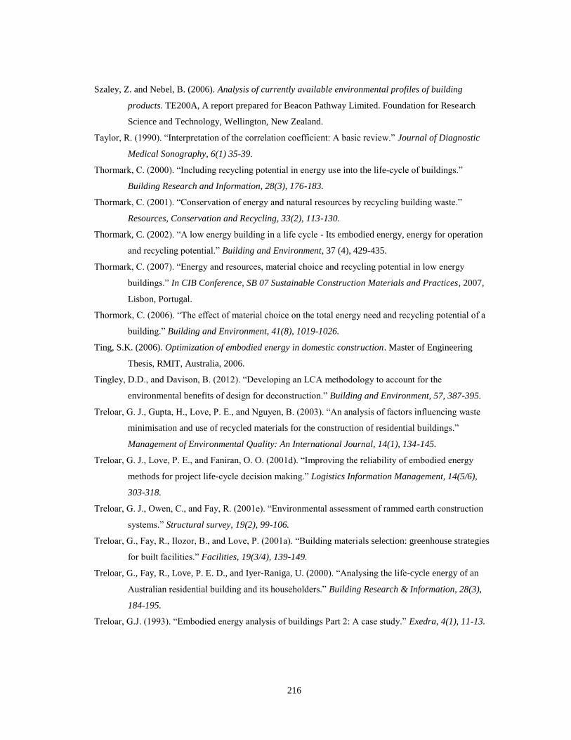
216
Szaley, Z. and Nebel, B. (2006). Analysis of currently available environmental profiles of building
products. TE200A, A report prepared for Beacon Pathway Limited. Foundation for Research
Science and Technology, Wellington, New Zealand.
Taylor, R. (1990). “Interpretation of the correlation coefficient: A basic review.” Journal of Diagnostic
Medical Sonography, 6(1) 35-39.
Thormark, C. (2000). “Including recycling potential in energy use into the life-cycle of buildings.”
Building Research and Information, 28(3), 176-183.
Thormark, C. (2001). “Conservation of energy and natural resources by recycling building waste.”
Resources, Conservation and Recycling, 33(2), 113-130.
Thormark, C. (2002). “A low energy building in a life cycle - Its embodied energy, energy for operation
and recycling potential.” Building and Environment, 37 (4), 429-435.
Thormark, C. (2007). “Energy and resources, material choice and recycling potential in low energy
buildings.” In CIB Conference, SB 07 Sustainable Construction Materials and Practices, 2007,
Lisbon, Portugal.
Thormork, C. (2006). “The effect of material choice on the total energy need and recycling potential of a
building.” Building and Environment, 41(8), 1019-1026.
Ting, S.K. (2006). Optimization of embodied energy in domestic construction. Master of Engineering
Thesis, RMIT, Australia, 2006.
Tingley, D.D., and Davison, B. (2012). “Developing an LCA methodology to account for the
environmental benefits of design for deconstruction.” Building and Environment, 57, 387-395.
Treloar, G. J., Gupta, H., Love, P. E., and Nguyen, B. (2003). “An analysis of factors influencing waste
minimisation and use of recycled materials for the construction of residential buildings.”
Management of Environmental Quality: An International Journal, 14(1), 134-145.
Treloar, G. J., Love, P. E., and Faniran, O. O. (2001d). “Improving the reliability of embodied energy
methods for project life-cycle decision making.” Logistics Information Management, 14(5/6),
303-318.
Treloar, G. J., Owen, C., and Fay, R. (2001e). “Environmental assessment of rammed earth construction
systems.” Structural survey, 19(2), 99-106.
Treloar, G., Fay, R., Ilozor, B., and Love, P. (2001a). “Building materials selection: greenhouse strategies
for built facilities.” Facilities, 19(3/4), 139-149.
Treloar, G., Fay, R., Love, P. E. D., and Iyer-Raniga, U. (2000). “Analysing the life-cycle energy of an
Australian residential building and its householders.” Building Research & Information, 28(3),
184-195.
Treloar, G.J. (1993). “Embodied energy analysis of buildings Part 2: A case study.” Exedra, 4(1), 11-13.

217
Treloar, G.J. (1997). “Extracting embodied energy paths from input-output tables: Towards an input-
output- based hybrid energy analysis method.” Economic Systems Research, 9(4), 375-391.
Treloar, G.J. (1998). A comprehensive embodied energy analysis framework. Ph.D. Thesis, Deakin
University, Victoria. Australia.
Treloar, G.J., Fay, R., Ilozor, B., and Love, P.E.D. (2001c). “An analysis of the embodied energy of office
buildings by height.” Facilities, 19(5/6), 204-214.
Treloar, G.J., Love, P.E.D. and Holt, G.D. (2001b). “Using national input output data for embodied energy
analysis of individual residential buildings.” Construction Management and Economics, 19(1),
49-61.
Treloar, G.J., McCoubrie, A., Love, P.A.D., and Iyer-Raniga, U. (1999). “Embodied energy analysis of
fixtures, fittings and furniture in office buildings.” Facilities, 17(11), 403-409.
Trusty, W. (2006). The environmental side of sustainability: Using life cycle assessment to assess true
performance. NRCC-48691, Building Science Insight 2006, Sustainable Infrastructure:
Techniques, Tools & Guidelines. National Research Council of Canada.
Ulgiati, S., Ascione, M., Bargigli, S., Cherubini, F., Federici, M., Franzese, P. P., Raugei, M., Viglia, S.,
and Zucaro, A. (2010). Multi-method and multi-scale analysis of energy and resource conversion
and use. In Barbir, F. and Ulgiati (Eds.), Energy Options Impact on Regional Security (pp. 1-36).
Springer, Netherlands.
UNDESA (2011). World Population Prospects: The 2010 Revision. POP/DB/WPP/Rev.2010/04/F01A,
June 2011. United Nations, Department of Economic and Social Affairs, Population Division.
Upadhyaya, S. (2010). Compilation of energy statistics for economic analysis. Development policy and
strategic research branch working paper 01/2010. United Nations Industrial Development
Organization, Vienna.
Upton, B., Miner, R., Spinney, M., and Heath, L. (2008). “The greenhouse gas and energy impacts of
using wood instead of alternatives in residential construction in the United States.” Biomass &
Bioenergy, 32(1), 1-10.
Ürge-Vorsatz, D., and Metz, B. (2009). “Energy efficiency: how far does it get us in controlling climate
change?” Energy Efficiency, 2(2), 87-94.
Urge-Vorsatz, D., and Novikova, A. (2006). Opportunities and costs of carbon dioxide mitigation in the
world’s domestic sector. Central European University, Budapest, Hungary.
USBEA (2008). 2002 Benchmark input-output data, 2002 data files. United States Department of
Commerce, Bureau of Economic Analysis. Retrieved from
http://www.bea.gov/industry/io_benchmark.htm#2002data
USBEA (2005). Fulltime ans part-time employees by industry. United States Department of Commerce,
Bureau of Economic Analysis. Retrieved from http://www.bea.gov/histdata/NIyear.asp

218
USBEA (2011). Fixed assets and consumer durable goods for 1997-2010. United States Bureau of
Economic Analysis. Retrieved from
http://www.bea.gov/scb/pdf/2011/09%20September/0911_fixed-assets.pdf
USBEA (2012). Fixed assets accounts tables. United States Bureau of Economic Analysis. Retrieved from
http://www.bea.gov/iTable/iTable.cfm?ReqID=10&step=1#reqid=10&step=1&isuri=1
USCB (1995). 1992 Census of Mineral Industries, Industry Series. United States Census Bureau,
Washington, D.C. Retrieved from http://www.census.gov/prod/www/economic_census.html
USCB (1999). 1997 Economic Census, Mining, Industry Series. United States Census Bureau,
Washington, D.C. Retrieved from http://www.census.gov/epcd/www/ec97stat.htm
USCB (2002a). American Community Survey Data. United States Census Bureau, Washington, D.C.
Retrieved from http://www2.census.gov/acs/downloads/Core_Tables/2002/
USCB (2002b). Current Industrial Reports Series, monthly, quarterly, and annual reports. United States
Census Bureau, Washington, D.C. Retrieved from
http://www.census.gov/manufacturing/cir/historical_data/index.html
USCB (2002c). 2002 NAICS definitions. United States Census Bureau, Washington, D.C. Retrieved from
http://www.census.gov/eos/www/naics/2002NAICS/2002_Definition_File.pdf
USCB (2002d). Annual Capital Expenditure Survey. United States Census Bureau, Washington, D.C.
Retrieved on February 22, 2013, from http://www.census.gov/econ/aces/xls/2002/
USCB (2002e). Utilities: Subject Series – Misc. Subjects: Construction Activity by Utilities for the United
States: 2002. 2002 Economic Census, United States Census Bureau, Washington, D.C. Retrieved
from
http://factfinder2.census.gov/faces/tableservices/jsf/pages/productview.xhtml?pid=ECN_2002_U
S_22SXSB4&prodType=table
USCB (2004). 2002 Economic Census, Mining, Industry Series. United States Census Bureau,
Washington, D.C. Retrieved from http://www.census.gov/econ/census02/guide/INDRPT21.HTM
USCB (2005). 2002 Economic Census, Construction, Industry Series. United States Census Bureau,
Washington, D.C. Retrieved from http://www.census.gov/econ/census02/guide/INDRPT23.HTM
USCB (2006a). Materials summary: 2002, 2002 Economic Census, Manufacturing Subject Series. EC02-
31SM-1.United States Census Bureau, Washington, D.C. Retrieved from
http://www.census.gov/prod/ec02/ec0231sm1.pdf
USCB (2006b). Business expenses: 2002, 2002 Economic Census, Industry Series. BE02-001-
1(RV).United States Census Bureau, Washington, D.C. Retrieved from
http://www.census.gov/prod/ec02/be0200i1.pdf

219
USCB (2006c). Statistical abstract of the United States: 2006, Natural resources. United States Census
Bureau, Washington, D.C. Retrieved on February 27, 2013, from
https://www.census.gov/prod/2005pubs/06statab/natresor.pdf
USCB (2007). 2007 Economic Census, Mining, Industry Series. United States Census Bureau,
Washington, D.C. Retrieved from
http://factfinder2.census.gov/faces/nav/jsf/pages/searchresults.xhtml?refresh=t
USCB (2012). New privately owned housing units authorized by building permits in permit-issuing places.
United States Census Bureau, Washington, D.C. Retrieved on 12 June, 2013 from
http://www.census.gov/construction/pdf/bpann.pdf
USCB (2013). Annual value of construction put in place 1993-2001 and 2002-2012. United States Census
Bureau, Washington, D.C. Retrieved on 12 June, 2013 from
http://www.census.gov/construction/c30/totpage.html
USDA (2002). 2002 U.S. farm and fuel expenses. Agricultural Resource Management Survey (ARMS).
Data obtained through email communication from NASS Datalab.
USDA (2004). Farm production expenditures, 2003 summary, July 2004. United States Department of
Agriculture, Washington, D.C.
USDOC (2003). Annual Survey of Manufactures: General Statistics: Capital Expenditures for Plant and
Equipment by Industry Groups and Industries: 2003 and 2002. United States Census Bureau,
Washington, D.C. Retrieved from
http://www2.census.gov/econ2003/AM/sector31/AM0331GS105.zip
USDOC (2005). Statistics for industry groups and industries: 2003, M03 (AS)-1 (RV). Annual Survey of
Manufactures, United States Department of Commerce, Economics and Statistics Division,
United States Census Bureau, Washington, D.C.
USDOE (2001). Greening federal facilities, An energy, environmental, and economic resource guide for
federal facility managers and designers. DOE/GO-102001-1165, May 2001, Office of Energy
Efficiency and Renewable Energy, Federal Energy Management Program, United States
Department of Energy, Washington, D.C.
USDOE (2007). Mining industry energy bandwidth study. June 2007, Industrial Technologies Program,
Energy Efficiency and Renewable Energy, United States Department of Energy, Washington,
D.C.
USDOE (2008). Emissions of greenhouse gases in the United States 2007. DOE/EIA-0573 (2007),
December 2008, Office of Integrated Analysis and Forecasting, United States Department of
Energy, Washington, D.C.
USDOE (2012). 2011 Building Energy Data Book. March 2012, Buildings Technologies Program, Energy
Efficiency and Renewable Energy, United States Department of Energy, Washington, D.C.
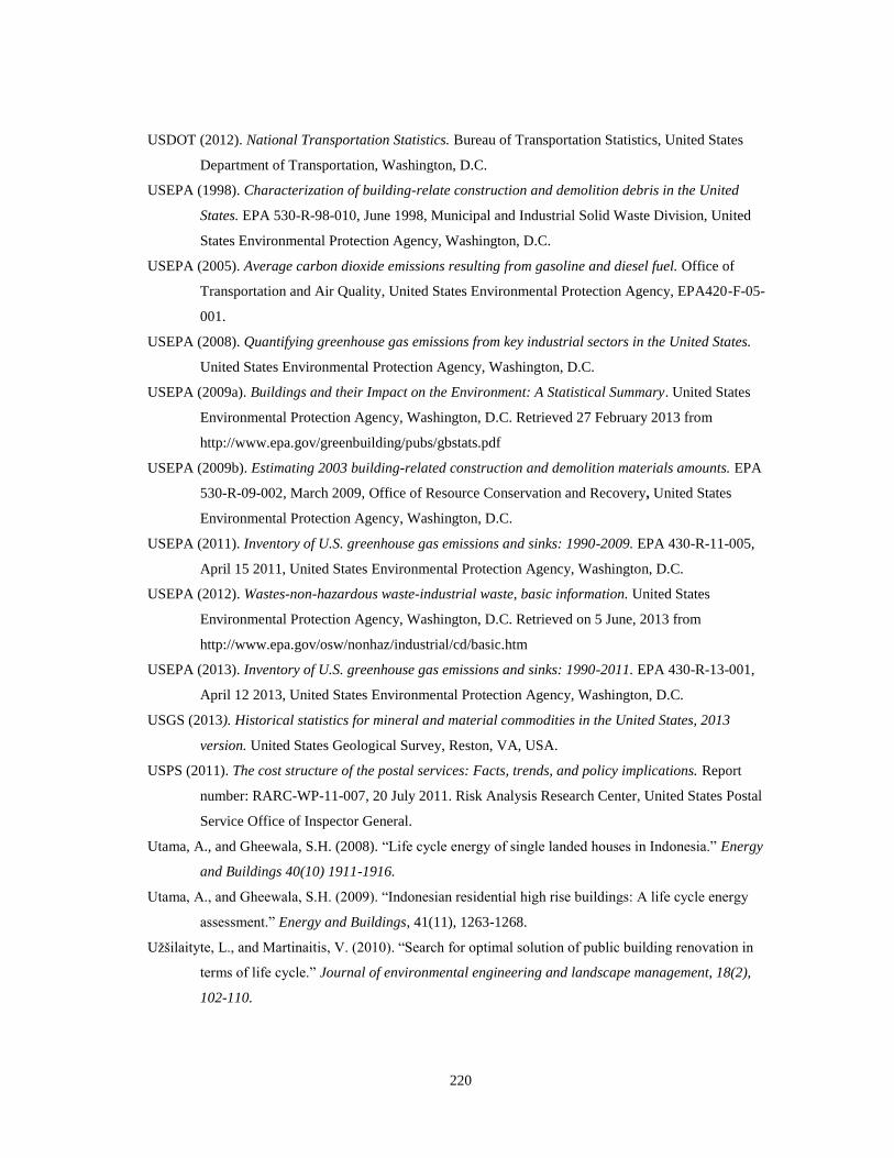
220
USDOT (2012). National Transportation Statistics. Bureau of Transportation Statistics, United States
Department of Transportation, Washington, D.C.
USEPA (1998). Characterization of building-relate construction and demolition debris in the United
States. EPA 530-R-98-010, June 1998, Municipal and Industrial Solid Waste Division, United
States Environmental Protection Agency, Washington, D.C.
USEPA (2005). Average carbon dioxide emissions resulting from gasoline and diesel fuel. Office of
Transportation and Air Quality, United States Environmental Protection Agency, EPA420-F-05-
001.
USEPA (2008). Quantifying greenhouse gas emissions from key industrial sectors in the United States.
United States Environmental Protection Agency, Washington, D.C.
USEPA (2009a). Buildings and their Impact on the Environment: A Statistical Summary. United States
Environmental Protection Agency, Washington, D.C. Retrieved 27 February 2013 from
http://www.epa.gov/greenbuilding/pubs/gbstats.pdf
USEPA (2009b). Estimating 2003 building-related construction and demolition materials amounts. EPA
530-R-09-002, March 2009, Office of Resource Conservation and Recovery, United States
Environmental Protection Agency, Washington, D.C.
USEPA (2011). Inventory of U.S. greenhouse gas emissions and sinks: 1990-2009. EPA 430-R-11-005,
April 15 2011, United States Environmental Protection Agency, Washington, D.C.
USEPA (2012). Wastes-non-hazardous waste-industrial waste, basic information. United States
Environmental Protection Agency, Washington, D.C. Retrieved on 5 June, 2013 from
http://www.epa.gov/osw/nonhaz/industrial/cd/basic.htm
USEPA (2013). Inventory of U.S. greenhouse gas emissions and sinks: 1990-2011. EPA 430-R-13-001,
April 12 2013, United States Environmental Protection Agency, Washington, D.C.
USGS (2013). Historical statistics for mineral and material commodities in the United States, 2013
version. United States Geological Survey, Reston, VA, USA.
USPS (2011). The cost structure of the postal services: Facts, trends, and policy implications. Report
number: RARC-WP-11-007, 20 July 2011. Risk Analysis Research Center, United States Postal
Service Office of Inspector General.
Utama, A., and Gheewala, S.H. (2008). “Life cycle energy of single landed houses in Indonesia.” Energy
and Buildings 40(10) 1911-1916.
Utama, A., and Gheewala, S.H. (2009). “Indonesian residential high rise buildings: A life cycle energy
assessment.” Energy and Buildings, 41(11), 1263-1268.
Užšilaityte, L., and Martinaitis, V. (2010). “Search for optimal solution of public building renovation in
terms of life cycle.” Journal of environmental engineering and landscape management, 18(2),
102-110.
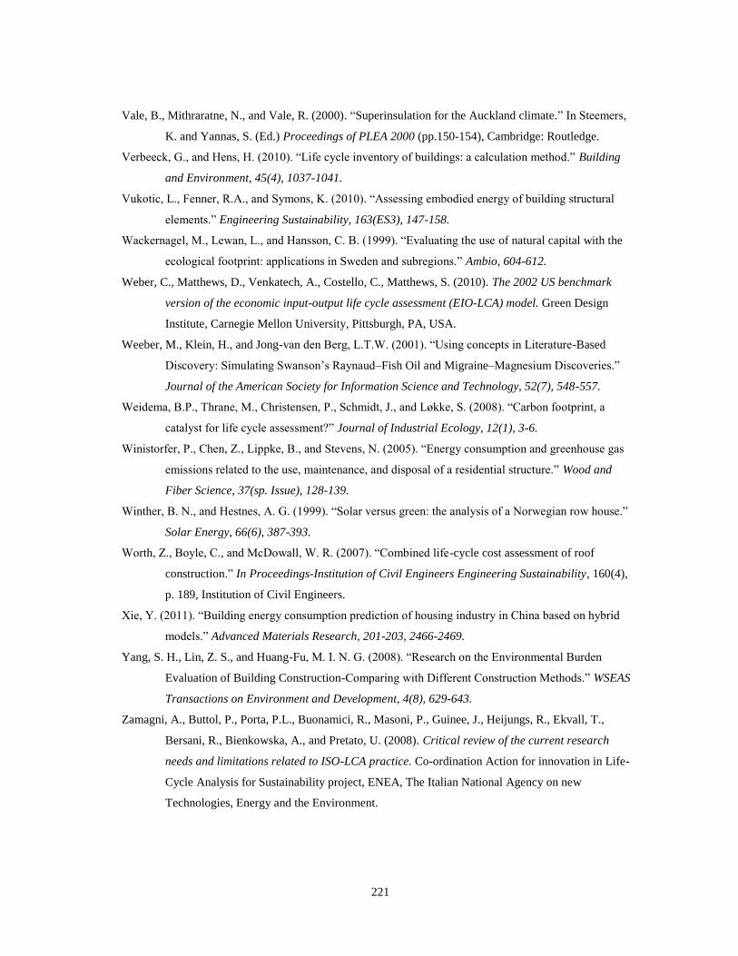
221
Vale, B., Mithraratne, N., and Vale, R. (2000). “Superinsulation for the Auckland climate.” In Steemers,
K. and Yannas, S. (Ed.) Proceedings of PLEA 2000 (pp.150-154), Cambridge: Routledge.
Verbeeck, G., and Hens, H. (2010). “Life cycle inventory of buildings: a calculation method.” Building
and Environment, 45(4), 1037-1041.
Vukotic, L., Fenner, R.A., and Symons, K. (2010). “Assessing embodied energy of building structural
elements.” Engineering Sustainability, 163(ES3), 147-158.
Wackernagel, M., Lewan, L., and Hansson, C. B. (1999). “Evaluating the use of natural capital with the
ecological footprint: applications in Sweden and subregions.” Ambio, 604-612.
Weber, C., Matthews, D., Venkatech, A., Costello, C., Matthews, S. (2010). The 2002 US benchmark
version of the economic input-output life cycle assessment (EIO-LCA) model. Green Design
Institute, Carnegie Mellon University, Pittsburgh, PA, USA.
Weeber, M., Klein, H., and Jong-van den Berg, L.T.W. (2001). “Using concepts in Literature-Based
Discovery: Simulating Swanson’s Raynaud–Fish Oil and Migraine–Magnesium Discoveries.”
Journal of the American Society for Information Science and Technology, 52(7), 548-557.
Weidema, B.P., Thrane, M., Christensen, P., Schmidt, J., and Løkke, S. (2008). “Carbon footprint, a
catalyst for life cycle assessment?” Journal of Industrial Ecology, 12(1), 3-6.
Winistorfer, P., Chen, Z., Lippke, B., and Stevens, N. (2005). “Energy consumption and greenhouse gas
emissions related to the use, maintenance, and disposal of a residential structure.” Wood and
Fiber Science, 37(sp. Issue), 128-139.
Winther, B. N., and Hestnes, A. G. (1999). “Solar versus green: the analysis of a Norwegian row house.”
Solar Energy, 66(6), 387-393.
Worth, Z., Boyle, C., and McDowall, W. R. (2007). “Combined life-cycle cost assessment of roof
construction.” In Proceedings-Institution of Civil Engineers Engineering Sustainability, 160(4),
p. 189, Institution of Civil Engineers.
Xie, Y. (2011). “Building energy consumption prediction of housing industry in China based on hybrid
models.” Advanced Materials Research, 201-203, 2466-2469.
Yang, S. H., Lin, Z. S., and Huang-Fu, M. I. N. G. (2008). “Research on the Environmental Burden
Evaluation of Building Construction-Comparing with Different Construction Methods.” WSEAS
Transactions on Environment and Development, 4(8), 629-643.
Zamagni, A., Buttol, P., Porta, P.L., Buonamici, R., Masoni, P., Guinee, J., Heijungs, R., Ekvall, T.,
Bersani, R., Bienkowska, A., and Pretato, U. (2008). Critical review of the current research
needs and limitations related to ISO-LCA practice. Co-ordination Action for innovation in Life-
Cycle Analysis for Sustainability project, ENEA, The Italian National Agency on new
Technologies, Energy and the Environment.

222
Zhu, X., Lu, Y., and Cui, Q. (2010). “Efficiency and equity implications of carbon tax in the construction
industry.” In Taylor, J.E., and Chinowsky, P. (Eds.) Engineering Project Organizations
Conference.
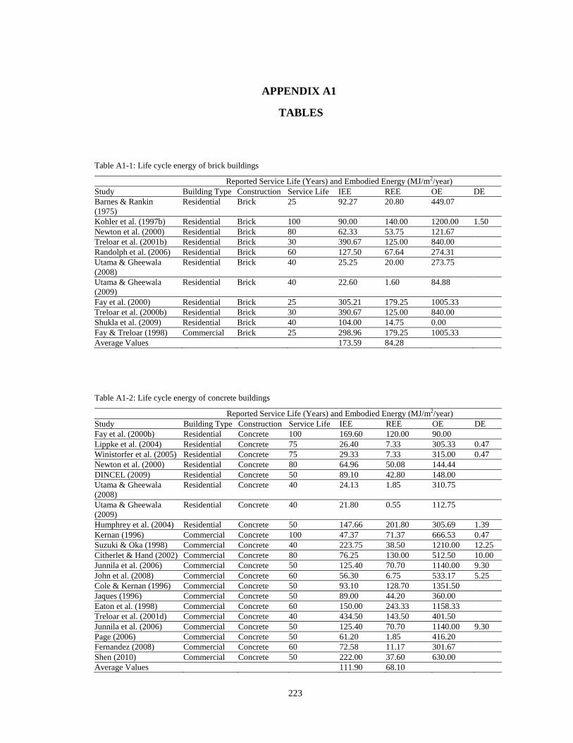
223
APPENDIX A1
TABLES
Table A1-1: Life cycle energy of brick buildings
Reported Service Life (Years) and Embodied Energy (MJ/m2/year)
Study Building Type Construction Service Life IEE REE OE DE
Barnes & Rankin
(1975)
Residential Brick 25 92.27 20.80 449.07
Kohler et al. (1997b) Residential Brick 100 90.00 140.00 1200.00 1.50
Newton et al. (2000) Residential Brick 80 62.33 53.75 121.67
Treloar et al. (2001b) Residential Brick 30 390.67 125.00 840.00
Randolph et al. (2006) Residential Brick 60 127.50 67.64 274.31
Utama & Gheewala
(2008)
Residential Brick 40 25.25 20.00 273.75
Utama & Gheewala
(2009)
Residential Brick 40 22.60 1.60 84.88
Fay et al. (2000) Residential Brick 25 305.21 179.25 1005.33
Treloar et al. (2000b) Residential Brick 30 390.67 125.00 840.00
Shukla et al. (2009) Residential Brick 40 104.00 14.75 0.00
Fay & Treloar (1998) Commercial Brick 25 298.96 179.25 1005.33
Average Values 173.59 84.28
Table A1-2: Life cycle energy of concrete buildings
Reported Service Life (Years) and Embodied Energy (MJ/m2/year)
Study Building Type Construction Service Life IEE REE OE DE
Fay et al. (2000b) Residential Concrete 100 169.60 120.00 90.00
Lippke et al. (2004) Residential Concrete 75 26.40 7.33 305.33 0.47
Winistorfer et al. (2005) Residential Concrete 75 29.33 7.33 315.00 0.47
Newton et al. (2000) Residential Concrete 80 64.96 50.08 144.44
DINCEL (2009) Residential Concrete 50 89.10 42.80 148.00
Utama & Gheewala
(2008)
Residential Concrete 40 24.13 1.85 310.75
Utama & Gheewala
(2009)
Residential Concrete 40 21.80 0.55 112.75
Humphrey et al. (2004) Residential Concrete 50 147.66 201.80 305.69 1.39
Kernan (1996) Commercial Concrete 100 47.37 71.37 666.53 0.47
Suzuki & Oka (1998) Commercial Concrete 40 223.75 38.50 1210.00 12.25
Citherlet & Hand (2002) Commercial Concrete 80 76.25 130.00 512.50 10.00
Junnila et al. (2006) Commercial Concrete 50 125.40 70.70 1140.00 9.30
John et al. (2008) Commercial Concrete 60 56.30 6.75 533.17 5.25
Cole & Kernan (1996) Commercial Concrete 50 93.10 128.70 1351.50
Jaques (1996) Commercial Concrete 50 89.00 44.20 360.00
Eaton et al. (1998) Commercial Concrete 60 150.00 243.33 1158.33
Treloar et al. (2001d) Commercial Concrete 40 434.50 143.50 401.50
Junnila et al. (2006) Commercial Concrete 50 125.40 70.70 1140.00 9.30
Page (2006) Commercial Concrete 50 61.20 1.85 416.20
Fernandez (2008) Commercial Concrete 60 72.58 11.17 301.67
Shen (2010) Commercial Concrete 50 222.00 37.60 630.00
Average Values 111.90 68.10
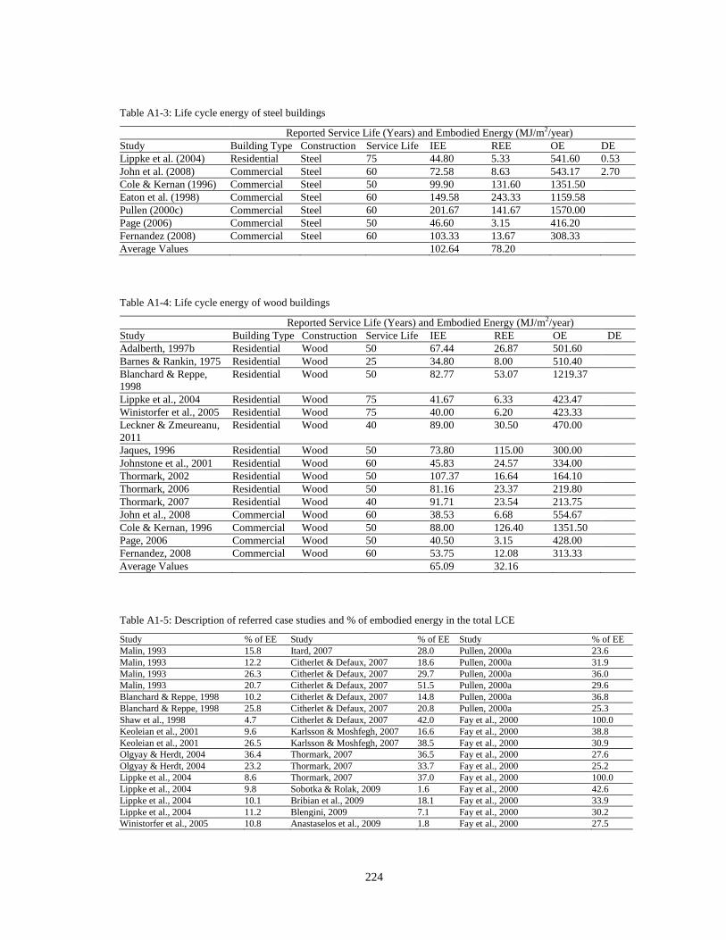
224
Table A1-3: Life cycle energy of steel buildings
Reported Service Life (Years) and Embodied Energy (MJ/m2/year)
Study Building Type Construction Service Life IEE REE OE DE
Lippke et al. (2004) Residential Steel 75 44.80 5.33 541.60 0.53
John et al. (2008) Commercial Steel 60 72.58 8.63 543.17 2.70
Cole & Kernan (1996) Commercial Steel 50 99.90 131.60 1351.50
Eaton et al. (1998) Commercial Steel 60 149.58 243.33 1159.58
Pullen (2000c) Commercial Steel 60 201.67 141.67 1570.00
Page (2006) Commercial Steel 50 46.60 3.15 416.20
Fernandez (2008) Commercial Steel 60 103.33 13.67 308.33
Average Values 102.64 78.20
Table A1-4: Life cycle energy of wood buildings
Reported Service Life (Years) and Embodied Energy (MJ/m2/year)
Study Building Type Construction Service Life IEE REE OE DE
Adalberth, 1997b Residential Wood 50 67.44 26.87 501.60
Barnes & Rankin, 1975 Residential Wood 25 34.80 8.00 510.40
Blanchard & Reppe,
1998
Residential Wood 50 82.77 53.07 1219.37
Lippke et al., 2004 Residential Wood 75 41.67 6.33 423.47
Winistorfer et al., 2005 Residential Wood 75 40.00 6.20 423.33
Leckner & Zmeureanu,
2011
Residential Wood 40 89.00 30.50 470.00
Jaques, 1996 Residential Wood 50 73.80 115.00 300.00
Johnstone et al., 2001 Residential Wood 60 45.83 24.57 334.00
Thormark, 2002 Residential Wood 50 107.37 16.64 164.10
Thormark, 2006 Residential Wood 50 81.16 23.37 219.80
Thormark, 2007 Residential Wood 40 91.71 23.54 213.75
John et al., 2008 Commercial Wood 60 38.53 6.68 554.67
Cole & Kernan, 1996 Commercial Wood 50 88.00 126.40 1351.50
Page, 2006 Commercial Wood 50 40.50 3.15 428.00
Fernandez, 2008 Commercial Wood 60 53.75 12.08 313.33
Average Values 65.09 32.16
Table A1-5: Description of referred case studies and % of embodied energy in the total LCE
Study % of EE Study % of EE Study % of EE
Malin, 1993 15.8 Itard, 2007 28.0 Pullen, 2000a 23.6
Malin, 1993 12.2 Citherlet & Defaux, 2007 18.6 Pullen, 2000a 31.9
Malin, 1993 26.3 Citherlet & Defaux, 2007 29.7 Pullen, 2000a 36.0
Malin, 1993 20.7 Citherlet & Defaux, 2007 51.5 Pullen, 2000a 29.6
Blanchard & Reppe, 1998 10.2 Citherlet & Defaux, 2007 14.8 Pullen, 2000a 36.8
Blanchard & Reppe, 1998 25.8 Citherlet & Defaux, 2007 20.8 Pullen, 2000a 25.3
Shaw et al., 1998 4.7 Citherlet & Defaux, 2007 42.0 Fay et al., 2000 100.0
Keoleian et al., 2001 9.6 Karlsson & Moshfegh, 2007 16.6 Fay et al., 2000 38.8
Keoleian et al., 2001 26.5 Karlsson & Moshfegh, 2007 38.5 Fay et al., 2000 30.9
Olgyay & Herdt, 2004 36.4 Thormark, 2007 36.5 Fay et al., 2000 27.6
Olgyay & Herdt, 2004 23.2 Thormark, 2007 33.7 Fay et al., 2000 25.2
Lippke et al., 2004 8.6 Thormark, 2007 37.0 Fay et al., 2000 100.0
Lippke et al., 2004 9.8 Sobotka & Rolak, 2009 1.6 Fay et al., 2000 42.6
Lippke et al., 2004 10.1 Bribian et al., 2009 18.1 Fay et al., 2000 33.9
Lippke et al., 2004 11.2 Blengini, 2009 7.1 Fay et al., 2000 30.2
Winistorfer et al., 2005 10.8 Anastaselos et al., 2009 1.8 Fay et al., 2000 27.5
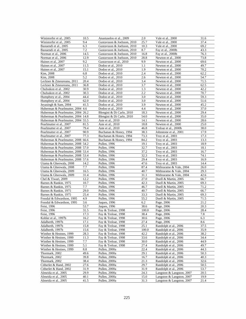
225
Winistorfer et al., 2005 10.5 Anastaselos et al., 2009 2.0 Vale et al., 2000 31.6
Winistorfer et al., 2005 9.4 Gustavsson & Joelsson, 2010 25.7 Vale et al., 2000 37.4
Baouendi et al., 2005 6.3 Gustavsson & Joelsson, 2010 10.3 Vale et al., 2000 69.2
Baouendi et al., 2005 7.2 Gustavsson & Joelsson, 2010 8.7 Fay et al., 2000b 43.3
Norman et al., 2006 14.5 Gustavsson & Joelsson, 2010 16.8 Fay et al., 2000b 76.3
Norman et al., 2006 12.9 Gustavsson & Joelsson, 2010 28.8 Newton et al., 2000 73.8
Haines et al., 2007 9.2 Gustavsson et al., 2010 9.9 Newton et al., 2000 69.6
Haines et al., 2007 11.5 Dodoo et al., 2010 1.1 Newton et al., 2000 49.7
Haines et al., 2007 15.1 Dodoo et al., 2010 1.9 Newton et al., 2000 70.2
Kim, 2008 6.8 Dodoo et al., 2010 2.4 Newton et al., 2000 62.2
Kim, 2008 5.2 Dodoo et al., 2010 2.6 Newton et al., 2000 54.7
Leckner & Zmeureanu, 2011 20.4 Dodoo et al., 2010 3.4 Newton et al., 2000 71.5
Leckner & Zmeureanu, 2011 36.8 Dodoo et al., 2010 3.7 Newton et al., 2000 62.5
Chulsukon et al., 2002 30.9 Dodoo et al., 2010 1.3 Newton et al., 2000 42.2
Chulsukon et al., 2002 30.3 Dodoo et al., 2010 2.2 Newton et al., 2000 70.7
Humphrey et al., 2004 44.4 Dodoo et al., 2010 3.0 Newton et al., 2000 59.3
Humphrey et al., 2004 62.0 Dodoo et al., 2010 3.0 Newton et al., 2000 51.6
Jeyasingh & Sam, 2004 41.5 Dodoo et al., 2010 3.9 Newton et al., 2000 45.2
Huberman & Pearlmutter, 2004 4.6 Dodoo et al., 2010 4.4 Newton et al., 2000 37.0
Huberman & Pearlmutter, 2004 26.2 Blengini & Di Carlo, 2010 18.3 Newton et al., 2000 29.4
Huberman & Pearlmutter, 2004 14.8 Blengini & Di Carlo, 2010 54.0 Newton et al., 2000 35.0
Huberman & Pearlmutter, 2004 55.5 Aste et al., 2010 14.1 Newton et al., 2000 28.6
Pearlmutter et al., 2007 81.5 Aste et al., 2010 18.8 Newton et al., 2000 25.0
Pearlmutter et al., 2007 79.4 Aste et al., 2010 46.8 Treloar et al., 2000b 38.0
Pearlmutter et al., 2007 90.9 Buchanan & Honey, 1994 38.3 Johnstone et al., 2001 17.9
Pearlmutter et al., 2007 77.3 Buchanan & Honey, 1994 73.3 Troy et al., 2003 17.3
Huberman & Pearlmutter, 2008 66.6 Buchanan & Honey, 1994 84.2 Troy et al., 2003 13.3
Huberman & Pearlmutter, 2008 54.2 Pullen, 1996 19.1 Troy et al., 2003 18.9
Huberman & Pearlmutter, 2008 57.0 Pullen, 1996 32.7 Troy et al., 2003 18.1
Huberman & Pearlmutter, 2008 53.4 Pullen, 1996 37.2 Troy et al., 2003 16.7
Huberman & Pearlmutter, 2008 53.4 Pullen, 1996 32.3 Troy et al., 2003 74.1
Huberman & Pearlmutter, 2008 57.6 Pullen, 1996 29.4 Troy et al., 2003 16.9
Utama & Gheewala, 2008 14.2 Pullen, 1996 47.6 Troy et al., 2003 14.4
Utama & Gheewala, 2008 7.7 Pullen, 1996 87.4 Mithraratne & Vale, 2004 26.0
Utama & Gheewala, 2009 16.5 Pullen, 1996 40.7 Mithraratne & Vale, 2004 29.3
Utama & Gheewala, 2009 31.4 Pullen, 1996 31.1 Mithraratne & Vale, 2004 42.6
Chel & Tiwari, 2009 12.2 Pullen, 1996 27.0 Duell & Martin, 2005 66.7
Barnes & Rankin, 1975 10.7 Pullen, 1996 42.3 Duell & Martin, 2005 69.3
Barnes & Rankin, 1975 7.7 Pullen, 1996 46.7 Duell & Martin, 2005 71.2
Barnes & Rankin, 1975 29.0 Pullen, 1996 40.7 Duell & Martin, 2005 66.7
Barnes & Rankin, 1975 25.4 Pullen, 1996 33.3 Duell & Martin, 2005 69.3
Fossdal & Edwardson, 1995 4.9 Pullen, 1996 55.2 Duell & Martin, 2005 71.5
Fossdal & Edwardson, 1995 3.6 Jaques, 1996 6.2 Page, 2006 21.2
Feist, 1996 53.7 Jaques, 1996 38.6 Page, 2006 20.3
Feist, 1996 31.5 Fay & Treloar, 1998 100.0 Page, 2006 28.4
Feist, 1996 17.3 Fay & Treloar, 1998 38.4 Page, 2006 7.8
Kohler et al., 1997b 16.2 Fay & Treloar, 1998 30.6 Page, 2006 6.3
Adalberth, 1997b 17.1 Fay & Treloar, 1998 27.4 Page, 2006 8.6
Adalberth, 1997b 15.8 Fay & Treloar, 1998 25.1 Randolph et al., 2006 37.5
Adalberth, 1997b 15.6 Fay & Treloar, 1998 100.0 Randolph et al., 2006 35.9
Winther & Hestnes, 1999 28.3 Fay & Treloar, 1998 42.2 Randolph et al., 2006 38.2
Winther & Hestnes, 1999 11.3 Fay & Treloar, 1998 33.6 Randolph et al., 2006 34.4
Winther & Hestnes, 1999 7.7 Fay & Treloar, 1998 30.0 Randolph et al., 2006 44.9
Winther & Hestnes, 1999 5.1 Fay & Treloar, 1998 27.4 Randolph et al., 2006 49.7
Winther & Hestnes, 1999 8.8 Pullen, 2000a 22.4 Randolph et al., 2006 44.3
Thormark, 2002 49.6 Pullen, 2000a 29.1 Randolph et al., 2006 50.3
Thormark, 2002 39.8 Pullen, 2000a 16.7 Randolph et al., 2006 40.3
Thormark, 2002 38.4 Pullen, 2000a 21.3 Randolph et al., 2006 32.6
Citherlet & Hand, 2002 27.6 Pullen, 2000a 29.7 Randolph et al., 2006 50.5
Citherlet & Hand, 2002 31.9 Pullen, 2000a 31.9 Randolph et al., 2006 53.7
Almeida et al., 2005 29.9 Pullen, 2000a 24.3 Langston & Langston, 2007 20.5
Almeida et al., 2005 40.1 Pullen, 2000a 15.0 Langston & Langston, 2007 19.9
Almeida et al., 2005 41.5 Pullen, 2000a 31.3 Langston & Langston, 2007 21.4
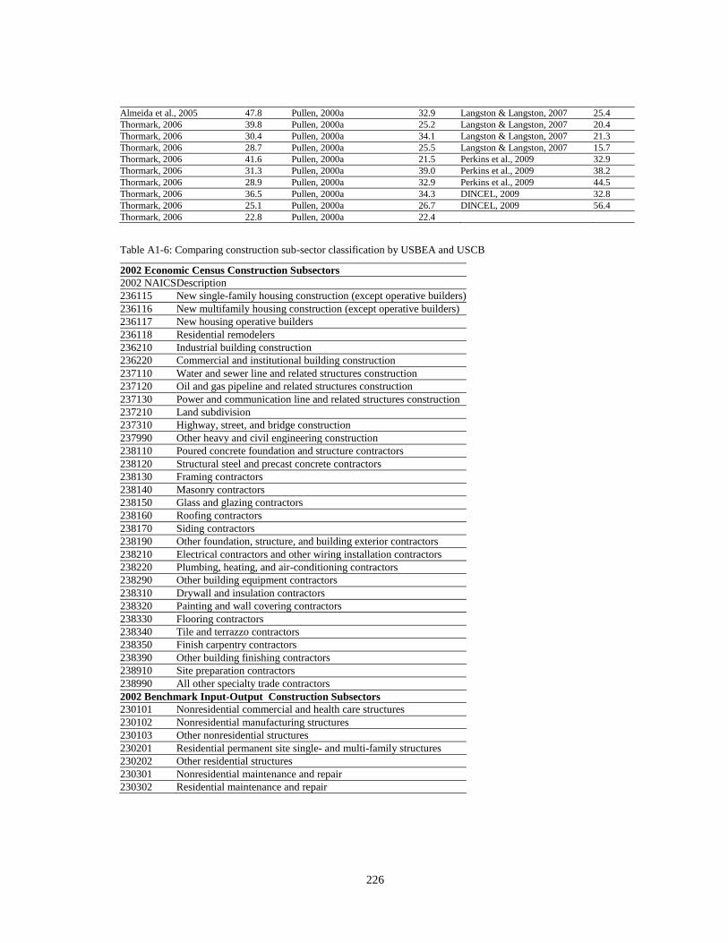
226
Almeida et al., 2005 47.8 Pullen, 2000a 32.9 Langston & Langston, 2007 25.4
Thormark, 2006 39.8 Pullen, 2000a 25.2 Langston & Langston, 2007 20.4
Thormark, 2006 30.4 Pullen, 2000a 34.1 Langston & Langston, 2007 21.3
Thormark, 2006 28.7 Pullen, 2000a 25.5 Langston & Langston, 2007 15.7
Thormark, 2006 41.6 Pullen, 2000a 21.5 Perkins et al., 2009 32.9
Thormark, 2006 31.3 Pullen, 2000a 39.0 Perkins et al., 2009 38.2
Thormark, 2006 28.9 Pullen, 2000a 32.9 Perkins et al., 2009 44.5
Thormark, 2006 36.5 Pullen, 2000a 34.3 DINCEL, 2009 32.8
Thormark, 2006 25.1 Pullen, 2000a 26.7 DINCEL, 2009 56.4
Thormark, 2006 22.8 Pullen, 2000a 22.4
Table A1-6: Comparing construction sub-sector classification by USBEA and USCB
2002 Economic Census Construction Subsectors
2002 NAICS Description
236115 New single-family housing construction (except operative builders)
236116 New multifamily housing construction (except operative builders)
236117 New housing operative builders
236118 Residential remodelers
236210 Industrial building construction
236220 Commercial and institutional building construction
237110 Water and sewer line and related structures construction
237120 Oil and gas pipeline and related structures construction
237130 Power and communication line and related structures construction
237210 Land subdivision
237310 Highway, street, and bridge construction
237990 Other heavy and civil engineering construction
238110 Poured concrete foundation and structure contractors
238120 Structural steel and precast concrete contractors
238130 Framing contractors
238140 Masonry contractors
238150 Glass and glazing contractors
238160 Roofing contractors
238170 Siding contractors
238190 Other foundation, structure, and building exterior contractors
238210 Electrical contractors and other wiring installation contractors
238220 Plumbing, heating, and air-conditioning contractors
238290 Other building equipment contractors
238310 Drywall and insulation contractors
238320 Painting and wall covering contractors
238330 Flooring contractors
238340 Tile and terrazzo contractors
238350 Finish carpentry contractors
238390 Other building finishing contractors
238910 Site preparation contractors
238990 All other specialty trade contractors
2002 Benchmark Input-Output Construction Subsectors
230101 Nonresidential commercial and health care structures
230102 Nonresidential manufacturing structures
230103 Other nonresidential structures
230201 Residential permanent site single- and multi-family structures
230202 Other residential structures
230301 Nonresidential maintenance and repair
230302 Residential maintenance and repair

227
Table A1-7: Service sectors and major service activities
NAICS Sector Description Activities
51 Information Creating, processing, and distributing or transmitting the information and
cultural products and rendering related services. Products and services
include print and electronic media such as newspapers, magazines,
periodicals, books, directories, music, sound recording, movies, other
videos, videography, software, broadcasting, internet publishing,
telecommunication, internet services, data processing services, libraries, and
other information services.
52 Finance and insurance Financial transactions such as creating, liquidating, and modifying
ownership status of financial assets. Included are establishments such as
central and other banks, lending establishments (e.g., credit unions,
mortgage & real estate loans, credit card companies), securities, commodity
contract establishments, insurance companies, and other related industries.
53 Real Estate, and Rental and
Leasing
Renting, leasing, and selling tangible and intangible assets for others (e.g.,
clients) and rendering related services. Included in this sector are
establishments such as lesser, real estate agents, brokers, real estate
appraisers, and rental and leasing agencies.
54 Professional, Scientific, and
Technical Services
Providing professional, scientific, and technical services such as legal;
accounting, bookkeeping, and payroll; architectural, engineering, and
related; other specialized design services; computer design; management,
scientific, and technical consulting; research and development; advertising
and related services; and other similar services.
55 Management of Companies and
Enterprises
Include establishments such as equity holders and those who oversee,
manage, or administer a company or a portfolio of companies of a
government or non-government organization.
56 Administrative and Support, and
Waste
Management and Remediation
Services
Administering and supporting routine operations of various organizations
(e.g., facilities, employment, business, travel, investigation, security,
building support and management). Also included are establishments
engaged in waste collection, sorting, treatment, and disposal and waste
remediation services.
61 Educational Services Providing education by instruction and training in a variety of disciplines.
Included are schools, junior colleges, professional schools, community
colleges, and universities.
62 Healthcare and Social Assistance Establishments such as health practitioners, clinics, hospitals, nursing
homes, medical & diagnostic laboratories, blood banks, ambulance services,
child & youth services, elderly care services, community food services, and
child daycare centers providing healthcare and social assistance.
71 Arts, Entertainment, and
Recreation
Establishments producing, organizing, promoting, or participating in live
events or exhibits. Also included are establishments operating and
maintaining facilities to exhibit objects and sites of historical, cultural, or
educational importance. Other leisure, recreational, cultural, or hobby-
related organizations are also covered in this sector. Museums, historical
sites, sports arena, theaters, performing art centers, racetracks, zoos,
botanical gardens, theme parks, nature parks, casinos, golf courses, country
clubs, skiing facilities, marinas, bowling centers, fitness centers, and similar
establishments.
72 Accommodation and Food
Services
Providing accommodation and or food and beverages for immediate
consumption. Included are hotels, motels, bed-and-breakfast inns, RV parks,
restaurants, cafeterias, bars & drinking places, caterers, and mobile eating
joints.
81 Other Services (except Public
Administration)
Providing services not covered under other service sectors. Services such as
equipment and machinery repair and maintenance; religious activities
promotion and administration; advocacy; grant-making; dry-cleaning and
laundries, personal care; death care; pet care; dating, and other similar
services.

228
Table A1-8: Regression analysis results for cost and input-output-based hybrid results with human and capital inputs
SUMMARY OUTPUT Cost & IO-Based Hybrid with Human & Capital Inputs
Regression Statistics
Multiple R 0.917937
R Square 0.842608
Adjusted R
Square
0.792608
Standard Error 29.02843
Observations 21
ANOVA
df SS MS F Significance
F
Regression 1 90223.58 90223.5
8
107.071
3
3.03E-09
Residual 20 16853 842.649
8
Total 21 107076.6
Coefficient
s
Standard
Error
t Stat P-value Lower 95% Upper
95%
Lower
95.0%
Upper
95.0%
Intercept 0 #N/A #N/A #N/A #N/A #N/A #N/A #N/A
X Variable 1 36.3167 3.509699 10.3475
2
1.78E-
09
28.99559 43.6378 28.99559 43.6378
Table A1-9: Regression analysis results for cost and input-output-based hybrid results after sector disaggregation
SUMMARY OUTPUT Cost & IO-Based Hybrid with Human & Capital Inputs After Disaggregation
Regression Statistics
Multiple R 0.913238
R Square 0.834004
Adjusted R
Square
0.784004
Standard Error 29.96184
Observations 21
ANOVA
df SS MS F Significance
F
Regression 1 90206.28 90206.2
8
100.484
7
5.06E-09
Residual 20 17954.23 897.711
7
Total 21 108160.5
Coefficient
s
Standard
Error
t Stat P-value Lower 95% Upper
95%
Lower
95.0%
Upper
95.0%
Intercept 0 #N/A #N/A #N/A #N/A #N/A #N/A #N/A
X Variable 1 36.31322 3.622553 10.0242
1
3.04E-
09
28.7567 43.86973 28.7567 43.86973

229
Table A1-10: Regression analysis results for price and input-output-based hybrid results with human and capital inputs
SUMMARY OUTPUT Price & Input-output-based Hybrid with Human & Capital Inputs
Regression Statistics
Multiple R 0.973701
R Square 0.948093
Adjusted R
Square
0.898093
Standard Error 14.61958
Observations 21
ANOVA
df SS MS F Significance
F
Regression 1 78076.82 78076.8
2
365.302
2
7.25E-14
Residual 20 4274.643 213.732
1
Total 21 82351.46
Coefficient
s
Standard
Error
t Stat P-value Lower 95% Upper
95%
Lower
95.0%
Upper
95.0%
Intercept 0 #N/A #N/A #N/A #N/A #N/A #N/A #N/A
X Variable 1 34.44825 1.802358 19.1128
8
2.56E-
14
30.6886 38.2079 30.6886 38.2079
Table A1-11: Regression analysis results for price and input-output-based hybrid results after sector disaggregation
SUMMARY OUTPUT Price & Input-output-based Hybrid with Human & Capital Inputs After
Disaggregation
Regression Statistics
Multiple R 0.971943
R Square 0.944673
Adjusted R
Square
0.894673
Standard Error 15.09479
Observations 21
ANOVA
df SS MS F Significance
F
Regression 1 77809.47 77809.4
7
341.490
3
1.33E-13
Residual 20 4557.053 227.852
7
Total 21 82366.53
Coefficient
s
Standard
Error
t Stat P-value Lower 95% Upper
95%
Lower
95.0%
Upper
95.0%
Intercept 0 #N/A #N/A #N/A #N/A #N/A #N/A #N/A
X Variable 1 34.38922 1.860943 18.4794
6
4.86E-
14
30.50736 38.27108 30.50736 38.27108
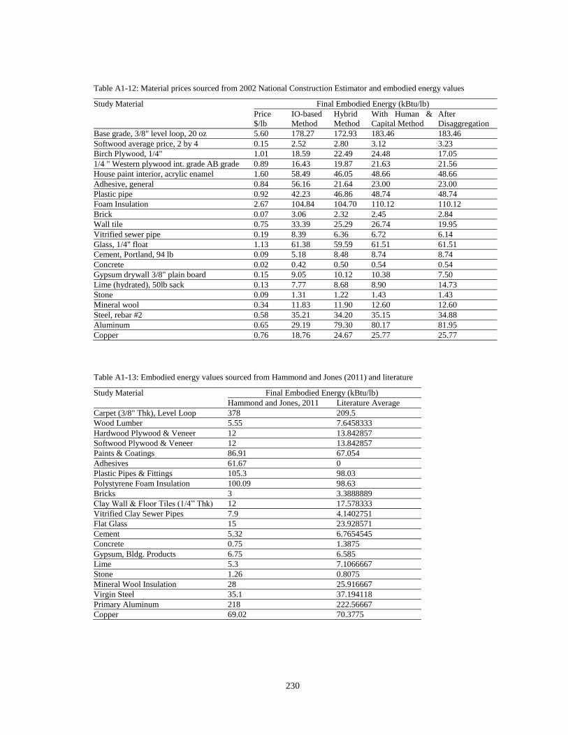
230
Table A1-12: Material prices sourced from 2002 National Construction Estimator and embodied energy values
Study Material Final Embodied Energy (kBtu/lb)
Price
$/lb
IO-based
Method
Hybrid
Method
With Human &
Capital Method
After
Disaggregation
Base grade, 3/8" level loop, 20 oz 5.60 178.27 172.93 183.46 183.46
Softwood average price, 2 by 4 0.15 2.52 2.80 3.12 3.23
Birch Plywood, 1/4" 1.01 18.59 22.49 24.48 17.05
1/4 " Western plywood int. grade AB grade 0.89 16.43 19.87 21.63 21.56
House paint interior, acrylic enamel 1.60 58.49 46.05 48.66 48.66
Adhesive, general 0.84 56.16 21.64 23.00 23.00
Plastic pipe 0.92 42.23 46.86 48.74 48.74
Foam Insulation 2.67 104.84 104.70 110.12 110.12
Brick 0.07 3.06 2.32 2.45 2.84
Wall tile 0.75 33.39 25.29 26.74 19.95
Vitrified sewer pipe 0.19 8.39 6.36 6.72 6.14
Glass, 1/4" float 1.13 61.38 59.59 61.51 61.51
Cement, Portland, 94 lb 0.09 5.18 8.48 8.74 8.74
Concrete 0.02 0.42 0.50 0.54 0.54
Gypsum drywall 3/8" plain board 0.15 9.05 10.12 10.38 7.50
Lime (hydrated), 50lb sack 0.13 7.77 8.68 8.90 14.73
Stone 0.09 1.31 1.22 1.43 1.43
Mineral wool 0.34 11.83 11.90 12.60 12.60
Steel, rebar #2 0.58 35.21 34.20 35.15 34.88
Aluminum 0.65 29.19 79.30 80.17 81.95
Copper 0.76 18.76 24.67 25.77 25.77
Table A1-13: Embodied energy values sourced from Hammond and Jones (2011) and literature
Study Material Final Embodied Energy (kBtu/lb)
Hammond and Jones, 2011 Literature Average
Carpet (3/8" Thk), Level Loop 378 209.5
Wood Lumber 5.55 7.6458333
Hardwood Plywood & Veneer 12 13.842857
Softwood Plywood & Veneer 12 13.842857
Paints & Coatings 86.91 67.054
Adhesives 61.67 0
Plastic Pipes & Fittings 105.3 98.03
Polystyrene Foam Insulation 100.09 98.63
Bricks 3 3.3888889
Clay Wall & Floor Tiles (1/4” Thk) 12 17.578333
Vitrified Clay Sewer Pipes 7.9 4.1402751
Flat Glass 15 23.928571
Cement 5.32 6.7654545
Concrete 0.75 1.3875
Gypsum, Bldg. Products 6.75 6.585
Lime 5.3 7.1066667
Stone 1.26 0.8075
Mineral Wool Insulation 28 25.916667
Virgin Steel 35.1 37.194118
Primary Aluminum 218 222.56667
Copper 69.02 70.3775
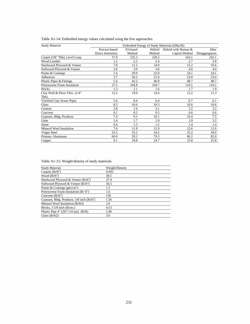
231
Table A1-14: Embodied energy values calculated using the five approaches
Study Material Embodied Energy of Study Materials (kBtu/lb)
Process-based
Direct Intensities
IO-based
Method
Hybrid
Method
Hybrid with Human &
Capital Method
After
Disaggregation
Carpet (3/8" Thk), Level Loop 37.9 235.3 228.2 242.1 242.1
Wood Lumber 1.2 2.2 2.4 2.7 2.8
Hardwood Plywood & Veneer 7.8 11.5 14.0 15.2 10.6
Softwood Plywood & Veneer 2.0 3.0 3.6 4.0 4.0
Paints & Coatings 1.6 29.0 22.8 24.1 24.1
Adhesives 3.7 56.2 21.6 23.0 23.0
Plastic Pipes & Fittings 5.6 42.2 46.9 48.7 48.7
Polystyrene Foam Insulation 27.5 104.8 104.7 110.1 110.1
Bricks 1.3 2.1 1.6 1.7 1.9
Clay Wall & Floor Tiles (1/4"
Thk)
12.2 19.0 14.4 15.2 11.3
Vitrified Clay Sewer Pipes 5.4 8.4 6.4 6.7 6.1
Glass 8.2 10.6 10.3 10.6 10.6
Cement 2.8 1.9 3.1 3.2 3.2
Concrete 0.1 0.5 0.5 0.6 0.6
Gypsum, Bldg. Products 7.4 9.1 10.1 10.4 7.5
Lime 1.4 1.7 1.9 1.9 3.2
Stone 0.4 1.3 1.2 1.4 1.4
Mineral Wool Insulation 7.6 11.8 11.9 12.6 12.6
Virgin Steel 23.3 35.2 34.2 35.2 34.9
Primary Aluminum 60.0 29.2 79.3 80.2 82.0
Copper 9.1 18.8 24.7 25.8 25.8
Table A1-15: Weight/density of study materials
Study Material Weight/Density
Carpets (lb/ft2) 0.093
Wood (lb/ft3) 38.5
Hardwood Plywood & Veneer (lb/ft3) 37.4
Softwood Plywood & Veneer (lb/ft3) 36.5
Paints & Coatings (gm/cm3) 1.5
Polystyrene Foam Insulation (lb/ ft3) 1.6
Concrete (lb/ft3) 150
Gypsum, Bldg. Products, 3/8 inch (lb/ft2) 1.56
Mineral Wool Insulation (lb/ft3) 2.0
Bricks, 3 5/8 inch (lb/no.) 4.53
Plastic Pipe 4" (267-110 psi) (lb/ft) 2.46
Glass (lb/ft2) 3.0
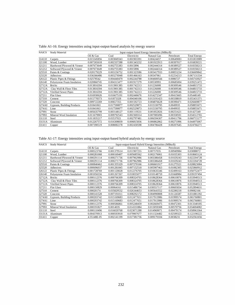
232
Table A1-16: Energy intensities using input-output-based analysis by energy source
NAICS Study Material Input-output-based Energy Intensities (MBtu/$)
Oil & Gas Coal Electricity Natural Gas Petroleum Total Energy
314110 Carpets 0.015345856 0.003849343 0.001903391 0.00424457 0.00649083 0.031833989
321100 Wood, Lumber 0.007265618 0.002337288 0.001343232 0.001922913 0.00397017 0.016839221
321211 Hardwood Plywood & Veneer 0.007673649 0.002755383 0.0015896 0.002444314 0.00389527 0.018358213
321212 Softwood Plywood & Veneer 0.007673649 0.002755383 0.0015896 0.002444314 0.00389527 0.018358213
325510 Paints & Coatings 0.020179229 0.003156752 0.001323586 0.003417933 0.00853234 0.036609842
325520 Adhesives 0.036366486 0.003276948 0.001466163 0.00347961 0.02254213 0.067131334
326122 Plastic Pipes & Fittings 0.02578542 0.004440479 0.002244788 0.004600544 0.0086727 0.045743927
326140 Polystyrene Foam Insulation 0.020860745 0.004313477 0.001917279 0.00530993 0.00685004 0.039251472
32712A Bricks 0.013816594 0.013901385 0.001742213 0.01226008 0.00309546 0.044815733
32712A Clay Wall & Floor Tiles 0.013816594 0.013901385 0.001742213 0.01226008 0.00309546 0.044815733
32712A Vitrified Sewer Pipes 0.013816594 0.013901385 0.001742213 0.01226008 0.00309546 0.044815733
327211 Flat Glass 0.016930626 0.016675191 0.002446676 0.014272347 0.00415665 0.05448149
327310 Cement 0.015778373 0.01873328 0.004340106 0.013191423 0.00338819 0.055431371
327320 Concrete 0.009722269 0.00657355 0.001592723 0.004876628 0.00390471 0.026669877
3274A0 Gypsum, Building Products 0.01841063 0.017590877 0.002529873 0.015330795 0.0049935 0.058855671
3274A1 Lime 0.01841063 0.017590877 0.002529873 0.015330795 0.0049935 0.058855671
327991 Stone 0.005635799 0.003148127 0.001119531 0.001852826 0.00251621 0.01427249
327993 Mineral Wool Insulation 0.011679903 0.009792543 0.002369314 0.007085096 0.00358591 0.034512765
331110 Steel 0.011835217 0.03537021 0.002797481 0.006594307 0.00411796 0.060715177
33131A Aluminum 0.012267572 0.016308839 0.006815836 0.006862862 0.00271996 0.044975067
331411 Copper 0.007390519 0.008082278 0.002430598 0.004786428 0.00207645 0.024766271
Table A1-17: Energy intensities using input-output-based hybrid analysis by energy source
NAICS Study Material Input-output-based Hybrid Energy Intensities (MBtu/$)
Oil & Gas Coal Electricity Natural Gas Petroleum Total Energy
314110 Carpets 0.000523766 0.001379514 0.011907255 0.00757035 0.00949984 0.03088072
321100 Wood, Lumber 0.000281068 0.000169407 0.005685562 0.002176061 0.01035303 0.018665124
321211 Hardwood Plywood & Veneer 0.000291114 0.000271736 0.007962986 0.003386458 0.01029243 0.022204728
321212 Softwood Plywood & Veneer 0.000291114 0.000271736 0.007962986 0.003386458 0.01029243 0.022204728
325510 Paints & Coatings 0.000840462 0.001355329 0.007270166 0.006601917 0.01275521 0.028823084
325520 Adhesives 0.000696037 0.001281845 0.007152518 0.005907463 0.01082305 0.025860912
326122 Plastic Pipes & Fittings 0.001728769 0.001120028 0.012276705 0.010635346 0.02499163 0.050752477
326140 Polystyrene Foam Insulation 0.001056556 0.001267267 0.010035077 0.010148759 0.01668984 0.039197494
32712A Bricks 0.000112376 0.000766309 0.008324705 0.018628364 0.00610876 0.033940513
32712A Clay Wall & Floor Tiles 0.000112376 0.000766309 0.008324705 0.018628364 0.00610876 0.033940513
32712A Vitrified Sewer Pipes 0.000112376 0.000766309 0.008324705 0.018628364 0.00610876 0.033940513
327211 Flat Glass 0.000150829 0.00064161 0.015486734 0.030557117 0.00605834 0.052894631
327310 Cement 0.00020174 0.035829532 0.026344653 0.005643552 0.02280218 0.09082166
327320 Concrete 0.000141528 0.007191011 0.008292172 0.004990808 0.01126587 0.031881392
3274A0 Gypsum, Building Products 0.000203742 0.015169683 0.012477651 0.017913986 0.01999574 0.065760801
3274A1 Lime 0.000203742 0.015169683 0.012477651 0.017913986 0.01999574 0.065760801
327991 Stone 0.000112376 0.000586861 0.005248459 0.002669475 0.00472301 0.013340185
327993 Mineral Wool Insulation 0.000191827 0.0014035 0.014331884 0.013059308 0.00570756 0.034694082
331110 Steel 0.000110496 0.016020768 0.023071288 0.014969071 0.00479174 0.058963364
33131A Aluminum 0.004370913 0.000593918 0.079907677 0.011324482 0.02599323 0.122190222
331411 Copper 4.55148E-05 0.002141199 0.017381736 0.009170104 0.0038231 0.032561656
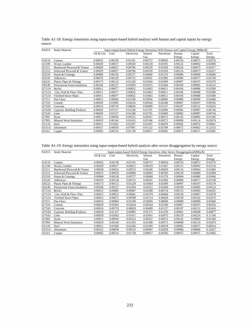
233
Table A1-18: Energy intensities using input-output-based hybrid analysis with human and capital inputs by energy
source
NAICS Study Material Input-output-based Hybrid Energy Intensities With Human and Capital Energy (MBtu/$)
Oil & Gas Coal Electricity Natural
Gas
Petroleum Human
Energy
Capital
Energy
Total
Energy
314110 Carpets 0.00052 0.00138 0.01191 0.00757 0.00950 0.00116 0.00072 0.03276
321100 Wood, Lumber 0.00028 0.00017 0.00569 0.00218 0.01035 0.00122 0.00092 0.02080
321211 Hardwood Plywood & Veneer 0.00029 0.00027 0.00796 0.00339 0.01029 0.00124 0.00073 0.02417
321212 Softwood Plywood & Veneer 0.00029 0.00027 0.00796 0.00339 0.01029 0.00124 0.00073 0.02417
325510 Paints & Coatings 0.00084 0.00136 0.00727 0.00660 0.01276 0.00084 0.00080 0.03046
325520 Adhesives 0.00070 0.00128 0.00715 0.00591 0.01082 0.00086 0.00077 0.02749
326122 Plastic Pipes & Fittings 0.00173 0.00112 0.01228 0.01064 0.02499 0.00097 0.00107 0.05279
326140 Polystyrene Foam Insulation 0.00106 0.00127 0.01004 0.01015 0.01669 0.00108 0.00095 0.04123
32712A Bricks 0.00011 0.00077 0.00832 0.01863 0.00611 0.00106 0.00088 0.03589
32712A Clay Wall & Floor Tiles 0.00011 0.00077 0.00832 0.01863 0.00611 0.00106 0.00088 0.03589
32712A Vitrified Sewer Pipes 0.00011 0.00077 0.00832 0.01863 0.00611 0.00106 0.00088 0.03589
327211 Flat Glass 0.00015 0.00064 0.01549 0.03056 0.00606 0.00080 0.00090 0.05460
327310 Cement 0.00020 0.03583 0.02634 0.00564 0.02280 0.00067 0.00207 0.09356
327320 Concrete 0.00014 0.00719 0.00829 0.00499 0.01127 0.00107 0.00121 0.03416
3274A0 Gypsum, Building Products 0.00020 0.01517 0.01248 0.01791 0.02000 0.00082 0.00087 0.06744
3274A1 Lime 0.00020 0.01517 0.01248 0.01791 0.02000 0.00082 0.00087 0.06744
327991 Stone 0.00011 0.00059 0.00525 0.00267 0.00472 0.00145 0.00082 0.01560
327993 Mineral Wool Insulation 0.00019 0.00140 0.01433 0.01306 0.00571 0.00090 0.00114 0.03674
331110 Steel 0.00011 0.01602 0.02307 0.01497 0.00479 0.00092 0.00072 0.06061
33131A Aluminum 0.00437 0.00059 0.07991 0.01132 0.02599 0.00072 0.00062 0.12353
331411 Copper 0.00005 0.00214 0.01738 0.00917 0.00382 0.00075 0.00071 0.03402
Table A1-19: Energy intensities using input-output-based hybrid analysis after sector disaggregation by energy source
NAICS Study Material Input-output-based Hybrid Energy Intensities After Sector Disaggregation(MBtu/$)
Oil & Gas Coal Electricity Natural
Gas
Petroleum Human
Energy
Capital
Energy
Total
Energy
314110 Carpets 0.00052 0.00138 0.01191 0.00757 0.00950 0.00116 0.00072 0.03276
321100 Wood, Lumber 0.00029 0.00017 0.00612 0.00218 0.01067 0.00121 0.00092 0.02156
321211 Hardwood Plywood & Veneer 0.00028 0.00016 0.00553 0.00246 0.00659 0.00116 0.00064 0.01683
321212 Softwood Plywood & Veneer 0.00015 0.00018 0.00980 0.00402 0.00783 0.00130 0.00080 0.02409
325510 Paints & Coatings 0.00084 0.00136 0.00727 0.00660 0.01276 0.00084 0.00080 0.03046
325520 Adhesives 0.00070 0.00128 0.00715 0.00591 0.01082 0.00086 0.00077 0.02749
326122 Plastic Pipes & Fittings 0.00173 0.00112 0.01228 0.01064 0.02499 0.00097 0.00107 0.05279
326140 Polystyrene Foam Insulation 0.00106 0.00127 0.01004 0.01015 0.01669 0.00108 0.00095 0.04123
32712A Bricks 0.00012 0.00085 0.00847 0.02286 0.00716 0.00123 0.00092 0.04161
32712A Clay Wall & Floor Tiles 0.00012 0.00053 0.00841 0.01079 0.00460 0.00134 0.00097 0.02678
32712A Vitrified Sewer Pipes 0.00012 0.00071 0.00598 0.01714 0.00628 0.00150 0.00102 0.03276
327211 Flat Glass 0.00015 0.00064 0.01549 0.03056 0.00606 0.00080 0.00090 0.05460
327310 Cement 0.00020 0.03583 0.02634 0.00564 0.02280 0.00067 0.00207 0.09356
327320 Concrete 0.00014 0.00719 0.00829 0.00499 0.01127 0.00107 0.00121 0.03416
3274A0 Gypsum, Building Products 0.00018 0.01157 0.00985 0.01371 0.01239 0.00061 0.00048 0.04877
3274A1 Lime 0.00028 0.02663 0.01911 0.03041 0.03075 0.00219 0.00224 0.11160
327991 Stone 0.00011 0.00059 0.00525 0.00267 0.00472 0.00145 0.00082 0.01560
327993 Mineral Wool Insulation 0.00019 0.00140 0.01433 0.01306 0.00571 0.00090 0.00114 0.03674
331110 Steel 0.00011 0.01600 0.02266 0.01495 0.00478 0.00092 0.00071 0.06014
33131A Aluminum 0.00331 0.00038 0.09133 0.00947 0.02028 0.00084 0.00066 0.12627
331411 Copper 0.00005 0.00214 0.01738 0.00917 0.00382 0.00075 0.00071 0.03402
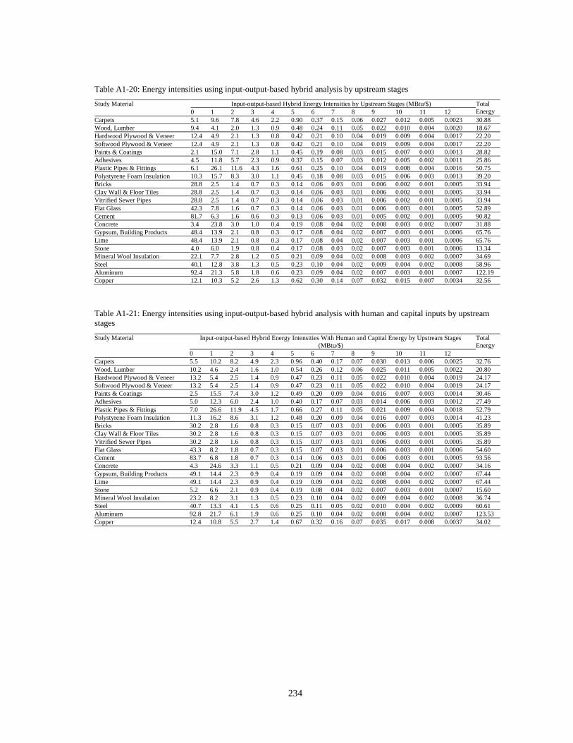
234
Table A1-20: Energy intensities using input-output-based hybrid analysis by upstream stages
Study Material Input-output-based Hybrid Energy Intensities by Upstream Stages (MBtu/$) Total
Energy 0 1 2 3 4 5 6 7 8 9 10 11 12
Carpets 5.1 9.6 7.8 4.6 2.2 0.90 0.37 0.15 0.06 0.027 0.012 0.005 0.0023 30.88
Wood, Lumber 9.4 4.1 2.0 1.3 0.9 0.48 0.24 0.11 0.05 0.022 0.010 0.004 0.0020 18.67
Hardwood Plywood & Veneer 12.4 4.9 2.1 1.3 0.8 0.42 0.21 0.10 0.04 0.019 0.009 0.004 0.0017 22.20
Softwood Plywood & Veneer 12.4 4.9 2.1 1.3 0.8 0.42 0.21 0.10 0.04 0.019 0.009 0.004 0.0017 22.20
Paints & Coatings 2.1 15.0 7.1 2.8 1.1 0.45 0.19 0.08 0.03 0.015 0.007 0.003 0.0013 28.82
Adhesives 4.5 11.8 5.7 2.3 0.9 0.37 0.15 0.07 0.03 0.012 0.005 0.002 0.0011 25.86
Plastic Pipes & Fittings 6.1 26.1 11.6 4.3 1.6 0.61 0.25 0.10 0.04 0.019 0.008 0.004 0.0016 50.75
Polystyrene Foam Insulation 10.3 15.7 8.3 3.0 1.1 0.45 0.18 0.08 0.03 0.015 0.006 0.003 0.0013 39.20
Bricks 28.8 2.5 1.4 0.7 0.3 0.14 0.06 0.03 0.01 0.006 0.002 0.001 0.0005 33.94
Clay Wall & Floor Tiles 28.8 2.5 1.4 0.7 0.3 0.14 0.06 0.03 0.01 0.006 0.002 0.001 0.0005 33.94
Vitrified Sewer Pipes 28.8 2.5 1.4 0.7 0.3 0.14 0.06 0.03 0.01 0.006 0.002 0.001 0.0005 33.94
Flat Glass 42.3 7.8 1.6 0.7 0.3 0.14 0.06 0.03 0.01 0.006 0.003 0.001 0.0005 52.89
Cement 81.7 6.3 1.6 0.6 0.3 0.13 0.06 0.03 0.01 0.005 0.002 0.001 0.0005 90.82
Concrete 3.4 23.8 3.0 1.0 0.4 0.19 0.08 0.04 0.02 0.008 0.003 0.002 0.0007 31.88
Gypsum, Building Products 48.4 13.9 2.1 0.8 0.3 0.17 0.08 0.04 0.02 0.007 0.003 0.001 0.0006 65.76
Lime 48.4 13.9 2.1 0.8 0.3 0.17 0.08 0.04 0.02 0.007 0.003 0.001 0.0006 65.76
Stone 4.0 6.0 1.9 0.8 0.4 0.17 0.08 0.03 0.02 0.007 0.003 0.001 0.0006 13.34
Mineral Wool Insulation 22.1 7.7 2.8 1.2 0.5 0.21 0.09 0.04 0.02 0.008 0.003 0.002 0.0007 34.69
Steel 40.1 12.8 3.8 1.3 0.5 0.23 0.10 0.04 0.02 0.009 0.004 0.002 0.0008 58.96
Aluminum 92.4 21.3 5.8 1.8 0.6 0.23 0.09 0.04 0.02 0.007 0.003 0.001 0.0007 122.19
Copper 12.1 10.3 5.2 2.6 1.3 0.62 0.30 0.14 0.07 0.032 0.015 0.007 0.0034 32.56
Table A1-21: Energy intensities using input-output-based hybrid analysis with human and capital inputs by upstream
stages
Study Material Input-output-based Hybrid Energy Intensities With Human and Capital Energy by Upstream Stages
(MBtu/$)
Total
Energy
0 1 2 3 4 5 6 7 8 9 10 11 12
Carpets 5.5 10.2 8.2 4.9 2.3 0.96 0.40 0.17 0.07 0.030 0.013 0.006 0.0025 32.76
Wood, Lumber 10.2 4.6 2.4 1.6 1.0 0.54 0.26 0.12 0.06 0.025 0.011 0.005 0.0022 20.80
Hardwood Plywood & Veneer 13.2 5.4 2.5 1.4 0.9 0.47 0.23 0.11 0.05 0.022 0.010 0.004 0.0019 24.17
Softwood Plywood & Veneer 13.2 5.4 2.5 1.4 0.9 0.47 0.23 0.11 0.05 0.022 0.010 0.004 0.0019 24.17
Paints & Coatings 2.5 15.5 7.4 3.0 1.2 0.49 0.20 0.09 0.04 0.016 0.007 0.003 0.0014 30.46
Adhesives 5.0 12.3 6.0 2.4 1.0 0.40 0.17 0.07 0.03 0.014 0.006 0.003 0.0012 27.49
Plastic Pipes & Fittings 7.0 26.6 11.9 4.5 1.7 0.66 0.27 0.11 0.05 0.021 0.009 0.004 0.0018 52.79
Polystyrene Foam Insulation 11.3 16.2 8.6 3.1 1.2 0.48 0.20 0.09 0.04 0.016 0.007 0.003 0.0014 41.23
Bricks 30.2 2.8 1.6 0.8 0.3 0.15 0.07 0.03 0.01 0.006 0.003 0.001 0.0005 35.89
Clay Wall & Floor Tiles 30.2 2.8 1.6 0.8 0.3 0.15 0.07 0.03 0.01 0.006 0.003 0.001 0.0005 35.89
Vitrified Sewer Pipes 30.2 2.8 1.6 0.8 0.3 0.15 0.07 0.03 0.01 0.006 0.003 0.001 0.0005 35.89
Flat Glass 43.3 8.2 1.8 0.7 0.3 0.15 0.07 0.03 0.01 0.006 0.003 0.001 0.0006 54.60
Cement 83.7 6.8 1.8 0.7 0.3 0.14 0.06 0.03 0.01 0.006 0.003 0.001 0.0005 93.56
Concrete 4.3 24.6 3.3 1.1 0.5 0.21 0.09 0.04 0.02 0.008 0.004 0.002 0.0007 34.16
Gypsum, Building Products 49.1 14.4 2.3 0.9 0.4 0.19 0.09 0.04 0.02 0.008 0.004 0.002 0.0007 67.44
Lime 49.1 14.4 2.3 0.9 0.4 0.19 0.09 0.04 0.02 0.008 0.004 0.002 0.0007 67.44
Stone 5.2 6.6 2.1 0.9 0.4 0.19 0.08 0.04 0.02 0.007 0.003 0.001 0.0007 15.60
Mineral Wool Insulation 23.2 8.2 3.1 1.3 0.5 0.23 0.10 0.04 0.02 0.009 0.004 0.002 0.0008 36.74
Steel 40.7 13.3 4.1 1.5 0.6 0.25 0.11 0.05 0.02 0.010 0.004 0.002 0.0009 60.61
Aluminum 92.8 21.7 6.1 1.9 0.6 0.25 0.10 0.04 0.02 0.008 0.004 0.002 0.0007 123.53
Copper 12.4 10.8 5.5 2.7 1.4 0.67 0.32 0.16 0.07 0.035 0.017 0.008 0.0037 34.02
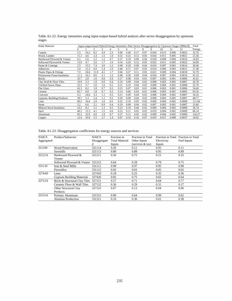
235
Table A1-22: Energy intensities using input-output-based hybrid analysis after sector disaggregation by upstream
stages
Study Material Input-output-based Hybrid Energy Intensities After Sector Disaggregation by Upstream Stages (MBtu/$) Total
Energy 0 1 2 3 4 5 6 7 8 9 10 11 12
Carpets 5.5 10.2 8.2 4.9 2.3 0.96 0.40 0.17 0.07 0.030 0.013 0.006 0.0025 32.76
Wood, Lumber 11.1 4.6 2.4 1.5 1.0 0.52 0.25 0.12 0.05 0.024 0.011 0.005 0.0021 21.56
Hardwood Plywood & Veneer 6.5 5.6 2.2 1.2 0.7 0.37 0.18 0.09 0.04 0.018 0.008 0.004 0.0016 16.83
Softwood Plywood & Veneer 13.0 4.7 2.6 1.7 1.0 0.54 0.26 0.12 0.05 0.025 0.011 0.005 0.0022 24.09
Paints & Coatings 2.5 15.5 7.4 3.0 1.2 0.49 0.20 0.09 0.04 0.016 0.007 0.003 0.0014 30.46
Adhesives 5.0 12.3 6.0 2.4 1.0 0.40 0.17 0.07 0.03 0.014 0.006 0.003 0.0012 27.49
Plastic Pipes & Fittings 7.0 26.6 11.9 4.5 1.7 0.66 0.27 0.11 0.05 0.021 0.009 0.004 0.0018 52.79
Polystyrene Foam Insulation 11.3 16.2 8.6 3.1 1.2 0.48 0.20 0.09 0.04 0.016 0.007 0.003 0.0014 41.23
Bricks 35.7 2.8 1.6 0.8 0.4 0.17 0.08 0.03 0.01 0.007 0.003 0.001 0.0006 41.61
Clay Wall & Floor Tiles 19.9 3.3 1.9 0.9 0.4 0.19 0.09 0.04 0.02 0.008 0.003 0.002 0.0007 26.78
Vitrified Sewer Pipes 25.2 3.7 2.0 1.0 0.5 0.21 0.10 0.04 0.02 0.009 0.004 0.002 0.0008 32.76
Flat Glass 43.3 8.2 1.8 0.7 0.3 0.15 0.07 0.03 0.01 0.006 0.003 0.001 0.0006 54.60
Cement 83.7 6.8 1.8 0.7 0.3 0.14 0.06 0.03 0.01 0.006 0.003 0.001 0.0005 93.56
Concrete 4.3 24.6 3.3 1.1 0.5 0.21 0.09 0.04 0.02 0.008 0.004 0.002 0.0007 34.16
Gypsum, Building Products 39.1 5.3 2.4 1.1 0.5 0.20 0.09 0.04 0.02 0.008 0.003 0.002 0.0007 48.77
Lime 90.2 16.6 2.9 1.0 0.5 0.22 0.10 0.05 0.02 0.009 0.004 0.002 0.0009 111.60
Stone 5.2 6.6 2.1 0.9 0.4 0.19 0.08 0.04 0.02 0.007 0.003 0.001 0.0007 15.60
Mineral Wool Insulation 23.2 8.2 3.1 1.3 0.5 0.23 0.10 0.04 0.02 0.009 0.004 0.002 0.0008 36.74
Steel 40.2 13.3 4.1 1.5 0.6 0.25 0.11 0.05 0.02 0.010 0.004 0.002 0.0009 60.14
Aluminum 95.2 22.0 6.0 1.9 0.7 0.27 0.11 0.05 0.02 0.009 0.004 0.002 0.0009 126.27
Copper 12.4 10.8 5.5 2.7 1.4 0.67 0.32 0.16 0.07 0.035 0.017 0.008 0.0037 34.02
Table A1-23: Disaggregation coefficients for energy sources and services
NAICS Aggregated
Product/Subsector NAICS Disaggregate
d
Fraction in Total Material
Inputs
Fraction in Total Other Inputs
(services & tax)
Fraction in Total Electricity
Inputs
Fraction in Total Fuel Inputs
321100 Wood Preservation 321114 0.20 0.12 0.05 0.11
Sawmills 321113 0.80 0.88 0.95 0.89
32121A Hardwood Plywood &
Veneer
321211 0.36 0.72 0.21 0.25
Softwood Plywood & Veneer 321212 0.64 0.28 0.79 0.75
331110 Iron & Steel Mills 331111 0.98 0.97 0.95 0.98
Ferroalloy 331112 0.02 0.03 0.05 0.02
3274A0 Lime 327410 0.18 0.25 0.35 0.36
Gypsum Building Materials 327420 0.82 0.75 0.65 0.64
32712A Brick & Structural Clay Tiles 327121 0.57 0.71 0.64 0.77
Ceramic Floor & Wall Tiles 327122 0.36 0.29 0.31 0.17
Other Structural Clay Products
327123 0.07 0.13 0.04 0.06
33131A Primary Aluminum 331312 0.90 0.64 0.99 0.62
Alumina Production 331311 0.10 0.36 0.01 0.38
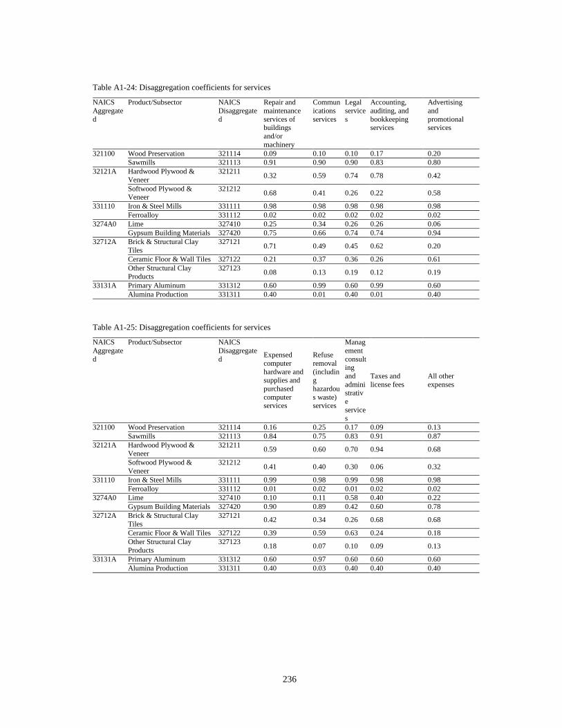
236
Table A1-24: Disaggregation coefficients for services
NAICS
Aggregate
d
Product/Subsector NAICS
Disaggregate
d
Repair and
maintenance
services of buildings
and/or
machinery
Commun
ications
services
Legal
service
s
Accounting,
auditing, and
bookkeeping services
Advertising
and
promotional services
321100 Wood Preservation 321114 0.09 0.10 0.10 0.17 0.20
Sawmills 321113 0.91 0.90 0.90 0.83 0.80
32121A Hardwood Plywood &
Veneer
321211 0.32 0.59 0.74 0.78 0.42
Softwood Plywood & Veneer
321212 0.68 0.41 0.26 0.22 0.58
331110 Iron & Steel Mills 331111 0.98 0.98 0.98 0.98 0.98
Ferroalloy 331112 0.02 0.02 0.02 0.02 0.02
3274A0 Lime 327410 0.25 0.34 0.26 0.26 0.06
Gypsum Building Materials 327420 0.75 0.66 0.74 0.74 0.94
32712A Brick & Structural Clay
Tiles
327121 0.71 0.49 0.45 0.62 0.20
Ceramic Floor & Wall Tiles 327122 0.21 0.37 0.36 0.26 0.61
Other Structural Clay Products
327123 0.08 0.13 0.19 0.12 0.19
33131A Primary Aluminum 331312 0.60 0.99 0.60 0.99 0.60
Alumina Production 331311 0.40 0.01 0.40 0.01 0.40
Table A1-25: Disaggregation coefficients for services
NAICS
Aggregate
d
Product/Subsector NAICS
Disaggregate
d Expensed
computer
hardware and supplies and
purchased
computer services
Refuse
removal
(including
hazardou
s waste) services
Manag
ement
consulting
and
administrativ
e
services
Taxes and
license fees
All other
expenses
321100 Wood Preservation 321114 0.16 0.25 0.17 0.09 0.13
Sawmills 321113 0.84 0.75 0.83 0.91 0.87
32121A Hardwood Plywood & Veneer
321211 0.59 0.60 0.70 0.94 0.68
Softwood Plywood &
Veneer
321212 0.41 0.40 0.30 0.06 0.32
331110 Iron & Steel Mills 331111 0.99 0.98 0.99 0.98 0.98
Ferroalloy 331112 0.01 0.02 0.01 0.02 0.02
3274A0 Lime 327410 0.10 0.11 0.58 0.40 0.22
Gypsum Building Materials 327420 0.90 0.89 0.42 0.60 0.78
32712A Brick & Structural Clay
Tiles
327121 0.42 0.34 0.26 0.68 0.68
Ceramic Floor & Wall Tiles 327122 0.39 0.59 0.63 0.24 0.18
Other Structural Clay
Products
327123 0.18 0.07 0.10 0.09 0.13
33131A Primary Aluminum 331312 0.60 0.97 0.60 0.60 0.60
Alumina Production 331311 0.40 0.03 0.40 0.40 0.40
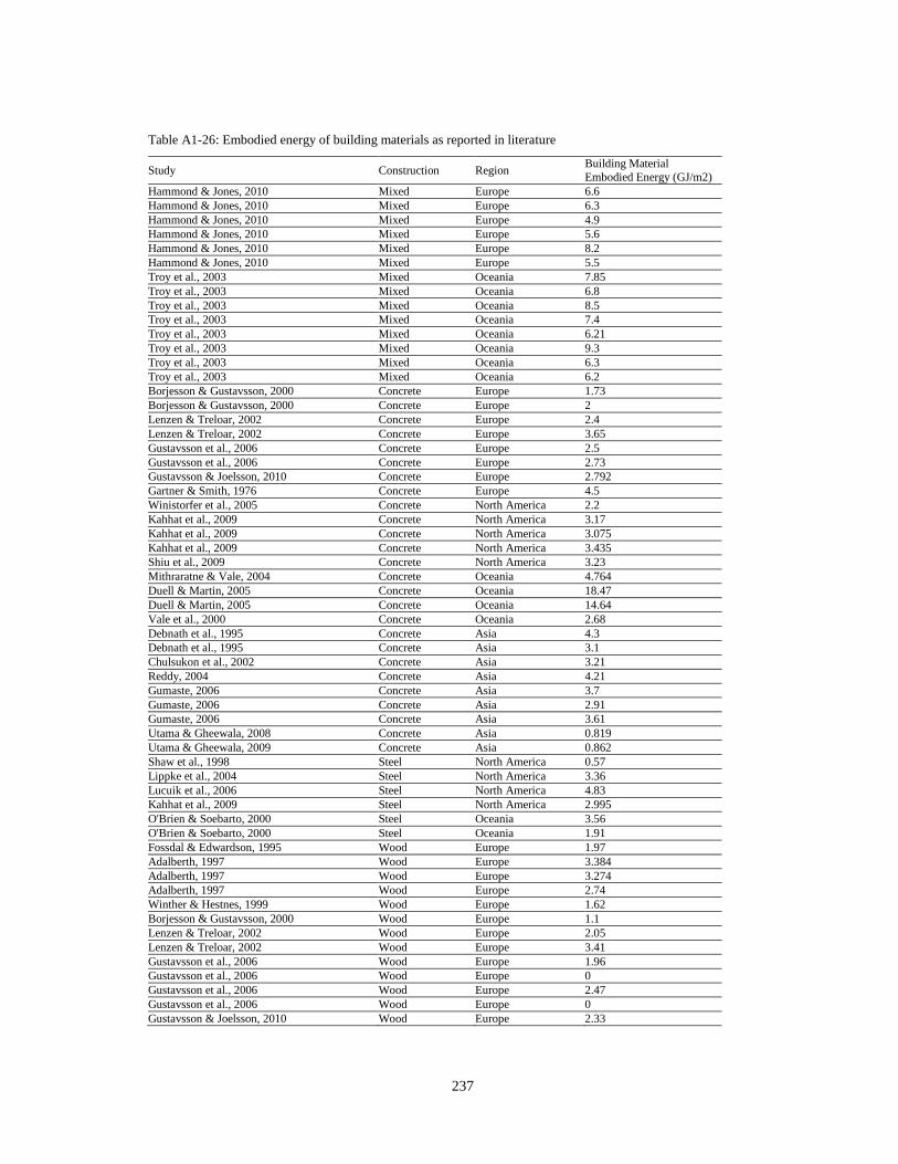
237
Table A1-26: Embodied energy of building materials as reported in literature
Study Construction Region Building Material
Embodied Energy (GJ/m2)
Hammond & Jones, 2010 Mixed Europe 6.6
Hammond & Jones, 2010 Mixed Europe 6.3
Hammond & Jones, 2010 Mixed Europe 4.9
Hammond & Jones, 2010 Mixed Europe 5.6
Hammond & Jones, 2010 Mixed Europe 8.2
Hammond & Jones, 2010 Mixed Europe 5.5
Troy et al., 2003 Mixed Oceania 7.85
Troy et al., 2003 Mixed Oceania 6.8
Troy et al., 2003 Mixed Oceania 8.5
Troy et al., 2003 Mixed Oceania 7.4
Troy et al., 2003 Mixed Oceania 6.21
Troy et al., 2003 Mixed Oceania 9.3
Troy et al., 2003 Mixed Oceania 6.3
Troy et al., 2003 Mixed Oceania 6.2
Borjesson & Gustavsson, 2000 Concrete Europe 1.73
Borjesson & Gustavsson, 2000 Concrete Europe 2
Lenzen & Treloar, 2002 Concrete Europe 2.4
Lenzen & Treloar, 2002 Concrete Europe 3.65
Gustavsson et al., 2006 Concrete Europe 2.5
Gustavsson et al., 2006 Concrete Europe 2.73
Gustavsson & Joelsson, 2010 Concrete Europe 2.792
Gartner & Smith, 1976 Concrete Europe 4.5
Winistorfer et al., 2005 Concrete North America 2.2
Kahhat et al., 2009 Concrete North America 3.17
Kahhat et al., 2009 Concrete North America 3.075
Kahhat et al., 2009 Concrete North America 3.435
Shiu et al., 2009 Concrete North America 3.23
Mithraratne & Vale, 2004 Concrete Oceania 4.764
Duell & Martin, 2005 Concrete Oceania 18.47
Duell & Martin, 2005 Concrete Oceania 14.64
Vale et al., 2000 Concrete Oceania 2.68
Debnath et al., 1995 Concrete Asia 4.3
Debnath et al., 1995 Concrete Asia 3.1
Chulsukon et al., 2002 Concrete Asia 3.21
Reddy, 2004 Concrete Asia 4.21
Gumaste, 2006 Concrete Asia 3.7
Gumaste, 2006 Concrete Asia 2.91
Gumaste, 2006 Concrete Asia 3.61
Utama & Gheewala, 2008 Concrete Asia 0.819
Utama & Gheewala, 2009 Concrete Asia 0.862
Shaw et al., 1998 Steel North America 0.57
Lippke et al., 2004 Steel North America 3.36
Lucuik et al., 2006 Steel North America 4.83
Kahhat et al., 2009 Steel North America 2.995
O'Brien & Soebarto, 2000 Steel Oceania 3.56
O'Brien & Soebarto, 2000 Steel Oceania 1.91
Fossdal & Edwardson, 1995 Wood Europe 1.97
Adalberth, 1997 Wood Europe 3.384
Adalberth, 1997 Wood Europe 3.274
Adalberth, 1997 Wood Europe 2.74
Winther & Hestnes, 1999 Wood Europe 1.62
Borjesson & Gustavsson, 2000 Wood Europe 1.1
Lenzen & Treloar, 2002 Wood Europe 2.05
Lenzen & Treloar, 2002 Wood Europe 3.41
Gustavsson et al., 2006 Wood Europe 1.96
Gustavsson et al., 2006 Wood Europe 0
Gustavsson et al., 2006 Wood Europe 2.47
Gustavsson et al., 2006 Wood Europe 0
Gustavsson & Joelsson, 2010 Wood Europe 2.33
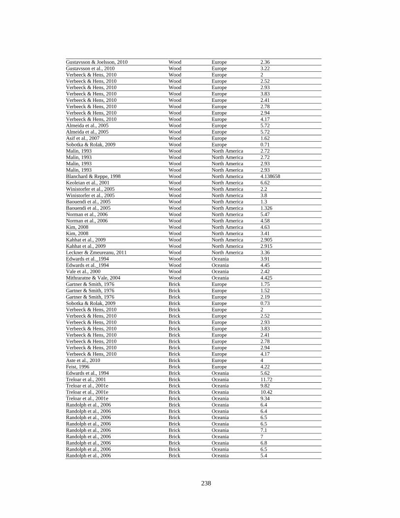
238
Gustavsson & Joelsson, 2010 Wood Europe 2.36
Gustavsson et al., 2010 Wood Europe 3.22
Verbeeck & Hens, 2010 Wood Europe 2
Verbeeck & Hens, 2010 Wood Europe 2.52
Verbeeck & Hens, 2010 Wood Europe 2.93
Verbeeck & Hens, 2010 Wood Europe 3.83
Verbeeck & Hens, 2010 Wood Europe 2.41
Verbeeck & Hens, 2010 Wood Europe 2.78
Verbeeck & Hens, 2010 Wood Europe 2.94
Verbeeck & Hens, 2010 Wood Europe 4.17
Almeida et al., 2005 Wood Europe 5.72
Almeida et al., 2005 Wood Europe 5.72
Asif et al., 2007 Wood Europe 1.62
Sobotka & Rolak, 2009 Wood Europe 0.71
Malin, 1993 Wood North America 2.72
Malin, 1993 Wood North America 2.72
Malin, 1993 Wood North America 2.93
Malin, 1993 Wood North America 2.93
Blanchard & Reppe, 1998 Wood North America 4.138658
Keoleian et al., 2001 Wood North America 6.62
Winistorfer et al., 2005 Wood North America 2.2
Winistorfer et al., 2005 Wood North America 3.8
Baouendi et al., 2005 Wood North America 1.3
Baouendi et al., 2005 Wood North America 1.326
Norman et al., 2006 Wood North America 5.47
Norman et al., 2006 Wood North America 4.58
Kim, 2008 Wood North America 4.63
Kim, 2008 Wood North America 3.41
Kahhat et al., 2009 Wood North America 2.905
Kahhat et al., 2009 Wood North America 2.915
Leckner & Zmeureanu, 2011 Wood North America 3.36
Edwards et al._1994 Wood Oceania 3.91
Edwards et al._1994 Wood Oceania 4.45
Vale et al., 2000 Wood Oceania 2.42
Mithraratne & Vale, 2004 Wood Oceania 4.425
Gartner & Smith, 1976 Brick Europe 1.75
Gartner & Smith, 1976 Brick Europe 1.52
Gartner & Smith, 1976 Brick Europe 2.19
Sobotka & Rolak, 2009 Brick Europe 0.73
Verbeeck & Hens, 2010 Brick Europe 2
Verbeeck & Hens, 2010 Brick Europe 2.52
Verbeeck & Hens, 2010 Brick Europe 2.93
Verbeeck & Hens, 2010 Brick Europe 3.83
Verbeeck & Hens, 2010 Brick Europe 2.41
Verbeeck & Hens, 2010 Brick Europe 2.78
Verbeeck & Hens, 2010 Brick Europe 2.94
Verbeeck & Hens, 2010 Brick Europe 4.17
Aste et al., 2010 Brick Europe 4
Feist, 1996 Brick Europe 4.22
Edwards et al., 1994 Brick Oceania 5.62
Treloar et al., 2001 Brick Oceania 11.72
Treloar et al., 2001e Brick Oceania 9.82
Treloar et al., 2001e Brick Oceania 10.42
Treloar et al., 2001e Brick Oceania 9.34
Randolph et al., 2006 Brick Oceania 6.4
Randolph et al., 2006 Brick Oceania 6.4
Randolph et al., 2006 Brick Oceania 6.5
Randolph et al., 2006 Brick Oceania 6.5
Randolph et al., 2006 Brick Oceania 7.1
Randolph et al., 2006 Brick Oceania 7
Randolph et al., 2006 Brick Oceania 6.8
Randolph et al., 2006 Brick Oceania 6.5
Randolph et al., 2006 Brick Oceania 5.4

239
Randolph et al., 2006 Brick Oceania 8.3
Randolph et al., 2006 Brick Oceania 7.9
Randolph et al., 2006 Brick Oceania 6.7
Debnath et al., 1995 Brick Asia 5
Debnath et al., 1995 Brick Asia 4.2
Debnath et al., 1995 Brick Asia 4.1
Debnath et al., 1995 Brick Asia 3.7
Chulsukon et al., 2002 Brick Asia 3.21
Reddy, 2004 Brick Asia 4.21
Reddy, 2004 Brick Asia 2.92
Reddy, 2004 Brick Asia 1.61
Jeyasingh & Sam, 2004 Brick Asia 6.44
Gumaste, 2006 Brick Asia 3.67
Utama & Gheewala, 2008 Brick Asia 0.838
Utama & Gheewala, 2009 Brick Asia 0.862
Utama & Gheewala, 2009 Brick Asia 0.926
Huberman & Pearlmutter, 2004 Brick Asia 0.77
Huberman & Pearlmutter, 2004 Brick Asia 1.06
Huberman & Pearlmutter, 2004 Brick Asia 3.52
Huberman & Pearlmutter, 2004 Brick Asia 3.8
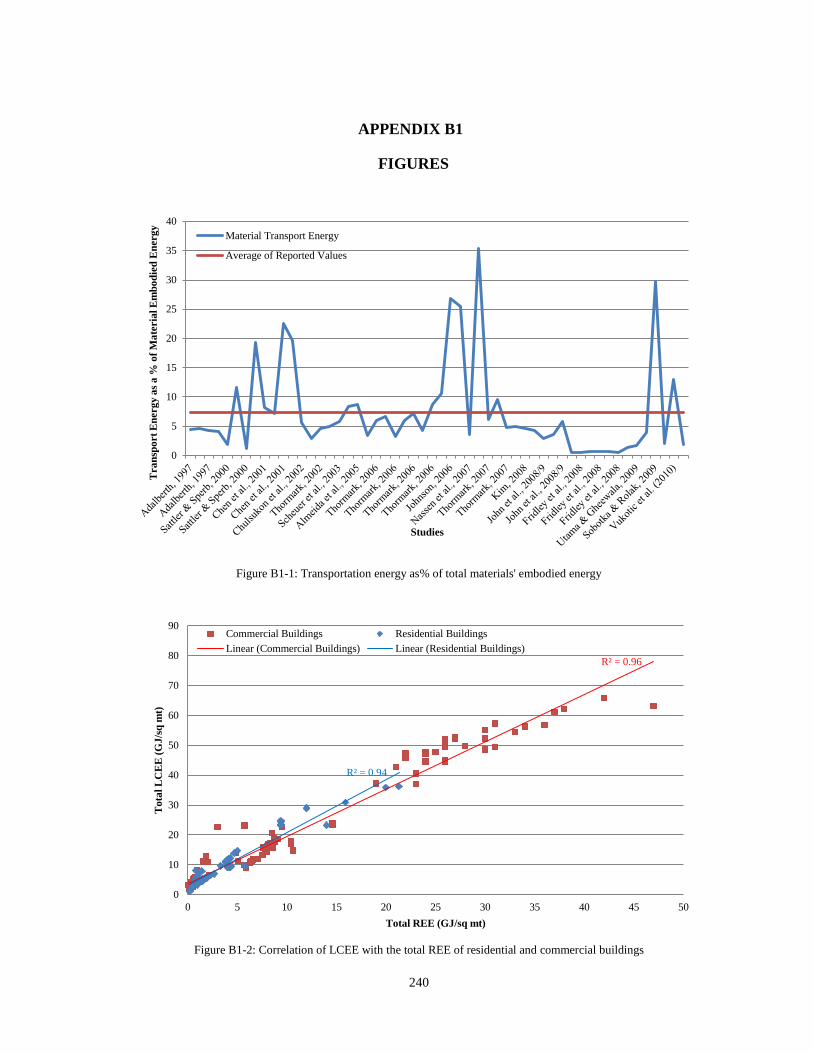
240
APPENDIX B1
FIGURES
Figure B1-1: Transportation energy as% of total materials' embodied energy
Figure B1-2: Correlation of LCEE with the total REE of residential and commercial buildings
0
5
10
15
20
25
30
35
40
Tra
nsp
ort
En
erg
y a
s a
% o
f M
ate
ria
l E
mb
od
ied
En
erg
y
Studies
Material Transport Energy
Average of Reported Values
R² = 0.96
R² = 0.94
0
10
20
30
40
50
60
70
80
90
0 5 10 15 20 25 30 35 40 45 50
To
tal
LC
EE
(G
J/s
q m
t)
Total REE (GJ/sq mt)
Commercial Buildings Residential Buildings
Linear (Commercial Buildings) Linear (Residential Buildings)
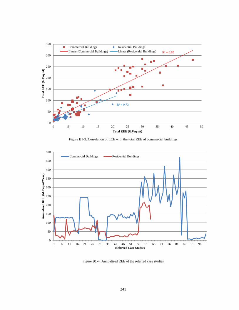
241
Figure B1-3: Correlation of LCE with the total REE of commercial buildings
Figure B1-4: Annualized REE of the referred case studies
R² = 0.83
R² = 0.73
0
50
100
150
200
250
300
350
0 5 10 15 20 25 30 35 40 45 50
To
tal
LC
E (
GJ
/sq
mt)
Total REE (GJ/sq mt)
Commercial Buildings Residential Buildings
Linear (Commercial Buildings) Linear (Residential Buildings)
0
50
100
150
200
250
300
350
400
450
500
1 6 11 16 21 26 31 36 41 46 51 56 61 66 71 76 81 86 91 96
An
nu
ali
zed
RE
E (
MJ
/sq
mt/
Yea
r)
Referred Case Studies
Commercial Buildings Residential Buildings
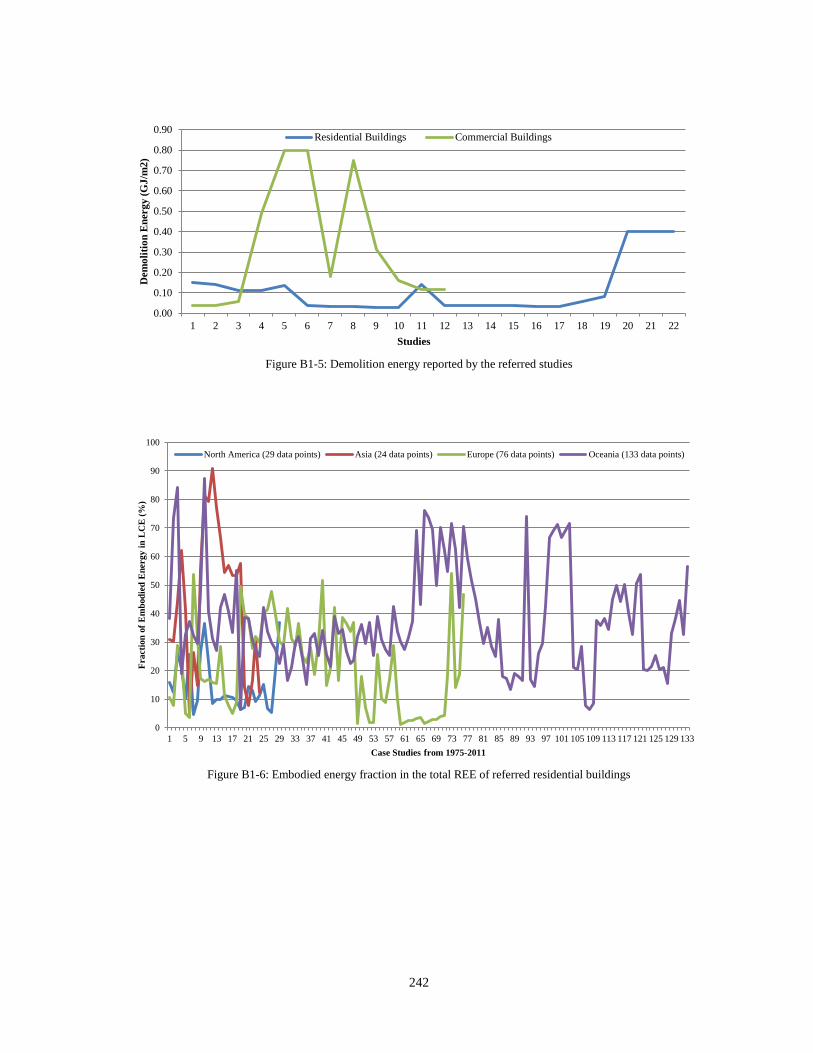
242
Figure B1-5: Demolition energy reported by the referred studies
Figure B1-6: Embodied energy fraction in the total REE of referred residential buildings
0.00
0.10
0.20
0.30
0.40
0.50
0.60
0.70
0.80
0.90
1 2 3 4 5 6 7 8 9 10 11 12 13 14 15 16 17 18 19 20 21 22
Dem
oli
tio
n E
nerg
y (
GJ
/m2
)
Studies
Residential Buildings Commercial Buildings
0
10
20
30
40
50
60
70
80
90
100
1 5 9 13 17 21 25 29 33 37 41 45 49 53 57 61 65 69 73 77 81 85 89 93 97 101 105 109 113 117 121 125 129 133
Fra
cti
on
of
Em
bod
ied
En
erg
y i
n L
CE
(%
)
Case Studies from 1975-2011
North America (29 data points) Asia (24 data points) Europe (76 data points) Oceania (133 data points)

243
Figure B1-7: Embodied energy fraction in the total REE of referred commercial buildings
0
10
20
30
40
50
60
70
1 4 7 10 13 16 19 22 25 28 31 34 37 40 43 46 49 52 55 58 61 64
Fracti
on
of
Em
bod
ied
En
ergy i
n L
CE
(%
)
Case Studies from 1993-2010
North America (36 data points) Asia (14 data points) Europe (24 data points) Oceania (64 data points)
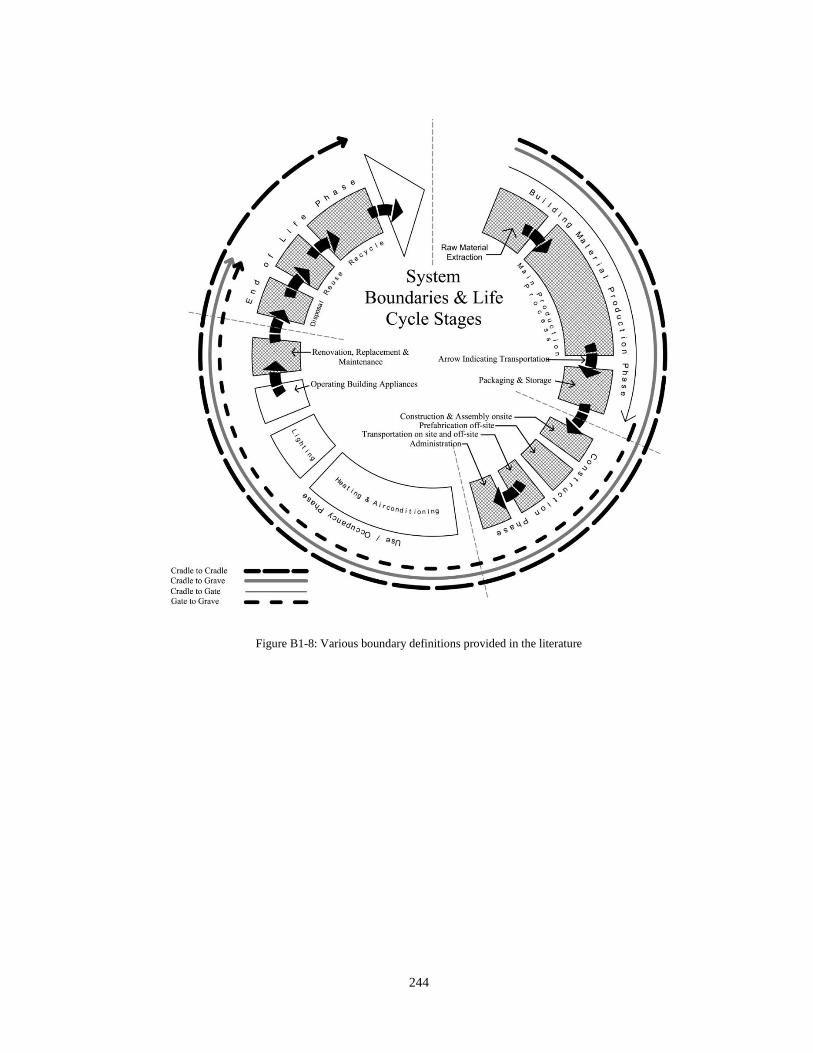
244
Figure B1-8: Various boundary definitions provided in the literature
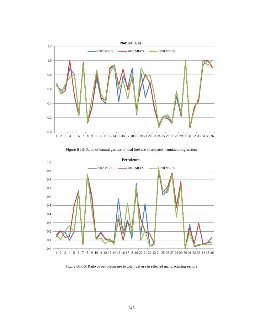
245
Figure B1-9: Ratio of natural gas use to total fuel use in selected manufacturing sectors
Figure B1-10: Ratio of petroleum use to total fuel use in selected manufacturing sectors
0.0
0.2
0.4
0.6
0.8
1.0
1.2
1 2 3 4 5 6 7 8 9 10 11 12 13 14 15 16 17 18 19 20 21 22 23 24 25 26 27 28 29 30 31 32 33 34 35 36
Natural Gas
2002 MECS 2006 MECS 1998 MECS
0.0
0.1
0.2
0.3
0.4
0.5
0.6
0.7
0.8
0.9
1.0
1 2 3 4 5 6 7 8 9 10 11 12 13 14 15 16 17 18 19 20 21 22 23 24 25 26 27 28 29 30 31 32 33 34 35 36
Petroleum
2002 MECS 2006 MECS 1998 MECS
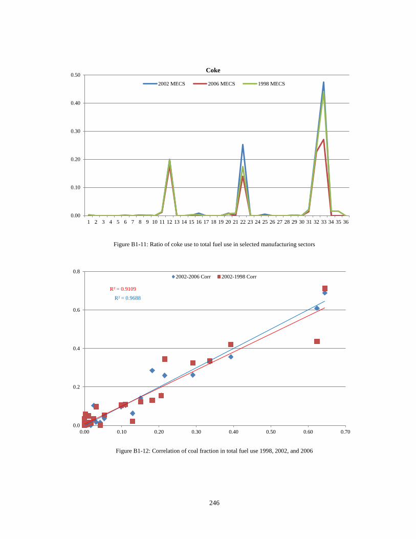
246
Figure B1-11: Ratio of coke use to total fuel use in selected manufacturing sectors
Figure B1-12: Correlation of coal fraction in total fuel use 1998, 2002, and 2006
0.00
0.10
0.20
0.30
0.40
0.50
1 2 3 4 5 6 7 8 9 10 11 12 13 14 15 16 17 18 19 20 21 22 23 24 25 26 27 28 29 30 31 32 33 34 35 36
Coke
2002 MECS 2006 MECS 1998 MECS
R² = 0.9688
R² = 0.9109
0.0
0.2
0.4
0.6
0.8
0.00 0.10 0.20 0.30 0.40 0.50 0.60 0.70
2002-2006 Corr 2002-1998 Corr
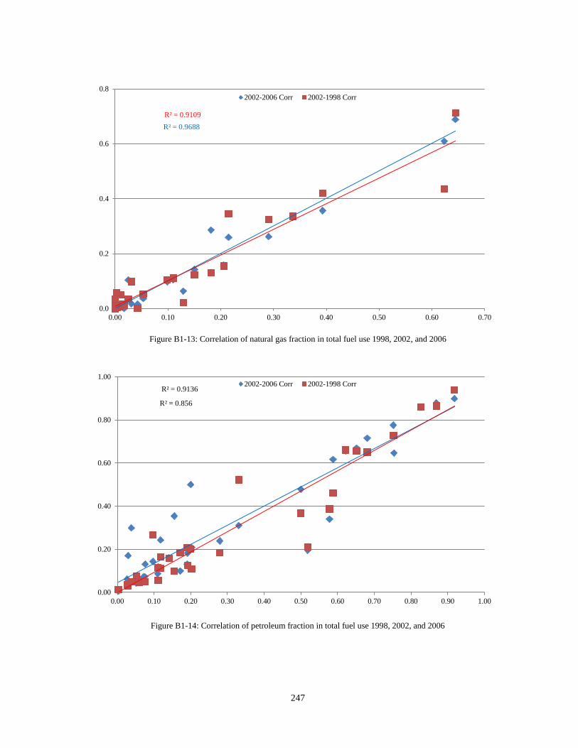
247
Figure B1-13: Correlation of natural gas fraction in total fuel use 1998, 2002, and 2006
Figure B1-14: Correlation of petroleum fraction in total fuel use 1998, 2002, and 2006
R² = 0.9688
R² = 0.9109
0.0
0.2
0.4
0.6
0.8
0.00 0.10 0.20 0.30 0.40 0.50 0.60 0.70
2002-2006 Corr 2002-1998 Corr
R² = 0.856
R² = 0.9136
0.00
0.20
0.40
0.60
0.80
1.00
0.00 0.10 0.20 0.30 0.40 0.50 0.60 0.70 0.80 0.90 1.00
2002-2006 Corr 2002-1998 Corr
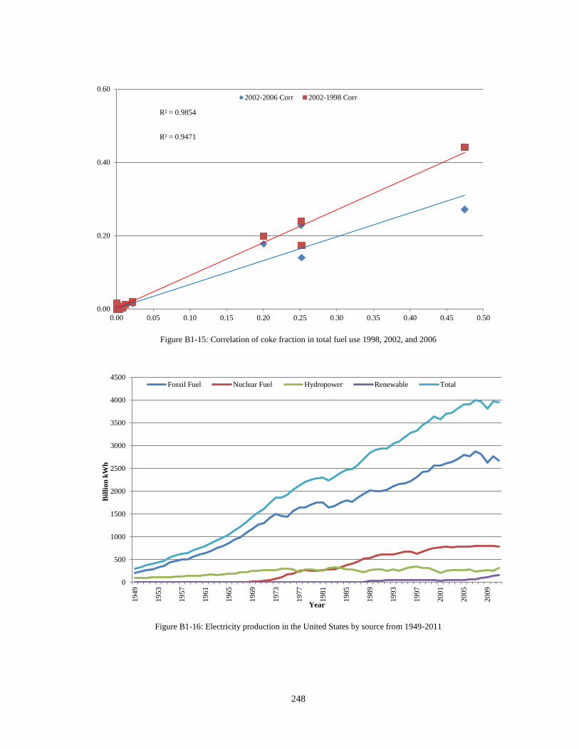
248
Figure B1-15: Correlation of coke fraction in total fuel use 1998, 2002, and 2006
Figure B1-16: Electricity production in the United States by source from 1949-2011
R² = 0.9471
R² = 0.9854
0.00
0.20
0.40
0.60
0.00 0.05 0.10 0.15 0.20 0.25 0.30 0.35 0.40 0.45 0.50
2002-2006 Corr 2002-1998 Corr
0
500
1000
1500
2000
2500
3000
3500
4000
4500
19
49
19
53
19
57
19
61
19
65
19
69
19
73
19
77
19
81
19
85
19
89
19
93
19
97
20
01
20
05
20
09
Bil
lio
n k
Wh
Year
Fossil Fuel Nuclear Fuel Hydropower Renewable Total
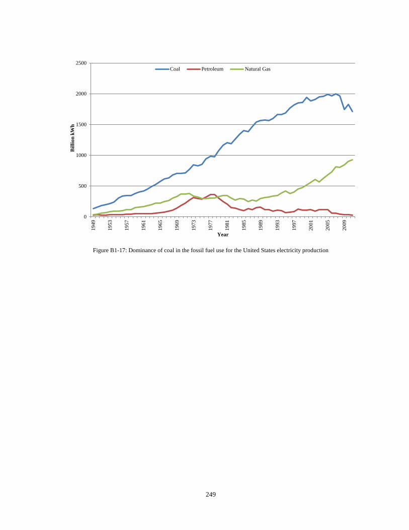
249
Figure B1-17: Dominance of coal in the fossil fuel use for the United States electricity production
0
500
1000
1500
2000
2500
19
49
19
53
19
57
19
61
19
65
19
69
19
73
19
77
19
81
19
85
19
89
19
93
19
97
20
01
20
05
20
09
Bil
lio
n k
Wh
Year
Coal Petroleum Natural Gas
250
APPENDIX C1
ARTICLES RESULTING FROM THE RESEARCH
Journal Papers
Dixit, M.K., Culp, C.H. Fernández-Solís, J.L. (2013). “System boundary for embodied energy in
buildings: A conceptual model for definition.” Renewable and Sustainable Energy Reviews, 21,
153-164.
Dixit, M.K., Fernández-Solís, J.L., Lavy, S., and Culp, C.H. (2012). “Need for an embodied
energy measurement protocol for buildings: A review paper.” Renewable and Sustainable Energy
Reviews, 16 (6), 3730-3743.
Dixit, M.K., Culp, C.H., Lavy, S., and Fernández-Solís, J.L. (2012). “Recurrent Embodied
Energy in Life Cycle of Built Facilities.” Facilities, accepted for publication.
Dixit, M.K., Fernández-Solís, J.L., Lavy, S., and Culp, C.H. (2010). “Identification of parameters
for embodied energy measurement: A literature review.” Energy and Buildings, 42 (8), 1238-
1247.
Conference Proceedings
Dixit, M.K., and Yan, W. (2012). “BIM-based BiPV prototype for the solar insolation
calculation. In: ISG-ISARC Conference on Robotics and Automation in Construction,”
Eindhoven, June 26-29, 2012.
Dixit, M.K., Culp, C.H., Lavy, S., and Fernández-Solís, J.L., (2012). “Recurrent embodied
energy and its relationship with service life and life cycle energy: a review paper.” In: Joint CIB
W070, W092 and TG72 International Conference, Cape Town, January 22-25, 2012.
Dixit, M.K., Fernández-Solís, J.L., Lavy, S., and Culp, C.H. (2010). “State of Standardization in
Embodied Energy Computation: The need for a Protocol.” In: Proceedings of the CIB-W70
International Conference in Facilities Management: FM in the Experience Economy, Sao Paulo,
September 13-15, 2010, pp. 571-583.
Dixit, M.K., Fernández-Solís, J.L., Lavy, S., and Culp, C.H. (2010). “Protocol for Embodied
energy Measurement Parameters.” In: Proceedings of the TG66 - Special Track 18th CIB World
Building Congress, Salford, UK, May 11-13, 2010, pp. 188-203.