emanuela giannini - imprs hd · m.sc. emanuela giannini ... a lea e rosa 5. nothing is ever really...
TRANSCRIPT
MiNDSTEp differential photometry of the gravitationally lensedquasars WFI2033-4723, HE0047-1756 and Q2237+0305
Emanuela Giannini
2016

Cover picture: The Phoenix, Marisa Milan (2014)
2
Dissertation
submitted to the
Combined Faculties of Natural Sciences and Mathematics
of the Ruperto-Carola-University of Heidelberg, Germany
for the degree of
Doctor of Natural Sciences
Put forward by
Emanuela Giannini
born in: Colleferro (RM), Italy
Oral examination: February 8th, 2017


MiNDSTEp differential photometry of the gravitationally lensedquasars WFI2033-4723, HE0047-1756 and Q2237+0305
M.Sc. Emanuela GianniniAstronomisches Rechen–Institut
Zentrum fur Astronomie der Universitat HeidelbergFakultat fur Physik und Astronomie
Referees: Prof. Dr. Joachim WambsganssDr. Sabine Reffert


A Lea e Rosa
5


Nothing is ever really lost, or can belost,No birth, identity, form–no object ofthe world.Nor life, nor force, nor any visiblething;Appearance must not foil, nor shiftedsphere confuse thy brain.Ample are time and space–ample thefields of Nature.The body, sluggish, aged, cold–theembers left from earlier fires,The light in the eye grown dim, shallduly flame again;The sun now low in the west rises formornings and for noons continual;To frozen clods ever the spring’sinvisible law returns,With grass and flowers and summerfruits and corn.
Continuities—WW
Never, never, never give up.
—W C
7

Abstract
This work focusses on studying the brightness variation of gravitationally lensedmultiply imaged quasars. The main goal is the optimization of the relative differen-tial photometry procedures, which are based on the difference image analysis (DIA)method. Moreover, it aims at isolating uncorrelated flux variations among the quasarimages, which can be explained as due to quasar microlensing events, and at the esti-mation of the time delays of the observed systems from the retrieved light curves.We present V and R photometry of the gravitationally lensed quasars WFI 2033-4723,HE 0047-1756 and Q 2237+0305. The analyzed data belong to the MiNDSTEp collab-oration and were taken with the 1.54 m Danish telescope at ESO/La Silla from 2008 to2012. The differential photometry is based on the already published method by Alard &Lupton as implemented in the HOTPAnTS package, and additionally uses the GALFITpackage for obtaining the quasar photometry.The quasar WFI 2033-4723 shows brightness variations of ≈ 0.5 mag in V and R dur-ing the campaign. The two lensed components of quasar HE 0047-1756 vary by ≈0.2− 0.3 mag within five years. We provide for the first time an estimate of the timedelay of component B with respect to A of ∆t = (7.6±1.8) days for this object. We alsofind evidence for a secular evolution of the magnitude difference between componentsA and B in both filters, which we explain as due to a long-duration microlensing event.We also find that both quasars WFI 2033-4723 and HE 0047-1756 become bluer whenbrighter, which is consistent with previous studies. The quasar Q 2237+0305 shows im-pressive uncorrelated variations of the four components in both the V and R bands, withbrightness variations between ≈ 0.2 and ≈ 1.3 mag. In particular, component D showsflux variations of ≈ 1.3 mag in the V band and ≈ 0.8 mag in the R band during the 5-yearmonitoring campaign, along a caustic-crossing feature of the light curve. We also findthat the color of this component becomes redder by ≈ 0.6 mag while it becomes fainter.Image C becomes brighter by ≈ 0.7 mag between the last two monitoring seasons andthis again suggests a high-magnification microlensing event.
Zusammenfassung
Diese Arbeit konzentriert sich auf die Studie der Helligkeitsveranderung von mehrfachabgebildeten gravitationsgelinsten Quasaren. Das Hauptziel ist die Optimierung der rel-ativen differentiellen Photometrie-Verfahren, die auf Methoden der Differenz-Bildanalyse(DIA) basieren. Daruber hinaus strebt sie die Isolation unkorrelierter Fluss-Variationunter den Quasar-Bildern an, die durch Quasar-Mikrolinsenereignisse erklart werdenkonnen, und beabsichtigt die Schatzung von Zeitverzogerungen der beobachteten Sys-teme von den gewonnenen Lichtkurven. Wir prasentieren V- und R-Photometrie der
i
gravitationsgelinsten Quasare WFI 2033-4723, HE 0047-1756 und Q 2237+0305. Dieanalysierten Daten gehoren zum MiNDSTEp-Kollaboratorium und wurden mit dem1,54 m großen Danischen Teleskop in ESO/La Silla zwischen 2008 und 2012 aufgenom-men. Die differentielle Photometrie basiert auf der bereits veroffentlichten Alard- undLupton-Methode, wie sie im HOTPAnTS-Paket implementiert wurde, und verwendetzusatzlich das GALFIT-Paket, um die Quasar-Photometrie zu bestimmen. Der QuasarWFI 2033-4723 zeigt wahrend der Kampagne Helligkeitsveranderungen in einer Großevon ≈ 0,5 mag in V und R. Die beiden gelinsten Komponenten des Quasars HE 0047-1756 variieren zwischen ≈ 0,2−0,3 mag innerhalb von funf Jahren. Fur dieses Objektbieten wir erstmals eine Schatzung der Zeitverzogerung der Komponente B im Bezugauf A von ∆t = (7,6±1,8) Tagen an. Weiterhin finden wir in beiden Filtern einen Hin-weis fur eine sakulare Evolution des Helligkeitsunterschiedes zwischen den Komponen-ten A und B, die wir durch ein lang anhaltendes Mikrolinsenereignis erklaren konnen.Wir finden außerdem heraus, dass beide Quasare, WFI 2033-4723 und HE 0047-1756,blauer werden mit Zunahme der Helligkeit, welches konsistent mit vorherigen Stu-dien ist. Der Quasar Q 2237+0305 zeigt beeindruckende unkorrelierte Variationen inseinen vier Komponenten mit Helligkeitsveranderungen zwischen ≈ 0,2 und ≈ 1,3 magsowohl im V- als auch im R-Band. Insbesondere Komponente D zeigt Fluss-Variationeninnerhalb der funfmonatigen Beobachtungskampange von ≈ 1,3 mag im V-Band und≈ 0,8 mag im R-Band in einem kaustikahnlichen Merkmal der Lichtkurve. Wir findenaußerdem heraus, dass die Farbe dieser Komponente um ≈ 0,6 mag roter wird. Bild Cwird zwischen zwei Beobachtungssaisons um ≈ 0,7 mag heller und dies deutet ebenfallsauf ein Mikrolinsenereignis großer Verstarkung hin.
ii

Contents
Abstract i
Table of contents iii
1 Motivation 1
2 Introduction to AGNs and Quasar Microlensing 32.1 ACTIVE GALACTIC NUCLEI . . . . . . . . . . . . . . . . . . . . . 3
2.1.1 The AGN class . . . . . . . . . . . . . . . . . . . . . . . . . . 32.1.2 Black hole formation and accretion . . . . . . . . . . . . . . . 72.1.3 Zooming-in on Quasars . . . . . . . . . . . . . . . . . . . . . . 9
2.2 GRAVITATIONAL LENSING . . . . . . . . . . . . . . . . . . . . . . 92.2.1 Basic theory of gravitational lensing . . . . . . . . . . . . . . . 10
2.3 The special case of Quasar Microlensing . . . . . . . . . . . . . . . . . 16
3 Overview of the quasars studied in this work 213.1 WFI J2033-4723 . . . . . . . . . . . . . . . . . . . . . . . . . . . . . 213.2 HE 0047-1756 . . . . . . . . . . . . . . . . . . . . . . . . . . . . . . . 213.3 Q 2237+0305: Huchra’s lens . . . . . . . . . . . . . . . . . . . . . . . 24
4 The MiNDSTEp collaboration and data acquisition 294.1 MiNDSTEp: Objectives and first results . . . . . . . . . . . . . . . . . 294.2 Data acquisition . . . . . . . . . . . . . . . . . . . . . . . . . . . . . . 32
5 Data Reduction 375.1 Data storage . . . . . . . . . . . . . . . . . . . . . . . . . . . . . . . . 375.2 Flat Fielding and bias correction . . . . . . . . . . . . . . . . . . . . . 375.3 Image alignment . . . . . . . . . . . . . . . . . . . . . . . . . . . . . 38
6 Theory and Practice of Differential Image Analysis 436.1 Differential Image Analysis applied to lensed quasars: an overview . . . 436.2 Full theory of the Alard&Lupton image subtraction method with con-
stant and space-varying convolution kernels . . . . . . . . . . . . . . . 446.3 Image subtraction in practice . . . . . . . . . . . . . . . . . . . . . . . 46
6.3.1 HOTPAnTS modus operandi . . . . . . . . . . . . . . . . . . . 496.3.2 HOTPAnTS implementation . . . . . . . . . . . . . . . . . . . 49
6.4 Photometry . . . . . . . . . . . . . . . . . . . . . . . . . . . . . . . . 516.4.1 Systematics with using GALFIT . . . . . . . . . . . . . . . . . 54
iii

Contents
7 WFI 2033-4723 577.1 Light curves of the quasar WFI 2033-4723 . . . . . . . . . . . . . . . . 57
8 HE 0047-1756 638.1 Light curves of the quasar HE 0047-1756 . . . . . . . . . . . . . . . . 638.2 Time delay for HE 0047-1756 . . . . . . . . . . . . . . . . . . . . . . 65
9 Q 2237+0305 779.1 Light curves for Q 2237+0305 . . . . . . . . . . . . . . . . . . . . . . 779.2 Q 2237+0305 standard photometry: modeling the galaxy on the R-band
template . . . . . . . . . . . . . . . . . . . . . . . . . . . . . . . . . . 83
10 Summary and conclusions 8710.1 Summary . . . . . . . . . . . . . . . . . . . . . . . . . . . . . . . . . 8710.2 Conclusions and outlook . . . . . . . . . . . . . . . . . . . . . . . . . 89
11 Appendix A 91
List of figures 99
List of tables 105
Bibliography 107
Acknowledgements 125
List of publications 127
iv

1Motivation
Since the prediction of the gravitational lensing effect ([2], [44]), according to whichthe light rays emitted from a distant background source are bent by an intervening grav-itational field, first proposed in the early 18th century, impressive progress has beenmade in the attempt of observing this phenomenon. It has been classified in a varietyof regimes, called strong, weak and micro-lensing. This means that different kinds oflight sources and gravitational fields, which are placed at different distances from theobserver, concur on realising a plethora of gravitational lensing system configurations,which act on a multitude of angular scales. This phenomenon has often contributed toindependent measurements and confirmations of results obtained by applying traditionalprinciples and methods. For example it provides an independent method of measuringthe Hubble constant [121] and a further means of investigating the existence and natureof the dark matter (for a detailed review see [94]).Gravitational lensing magnifies or demagnifies the flux of the affected images, distortstheir original shapes, changes their center of light positions and produces multiple im-ages. Strong lensing usually involves a background galactic source and a foregroundlensing galaxy and produces multiple images of the source, which can be strongly dis-torted and elongated (arcs), and have angular separations of the order of arcseconds.Weak lensing happens when a foreground matter distribution, like a cluster of galaxies,affects the light sources behind it with a little overall effect that can be detected only bymeasuring the average distortion of a multitude of slightly distorted source shapes.Microlensing arises when the gravitational field of a Galactic star bends the light froma background Galactic star. It also happens when the compact objects in a foregroundgalaxy affect the light from the multiple images of a strongly lensed quasar. This givesrise to the quasar microlensing phenomenon. In these cases mutiple images are pro-duced on angular scales from milliarcseconds to microarcseconds. This implies that theproduction of the multiple images is undetactable. Nevertheless the overall flux varia-tion can be measured.To list only a few results obtained by considering the gravitational lensing phenomenonwe mention that the validity of the general theory of relativity has also been confirmedby the observation of multiply imaged quasars [20] and strongly distorted galactic arcs
1

Chapter 1. Motivation
[112].The measurement of the Hubble constant has been optimized in the last 25 years byobserving systems such as supernovae ([61], [70]), Cepheids [51] and strong lensingsystems [74].The existence of new exoplanets orbiting distant Galactic stars has been confirmedthrough the radial velocity method [82], the observation of transits [56] and, more re-cently, by the method of microlensing of Galactic bulge stars [16].Moreover, the nature of the extragalactic halos has also been investigated by studyingtheir gravitational effect on background sources [63].Of particular interest for this thesis is the fact that the spatial structure of multiply im-aged quasars has been studied by observing the effect of compact objects in foregroundgalaxies on their multiply imaged components [20]. The inner structure of quasars isnot otherwise easily accessible and quasar microlensing is a unique method for studyingthe physical sizes of these lensed systems. The method requires constant monitoring ofthe multiply imaged quasar in order to build their light curves. From those, the sourcesize can be estimated, according to the principle that the microlensing features of thelight curves depend on the size of the lensed source, which in turn depends on the ob-served wavelength. Enourmous effort has been made in this direction and many ground-and space-based observatories have contributed the coverage in wavelength and time formany multiply imaged quasars in the last 30 years ([114], [96]). In particular, the Op-tical Gravitational Lensing Experiment [111] – OGLE – has been monitoring severalmultiply imaged quasars since 1997 and has produced those among the longest existinglight curves. Despite the enourmous amount of data produced, this application of grav-itational lensing is currently shared and applied by a quite small community, meaningthat its great potential is not yet fully exploited.Here we present our implementation of an already published method of difference im-age analysis (DIA) and apply it to several multiply imaged quasars of great interest, forwhich we received data from 2008 to 2012, in order to build their light curves. Besidesanalyzing the obtained data, the aim is also to provide us with a method to retrieve lightcurves at a higher speed when getting new quasar monitoring data. The multiply imagedquasars analyzed in this work, WFI 2033-4723, HE 0047-1756 and Q 2237+0305, arevery interesting gravitational systems for which we have been able to prolong the al-ready existing light curves and proceed, in the case of HE 0047-1756, to the calculationof the time delay between its two images. This is the time lag between the arrival timeof the light rays emitted from the two images, as due to the different geometrical path-ways and the effect on light of the gravitational field they cross. The determination ofthe time delays from several lensing systems concur on the determination of the Hubbleconstant H0 at an increased statistical accuracy and constitutes one of the most valuablecontributes of gravitational lensing to Cosmology.
2
2Introduction to AGNs and Quasar
Microlensing
2.1 ACTIVE GALACTIC NUCLEI
2.1.1 The AGN classIn this section we present the basic theory behind the phenomenon of active galactic
nuclei (see [144] and references therein; see also [80]).Active galactic nuclei, shortly AGNs, are galaxies with a compact central region
which emits strongly over the entire electromagnetic spectrum. Many of them emitstrongly in the optical, UV and X-ray regimes. Others are powerful radio sources. Allemit high energy amounts from a tiny volume, comparable to that occupied by the Sunand its planetary system. AGNs are believed to host central super massive black holes(SMBHs) with masses in the range 106−1010 M�. Although all galaxies seem to containSMBHs ([92],[60]), those in AGNs accrete matter, whose gravitational energy, possi-bly along with the rotational energy of the SMBH, is transferred into electromagneticradiation. Moreover, part of the accreting material escapes from the accretion disk ascollimated jets and uncollimated outflows, which are called winds. The size scales ofthe AGN phenomenon span 11 orders of magnitude, from the event horizon scales ofthe SMBH (1013 cm) to the jet scales, which can be as large as a few Mpc [91].AGNs are among the most luminous sources in the universe, with luminosities of 1045−
1048 erg s−1. Their observational differences are generally believed to derive from look-ing at few types of AGNs from different angles with respect to a simmetry axis. Besides,the physical explanation of the observed variety of AGNs has also to be attributed totheir different accretion flows and environments. This means that the total luminosity[83] and the cosmic epoch of the AGN [150] play an important role as well.
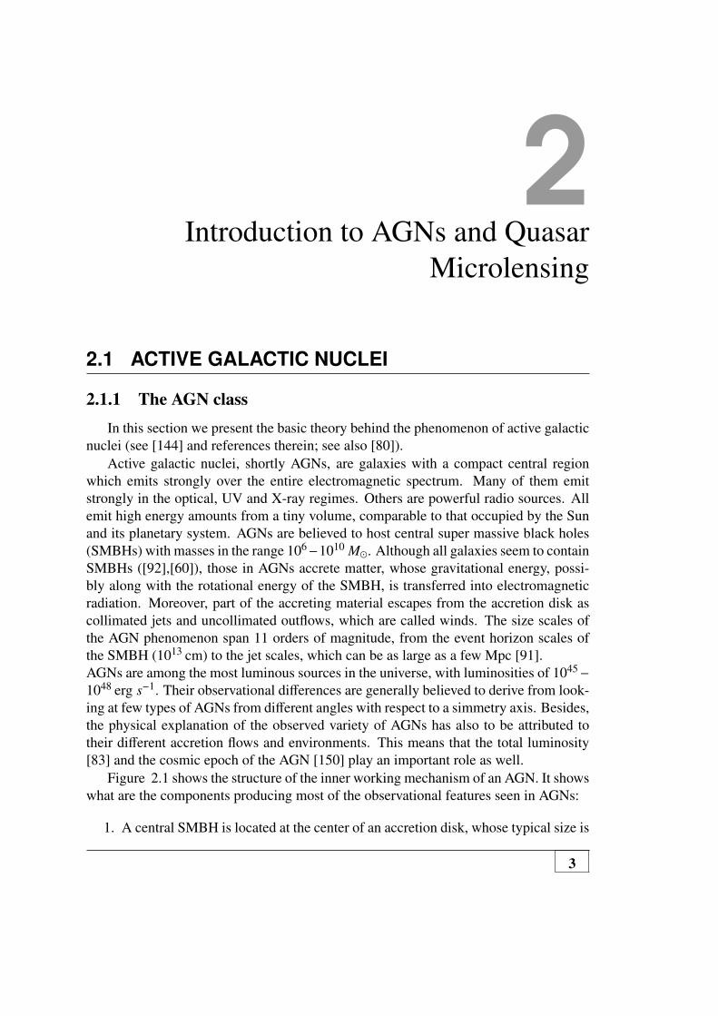
Figure 2.1 shows the structure of the inner working mechanism of an AGN. It showswhat are the components producing most of the observational features seen in AGNs:
1. A central SMBH is located at the center of an accretion disk, whose typical size is
3

Chapter 2. Introduction to AGNs and Quasar Microlensing
Figure 2.1: Sketch of the working mechanism at the basis of the AGN phenomena. Thecentral SMBH, with mass in the range 106 − 1010 M�, is surrounded by an accretiondisk, whose typical size is ∼ 1014−1015 cm. Broad emission lines are emitted from gasclouds orbiting the SMBH at a distance of ∼ 1016 −1017 cm. A dusty torus, with innerradius of ∼ 1017 cm, obscures the BLR if the AGN is observed at a large viewing anglewith respect to the simmetry axis. Clouds at much larger distances of ∼ 1018−1020 cmfrom the central engine emit narrow lines. Radio jets, in favourable conditions, arechannelled from the regions close to the SMBH (at ∼ 1015 cm) up to several 1024 cm inradio loud AGNs. The sketch is reproduced from www.oa.uj.edu.pl.
4

2.1. ACTIVE GALACTIC NUCLEI
∼ 1014−1015 cm. The accretion disk is believed to derive from gas falling into thecentral SMBH. The gas slowly flows towards the AGN center, forming a disk thatrotates around the central SMBH ([89], [138]), and whose angular momentumis transferred towards the outskirts of the disk as a result of its viscosity. Thisprocess heats the disk, which therefore radiates away its gravitational energy overa broad range of wavelengths [140]. The resulting continuum thermal emission,defined as Big Blue Bump, covers a rest frame emission range from the opticalto the soft X-ray band ([28],[78]). A fraction of the continuum emission can getcomptonized by a corona of hot material, surrounding the disk. The resultingradiation is emitted in the hard X-ray band.
2. Dense gas clouds, at ∼ 1016−1017 cm from the disk, constitute the Broad Line Re-gion (BLR), which gives rise to broad emission lines. The line widths reveal thatthe orbital speed of the emitting gas clouds is of the order of ∼ 104 kms−1. Fartherclouds, placed at a ∼ 1018−1020 cm distance, constitute the Narrow Line Region(NLR), which emits much narrower emission lines, with widths correspondingto orbital velocities below 103 kms−1. The lines from strongly ionized atoms inthe BLR vary according to the continuum variations with time lags of a few days.The low-ionized atom lines instead vary with delays of a few weeks, as one wouldexpect if they are excited at larger distances from the central nucleus. The narrowemission lines, on the other hand, do not show any significative variations, sincethey originate much farther away from the central engine. 1
3. In a radio-loud AGN, favorable conditions (i.e. strong magnetic fields) have de-termined the formation of collimated, highly relativistic radio jets, which ex-tend from the inner regions of the AGN over distances as long as ∼ 1024 cm.The jets, in the regions adjacent to the SMBH, are believed to be mostly madeup by electromagnetic radiation. At distances of ∼pc, the electromagnetic en-ergy in transferred to electrons, positrons or to the Interstellar Medium (ISM)([120],[88],[131], [14]).
Roughly 10%− 20% of AGNs are radio loud. They are classified in two types[48]: the low-power Fanaroff-Riley Class I (FRI), with radio features distributedcloser to the center, and the high-power Fanaroff-Riley Class II (FRII), with largerdistances between the jet extremities, of the order of a few Mpc.
A large number of radio-loud AGNs also shows X-ray emission from the jets
1Observations of the BLR emission lines and the disk continuum emission provide a means of esti-mating the mass of the SMBH, by making use of the reverberation mapping technique [117]. This methoduses the widths of the emission lines (from which the orbital velocities of the clouds are estimated) andthe time lags between the variability of the continuum and that of the line fluxes (hence an estimate ofthe distance between the engine and the BLR). Velocity and distance of the BLR provide the orbitalparameters necessary for the estimation of the SMBH mass.
5
Chapter 2. Introduction to AGNs and Quasar Microlensing
[62]. For the Fanaroff-Riley I, the radio to X-ray emission well matches the Syn-chrotron emission from TeV electrons in magnetic fields of < 1000 µG. On theother hand, for the Fanaroff-Riley II, the radio to X-ray spectrum is not well rep-resented by a single Synchrotron component. For these sources, the electromag-netic spectrum between the optical and the γ-ray bands becomes brighter. Thismight be due to inverse Compton scattering of Cosmic Microwave Background(CMB) photons from highly relativistic electrons ([12], [5], [176]).
AGNs jets might play a role in galactic and galaxy cluster systems, because oftheir possible contribution to the heating processes of the ISM and intraclustermedium, which would ultimately affect the star formation process [97].
4. A thick dusty torus, with an inner radius of ∼ 1017 cm, obscures the accretion diskand the BLR when the AGN is observed at an angle with respect to its simmetryaxis. It re-emits the central engine continuum in the infrared. The presence of theabove torus can explain some of the differences between different AGN classes([46], [106]). The appearance of the observed object depends on the viewingangle, whether or not the AGN has a jet emission, and the luminosity of the centralengine. If the torus is on the line of sight towards the AGN, it will conceal the BLRand only narrow lines will be observed, producing the Type-2 Seyfert galaxies(all Seyfert galaxies are in general quite modest radio sources found in spiralgalaxies) and the narrow line FRI and FRII radio galaxies (all FRI and FRII radiogalaxies are in general observed in giant elliptical galaxies, with highly polarizedsynchrotron radiation up to 1012 L�). If the torus does not obscure the BLR,the AGN will appear as Type-1 Seyfert galaxies, radio quiet quasi-stellar objects(QSOs), broad line FRI and FRII radio galaxies and quasars, quasi stellar radiosources. Although the terms quasar and QSO are today widely used as synonims– and we will only use the term quasar in the following – the word quasar wasintroduced to describe extremely luminous, high-redshift, star-like radio sources,while the term QSO was attributed later to apparently stellar sources with nointense radio counterparts. Quasars are today regarded as powerful versions ofa Seyfert galaxy, with the bolometric luminosity of transition between the twoclasses at ∼ 1011 L�. Both emit abundantly from the infrared to the X-rays, mostof them are not strong radio emitters. At small observing angles, the non-thermalcontinuum emission from the relativistic jets will prevail and the quasars willappear as radio-loud blazars, with strong variability on scales of days and stronglypolarized optical and radio emission.
5. The observation of blue-shifted broad and narrow absorption lines from the opti-cal to the X-ray wavelengths implies the existence of fast AGN outflows or winds[22]. The location at which the broad absorption line (BAL) winds are loaded isstill uncertain, whereas it is believed that the narrow absorption line (NAL) winds
6

2.1. ACTIVE GALACTIC NUCLEI
are launched at about the same distance as the NLR, of the order of ∼pc.
The emission from AGNs is in general a means of studying the objects, diffuse matterand radiation fields between us and the AGNs.
2.1.2 Black hole formation and accretionAccording to most black hole (BH) formation models, primordial black holes ap-
peared at redshift z larger than 15. There are two leading scenarios explaining howthe first black holes have appeared. The first states that the primordial BHs are thefinal product of the evolution of the first ultra metal-poor generation of stars. SuchBHs emerged at z∼ 20 with masses 100−1000 M� ([167],[103]). The other scenario at-tributes the formation of 102−105 M� BHs to direct gas collapse at z∼ 10−15 ([17],[33]).Since the typical observed SMBH mass is of 106−109 M�, most of the growth happensin AGN systems, particularly in quasars ([89], [143],[148]). Their activity is likely ig-nited by major mergers of two massive galaxies [13] and is often referred to as quasarphase. A clear correlation between the quasar phase and major mergers has been ob-served in some luminous quasars and infrared luminous star forming galaxies [128]. Onthe other hand, most AGNs are neither in mergers nor in particularly populated envi-ronments [32]. Other galaxy internal interactions might explain the moderate activity inthese AGNs, defined as secular-driven AGNs ([32], [100], [79]). Several studies ([151],[149]) show that the number of AGNs driven by secular processes is about 10 timeslarger than that of merger-driven AGNs. The latter make up for the ∼ 60% of the wholeSMBH growth at high redshifts z> 1, where mergers are gas richer and relatively morenumerous [67]. The amount of matter that the SMBH accretes during the quasar phase,which lasts ∼ 108 years ([93], [139], [34]), is of about 108 M�.
7

Chapter 2. Introduction to AGNs and Quasar Microlensing
Figu
re2.
2:A
mea
nqu
asar
spec
trum
obta
ined
byav
erag
ing
spec
tra
ofm
ore
than
700
quas
ars
from
the
Lar
geB
righ
tQua
sar
Surv
ey[5
0].T
hem
ain
emis
sion
lines
are
indi
cate
d.C
ourt
esy
ofP.
J.Fr
anci
san
dC
.B.F
oltz
.Ada
pted
from
[1].
8

2.2. GRAVITATIONAL LENSING
2.1.3 Zooming-in on Quasars
Quasars are the most luminous and distant objects among the AGNs. They wereidentified as stellar-appearing, highly redshifted sources of radio and optical radiation,which showed very broad non-stellar emission lines ([132], [95]). The emitted radiationextends from the γ-rays over the radio regime, with intense emission in the UV andoptical bands. Only a small minority (5-10%) of these sources are the strong radiosources which defined the original quasar class. The remaining radio-quiet quasarshave less than 1% the radio power of the radio-loud versions. The latter can be up to ahundred times more powerful in the radio regime than a typical radio galaxy. In this casethe radio luminosities are up to 1012 L�. The spectral energy distribution of a quasar isshown in Fig. 2.2. The optical and UV regions of the spectrum tipically show strongbroad emission lines from a variety of ions, whose ionization requires very high energyphotons, most likely the soft X-rays emitted by the nucleus. The brightest lines arethose of hydrogen, helium, carbon, magnesium, iron and oxygen. More than 200.000quasars are known today, mostly from the Sloan Digital Survey. The observed spectrashow redshifts in the range 0.056-7.085. The brightest quasar in the sky is 3C 273, withan absolute magnitude of -26.7 mag [132] at redshift 0.158. A multiply imaged quasaris a quasar whose light, according to the effect predicted by Einstein’s general theoryof relativity ([44],[45]), has been gravitationally bent by a foreground mass along theline of sight, giving rise to multiple differently magnified images of the same source andresulting in what is referred to as a gravitational lens system. The first gravitational lensQ0957+561 was discovered in 1979 and was a double-imaged quasar [159].
2.2 GRAVITATIONAL LENSING
Gravitational lensing generally indicates the bending of light rays from a back-ground light source by the gravitational field of a foreground mass, such as a star, agalaxy or a galaxy cluster. The lensing effect can produce multiple images of the back-ground source, which show different amplifications of the initial flux, called magnifica-tions, and distortions of the original shape.Scientists started to think about light deflection more than 300 years ago. In his treatisepublished in 1704 [2], Newton first argued that light particles were affected by gravityas ordinary matter. In the beginning of the 19th century, Soldner wrote an article wherehe investigated the possibility that a light ray could be attracted by the gravitational fieldof a body and derived the deflection angle for a light ray passing by the solar limb. In1911 Einstein had also thought about light deflection and published the same value ofthe deflection angle obtained by Soldner, which was half of the correct value. Only withfurther development of the general theory of relativity the phenomenon was correctlydescribed by Einstein in 1915 [44]. In 1919 Eddington measured the deflection angle
9

Chapter 2. Introduction to AGNs and Quasar Microlensing
of a light ray passing by the solar limb during a total solar eclipse and proved the re-cent prediction by Einstein to be correct [38]. Some years later, Einstein computed in apaper [45] the magnifications of the two images of a background star lensed by a fore-ground star that transits close to the line of sight towards it. Fritz Zwicky ([182], [181])introduced the idea that galaxies could work as gravitational lenses as well, providinga further test for the theory of general relativity and a means of estimating galacticmasses. The images of a gravitationally lensed quasar have light travel time differencesbetween them, so that any intrinsic variability of the quasar appears at different timesin the light curves of the multiple images. Refsdal [121] first showed that time delaysbetween the multiply lensed images of variable sources, such as supernovae, providea means of determining the Hubble constant H0, given a mass model for the lensinggalaxy. Apart from measuring the Hubble constant [74], gravitational lensing also pro-vides a means of estimating the surface mass density of intermediate-redshift lensinggalaxies [71] and investigating the composition and structure of the galactic dark matterhalos ([57], [130],[30]). After [159] published the discovery of the first double lensedquasar Q 0957+561, it was proposed that foreground stars close to the line of sight couldgravitationally affect the fluxes of the multiple images [20]. Another area of applica-tion of gravitational lensing referred to as quasar microlensing was born. The termmicrolensing was first introduced by Paczynski [109], who meant to describe both theaction of stars in distant galaxies on quasar images and of stars in the Milky Way on faraway stars of the Galactic bulge or the Magellanic Clouds [68]. Quasar microlensing iscaused by compact objects along the line of sight towards quasars, which are multiplyimaged by foreground lensing galaxies ([20], [57], [180]). The perturbative effect onthe light curves of the quasar images consists of brightness variations up to a magnitudeover timescales of weeks to years. Multiply imaged quasars are particularly suitablefor isolating microlensing variations, which rise in an uncorrelated fashion between theimages, in contrast to the correlated intrinsic quasar fluctuations. Quasar microlensingcan thus be used as a method to study the structure of quasars, since the amplification ofthe microlensing signal depends on the size of the quasar emitting region. It also worksas a probe for the existence of compact objects between the observer and the quasar andfor their mass distribution.
2.2.1 Basic theory of gravitational lensing
In principle all the matter, distributed between the source and the observer, affectsthe propagation of the behind emitted light. Nevertheless, in many cases, it is a goodapproximation to assume that the light deflection happens on a plane containing all thelens mass, at a definite distance between the observer and the lens. The basic theory ofgravitational lensing will be introduced in this thin lens approximation (see [134]).
10

2.2. GRAVITATIONAL LENSING
Figure 2.3: The lens L, at a distance Dl from the observer O, deflects light from a sourceS, at a distance Ds, by the deflection angle α. The angular positions of the image andsource are θ and β, respectively. Adapted from Gaudi (2010).
The lens equation for a point-like source/point-like lens system. Figure 2.3 showsthe configuration of the simplest lensing system. An observer placed in O receives thelight rays emitted from a point source S at distance Ds, which are deflected by a point-like lens L, at a distance Dl, by an angle α. In the thin lens approximation, the lengthover which the lens mass is distributed along the line of sight is << Ds, Dl, and Ds−Dl.Moreover, the relative velocities of the source, image and observer are much smallerthan the speed of light v << c.
We define β as the angular separation between the lens and the source in case of nolensing and θ as the separation angle between the generic source image and the lens. Therelation existing between β and θ is called lens equation and is given by β = θ−α, where
11

Chapter 2. Introduction to AGNs and Quasar Microlensing
α is defined as in figure. By making use of the small angle approximation, α(Ds−Dl) =
αDs, the lens equation assumes the shape:
β = θ−4GMc2θ
Ds−Dl
DsDl, (2.1)
where the following result for the deflection angle α in the case of a point sourceand a point lens of mass M, valid as long as the bending is small,
α =4GMc2Dlθ
(2.2)
has been used [44]. If the lens and the source are perfectly aligned (β= 0), the imageof the source is a ring with angular radius given by the Einstein radius
θE =
√4GM
c2Ds−Dl
DsDl. (2.3)
By defining the variables u = β/θE and y = θ/θE , the lens equation takes the followingform:
u = y− y−1. (2.4)
In case of imperfect alignment, the quadratic lens equation yields two images, atangular positions
y± =12
(±√
u2 + 4 + u). (2.5)
The positive solution is always placed outside of the Einstein ring, whereas the neg-ative one is always inside on the opposite side of the lens (see Fig. 2.4). When theangular separation between the lens and the source reaches its minimum value, the sep-aration between the images is ∼ 2θE . Since the images are distorted and gravitationallensing conserves the surface brightness of the source, the flux of each image is eitherlarger or smaller than the flux of the unlensed source. In other words, the images aremagnified or demagnified. Since the surface brigthness is conserved, the magnificationof each image is given by the ratio between the areas covered by the image and thesource.
12

2.2. GRAVITATIONAL LENSING
Figure 2.4: Point-mass microlensing for a source S located at an angular separationu=0.2 (Einstein radius units) from the lens L. Two images are created: I+ outside theEinstein ring and I− inside the Einstein ring. Adapted from [53].
Figure 2.4 shows the images of a source at an angular separation from the lens ofu = 0.2. The images are elongated tangentially by y±/u and compressed radially bydy±/du. These considerations allow to compute the magnifications as follows:
A± =
∣∣∣∣∣y±u dy±du
∣∣∣∣∣ =12
[u2 + 2
u√
u2 + 4±1
]. (2.6)
The total magnification is obtained by summing up the two magnifications above:
A =u2 + 2
u√
u2 + 4. (2.7)
13

Chapter 2. Introduction to AGNs and Quasar Microlensing
Figure 2.5: Magnification of a point-like source by a point-like lens for different impactparameters as a function of time. Adapted from [160].
Since the lens, the source and the observer are in relative motion, the angular sepa-ration between the lens and the source is a function of time and the magnification of thesource is a function of time as well. The time scale of the flux variation tE is given bythe time that the source takes to cross the Einstein radius of the lens. The magnificationof a point source by a point lens for different impact parameters (the minimum angularseparation from the lens) is shown in Figure 2.5 as a function of time. Event character-ized by very small impact parameters, smaller than ∼ 0.1 Einstein radii, are referred toas high-magnification events.
General expression for the lens equation and the image magnification. It can beshowed that, for any generic lensing configuration, the deflection angle is the gradientof an effective lensing potential ψ [136]. This allows to rewrite the lens equation as
(θ−β)−∇θψ = 0 (2.8)
where boldface indicates 2-dimensional vectors. The number of the produced im-ages depends on the shape of the lensing potential. If the lens equation is non-linear,multiple images of the source will appear. An additional form in which the lens equationcan be written is the following:
14

2.2. GRAVITATIONAL LENSING
∇θ(12
(θ−β)2−ψ) = 0. (2.9)
From the above equation it can be seen that the lensed images of a source appear atangular positions θ that correspond to extrema of the expression in parentheses. Thisexpression is also found in the time delay function for the lensed images, which is afunction of the angular positions θ and β, the potential ψ and the distances involved inthe lensing configuration:
τ(θ,β) =1 + zL
cDlDs
Ds−Dl(12
(θ−β)2−ψ). (2.10)
The previous equation shows that the images produced in a generic lensing config-uration arise at extrema of the light travel time, which is a re-statement of the principleof Fermat’s, first introduced in classical optics.
It can be shown that, given a lensing system with the source at angular position β,the magnification of the corresponding images, which arise at angular positions θ, isgiven by the determinant of the inverse matrix of the Jacobian J of the lens mapping:
A = det(J−1
), (2.11)
with
J =δβ
δθ= δi, j−ψ,i j, (2.12)
where the indices on ψ define its second partial derivatives with respect to the com-ponents of θ. The total magnification is defined as the sum of the magnifications ofthe individual images. There are some source positions at which the magnification A isformally infinite. The set of all such source positions define closed curves called caus-tics. The corresponding set of image positions defines the closed curves called criticalcurves. Caustics consist of multiple concave segments, referred to as folds, joining atpoints called cusps.
Lens equation with compact objects along the line of sight. In this paragraph anadditional way of writing the Jacobian of the lens mapping is introduced. This will beused to write the lens equation in the particular case of the existence of compact objectmoving in a foreground lensing galaxy.
The Jacobian matrix can be decomposed as a sum of two terms, a diagonal and atraceless matrix. By defining k = 1
2 (ψ,11 +ψ,22), γcos2φ = 12 (ψ,11 −ψ,22) and γsin2φ =
ψ,12 = ψ,21, the matrix becomes
15

Chapter 2. Introduction to AGNs and Quasar Microlensing
[1− k 0
0 1− k
]−γ
[cos2φ sin2φsin2φ −cos2φ
]. (2.13)
The convergence k, which corresponds to a dimensionless surface density on the lensplane and measures the optical depth of a lens system, produces an isotropic broadeningor shrinking of the section of a bundle of light rays and the terms γ and φ, called shearand shear orientation respectively, its distortion. In case of a circular source, the actionof the term k alone is to map it into a larger or smaller circle, the action of the term γ
alone is instead to distort the circle into an ellipse with axis ratio equal to 1+γ1−γ and an
axis orientation defined by φ.The Einstein radius θE sets a reference for the angular separation between the im-
ages of a lens configuration. The typical Einstein radius correponding to a galaxy lens ofmass M is of the order of θE ∼ arcsec, while for stars in the lensing galaxy the Einsteinscale is of the order of a few 10−6 arcsec. This means that it is possible to resolve the im-ages of a background source produced by an intervening lensing galaxy (macrolensing),but not those produced by lensing stars in a galaxy (microlensing). The images arisingin the case of a source lensed by a galaxy are magnified and distorted. The compactobjects in the galaxy further lens the source images. The local behaviour of the lensmapping in the neighborhoods of an angular position θ0, described by the Jacobian ma-trix, allows to linearize the part of lens equation containing the effects of the interveninggalaxy. The effects of the individual compact objects can be simply summed up. Thelens equation takes the following form [110]
β =
[1− kgal−γ 0
0 1− kgal +γ
]θ−
Ds−Dl
DsDl
4Gc2
∑ mi(θ−θi)(|θ−θi|)2 . (2.14)
2.3 The special case of Quasar Microlensing
One in every 500 quasars is seen through a lensing galaxy and about 100 multi-ply imaged quasars have been observed so far, most of them made up of two or fourimages [114]. The typical mass of a macrolensing galaxy in a quasar lens is of the or-der of 1012M�. Quasar microlensing arises when compact objects, with masses in therange 10−6−103 M�, additionally lens the quasar images and define a very interestinglensing regime, through which it is possible to address several open questions, such asthose regarding the size and brightness profile of quasar disks and the distribution ofcompact objects along the line of sight to the quasars. The category of compact lensesincludes planets, brown dwarfs, stars, black holes, gas clouds and star clusters, most ofthe times found in a foreground galaxy, but in principle also in the intergalactic medium.The combined effect of several microlenses does not combine linearly, instead it deter-mines a very complicated magnification pattern in the quasar plane, made of overlapping
16
2.3. The special case of Quasar Microlensing
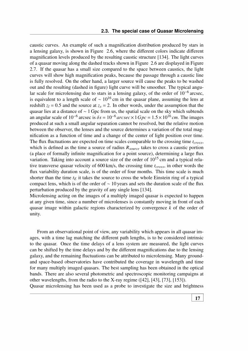
caustic curves. An example of such a magnification distribution produced by stars ina lensing galaxy, is shown in Figure 2.6, where the different colors indicate differentmagnification levels produced by the resulting caustic structure [134]. The light curvesof a quasar moving along the dashed tracks shown in Figure 2.6 are displayed in Figure2.7. If the quasar has a small size compared to the space between caustics, the lightcurves will show high magnification peaks, because the passage through a caustic lineis fully resolved. On the other hand, a larger source will cause the peaks to be washedout and the resulting (dashed in figure) light curve will be smoother. The typical angu-lar scale for microlensing due to stars in a lensing galaxy, of the order of 10−6 arcsec,is equivalent to a length scale of ∼ 1016 cm in the quasar plane, assuming the lens atredshift zl = 0.5 and the source at zs = 2. In other words, under the assumption that thequasar lies at a distance of ∼ 1 Gpc from us, the spatial scale on the sky which subtendsan angular scale of 10−6 arcsec is δs = 10−6 arcsec×1Gpc = 1.5×1016 cm. The imagesproduced at such a small angular separation cannot be resolved, but the relative motionbetween the observer, the lenses and the source determines a variation of the total mag-nification as a function of time and a change of the center of light position over time.The flux fluctuations are expected on time scales comparable to the crossing time tcross,which is defined as the time a source of radius Rsource takes to cross a caustic portion(a place of formally infinite magnification for a point source), determining a large fluxvariation. Taking into account a source size of the order of 1015 cm and a typical rela-tive transverse quasar velocity of 600 km/s, the crossing time tcross, in other words theflux variability duration scale, is of the order of four months. This time scale is muchshorter than the time tE it takes the source to cross the whole Einstein ring of a typicalcompact lens, which is of the order of ∼ 10 years and sets the duration scale of the fluxperturbation produced by the gravity of any single lens [134].Microlensing acting on the images of a multiply imaged quasar is expected to happenat any given time, since a number of microlenses is constantly moving in front of eachquasar image within galactic regions characterized by convergence k of the order ofunity.
From an observational point of view, any variability which appears in all quasar im-ages, with a time lag matching the different path lengths, is to be considered intrinsicto the quasar. Once the time delays of a lens system are measured, the light curvescan be shifted by the time delays and by the different magnifications due to the lensinggalaxy, and the remaining fluctuations can be attributed to microlensing. Many ground-and space-based observatories have contributed the coverage in wavelength and timefor many multiply imaged quasars. The best sampling has been obtained in the opticalbands. There are also several photometric and spectroscopic monitoring campaigns atother wavelengths, from the radio to the X-ray regime ([42], [43], [73], [153]).Quasar microlensing has been used as a probe to investigate the size and brightness
17

Chapter 2. Introduction to AGNs and Quasar Microlensing
Figure 2.6: Caustic magnification pattern in the quasar plane produced by lensing starsin the macro-lens galaxy. The dashed lines crossing the caustics represent three sourcetrajectories. Adapted from [134].
18

2.3. The special case of Quasar Microlensing
Figure 2.7: Light curves from a source crossing the caustic pattern in Figure 2.6. Thefirst panel corresponds to the upper trajectory, the second to the middle trajectory, thethird to the bottom one. Two sets of light curves are displayed. The black line corre-sponds to a small source, the dashed one to a source 10 times larger. The resulting lightcurves are different. Larger sources wash out the microlensing signal as they cross thecaustics, as a consequence of their finite size. Adapted from [134].
19

Chapter 2. Introduction to AGNs and Quasar Microlensing
profile of multiply imaged quasars. This is based on the correlation between the mi-crolensing magnification of a quasar image and the quasar emitting region size, whichdepends on the observed passband [138]. Several authors have looked into the possibil-ity of recovering the brightness profile of a quasar ([7], [58], [59], [179], [118], [104])by observing caustic crossing events in many bands. Several studies have addressedthe question whether the microlensing effect on broad emission lines could be used toresolve the broad line emission regions ([137],[87],[3],[4],[84], [86],[126]).[166],[85] and [152] have considered the variation of the quasar positions in multiplylensed quasars at the caustic crossings, when a bright image pair appears or disappears.The resulting position displacement is estimated to be of the order of 100 microarcsec,observable with high resolution interferometers. Astrometric microlensing, as this tech-nique is referred to, might help estimate the masses of the compact object from a varia-tion in the quasar center of light position. Several works ([165], [122], [24], [23]) werealso able to exclude certain mass values of the compact objects lenses making up thehalo of the lensing galaxy in the particular case of the multiple quasar Q 0957+561. Inall these studies, the absence of microlensing fluctuations with amplitudes larger than∼ 0.1 mag over certain periods of time allowed to exclude that the galaxy halo dark mat-ter consists of compact objects with masses << M�. [52] was, on the other hand, ableto exclude that the galaxy halo in the galaxy of the above lensing system is made up ofobjects with masses 106M � (see also [162]).Flux ratio anomalies are found in lensed quasars. This means that the flux ratios ob-served between the produced images of a multiply imaged quasar do not match the pre-dictions of a simple macrolensing galaxy model. Two different scenarios might providean explanation to the flux-anomaly issue. The first argues that unmodeled substructurenearby the lensing galaxy can change the magnifications of the lensed images [99]. Thiseffect would not depend on the wavelength. On the other hand, [130] suggests that mi-crolensing by compact objects can perturb the observed flux ratios, also demagnifyingthe flux from images emerging in saddlepoint extrema (whose observed flux is oftendemagnified compared to the predicted one) and causing an effect both wavelength- andtime- dependent. In the case microlensing alone is at work, since quasar disks are pre-dicted to emit radiation peaked at longer wavelengths at larger radii [138], it is expectedto observe weaker microlensing signals and flux ratios more similar to the macro-modelvalues when approaching the long wavelength regime of the electromagnetic spectrum.The quadruple quasar HE 0435-1223 [168] shows indeed emission line ratios betweenthe images that match predictions better than the continuum flux ratios, showing thatthe lines are emitted from regions at larger distances from the central engine than thoseemitting the continuum.
20

3Overview of the quasars studied in this
work
3.1 WFI J2033-4723
WFI 2033-4723 is a quadruply imaged quasar, see Fig. 4.4, which was discovered by[102]; the four images, B,A1,A2,C are at redshift zQ = 1.66 and have a maximum angu-lar separation of 2.53 ′′. A Hubble Space Telescope (HST) image of the quasar, adaptedfrom [158], is shown in Fig. 3.1. [102] defined the system as an interesting target formicrolensing studies, since the system flux ratio between the images C and B varied by0.23 mag from the bandpass u to i, while the emission line ratios of the same imagesagreed much better with the macromodel predictions than the ratios corresponding tothe continuum and broadband filters. The emission line ratios suggest that the anoma-lous flux ratio between images C and B in the blue is caused primarily by microlensinginduced perturbations rather than unmodeled substructure in the lensing potential. [41]found that the lens galaxy spectrum is consistent with an elliptical or lenticular galaxytemplate at redshift zL = 0.661± 0.001. The lensing galaxy is a member of a groupwith at least 6 galaxies, whose distance from the lens is at most 20 ′′ [102]. [158] de-termined the time delays between the quasar components to be ∆tB−C = 62.6+4.1
−2.3 daysand ∆tB−A = 35.5± 1.4 days between C and B, and A and B, respectively. The label Aindicates the combination of images A1 and A2. Since A1 and A2 are predicted to havea negligible relative time delay, they are treated as a blend by [158].
3.2 HE 0047-1756
The quasar HE 0047-1756, see Fig. 4.5, was discovered in the Hamburg quasar sur-vey (ESO) at the Magellan 6.5 m telescopes on Cerro Las Campanas, Chile ([170],[123], [169],[172]). This survey used spectra to search for quasars over the entire south-ern sky. An HST image of the double quasar, adapted from [21], is shown in Fig. 3.2.[172] found that the quasar was in fact a lensed system, with identical redshifts of the
21

Chapter 3. Overview of the quasars studied in this work
Figure 3.1: HST NICMOS2 image of quasar WFI 2033-4723, taken in the F160W band.This image has a total exposure time of 46 minutes. North is up and East to the left. Thefield of view is of 4 arcsec.
22

3.2. HE 0047-1756
two images, similar emission line profiles, with a galaxy located between the two com-ponents, and a partial Near Infrared (NIR) Einstein ring. The two observable imageswere separated by ∆θ = 1.44 ′′ and the quasar redshift was estimated at zQ = 1.67. Theyreported a flux ratio for the two components of roughly 3.5 to 1 that slightly dependedon wavelength. The emission line ratio differed from that in the continuum. They at-tributed these small differences to microlensing. However, spectral variability and timedelay effects could not be ruled out. The lensing galaxy, discovered by [172] usingthe Magellan 6.5 m telescopes, is at redshift zL = 0.408 according to [107] (see also[41]). The lens galaxy spectrum matched well with an elliptical galaxy template ([107],[41]). The time delay has not been measured yet. The time delay is a strong increasingfunction of the lensing galaxy redshift and is predicted to be of 32.1 days at zlens = 0.6[172].
Figure 3.2: HST NICMOS2 image of quasar HE 0047-1756.
23
Chapter 3. Overview of the quasars studied in this work
3.3 Q 2237+0305: Huchra’s lens
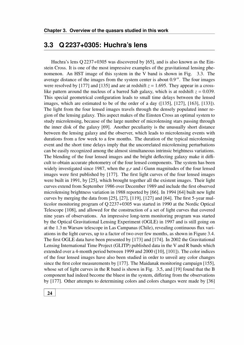
Huchra’s lens Q 2237+0305 was discovered by [65], and is also known as the Ein-stein Cross. It is one of the most impressive examples of the gravitational lensing phe-nomenon. An HST image of this system in the V band is shown in Fig. 3.3. Theaverage distance of the images from the system center is about 0.9 ′′. The four imageswere resolved by [177] and [135] and are at redshift z = 1.695. They appear in a cross-like pattern around the nucleus of a barred Sab galaxy, which is at redshift z = 0.039.This special geometrical configuration leads to small time delays between the lensedimages, which are estimated to be of the order of a day ([135], [127], [163], [133]).The light from the four lensed images travels through the densely populated inner re-gion of the lensing galaxy. This aspect makes of the Einsten Cross an optimal system tostudy microlensing, because of the large number of microlensing stars passing throughthe inner disk of the galaxy [69]. Another peculiarity is the unusually short distancebetween the lensing galaxy and the observer, which leads to microlensing events withdurations from a few week to a few months. The duration of the typical microlensingevent and the short time delays imply that the uncorrelated microlensing perturbationscan be easily recognized among the almost simultaneous intrinsic brightness variations.The blending of the four lensed images and the bright deflecting galaxy make it diffi-cult to obtain accurate photometry of the four lensed components. The system has beenwidely investigated since 1987, when the g,r and i Gunn magnitudes of the four lensedimages were first published by [177]. The first light curves of the four lensed imageswere built in 1991, by [25], which brought together all the existent images. Their lightcurves extend from September 1986 over December 1989 and include the first observedmicrolensing brightness variation in 1988 reported by [66]. In 1994 [64] built new lightcurves by merging the data from [25], [27], [119], [127] and [64]. The first 5-year mul-ticolor monitoring program of Q 2237+0305 was started in 1990 at the Nordic OpticalTelescope [108], and allowed for the construction of a set of light curves that coverednine years of observations. An impressive long-term monitoring program was startedby the Optical Gravitational Lensing Experiment (OGLE) in 1997 and is still going onat the 1.3 m Warsaw telescope in Las Campanas (Chile), revealing continuous flux vari-ations in the light curves, up to a factor of two over few months, as shown in Figure 3.4.The first OGLE data have been presented by [173] and [174]. In 2002 the GravitationalLensing International Time Project (GLITP) published data in the V and R bands whichextended over a 4-month period between 1999 and 2000 ([10], [101]). The color indicesof the four lensed images have also been studied in order to unveil any color changessince the first color measurements by [177]. The Maidanak monitoring campaign [155],whose set of light curves in the R band is shown in Fig. 3.5, and [19] found that the Bcomponent had indeed become the bluest in the system, differing from the observationsby [177]. Other attempts to determining colors and colors changes were made by [36]
24

3.3. Q 2237+0305: Huchra’s lens
and [37], which found significant color variations, and by [156]. A great amount of ob-servations in photometric bands different than the optical range have also been collected,at 20 cm and 3.6 cm [47], in the near and mid infrared ([105], [6]) and at the emissionlines wavelenghts ([49], [119], [31], [87], [129], [42]). Moderate microlensing pertur-bations have been found in these spectral bands, which indicates that the infrared, radioand emission lines regions are larger than the optical continuum emission region. Long-term spectrophotometric monitoring has been conducted at the Very Large Telescopeover three years from October 2004 to December 2007 to constrain the energy profileof the quasar ( [40],[42], [141]). These data showed that the continuum and the broadline region are microlensed. Observations in the UV bands with the HST [15] and in theX-ray regime with the Chandra X-ray Observatory [29] respectively provided accuraterelative astrometry of the components and the estimate of the time delay between theA and B components of 2.7 hours. Several attempts to determine the time delays fromground based observations in the visual wavelengths have also been published. [154]provided the first direct measurements of time delays from optical ground-based data,namely τAB ≈ −6, τCA ≈ 35 and τDA ≈ 2 hours. [77], on the other hand, considered thepossibility of measuring the time delays between the components of the Einstein Crossand showed the impossibility of unambiguously determining the time delays betweenthe lensed components of Q 2237+0305 by making use of ground-based optical datataken with telescopes of ≈ 1.5 m.[164],[175],[178], [72], [11] and [98] showed, by comparing observed light curvesand simulations, that the continuum emission region of the quasar is of the order of∼ 1015 cm. Thanks to a spectrophotometric monitoring of the quasar over a long periodof time, [40] could show that the accretion disk of Q 2237+0305 is consistent with aShakura-Sunyaev accretion disk [138]. In particular, they showed that the microlensingsignal in several bands becomes stronger moving towards shorter wavelengths, an effectoriginally predicted by [161].
25

Chapter 3. Overview of the quasars studied in this work
Figure 3.3: The gravitational lens Q 2237+0305 observed with the HST in the V-band.Adapted from R. W. Schmidt (2000).
26

3.3. Q 2237+0305: Huchra’s lens
Figu
re3.
4:L
ight
curv
esfo
rth
egr
avita
tiona
lsys
tem
Q22
37+
0305
obse
rved
byth
eO
GL
E-I
II(h
ttp://
ogle
.ast
rouw
.edu
.pl/)
mon
itori
ngca
mpa
ign
inth
eV
band
.
27

Chapter 3. Overview of the quasars studied in this work
Figu
re3.
5:L
ight
curv
esfo
rth
egr
avita
tiona
lsy
stem
Q22
37+
0305
obse
rved
byth
eM
AID
AN
AK
mon
itori
ngca
mpa
ign
from
1997
inth
eR
band
.Lig
htcu
rves
prio
rto
1997
have
been
obta
ined
byjo
inin
gup
alre
ady
exis
ting
obse
rvat
ions
.Fro
mht
tp://
ww
w.a
stro
n.kh
arko
v.ua
/dip
/mai
ndep
.htm
.
28

4The MiNDSTEp collaboration and data
acquisition
4.1 MiNDSTEp: Objectives and first results
The MiNDSTEp consortium (Microlensing network for the detection of small ter-restrial exoplanets) is the largest European/Eurasian collaboration which monitors on-going gravitational microlensing events. It aims at the investigation of the nature ofthe population of planets down to Earth mass in the Milky Way. The telescope net-work, including in 2008 only the Danish 1.5 m telescope at ESO LA Silla (Chile), hasbeen expanded to involve the two MONET 1.2 m telescopes at McDonald Observatory(Texas, USA) and the South African Astronomical Observatory. MiNDSTEp relies onmicrolensing surveys as OGLE and MOA (Microlensing Observations in Astrophysics,New Zealand) and realizes by itself the further steps of follow up and monitoring.Quasar microlensing is one of the other projects, other than exoplanetary microlensing,carried out by MiNDSTEp. Five different lensed quasar were observed by the collabo-ration at the Danish 1.5 m telescope.The Danish 1.54 m telescope has been at La Silla since 1979, see Fig. 4.1. It isnow equipped with the Danish Faint Object Spectrograph and Camera (DFOSC). Thetelescope has allowed several first discoveries. It has also produced many impressiveastronomical images. Some important facts regarding the Danish telescope are sum-marized in Fig. 4.2. The observations of quasars WFI 2033-4723, HE 0047-1756 andQ 2237+0305, from 2008 to 2012, are matter of this thesis; the observations of HE 0435-1223 and UM673 have been published in two papers by [125] and [124]. In the firstpaper, they presented the VRi photometric observations of the quadruply imaged quasarHE 0435-1223, with the aim to study magnitudes and colors of each lensed componentas a function of time. The target was monitored during the seasons 2008 and 2009and analyzed with two different techniques, differential image photometry and PointSpread Function (PSF) fitting. They found a significant decrease in flux by 0.2-0.4 magof the lensed components in all photometric bands, together with a significant increase
29

Chapter 4. The MiNDSTEp collaboration and data acquisition
of ≈ 0.05− 0.015 mag of the colour indices V −R and R− i between the two seasons.They concluded by arguing that the flux and colour variations are very likely causedby intrinsic variations of the quasar between the observing seasons, with microlensingaffecting probably the brightest A component, which showed the largest shift in color.The flux and color variations of the doubly lensed quasar UM673 as a function of timeare analyzed in the second paper. The observations were carried out during four seasonsfrom 2008 to 2011 in the photometric bands VRi. Data were reduced by making use ofthe PSF fitting alongside with aperture photometry. The brightest lensed quasar compo-nent A showed some flux decrease between 2008 and 2009 in all bands of the order of≈ 0.1 mag, followed by an increase of the order of ≈ 0.1 mag during the following sea-sons. The colour index variations found between the seasons were smaller than thosefound by previous studies.
Figure 4.1: The Milky Way and the Magellanic Clouds above the Danish telescopedome, on the right in the picture. From http://www.eso.org/public/images/.
30

4.1. MiNDSTEp: Objectives and first results
Figure 4.2: Table summarizing the main properties of the Danish telescope. Adaptedfrom (http://www.eso.org/public/.)
31

Chapter 4. The MiNDSTEp collaboration and data acquisition
4.2 Data acquisition
The observations of the lensed quasars WFI 2033-4723, HE 0047-1756 and Q 2237+0305 were obtained in the V and R bands with the 1.54 m Danish telescope at ESO/LaSilla, Chile, by the MiNDSTEp (Microlensing network for the detection of small ter-restrial exoplanets, [35]) quasar monitoring campaign. The observations were collectedduring five observing seasons, from 2008 to 2012. The quasars were observed within thefollowing temporal intervals: from June 5 to October 4 2008, from June 19 to Septem-ber 18 2009, from May 9 to August 21 2010, from June 11 to August 31 2011 and fromJuly 16 to September 16 2012. During these periods we observed the quasars everytwo days, weather permitting, in the V and R filters of the Bessel system. The quasarswere observed on average three times per night. WFI 2033-4723 was observed with anexposure time of 180 s in V and R, except for a small number of images, with longer ex-posure times of 300 s and 600 s, at the start of 2008. Exposure times for HE 0047-1756varied from 180 s in both filters during the first two seasons to 240 s in V and 210 s inR during the last three years. A few images in both bands at the start of the first seasonwere taken with exposure times of 300 s and 600 s. Exposure times for Q 2237+0305,were of 180 s in both filters for most part of the observing campaign. A few images inboth bands at the start of the first season were taken with exposure times of 300 s and600 s and in June 2009 with exposure times of 200 s.
The median seeing of the observations was ≈ 1.3 ′′, taking into account both filtersand all data. The observations were made with the DFOSC imager, shown in Fig. 4.3,with a pixel scale of 0.39 ′′. The full field of view (FOV) was 13.7 arcmin × 13.7 arcmin.A section of the FOV centred on the quasars is shown in Figs. 4.4, 4.5 and 4.6.
32

4.2. Data acquisition
Figure 4.3: The Danish Faint Object Spectrograph and Camera (DFOSC). Itconsists of a collimator and a camera, between which are a filter and agrism wheel. An aperture wheel is at the telescope focus. Adapted fromhttp://www.ls.eso.org/sci/facilities/lasilla/.
33

Chapter 4. The MiNDSTEp collaboration and data acquisition
Figure 4.4: V-band image of WFI 2033-4723 obtained by stacking the 14 best seeingand sky background images (V-band template image). The quasar and the star, whichwe use both as a constant reference and a PSF model, are labelled. The four lensedquasar components are enlarged in the darker box. The field size is 9.7 arcmin × 9.5arcmin. The stamps used for the kernel computation are defined as 17-pixel squares(See Sect. 6.3.2).
34

4.2. Data acquisition
Figure 4.5: V-band image of HE 0047-1756 obtained by stacking the 10 best seeingand sky background images (V-band template image). The quasar and the stars that weuse as a constant reference and PSF model are labelled. The double lensed quasar isenlarged in the darker box. The field size is 8.5 arcmin × 8.8 arcmin. The stamps usedfor the kernel computation are defined as 17-pixel squares (See Sect. 6.3.2).
35

Chapter 4. The MiNDSTEp collaboration and data acquisition
Figure 4.6: V-band image of Q 2237+0305 obtained by stacking the 7 best seeing andsky background images (V-band template image). The quasar and the stars that we useas a constant reference and PSF models are labelled. The alpha star, used in [25] forphotometric calibration, is also shown. The quasar is enlarged in the darker box. Thefield size is 9.7 arcmin × 10 arcmin. The stamps used for the kernel computation aredefined as 17-pixel squares (See Sect. 6.3.2).
36
5Data Reduction
5.1 Data storage
All the images have been downloaded from the MiNDSTEp wiki page, where all thedata taken at the Danish telescope are available, apart from the frames acquired duringthe year 2012, which were stored on an external hard drive enclosure at the end of theobserving run at La Silla in August/September 2012. Before proceeding with furtheranalysis, all the nightly frames have been flat fielded, bias subtracted, corrected for badcolumns, aligned to a common reference frame, trimmed at the edges in order to enclosethe same region, and finally, the images taken during a single night have been mediancombined, in order to improve their signal-to-noise ratio and remove cosmic rays.
5.2 Flat Fielding and bias correction
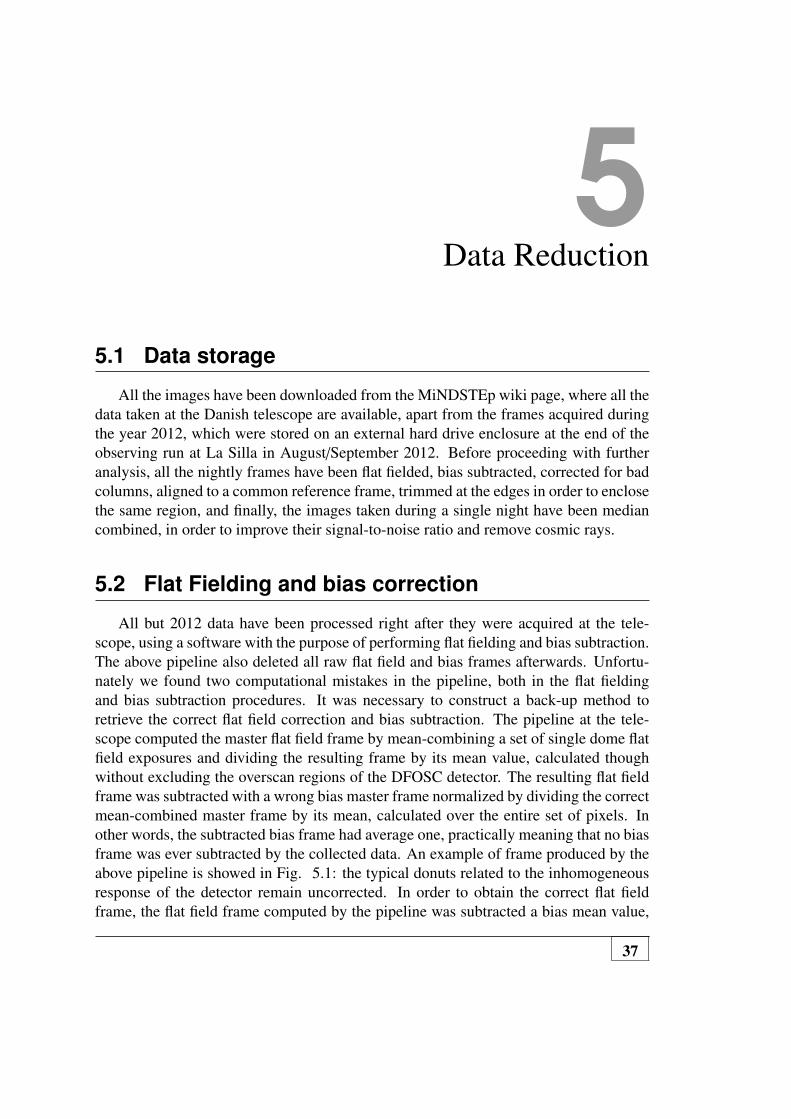
All but 2012 data have been processed right after they were acquired at the tele-scope, using a software with the purpose of performing flat fielding and bias subtraction.The above pipeline also deleted all raw flat field and bias frames afterwards. Unfortu-nately we found two computational mistakes in the pipeline, both in the flat fieldingand bias subtraction procedures. It was necessary to construct a back-up method toretrieve the correct flat field correction and bias subtraction. The pipeline at the tele-scope computed the master flat field frame by mean-combining a set of single dome flatfield exposures and dividing the resulting frame by its mean value, calculated thoughwithout excluding the overscan regions of the DFOSC detector. The resulting flat fieldframe was subtracted with a wrong bias master frame normalized by dividing the correctmean-combined master frame by its mean, calculated over the entire set of pixels. Inother words, the subtracted bias frame had average one, practically meaning that no biasframe was ever subtracted by the collected data. An example of frame produced by theabove pipeline is showed in Fig. 5.1: the typical donuts related to the inhomogeneousresponse of the detector remain uncorrected. In order to obtain the correct flat fieldframe, the flat field frame computed by the pipeline was subtracted a bias mean value,
37

Chapter 5. Data Reduction
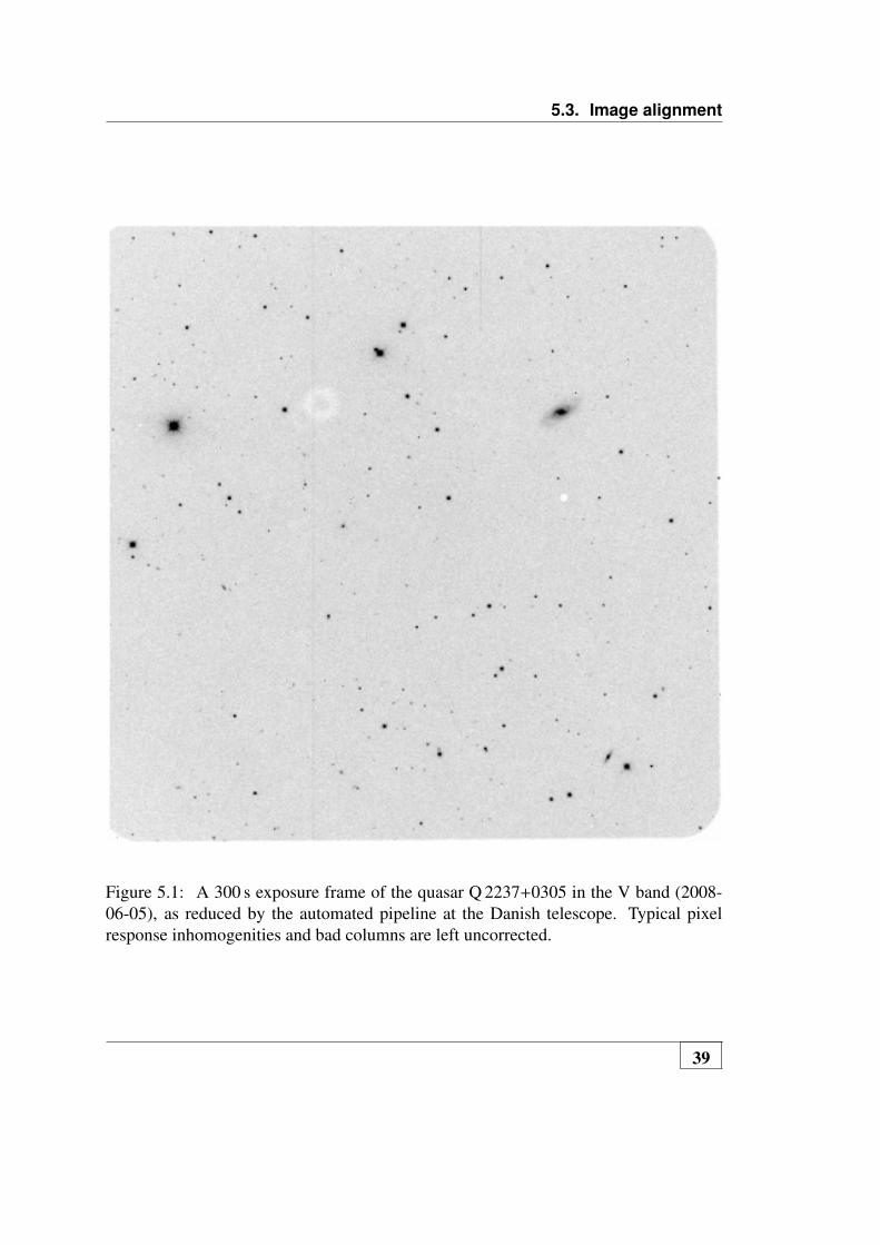
calculated from the overscan regions, and then divided by its mean calculated over asmaller region of responsive pixels. The flat field master frames for the year 2012 wereinstead computed by mean-combining the available dome flat field exposures and di-viding them by the mean of the resulting frame, after having subtracted from each ofthem the corresponding bias master frame. All the science images (except for 2012)were then subtracted their mean bias value (from the overscan regions) and divided bythe retrieved flat field master frames. Bad columns were replaced with the appropriatemedian of surrounding pixels. An example of science image, processed as describedabove, is shown in Fig. 5.2. As it can be seen, the chip response inhomogenities andthe bad column features have been now correctly treated. Science frames collected in2012 were instead subtracted the corresponding bias master frame and divided by theappropriate flat field master frame.
5.3 Image alignment
Before subtraction, all images need to be astrometrically aligned to a referenceframe. The reference image of a given source is an image in a given passband char-acterized by a very good seeing and low sky background. All the other images of thesame quasar are registered onto the reference coordinate grid, also when taken in a dif-ferent photometric band. This is carried out using the ISIS1 package by C. Alard ([9],[8]). The astrometric alignment routine of this package efficiently identifies referencestars in the field and performs a two-dimensional polynomial mapping to the referenceimage. We chose a polynomial transformation of order 2 to remove the shifts and smallrotations between the images. In the case of WFI 2033-4723, the average residuals cor-responding to the astrometric transform along the x- and y-axes were of the order of0.1 pixel and the mapping was computed using on average ≈ 275 objects. The astromet-ric transforms corresponding to HE 0047-1756 were characterized by average residualsof the order of 0.2 pixel and obtained taking into account on average ≈ 220 objects. Inthe case of Q 2237+0305, the average residuals were of the order of 0.18 pixels and 164objects were identified on average for the tranform computations. Image resamplingwas performed through bicubic splines. All images of a given night for the whole dataset were trimmed at the edges to contain the same region and median combined to im-prove the signal-to-noise ratio and correct for cosmic rays. The combination was madeby using the IRAF routine IMCOMBINE, which combined images with different ex-posure times and sky background levels by carrying out an appropriate scaling and byadding a background constant before stacking them. After discarding images with highsky background, disturbed by moonlight, clouds, bad tracking and bad columns, we fi-nally used 85 nights for WFI 2033-4723, 108 nights for HE 0047-1756 and 57 nights for
1http://www2.iap.fr/users/alard/package.html
38
5.3. Image alignment
Figure 5.1: A 300 s exposure frame of the quasar Q 2237+0305 in the V band (2008-06-05), as reduced by the automated pipeline at the Danish telescope. Typical pixelresponse inhomogenities and bad columns are left uncorrected.
39
Chapter 5. Data Reduction
Figure 5.2: A 300 s exposure frame of the quasar Q 2237+0305 in the V band (2008-06-05), as reduced by correcting the computational mistakes found in the Danish telescopereduction pipeline. Typical pixel response inhomogenities and bad columns are nowcorrected.
40

5.3. Image alignment
Q 2237+0305 in five years. V- and R-band images were not always both available at agiven night. The images were finally ready for applying the differential image subtrac-tion technique and proceeding to further analysis.
41


6Theory and Practice of Differential Image
Analysis
6.1 Differential Image Analysis applied to lensed quasars:an overview
As was shown in the case of Huchra’s lens ([173],[10],[101], [153]), an optimal pro-cedure to perform photometry in the case of a multiply imaged quasar is the differenceimage analysis method (DIA) proposed by [9] and [8]. The basic principle is to use ahigh signal-to-noise template image, with good seeing and low sky background, whichis subtracted from every other target frame in the data set. Since the contribution fromthe galaxy, which is not expected to vary, is removed in the subtracted images, modelingthe galaxy light distribution is no longer required. This greatly simplifies the photom-etry of the quasars. Before proceeding to subtraction, each pair of images needs to beastrometrically and photometrically aligned. After subtraction, relative photometry canbe carried out. This is achieved by building a model for the quasar images with a blendof known PSFs making use of the HST astrometry of the quasar.The idea of Alard & Lupton [9] is to compute the best-fit spatially non-varying convo-lution kernel, which degrades the template PSF into that of the target frame and simul-taneously matches atmospheric extinction and exposure time. The authors show that bydecomposing the kernel as a linear combination of N basis functions, its computationcan be as simple as determining a finite number of kernel coefficients. The coefficientsare found by solving a linear system of equations containing various moments of the twoinput images. The chosen convolution kernel is a sum of several Gaussians, which aremultiplied by polynomials to model the possible asymmetry of the kernel. The Gaussianwidths depend on the relative sizes of the PSF in the template and target frame. Alard[8] extended this technique to the case of a kernel that varies across the chip. Assum-ing that the amplitudes of the kernel components are polynomial functions of the pixelcoordinates of order n, the number of kernel coefficients of each component becomes(n+1)(n+2)/2 larger than in the constant kernel problem.
43

Chapter 6. Theory and Practice of Differential Image Analysis
6.2 Full theory of the Alard&Lupton image subtrac-tion method with constant and space-varying con-volution kernels
In their first paper, published in 1998, [9] presented a method for optimal subtractionof two images collected with different observing conditions (i.e. seeing, exposure time,atmospheric extinction) in order to provide a new and fast method to analyze variabilityof astronomical sources. After choosing the best signal-to-noise, seeing and low skybackground image (template) and registering the template and the target image to thesame coordinate grid, the method carries out the matching between the two differentPSFs. This approach consists of finding the least-square solution for the convolutionkernel K(u,v), with u and v coordinates in the kernel coordinate space, which convolvesthe template T(x,y), with x and y coordinates in the image coordinate space, to give, asa result, the target frame I(x,y) according to the following equation
T (x,y)⊗K(u,v) = I(x,y). (6.1)
When decomposing the kernel as a sum of k basis functions, the above problembecomes a linear least-squares problem. By using a kernel of the form:
K(u,v) =∑
kakBk(u,v), (6.2)
the squared difference between T (x,y)⊗K(u,v) and I(x,y) is minimized by solvingthe following linear system for the unknown coefficients ak
Ma = V, (6.3)
where
Mi, j =
∫Ci(x,y)
C j(x,y)σ2(x,y)
dxdy (6.4)
Vi =
∫I(x,y)
Ci(x,y)σ2(x,y)
dxdy (6.5)
Ci(x,y) = T (x,y)⊗Bi(u,v). (6.6)
By looking for a kernel solution with least-squares, the authors have implicitly ap-proximated the image Poisson statistics by a Gaussian distribution σ(x,y) and assumedthat the template noise is negligible. The basis functions are chosen to be Gaussianfunctions of widths σn, modified by a polynomial factor. The kernel decompositionassumes the form:
44

6.2. Full theory of the Alard&Lupton image subtraction method withconstant and space-varying convolution kernels
K(u,v) =∑
n
∑ln
∑mn
ake−
(u2+v2)2σ2
n ulnvmn (6.7)
where 0≤ ln ≤Dn and 0≤ ln +mn ≤Dn, being Dn the degree of the polynomial modi-fying the Gaussian component n. Each component n admits a total of (Dn +1)(Dn +2)/2terms. The value of k is determined by the values of the other indexes n, ln,mn.
In crowded fields, with many stars for modeling the PSF, the fit can be carried outover small regions and the kernel variations can be neglected. On the other hand, in thecase of sparse fields when dealing with quasars or supernovae, the number of objectsneeded to compute the kernel cannot be found in a small area and the kernel variationscannot be ignored. Moreover, by introducing new coefficients in order to solve for thekernel variations, the computing time will increase as the square of the number of thecoefficients. These considerations led Alard to the publication of a second paper, [8], inwhich a method for image subtraction with non-constant kernel solutions is proposed.This allows to obtain a solution investing little additional computing time.
To describe the spatial variation of the kernel as a function of the variables x andy, the kernel can be decomposed as a sum of basis functions at each spatial point (x,y).Hence, the coefficients ak will become functions of (x,y). Assuming that the coefficientsak are polynomial functions of degree dk
ak(x,y) =∑i, j
bki, jx
iy j, (6.8)
the resulting kernel can then be written as:
K(u,v)x,y =∑
n
∑ln
∑mn
∑i, j
bki, jx
iy je−
(u2+v2)2σ2
n ulnvmn , (6.9)
where the notation is the same as in Eq. 6.7, 0 ≤ i ≤ dk and 0 ≤ i + j ≤ dk.In this case, finding a least square solution to the Eq. 6.1 is equivalent to solving
the following linear system for the coefficients bki, j
Mb = V, (6.10)
where the matrix element Mp,q is given by
Mp,q =
∫Wp(x,y)Pp(x,y)Wq(x,y)Pq(x,y)dxdy. (6.11)
45
Chapter 6. Theory and Practice of Differential Image Analysis
The indexes p and q span over the number N of unknown coefficients, (Dn +1)(Dn +
2)(dk + 1)(dk + 2)/4 for each component n. The functions appearing in the matrix aregiven by
Wp(x,y) =T ⊗Bp(x,y)σ(x,y)
=Cp(x,y)σ(x,y)
(6.12)
and
Pp(x,y) = xipy jp . (6.13)
The components of vector V have the form:
Vp =
∫I(x,y)
Wp(x,y)σ(x,y)
Pp(x,y)dxdy. (6.14)
All the above integrals extend over the entire images. By dividing the integrationarea into smaller sub-areas of index r and center (xr,yr), within which the kernel can beconsidered constant, the above matrix becomes
Mp,q =∑
rPp(xr,yr)Pq(xr,yr)
∫Dr
Wp(x,y)Wq(x,y)dxdy (6.15)
and the above vector takes the form
Vp =∑
rPp(xr,yr)
∫Dr
I(x,y)Wp(x,y)σ(x,y)
dxdy. (6.16)
From Eq. 6.4, 6.5, 6.6, 6.15 and 6.16, it can be seen that solving the kernel equationin the case of a spatially-varying kernel can be simply deduced from solving the equa-tions for the constant kernels corresponding to the image sub-areas and summing overthe sub-area solutions. This approximation allows to compute a non-constant kernelsolution with minimum additional computing time.
6.3 Image subtraction in practice
In this thesis image subtraction was carried out with the HOTPAnTS1 software byA. Becker, which is an enhanced and modified version of the [8] method and the corre-sponding implementation software ISIS. This software is given the template image andthe target frames to be processed. In creating the template images, we stacked the frameswith the best seeing and sky background at our disposal. In the case of WFI 2033-4723we computed the median stack of 14 images, both in the V- and R- bands. A similar
1http://www.astro.washington.edu/users/becker/hotpants.html
46

6.3. Image subtraction in practice
0 0.05
0.1 0.15
0.2 0.25
0.3 0.35
0.4 0.45
0 0.5 1 1.5 2
0 1 2 3 4 5
Fract
ion
pixel
V-band
0 0.05
0.1 0.15
0.2 0.25
0.3 0.35
0.4 0.45
0 0.5 1 1.5 2
0 1 2 3 4 5
pixel
R-band
WFI2033-4723
0
0.05
0.1
0.15
0.2
0.25
0.3
0.35
0.4
0.45
0 0.5 1 1.5 2
0 1 2 3 4 5
Fract
ion V-band
0
0.05
0.1
0.15
0.2
0.25
0.3
0.35
0.4
0.45
0 0.5 1 1.5 2
0 1 2 3 4 5
R-band
HE0047-1756
0 0.05
0.1 0.15
0.2 0.25
0.3 0.35
0.4 0.45
0 0.5 1 1.5 2
0 1 2 3 4 5
Fract
ion
σ(arcsec)
V-band
0 0.05
0.1 0.15
0.2 0.25
0.3 0.35
0.4 0.45
0 0.5 1 1.5 2
0 1 2 3 4 5
σ(arcsec)
R-band
Q2237+0305
Figure 6.1: FWHM distributions of a nearby star of WFI 2033-4723 (top), HE 0047-1756 (middle) and Q 2237+0305 (bottom) in filters V (left) and R (right) in terms of thecorresponding Gaussian σ.
47

Chapter 6. Theory and Practice of Differential Image Analysis
Figure 6.2: V-band difference images of WFI 2033-4723 from 2008 to 2012. The cor-responding dates are listed in Table 11.2.
48

6.3. Image subtraction in practice
procedure was carried out in building the template images for HE 0047-1756, for whichwe were able to combine 10 frames in V and 14 frames in R. In the case of Q 2237+0305we used 7 frames in the V-band and 14 frames in the R-band.
6.3.1 HOTPAnTS modus operandiHOTPAnTS divides the frames into square regions, within which smaller regions
called stamps, centered on individual stars, are chosen. The software is also given thelist of stars at the center of the stamps. A kernel solution is derived for each stamp.Thekernel sum is used as a first metric to discard bad stamps. The photometric scalingbetween two images is the sum of the convolution kernel. This result follows from Eq.6.1 and from noticing that the integral of the convolution of two functions is the productof their integrals. In formulas,
∫(T ⊗K)(x,y)dxdy =
∫T (x,y)dxdy
∫K(u,v)dudv =
∫I(x,y)dxdy. (6.17)
From the two rightmost terms it can be concluded that FI = FT KS UM, where FI andFT indicate the flux of a source in the image and template respectively and KS UM is thesum of the kernel.
This can be used to discard variable stars (not suitable for determining the photo-metric alignment between the images) by sigma-clipping outlier stamps from the dis-tribution of the kernel sums. It is useful to have multiple choices in a particular imageregion in case any objects are sigma-clipped. At this stage, another metric is used todiscard bad stamps: after convolution and subtraction, the mean of the distribution ofpixel residuals divided by the estimated pixel variance across each stamp provides anadditional figure of merit to sigma-clip stamps out and replace them with neighboringstars. The constraints on the convolution kernel for each stamp then allow for the fittingof the coordinate dependent amplitudes of the kernel components.
6.3.2 HOTPAnTS implementationAs analytical kernel basis functions we chose three Gaussians, which were modi-
fied by multiplicative polynomials of orders 4, 3 and 2, respectively, with the aim ofmodeling the kernel asymmetries. In general, we chose a narrow Gaussian which var-ied to order 4, a central wider Gaussian which varied at order 3 and a broad Gaussian,which varied at order 2, in the coordinates (u,v) of the kernel space. The values of theGaussian widths σ were computed on the basis of the seeing range of the templates andtarget frames given to HOTPAnTS. For the target frames we computed, in the V and Rbands, the seeing distribution of a star in the quasar neighborhoods. We obtained the
49
Chapter 6. Theory and Practice of Differential Image Analysis
corresponding σ distribution, as shown in Fig. 6.1, making use of the relation betweenthe Full Width at Half Maximum (FWHM) and the σ of a Gaussian profile. The triplet(0.8,1.4,2.3), expressed in pixel units, was a good general choice to build the kernelbasis functions which, convolved with the typical template σ of 1 pixel, reproduced thetypical target frame σ values. These values were hence adopted as our Gaussian widths.The polynomials modeling the spatial variation of the kernel amplitudes were allowedto vary at spatial order 2 in the image space coordinates (x,y). The final number ofstamps differed from case to case since it in general depended on the star distributionin the field. The field characterizing the frames of WFI 2033-4723 was rich with stars,while those corresponding to HE 0047-1756 and Q 2237+0305 were quite sparse. Theconvolution kernel of WFI 2033-4723 was derived by taking into account on average 27stamps in V and 26 in R; on average 8 stamps in V and 10 in R defined the convolutionkernel for HE 0047-1756. In the case of Q 2237+0305, 15 stamps were used on averagein the V-band and 12 in the R-band. The size of the stamps of 17×17 pixels was suchthat it contained the whole star flux profiles. Figs. 4.4, 4.5 and 4.6 show the squaresdefining the stamps that HOTPAnTS selected across all observing seasons in the filtersV and R for the three systems.Additional necessary inputs for the HOTPAnTS software were the target frame andtemplate gain (G) and readout noise (RON). Throughout the years 2008-2011 the in-strumental gain G was 0.76e−/ADU and the readout noise RON was 3.21e−. The Gand RON values changed in 2012 due to an upgrade of the DFOSC detector between2011 and 2012. The values valid for 2012 are G = 0.24e−/ADU and RON = 5.28e−. 2
The gain and RON had to be adjusted appropriately before giving them to HOTPAnTS.Since both the target frames and the templates are in general stacked images, we neededto define an effective G and RON by using standard variance propagation. Starting fromthe following expression for the stacked image
I =
N∑1
Fi× Ii
N, (6.18)
where Ii represents a single exposure, Fi the weights which bring the single expo-sures to a common exposure time and N the number of single exposures, we defined thecorresponding variance σI
2, in which we arranged terms in order to isolate the effec-tive readout noise and photon noise components. Another adjustable set of parameterswas the model for the sky background, which was selected to be an additive constant.The output by HOTPAnTS was the difference image, with the seeing of the current tar-get frame and the photometric scale of the template, and the corresponding noise map.Fig. 6.2 shows the sequence of difference images for WFI 2033-4723 in filter V .
2The G and RON values for 2012 are kindly provided by Noe Kains.
50

6.4. Photometry
6.4 Photometry
Photometry on the difference images was performed using the GALFIT software(version 2.0.3, [115]). The GALFIT software was modified to allow the fitting of ablend of PSFs with fixed relative separations and linear fluxes. We used it to analyzethe lensed quasars in the original images and in the difference images. This was doneas follows:
1. A nearby star was chosen as a PSF model (the chosen stars are labelled as PSFin Figs. 4.4, 4.5 and 4.6). We used only one star since we noticed a remark-able variation of the PSF through the field and decided to select the closest brightenough, isolated and not saturated star in the neighborhoods. The GALFIT soft-ware normalized the star chosen as PSF so that any variability was not an issue.The PSF was built by extracting a 17×17 pixel box surrounding the star; the PSFwas sky-subtracted and centered at pixel (9,9) according to the formula reportedin the GALFIT manual. We used the IRAF routine IMSHIFT for shifting the PSFcenter.
2. Using the PSF model, the quasar positions were determined from the originalstacked images and the templates with GALFIT by keeping all the quasar fluxesand the position of only one of the lensed quasar images as free parameters. Thesky background values at the quasar position were fixed to median values esti-mated from 51×51 pixel empty regions nearby the quasar. The positions of theremaining lensed quasar components relative to the free quasar component werekept fixed at the values shown in Table 6.1, obtained from the CASTLES 3 webpage (C.S. Kochanek, E.E. Falco, C. Impey, J. Lehar, B. McLeod, H.-W. Rix) anddetermined using Hubble Space Telescope data.
In the case of the original stacked images and template images, since in generalthey contained a number of single exposures with different exposure times, we letGALFIT build the appropriate corresponding sigma image by providing it withthe equivalent GAIN and RDNOISE of the frames, since GALFIT was only ableto correctly compute the noise image for a stack of N images with identical gain,readout noise and exposure time.
3. In the data of WFI 2033-4723 and HE 0047-1756 we could not significantly de-tect the lensing galaxies. Our positions were therefore minimally affected by thepresence of the V ≈ 21 mag (WFI 2033-4723) and V ≈ 22.5 mag (HE 0047-1756)lensing galaxy and in these cases the above description of the determination ofthe quasar positions was used. Keeping fixed the nightly lensed quasar positions
3http://www.cfa.harvard.edu/castles/
51

Chapter 6. Theory and Practice of Differential Image Analysis
Table 6.1: HST relative astrometry of WFI 2033-4723, HE 0047-1756 andQ 2237+0305 images, obtained from the CASTLES webpage.
WFI2033A1 A2 B C
RA(”) 2.196±0.003 −1.482±0.003 0 −2.114±0.003DEC(”) 1.261±0.003 1.376±0.003 0 −0.277±0.003
HE0047A B
RA(”) 0 0.232±0.003DEC(”) 0 −1.408±0.003
Q2237A B C D
RA(”) 0 0.673±0.000 0.635±0.000 −0.866±0.000DEC(”) 0 1.697±0.000 1.210±0.000 0.528±0.000
obtained above, we determined the fluxes at the position of the quasar images inthe difference images. The GALFIT software was allowed to fit negative fluxes aswell in order to process the differential fluxes of the subtracted images. In the caseof Q 2237+0305, on the other hand, we dealt with a lensing galaxy with an opticalaverage magnitude of ≈ 15 mag. In this case, we opted for fitting the quasar posi-tions on the difference image residual fluxes instead of using the original stackedimages.Then we determined the fluxes in the difference images at fixed centroids of thequasar images, which were computed by yearly averaging the best fit positions ofthe quasar images obtained from the procedure above. The result for all quasarswere the difference fluxes between the epoch considered and the template image.For the difference image photometry with GALFIT the output noise map fromHOTPAnTS was used.
The robustness of the method just described has been tested also by computingthe light curves of the four components of quasar HE 0435-1223 ([169], [171]),observed by MiNDSTEp and already published by [125], and comparing themwith the results by [26] (in the R band). The consistency of the four light curves,obtained with two different telescopes and two different methods, is very good,as shown in Fig. 6.3, with an average weighted root mean square deviationof rms = 1.36σ. A similar test has been done by computing with this methodthe light curves of quasar UM673 ([90], [146], [145]), [142], [39]), observedby MiNDSTEp and published by [124], and comparing the results for the twocomponents with the results obtained in filters V and R by [75]. The averageweighted root mean square deviation was rms = 1.6σ.
52

6.4. Photometry
0
0.2
0.4
0.6
0.8
1
1.2
1.4
1.6
1.8
52500 53000 53500 54000 54500 55000 55500
Rela
tive R
Magnit
ud
e
MJD
D
A
B
C
Present work APresent work BPresent work CPresent work D
Courbin et al. (2011) ACourbin et al. (2011) BCourbin et al. (2011) CCourbin et al. (2011) D
Figure 6.3: The R light curves of the four components of the quasar HE 0435-1223 as ofthe present work are plotted as a function of the Modified Julian Date (MJD) on top ofthe corresponding light curves as found by [26] (from 2004 to 2010) with the purposeof showing the consistency of the obtained light curves. The match is only possible inthe time span enclosed between the two dashed lines, which corresponds to years 2009and 2010.
53
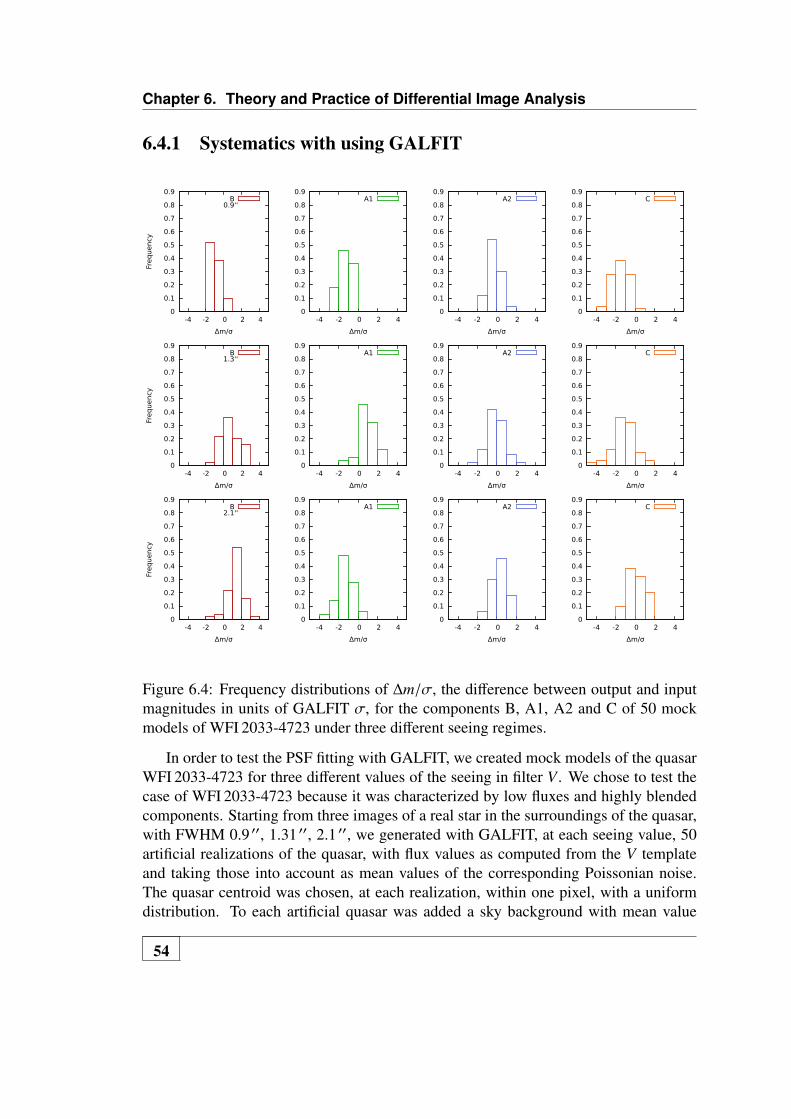
Chapter 6. Theory and Practice of Differential Image Analysis
6.4.1 Systematics with using GALFIT
0
0.1
0.2
0.3
0.4
0.5
0.6
0.7
0.8
0.9
-4 -2 0 2 4
Freq
uency
Δm/σ
0.9''B
0
0.1
0.2
0.3
0.4
0.5
0.6
0.7
0.8
0.9
-4 -2 0 2 4
Δm/σ
A1
0
0.1
0.2
0.3
0.4
0.5
0.6
0.7
0.8
0.9
-4 -2 0 2 4
Δm/σ
A2
0
0.1
0.2
0.3
0.4
0.5
0.6
0.7
0.8
0.9
-4 -2 0 2 4
Δm/σ
C
0
0.1
0.2
0.3
0.4
0.5
0.6
0.7
0.8
0.9
-4 -2 0 2 4
Freq
uency
Δm/σ
1.3''B
0
0.1
0.2
0.3
0.4
0.5
0.6
0.7
0.8
0.9
-4 -2 0 2 4
Δm/σ
A1
0
0.1
0.2
0.3
0.4
0.5
0.6
0.7
0.8
0.9
-4 -2 0 2 4
Δm/σ
A2
0
0.1
0.2
0.3
0.4
0.5
0.6
0.7
0.8
0.9
-4 -2 0 2 4
Δm/σ
C
0
0.1
0.2
0.3
0.4
0.5
0.6
0.7
0.8
0.9
-4 -2 0 2 4
Freq
uency
Δm/σ
2.1''B
0
0.1
0.2
0.3
0.4
0.5
0.6
0.7
0.8
0.9
-4 -2 0 2 4
Δm/σ
A1
0
0.1
0.2
0.3
0.4
0.5
0.6
0.7
0.8
0.9
-4 -2 0 2 4
Δm/σ
A2
0
0.1
0.2
0.3
0.4
0.5
0.6
0.7
0.8
0.9
-4 -2 0 2 4
Δm/σ
C
Figure 6.4: Frequency distributions of ∆m/σ, the difference between output and inputmagnitudes in units of GALFIT σ, for the components B, A1, A2 and C of 50 mockmodels of WFI 2033-4723 under three different seeing regimes.
In order to test the PSF fitting with GALFIT, we created mock models of the quasarWFI 2033-4723 for three different values of the seeing in filter V . We chose to test thecase of WFI 2033-4723 because it was characterized by low fluxes and highly blendedcomponents. Starting from three images of a real star in the surroundings of the quasar,with FWHM 0.9 ′′, 1.31 ′′, 2.1 ′′, we generated with GALFIT, at each seeing value, 50artificial realizations of the quasar, with flux values as computed from the V templateand taking those into account as mean values of the corresponding Poissonian noise.The quasar centroid was chosen, at each realization, within one pixel, with a uniformdistribution. To each artificial quasar was added a sky background with mean value
54

6.4. Photometry
as computed from the V template, including Poissonian noise, and a Gaussian readoutnoise realization obtained with the IRAF routine MKNOISE. No lensing galaxy wasincluded in these simulations. The photometry of the artificial models was then carriedout with GALFIT, choosing a PSF close to that used in building the artificial models.Fig. 6.4 shows the distribution of the ratio ∆mag/σ, which represents the differencebetween the GALFIT output flux and the known input flux, in units of GALFIT sigmas,for the quasar images and for the three values of seeing. The majority of realizationslies between ∆mag/σ ≈ 0− 2 with minor tails at ∆mag/σ ≈ 3. The effects leading tothe systematic discrepancy between the input and output fluxes were determined by thedifferences between the PSF of the quasar and the PSF chosen to model it. The averagemagnitude discrepancy in the most frequent seeing regime did not exceed 0.02 mag,negligible for the purposes of this thesis.
55

7WFI 2033-4723
In what follows we report the results obtained for the quasar WFI 2033-4723. Thismaterial has already been published in the paper [2] listed in the List of Publications.
7.1 Light curves of the quasar WFI 2033-4723
Figure 7.1 shows the light curves for the quasar WFI 2033-4723 components B, A1,A2, C and the constant star in Fig. 4.4 in filters V and R. The light curves are computedby using instrumental magnitudes, which are defined as:
mX = −2.5× log10((∆FX + FX,T )/FX,Re f ) (7.1)
where ∆FX is the flux difference of the quasar components in the subtracted image,which has the photometric scale of the template, FX,T is the corresponding flux in thetemplate and FX,Re f that of the constant reference stars, marked in Figs. 4.4, 4.5 and4.6, in the X band. Instrumental colors are defined accordingly from the magnitudes.The individual data points composing the light curves are also listed in Table 11.2. Thelight curves of images B (filled dots), A1 (asterisks), A2 (squares), C (filled diamonds)are shown in red, green, orange and blue, respectively, as a function of the ModifiedJulian Date (MJD). The quoted error bars were determined by the GALFIT software,as explained in paragraph 6.4. The illustrated photometric data of the quasar compo-nents have been shifted in accordance with the time delays published by [158], namely∆tB−C = 62.6+4.1
−2.3 days and ∆tB−A = 35.5±1.4 days, with image B leading. ComponentsB, A1, A2, C became brighter in 2009 and dimmer again across the remaining seasons,showing an overall magnitude variation of ≈ 0.6 mag in filter V and ≈ 0.5 mag in filter R.We list in Table 7.1 the average magnitudes, computed within each season, for a moredetailed picture of the brightness evolution of the four images. The quoted error barsare standard deviations computed within each season. Fig. 7.2 is intended to reveal anydifferences between the variation of the four lensed components.
57

Chapter 7. WFI 2033-4723
1
1.2
1.4
1.6
1.8 2
2.2
2.4
2.6 5
44
00
54
60
0 5
48
00
55
00
0 5
52
00
55
40
0 5
56
00
55
80
0 5
60
00
56
20
0
Relative V Magnitude
MJD
A1
A2
B C
20
08
20
09
20
10
20
11
20
12
star+
1 1
1.2
1.4
1.6
1.8 2
2.2
2.4
2.6 5
44
00
54
60
0 5
48
00
55
00
0 5
52
00
55
40
0 5
56
00
55
80
0 5
60
00
56
20
0
Relative R Magnitude
MJD
A1
A2
B C
20
08
20
09
20
10
20
11
20
12
star+
1
BA
1A
2 C
Figu
re7.
1:V
-(le
ft)a
ndR
-(ri
ght)
band
light
curv
esof
WFI
2033
-472
3fr
om20
08to
2012
.Com
pone
nts
B(fi
lled
dots
),A
1(a
ster
isks
),A
2(s
quar
es),
C(fi
lled
diam
onds
)are
depi
cted
inre
d,gr
een,
oran
gean
dbl
ue,r
espe
ctiv
ely.
The
light
curv
eof
ast
arin
the
field
,lab
elle
das
Con
stan
tsta
r/PS
Fin
Fig.
4.4,
issh
own
inbl
ack
and
shif
ted
by+
1m
ag.
58

7.1. Light curves of the quasar WFI 2033-4723
The light curves A2-A1, B-A1, C-A1 are shown in the V and R bands. The differ-ences were computed upon interpolation of the brightest component at the observationdates of the weakest one in the pair after correcting for the time delays between thepair components. The interpolated magnitude was computed according to the followinglinear interpolation formula
mI = m0 + (m1−m0)tI − t0t1− t0
, (7.2)
where mI is the interpolated magnitude value at the epoch tI , while m1 and m0 are theobserved magnitudes corresponding to the epochs t1 and t0, respectively, with t0 < tI <t1. The error bars of the observed magnitudes were propagated through the interpolationformula on the interpolated magnitude mI . The error bars of the two terms involved inthe difference computation were then added in quadrature. The figures suggest thatthe variation of component C through the observing seasons differed from the others,showing in the R band a significant variation of ≈ 0.16 mag between 2008 and 2011.
Table 7.1: V-band and R-band yearly averages of WFI 2033-4723 instrumental magni-tudes.
2008 2009 2010 2011 2012(B)V 2.02±0.03 1.63±0.02 1.89±0.04 2.06±0.03 2.21±0.06(A1)V 1.47±0.05 1.09±0.02 1.30±0.08 1.55±0.07 1.69±0.07(A2)V 2.02±0.04 1.67±0.04 1.82±0.06 2.10±0.05 2.22±0.01(C)V 2.35±0.03 2.10±0.02 2.22±0.06 2.58±0.02 2.67±0.01(B)R 2.07±0.02 1.76±0.04 1.96±0.03 2.11±0.03 2.24±0.02(A1)R 1.48±0.03 1.21±0.08 1.33±0.05 1.57±0.04 1.57±0.02(A2)R 2.01±0.03 1.74±0.06 1.83±0.05 2.12±0.10 2.29±0.11(C)R 2.30±0.02 2.15±0.04 2.22±0.04 2.52±0.03 2.63±0.02
59

Chapter 7. WFI 2033-4723
-0.2
-0.1
0
0.1
0.2
54600 54800 55000 55200 55400 55600 55800 56000 56200
Δm
A2
,V-A
1,V
MJD
-0.2
-0.1
0
0.1
0.2
54600 54800 55000 55200 55400 55600 55800 56000 56200
Δm
A2
,R-A
1,R
MJD
-0.2
-0.1
0
0.1
0.2
Δm
B,V
-A1
,V
-0.2
-0.1
0
0.1
0.2
Δm
B,R
-A1
,R
-0.2
-0.1
0
0.1
0.2
54600 54800 55000 55200 55400 55600 55800 56000 56200
Δm
C,V
-A1
,V
MJD
2008 2009 2010 2011 2012-0.2
-0.1
0
0.1
0.2
54600 54800 55000 55200 55400 55600 55800 56000 56200
Δm
C,R
-A1
,R
MJD
2008 2009 2010 2011 2012
Figure 7.2: The light curves A2-A1, B-A1, C-A1 are shown in the V- (left) and R-band (right) in the upper, middle and bottom panels, respectively. The differences arecomputed, after correcting for the known time delays, by interpolating in between thedata points of the brightest component of each pair and by subtracting their averagevalue. The difference between C and A1 in the R-band shows a significant magnitudevariation of 0.16 mag between 2008 and 2011.
60

7.1. Light curves of the quasar WFI 2033-4723
-0.2
-0.1
0
0.1
0.2
54400 54600 54800 55000 55200 55400 55600 55800 56000 56200
V-R
Inst
r.
MJD
2008 2009 2010 2011 2012
A1
A2
B
C
BA1A2C
Figure 7.3: (V−R)Instr. light curves of WFI 2033-4723 from 2008 to 2012. ComponentsB (filled dots), A1 (asterisks), A2 (squares), C (filled diamonds) are depicted in red,green, orange and blue, respectively.
Figure 7.3 shows the evolution of the color (V −R)Instr. of the four components.We note that the four images became bluer between 2008 and 2009 by ≈ 0.05 mag,in correspondence to the quasar brightening, and gradually redder through the remain-ing seasons. We also computed the color difference between the image pairs A1− B,A2− B, C − B, A1− A2, A2−C, A1−C, after interpolating the color of the brightestcomponent of each pair in correspondence to the days at which the other has been ob-served. The error bars of the two terms involved in the difference computation wereadded in quadrature. Since quasars emit at different wavelengths from regions of differ-ent size, the magnification of the emitted light caused by microlensing will depend onthe observed passband. This phenomenon is referred to as chromatic microlensing [161]and implies that the observed color of a quasar image undergoing a microlensing eventvaries. In absence of lensing we expect the colors of the quasar components to differonly by a constant, caused by the differential intergalactic extinction along their lines ofsight. When the color light curves of the quasar images cannot be matched by simplyshifting them by a constant, the simplest explanation we can provide is microlensingaffecting images in an uncorrelated fashion [161]. We did not find systematic long-termcolor difference variation across the whole observing campaign, but we cannot not ruleout intra-seasonal variations of the order of ≈ 0.1 mag. Intra-seasonal average values ofthe instrumental color (V−R)Instr. for the four components and color difference betweenall possible pairs of components are given in Tables 7.2 and 7.3.
61

Chapter 7. WFI 2033-4723
Table 7.2: Yearly averages of the instrumental color V −RInstr. for the four lensed com-ponents of quasar WFI 2033-4723.
2008 2009 2010 2011 2012(V −R)Instr.B −0.05±0.02 −0.10±0.01 −0.06±0.03 −0.05±0.03 −0.03±0.07(V −R)Instr.A1 −0.01±0.03 −0.07±0.02 −0.03±0.05 −0.01±0.07 0.12±0.09(V −R)Instr.A2 0.01±0.04 −0.03±0.04 −0.01±0.08 0.02±0.08 −0.07±0.10(V −R)Instr.C 0.05±0.03 −0.02±0.02 0.00±0.03 0.05±0.03 0.04±0.01
Table 7.3: Yearly average differences of the instrumental color V −RInstr. for all thepossible component pairs of quasar WFI 2033-4723.
2008 2009 2010 2011 2012∆(V −R)Instr.A1B 0.05±0.03 0.06±0.05∆(V −R)Instr.A2B 0.05±0.04 0.03±0.07∆(V −R)Instr.CB 0.11±0.05 0.08±0.03∆(V −R)Instr.A1A2 −0.02±0.06 −0.04±0.06 0.0±0.1 0.0±0.1 0.19±0.01∆(V −R)Instr.A2C −0.05±0.04 −0.01±0.05∆(V −R)Instr.A1C −0.06±0.04 −0.04±0.04
62

8HE 0047-1756
In what follows we report the results obtained for the quasar HE 0047-1756. Thismaterial (exception made for Figure 8.6) has already been published in the paper [2]listed in the List of Publications.
8.1 Light curves of the quasar HE 0047-1756
In Figure 8.1 we show the light curves of the quasar HE 0047-1756 from 2008to 2012 for filters V and R. The individual data points of the light curves are alsolisted in Table 11.1. The error bars were determined by using the GALFIT software asexplained in paragraph 6.4. The light curves for images A and B are plotted in red andgreen, respectively, as a function of the Modified Julian Date (MJD). The light curveof a star in the field, the constant star in Fig. 4.5, is also shown in black. In the year2008 the light curves of both lensed quasar images are characterized by a ∆m ≈ 0.1 magintrinsic variation of the quasar on time scales of ≈ 50 days. The data suggest that thisrise ends around MJD− 2450000 ≈ 4680 in image A, but around MJD− 2450000 ≈4690 in image B. This delay of the brightness rise in image B is analyzed in detail inSect. 8.2. In the year 2009, both quasar images became more luminous. Starting from2010 the quasar became dimmer and again brighter across the last two periods. Theoverall variation of magnitude in both filters did not exceed ≈ 0.3 mag. The averageinstrumental magnitudes of components A and B across the 5 periods are shown inTable 8.1.
Table 8.1: V-band and R-band yearly averages of the HE 0047-1756 instrumental mag-nitudes.
2008 2009 2010 2011 2012(A)V −0.25±0.02 −0.49±0.02 −0.36±0.03 −0.41±0.01 −0.53±0.01(B)V 1.21±0.03 1.01±0.03 1.16±0.06 1.19±0.04 1.08±0.03(A)R −0.21±0.01 −0.37±0.02 −0.28±0.02 −0.34±0.01 −0.44±0.02(B)R 1.21±0.03 1.08±0.02 1.20±0.03 1.22±0.02 1.13±0.03
63

Chapter 8. HE 0047-1756
-0.8
-0.6
-0.4
-0.2 0
0.2
0.4 5
46
00
54
80
0 5
50
00
55
20
0 5
54
00
55
60
0 5
58
00
56
00
0 5
62
00
Relative V Magnitude
MJD
A B
20
08
20
09
20
10
20
11
20
12
star-
0.7
-0.8
-0.6
-0.4
-0.2 0
0.2
0.4 5
46
00
54
80
0 5
50
00
55
20
0 5
54
00
55
60
0 5
58
00
56
00
0 5
62
00
Relative R Magnitude
MJD
A B
20
08
20
09
20
10
20
11
20
12
star-
0.7
A B
Figu
re8.
1:V
-(le
ft)
and
R-(
righ
t)ba
ndlig
htcu
rves
ofH
E00
47-1
756
from
2008
to20
12.
Com
pone
nts
A(fi
lled
dots
)an
dB
(squ
ares
)ar
ede
pict
edin
oran
gean
dbl
ue,r
espe
ctiv
ely.
The
light
curv
eof
ast
arin
the
field
,lab
elle
das
cons
tant
star
inFi
g.4.
5,is
show
nin
blac
kan
dsh
ifte
dby−
0.7
mag
.
64

8.2. Time delay for HE 0047-1756
8.2 Time delay for HE 0047-1756
0
0.02
0.04
0.06
0.08
0.1
0.12
-20 -10 0 10 20 30
Fract
ion p
timedelay(days)
Figure 8.2: Distribution for time delays based on our light curves of components AV andBV according to the spline method in [147]. The probability has been computed from1000 resamplings of the inferred model for the light curves. Mean value and standarddeviation of this distribution are ∆t = 7.2±3.8 days.
Several methods have been introduced in order to determine time delays in lensedsystems ([81] and references therein; see also [18], [55], [113], [147]). We applied thePyCS software by Tewes [147] to our V and R light curves from 2008 to 2012. ThePyCS software allows for time delay measurements in presence of microlensing, de-fined as extrinsic variability, as opposed to the intrinsic variability of the quasar. Weused the free-knot spline technique and the dispersion method available in the package.Table 8.2 summarizes the main input parameters for the PyCS spline and dispersionmethods (see [147] for further details).The free-knot spline technique uses cubic splines (a spline consists of several polyno-mial pieces which are connected at the locations of the knots) to model both the intrinsicand extrinsic variability of the light curves and adjusts simultaneously the splines, thetime shifts and the magnitude shifts between the light curves in order to minimize a
65

Chapter 8. HE 0047-1756
0
0.05
0.1
0.15
0.2
0.25
-20 -10 0 10 20 30
Fract
ion p
timedelay(days)
Figure 8.3: Distribution for time delays based on our light curves of components AV andBV according to the dispersion method in [147]. The probability has been computedfrom 1000 resamplings of the inferred model for the light curves. Mean value andstandard deviation of this distribution are ∆t = 8.0±4.2 days
66
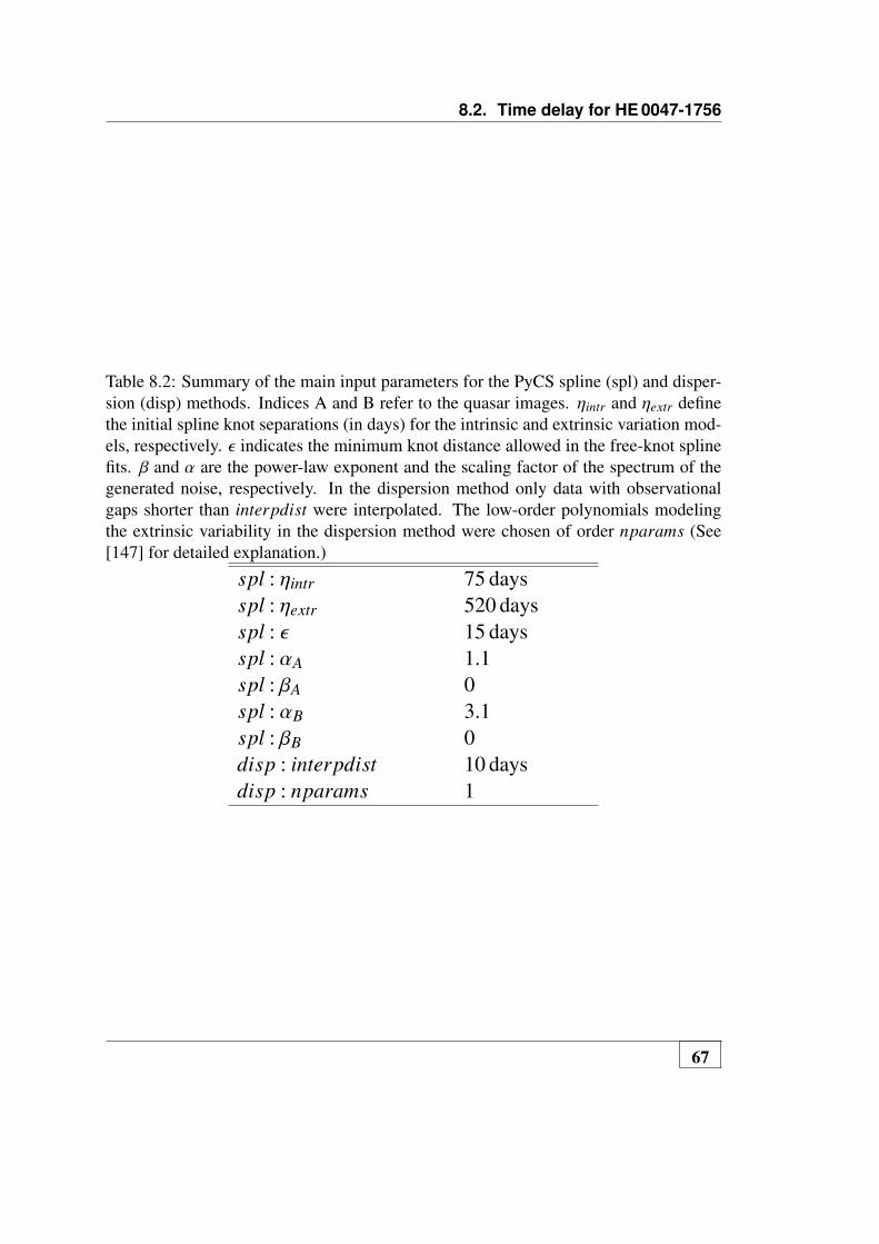
8.2. Time delay for HE 0047-1756
Table 8.2: Summary of the main input parameters for the PyCS spline (spl) and disper-sion (disp) methods. Indices A and B refer to the quasar images. ηintr and ηextr definethe initial spline knot separations (in days) for the intrinsic and extrinsic variation mod-els, respectively. ε indicates the minimum knot distance allowed in the free-knot splinefits. β and α are the power-law exponent and the scaling factor of the spectrum of thegenerated noise, respectively. In the dispersion method only data with observationalgaps shorter than interpdist were interpolated. The low-order polynomials modelingthe extrinsic variability in the dispersion method were chosen of order nparams (See[147] for detailed explanation.)
spl : ηintr 75 daysspl : ηextr 520 daysspl : ε 15 daysspl : αA 1.1spl : βA 0spl : αB 3.1spl : βB 0disp : interpdist 10 daysdisp : nparams 1
67

Chapter 8. HE 0047-1756
least-square fitting figure of merit that takes into account all data points.The dispersion method goes back to the dispersion techniques by [113] and simultane-ously adjusts the time shifts and low-order polynomial representations of the extrinsicvariability in order to minimize a scalar dispersion function that quantifies the devia-tions between the two components of all possible combinations of light curves. Thismethod does not assume any model for the intrinsic variability.The results determined with the spline fitting technique and dispersion technique are7.2± 3.8 days and 8.0± 4.2 days, respectively. The mean value and quoted error barscorrespond to the mean and standard deviation of the resulting time delay distributions,shown in Fig. 8.2 and 8.3, obtained by drawing 1000 realizations of the observed lightcurves. The light curve realizations were drawn taking into account a free-knot splinemodel for the intrinsic variability, a free-knot spline model for extrinsic variability andpower-law noise models for the light curves, as explained in [147]. On the other hand,the application of these methods to the R-band data in the years 2008-2012 failed toconverge to a unique answer.
We carried out a local analysis on year 2008 in the V band in order to confirmthe obtained results and show that the above analysis was not biased by the existenceof the observing gaps. We found out that the best way to analyze such a short lightcurve portion was to follow a linear interpolation scheme, which did not introduce thedifficulties of generating the model for the intrinsic and extrinsic variability – necessaryinputs for the PyCS software in order to draw new realizations of the light curves – froma reduced number of data points. Our approch, aimed at determining the time delaywhich minimizes the magnitude difference between the light curves, was published firstby [54] and goes back to [81]. It proceeded through the following steps:
1. Component A of each of 10000 bootstrap resamplings of the observed light curvewas shifted by the time delay ∆t to be tested. The time delay values were cho-sen in the range from 0 to 50 days (image A leading). Such a high number ofresamplings constrained the uncertainties on the time delay measurement.
2. The light curve of the brightest component A was linearly interpolated in corre-spondence to the dates at which the B light curve had been observed. Only gapsshorter than 20 days were interpolated.
3. Each resampling was smoothed by using a triangular filter with a width δ of 3 and6 days respectively for the brighter component A and the weaker component B.The use of larger windows, i.e. 6 and 12 days, did not change the results. By usinga triangular filter, we determined, for a given component, the magnitude at anyepoch ti as a weighted average of magnitude values corresponding to neighboringepochs t j with |ti− t j| ≤ δ. The triangular weight had the following shape
68

8.2. Time delay for HE 0047-1756
Figure 8.4: Distribution p for time delays between 0−50 days based on our light curvesof components AV and BV . The probability has been computed from 10000 bootstrapresamplings of the observed light curves. For each resampling the brightest componentA has been interpolated in correspondence to the dates at which B has been observed.The region above the dashed line contains 95% of the statistical weight of the distribu-tion, after discarding the peak at 0 lag. Mean value and standard deviation of this regionare ∆t = 7.6±1.8 days.
69
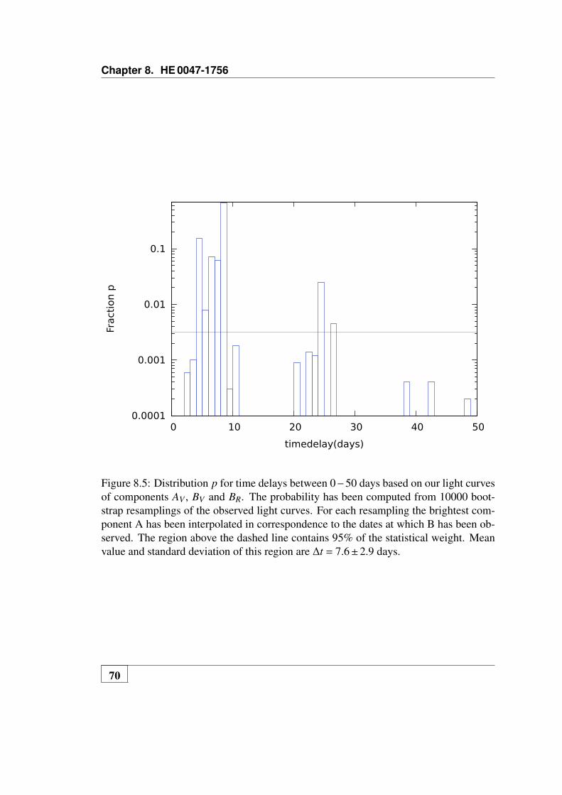
Chapter 8. HE 0047-1756
0.0001
0.001
0.01
0.1
0 10 20 30 40 50
Fract
ion p
timedelay(days)
Figure 8.5: Distribution p for time delays between 0−50 days based on our light curvesof components AV , BV and BR. The probability has been computed from 10000 boot-strap resamplings of the observed light curves. For each resampling the brightest com-ponent A has been interpolated in correspondence to the dates at which B has been ob-served. The region above the dashed line contains 95% of the statistical weight. Meanvalue and standard deviation of this region are ∆t = 7.6±2.9 days.
70

8.2. Time delay for HE 0047-1756
ωi, j =1− |ti−t j|
δ
σ2m j
, (8.1)
where σm j indicates the Poissonian noise corresponding to the magnitude m j ob-served at the epoch t j.
4. From the resulting light curves, comprising N epochs, we computed the weightedmagnitude difference between the components ∆m and determined the χ2
ν
χ2ν =
1N −2
N∑1
(mA(ti)−mB(ti +∆t)−∆m)2
σmA2 +σmB2 , (8.2)
where ti is the generic time at which data has been collected. σmA and σmB arethe Poissonian noise propagated through the interpolation formula for mA(ti) andthe Poissonian noise corresponding to mB(ti +∆t), respectively.
5. The time delay corresponding to the minimum χ2ν was the optimal time delay at
any given resampling (see [54]).
It turned out that only in year 2008 the light curves of components A and B werecharacterized by an intra-seasonal (intrinsic) variation feature useful for the purpose ofdetermining the time delay between the two components. Moreover, the overall A andB light curves did not differ simply by an additional constant, since their differenceincreased as a function of time. By inspection of Fig. 8.1 we noticed that the variationof component AR differed from that of components AV ,BV and BR. The algorithm wasapplied at first to the light curve couple AV BV . The probability distribution of timedelays obtained by using this method is plotted in Fig. 8.4. The probability of each1-day bin was calculated as the ratio between the occurence of light curves with best-fitting time delay in that bin and the total number of resamplings. This procedure alsoincluded a peak at 0-day lag as result, possibly a spurious peak deriving from correlatedbrightness fluctuations at 0 lag. This correlation effect appears when dealing with opticaldiscrete data, as already reported by [154] and by [23], which described it as a frame-to-frame correlation error in the photometry. We computed, for the region above thedashed line, carrying 95% of the statistical weight of the distribution (not taking intoaccount the peak at 0 lag), the mean time delay and the standard deviation, obtaining∆t = 7.6± 1.8 days. In order to assess whether the distribution at 0 lag correspondedto a spurious peak, we applied the above algorithm to the light curve couple AV BVR,where BVR is the average of the light curves of component B in both filters. The aimwas to break the correlation at 0 lag between the multiple photometric data recordedon a single frame (in a given filter). Although it is not strictly clear whether this can
71
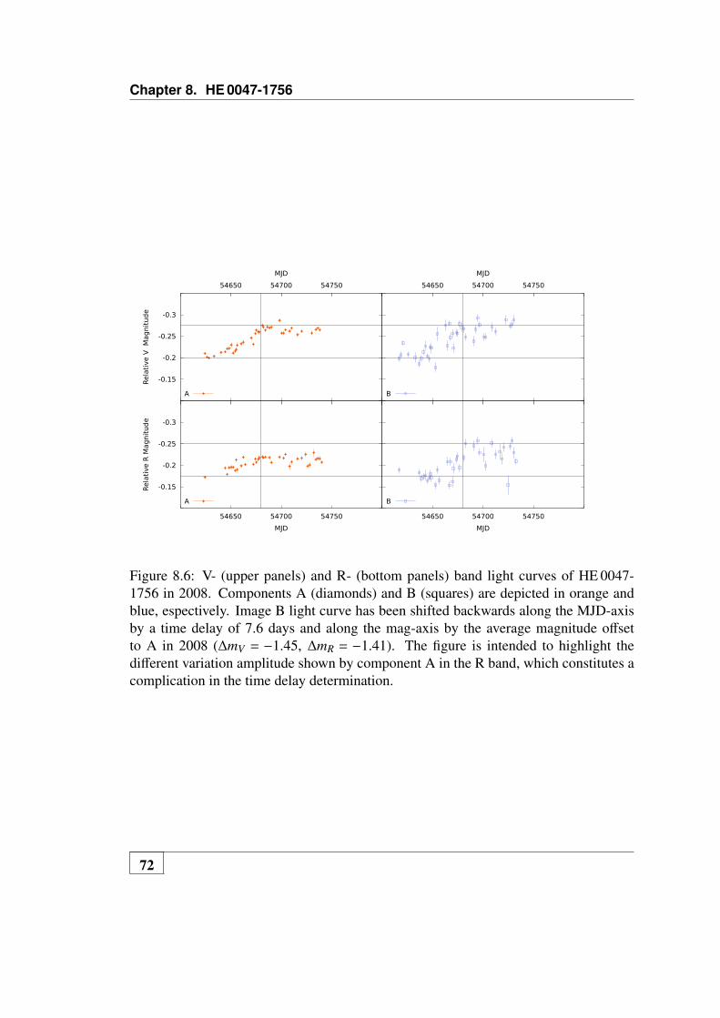
Chapter 8. HE 0047-1756
-0.3
-0.25
-0.2
-0.15
54650 54700 54750
Rela
tive V
M
agnit
ud
e
MJD
A
54650 54700 54750
MJD
B
-0.3
-0.25
-0.2
-0.15
54650 54700 54750
Rela
tive R
Magnit
ud
e
MJD
A
54650 54700 54750
MJD
B
Figure 8.6: V- (upper panels) and R- (bottom panels) band light curves of HE 0047-1756 in 2008. Components A (diamonds) and B (squares) are depicted in orange andblue, espectively. Image B light curve has been shifted backwards along the MJD-axisby a time delay of 7.6 days and along the mag-axis by the average magnitude offsetto A in 2008 (∆mV = −1.45, ∆mR = −1.41). The figure is intended to highlight thedifferent variation amplitude shown by component A in the R band, which constitutes acomplication in the time delay determination.
72
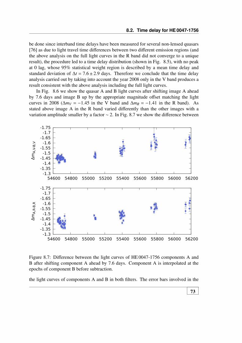
8.2. Time delay for HE 0047-1756
be done since interband time delays have been measured for several non-lensed quasars[76] as due to light travel time differences between two different emission regions (andthe above analysis on the full light curves in the R band did not converge to a uniqueresult), the procedure led to a time delay distribution (shown in Fig. 8.5), with no peakat 0 lag, whose 95% statistical weight region is described by a mean time delay andstandard deviation of ∆t = 7.6± 2.9 days. Therefore we conclude that the time delayanalysis carried out by taking into account the year 2008 only in the V band produces aresult consistent with the above analysis including the full light curves.
In Fig. 8.6 we show the quasar A and B light curves after shifting image A aheadby 7.6 days and image B up by the appropriate magnitude offset matching the lightcurves in 2008 (∆mV = −1.45 in the V band and ∆mR = −1.41 in the R band). Asstated above image A in the R band varied differently than the other images with avariation amplitude smaller by a factor ∼ 2. In Fig. 8.7 we show the difference between
-1.75-1.7
-1.65-1.6
-1.55-1.5
-1.45-1.4
-1.35-1.3
54600 54800 55000 55200 55400 55600 55800 56000 56200
Δm
A,V
-B,V
-1.75-1.7
-1.65-1.6
-1.55-1.5
-1.45-1.4
-1.35-1.3
54600 54800 55000 55200 55400 55600 55800 56000 56200
Δm
A,R
-B,R
Figure 8.7: Difference between the light curves of HE 0047-1756 components A andB after shifting component A ahead by 7.6 days. Component A is interpolated at theepochs of component B before subtraction.
the light curves of components A and B in both filters. The error bars involved in the
73

Chapter 8. HE 0047-1756
difference computation were added in quadrature. From these plots it can be seen asecular evolution of the magnitude difference between the quasar components by ≈ 0.2mag across the 5 periods, which is mainly linear and we explain it as due to a long-termmicrolensing perturbation. Such a behaviour has already been observed for the doublequasar SBS 1520+530 by [54].
-0.25-0.2
-0.15-0.1
-0.05 0
0.05 0.1
0.15 0.2
54600 54800 55000 55200 55400 55600 55800 56000 56200
V-R
Inst
r.
AB
2008 2009 2010 2011 2012
AB
-0.25-0.2
-0.15-0.1
-0.05 0
0.05 0.1
0.15 0.2
54600 54800 55000 55200 55400 55600 55800 56000 56200
ΔV-R
A,B
MJD
Figure 8.8: (V −R)Instr. light curves of HE 0047-1756 from 2008 to 2012. ComponentsA (diamonds) and B (squares) are depicted, respectively, in orange and blue in the firstupper panel. In the bottom panel we show how the color difference between the twocomponents evolves. The difference is computed by interpolating the magnitude of thebrightest component in the pair in correspondence to the dates at which the weakestone has been observed. The horizontal dashed lines define ±0.05 intervals around theaverage color difference.
An analysis of the color index V −RInstr. light curve as a function of the MJD, shownin the upper part of Fig. 8.8, reveals that the two components spanned the highest colorvariation of ≈ 0.07 mag between seasons 2008 and 2009, with both images turning bluer
74

8.2. Time delay for HE 0047-1756
in correspondence to the 2009 brightnening of the quasar, as already observed by [157],[116], [125], [124]. The yearly averages of the color are shown in Table 8.3.
Table 8.3: Yearly averages of the instrumental color V −RInstr. for the two lensed com-ponents of quasar HE 0047-1756.
2008 2009 2010 2011 2012(V −R)Instr.A −0.04±0.02 −0.11±0.01 −0.08±0.02 −0.07±0.01 −0.08±0.01(V −R)Instr.B 0.00±0.03 −0.07±0.04 −0.04±0.05 −0.03±0.05 −0.04±0.04
Table 8.4: Yearly average differences of the instrumental color V −RInstr. between com-ponents A and B of quasar HE 0047-1756.
2008 2009 2010 2011 2012∆(V −R)Instr. −0.04±0.04 −0.03±0.03 −0.05±0.05 −0.04±0.06 −0.03±0.04
The color difference between the quasar images was mainly constant ≈ 0.04 through-out the five seasons, as shown in the bottom panel of Fig. 8.8. We computed the colordifference after shifting the color light curve of component A by 7.6 days and linearlyinterpolating it in correspondence to the observation dates of component B. The errorbars involved in the difference computation were added in quadrature. The yearly av-erages of the color difference are shown in Table 8.4 and are consistent with a constantoffset between the color light curves.
75


9Q 2237+0305
9.1 Light curves for Q 2237+0305
Figures 9.1 and 9.2 show the light curves of the four components of quasar Q 2237+0305in the standard V and R bands. The error bars were determined by using the GALFITsoftware as explained in paragraph 6.4. Figure 9.1 displays the light curves of compo-nents A in fuchsia and pale pink, component B in dark and pale green, component C innavy blue and sky blue, component D in two shades of yellow. The first twelve portionsof the light curves, which are depicted using the lighter colors, represent the results ofthe OGLE campaign from 1997 to 2008, which are available from the OGLE internetarchive 1. We have been able to join up our results with the previous OGLE light curvesin 2008, as explained in section 9.2. The last five years of monitoring, correspondingto our data, are displayed in more intense colors and are labelled at the bottom of theplot. The OGLE monitoring first showed, with smooth well sampled light curves, thatmicrolensing is practically going on all the time in all multiple images of the quasarQ 2237+0305. Since the time delays between the quasar components are predicted tobe of the order of 1 day, the light curves can be straightforwardly compared. None ofthe components followed the same variation pattern, which means that microlensingwas constantly at work during the OGLE monitoring campaign. This is what we alsorecorded during the last five seasons of monitoring. In the V band the flux of imageA became weaker by ≈ 0.5 mag during our monitoring. Image B became dimmer by≈ 0.3 mag. Image C flux turned slowly weaker during the first three season, similarly toimage B, to become then much brighter between 2011 and 2012 by ≈ 0.8 mag. Duringthe five years of monitoring image D became weaker by ≈ 1.25 mag. So all the com-ponents are characterized by more or less dramatic, but independent, variation patterns.The most striking features are seen in image D, which became brighter than image Band C for the first time since the beginning of the OGLE monitoring campaign and thenweaker again, as it used to be in the previous monitoring seasons. Additionally, image Cbecame again weaker than image B after the reported high-magnification event in 1999
1http://ogle.astrouw.edu.pl/
77
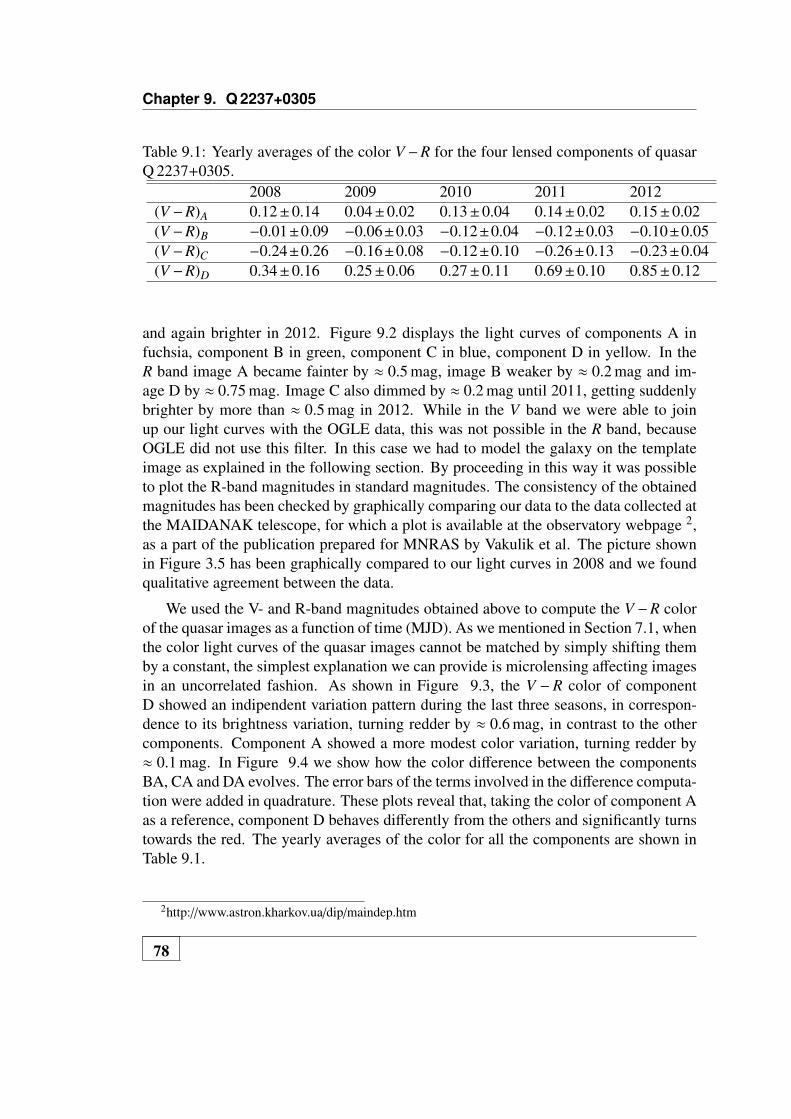
Chapter 9. Q 2237+0305
Table 9.1: Yearly averages of the color V −R for the four lensed components of quasarQ 2237+0305.
2008 2009 2010 2011 2012(V −R)A 0.12±0.14 0.04±0.02 0.13±0.04 0.14±0.02 0.15±0.02(V −R)B −0.01±0.09 −0.06±0.03 −0.12±0.04 −0.12±0.03 −0.10±0.05(V −R)C −0.24±0.26 −0.16±0.08 −0.12±0.10 −0.26±0.13 −0.23±0.04(V −R)D 0.34±0.16 0.25±0.06 0.27±0.11 0.69±0.10 0.85±0.12
and again brighter in 2012. Figure 9.2 displays the light curves of components A infuchsia, component B in green, component C in blue, component D in yellow. In theR band image A became fainter by ≈ 0.5 mag, image B weaker by ≈ 0.2 mag and im-age D by ≈ 0.75 mag. Image C also dimmed by ≈ 0.2 mag until 2011, getting suddenlybrighter by more than ≈ 0.5 mag in 2012. While in the V band we were able to joinup our light curves with the OGLE data, this was not possible in the R band, becauseOGLE did not use this filter. In this case we had to model the galaxy on the templateimage as explained in the following section. By proceeding in this way it was possibleto plot the R-band magnitudes in standard magnitudes. The consistency of the obtainedmagnitudes has been checked by graphically comparing our data to the data collected atthe MAIDANAK telescope, for which a plot is available at the observatory webpage 2,as a part of the publication prepared for MNRAS by Vakulik et al. The picture shownin Figure 3.5 has been graphically compared to our light curves in 2008 and we foundqualitative agreement between the data.
We used the V- and R-band magnitudes obtained above to compute the V −R colorof the quasar images as a function of time (MJD). As we mentioned in Section 7.1, whenthe color light curves of the quasar images cannot be matched by simply shifting themby a constant, the simplest explanation we can provide is microlensing affecting imagesin an uncorrelated fashion. As shown in Figure 9.3, the V − R color of componentD showed an indipendent variation pattern during the last three seasons, in correspon-dence to its brightness variation, turning redder by ≈ 0.6 mag, in contrast to the othercomponents. Component A showed a more modest color variation, turning redder by≈ 0.1 mag. In Figure 9.4 we show how the color difference between the componentsBA, CA and DA evolves. The error bars of the terms involved in the difference computa-tion were added in quadrature. These plots reveal that, taking the color of component Aas a reference, component D behaves differently from the others and significantly turnstowards the red. The yearly averages of the color for all the components are shown inTable 9.1.
2http://www.astron.kharkov.ua/dip/maindep.htm
78

9.1. Light curves for Q 2237+0305
15.5
16
16.5
17
17.5
18
18.5
19
19.5 50000 51000 52000 53000 54000 55000 56000 57000
V
MJD
star-2
A
B
C
D
2008 2009 2010 2011 2012
Figure 9.1: V-band light curves of Q 2237+0305 from 2008 to 2012 are shown on theright side of the plot. Components A (filled dots), B (asterisks), C (squares), D (filleddiamonds) are depicted in fuchsia, green, blue and yellow, respectively. The light curveof a star in the field, labelled as Const. in Fig. 4.6, is shown in black and shifted by−2 mag. The light curves from the MiNDSTEp campaign have been photometricallyjoined up with the 12-year-long OGLE data.
79

Chapter 9. Q 2237+0305
Figure 9.2: R-band light curves of Q 2237+0305 from 2008 to 2012. Components A(filled dots), B (asterisks), C (squares), D (filled diamonds) are depicted in fuchsia,green, blue and yellow, respectively. The light curve of component D is shifted by+0.5 mag. The light curve of a star in the field, labelled as Const. in Fig. 4.6, is shownin black and shifted by −1.5 mag.
80

9.1. Light curves for Q 2237+0305
-1
-0.8
-0.6
-0.4
-0.2
0
0.2
0.4
0.6
0.8
1
1.2
54600 54800 55000 55200 55400 55600 55800 56000 56200
V-R
MJD
A
B
C
D
2008 2009 2010 2011 2012
Figure 9.3: V −R color of the components of the quasar Q 2237+0305 as a function ofthe MJD. Components A (filled dots), B (asterisks), C (squares), D (filled diamonds)are depicted in fuchsia, green, blue and yellow, respectively. The years in which datawere collected appear at the bottom of the figure.
81

Chapter 9. Q 2237+0305
-1
-0.5
0
0.5
54600 54800 55000 55200 55400 55600 55800 56000 56200
ΔV-R
B,A
-1
-0.5
0
0.5
54600 54800 55000 55200 55400 55600 55800 56000 56200
ΔV-R
C,A
-1
-0.5
0
0.5
54600 54800 55000 55200 55400 55600 55800 56000 56200
ΔV-R
D,A
MJD
Figure 9.4: Differences of the V −R colors of the component pairs BA, CA and DA ofthe quasar Q 2237+0305 as a function of the time (MJD).
82

9.2. Q 2237+0305 standard photometry: modeling the galaxy on the R-bandtemplate
9.2 Q 2237+0305 standard photometry: modeling thegalaxy on the R-band template
The measurement of the flux for the template image FX,T , which is necessary tocalculate the magnitude as in equation 7.1, was calculated by neglecting the presenceof the weak lensing galaxies in the case of WFI 2033-4723 and HE 0047-1756. Thiswas no longer possible in the case of Q 2237+0305, whose lens is a barred spiral galaxywith an average magnitude of ≈ 15 mag in the optical bands ([177], [135], [127]). In theV band, our approach consisted in avoiding the galaxy modeling. Since in our imagesthe galaxy is not well resolved, an attempt to fit a model to the galaxy has generally beenregarded as the last resort. The OGLE light curves in the V band are public and theirstandard photometry was obtained by modeling the galaxy on HST images of the lens,as explained in [173]. Therefore, we opted for simply joining our light curves to theOGLE light curves. This was possible by noticing that, at any given night, the unknownflux of image i on the template is related to the corresponding image magnitude mAi,measured by OGLE, by the following relation
Ai +δAi = Aα10mα−mAi
2.5 (9.1)
where Ai + δAi is the sum of the flux on the template and the differential flux com-puted at that night, Aα the number of counts per second of the α star showed in Fig. 4.6,and mα its magnitude, fixed at 17.5 mag according to [173]. We chose a good seeingnight, common to our data and the OGLE campaign, and corresponding to a Modi-fied Julian Date (MJD) of 54685.3 days. Substituting the values corresponding to eachquasar image in the previous formula, we obtained, for each of them, the number ofcounts per second Ai for the template image. This allowed to translate our differentialfluxes into total magnitudes, as those used for the OGLE light curves. The magnitudeof the star α, mα, and its flux at the chosen night provided the zero point needed to jointhe data.On the other hand, in the R band, we could not compare our data with any other pub-lished light curves. So we chose to model the lensing galaxy of the quasar Q 2237+0305by using the GALFIT software. The model consisted of:
1. The four point-like images of the quasar. The system geometry was fixed asoutlined in Table 6.1. The position of one image was allowed to vary togetherwith the fluxes of the four images.
2. A galactic exponential disk profile component.
3. A de Vaucouleurs’ profile for the galactic bulge.
These choices are based on the evidence that a disk galaxy is a composite system welldescribed by a combination of an exponential disk and a de Vaucouleurs’ bulge profile.
83

Chapter 9. Q 2237+0305
A de Vaucouleurs’ profile contributes to describing the surface brightness of an ellipticalgalaxy and can be written as a function B(r) of the distance r from the center, as follows
B(r) = Iee−7.67[( rRe )1/4−1] (9.2)
where Ie is the surface brightness at the radius Re, which encloses the disk region con-tributing to half of the galaxy brightness. This is a special case of Sersic’s law, where theSersic’s index is fixed at n=4. The exponential disk component I(r) typically describesthe profile of disk galaxies at large radii and has the shape
I(r) = Ioe(− rRo ) (9.3)
where Io represents the surface brightness of this component at the center of the diskand Ro is the exponential scale length.
For both the exponential disk and the de Vaucouleurs’ profile components, the inputparameters were the disk ellipticity, measured on the image and fixed at 0.65, and thePA, the position angle describing the orientation of the disk major axis, fixed at 58.36degrees towards the right, as seen in Figure 4.6. Both the parameters were measured byusing simple graphic tools of the package ds9. For both profiles the central position wasleft free, together with the profile scales Re and Ro and the total profile magnitudes. Theresult of the fit is summarized in Table 9.2.
By adding the fluxes on the template image to the differential fluxes computed foreach night and by making use of the standard magnitude for the star α in the R band(Ralpha = 17.28 mag according to [25]), it was possible to plot the light curves in stan-dard magnitudes. The best fit model that we used is far from being accurate, since thelensing galaxy in Q 2237+0305 shows an important bar component that cannot easilybe modeled with simple galaxy model profiles. Nevertheless in quasar microlensing therelative flux variations between the quasar components are the prime focus of interestand obtaining the light curves in standard magnitudes does not add any fundamentaldetail to our knowledge of microlensing, and can be regarded as a refining exercise.
84

9.2. Q 2237+0305 standard photometry: modeling the galaxy on the R-bandtemplate
Table 9.2: The table summarizes the best fit model parameters for the lensing galaxy ofthe system Q 2237+0305 in the R band. The labels xindex, yindex represent the centralposition of the brightness profiles. The letters A, B, C ,D stand for the flux of the quasarcomponents on the R-band template image, Mindex indicates the integrated instrumentalmagnitudes of the brightness profiles.
xA 777.4 pxyA 679.3 pxA 1477 counts/sB 450 counts/sC 278 counts/sD 641 counts/sxdeVac 776 pxydeVac 681 pxMdeVac 16.4 magRe 4.7 pxxexp 776 pxyexp 682 pxMexp 15.5 magRo 10.4 pxχ2 42
85

10Summary and conclusions
10.1 Summary
We have presented V-band and R-band photometry of the gravitational lens systemsWFI 2033-4723, HE 0047-1756 and Q 2237+0305 from 2008 to 2012. Data were col-lected by the MiNDSTEp collaboration with the Danish 1.54 m telescope at La Silla,Chile. By applying the Alard & Lupton image subtraction method ([9], [8]), as imple-mented in the HOTPAnTS software, we have constructed the light curves of the multipleimages of the quasars.
1. The lensed images of the quasar WFI 2033-4723 varied by ≈ 0.6 mag in the Vband and ≈ 0.5 mag in the R band during the campaign, becoming brighter in2009 and gradually weaker until 2012. After computing the A2-A1, B-A1, C-A1 light curves, we found that C-A1 showed a variation of ≈ 0.2 mag in the Rband across the period 2008-2011. We suggest that microlensing affecting onlythe outer part of the accretion disk of image C could in principle explain the be-haviour seen in the R band. This relies on the hypothesis that an outer and hencecooler part of the disk, with emission at longer wavelengths, is magnified by thecaustic pattern.
2. The two lensed components of quasar HE 0047-1756 reached their maximumbrightness in 2009 and again in 2012, with a magnitude variation of ≈ 0.2 −0.3 mag. We were able to provide a measurement of the time delay between thetwo components of this system for the first time. We applied the PyCS softwareby [147] to our whole V-band and R-band dataset. The free-knot spline techniqueand dispersion technique provided in the V-band consistent estimates of the timedelay of 7.2±3.8 and 8.0±4.2 days. In the R-band the methods did not convergeto a unique result. By making use of a linear-interpolation scheme applied to thebrightest component A (see [54]), we carried out a zoom-in analysis on 2008 anddetermined the time delay value minimizing the magnitude difference between
87

Chapter 10. Summary and conclusions
the light curves AV and BV . We found out that component B is delayed with re-spect to A by ∆t = 7.6±1.8 days. In order to verify the spurious nature of a 0 lagpeak, included as a possible result in the above zoom-in analysis, we applied thelinear-interpolation scheme to the light curves AV and BVR. The latter is the aver-age of the light curves BV and BR in 2008. We estimated the corresponding timedelay at ∆t = 7.6±2.9 days. Therefore, we conclude that the time delay analysiscarried out by taking into account only the year 2008 in the V band produces aresult consistent with the analysis including the full light curves. The magnitudedifference between the light curves of A and B in both bands increased from 2008to 2012 by ≈ 0.2 mag, showing a long-term linear uncorrelation between the twocomponents, which can be explained with a long-term microlensing perturbation.The images of quasars WFI 2033-4723 and HE 0047-1756 became bluer whengetting brighter. This is consistent with previous studies (e.g. [157]). A possibleexplanation to this finding is obtained by considering the accretion disk modelsfor quasars. A boost in the disk accretion rate could produce a temperature in-crease of the inner regions of a quasar, hence a brighter and bluer emission. Thecolor difference between the components of each quasar is consistent with beingconstant across the five periods.
3. In the case of quasar Q 2237+0305 we were able to compute the photometry instandard magnitudes, joining up our curves with the OGLE ones in the V bandand recurring to modeling the lensing galaxy in the R band. As already demon-strated by the previous monitoring campaigns, all the components of the systemshowed impressive and uncorrelated variations of flux. In the V band, image Abecame fainter by ≈ 0.5 mag during the 5-year monitoring. Image B became in-stead dimmer by ≈ 0.3 mag. Image C flux turned slowly dimmer during the firstthree season, similarly to image B, to become then much brighter between 2011and 2012 by ≈ 0.8 mag. Image D dimmed by ≈ 1.25 mag. Hence, all the compo-nents showed independent variation patterns. The most striking features are seenin image D, which became brighter than image B and C for the first time sincethe beginning of the OGLE monitoring and then weaker again, in what appears tobe a typical shape of a high-magnification event. Image C became again weakerthan image B after the reported high-magnification event in 1999 (MJD ≈ 51400)and brighter in 2012, in what resembles the ascending portion of another high-magnification event. We found similar variation patterns in the R band. ImageA became fainter by ≈ 0.5 mag, image B by ≈ 0.2 mag, image D by ≈ 0.75 magand image C by ≈ 0.2 mag until 2011, getting suddenly brighter by more than≈ 0.5 mag in 2012. The computation of the V −R colors of the quasar compo-nents indicated that component D became redder by ≈ 0.6 mag, in contrast to thesmaller color variations of the other components. Chromatic microlensing mightprovide an explanation to this finding.
88

10.2. Conclusions and outlook
10.2 Conclusions and outlook
This thesis work has focussed on the observation of the quasar microlensing phe-nomenon in multiply imaged quasars. The relative light curves have been built bymaking use of the difference image analysis (DIA), arguably the best way of treatingvariable sources in presence of wide overlapping and non-varying galaxies. The out-standing results obtained with a 1.5 m class telescope, average exposures of 3 minutesand an average seeing of 1.3 ′′, reveals how the technique has a huge potential for in-vestigating an increased number of gravitational systems, with the aim of computingtime delays and accessing the spatial structure of distant quasars. The possible devel-opment of a more automated software would help meet the requirement of analyzing alarger number of systems in order to build wider statistical samples, from which deduc-ing fundamental astrophysical quantities and scales. Since 2012, no additional quasarmonitoring has been going on at the Danish telescope. Nevertheless, a new quasar mon-itoring campaign has been started at the Las Cumbres Observatory Global TelescopeNetwork (LCOGT) and the method presented above has already been applied to thefirst data.
89


11Appendix A
Photometry of WFI 2033-4723, HE 0047-1756 and Q 2237+0305.
91

Chapter 11. Appendix A
Tabl
e11
.1:V
-and
R-b
and
phot
omet
ryof
HE
0047
-175
6,a
sin
Fig.
8.1.
mag
AV
σA,V
mag
BV
σB,V
mag
AR
σA,R
mag
BR
σB,R
MJD
-0.2
10.
003
1.25
10.
007
-0.1
720.
003
1.22
40.
007
5462
4.4
-0.2
020.
003
1.24
30.
008
5462
6.4
-0.2
0.00
21.
216
0.00
554
628.
4-0
.204
0.00
21.
241
0.00
654
633.
4-0
.213
0.00
41.
249
0.01
154
640.
4-0
.214
0.00
41.
264
0.00
9-0
.194
0.00
41.
229
0.00
954
644.
4-0
.221
0.00
31.
251
0.00
8-0
.179
0.00
41.
244
0.00
854
646.
4-0
.222
0.00
31.
237
0.00
7-0
.195
0.00
31.
239
0.00
754
648.
4-0
.23
0.00
51.
222
0.01
2-0
.196
0.00
51.
236
0.01
254
650.
4-0
.211
0.00
21.
245
0.00
5-0
.195
0.00
21.
249
0.00
654
652.
4-0
.216
0.00
31.
252
0.00
8-0
.188
0.00
21.
243
0.00
654
654.
4-0
.22
0.00
31.
225
0.00
6-0
.213
0.00
41.
233
0.00
954
655.
4-0
.229
0.00
51.
227
0.01
2-0
.19
0.00
41.
241
0.01
5465
6.4
-0.2
330.
004
1.27
20.
011
-0.1
990.
004
1.25
90.
009
5466
0.3
-0.2
360.
006
1.19
40.
015
-0.2
190.
004
1.22
40.
009
5466
2.3
-0.2
020.
004
1.24
80.
009
5466
4.3
-0.2
460.
005
1.17
40.
013
5467
0.3
-0.2
320.
005
1.22
10.
011
-0.2
030.
004
1.20
40.
009
5467
2.3
-0.2
560.
003
1.17
0.00
7-0
.215
0.00
41.
259
0.00
954
674.
3-0
.264
0.00
31.
203
0.00
8-0
.207
0.00
41.
204
0.00
854
675.
3-0
.26
0.00
41.
193
0.00
8-0
.214
0.00
61.
251
0.01
354
677.
3-0
.26
0.00
41.
227
0.01
-0.2
180.
005
1.22
0.01
254
678.
3-0
.275
0.00
41.
190.
009
-0.2
20.
004
1.19
90.
009
5468
1.3
-0.2
710.
004
1.19
20.
009
-0.2
180.
003
1.19
20.
008
5468
2.3
-0.2
640.
003
1.17
0.00
7-0
.219
0.00
41.
219
0.00
954
684.
3-0
.272
0.00
51.
179
0.01
154
686.
3-0
.27
0.00
31.
183
0.00
8-0
.218
0.00
41.
195
0.00
854
688.
3-0
.272
0.00
31.
201
0.00
8-0
.207
0.00
51.
162
0.01
154
690.
3-0
.287
0.00
41.
211
0.01
1-0
.219
0.00
51.
168
0.01
254
698.
3-0
.257
0.00
41.
183
0.00
954
700.
3-0
.257
0.00
41.
157
0.00
9-0
.217
0.00
41.
156
0.00
954
702.
4-0
.265
0.00
31.
173
0.00
7-0
.226
0.00
31.
183
0.00
854
704.
2-0
.262
0.00
41.
202
0.00
8-0
.198
0.00
81.
188
0.01
754
708.
2-0
.269
0.00
31.
201
0.00
8-0
.208
0.00
51.
214
0.01
154
710.
2-0
.254
0.00
41.
178
0.01
-0.2
150.
004
1.16
10.
009
5471
6.2
-0.2
620.
003
1.18
90.
009
-0.2
170.
005
1.18
70.
011
5472
0.3
-0.2
260.
007
1.18
10.
0254
724.
2-0
.198
0.00
51.
198
0.01
354
726.
2-0
.201
0.00
41.
170.
0154
728.
2-0
.257
0.00
51.
162
0.01
154
730.
3-0
.23
0.01
1.25
80.
022
5473
2.3
-0.2
660.
003
1.17
60.
008
-0.2
140.
004
1.16
90.
009
5473
4.3
-0.2
690.
004
1.17
20.
008
-0.2
160.
003
1.15
50.
007
5473
6.3
-0.2
650.
004
1.16
10.
01-0
.215
0.00
51.
183
0.01
354
738.
2-0
.207
0.00
41.
203
0.00
854
740.
2-0
.344
0.00
31.
092
0.00
655
066.
4-0
.455
0.00
51.
030.
011
-0.3
70.
005
1.04
50.
011
5506
7.4
-0.4
960.
006
1.05
30.
015
-0.3
670.
005
1.06
90.
011
5506
8.3
92
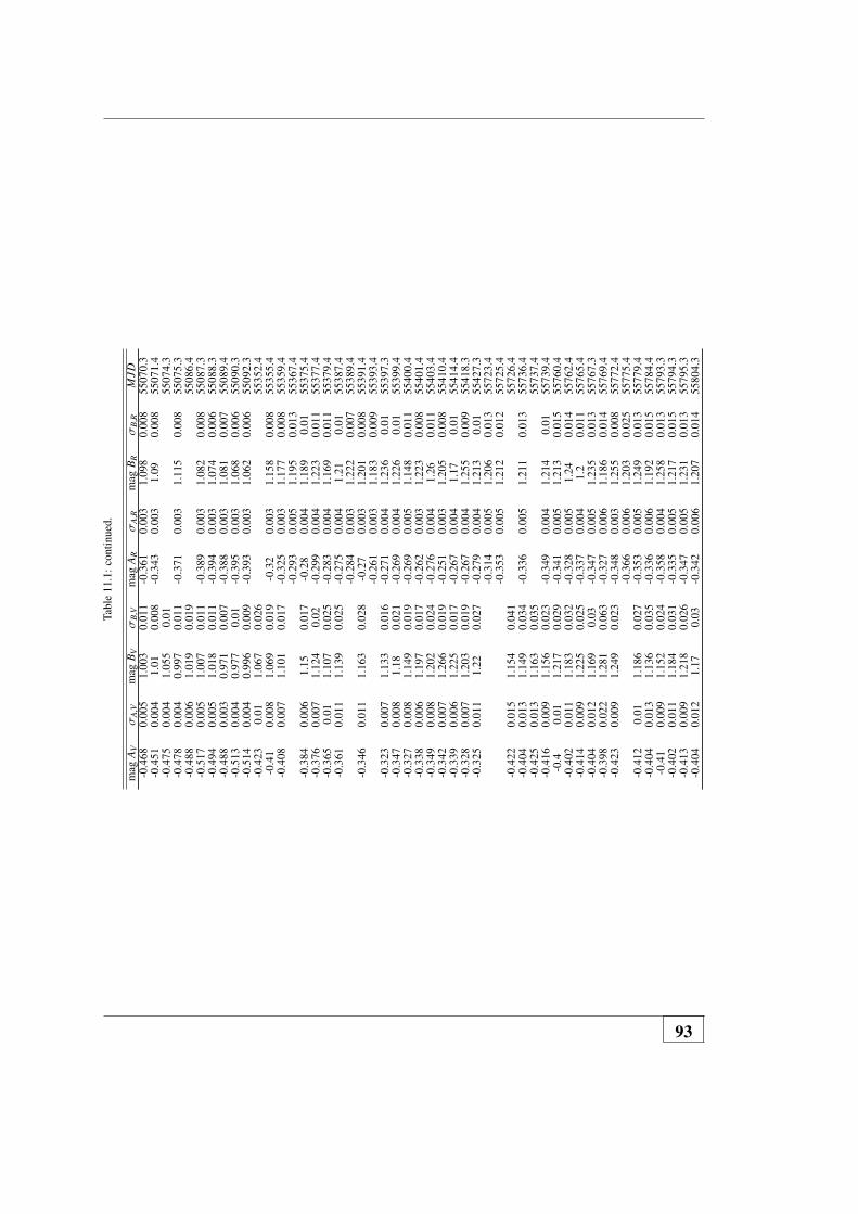
Tabl
e11
.1:c
ontin
ued.
mag
AV
σA,V
mag
BV
σB,V
mag
AR
σA,R
mag
BR
σB,R
MJD
-0.4
680.
005
1.00
30.
011
-0.3
610.
003
1.09
80.
008
5507
0.3
-0.4
510.
004
1.01
0.00
8-0
.343
0.00
31.
090.
008
5507
1.4
-0.4
750.
004
1.05
50.
0155
074.
3-0
.478
0.00
40.
997
0.01
1-0
.371
0.00
31.
115
0.00
855
075.
3-0
.488
0.00
61.
019
0.01
955
086.
4-0
.517
0.00
51.
007
0.01
1-0
.389
0.00
31.
082
0.00
855
087.
3-0
.494
0.00
51.
018
0.01
1-0
.394
0.00
31.
074
0.00
655
088.
3-0
.488
0.00
30.
971
0.00
7-0
.388
0.00
31.
081
0.00
755
089.
4-0
.513
0.00
40.
977
0.01
-0.3
950.
003
1.06
80.
006
5509
0.3
-0.5
140.
004
0.99
60.
009
-0.3
930.
003
1.06
20.
006
5509
2.3
-0.4
230.
011.
067
0.02
655
352.
4-0
.41
0.00
81.
069
0.01
9-0
.32
0.00
31.
158
0.00
855
355.
4-0
.408
0.00
71.
101
0.01
7-0
.325
0.00
31.
177
0.00
855
359.
4-0
.293
0.00
51.
195
0.01
355
367.
4-0
.384
0.00
61.
150.
017
-0.2
80.
004
1.18
90.
0155
375.
4-0
.376
0.00
71.
124
0.02
-0.2
990.
004
1.22
30.
011
5537
7.4
-0.3
650.
011.
107
0.02
5-0
.283
0.00
41.
169
0.01
155
379.
4-0
.361
0.01
11.
139
0.02
5-0
.275
0.00
41.
210.
0155
387.
4-0
.284
0.00
31.
222
0.00
755
389.
4-0
.346
0.01
11.
163
0.02
8-0
.27
0.00
31.
201
0.00
855
391.
4-0
.261
0.00
31.
183
0.00
955
393.
4-0
.323
0.00
71.
133
0.01
6-0
.271
0.00
41.
236
0.01
5539
7.3
-0.3
470.
008
1.18
0.02
1-0
.269
0.00
41.
226
0.01
5539
9.4
-0.3
270.
008
1.14
90.
019
-0.2
690.
005
1.14
80.
011
5540
0.4
-0.3
380.
006
1.19
70.
017
-0.2
620.
003
1.22
30.
008
5540
1.4
-0.3
490.
008
1.20
20.
024
-0.2
760.
004
1.26
0.01
155
403.
4-0
.342
0.00
71.
266
0.01
9-0
.251
0.00
31.
205
0.00
855
410.
4-0
.339
0.00
61.
225
0.01
7-0
.267
0.00
41.
170.
0155
414.
4-0
.328
0.00
71.
203
0.01
9-0
.267
0.00
41.
255
0.00
955
418.
3-0
.325
0.01
11.
220.
027
-0.2
790.
004
1.21
30.
0155
427.
3-0
.314
0.00
51.
206
0.01
355
723.
4-0
.353
0.00
51.
212
0.01
255
725.
4-0
.422
0.01
51.
154
0.04
155
726.
4-0
.404
0.01
31.
149
0.03
4-0
.336
0.00
51.
211
0.01
355
736.
4-0
.425
0.01
31.
163
0.03
555
737.
4-0
.416
0.00
91.
156
0.02
3-0
.349
0.00
41.
214
0.01
5573
9.4
-0.4
0.01
1.21
70.
029
-0.3
410.
005
1.21
30.
015
5576
0.4
-0.4
020.
011
1.18
30.
032
-0.3
280.
005
1.24
0.01
455
762.
4-0
.414
0.00
91.
225
0.02
5-0
.337
0.00
41.
20.
011
5576
5.4
-0.4
040.
012
1.16
90.
03-0
.347
0.00
51.
235
0.01
355
767.
3-0
.398
0.02
21.
281
0.06
3-0
.327
0.00
61.
186
0.01
455
769.
4-0
.423
0.00
91.
249
0.02
3-0
.348
0.00
31.
255
0.00
855
772.
4-0
.366
0.00
61.
203
0.02
555
775.
4-0
.412
0.01
1.18
60.
027
-0.3
530.
005
1.24
90.
013
5577
9.4
-0.4
040.
013
1.13
60.
035
-0.3
360.
006
1.19
20.
015
5578
4.4
-0.4
10.
009
1.15
20.
024
-0.3
580.
004
1.25
80.
013
5579
3.3
-0.4
020.
011
1.18
40.
031
-0.3
350.
005
1.21
70.
015
5579
4.3
-0.4
130.
009
1.21
80.
026
-0.3
470.
005
1.23
10.
013
5579
5.3
-0.4
040.
012
1.17
0.03
-0.3
420.
006
1.20
70.
014
5580
4.3
93

Chapter 11. Appendix A
Tabl
e11
.1:c
ontin
ued.
mag
AV
σA,V
mag
BV
σB,V
mag
AR
σA,R
mag
BR
σB,R
MJD
-0.5
010.
011
1.08
80.
029
-0.4
050.
012
1.10
70.
029
5612
4.9
-0.5
130.
014
1.09
90.
037
-0.4
160.
011.
109
0.02
556
127.
9-0
.523
0.00
81.
070.
026
-0.4
480.
005
1.17
80.
015
5613
4.8
-0.5
250.
012
1.06
90.
032
-0.4
50.
009
1.10
80.
022
5613
5.9
-0.5
450.
011.
082
0.03
-0.4
540.
007
1.15
40.
021
5613
9.9
-0.5
330.
011
1.02
10.
029
5616
4.8
-0.5
410.
011.
033
0.02
7-0
.467
0.00
91.
096
0.02
156
167.
9-0
.532
0.00
81.
117
0.02
1-0
.454
0.00
61.
142
0.01
756
179.
8-0
.53
0.01
21.
096
0.03
1-0
.435
0.01
21.
089
0.02
856
181.
7-0
.535
0.01
1.11
0.02
9-0
.462
0.00
91.
175
0.02
556
186.
7
94

Tabl
e11
.2:V
-and
R-b
and
phot
omet
ryof
WFI
2033
-472
3,a
sin
Fig.
7.1.
mag
BV
σB,V
mag
A1 V
σA
1,V
mag
A2 V
σA
2,V
mag
CV
σC,V
mag
BR
σB,R
mag
A1 R
σA
1,R
mag
A2 R
σA
2,R
mag
CR
σC,R
MJD
2.00
30.
006
1.43
0.00
72.
015
0.01
12.
310.
009
2.07
30.
007
1.45
60.
008
2.01
0.01
32.
296
0.00
954
623.
41.
979
0.00
41.
461
0.00
61.
985
0.00
82.
273
0.00
52.
056
0.00
21.
473
0.00
21.
990.
002
2.28
60.
002
5462
5.4
1.98
80.
004
1.45
60.
006
2.00
60.
009
2.30
60.
007
2.06
40.
002
1.45
90.
002
1.99
70.
003
2.29
10.
002
5462
7.4
1.99
40.
006
1.44
40.
007
2.03
90.
012.
295
0.00
82.
056
0.00
41.
454
0.00
32.
008
0.00
52.
293
0.00
454
629.
42.
026
0.01
1.45
40.
016
2.00
30.
025
2.30
50.
015
2.05
60.
007
1.48
0.00
81.
988
0.01
22.
267
0.01
5464
1.4
2.02
10.
008
1.39
70.
009
2.04
80.
013
2.31
90.
009
2.08
80.
004
1.44
30.
004
2.03
90.
005
2.29
80.
004
5464
5.4
2.04
70.
005
1.43
90.
006
2.02
50.
008
2.35
40.
006
2.08
50.
004
1.46
0.00
31.
998
0.00
52.
304
0.00
354
647.
42.
051
0.00
71.
431
0.00
82.
029
0.01
32.
363
0.00
92.
093
0.00
61.
461
0.00
72
0.01
22.
290.
008
5464
9.4
2.06
0.00
71.
385
0.00
92.
046
0.01
42.
385
0.01
2.08
50.
005
1.43
60.
006
2.03
0.00
92.
310.
006
5465
1.4
2.02
10.
017
1.47
30.
031.
990.
046
2.38
70.
029
5465
3.4
2.07
10.
008
1.39
60.
009
2.05
0.01
32.
359
0.01
2.09
20.
004
1.45
90.
003
1.99
60.
004
2.31
30.
004
5465
5.4
2.03
70.
011
1.49
0.01
51.
910.
022
2.36
60.
016
2.11
70.
011
1.47
30.
014
1.97
60.
021
2.31
60.
015
5465
7.4
2.05
10.
009
1.42
10.
009
2.02
20.
013
2.35
60.
012
2.12
30.
009
1.45
30.
008
2.00
10.
011
2.29
20.
0154
661.
32.
038
0.00
91.
426
0.01
32.
062
0.02
22.
337
0.01
32.
106
0.00
91.
457
0.01
42.
028
0.02
22.
328
0.01
354
671.
32.
040.
009
1.40
40.
012.
123
0.01
82.
390.
012
2.08
40.
011
1.44
90.
013
2.04
60.
021
2.31
90.
015
5467
4.3
2.04
30.
007
1.44
10.
009
2.07
50.
013
2.34
40.
009
2.07
80.
007
1.46
40.
008
2.04
70.
012
2.29
60.
008
5467
5.3
2.04
10.
006
1.48
20.
007
2.02
10.
012.
360.
008
2.08
30.
006
1.49
30.
007
2.03
40.
009
2.30
30.
006
5467
7.3
1.96
20.
022
1.46
90.
038
2.07
60.
066
2.37
0.03
854
679.
32.
014
0.01
41.
432
0.01
52.
057
0.02
22.
339
0.01
92.
070.
006
1.5
0.00
71.
988
0.00
92.
30.
007
5468
1.3
2.01
10.
008
1.53
30.
012.
007
0.01
42.
284
0.00
92.
082
0.00
61.
535
0.00
81.
986
0.01
2.27
90.
008
5468
3.3
2.00
80.
006
1.52
90.
008
2.02
30.
011
2.32
70.
007
2.07
90.
006
1.52
30.
007
2.02
20.
012.
290.
008
5468
5.3
2.01
30.
004
1.51
90.
007
2.04
30.
012.
364
0.00
82.
043
0.01
11.
499
0.01
12.
099
0.01
72.
293
0.01
354
687.
31.
995
0.00
91.
533
0.01
12.
028
0.01
52.
350.
013
2.05
90.
009
1.49
0.01
2.03
30.
015
2.31
0.01
254
699.
32.
012
0.01
1.51
90.
013
2.03
0.01
92.
427
0.01
42.
069
0.00
81.
515
0.01
2.03
10.
016
2.28
80.
011
5470
3.3
2.04
30.
008
1.55
20.
011
1.97
50.
015
2.34
10.
011
2.06
90.
008
1.49
50.
012.
027
0.01
52.
315
0.01
154
705.
31.
999
0.01
11.
501
0.01
81.
998
0.02
82.
378
0.01
82.
070.
012
1.52
90.
016
1.96
50.
023
2.32
60.
016
5471
5.2
1.99
70.
008
1.46
20.
012.
024
0.01
42.
334
0.01
12.
056
0.00
91.
514
0.01
1.97
50.
013
2.33
90.
011
5471
7.2
1.98
50.
012
1.47
30.
013
1.99
20.
022.
379
0.01
72.
086
0.00
91.
460.
012.
069
0.01
62.
353
0.01
354
728.
22.
044
0.01
41.
519
0.02
21.
942
0.03
2.39
30.
024
2.07
50.
011
1.52
50.
015
1.94
90.
021
2.26
30.
016
5472
9.2
2.01
20.
006
1.47
0.00
62.
003
0.00
82.
363
0.00
82.
062
0.00
51.
488
0.00
62
0.00
82.
316
0.00
654
731.
22.
025
0.00
51.
461
0.00
72.
048
0.01
12.
391
0.00
82.
054
0.00
51.
489
0.00
72.
003
0.01
2.33
30.
007
5473
3.2
2.02
40.
012
1.49
80.
017
20.
026
2.37
60.
018
2.05
70.
015
1.49
10.
023
2.06
10.
038
2.28
90.
022
5473
5.1
2.02
50.
009
1.52
80.
011
2.00
20.
016
2.33
80.
011
2.08
10.
008
1.52
30.
012
2.01
20.
017
2.30
90.
014
5473
9.1
2.02
0.00
61.
481
0.00
82.
036
0.01
22.
365
0.00
82.
048
0.00
61.
479
0.00
72.
045
0.00
92.
332
0.00
754
741.
12.
025
0.00
61.
507
0.00
92.
022
0.01
22.
353
0.00
92.
055
0.00
71.
522
0.00
92.
028
0.01
22.
293
0.00
854
743.
11.
808
0.01
1.30
10.
016
1.77
10.
024
2.14
90.
017
5500
1.4
1.81
10.
006
1.29
60.
011
1.87
20.
018
2.19
0.01
255
004.
41.
816
0.00
71.
332
0.01
21.
807
0.01
82.
188
0.01
355
005.
41.
820.
008
1.32
60.
012
1.82
0.01
82.
168
0.01
355
006.
41.
810.
007
1.30
30.
011
1.81
10.
017
2.20
60.
012
5500
8.4
1.63
60.
006
1.11
20.
006
1.71
80.
008
2.11
40.
008
1.73
90.
005
1.16
80.
006
1.74
60.
008
2.10
80.
007
5506
8.2
1.61
10.
007
1.10
10.
006
1.70
30.
008
2.10
60.
009
1.72
0.00
51.
175
0.00
61.
722
0.00
72.
123
0.00
755
070.
21.
623
0.00
51.
112
0.00
61.
693
0.00
82.
101
0.00
71.
743
0.00
51.
203
0.00
61.
672
0.00
72.
129
0.00
655
071.
21.
609
0.00
61.
099
0.00
61.
712
0.00
92.
079
0.00
71.
699
0.00
61.
201
0.00
61.
675
0.00
82.
117
0.00
655
072.
21.
734
0.01
31.
169
0.02
1.70
90.
032
2.17
50.
027
5507
5.2
1.72
40.
018
1.11
10.
026
1.76
0.04
52.
248
0.03
855
076.
21.
629
0.00
71.
070.
008
1.66
70.
013
2.12
40.
009
1.73
70.
007
1.11
30.
007
1.76
10.
011
2.12
10.
008
5508
7.2
1.64
10.
007
1.06
70.
007
1.64
50.
009
2.10
60.
008
1.74
0.00
51.
144
0.00
61.
690.
009
2.10
90.
007
5508
8.2
95

Chapter 11. Appendix A
Tabl
e11
.2:c
ontin
ued.
mag
BV
σB,V
mag
A1 V
σA
1,V
mag
A2 V
σA
2,V
mag
CV
σC,V
mag
BR
σB,R
mag
A1 R
σA
1,R
mag
A2 R
σA
2,R
mag
CR
σC,R
MJD
1.64
60.
007
1.10
40.
007
1.64
0.01
12.
084
0.00
81.
750.
007
1.14
60.
007
1.69
70.
011
2.10
20.
009
5508
9.2
1.65
0.00
91.
097
0.01
21.
622
0.01
92.
085
0.01
41.
737
0.01
1.15
0.01
41.
680.
021
2.14
70.
016
5509
1.2
1.64
0.00
51.
068
0.00
61.
654
0.00
82.
068
0.00
71.
718
0.00
51.
146
0.00
71.
698
0.00
92.
090.
007
5509
2.2
1.85
70.
007
1.13
90.
008
1.78
80.
011
2.18
70.
011.
912
0.00
71.
218
0.00
71.
758
0.00
92.
193
0.00
755
325.
41.
865
0.00
71.
176
0.00
81.
756
0.01
22.
133
0.00
91.
911
0.00
71.
237
0.00
91.
749
0.01
22.
150.
0155
334.
41.
872
0.00
51.
166
0.00
61.
784
0.00
92.
152
0.00
71.
923
0.00
71.
256
0.00
71.
769
0.00
92.
159
0.00
755
336.
41.
861
0.00
71.
143
0.00
91.
806
0.01
42.
150.
011
1.9
0.00
81.
223
0.00
91.
80.
014
2.16
10.
011
5533
9.4
1.89
70.
006
1.28
40.
009
1.73
30.
012
2.10
60.
007
1.97
10.
008
1.28
10.
009
1.76
90.
014
2.14
80.
0155
341.
41.
924
0.00
71.
272
0.00
71.
765
0.01
2.15
10.
006
1.98
10.
008
1.27
90.
008
1.83
40.
012.
188
0.00
855
352.
41.
932
0.00
71.
237
0.01
1.86
10.
016
2.23
40.
013
1.99
80.
008
1.35
80.
011.
705
0.01
22.
208
0.01
155
354.
41.
950.
009
1.28
30.
011
1.79
80.
016
2.17
40.
012
2.00
70.
006
1.31
0.00
91.
795
0.01
32.
183
0.01
5535
8.3
1.93
90.
007
1.26
20.
008
1.81
30.
012
2.18
0.00
91.
996
0.00
61.
342
0.00
81.
762
0.01
12.
192
0.00
855
362.
31.
946
0.00
71.
251
0.00
71.
859
0.01
22.
154
0.00
71.
990.
006
1.33
70.
008
1.78
30.
011
2.17
70.
008
5536
5.3
1.94
0.00
81.
296
0.01
1.83
0.01
62.
195
0.01
2.01
30.
012
1.31
90.
013
1.84
60.
019
2.18
10.
015
5536
8.4
1.89
10.
008
1.32
10.
009
1.87
20.
013
2.17
60.
011
1.97
10.
009
1.36
30.
008
1.81
10.
011
2.20
20.
0155
378.
41.
90.
006
1.29
30.
008
1.83
70.
012
2.21
80.
011.
972
0.00
71.
316
0.00
91.
848
0.01
22.
242
0.01
5538
0.3
1.93
30.
009
1.32
50.
011.
868
0.01
62.
248
0.01
21.
966
0.00
61.
345
0.01
1.88
10.
016
2.28
0.01
5538
4.4
1.87
90.
006
1.34
20.
009
1.79
80.
011
2.20
90.
007
1.95
60.
006
1.33
10.
009
1.86
30.
012
2.20
80.
0155
386.
41.
992
0.00
91.
393
0.01
11.
820.
015
2.21
60.
011
5539
0.4
2.02
10.
011
1.60
40.
014
1.82
70.
016
2.19
20.
012
1.97
50.
006
1.40
20.
008
1.82
50.
011
2.2
0.00
955
392.
31.
840.
011
1.42
50.
016
1.86
30.
024
2.31
40.
017
1.93
90.
017
1.40
20.
028
1.90
90.
044
2.21
30.
025
5539
6.3
1.89
50.
011
1.36
80.
014
1.92
10.
022
2.21
90.
018
1.96
10.
009
1.38
80.
011.
857
0.01
42.
230.
012
5539
9.3
1.84
0.00
81.
363
0.00
91.
864
0.01
22.
248
0.01
11.
955
0.00
81.
365
0.00
81.
887
0.01
2.25
20.
008
5540
8.3
1.84
10.
005
1.35
10.
009
1.88
40.
014
2.28
40.
011.
946
0.00
71.
367
0.00
81.
856
0.01
22.
263
0.00
955
410.
31.
847
0.00
61.
343
0.00
91.
881
0.01
32.
296
0.01
11.
947
0.00
81.
384
0.01
1.89
0.01
52.
293
0.01
255
411.
31.
839
0.02
1.47
50.
028
1.65
40.
035
2.3
0.03
61.
906
0.03
61.
329
0.04
1.91
90.
066
2.27
90.
061
5541
3.3
1.88
10.
007
1.33
70.
011
1.85
30.
017
2.26
50.
012
1.91
30.
013
1.37
40.
019
1.85
10.
028
2.24
0.02
455
418.
31.
884
0.00
71.
358
0.00
91.
814
0.01
32.
263
0.01
1.97
80.
009
1.35
90.
011
1.87
40.
017
2.25
10.
012
5542
1.3
1.89
60.
008
1.33
70.
009
1.80
90.
013
2.30
40.
011
1.94
30.
008
1.32
40.
011.
876
0.01
52.
247
0.01
155
425.
31.
945
0.00
71.
352
0.00
71.
909
0.00
92.
276
0.00
71.
949
0.00
81.
366
0.00
61.
844
0.00
82.
260.
007
5542
7.3
2.05
20.
008
1.65
0.01
22.
088
0.01
72.
587
0.01
52.
096
0.00
81.
548
0.01
2.18
90.
017
2.52
80.
014
5573
5.4
2.02
60.
006
1.60
10.
012.
156
0.01
42.
584
0.01
22.
105
0.00
71.
603
0.00
92.
127
0.01
22.
499
0.00
855
737.
42.
019
0.00
81.
583
0.01
2.12
80.
015
2.59
30.
013
2.11
10.
006
1.64
10.
009
2.09
50.
012
2.53
60.
011
5573
9.4
2.08
30.
007
1.49
20.
008
2.07
30.
013
2.54
90.
012
2.09
50.
008
1.53
60.
008
2.02
70.
011
2.52
80.
011
5576
2.3
2.05
90.
008
1.49
90.
009
2.11
0.01
52.
576
0.01
42.
104
0.00
91.
557
0.01
1.99
70.
014
2.56
30.
014
5576
3.2
2.10
10.
017
1.49
0.02
92.
018
0.04
42.
563
0.03
155
772.
32.
248
0.00
71.
736
0.01
22.
212
0.01
62.
676
0.01
32.
228
0.01
1.55
50.
012
2.21
30.
022.
643
0.01
856
164.
82.
170.
009
1.63
70.
012
2.23
0.02
2.66
80.
016
2.25
30.
011.
582
0.01
22.
366
0.02
42.
623
0.01
756
179.
7
96

Tabl
e11
.3:V
-and
R-b
and
phot
omet
ryof
Q22
37+
0305
,as
inFi
g.9.
1an
d9.
2.
mag
AV
σA,V
mag
BV
σB,V
mag
CV
σC,V
mag
DV
σD,V
mag
AR
σA,R
mag
BR
σB,R
mag
CR
σC,R
mag
DR
σD,R
MJD
16.6
090.
003
17.9
090.
006
18.2
860.
010
17.6
720.
008
5462
2.4
16.6
110.
006
17.9
310.
011
18.2
630.
020
17.5
980.
013
5462
3.4
16.8
460.
001
18.0
050.
019
18.3
780.
025
18.1
490.
004
16.8
400.
001
18.1
360.
002
18.6
660.
003
17.7
500.
001
5462
5.4
16.6
010.
003
17.8
830.
005
18.3
040.
009
17.7
300.
008
16.5
180.
003
17.9
320.
005
18.2
660.
009
17.6
010.
006
5462
8.4
16.6
100.
003
17.9
460.
006
18.2
740.
008
17.8
800.
007
16.8
390.
000
17.9
700.
027
18.5
270.
025
17.7
450.
005
5465
0.4
16.6
330.
004
17.9
910.
010
18.2
880.
014
17.8
860.
015
16.5
660.
006
17.8
140.
012
18.5
400.
020
17.5
940.
016
5465
7.4
16.6
330.
007
17.9
660.
016
18.4
470.
024
17.9
400.
024
16.4
930.
007
18.0
150.
019
19.3
180.
065
17.7
010.
022
5466
4.3
16.7
090.
006
17.8
470.
011
18.4
050.
019
17.9
130.
020
16.6
140.
008
17.9
340.
017
18.8
950.
049
17.8
010.
026
5467
1.3
16.7
030.
003
18.0
050.
006
18.3
360.
007
17.9
360.
006
16.6
310.
003
18.0
320.
007
18.4
660.
009
17.6
430.
006
5467
8.3
16.6
940.
003
17.9
740.
005
18.2
710.
008
17.9
880.
007
16.6
410.
003
18.0
070.
006
18.3
870.
010
17.6
420.
005
5468
2.3
16.7
060.
003
18.0
240.
006
18.3
560.
008
17.9
500.
006
16.6
340.
003
18.0
090.
006
18.5
010.
009
17.6
510.
005
5468
5.3
16.8
420.
010
17.9
630.
021
18.2
600.
021
18.2
010.
039
16.6
300.
010
17.7
760.
023
18.7
800.
044
17.6
050.
030
5470
6.3
16.8
420.
011
18.0
090.
019
18.7
370.
036
18.2
670.
033
16.5
490.
010
18.0
710.
025
18.5
260.
041
17.7
140.
021
5471
7.3
16.8
420.
004
18.0
020.
006
18.2
780.
010
18.0
480.
010
16.5
980.
003
18.0
380.
005
18.4
860.
010
17.5
940.
005
5472
0.2
16.8
420.
005
18.0
360.
010
18.2
550.
012
18.1
480.
015
16.5
680.
003
18.0
180.
005
18.4
670.
009
17.6
130.
006
5473
4.2
16.8
420.
004
17.9
800.
007
18.3
290.
011
18.0
410.
011
16.5
830.
003
18.0
100.
005
18.4
510.
011
17.6
510.
007
5474
1.2
16.8
450.
001
18.0
460.
021
18.5
190.
030
17.4
160.
018
5506
4.3
16.5
810.
003
17.9
440.
006
18.4
340.
008
17.7
580.
006
16.5
700.
003
18.0
340.
006
18.5
750.
012
17.5
220.
005
5506
8.3
16.5
980.
003
17.9
340.
004
18.4
080.
007
17.7
290.
005
16.5
240.
002
18.0
030.
005
18.5
930.
010
17.5
090.
005
5507
0.3
16.5
720.
003
17.9
510.
005
18.3
710.
008
17.7
670.
006
16.5
490.
002
17.9
820.
004
18.5
700.
009
17.4
720.
004
5507
1.3
16.5
720.
003
17.9
500.
005
18.4
060.
007
17.7
660.
005
16.5
440.
002
17.9
570.
005
18.6
220.
010
17.4
320.
004
5507
2.3
16.5
890.
005
17.9
340.
009
18.3
730.
015
17.7
790.
014
16.5
300.
004
18.0
390.
009
18.5
820.
019
17.5
060.
011
5507
5.3
16.6
150.
003
17.9
630.
005
18.3
860.
008
17.7
360.
006
16.5
660.
003
17.9
970.
006
18.4
540.
013
17.5
830.
008
5508
7.2
16.6
050.
004
17.9
580.
006
18.3
960.
011
17.7
940.
010
16.5
560.
005
17.9
830.
008
18.3
860.
016
17.6
290.
012
5508
8.2
16.6
300.
004
17.9
530.
006
18.3
780.
011
17.7
860.
009
16.5
730.
002
18.0
340.
005
18.6
310.
009
17.4
990.
005
5509
0.2
16.6
490.
003
17.9
780.
005
18.4
700.
008
17.7
470.
006
16.5
960.
002
18.0
590.
004
18.6
580.
008
17.4
950.
004
5509
2.2
17.0
070.
004
18.0
200.
006
18.5
900.
012
17.8
030.
009
16.8
580.
004
18.0
980.
008
18.6
960.
017
17.6
460.
010
5533
5.4
16.9
770.
004
18.0
160.
006
18.4
840.
008
17.8
300.
006
16.8
380.
002
18.1
130.
007
18.5
940.
009
17.6
670.
005
5533
6.4
17.0
140.
005
17.9
950.
007
18.5
400.
009
17.7
020.
010
16.7
560.
004
18.1
070.
008
18.5
500.
016
17.5
330.
010
5533
9.4
16.9
900.
005
18.0
180.
008
18.5
540.
016
17.7
520.
011
16.8
410.
003
18.0
960.
007
18.5
980.
013
17.6
080.
008
5534
2.4
16.9
940.
008
18.0
540.
014
18.6
260.
022
17.7
190.
017
16.8
370.
006
18.1
480.
013
18.6
800.
019
17.6
210.
013
5534
8.4
16.9
340.
005
18.0
100.
008
18.5
390.
012
17.8
130.
007
16.8
310.
003
18.0
730.
005
18.6
430.
009
17.5
820.
004
5535
3.4
16.9
840.
004
17.9
400.
007
18.5
440.
013
17.7
820.
010
16.8
430.
004
18.0
590.
009
18.7
210.
014
17.5
520.
010
5535
5.4
16.9
250.
004
17.9
960.
007
18.5
710.
013
17.8
340.
010
16.8
220.
004
18.1
050.
008
18.5
670.
014
17.5
840.
008
5536
2.4
16.9
550.
007
18.0
280.
013
18.5
280.
016
17.7
820.
017
16.8
410.
004
18.1
580.
010
18.7
540.
017
17.5
990.
009
5536
9.4
16.9
410.
006
17.9
240.
010
18.4
750.
013
17.8
430.
015
16.8
750.
006
18.1
330.
014
18.4
470.
020
17.5
170.
013
5537
4.4
16.9
410.
003
17.9
920.
005
18.4
780.
007
17.9
040.
005
16.8
390.
002
18.0
820.
006
18.6
40.
009
17.5
920.
004
5538
7.4
16.9
300.
003
18.0
420.
007
18.4
240.
010
17.9
970.
008
16.8
330.
002
18.1
020.
004
18.6
220.
008
17.6
600.
005
5539
9.3
16.9
300.
004
18.0
310.
007
18.6
240.
014
18.1
170.
009
16.8
500.
004
18.2
050.
007
18.6
210.
014
17.6
060.
007
5540
0.4
16.9
960.
006
17.9
690.
012
18.4
370.
017
17.9
540.
018
16.8
330.
005
18.1
180.
011
18.5
200.
015
17.6
530.
011
5540
1.3
17.0
050.
004
17.9
640.
006
18.4
410.
009
17.9
480.
010
16.8
420.
003
18.1
330.
006
18.5
930.
008
17.6
500.
007
5541
0.3
16.9
460.
003
18.0
500.
005
18.4
900.
008
17.9
740.
007
16.8
410.
003
18.1
550.
005
18.6
800.
010
17.6
680.
006
5541
1.3
16.8
520.
015
18.3
450.
067
18.7
650.
085
17.8
390.
048
5541
3.3
16.9
400.
008
18.0
190.
013
18.4
160.
020
18.0
620.
019
16.8
410.
003
18.1
670.
007
18.6
690.
011
17.6
390.
006
5541
4.4
16.9
740.
003
18.0
140.
005
18.4
370.
007
18.0
390.
007
16.8
710.
002
18.1
070.
004
18.7
360.
009
17.6
440.
005
5542
7.3
17.0
590.
004
18.0
710.
006
18.5
880.
013
18.4
990.
015
16.9
220.
003
18.1
610.
007
18.5
700.
012
17.9
930.
009
5573
5.4
17.0
890.
004
18.0
670.
005
18.4
240.
008
18.6
010.
008
16.9
460.
003
18.1
890.
006
18.6
850.
011
17.9
960.
006
5574
1.4
17.0
910.
003
18.0
680.
004
18.4
470.
006
18.6
210.
008
16.9
410.
003
18.1
720.
006
18.6
670.
009
17.9
930.
006
5574
2.4
97

Chapter 11. Appendix A
Tabl
e11
.3:c
ontin
ued.
mag
AV
σA,V
mag
BV
σB,V
mag
CV
σC,V
mag
DV
σD,V
mag
AR
σA,R
mag
BR
σB,R
mag
CR
σC,R
mag
DR
σD,R
MJD
17.1
100.
004
18.0
520.
005
18.4
050.
008
18.7
050.
011
16.9
430.
002
18.1
990.
005
18.6
600.
008
18.0
800.
006
5574
4.4
17.1
300.
004
18.0
650.
005
18.3
980.
009
18.8
780.
021
16.9
710.
003
18.1
880.
006
18.7
090.
012
18.1
030.
010
5576
6.3
17.1
070.
004
18.0
590.
006
18.5
360.
011
18.7
950.
016
16.9
980.
004
18.1
640.
008
18.6
640.
015
18.0
940.
010
5577
0.4
17.1
310.
003
18.0
480.
006
18.3
710.
008
18.8
520.
018
16.9
850.
003
18.2
200.
007
18.6
830.
012
18.0
120.
009
5577
6.3
17.1
290.
005
18.1
160.
008
18.4
230.
010
18.7
670.
011
16.9
850.
006
18.2
560.
010
18.8
750.
023
17.9
790.
009
5578
4.3
17.1
260.
005
18.0
480.
008
18.3
510.
011
18.7
240.
022
16.9
830.
004
18.1
950.
009
18.6
610.
015
18.0
250.
012
5579
3.3
17.1
020.
003
18.0
770.
006
18.3
620.
007
18.7
330.
013
16.9
730.
003
18.1
630.
006
18.7
000.
010
18.0
070.
007
5580
4.3
17.1
430.
005
18.1
530.
007
17.8
330.
008
19.2
030.
030
16.9
720.
005
18.2
500.
011
18.1
070.
011
18.2
170.
011
5612
5.9
17.1
150.
005
18.1
600.
008
17.7
110.
008
18.9
690.
019
16.9
880.
005
18.2
220.
010
17.9
080.
009
18.1
890.
009
5615
8.8
17.1
240.
005
18.1
400.
009
17.6
380.
008
19.0
090.
026
16.9
770.
003
18.2
940.
008
17.8
630.
007
18.2
390.
010
5616
4.8
98
List of Figures
2.1 Sketch of the working mechanism at the basis of the AGN phenom-ena. The central SMBH, with mass in the range 106 − 1010 M�, is sur-rounded by an accretion disk, whose typical size is ∼ 1014 − 1015 cm.Broad emission lines are emitted from gas clouds orbiting the SMBHat a distance of ∼ 1016 − 1017 cm. A dusty torus, with inner radius of∼ 1017 cm, obscures the BLR if the AGN is observed at a large viewingangle with respect to the simmetry axis. Clouds at much larger dis-tances of ∼ 1018 − 1020 cm from the central engine emit narrow lines.Radio jets, in favourable conditions, are channelled from the regionsclose to the SMBH (at ∼ 1015 cm) up to several 1024 cm in radio loudAGNs. The sketch is reproduced from www.oa.uj.edu.pl. . . . . . . . . 4
2.2 A mean quasar spectrum obtained by averaging spectra of more than700 quasars from the Large Bright Quasar Survey [50]. The main emis-sion lines are indicated. Courtesy of P. J. Francis and C. B. Foltz.Adapted from [1]. . . . . . . . . . . . . . . . . . . . . . . . . . . . . . 8
2.3 The lens L, at a distance Dl from the observer O, deflects light froma source S, at a distance Ds, by the deflection angle α. The angularpositions of the image and source are θ and β, respectively. Adaptedfrom Gaudi (2010). . . . . . . . . . . . . . . . . . . . . . . . . . . . . 11
2.4 Point-mass microlensing for a source S located at an angular separationu=0.2 (Einstein radius units) from the lens L. Two images are created:I+ outside the Einstein ring and I− inside the Einstein ring. Adaptedfrom [53]. . . . . . . . . . . . . . . . . . . . . . . . . . . . . . . . . . 13
2.5 Magnification of a point-like source by a point-like lens for differentimpact parameters as a function of time. Adapted from [160]. . . . . . . 14
2.6 Caustic magnification pattern in the quasar plane produced by lensingstars in the macro-lens galaxy. The dashed lines crossing the causticsrepresent three source trajectories. Adapted from [134]. . . . . . . . . . 18
2.7 Light curves from a source crossing the caustic pattern in Figure 2.6.The first panel corresponds to the upper trajectory, the second to themiddle trajectory, the third to the bottom one. Two sets of light curvesare displayed. The black line corresponds to a small source, the dashedone to a source 10 times larger. The resulting light curves are differ-ent. Larger sources wash out the microlensing signal as they cross thecaustics, as a consequence of their finite size. Adapted from [134]. . . . 19
3.1 HST NICMOS2 image of quasar WFI 2033-4723, taken in the F160Wband. This image has a total exposure time of 46 minutes. North is upand East to the left. The field of view is of 4 arcsec. . . . . . . . . . . . 22
99

List of Figures
3.2 HST NICMOS2 image of quasar HE 0047-1756. . . . . . . . . . . . . 23
3.3 The gravitational lens Q 2237+0305 observed with the HST in the V-band. Adapted from R. W. Schmidt (2000). . . . . . . . . . . . . . . . 26
3.4 Light curves for the gravitational system Q 2237+0305 observed by theOGLE-III (http://ogle.astrouw.edu.pl/) monitoring campaign in the Vband. . . . . . . . . . . . . . . . . . . . . . . . . . . . . . . . . . . . . 27
3.5 Light curves for the gravitational system Q 2237+0305 observed by theMAIDANAK monitoring campaign from 1997 in the R band. Lightcurves prior to 1997 have been obtained by joining up already existingobservations. From http://www.astron.kharkov.ua/dip/maindep.htm. . . 28
4.1 The Milky Way and the Magellanic Clouds above the Danish telescopedome, on the right in the picture. From http://www.eso.org/public/images/. 30
4.2 Table summarizing the main properties of the Danish telescope. Adaptedfrom (http://www.eso.org/public/.) . . . . . . . . . . . . . . . . . . . . 31
4.3 The Danish Faint Object Spectrograph and Camera (DFOSC). It con-sists of a collimator and a camera, between which are a filter and agrism wheel. An aperture wheel is at the telescope focus. Adapted fromhttp://www.ls.eso.org/sci/facilities/lasilla/. . . . . . . . . . . . . . . . . 33
4.4 V-band image of WFI 2033-4723 obtained by stacking the 14 best see-ing and sky background images (V-band template image). The quasarand the star, which we use both as a constant reference and a PSF model,are labelled. The four lensed quasar components are enlarged in thedarker box. The field size is 9.7 arcmin × 9.5 arcmin. The stamps usedfor the kernel computation are defined as 17-pixel squares (See Sect.6.3.2). . . . . . . . . . . . . . . . . . . . . . . . . . . . . . . . . . . . 34
4.5 V-band image of HE 0047-1756 obtained by stacking the 10 best seeingand sky background images (V-band template image). The quasar andthe stars that we use as a constant reference and PSF model are labelled.The double lensed quasar is enlarged in the darker box. The field sizeis 8.5 arcmin × 8.8 arcmin. The stamps used for the kernel computationare defined as 17-pixel squares (See Sect. 6.3.2). . . . . . . . . . . . . 35
4.6 V-band image of Q 2237+0305 obtained by stacking the 7 best seeingand sky background images (V-band template image). The quasar andthe stars that we use as a constant reference and PSF models are labelled.The alpha star, used in [25] for photometric calibration, is also shown.The quasar is enlarged in the darker box. The field size is 9.7 arcmin ×10 arcmin. The stamps used for the kernel computation are defined as17-pixel squares (See Sect. 6.3.2). . . . . . . . . . . . . . . . . . . . . 36
100
List of Figures
5.1 A 300 s exposure frame of the quasar Q 2237+0305 in the V band (2008-06-05), as reduced by the automated pipeline at the Danish telescope.Typical pixel response inhomogenities and bad columns are left uncor-rected. . . . . . . . . . . . . . . . . . . . . . . . . . . . . . . . . . . . 39
5.2 A 300 s exposure frame of the quasar Q 2237+0305 in the V band (2008-06-05), as reduced by correcting the computational mistakes found inthe Danish telescope reduction pipeline. Typical pixel response inho-mogenities and bad columns are now corrected. . . . . . . . . . . . . . 40
6.1 FWHM distributions of a nearby star of WFI 2033-4723 (top), HE 0047-1756 (middle) and Q 2237+0305 (bottom) in filters V (left) and R (right)in terms of the corresponding Gaussian σ. . . . . . . . . . . . . . . . . 47
6.2 V-band difference images of WFI 2033-4723 from 2008 to 2012. Thecorresponding dates are listed in Table 11.2. . . . . . . . . . . . . . . . 48
6.3 The R light curves of the four components of the quasar HE 0435-1223as of the present work are plotted as a function of the Modified JulianDate (MJD) on top of the corresponding light curves as found by [26](from 2004 to 2010) with the purpose of showing the consistency of theobtained light curves. The match is only possible in the time span en-closed between the two dashed lines, which corresponds to years 2009and 2010. . . . . . . . . . . . . . . . . . . . . . . . . . . . . . . . . . 53
6.4 Frequency distributions of ∆m/σ, the difference between output andinput magnitudes in units of GALFIT σ, for the components B, A1,A2 and C of 50 mock models of WFI 2033-4723 under three differentseeing regimes. . . . . . . . . . . . . . . . . . . . . . . . . . . . . . . 54
7.1 V- (left) and R- (right) band light curves of WFI 2033-4723 from 2008 to2012. Components B (filled dots), A1 (asterisks), A2 (squares), C (filleddiamonds) are depicted in red, green, orange and blue, respectively. Thelight curve of a star in the field, labelled as Constant star/PSF in Fig.4.4, is shown in black and shifted by +1 mag. . . . . . . . . . . . . . . 58
7.2 The light curves A2-A1, B-A1, C-A1 are shown in the V- (left) and R-band (right) in the upper, middle and bottom panels, respectively. Thedifferences are computed, after correcting for the known time delays,by interpolating in between the data points of the brightest componentof each pair and by subtracting their average value. The difference be-tween C and A1 in the R-band shows a significant magnitude variationof 0.16 mag between 2008 and 2011. . . . . . . . . . . . . . . . . . . . 60
7.3 (V −R)Instr. light curves of WFI 2033-4723 from 2008 to 2012. Compo-nents B (filled dots), A1 (asterisks), A2 (squares), C (filled diamonds)are depicted in red, green, orange and blue, respectively. . . . . . . . . 61
101

List of Figures
8.1 V-(left) and R-(right) band light curves of HE 0047-1756 from 2008 to2012. Components A (filled dots) and B (squares) are depicted in orangeand blue, respectively. The light curve of a star in the field, labelled asconstant star in Fig. 4.5, is shown in black and shifted by −0.7 mag. . . 64
8.2 Distribution for time delays based on our light curves of componentsAV and BV according to the spline method in [147]. The probabilityhas been computed from 1000 resamplings of the inferred model for thelight curves. Mean value and standard deviation of this distribution are∆t = 7.2±3.8 days. . . . . . . . . . . . . . . . . . . . . . . . . . . . . 65
8.3 Distribution for time delays based on our light curves of componentsAV and BV according to the dispersion method in [147]. The probabilityhas been computed from 1000 resamplings of the inferred model for thelight curves. Mean value and standard deviation of this distribution are∆t = 8.0±4.2 days . . . . . . . . . . . . . . . . . . . . . . . . . . . . 66
8.4 Distribution p for time delays between 0− 50 days based on our lightcurves of components AV and BV . The probability has been computedfrom 10000 bootstrap resamplings of the observed light curves. Foreach resampling the brightest component A has been interpolated incorrespondence to the dates at which B has been observed. The regionabove the dashed line contains 95% of the statistical weight of the dis-tribution, after discarding the peak at 0 lag. Mean value and standarddeviation of this region are ∆t = 7.6±1.8 days. . . . . . . . . . . . . . 69
8.5 Distribution p for time delays between 0− 50 days based on our lightcurves of components AV , BV and BR. The probability has been com-puted from 10000 bootstrap resamplings of the observed light curves.For each resampling the brightest component A has been interpolatedin correspondence to the dates at which B has been observed. The re-gion above the dashed line contains 95% of the statistical weight. Meanvalue and standard deviation of this region are ∆t = 7.6±2.9 days. . . . 70
8.6 V- (upper panels) and R- (bottom panels) band light curves of HE 0047-1756 in 2008. Components A (diamonds) and B (squares) are depictedin orange and blue, espectively. Image B light curve has been shiftedbackwards along the MJD-axis by a time delay of 7.6 days and along themag-axis by the average magnitude offset to A in 2008 (∆mV = −1.45,∆mR = −1.41). The figure is intended to highlight the different variationamplitude shown by component A in the R band, which constitutes acomplication in the time delay determination. . . . . . . . . . . . . . . 72
8.7 Difference between the light curves of HE 0047-1756 components Aand B after shifting component A ahead by 7.6 days. Component A isinterpolated at the epochs of component B before subtraction. . . . . . . 73
102

List of Figures
8.8 (V −R)Instr. light curves of HE 0047-1756 from 2008 to 2012. Compo-nents A (diamonds) and B (squares) are depicted, respectively, in orangeand blue in the first upper panel. In the bottom panel we show how thecolor difference between the two components evolves. The differenceis computed by interpolating the magnitude of the brightest componentin the pair in correspondence to the dates at which the weakest onehas been observed. The horizontal dashed lines define ±0.05 intervalsaround the average color difference. . . . . . . . . . . . . . . . . . . . 74
9.1 V-band light curves of Q 2237+0305 from 2008 to 2012 are shown onthe right side of the plot. Components A (filled dots), B (asterisks),C (squares), D (filled diamonds) are depicted in fuchsia, green, blueand yellow, respectively. The light curve of a star in the field, labelledas Const. in Fig. 4.6, is shown in black and shifted by −2 mag. Thelight curves from the MiNDSTEp campaign have been photometricallyjoined up with the 12-year-long OGLE data. . . . . . . . . . . . . . . 79
9.2 R-band light curves of Q 2237+0305 from 2008 to 2012. ComponentsA (filled dots), B (asterisks), C (squares), D (filled diamonds) are de-picted in fuchsia, green, blue and yellow, respectively. The light curveof component D is shifted by +0.5 mag. The light curve of a star in thefield, labelled as Const. in Fig. 4.6, is shown in black and shifted by−1.5 mag. . . . . . . . . . . . . . . . . . . . . . . . . . . . . . . . . . 80
9.3 V −R color of the components of the quasar Q 2237+0305 as a functionof the MJD. Components A (filled dots), B (asterisks), C (squares), D(filled diamonds) are depicted in fuchsia, green, blue and yellow, re-spectively. The years in which data were collected appear at the bottomof the figure. . . . . . . . . . . . . . . . . . . . . . . . . . . . . . . . . 81
9.4 Differences of the V −R colors of the component pairs BA, CA and DAof the quasar Q 2237+0305 as a function of the time (MJD). . . . . . . 82
103

List of Tables
6.1 HST relative astrometry of WFI 2033-4723, HE 0047-1756 and Q 2237+0305images, obtained from the CASTLES webpage. . . . . . . . . . . . . . 52
7.1 V-band and R-band yearly averages of WFI 2033-4723 instrumental mag-nitudes. . . . . . . . . . . . . . . . . . . . . . . . . . . . . . . . . . . 59
7.2 Yearly averages of the instrumental color V −RInstr. for the four lensedcomponents of quasar WFI 2033-4723. . . . . . . . . . . . . . . . . . . 62
7.3 Yearly average differences of the instrumental color V −RInstr. for allthe possible component pairs of quasar WFI 2033-4723. . . . . . . . . . 62
8.1 V-band and R-band yearly averages of the HE 0047-1756 instrumentalmagnitudes. . . . . . . . . . . . . . . . . . . . . . . . . . . . . . . . . 63
8.2 Summary of the main input parameters for the PyCS spline (spl) anddispersion (disp) methods. Indices A and B refer to the quasar images.ηintr and ηextr define the initial spline knot separations (in days) for theintrinsic and extrinsic variation models, respectively. ε indicates theminimum knot distance allowed in the free-knot spline fits. β and α arethe power-law exponent and the scaling factor of the spectrum of thegenerated noise, respectively. In the dispersion method only data withobservational gaps shorter than interpdist were interpolated. The low-order polynomials modeling the extrinsic variability in the dispersionmethod were chosen of order nparams (See [147] for detailed explana-tion.) . . . . . . . . . . . . . . . . . . . . . . . . . . . . . . . . . . . . 67
8.3 Yearly averages of the instrumental color V −RInstr. for the two lensedcomponents of quasar HE 0047-1756. . . . . . . . . . . . . . . . . . . 75
8.4 Yearly average differences of the instrumental color V −RInstr. betweencomponents A and B of quasar HE 0047-1756. . . . . . . . . . . . . . . 75
9.1 Yearly averages of the color V −R for the four lensed components ofquasar Q 2237+0305. . . . . . . . . . . . . . . . . . . . . . . . . . . . 78
9.2 The table summarizes the best fit model parameters for the lensing galaxyof the system Q 2237+0305 in the R band. The labels xindex, yindex rep-resent the central position of the brightness profiles. The letters A, B, C,D stand for the flux of the quasar components on the R-band templateimage, Mindex indicates the integrated instrumental magnitudes of thebrightness profiles. . . . . . . . . . . . . . . . . . . . . . . . . . . . . 85
11.1 V-and R-band photometry of HE 0047-1756 , as in Fig. 8.1. . . . . . . 9211.1 continued. . . . . . . . . . . . . . . . . . . . . . . . . . . . . . . . . . 93
105

List of Tables
11.1 continued. . . . . . . . . . . . . . . . . . . . . . . . . . . . . . . . . . 9411.2 V- and R- band photometry of WFI 2033-4723 , as in Fig. 7.1. . . . . . 9511.2 continued. . . . . . . . . . . . . . . . . . . . . . . . . . . . . . . . . . 9611.3 V- and R- band photometry of Q 2237+0305, as in Fig.9.1 and 9.2. . . 9711.3 continued. . . . . . . . . . . . . . . . . . . . . . . . . . . . . . . . . . 98
106

Bibliography
[1] Book Review: An introduction to active galactic nuclei / Cambridge U Press,1997. The Observatory, 117:314, October 1997.
[2] Book Review: Opticks [CD-ROM] / Octavo. Astronomy, 27:106, 1999.
[3] C. Abajas, E. Mediavilla, J. A. Munoz, P. Gomez-Alvarez, and R. Gil-Merino.Microlensing of a Biconical Broad-Line Region. ApJ, 658:748–762, April 2007.
[4] C. Abajas, E. Mediavilla, J. A. Munoz, L. C. Popovic, and A. Oscoz. The In-fluence of Gravitational Microlensing on the Broad Emission Lines of Quasars.ApJ, 576:640–652, September 2002.
[5] A. A. Abdo, M. Ackermann, M. Ajello, W. B. Atwood, L. Baldini, J. Bal-let, G. Barbiellini, D. Bastieri, B. M. Baughman, K. Bechtol, R. Bellazzini,B. Berenji, R. D. Blandford, E. D. Bloom, E. Bonamente, A. W. Borgland, J. Bre-geon, A. Brez, M. Brigida, P. Bruel, T. H. Burnett, S. Buson, G. A. Calian-dro, R. A. Cameron, P. A. Caraveo, J. M. Casandjian, E. Cavazzuti, C. Cec-chi, O. Celik, A. Chekhtman, C. C. Cheung, J. Chiang, S. Ciprini, R. Claus,J. Cohen-Tanugi, S. Colafrancesco, L. R. Cominsky, J. Conrad, L. Costamante,S. Cutini, D. S. Davis, C. D. Dermer, A. de Angelis, F. de Palma, S. W.Digel, E. do Couto e Silva, P. S. Drell, R. Dubois, D. Dumora, C. Farnier,C. Favuzzi, S. J. Fegan, J. Finke, W. B. Focke, P. Fortin, Y. Fukazawa, S. Funk,P. Fusco, F. Gargano, D. Gasparrini, N. Gehrels, M. Georganopoulos, S. Ger-mani, B. Giebels, N. Giglietto, F. Giordano, M. Giroletti, T. Glanzman, G. God-frey, I. A. Grenier, J. E. Grove, L. Guillemot, S. Guiriec, Y. Hanabata, A. K.Harding, M. Hayashida, E. Hays, R. E. Hughes, M. S. Jackson, Johannesson G.,S. Johnson, T. J. Johnson, W. N. Johnson, T. Kamae, H. Katagiri, J. Kataoka,N. Kawai, M. Kerr, J. Knodlseder, M. L. Kocian, M. Kuss, J. Lande, L. La-tronico, M. Lemoine-Goumard, F. Longo, F. Loparco, B. Lott, M. N. Lovellette,P. Lubrano, G. M. Madejski, A. Makeev, M. N. Mazziotta, W. McConville, J. E.McEnery, C. Meurer, P. F. Michelson, W. Mitthumsiri, T. Mizuno, A. A. Moi-seev, C. Monte, M. E. Monzani, A. Morselli, I. V. Moskalenko, S. Murgia, P. L.Nolan, J. P. Norris, E. Nuss, T. Ohsugi, N. Omodei, E. Orlando, J. F. Ormes,D. Paneque, D. Parent, V. Pelassa, M. Pepe, M. Pesce-Rollins, F. Piron, T. A.Porter, S. Raino, R. Rando, M. Razzano, S. Razzaque, A. Reimer, O. Reimer,T. Reposeur, S. Ritz, L. S. Rochester, A. Y. Rodriguez, R. W. Romani, M. Roth,F. Ryde, H. F.-W. Sadrozinski, R. Sambruna, D. Sanchez, A. Sander, P. M. SazParkinson, J. D. Scargle, C. Sgro, J. Siskind, D. A. Smith, P. D. Smith, G. Span-dre, P. Spinelli, J.-L. Starck, L. Stawarz, M. S. Strickman, D. J. Suson, H. Tajima,H. Takahashi, T. Takahashi, T. Tanaka, J. B. Thayer, J. G. Thayer, D. J. Thomp-son, L. Tibaldo, D. F. Torres, G. Tosti, A. Tramacere, Y. U. Uchiyama, T. L.,
107

Bibliography
V. Vasileiou, N. Vilchez, V. Vitale, A. P. Waite, E. Wallace, P. Wang, B. L. Winer,K. S. Wood, T. Ylinen, M. Ziegler, M. J. Hardcastle, D. Kazanas, and Fermi LATCollaboration. Fermi Gamma-Ray Imaging of a Radio Galaxy. Science, 328:725,May 2010.
[6] E. Agol, B. Jones, and O. Blaes. Keck Mid-Infrared Imaging of QSO 2237+0305.ApJ, 545:657–663, December 2000.
[7] E. Agol and J. Krolik. Imaging a Quasar Accretion Disk with Microlensing. ApJ,524:49–64, October 1999.
[8] C. Alard. Image subtraction using a space-varying kernel. A&AS, 144:363–370,June 2000.
[9] C. Alard and R. H. Lupton. A Method for Optimal Image Subtraction. ApJ,503:325–331, August 1998.
[10] D. Alcalde, E. Mediavilla, O. Moreau, J. A. Munoz, C. Libbrecht, L. J.Goicoechea, J. Surdej, E. Puga, Y. De Rop, R. Barrena, R. Gil-Merino, B. A.McLeod, V. Motta, A. Oscoz, and M. Serra-Ricart. QSO 2237+0305 VR LightCurves from Gravitational LensES International Time Project Optical Monitor-ing. ApJ, 572:729–734, June 2002.
[11] T. Anguita, R. W. Schmidt, E. L. Turner, J. Wambsganss, R. L. Webster, K. A.Loomis, D. Long, and R. McMillan. The multiple quasar Q2237+0305 under amicrolensing caustic. A&A, 480:327–334, March 2008.
[12] A. Atoyan and C. D. Dermer. Synchrotron versus Compton Interpretations forExtended X-Ray Jets. ApJ, 613:151–158, September 2004.
[13] J. E. Barnes and L. E. Hernquist. Fueling starburst galaxies with gas-rich mergers.ApJL, 370:L65–L68, April 1991.
[14] R. D. Blandford and M. J. Rees. A ’twin-exhaust’ model for double radio sources.MNRAS, 169:395–415, December 1974.
[15] M. Blanton, E. L. Turner, and J. Wambsganss. Ultraviolet images of the gravita-tionally lensed quadruple quasar Q2237+0305 with the HST WFPC2. MNRAS,298:1223–1232, August 1998.
[16] I. A. Bond, A. Udalski, M. Jaroszynski, N. J. Rattenbury, B. Paczynski,I. Soszynski, L. Wyrzykowski, M. K. Szymanski, M. Kubiak, O. Szewczyk,K. Zebrun, G. Pietrzynski, F. Abe, D. P. Bennett, S. Eguchi, Y. Furuta, J. B.Hearnshaw, K. Kamiya, P. M. Kilmartin, Y. Kurata, K. Masuda, Y. Matsubara,
108

Bibliography
Y. Muraki, S. Noda, K. Okajima, T. Sako, T. Sekiguchi, D. J. Sullivan, T. Sumi,P. J. Tristram, T. Yanagisawa, P. C. M. Yock, and OGLE Collaboration. OGLE2003-BLG-235/MOA 2003-BLG-53: A Planetary Microlensing Event. ApJL,606:L155–L158, May 2004.
[17] V. Bromm and A. Loeb. Formation of the First Supermassive Black Holes. ApJ,596:34–46, October 2003.
[18] I. Burud, P. Magain, S. Sohy, and J. Hjorth. A novel approach for extracting time-delays from lightcurves of lensed quasar images. A&A, 380:805–810, December2001.
[19] I. Burud, R. Stabell, P. Magain, F. Courbin, R. Ostensen, S. Refsdal, M. Remy,and J. Teuber. Three photometric methods tested on ground-based data of Q2237+0305. A&A, 339:701–708, November 1998.
[20] K. Chang and S. Refsdal. Flux variations of QSO 0957+561 A, B and imagesplitting by stars near the light path. Nature, 282:561–564, December 1979.
[21] V. Chantry, D. Sluse, and P. Magain. COSMOGRAIL: the COSmological MOn-itoring of GRAvItational Lenses. VIII. Deconvolution of high resolution near-IR images and simple mass models for 7 gravitationally lensed quasars. A&A,522:A95, November 2010.
[22] D. Chelouche. AGN Outflows: Observations and Their Interpretation. In L. C. Hoand J.-W. Wang, editors, The Central Engine of Active Galactic Nuclei, volume373 of Astronomical Society of the Pacific Conference Series, page 277, October2007.
[23] W. N. Colley, R. E. Schild, C. Abajas, D. Alcalde, Z. Aslan, I. Bikmaev,V. Chavushyan, L. Chinarro, J.-P. Cournoyer, R. Crowe, V. Dudinov, A. K. D.Evans, Y.-B. Jeon, L. J. Goicoechea, O. Golbasi, I. Khamitov, K. Kjernsmo, H. J.Lee, J. Lee, K. W. Lee, M. G. Lee, O. Lopez-Cruz, E. Mediavilla, A. F. J. Moffat,R. Mujica, A. Ullan, J. Munoz, A. Oscoz, M.-G. Park, N. Purves, O. Saanum,N. Sakhibullin, M. Serra-Ricart, I. Sinelnikov, R. Stabell, A. Stockton, J. Teuber,R. Thompson, H.-S. Woo, and A. Zheleznyak. Around-the-Clock Observationsof the Q0957+561A,B Gravitationally Lensed Quasar. II. Results for the SecondObserving Season. ApJ, 587:71–79, April 2003.
[24] W. N. Colley, I. I. Shapiro, J. Pegg, E. L. Turner, T. Kundic, K. Loomis, N. C.Hastings, and R. McMillan. Rapid Brightness Fluctuations in Q0957+561A,B:Microlensing or Seeing? ApJ, 588:711–715, May 2003.
109

Bibliography
[25] R. T. Corrigan, M. J. Irwin, J. Arnaud, G. G. Fahlman, J. M. Fletcher, P. C.Hewett, J. N. Hewitt, O. Le Fevre, R. McClure, C. J. Pritchet, D. P. Schneider,E. L. Turner, R. L. Webster, and H. K. C. Yee. Initial light curve of Q2237 +
0305. AJ, 102:34–40, July 1991.
[26] F. Courbin, V. Chantry, Y. Revaz, D. Sluse, C. Faure, M. Tewes, E. Eulaers,M. Koleva, I. Asfandiyarov, S. Dye, P. Magain, H. van Winckel, J. Coles, P. Saha,M. Ibrahimov, and G. Meylan. COSMOGRAIL: the COSmological MOnitoringof GRAvItational Lenses. IX. Time delays, lens dynamics and baryonic fractionin HE 0435-1223. A&A, 536:A53, December 2011.
[27] P. Crane, R. Albrecht, C. Barbieri, J. C. Blades, A. Bokensenberg, J. M. Dehar-veng, M. J. Disney, P. Jakobsen, T. M. Kamperman, I. R. King, F. Macchetto,C. D. Mackay, F. Paresce, G. Weigelt, D. Baxter, P. Greenfield, R. Jedrzejewski,A. Nota, and W. B. Sparks. First results from the Faint Object Camera - Images ofthe gravitational lens system G2237 + 0305. ApJL, 369:L59–L61, March 1991.
[28] B. Czerny and M. Elvis. Constraints on quasar accretion disks from the opti-cal/ultraviolet/soft X-ray big bump. ApJ, 321:305–320, October 1987.
[29] X. Dai, G. Chartas, E. Agol, M. W. Bautz, and G. P. Garmire. Chandra Observa-tions of QSO 2237+0305. ApJ, 589:100–110, May 2003.
[30] N. Dalal and C. S. Kochanek. Direct Detection of Cold Dark Matter Substructure.ApJ, 572:25–33, June 2002.
[31] M. M. De Robertis and H. K. C. Yee. Spatially Resolved Spectroscopy of Lyαand C IV in the Gravitational Lens 2237+030. In Bulletin of the American Astro-nomical Society, volume 22 of , page 1196, September 1990.
[32] M. M. De Robertis, H. K. C. Yee, and K. Hayhoe. A CCD Study of the Environ-ment of Seyfert Galaxies. II. Testing the Interaction Hypothesis. ApJ, 496:93–102, March 1998.
[33] B. Devecchi and M. Volonteri. Formation of the First Nuclear Clusters and Mas-sive Black Holes at High Redshift. ApJ, 694:302–313, March 2009.
[34] T. Di Matteo, V. Springel, and L. Hernquist. Energy input from quasars regulatesthe growth and activity of black holes and their host galaxies. Nature, 433:604–607, February 2005.
[35] M. Dominik, U. G. Jørgensen, N. J. Rattenbury, M. Mathiasen, T. C. Hinse,S. Calchi Novati, K. Harpsøe, V. Bozza, T. Anguita, M. J. Burgdorf, K. Horne,M. Hundertmark, E. Kerins, P. Kjærgaard, C. Liebig, L. Mancini, G. Masi,
110

Bibliography
S. Rahvar, D. Ricci, G. Scarpetta, C. Snodgrass, J. Southworth, R. A. Street,J. Surdej, C. C. Thone, Y. Tsapras, J. Wambsganss, and M. Zub. Realisation ofa fully-deterministic microlensing observing strategy for inferring planet popula-tions. Astronomische Nachrichten, 331:671, July 2010.
[36] V. Dudinov, P. Bliokh, B. Paczynski, H. N. Omma, R. Schild, W. Colley, V. Vaku-lik, A. Zheleznyak, A. Sergeyev, B. Artamonov, S. Nuritdinov, and S. Ehgam-berdiev. A program of international cooperative investigation of gravitational lenssystems. Kinematika i Fizika Nebesnykh Tel Supplement, 3:170–173, September2000.
[37] V. N. Dudinov, V. G. Vakulik, A. P. Zheleznyak, V. V. Konichek, I. Y. Sinelnikov,V. S. Tsvetkova, A. A. Minakov, B. P. Artamonov, V. V. Bruevich, S. N. Nurit-dinov, and I. M. Hamitov. Brightness and colour variations in the Q2237+0305gravitational lens system from observations of 1997 and 1998. Kinematika iFizika Nebesnykh Tel, 16:346–354, September 2000.
[38] F. W. Dyson, A. S. Eddington, and C. Davidson. A Determination of the De-flection of Light by the Sun’s Gravitational Field, from Observations Made at theTotal Eclipse of May 29, 1919. Philosophical Transactions of the Royal Societyof London Series A, 220:291–333, 1920.
[39] A. Eigenbrod, F. Courbin, and G. Meylan. COSMOGRAIL: the COSmologicalMOnitoring of GRAvItational Lenses. VI. Redshift of the lensing galaxy in sevengravitationally lensed quasars. A&A, 465:51–56, April 2007.
[40] A. Eigenbrod, F. Courbin, G. Meylan, E. Agol, T. Anguita, R. W. Schmidt, andJ. Wambsganss. Microlensing variability in the gravitationally lensed quasarQSO 2237+0305 = the Einstein Cross. II. Energy profile of the accretion disk.A&A, 490:933–943, November 2008.
[41] A. Eigenbrod, F. Courbin, G. Meylan, C. Vuissoz, and P. Magain. COSMO-GRAIL: the COSmological MOnitoring of GRAvItational Lenses. III. Redshiftof the lensing galaxy in eight gravitationally lensed quasars. A&A, 451:759–766,June 2006.
[42] A. Eigenbrod, F. Courbin, D. Sluse, G. Meylan, and E. Agol. Microlensing vari-ability in the gravitationally lensed quasar QSO 2237+0305 = the Einstein Cross.I. Spectrophotometric monitoring with the VLT. A&A, 480:647–661, March2008.
[43] A. Eigenbrod, F. Courbin, C. Vuissoz, G. Meylan, P. Saha, and S. Dye. COS-MOGRAIL: The COSmological MOnitoring of GRAvItational Lenses. I. How
111
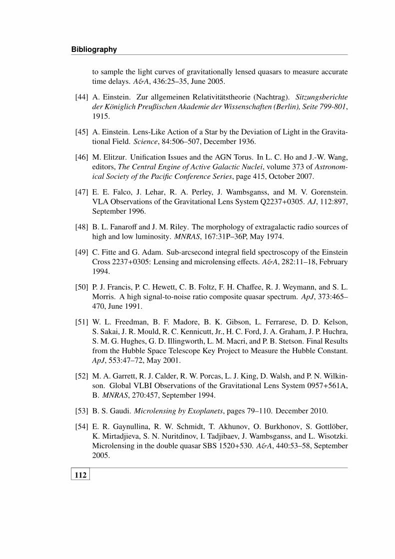
Bibliography
to sample the light curves of gravitationally lensed quasars to measure accuratetime delays. A&A, 436:25–35, June 2005.
[44] A. Einstein. Zur allgemeinen Relativitatstheorie (Nachtrag). Sitzungsberichteder Koniglich Preußischen Akademie der Wissenschaften (Berlin), Seite 799-801,1915.
[45] A. Einstein. Lens-Like Action of a Star by the Deviation of Light in the Gravita-tional Field. Science, 84:506–507, December 1936.
[46] M. Elitzur. Unification Issues and the AGN Torus. In L. C. Ho and J.-W. Wang,editors, The Central Engine of Active Galactic Nuclei, volume 373 of Astronom-ical Society of the Pacific Conference Series, page 415, October 2007.
[47] E. E. Falco, J. Lehar, R. A. Perley, J. Wambsganss, and M. V. Gorenstein.VLA Observations of the Gravitational Lens System Q2237+0305. AJ, 112:897,September 1996.
[48] B. L. Fanaroff and J. M. Riley. The morphology of extragalactic radio sources ofhigh and low luminosity. MNRAS, 167:31P–36P, May 1974.
[49] C. Fitte and G. Adam. Sub-arcsecond integral field spectroscopy of the EinsteinCross 2237+0305: Lensing and microlensing effects. A&A, 282:11–18, February1994.
[50] P. J. Francis, P. C. Hewett, C. B. Foltz, F. H. Chaffee, R. J. Weymann, and S. L.Morris. A high signal-to-noise ratio composite quasar spectrum. ApJ, 373:465–470, June 1991.
[51] W. L. Freedman, B. F. Madore, B. K. Gibson, L. Ferrarese, D. D. Kelson,S. Sakai, J. R. Mould, R. C. Kennicutt, Jr., H. C. Ford, J. A. Graham, J. P. Huchra,S. M. G. Hughes, G. D. Illingworth, L. M. Macri, and P. B. Stetson. Final Resultsfrom the Hubble Space Telescope Key Project to Measure the Hubble Constant.ApJ, 553:47–72, May 2001.
[52] M. A. Garrett, R. J. Calder, R. W. Porcas, L. J. King, D. Walsh, and P. N. Wilkin-son. Global VLBI Observations of the Gravitational Lens System 0957+561A,B. MNRAS, 270:457, September 1994.
[53] B. S. Gaudi. Microlensing by Exoplanets, pages 79–110. December 2010.
[54] E. R. Gaynullina, R. W. Schmidt, T. Akhunov, O. Burkhonov, S. Gottlober,K. Mirtadjieva, S. N. Nuritdinov, I. Tadjibaev, J. Wambsganss, and L. Wisotzki.Microlensing in the double quasar SBS 1520+530. A&A, 440:53–58, September2005.
112
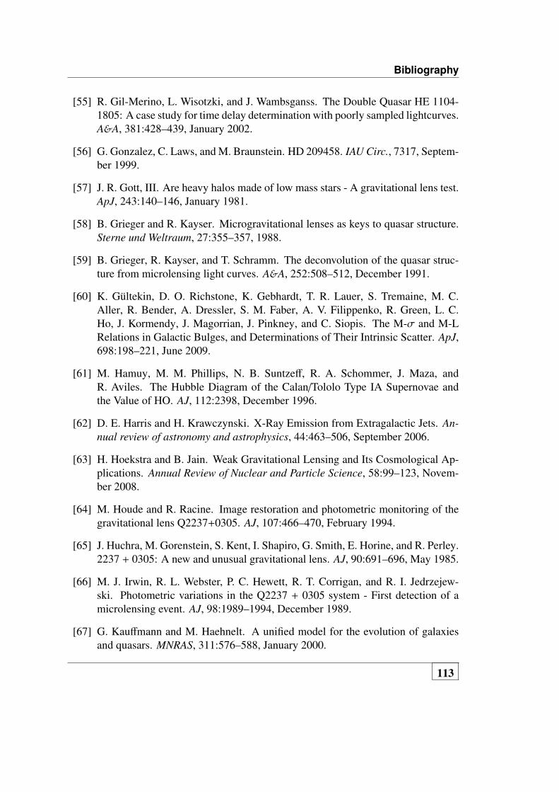
Bibliography
[55] R. Gil-Merino, L. Wisotzki, and J. Wambsganss. The Double Quasar HE 1104-1805: A case study for time delay determination with poorly sampled lightcurves.A&A, 381:428–439, January 2002.
[56] G. Gonzalez, C. Laws, and M. Braunstein. HD 209458. IAU Circ., 7317, Septem-ber 1999.
[57] J. R. Gott, III. Are heavy halos made of low mass stars - A gravitational lens test.ApJ, 243:140–146, January 1981.
[58] B. Grieger and R. Kayser. Microgravitational lenses as keys to quasar structure.Sterne und Weltraum, 27:355–357, 1988.
[59] B. Grieger, R. Kayser, and T. Schramm. The deconvolution of the quasar struc-ture from microlensing light curves. A&A, 252:508–512, December 1991.
[60] K. Gultekin, D. O. Richstone, K. Gebhardt, T. R. Lauer, S. Tremaine, M. C.Aller, R. Bender, A. Dressler, S. M. Faber, A. V. Filippenko, R. Green, L. C.Ho, J. Kormendy, J. Magorrian, J. Pinkney, and C. Siopis. The M-σ and M-LRelations in Galactic Bulges, and Determinations of Their Intrinsic Scatter. ApJ,698:198–221, June 2009.
[61] M. Hamuy, M. M. Phillips, N. B. Suntzeff, R. A. Schommer, J. Maza, andR. Aviles. The Hubble Diagram of the Calan/Tololo Type IA Supernovae andthe Value of HO. AJ, 112:2398, December 1996.
[62] D. E. Harris and H. Krawczynski. X-Ray Emission from Extragalactic Jets. An-nual review of astronomy and astrophysics, 44:463–506, September 2006.
[63] H. Hoekstra and B. Jain. Weak Gravitational Lensing and Its Cosmological Ap-plications. Annual Review of Nuclear and Particle Science, 58:99–123, Novem-ber 2008.
[64] M. Houde and R. Racine. Image restoration and photometric monitoring of thegravitational lens Q2237+0305. AJ, 107:466–470, February 1994.
[65] J. Huchra, M. Gorenstein, S. Kent, I. Shapiro, G. Smith, E. Horine, and R. Perley.2237 + 0305: A new and unusual gravitational lens. AJ, 90:691–696, May 1985.
[66] M. J. Irwin, R. L. Webster, P. C. Hewett, R. T. Corrigan, and R. I. Jedrzejew-ski. Photometric variations in the Q2237 + 0305 system - First detection of amicrolensing event. AJ, 98:1989–1994, December 1989.
[67] G. Kauffmann and M. Haehnelt. A unified model for the evolution of galaxiesand quasars. MNRAS, 311:576–588, January 2000.
113

Bibliography
[68] R. Kayser. Micro gravitation lenses and their significance for astrophysics. Sterneund Weltraum, 25:252–254, May 1986.
[69] R. Kayser and S. Refsdal. Detectability of gravitational microlensing in thequasar QSO2237 + 0305. Nature, 338:745, April 1989.
[70] A. G. Kim, S. Gabi, G. Goldhaber, D. E. Groom, I. M. Hook, M. Y. Kim, J. C.Lee, C. R. Pennypacker, S. Perlmutter, I. A. Small, A. Goobar, R. Pain, R. S. Ellis,R. G. McMahon, B. J. Boyle, P. S. Bunclark, D. Carter, M. J. Irwin, K. Glaze-brook, H. J. M. Newberg, A. V. Filippenko, T. Matheson, M. Dopita, W. J. Couch,and (. S. C. Project). Implications for the Hubble Constant from the First SevenSupernovae at z >= 0.35. ApJL, 476:L63–L66, February 1997.
[71] C. S. Kochanek. What Do Gravitational Lens Time Delays Measure? ApJ,578:25–32, October 2002.
[72] C. S. Kochanek. Quantitative Interpretation of Quasar Microlensing LightCurves. ApJ, 605:58–77, April 2004.
[73] C. S. Kochanek, N. D. Morgan, E. E. Falco, B. A. McLeod, J. N. Winn, J. Dem-bicky, and B. Ketzeback. The Time Delays of Gravitational Lens HE 0435-1223:An Early-Type Galaxy with a Rising Rotation Curve. ApJ, 640:47–61, March2006.
[74] L. V. E. Koopmans and CLASS Collaboration. The Hubble Constant from(CLASS) Gravitational Lenses. Publications of the Astronomical Society of Aus-tralia, 18:179–181, 2001.
[75] E. Koptelova, W. P. Chen, T. Chiueh, B. P. Artamonov, V. L. Oknyanskij, S. N.Nuritdinov, O. Burkhonov, T. Akhunov, V. V. Bruevich, O. V. Ezhkova, A. S.Gusev, A. V. Sergeyev, S. A. Ehgamberdiev, and M. A. Ibragimov. Time delaybetween images of the lensed quasar UM673. A&A, 544:A51, August 2012.
[76] E. Koptelova, V. Oknyanskij, B. Artamonov, and W.-P. Chen. Multiwavelengthsobservations of lensed quasars: interband time delays. Memorie della SocietaAstronomica Italiana, 81:138, 2010.
[77] E. A. Koptelova, V. L. Oknyanskij, and E. V. Shimanovskaya. Determining timedelay in the gravitationally lensed system QSO2237+0305. A&A, 452:37–46,June 2006.
[78] A. Koratkar and O. Blaes. The Ultraviolet and Optical Continuum Emission inActive Galactic Nuclei: The Status of Accretion Disks. PASP, 111:1–30, January1999.
114

Bibliography
[79] J. Kormendy and R. C. Kennicutt, Jr. Secular Evolution and the Formation ofPseudobulges in Disk Galaxies. Annual review of astronomy and astrophysics,42:603–683, September 2004.
[80] H. Krawczynski and E. Treister. Active galactic nuclei the physics of individualsources and the cosmic history of formation and evolution. Frontiers of Physics,8:609–629, December 2013.
[81] T. Kundic, E. L. Turner, W. N. Colley, J. R. Gott, III, J. E. Rhoads, Y. Wang,L. E. Bergeron, K. A. Gloria, D. C. Long, S. Malhotra, and J. Wambsganss. ARobust Determination of the Time Delay in 0957+561A, B and a Measurementof the Global Value of Hubble’s Constant. ApJ, 482:75–82, June 1997.
[82] D. W. Latham, R. P. Stefanik, T. Mazeh, M. Mayor, and G. Burki. The unseencompanion of HD114762 - A probable brown dwarf. Nature, 339:38–40, May1989.
[83] A. Lawrence. The relative frequency of broad-lined and narrow-lined activegalactic nuclei - Implications for unified schemes. MNRAS, 252:586–592, Oc-tober 1991.
[84] G. F. Lewis and K. E. Belle. Microlensing of broad absorption line quasars.MNRAS, 297:69–76, June 1998.
[85] G. F. Lewis and R. A. Ibata. Quasar Image Shifts Resulting from GravitationalMicrolensing. ApJ, 501:478–485, July 1998.
[86] G. F. Lewis and R. A. Ibata. Gravitational microlensing of quasar broad-lineregions at large optical depths. MNRAS, 348:24–33, February 2004.
[87] G. F. Lewis, M. J. Irwin, P. C. Hewett, and C. B. Foltz. Microlensing-inducedspectral variability in Q 2237+0305. MNRAS, 295:573, April 1998.
[88] M. S. Longair, M. Ryle, and P. A. G. Scheuer. Models of extended radiosources.MNRAS, 164:243, 1973.
[89] D. Lynden-Bell. Galactic Nuclei as Collapsed Old Quasars. Nature, 223:690–694, August 1969.
[90] G. M. MacAlpine and F. R. Feldman. Discovery and spectrophotometry of high-redshift quasars. ApJ, 261:412–421, October 1982.
[91] J. Machalski, D. Kozieł-Wierzbowska, M. Jamrozy, and D. J. Saikia. J1420-0545: The Radio Galaxy Larger than 3C 236. ApJ, 679:149–155, May 2008.
115

Bibliography
[92] J. Magorrian, S. Tremaine, D. Richstone, R. Bender, G. Bower, A. Dressler,S. M. Faber, K. Gebhardt, R. Green, C. Grillmair, J. Kormendy, and T. Lauer.The Demography of Massive Dark Objects in Galaxy Centers. AJ, 115:2285–2305, June 1998.
[93] A. Marconi, G. Risaliti, R. Gilli, L. K. Hunt, R. Maiolino, and M. Salvati. Localsupermassive black holes, relics of active galactic nuclei and the X-ray back-ground. MNRAS, 351:169–185, June 2004.
[94] R. Massey, T. Kitching, and J. Richard. The dark matter of gravitational lensing.Reports on Progress in Physics, 73(8):086901, August 2010.
[95] T. A. Matthews and A. R. Sandage. Optical Identification of 3c 48, 3c 196, and3c 286 with Stellar Objects. ApJ, 138:30, July 1963.
[96] B. A. McLeod, E. E. Falco, J. Lehar, C. D. Impey, C. S. Kochanek, C. Y. Peng,and H.-W. Rix. Lens galaxies revealed: highlights of the CASTLES lens survey.In American Astronomical Society Meeting Abstracts, volume 29 of Bulletin ofthe American Astronomical Society, page 1307, December 1997.
[97] B. R. McNamara and P. E. J. Nulsen. Mechanical feedback from active galacticnuclei in galaxies, groups and clusters. New Journal of Physics, 14(5):055023,May 2012.
[98] E. Mediavilla, J. Jimenez-Vicente, J. A. Munoz, and T. Mediavilla. Resolvingthe Innermost Region of the Accretion Disk of the Lensed Quasar Q2237+0305through Gravitational Microlensing. ApJL, 814:L26, December 2015.
[99] R. B. Metcalf and H. Zhao. Flux Ratios as a Probe of Dark Substructures inQuadruple-Image Gravitational Lenses. ApJL, 567:L5–L8, March 2002.
[100] B. Moore, N. Katz, G. Lake, A. Dressler, and A. Oemler. Galaxy harassment andthe evolution of clusters of galaxies. Nature, 379:613–616, February 1996.
[101] O. Moreau, C. Libbrecht, D.-W. Lee, and J. Surdej. Accurate photometric lightcurves of the lensed components of Q2237+0305 derived with an optimal imagesubtraction technique: Evidence for microlensing in image A. A&A, 436:479–492, June 2005.
[102] N. D. Morgan, J. A. R. Caldwell, P. L. Schechter, A. Dressler, E. Egami, andH.-W. Rix. WFI J2026-4536 and WFI J2033-4723: Two New Quadruple Gravi-tational Lenses. AJ, 127:2617–2630, May 2004.
116

Bibliography
[103] D. J. Mortlock, S. J. Warren, B. P. Venemans, M. Patel, P. C. Hewett, R. G.McMahon, C. Simpson, T. Theuns, E. A. Gonzales-Solares, A. Adamson, S. Dye,N. C. Hambly, P. Hirst, M. J. Irwin, E. Kuiper, A. Lawrence, and H. J. A. Rottger-ing. A luminous quasar at a redshift of z = 7.085. Nature, 474:616–619, June2011.
[104] M. J. Mortonson, P. L. Schechter, and J. Wambsganss. Size Is Everything: Uni-versal Features of Quasar Microlensing with Extended Sources. ApJ, 628:594–603, August 2005.
[105] D. Nadeau, H. K. C. Yee, W. J. Forrest, J. D. Garnett, Z. Ninkov, and J. L. Pipher.Infrared and visible photometry of the gravitational lens systems 2237 + 030.ApJ, 376:430–438, August 1991.
[106] M. Nenkova, M. M. Sirocky, Z. Ivezic, and M. Elitzur. AGN Dusty Tori. I.Handling of Clumpy Media. ApJ, 685:147–159, September 2008.
[107] E. O. Ofek, D. Maoz, H.-W. Rix, C. S. Kochanek, and E. E. Falco. SpectroscopicRedshifts for Seven Lens Galaxies. ApJ, 641:70–77, April 2006.
[108] R. Ostensen, S. Refsdal, R. Stabell, J. Teuber, P. I. Emanuelsen, L. Festin,R. Florentin-Nielsen, G. Gahm, E. Gullbring, F. Grundahl, J. Hjorth, M. Jablon-ski, A. O. Jaunsen, A. A. Kaas, H. Karttunen, J. Kotilainen, E. Laurikainen,H. Lindgren, P. Maehoenen, K. Nilsson, G. Olofsson, O. Olsen, B. R. Pettersen,V. Piirola, A. N. Sorensen, L. Takalo, B. Thomsen, E. Valtaoja, M. Vestergaard,and T. Av Vianborg. Monitoring of the Einstein Cross with the Nordic OpticalTelescope. A&A, 309:59–64, May 1996.
[109] B. Paczynski. Gravitational microlensing at large optical depth. ApJ, 301:503–516, February 1986.
[110] B. Paczynski. Gravitational microlensing by the galactic halo. ApJ, 304:1–5,May 1986.
[111] B. Paczynski and A. Udalski. Optical Gravtational Lensing Experiment (OGLE).IAU Circ., 5997, May 1994.
[112] R. Pello, B. Sanahuja, J.-F. Le Borgne, G. Soucail, and Y. Mellier. A straightgravitational image in Abell 2390 - A striking case of lensing by a cluster ofgalaxies. ApJ, 366:405–411, January 1991.
[113] J. Pelt, R. Kayser, S. Refsdal, and T. Schramm. The light curve and the timedelay of QSO 0957+561. A&A, 305:97, January 1996.
117
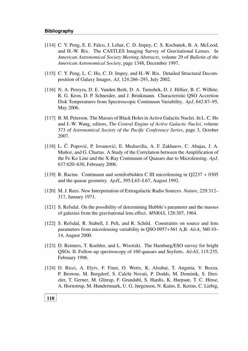
Bibliography
[114] C. Y. Peng, E. E. Falco, J. Lehar, C. D. Impey, C. S. Kochanek, B. A. McLeod,and H.-W. Rix. The CASTLES Imaging Survey of Gravitational Lenses. InAmerican Astronomical Society Meeting Abstracts, volume 29 of Bulletin of theAmerican Astronomical Society, page 1348, December 1997.
[115] C. Y. Peng, L. C. Ho, C. D. Impey, and H.-W. Rix. Detailed Structural Decom-position of Galaxy Images. AJ, 124:266–293, July 2002.
[116] N. A. Pereyra, D. E. Vanden Berk, D. A. Turnshek, D. J. Hillier, B. C. Wilhite,R. G. Kron, D. P. Schneider, and J. Brinkmann. Characteristic QSO AccretionDisk Temperatures from Spectroscopic Continuum Variability. ApJ, 642:87–95,May 2006.
[117] B. M. Peterson. The Masses of Black Holes in Active Galactic Nuclei. In L. C. Hoand J.-W. Wang, editors, The Central Engine of Active Galactic Nuclei, volume373 of Astronomical Society of the Pacific Conference Series, page 3, October2007.
[118] L. C. Popovic, P. Jovanovic, E. Mediavilla, A. F. Zakharov, C. Abajas, J. A.Munoz, and G. Chartas. A Study of the Correlation between the Amplification ofthe Fe Kα Line and the X-Ray Continuum of Quasars due to Microlensing. ApJ,637:620–630, February 2006.
[119] R. Racine. Continuum and semiforbidden C III microlensing in Q2237 + 0305and the quasar geometry. ApJL, 395:L65–L67, August 1992.
[120] M. J. Rees. New Interpretation of Extragalactic Radio Sources. Nature, 229:312–317, January 1971.
[121] S. Refsdal. On the possibility of determining Hubble’s parameter and the massesof galaxies from the gravitational lens effect. MNRAS, 128:307, 1964.
[122] S. Refsdal, R. Stabell, J. Pelt, and R. Schild. Constraints on source and lensparameters from microlensing variability in QSO 0957+561 A,B. A&A, 360:10–14, August 2000.
[123] D. Reimers, T. Koehler, and L. Wisotzki. The Hamburg/ESO survey for brightQSOs. II. Follow-up spectroscopy of 160 quasars and Seyferts. A&AS, 115:235,February 1996.
[124] D. Ricci, A. Elyiv, F. Finet, O. Wertz, K. Alsubai, T. Anguita, V. Bozza,P. Browne, M. Burgdorf, S. Calchi Novati, P. Dodds, M. Dominik, S. Drei-zler, T. Gerner, M. Glitrup, F. Grundahl, S. Hardis, K. Harpsøe, T. C. Hinse,A. Hornstrup, M. Hundertmark, U. G. Jørgensen, N. Kains, E. Kerins, C. Liebig,
118
Bibliography
G. Maier, L. Mancini, G. Masi, M. Mathiasen, M. Penny, S. Proft, S. Rah-var, G. Scarpetta, K. Sahu, S. Schafer, F. Schonebeck, R. Schmidt, J. Skottfelt,C. Snodgrass, J. Southworth, C. C. Thone, J. Wambsganss, F. Zimmer, M. Zub,and J. Surdej. Flux and color variations of the doubly imaged quasar UM673.A&A, 551:A104, March 2013.
[125] D. Ricci, J. Poels, A. Elyiv, F. Finet, P. G. Sprimont, T. Anguita, V. Bozza,P. Browne, M. Burgdorf, S. Calchi Novati, M. Dominik, S. Dreizler, M. Glitrup,F. Grundahl, K. Harpsøe, F. Hessman, T. C. Hinse, A. Hornstrup, M. Hundert-mark, U. G. Jørgensen, C. Liebig, G. Maier, L. Mancini, G. Masi, M. Mathiasen,S. Rahvar, G. Scarpetta, J. Skottfelt, C. Snodgrass, J. Southworth, J. Teuber, C. C.Thone, J. Wambsganß, F. Zimmer, M. Zub, and J. Surdej. Flux and color vari-ations of the quadruply imaged quasar HE 0435-1223. A&A, 528:A42, April2011.
[126] G. T. Richards, C. R. Keeton, B. Pindor, J. F. Hennawi, P. B. Hall, E. L. Turner,N. Inada, M. Oguri, S.-I. Ichikawa, R. H. Becker, M. D. Gregg, R. L. White,J. S. B. Wyithe, D. P. Schneider, D. E. Johnston, J. A. Frieman, and J. Brinkmann.Microlensing of the Broad Emission Line Region in the Quadruple Lens SDSSJ1004+4112. ApJ, 610:679–685, August 2004.
[127] H.-W. Rix, D. P. Schneider, and J. N. Bahcall. Hubble Space Telescope WideField Camera imaging of the gravitational lens 2237 + 0305. AJ, 104:959–967,September 1992.
[128] D. B. Sanders, B. T. Soifer, J. H. Elias, B. F. Madore, K. Matthews, G. Neuge-bauer, and N. Z. Scoville. Ultraluminous infrared galaxies and the origin ofquasars. ApJ, 325:74–91, February 1988.
[129] A. B. Saust. Determining the size of the emission line region in Q2237+031 frommicrolensing. A&AS, 103, January 1994.
[130] P. L. Schechter and J. Wambsganss. Quasar Microlensing at High Magnifica-tion and the Role of Dark Matter: Enhanced Fluctuations and Suppressed SaddlePoints. ApJ, 580:685–695, December 2002.
[131] P. A. G. Scheuer. Models of extragalactic radio sources with a continuous energysupply from a central object. MNRAS, 166:513–528, March 1974.
[132] M. Schmidt. 3C 273 : A Star-Like Object with Large Red-Shift. Nature,197:1040, March 1963.
[133] R. Schmidt, R. L. Webster, and G. F. Lewis. Weighing a galaxy bar in the lensQ2237 + 0305. MNRAS, 295:488, April 1998.
119

Bibliography
[134] R. W. Schmidt and J. Wambsganss. Quasar microlensing. General Relativity andGravitation, 42:2127–2150, September 2010.
[135] D. P. Schneider, E. L. Turner, J. E. Gunn, J. N. Hewitt, M. Schmidt, and C. R.Lawrence. Erratum: High-Resolution CCD Imaging and Derived GravitationalLens Models of 2237+0305 (A.J. 95, 1619 (1988). AJ, 96:1755, November 1988.
[136] P. Schneider. A new formulation of gravitational lens theory, time-delay, andFermat’s principle. A&A, 143:413–420, February 1985.
[137] P. Schneider and J. Wambsganss. Are the broad emission lines of quasars affectedby gravitational microlensing? A&A, 237:42–53, October 1990.
[138] N. I. Shakura and R. A. Sunyaev. Black holes in binary systems. Observationalappearance. A&A, 24:337–355, 1973.
[139] F. Shankar, P. Salucci, G. L. Granato, G. De Zotti, and L. Danese. Supermassiveblack hole demography: the match between the local and accreted mass func-tions. MNRAS, 354:1020–1030, November 2004.
[140] G. A. Shields. Thermal continuum from acretion disks in quasars. Nature,272:706–708, April 1978.
[141] D. Sluse, M. Kishimoto, T. Anguita, O. Wucknitz, and J. Wambsganss. Mid-infrared microlensing of accretion disc and dusty torus in quasars: effects on fluxratio anomalies. A&A, 553:A53, May 2013.
[142] A. Smette, J. Surdej, P. A. Shaver, C. B. Foltz, F. H. Chaffee, R. J. Weymann,R. E. Williams, and P. Magain. A spectroscopic study of UM 673 A and B - Onthe size of Lyman-alpha clouds. ApJ, 389:39–62, April 1992.
[143] A. Soltan. Masses of quasars. MNRAS, 200:115–122, July 1982.
[144] L. S. Sparke and J. S. Gallagher, III. Galaxies in the Universe. February 2007.
[145] J. Surdej, P. Magain, J.-P. Swings, U. Borgeest, T. J.-L. Courvoisier, R. Kayer,K. I. Kellermann, H. Kuhr, and S. Refsdal. Observations of the new gravitationallens system UM 673 = Q 0142-100. A&A, 198:49–60, June 1988.
[146] J. Surdej, P. Magain, J.-P. Swings, U. Borgeest, T. J.-L. Courvoisier, R. Kayser,K. I. Kellermann, H. Kuhr, and S. Refsdal. A new case of gravitational lensing.Nature, 329:695, October 1987.
[147] M. Tewes, F. Courbin, and G. Meylan. COSMOGRAIL: the COSmologicalMOnitoring of GRAvItational Lenses. XI. Techniques for time delay measure-ment in presence of microlensing. A&A, 553:A120, May 2013.
120

Bibliography
[148] E. Treister, P. Natarajan, D. B. Sanders, C. M. Urry, K. Schawinski, and J. Kar-taltepe. Major Galaxy Mergers and the Growth of Supermassive Black Holes inQuasars. Science, 328:600, April 2010.
[149] E. Treister, K. Schawinski, C. M. Urry, and B. D. Simmons. Major Galaxy Merg-ers Only Trigger the Most Luminous Active Galactic Nuclei. ApJL, 758:L39,October 2012.
[150] E. Treister and C. M. Urry. The Evolution of Obscuration in Active GalacticNuclei. ApJL, 652:L79–L82, December 2006.
[151] E. Treister, C. M. Urry, and S. Virani. The Space Density of Compton-ThickActive Galactic Nucleus and the X-Ray Background. ApJ, 696:110–120, May2009.
[152] M. Treyer and J. Wambsganss. Astrometric microlensing of quasars. Dependenceon surface mass density and external shear. A&A, 416:19–34, March 2004.
[153] A. Udalski, M. K. Szymanski, M. Kubiak, G. Pietrzynski, I. Soszynski, K. Ze-brun, O. Szewczyk, L. Wyrzykowski, K. Ulaczyk, and T. Wieckowski. The Op-tical Gravitational Lensing Experiment. OGLE-III Long Term Monitoring of theGravitational Lens QSO 2237+0305. Acta Astronomica, 56:293–305, December2006.
[154] V. Vakulik, R. Schild, V. Dudinov, S. Nuritdinov, V. Tsvetkova, O. Burkhonov,and T. Akhunov. Observational determination of the time delays in gravitationallens system Q2237+0305. A&A, 447:905–913, March 2006.
[155] V. G. Vakulik, V. N. Dudinov, A. P. Zheleznyak, V. S. Tsvetkova, P. Notni,V. N. Shalyapin, and B. P. Artamonov. VRI photometry of the Einstein CrossQ2237+0305 at Maidanak observatory. Astronomische Nachrichten, 318:73,February 1997.
[156] V. G. Vakulik, R. E. Schild, V. N. Dudinov, A. A. Minakov, S. N. Nuritdinov, V. S.Tsvetkova, A. P. Zheleznyak, V. V. Konichek, I. Y. Sinelnikov, O. A. Burkhonov,B. P. Artamonov, and V. V. Bruevich. Color effects associated with the 1999 mi-crolensing brightness peaks in gravitationally lensed quasar Q2237+0305. A&A,420:447–457, June 2004.
[157] D. E. Vanden Berk, B. C. Wilhite, R. G. Kron, S. F. Anderson, R. J. Brunner, P. B.Hall, Z. Ivezic, G. T. Richards, D. P. Schneider, D. G. York, J. V. Brinkmann,D. Q. Lamb, R. C. Nichol, and D. J. Schlegel. The Ensemble Photometric Vari-ability of ˜25,000 Quasars in the Sloan Digital Sky Survey. ApJ, 601:692–714,February 2004.
121

Bibliography
[158] C. Vuissoz, F. Courbin, D. Sluse, G. Meylan, V. Chantry, E. Eulaers, C. Morgan,M. E. Eyler, C. S. Kochanek, J. Coles, P. Saha, P. Magain, and E. E. Falco.COSMOGRAIL: the COSmological MOnitoring of GRAvItational Lenses. VII.Time delays and the Hubble constant from WFI J2033-4723. A&A, 488:481–490,September 2008.
[159] D. Walsh, R. F. Carswell, and R. J. Weymann. 0957 + 561 A, B - Twin quasistel-lar objects or gravitational lens. Nature, 279:381–384, May 1979.
[160] J. Wambsganss. Gravitational Microlensing. ArXiv Astrophysics e-prints, April2006.
[161] J. Wambsganss and B. Paczynski. Expected color variations of the gravitationallymicrolensed QSO 2237 + 0305. AJ, 102:864–868, September 1991.
[162] J. Wambsganss and B. Paczynski. A direct gravitational lensing test for 10 exp6 solar masses black holes in halos of galaxies. ApJL, 397:L1–L4, September1992.
[163] J. Wambsganss and B. Paczynski. Parameter degeneracy in models of the quadru-ple lens system Q2237+0305. AJ, 108:1156–1162, October 1994.
[164] J. Wambsganss, B. Paczynski, and P. Schneider. Interpretation of the microlens-ing event in QSO 2237 + 0305. ApJL, 358:L33–L36, August 1990.
[165] J. Wambsganss, R. W. Schmidt, W. Colley, T. Kundic, and E. L. Turner. Mi-crolensing results from APO monitoring of the double quasar Q0957+561A,Bbetween 1995 and 1998. A&A, 362:L37–L40, October 2000.
[166] L. L. R. Williams and P. Saha. Improper Motions in Lensed QSOs. AJ, 110:1471,October 1995.
[167] C. J. Willott, L. Albert, D. Arzoumanian, J. Bergeron, D. Crampton, P. Delorme,J. B. Hutchings, A. Omont, C. Reyle, and D. Schade. Eddington-limited Accre-tion and the Black Hole Mass Function at Redshift 6. AJ, 140:546–560, August2010.
[168] L. Wisotzki, T. Becker, L. Christensen, A. Helms, K. Jahnke, A. Kelz, M. M.Roth, and S. F. Sanchez. Integral-field spectrophotometry of the quadruple QSOHE 0435-1223: Evidence for microlensing. A&A, 408:455–463, September2003.
[169] L. Wisotzki, N. Christlieb, N. Bade, V. Beckmann, T. Kohler, C. Vanelle, andD. Reimers. The Hamburg/ESO survey for bright QSOs. III. A large flux-limitedsample of QSOs. A&A, 358:77–87, June 2000.
122

Bibliography
[170] L. Wisotzki, T. Koehler, D. Groote, and D. Reimers. The Hamburg/ESO surveyfor bright QSOs. I. Survey design and candidate selection procedure. A&AS,115:227, February 1996.
[171] L. Wisotzki, P. L. Schechter, H. V. Bradt, J. Heinmuller, and D. Reimers. HE0435-1223: A wide separation quadruple QSO and gravitational lens. A&A,395:17–23, November 2002.
[172] L. Wisotzki, P. L. Schechter, H.-W. Chen, D. Richstone, K. Jahnke, S. F. Sanchez,and D. Reimers. HE 0047-1756: A new gravitationally lensed double QSO. A&A,419:L31–L34, May 2004.
[173] P. R. Wozniak, C. Alard, A. Udalski, M. Szymanski, M. Kubiak, G. Pietrzynski,and K. Zebrun. The Optical Gravitational Lensing Experiment Monitoring ofQSO 2237+0305. ApJ, 529:88–92, January 2000.
[174] P. R. Wozniak, A. Udalski, M. Szymanski, M. Kubiak, G. Pietrzynski,I. Soszynski, and K. Zebrun. The Optical Gravitational Lensing Experiment: AHunt for Caustic Crossings in QSO 2237+0305. ApJL, 540:L65–L67, September2000.
[175] J. S. B. Wyithe, R. L. Webster, and E. L. Turner. A small source in Q2237+0305?MNRAS, 318:762–768, November 2000.
[176] R.-z. Yang, N. Sahakyan, E. D. O. Wilhelmi, F. Aharonian, and F. Rieger. Deepobservation of the giant radio lobes of Centaurus A with the Fermi large areatelescope. In F. A. Aharonian, W. Hofmann, and F. M. Rieger, editors, Ameri-can Institute of Physics Conference Series, volume 1505 of American Institute ofPhysics Conference Series, pages 590–593, December 2012.
[177] H. K. C. Yee. High-resolution imaging of the gravitational lens system candidate2237+030. AJ, 95:1331–1339, May 1988.
[178] A. Yonehara. Evidence for a Source Size of Less than 2000 AU in Quasar2237+0305. ApJL, 548:L127–L130, February 2001.
[179] A. Yonehara, S. Mineshige, T. Manmoto, J. Fukue, M. Umemura, and E. L.Turner. An X-Ray Microlensing Test of AU-Scale Accretion Disk Structure inQ2237+0305. ApJL, 501:L41–L44, July 1998.
[180] P. Young, J. E. Gunn, J. B. Oke, J. A. Westphal, and J. Kristian. Q0957+561 -Detailed models of the gravitational lens effect. ApJ, 244:736–755, March 1981.
[181] F. Zwicky. Nebulae as Gravitational Lenses. Physical Review, 51:290–290,February 1937.
123

Bibliography
[182] F. Zwicky. On the Probability of Detecting Nebulae Which Act as GravitationalLenses. Physical Review, 51:679–679, April 1937.
124

Acknowledgements
Apparently I made it to the end against the odds.And if this happened it is just because of a few very special people I met on my way.It’s the time to say thank you to everyone has accompanied and sometimes, I’d dare say,pushed me through this long journey.I would like to thank my supervisor Professor Joachim Wambsganß for advice, supportduring all the stages of this work, and for the infinite and unique understanding regard-ing my private life events.I owe my deepest gratitude to Dr. Robert W. Schmidt for help, suggestions, support,computational advice, especially when it seemed that our project had led us to what weused to define a “Cul-de-sac”. Thank you for always being so enthusiastic about the“Quasar microlensing business” and having helped me digging into dirt!A special thank you goes to Dr. Anna Pasquali, the backbone of the second floor at theARI Neubau. My time at ARI would have been much sadder without having such acheerful person next door. Thanks for the scientifical support and the funny chats, theshortest lunches of our lives and the shopaholic Saturdays.Thanks to Christiane, Frederik, Clio and Giulio for having shared their time and thoughtswith me at the ARI coffee breaks.A special thanks goes to Federica e Alessandra. Due forze della natura. You made melaugh so much.Thanks to all the fellows of this adventure, the 7th IMPRS generation, for sharing withme their triumphs and despair.Anahı and Jan, you made my life easier and nicer more than once.A special thank you goes to my officemate, Svea, for useful discussions, for helping mefilling up otherwise unbearable german forms, and for keeping each other very goodcompany.Eleonora, grazie della tua presenza confortante e della tua ironia.Camilla, la mia vicina di casa. Mi hai aiutato tanto nel momento del bisogno e offertoun’altra finestra sul mondo.Agnese I am grateful for having met you on that airplane. We went through a longjourney together and I am not going to forget all the things we shared, la disperazione,l’aridita e la passione per i dolci. Grazie della tua dolcezza e mitezza.Many many special thanks to my flatmates: Anja, Jassi, Isa. I very much enjoyed ourWG trips and reunions through Germany after we had to split up.Grazie a Martina, tra le poche certezze di questa vita.Un ringraziamento speciale va alla mia famiglia, Ennio, Marina e Clarissa, il cui sup-porto mi ha aiutato a varcare il traguardo. Grazie per l’incalcolabile aiuto che mi offritementre attraverso un momento difficile.Un grazie speciale va infine al mio caro Luca, per essere sempre e comunque al miofianco, e spronarmi a vedere quella lucina giu in fondo.
125


List of Publications
[1] Giannini E. and Lunine J.I. Microlensing detection of extrasolar planets. Reports onProgress in Physics, 76, May 2013.
[2] Giannini E. et al. MiNDSTEp differential photometry of the gravitationally lensedquasars WFI2033-4723 and HE0047-1756: Microlensing and a new time delay. Ac-cepted for publication in A&A.
[3-9] MiNDSTEp member in 2012 and coauthor of a series of papers published by theMiNDSTEp collaboration since 2013.
127


Statement of Authorship -Selbstandigkeitserklarung
Ich, Emanuela Giannini, versichere, dass ich die vorgelegte Dissertation selbststandigverfasst habe und keine anderen als die angegebenen Quellen und Hilfsmittel benutzthabe.
129