electron transport in nano devices mathematical introduction and...
TRANSCRIPT

ELECTRON TRANSPORT IN NANO DEVICESMATHEMATICAL INTRODUCTION AND
PRECONDITIONING
Olga Trichtchenko
Master of Science
Department of Mathematics and Statistics
McGill University
Montreal, Quebec
June 15, 2009
A thesis submitted to McGill University in partial fulfilment of therequirements of the degree of Master of Science
c© Olga Trichtchenko, 2009

ACKNOWLEDGEMENTS
I thank my supervisor and the students at both McGill and my temporary
home, SFU. I also thank my family and my friends for their support.
ii

ABSTRACT
In this thesis we outline the mathematical principles behind density func-
tional theory, and describe the iterative Kohn-Sham formulation for compu-
tation of electronic density calculations in nano devices. The model for com-
putation of the density of electrons in such device is a non-linear eigenvalue
problem that is solved iteratively using the resolvent formalism. There are
several bottlenecks to this approach and we propose methods to resolve them.
This iterative method involves a matrix inversion. This matrix inversion is
called upon when calculating the Green’s function for a particular system, the
two-probe device. A method to speed up this calculation is to use a precondi-
tioning technique to accelerate the convergence of the iterative method. Tests
the existing algorithm for a one-dimensional system are presented. The results
indicate that these preconditioning methods reduce the condition number of
the matrices.
iii

RESUME
Dans cette these, nous presentons les principes mathematiques a la base de
la theorie de la fonctionnelle de la densite, et nous decrivons la formule Kohn-
Sham iterative pour le calcul des densites d’electron dans les composants nano-
electroniques. Le modele de densite electronique est un probleme de valeur-
propre non-lineaire que l’on resout de maniere iterative. Il y a plusieurs compli-
cations liees a cette technique et nous proposons des methodes pour y remedier.
On formule le systeme a l’aide du calcul de l’operateur hamiltonien dans une
base particuliere. Cette inversion de matrice est necessaire lors du calcul de
la fonction de Green pour le systeme en question: l’appareil a deux sondes.
Afin d’accelerer ce calcul, nous utilisons une technique de preconditionnement
basee sur la nature iterative du probleme. Nous presentons les resultats de nos
essais avec differents preconditionneurs. Ceux-ci indiquent que ces methodes
reduisent le nombre de conditionnement de notre matrice. Ce preconditionnement
est donc applique a des algorithmes d’inversion iteratives classiques tels que
la methode de Gauss-Seidel et la methode du residu minimal generalisee. En
effet, nous observons une reduction du nombre d’iterations necessaires pour le
calcul de la matrice inverse.
iv

TABLE OF CONTENTS
ACKNOWLEDGEMENTS . . . . . . . . . . . . . . . . . . . . . . . . ii
ABSTRACT . . . . . . . . . . . . . . . . . . . . . . . . . . . . . . . . iii
RESUME . . . . . . . . . . . . . . . . . . . . . . . . . . . . . . . . . . iv
LIST OF TABLES . . . . . . . . . . . . . . . . . . . . . . . . . . . . . vii
LIST OF FIGURES . . . . . . . . . . . . . . . . . . . . . . . . . . . . viii
1 Introduction . . . . . . . . . . . . . . . . . . . . . . . . . . . . . . 1
1.1 Overview . . . . . . . . . . . . . . . . . . . . . . . . . . . . 2
2 Density Functional Theory . . . . . . . . . . . . . . . . . . . . . . 5
2.1 Overview . . . . . . . . . . . . . . . . . . . . . . . . . . . . 52.2 The Hamiltonian . . . . . . . . . . . . . . . . . . . . . . . 52.3 Density Functional Theory . . . . . . . . . . . . . . . . . . 62.4 Variational Principle . . . . . . . . . . . . . . . . . . . . . 92.5 Full Energy Functional . . . . . . . . . . . . . . . . . . . . 10
2.5.1 Hartree Potential, UH . . . . . . . . . . . . . . . . . 112.5.2 Exchange-Correlation Potential, UXC . . . . . . . . 12
2.6 Summary . . . . . . . . . . . . . . . . . . . . . . . . . . . 13
3 Green’s Functions and Density . . . . . . . . . . . . . . . . . . . . 14
3.1 Overview . . . . . . . . . . . . . . . . . . . . . . . . . . . . 143.2 Green’s Functions . . . . . . . . . . . . . . . . . . . . . . . 143.3 Density . . . . . . . . . . . . . . . . . . . . . . . . . . . . . 17
3.3.1 Contour Integration . . . . . . . . . . . . . . . . . . 173.3.2 Integration Along Real Axis . . . . . . . . . . . . . 19
3.4 General Formalism . . . . . . . . . . . . . . . . . . . . . . 213.5 Approximations . . . . . . . . . . . . . . . . . . . . . . . . 243.6 Summary . . . . . . . . . . . . . . . . . . . . . . . . . . . 24
4 Two Probe Device . . . . . . . . . . . . . . . . . . . . . . . . . . 26
4.1 Overview . . . . . . . . . . . . . . . . . . . . . . . . . . . . 264.2 Infinite System . . . . . . . . . . . . . . . . . . . . . . . . 264.3 Non-Equilibrium Eigenvalues . . . . . . . . . . . . . . . . . 29
v

4.4 Total Density . . . . . . . . . . . . . . . . . . . . . . . . . 314.4.1 Fermi Distribution . . . . . . . . . . . . . . . . . . . 314.4.2 Fermi-Dirac Statistics . . . . . . . . . . . . . . . . . 32
4.5 Self-Energies . . . . . . . . . . . . . . . . . . . . . . . . . . 344.5.1 Inverse of Block Tridiagonal Matrix . . . . . . . . . 344.5.2 Inverse of a Hamiltonian for a Periodic Potential . . 374.5.3 Bloch Theorem . . . . . . . . . . . . . . . . . . . . 384.5.4 Boundary Condition . . . . . . . . . . . . . . . . . . 39
4.6 Spectra . . . . . . . . . . . . . . . . . . . . . . . . . . . . . 414.7 Discussion of Basis Functions . . . . . . . . . . . . . . . . 444.8 Summary . . . . . . . . . . . . . . . . . . . . . . . . . . . 45
5 Numerical Methods and Results . . . . . . . . . . . . . . . . . . . 46
5.1 Overview . . . . . . . . . . . . . . . . . . . . . . . . . . . . 465.2 Kohn-Sham Equations . . . . . . . . . . . . . . . . . . . . 46
5.2.1 Schematic of the Solution Scheme . . . . . . . . . . 475.2.2 Bottlenecks . . . . . . . . . . . . . . . . . . . . . . . 48
5.3 Broyden’s Method . . . . . . . . . . . . . . . . . . . . . . . 485.3.1 Convergence . . . . . . . . . . . . . . . . . . . . . . 50
5.4 Gaussian Quadrature . . . . . . . . . . . . . . . . . . . . . 515.5 Pseudo-Code . . . . . . . . . . . . . . . . . . . . . . . . . . 515.6 Conditioning . . . . . . . . . . . . . . . . . . . . . . . . . . 535.7 Sample One-Dimensional System . . . . . . . . . . . . . . 54
5.7.1 Iterative Matrix Inversion Schemes . . . . . . . . . . 555.7.2 Some Notes on Inverses . . . . . . . . . . . . . . . . 575.7.3 Preconditioning . . . . . . . . . . . . . . . . . . . . 585.7.4 Results . . . . . . . . . . . . . . . . . . . . . . . . . 59
5.8 Comments and Future Directions . . . . . . . . . . . . . . 675.9 Summary . . . . . . . . . . . . . . . . . . . . . . . . . . . 67
6 Conclusion . . . . . . . . . . . . . . . . . . . . . . . . . . . . . . . 68
APPENDIX: Condition Numbers for Three-Dimensional System . . . . 70
REFERENCES . . . . . . . . . . . . . . . . . . . . . . . . . . . . . . . 73
vi

LIST OF TABLESTable page
5–1 Given energy values, Ei for a sample one-dimensional system. 54
vii

LIST OF FIGURESFigure page
1–1 This is a scheme of the algorithm used. The two sets of greyarrows represent the two iterative steps. One iterative stepis inside the full algorithm over the iterative matrix inversionstep and the other showing that the full algorithm is repeateduntil self-consistency. . . . . . . . . . . . . . . . . . . . . . . 4
3–1 The poles for GR lie in the lower half plane and are enclosed bythe contour Γ2 whereas the poles for GA lie in the upper halfcomplex plane and are enclosed by Γ1. . . . . . . . . . . . . 21
4–1 A diagram of a two probe device representing the atoms andtheir arrangement. . . . . . . . . . . . . . . . . . . . . . . . 27
4–2 A schematic diagram of the different regions which represent adevice with two leads of infinite length labelled LL and RR. 27
4–3 This figure represents the allowable energy states for a samplecrystal. The diagram on the left shows the energy bands forparticular points in Fourier space and the diagram on theright shows where these points are located in a crystal lattice. 31
4–4 This figure illustrates that depending on where the Fermi-energy level is, the inorganic material will have differentproperties. . . . . . . . . . . . . . . . . . . . . . . . . . . . 34
5–1 The sparsity of the Hamiltonian for a two-probe, one-dimensionaldevice where the size of the matrix is 696 by 696. . . . . . . 55
5–2 This figure illustrates the difference in the number of iterationsit takes to solve the linear system using Gauss-Seidel andGMRES methods with and without a preconditioner. TheGauss-Seidel is in red in the upper half of the figure, whereasGMRES is in the lower half in blue. The preconditioner usedwas G(E1)(1) and the stopping criteria was ‖x(k−1)−x(k)‖L2 ≤10−6 with preconditioned results shown using a solid line.For comparison, the dotted line is what happens whenno preconditioner is applied. Preconditioned inside meanspreconditioned inside the GMRES calculation. . . . . . . . 61
viii

5–3 This figure illustrates the difference in the number of iterationsit takes to solve the linear system using Gauss-Seidel andGMRES methods with and without a preconditioner. TheGauss-Seidel is in red in the upper half of the figure, whereasGMRES is in the lower half in blue. The preconditioner usedwas G(E2)(1) and the stopping criteria was ‖x(k−1)−x(k)‖L2 ≤10−6 with preconditioned results shown using a solid line.For comparison, the dotted line is what happens whenno preconditioner is applied. Preconditioned inside meanspreconditioned inside the GMRES calculation. . . . . . . . . 62
5–4 This figure illustrates the difference in the number of iterationsit takes to solve the linear system using Gauss-Seidel andGMRES methods with and without a preconditioner. TheGauss-Seidel is in red in the upper half of the figure, whereasGMRES is in the lower half in blue. The preconditioner usedwas G(Ei)
(1) and the stopping criteria was ‖x(k−1)−x(k)‖L2 ≤10−6 with preconditioned results shown using a solid line.For comparison, the dotted line is what happens whenno preconditioner is applied. Preconditioned inside meanspreconditioned inside the GMRES calculation. . . . . . . . . 63
5–5 This figure illustrates the difference in the number of iterationsit takes to solve the linear system using Gauss-Seidel andGMRES methods with and without a preconditioner. TheGauss-Seidel is in red in the upper half of the figure, whereasGMRES is in the lower half in blue. The preconditionerused was G(Ei)
(k−1) and the stopping criteria was ‖x(k−1) −x(k)‖L2 ≤ 10−6 with preconditioned results are shown usinga solid line. For comparison, the dotted line is what happenswhen no preconditioner is applied. Preconditioned insidemeans preconditioned inside the GMRES calculation. . . . . 64
5–6 This figure illustrates the different condition numbers of ma-trices [EiS
(k) − H(k)]. Notice that the most successfulpreconditioning algorithms are the ones where the energyvalues of preconditioners coincide with the energy values ofthe iterates of [EiS
(k) −H(k)]. . . . . . . . . . . . . . . . . . 65
5–7 This figure illustrates the different condition numbers for thetwo most successful preconditioning schemes. . . . . . . . . 66
6–1 Chosen Gaussian quadrature points for the integration of thesystem in three dimensions. . . . . . . . . . . . . . . . . . . 72
ix

6–2 Condition numbers of a sample two-probe device for eachcomputed Hamiltonian. Recall that H is a function of energyvalue in the complex plane, as well as the wave vector.The line divides two successive iterations of the Kohn-Shamschemes. . . . . . . . . . . . . . . . . . . . . . . . . . . . . 72
x

CHAPTER 1Introduction
One learns early in an undergraduate program how to compute the en-
ergetic states of the hydrogen atom, but the generalization even to helium
is already time-consuming without approximations. How can this be gener-
alized even further to small scale devices in which there are many individual
molecules, atoms and electrons that each play important roles in the properties
of the system? Well, starting from density functional theory, this goal can be
achieved. Density functional theory is used to describe a many-body system,
accounting for every interaction and every contributing particle, by correctly
computing the electronic density [14]. From this, the electronic transport
through a nano device can be computed. In turn, the understanding of these
electronic properties leads to new applications for the devices for purposes like
early cancer detection and faster quantum computing that comprise the gen-
eral growing field of nanotechnology [1]. However, calculating the electronic
transport properties is no small feat. Starting from the work by Hohenberg and
Kohn in the 60s [9],[14] with additions by Sham a few years later [13], [12] and
currently, the ongoing work done by Prof. Hong Guo’s group at McGill [19],
[20] which motivated this thesis, a more complete theory and computational
scheme for electronic density calculations was formulated.
This thesis provides a review of some key physical and mathematical
concepts behind density functional theory and derivations of the Kohn-Sham
scheme to compute electronic density. This review includes physical intuition
as well as numerical algorithms involved in accomplishing the goal. Math-
ematically, density functional theory is a very rich field. Emphasizing the
1

techniques from numerical analysis in particular, density functional calcula-
tions use algorithms such as fixed point iteration, numerical eigenvalue solvers,
quadrature, weak formulation of partial differential equations, direct and iter-
ative matrix inversion schemes and last but not least, preconditioning. These
are only some of the techniques used in this ”ab-initio” method of modelling
nano-electronic devices. The main focus of this present work was to speed up
the matrix inversion algorithm currently invoked by introducing precondition-
ing schemes based on the iterative nature of the problem. These prove to be
successful in lowering the condition number of the matrix to be inverted and
reducing the iteration number in classical matrix iterative inversion schemes.
1.1 Overview
The layout of the thesis is as follows. Chapter 2 will introduce the reader
to basic concepts such as the Hamiltonian, the Schrodinger equation and vari-
ational principle to compute ground state density. It will outline the computa-
tional difficulties associated with the many-particle Hamiltonian and end with
the Kohn-Sham Hamiltonian based on the electronic density including terms
such as the Pade approximation of the exchange-correlation energy and the
Hartree potential computed by solving a Poisson equation for the particular
set-up as seen in [19].
The next chapter, will familiarize the reader with the method used to com-
pute the electronic density given a Hamiltonian. This is done by the Green’s
functional approach and contour integration. Some basic complex analysis will
be outlined to make the derivation self-contained. Special attention should be
paid to the fact that in matrix notation, the Green’s function is the inverse of
the Hamiltonian and the density is the projection onto the eigenbasis of the
Hamiltonian. This chapter contains a discussion on what happens when the
device gets more complicated.
2

The following chapter proceeds with the definition of the Hamiltonian ma-
trix for a device of particular interest, the two-probe device. Two algorithms
involving the Fourier transform and an iterative block tri-diagonal inverse are
also discussed in this chapter. The two-probe device has particular boundary
conditions which introduce an asymmetry in the Hamiltonian. The discus-
sion of the spectrum of the Hamiltonian and the physical intuition behind it,
follows.
The bottleneck of the scheme are shown to be in the change of basis and
the matrix inversion steps of the Kohn-Sham algorithm. Focussing on the ma-
trix inversion bottleneck, the thesis is concluded by Chapter 5 with a discussion
of the types of condition numbers seen in the particular examples provided by
Prof. Hong Guo’s group. Matrix inversion algorithms are discussed with focus
on their utility for the current model of electron transport. Some tables which
illustrate the speed of Gauss-Seidel and GMRES are included. Concluding
remarks follow in Chapter 6.
Note, since there are two iterative steps in the algorithm, a schematic
diagram representing them is shown in Figure 1–1. One iterative step is inside
the full algorithm and is invoked when a linear system is solved as represented
by a smaller set of elliptical arrows in the figure. The other shows that the
full algorithm to compute the electronic density is iterated over until self-
consistency is reached and this can be seen as the bigger set of grey arrows.
3

!"#$%&'(%&)*)'%+&,*&
-'%./0$%&+/'.-1&
-2$%.)-"2&
34%))&5&6%72%&84%))&9".&5&,*&
:"2'"4.&-2'%8./0"2&
Figure 1–1: This is a scheme of the algorithm used. The two sets of greyarrows represent the two iterative steps. One iterative step is inside the fullalgorithm over the iterative matrix inversion step and the other showing thatthe full algorithm is repeated until self-consistency.
4

CHAPTER 2Density Functional Theory
2.1 Overview
The main goal of this chapter is to illustrate how, given a system with
many atoms and therefore many electrons, the total energy state of the system
represented by a Hamiltonian can be written in terms of the electronic density.
This is done by considering the Hohenberg-Kohn theorems [12], [9], that result
in a statement which says there exists a unique map between the Hamiltonian
and the electronic density. This Hamiltonian is written as a combination of
different potentials which account for the interactions between electrons and
the system, these being the Hartree, exchange-correlation and an external
contribution, as well as the kinetic energy. A discussion of the closed form of
these potentials then follows with concluding remarks about the difficulty of
the task of computing them.
2.2 The Hamiltonian
Before embarking on the discussion about the fundamental theories for
the model discussed throughout the thesis, it is important to review the con-
cept of the Hamiltonian, as used in quantum mechanics. The Hamiltonian,
often denoted as H, is an operator from L2 to L2 . For our purposes, its
eigenbasis corresponds to the wave functions of electrons, denoted as Ψ(x).
By construction, this Hamiltonian is also Hermitian in the L2 inner product.
That is, it can be diagonalized, i.e. has an orthonormal basis with the real
eigenvalues representing the quantized energy, ε, associated with the system.
This section will describe how to find a suitable form for the Hamiltonian H.
5

Since the Hamiltonian represents the total energy state of the system, it has
to contain the following information:
• kinetic energies of the electrons T ,
• interaction with an external potential V and
• Coulomb interactions U .
The many-electron Schrodinger equation summarizes the above in a form
shown in Equation 2.1, where x can be interpreted as a vector in R3 and N
refers to the number of electrons [14]
HΨ(x) =
[N∑i
− ~2
2m∇2i +
N∑i
V (xi) +N∑i<j
U(xi, xj)
]Ψ(x) = εΨ(x). (2.1)
Equation 2.1 includes
T ≡N∑i
− ~2
2m∇2i , V ≡
N∑i
V (xi) and U ≡N∑i<j
U(xi, xj).
Note that summing over N number of pairwise interactions can be an in-
tractable problem when the number of electrons in the system is close to
Avogadro’s number, N = 1023. This is where it is useful to introduce a few
simplifications and approximations to the problem and the concepts of Kohn,
Sham and Hohenberg can become handy in actually computing the state of a
many-electron system [14], [11], [12], [9].
2.3 Density Functional Theory
The main use of density functional theory is to simplify the interactions
encountered in the Schrodinger many-particle equation, Equation 2.1, by using
density to write down the expression for the Hamiltonian, H. In the past, it
has not been easy to predict the total state of a system which contains many
electrons because accounting for pairwise short and long range interactions is
a time and memory consuming task. However, another approach to take is to
obtain all the forces acting on a system from the electronic structure instead
6

of using the many-body system of equations. Density functional theory states
that if a density for a system is known (in this case the electronic density), there
exists a functional which will describe the total energy state of the system in
terms of that density. Once this total energy state of the system is computed,
there are a number of other interesting properties which can be derived from
this density such as the current passing through the system [3].
The basis of density functional theory relies on work by Hohenberg and
Kohn with later additions by Kohn and finally Sham [12]. The fundamental
theorem is given by Theorem 2.3.1. Once we know the density of the system,
the potential V can be calculated, or vice versa. In order to state and prove
this theorem, an energy functional must be introduced as
H[ρ] =
∫R3
ρ(x)v[ρ](x)dx+ T [ρ] + Vext[ρ]. (2.2)
Here, the interaction term, U was replaced by a term, v[ρ](x), that depends
on electronic density, ρ
U(xi, xj)→∫
R3
ρ(x)v[ρ](x)dx.
The other terms represent the kinetic energy , T , which remains the same and
a potential energy due to interactions with an external potential the system
is in, Vext[ρ]. Note that the electronic density has yet to be defined.
Theorem 2.3.1 (Hohenberg-Kohn Theorem 1). The electronic ground state
density, ρ, of an N electron system, in the presence of an external potential,
v[ρ], uniquely determines this potential [9].
Proof of Hohenberg-Kohn Theorem 1. Let ρ be a nondegenerate ground-state
density of N electrons in two different potentials, v1 and v2. Corresponding
to these potentials are two eigenvalue equations where Ψ1 and Ψ2 are two sets
7
of eigenstates and ε1, ε2 are two different sets of eigenvalues of energies.
H1Ψ1 = ε1Ψ1
and
H2Ψ2 = ε2Ψ2.
Using Equation 2.2, two separate equations involving the density ρ are derived
H1[ρ] =
∫R3
v1[ρ]ρdx−∫
R3
Ψ∗1(x)∇2
2Ψ1(x)dx+ Vext[ρ],
H2[ρ] =
∫R3
v2[ρ]ρdx−∫
R3
Ψ∗2(x)∇2
2Ψ2(x)dx+ Vext[ρ].
Since Ψ2 is the ground state for H2 and since it was assumed to be non-
degenerate, that means any other states have a different energy associated
with them, which will be higher than the ground state energy,
ε1 <
∫R3
v2[ρ]ρdx−∫
Ψ∗2(x)∇2
2Ψ2(x)dx+ Vext[ρ]
ε1 <ε2 +
∫R3
(v1[ρ]− v2[ρ])ρdx (2.3)
and similarly, for a ground state Ψ2 (not necessarily non-degenerate, hence the
≤),
ε2 ≤ ε1 +
∫R3
(v2[ρ]− v1[ρ])ρdx (2.4)
Adding Equations 2.3 and 2.4, this leads to a contradiction,
ε1 + ε2 < ε1 + ε2.
Thus, v1 ≡ v2 and therefore there exists only one potential which is defined
by the density ρ [12].
8

2.4 Variational Principle
If we are interested in computing the total energy of the N -electron sys-
tem, there are two ways of accomplishing the task. One is diagonalizing the
Hamiltonian in its matrix form, however this is complicated if the eigenbasis
is not known, and the other is by introducing a variational principle as done
by the second theorem of Hohenberg and Kohn, Theorem 2.4.1 which is based
on the Rayleigh-Ritz minimal principle [12].
Theorem 2.4.1 (Hohenberg-Kohn Theorem 2). Let H be a Hamiltonian and
ρ any electronic density, such that ρ ≥ 0 and∫
R3 ρ dx = N . Then the energy
of the ground state density, ρ, given by H[ρ], will be lower or equal to that of
H[ρ]
H[ρ] ≤ H[ρ]. (2.5)
Outline of proof of Hohenberg-Kohn Theorem 2. The proof follows from The-
orem 2.3.1 since each density ρ determines its own potential v[ρ].
Taking into consideration the above theorem, the solution to the Schrodinger
equation, Equation 2.1, can now be written in variational form by using the
Rayleigh quotient which is also referred to as the Rayleigh-Ritz formula. The
smallest eigenvalue of H is given by Q[ρ]
Q[ρ] = minρ
∫Ψ∗(x)HΨ(x)dx∫Ψ∗(x)Ψ(x)dx
. (2.6)
Minimization can be achieved by introducing the quantity ε, considered as a
Lagrange multiplier with units of energy, and finding the minimum of
E[ρ] ≡∫
R3
[εΨ∗(x)Ψ(x)−Ψ∗(x)HΨ(x)] dx. (2.7)
9

2.5 Full Energy Functional
The underlying concept of the formulation is to assume there exist or-
thonormal wavefunctions ψi(x) which represent the eigenstates of the oper-
ator. These define the total energetic state of the Hamiltonian system, H.
The Schrodinger equation, Equation 2.8, can be interpreted as an eigenvalue
equation where H has N orthogonal eigenvectors,
Hψi = Eiψi. (2.8)
The Kohn-Sham scheme is the following. The density, ρ, can be defined in
terms of those wavefunctions ψi and their inner product as shown in Equation
2.9
ρ =N∑i=1
ψi(x)∗ψi(x). (2.9)
The Hamiltonian operator in the Schrodinger equation, Equation 2.8, can now
be written in terms of the density, ρ instead of an operator acting on ψi(x)
with Equation 2.9 defining a map between ψi and ρ.
Consider separating the contributions to the energy state of the Hamilto-
nian into the kinetic energy, TKS and the potential energy Utot functionals.
H[ρ] = TKS[ρ] + Utot[ρ] (2.10)
The kinetic energy term, TKS is defined as
TKS[ρ] = −1
2
∫(Ψ(x))∗∇2Ψ(x)dx. (2.11)
The kinetic energy, TKS of electrons is large where the density of electrons
is large. This follows by the Pauli exclusion principle since these electrons
must arrange themselves into momentum states by pairs of up and down spin.
10

The other condition for a high kinetic energy is where the gradient of the
wavefunction is large, by definition shown in Equation 2.11.
The beauty of the Kohn-Sham formalism is that it defines the electronic
density in terms of wavefunctions as shown in Equation 2.9, so that density
and wavefunctions have a direct relationship and the effective potential energy
functional, Utot can be written in terms of the electronic density, ρ. The
effective potential energy can be further decomposed into the contribution
due to the presence of ions (sometimes referred to as the external potential),
the Hartree potential and the exchange-correlation potential which is mainly
responsible for chemical reactions and bonds
Utot[ρ] = UH [ρ] + UXC [ρ] + Vext[ρ]. (2.12)
The individual contributions will be discussed further, except for the contri-
bution Vext. This latter potential energy will group all the energy terms which
have to do with the presence of an external potential and interactions with the
ions assuming that once they are calculated for a particular system, they will
not change depending on the density and eigenstates of the electrons, only on
their total number, N . Since the Kohn-Sham equations define unique maps
between potentials and density, the different energy functional contributions
will be discussed in terms of the potentials from which they are calculated as
done by Hong Guo’s group at McGill [19].
2.5.1 Hartree Potential, UH
The Hartree potential can be thought of as the Coulombic interaction
which is usually computed using Gauss’ Law. The Hartree electric potential
11

equation is obtained from solving the Poisson problem, Equation 2.13.∇2VH(x) = −4πρ in Ω,
VH(x) = Vbulk(x) on ∂Ω
(2.13)
where Vbulk(x) is some already known function available from a previous com-
putation and Ω is the region of the electronic system, in other words, the de-
vice region. Equation 2.13 can then be related to a potential energy through
integration of the density as
UH =
∫ρVH [ρ]dx. (2.14)
2.5.2 Exchange-Correlation Potential, UXC
The potential for the exchange correlation contribution can be written as
shown in Equation 2.15, in terms of a variation of the exchange-correlation
energy, UXC
VXC =δUXC [ρ]
δρ. (2.15)
The exchange correlation functional is obtained by using Pade’s approxima-
tion, or in other words, a quotient of polynomials with coefficients determined
from fitting to experimental data.
UXC [ρ0] = −ρ0a0 + a1rs + a2r
2s + a3r
3s
b1rs + b2r2s + b3r3
s + b4r4s
, (2.16)
where
rs =
(3
4πρ
)1/3
and coefficients are given as: a0 = 0.458165293, a1 = 2.217058676, a2 =
0.74055173, a3 = 0.019682278, b1 = 1.0, b2 = 4.504130959, b3 = 1.110667363,
b4 = 0.23592917 [19]. This contribution to the potential is phenomenologically
derived.
12
2.6 Summary
To summarize, given an exact form for the potential, v[ρ], there exists
a unique electronic density, ρ corresponding to it. Using this concept, the
Hamiltonian, H, can then be written in the form of a field equation in terms of
the electronic density, ρ. As shown in this chapter, the total energy functional
then looks like
E[ρ] = −1
2
∫R3
(ψi(x))∗∇2ψi(x)dx+
∫R3
ρVH [ρ]dx ...
−ρ0a0 + a1rs + a2r
2s + a3r
3s
b1rs + b2r2s + b3r3
s + b4r4s
+ Vext. (2.17)
The two contributions to note are the Hartree potential which is the solution
to a Poisson problem as shown in Equation 2.13, and the exchange correlation
contribution as shown in Equation 2.16. The Hartree potential correponds to
Coulombic interaction of electrons and is hard to calculate since it involves
the solution of a partial differential equation. The exchange-correlation is the
potential which explains bonding and is derived empirically. Using the vari-
ational of the energy functional, the Hamiltonian in the Kohn-Sham scheme
can then be written as
− ~2
2m∇2ψi(x) + v[ρ]ψi(x) = εiψi(x), (2.18)
with v[ρ] ≡ δE[ρ]ρ
. From this, electron transport in a particular device is a more
tractable problem.
13

CHAPTER 3Green’s Functions and Density
3.1 Overview
We are interested in a sum of all the occupied eigenstates of a Hamilto-
nian and the associated eigenvalues for further analysis of a specific device.
Instead of solving an eigenvalue equation, this chapter provides a summary of
work on the Green’s functional approach [19], [26]. These Green’s functions,
G, can be written down in matrix notation in a particular basis such as the
linear combination of atomic orbitals (LCAO), [19], and for different devices
[3]. In order to compute the electronic density, ρ, calculus of residues is used,
[25] [23], and a contour integral of the Green’s function is performed in the
complex energy plane. This is reminiscent of the resolvent formalism and pro-
jections into the eigenbasis [2], which is mentioned in the chapter. Equilibrium
and non-equilibrium situations are examined and the causal Green’s function
is discussed [16], [10]. Starting from the concept of the Fermi distribution and
chemical potential as well as bound and excited states [14], [11], bounds on
equilibrium and non-equilibrium contributions are applied as in [20], complet-
ing the closed form of the electronic density.
3.2 Green’s Functions
In the previous chapter, we saw the introduction of the energy functional
as in Equation 3.1
E[ρ] = ε
∫R3
Ψ∗(x)Ψ(x)dx−H[ρ]. (3.1)
Equation 3.1 will be equivalent to the Schrodinger equation if E[ρ] ≡ 0, that
is, it is minimized. Equation 3.1 can be interpreted as a matrix equation so
14

that all the quantities are discrete. This can be done by writing the operator
H[ρ] as a matrix in some basis, H =∫
R3 Ψ∗HΨ. Defining S ≡∫
R3 Ψ∗Ψdr the
overlap matrix, the matrix equation would be
E[ρ] = εS −H.
It achieves a minimum, E[ρ] = 0, when the eigenvectors, Ψ of the Hamiltonian
are known, and the energy, ε is equivalent to the eigenvalues, εi. That also
means that S ≡ I. Noting that H is unitarily diagonalizable with the elements
of the diagonal matrix given by
ψ∗lHψi = εiψ∗l ψi = εiδli,
where ψi represent an element of the eigenbasis with ψ∗iψi = 1 and εi represents
the corresponding eigenvalue. Also, δli is the Kronicker delta and will be 1 if
l = i and 0 otherwise.
In order to solve the Schrodinger equation, Equation 2.1 in matrix nota-
tion, the eigenvalues, εi and eigenvectors, ψi need to be computed simultane-
ously. Recalling that neither the eigenvalues or the eigenvectors are known,
a matrix representation of the Hamiltonian written in another basis can be
derived. Introducing a change of coordinates, C which is a linear map from Ψ
to Φ as
ψi =∑j
cijφj and ψ∗l =∑k
φ∗k(cjk)∗, (3.2)
the Hamiltonian can be written in a new, complete basis where S is no
longer the identity matrix I. However, it is important to keep in mind that
this map C, is unknown. Substituting for ψi and its complex conjugate in
Equation 3.2, Equation 3.3 is obtained where it is important to note that
15
∑k
∑j(clk)
∗φ∗kφjcij = 1 ⇐⇒ l = i
∑k
∑j
ε(clk)∗φ∗kφjcij − (clk)∗φ∗kHφjcij = (ε− εi)δli. (3.3)
Introducing
Hkj = φ∗kHφj
and
Skj = φ∗kφj,
as well as bringing (ε− εi) to the left-hand side of the equation, will yield
∑kj
εSkj − Hkj
(clk)∗cij
ε− εi= δli. (3.4)
We define, ∀i, j, k, the causal Green’s function, Gikj(ε), where for each
eigenenergy, εi its components are given by [23]
Gikj(ε) =
(cik)∗cij
ε− εi. (3.5)
This leads to writing down the following
∑kj
εSkj − Hkj
Gikj(ε) = 1. (3.6)
Rewriting the above as a matrix equation instead of a component equation
leads to
ES − H
G(E) = I (3.7)
The Green’s function has a singularity when E (a matrix with ε on the di-
agonals) is comprised of eigenvalues. Looking for where the Green’s function
diverges to ∞ (i.e. limε→εiGikj(ε) → δ(εi − ε)), will give an indication that
the Schrodinger equation has an eigenvalue at ε = εi. In the future, the tilde
16

notation will be dropped and note that if the basis functions were diagonal,
then S ≡ I.
3.3 Density
As done before for the Hamiltonian, the density, ρ, can be written in the
new basis, Φ, as well. Using the coordinate transformations, ψi =∑
j cijφj,
set
ρi = ψ∗iψi =∑jk
φ∗kc∗ikcijφj
and denote, ρ, which would be the density in the new basis as
ρikj = c∗ikcij. (3.8)
Thus, the density in the old basis will simply be given by
ρ = Φ∗ρΦ.
Going back to component notation, the relationship between the Green’s func-
tion and the density can be derived using the calculus of residues and by ap-
plying the Sokhotsky-Weierstrass theorem [26], [22]. Thus, since the Green’s
function can be computed in the new basis, then even without knowing the
eigenbasis or the linear map C, an expression for the density can be derived.
3.3.1 Contour Integration
We can use the Laurent expansion of G about εi in order to approximate
the Green’s function near the singularity at εi
Gikj(ε) =
∞∑n=−∞
cn(ε− εi)n.
As ε→ εi, Gikj(ε) ≈
|c−1||(ε−εi)| . Since the density, ρ is defined as
ρi = limε→εi
(ε− εi)Gi(ε),
17

we see that
ρi = |c−1|.
where c−1 is the coefficient of the Laurent series which represents Gikj(ε). From
this, a definition for ρikj as a residue follows.
In general terms, let g(z) be analytic on a simple closed contour, C and
at all points interior to C except for a simple pole at z0, then the residue is
given by
Res[g(z), z0] =1
2πi
∮C
g(z)dz. (3.9)
Another property to note is that if g(z) is an analytic function except for a
singularity at z0 then the principle of deformation of contours, states
that the residue will not be dependent on the precise shape of C, i.e. all the
simple closed curves that contain the singularity of f(z) will lead to the same
value of the integral. If there exist many poles, zk for k = 1..n of an analytic
function (ie the function is meromorphic), then the residue theorem shown
in Equation 3.10 applies [25]
1
2πi
∮C
g(z)dz =N∑k=1
Res[g(z), zk]. (3.10)
It is then clear that the density can be computed by Equation 3.11 which
formulates ρikj as a contour integral of Gikj(ε) over a contour C enclosing the
i-th eigenvalue, εi
ρikj =1
2πi
∮C
Gikj(ε)dε. (3.11)
In matrix notation, using the fact that the Green’s function contains
more than one pole (or the Hamiltonian has more that one eigenvalue), εi, the
18
definition for the density given a Green’s function then becomes
ρ =1
2πi
∮C
G(E)dE, (3.12)
where the contour, C encloses all the poles [23].
3.3.2 Integration Along Real Axis
Implementing Equation 3.11 in a numerical scheme is still not that easy. It
is important to introduce another idea for evaluating functions at singularities.
Let z ∈ Ω, where the domain Ω is the ball B(0, R) with radius R centered
about 0. Let z be a radial coordinate. Then, for any integrable function
f(z) ∈ B(0, R) which is zero outside of the ball, i.e. f(z) = 0 for |z| > R, the
Sokhotsky-Weierstrass Formula is as seen in [26],[22]
limη→0+
∫ R
−R
f(z)
z ± iηdz = P
∫ R
−R
f(z)
zdz ∓ iπf(0). (3.13)
In Equation 3.13, P∫ f(z)
zdz, stands for Cauchy’s principal value de-
fined by Equation 3.14 [23]
P
∫ R
−R
f(z)
zdz = P
∫ ∞−∞
f(z)
zdz = limη→0+
∫ −η−∞
f(z)
zdz +
∫ ∞η
f(z)
zdz
.
(3.14)
Suppose that all the eigenvalues, εi, are in the interval [Emin, Emax]. Then,
the Green’s function, G(ε) will have poles along the real axis in this interval.
Limits can be set for the definition of density in Equation 3.15. These have
a physical interpretation involving chemical potentials and scattering states
which will be discussed in a later section. Applying Sokhotsky-Weierstrass
will give the formula for an element of the density matrix shown in Equation
19

3.15
ρikj =1
2i
limη→0+
∫ Emax
Emin
(clk)∗cij
ε− εi − iηdε− limη→0+
∫ Emax
Emin
(clk)∗cij
ε− εi + iηdε
(3.15)
To perform the above integrals, two more Green’s functions can be defined (in
matrix notation) as [3]
[ES −H − iη]GR(E) = I
and the other
[ES −H + iη]GA(E) = I
Writing everything in matrix notation gives
ρ = limη→0+
1
2i
∫ Emax
Emin
GR(E)−GA(E)
dE. (3.16)
Numerically, integrating Equation 3.16 along the real line is not advan-
tageous. This is because the values of G along the axis, E, will be close to
singular since they are close to the values of GR/A(E) at the poles. This will
lead to computing a GR/A(E) which varies greatly depending on the value of
E and can lead to numerical errors. However, to compute the integrals in a
more stable fashion, recall that the poles of G are on the real axis, therefore
GA has poles in the upper half plane and GR has poles in the lower half plane
[19].
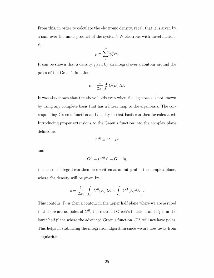
If GR/A is analytic in the upper/lower complex plane respectively, then∮C
GR/A(E)dE =
∫ Emax
Emin
GR/A(E)dE +
∫Γ
GR/A(E)dΓ = 0, (3.17)
where the above holds for any closed path Γ lying in the upper/lower com-
plex planes where GR/A are analytic and once again invokes Cauchy-Gorsat
20

−1.1 0 1.1−1.1
0
1.1
Γ2
Γ1
Figure 3–1: The poles for GR lie in the lower half plane and are enclosed bythe contour Γ2 whereas the poles for GA lie in the upper half complex planeand are enclosed by Γ1.
theorem. Therefore∫ Emax
Emin
GR/A(E)dE = −∫
Γ
GR/A(E)dΓ. (3.18)
Thus, Equation 3.18 gives the result that choosing a contour, Γ in the domain
where the respective Green’s functions are analytic, will allow the computation
of the integral over the real axis.
3.4 General Formalism
Hermitian matrices are normal. Normal matrices can be diagonalized, i.e.
a unitary matrix, X, containing eigenvectors, xi as columns and a matrix, Λ,
containing the associated eigenvalues, λi on the diagonals, can be found such
that
A = XΛX∗. (3.19)
21

Let Xi be a unitary matrix formed by i columns of X where
X∗iXi = Ii.
The eigenprojection, Pi, associated with the eigenvalues, λi, of a matrix A
can be defined by
Pi = XiX∗i
and the matrix diagonalization scheme as in Equation 3.19, can now be written
in terms of a matrix projection as
A =∑i
λiPi. (3.20)
It can now also be shown that the eigenprojection is given by the residues
of the resolvent, R(A, z) = (A − zI)−1, as shown in Equation 3.21 over the
simple, closed contour Γ which encloses the singularities of the resolvent [2]
P = − 1
2πi
∮Γ
R(A, z)dz. (3.21)
Proof. Proof of Equation 3.21
This is a special case of the proof for the contour integral shown in Equa-
tion 3.21. For the general case, see [2]. Let the algebraic multiplicity, the
number of repetitions of a certain eigenvalue λi, be mi, and the number of
distinct eigenvalues of a matrix A be d. To start off, recall that the resolvent
set of A, z ∈ res(A), is a set of all points for which (A− zI)−1 exists. Let Xi
be a matrix which is formed by mi column vectors associated with a specific
eigenvalue, λi. Also, defining a projection Pi onto the eigenspace associated
with λi, as
Pi = XiX∗i ,
22

then by the spectral theorem, the Hermitian matrix A can be decomposed into
A =d∑i
λiPi.
Recalling that if
A = XDX∗
where D = diagλ, then
A−1 = XD−1X∗
and also for a complex number, z
(A− zI)−1 = X(D − zI)−1X∗.
Thus, Pi as defined above, is also a spectral projection of (A − zI)−1 with
eigenvalues given by
λi = (λi − z)−1. (3.22)
Using Equation 3.22, the spectral decomposition of the resolvent, R(A, z), is
given by Equation 3.23
(A− zI)−1 =d∑i=1
1
λi − zPi (3.23)
Let Ck be a simple closed contour which isolates λk, then by the residue
theorem there are two cases such that
∮Ck
1
λi − z=
−2πi ⇐⇒ i = k
0 else.
(3.24)
Then,
− 1
2πi
∮Ck
(A− zI)−1dz = Pk (3.25)
23

In our case, the Green’s function, G, can be thought of as a resolvent
of the Hamiltonian operator H and the density, ρ, as the projection onto the
eigenspace of the operator.
3.5 Approximations
For the purposes of our work, the specific form of the Hamiltonian will not
be of concern. The only thing to note will be that since electronic configura-
tions and systems have many forces and therefore many energy contributions,
the form of the Hamiltonian will not usually be exact. That means there is
no guarantee of having ”nice” eigenvalues, or in other words, it might not be
diagonalizable. This is where the resolvent formalism becomes useful.
In the system particular to the density functional theory and the Kohn-
Sham formulation, the Hamiltonian is actually a function of the density. Since
the real density of the system is not known until the eigenstates are computed,
the Hamiltonian cannot be written down in the basis of eigenfunctions from the
start (chicken or egg scenario). Instead, it is written down in an approximate
basis and then refined with each iteration of a self-consistent loop until some
criteria is met. This can be viewed as a fixed point method.
How to compute a Hamiltonian given a density of the system is known.
That means given any guess for this density, the Hamiltonian can be written
down in that basis. This is where the matrix representation of the operator
will be used since it is easier to visualize.
3.6 Summary
This section has outlined how to go between the Hamiltonian, to the
computation of electronic density. This is done by the Green’s functional
approach. Since this will be used further, it is most useful to write the Green’s
function in matrix notation as
[ES −H]G = I.
24
From this, in order to calculate the electronic density, recall that it is given by
a sum over the inner product of the system’s N electrons with wavefunctions
ψi,
ρ =N∑i
ψ∗iψi.
It can be shown that a density given by an integral over a contour around the
poles of the Green’s function
ρ =1
2πi
∮G(E)dE.
It was also shown that the above holds even when the eigenbasis is not known
by using any complete basis that has a linear map to the eigenbasis. The cor-
responding Green’s function and density in that basis can then be calculated.
Introducing proper extensions to the Green’s function into the complex plane
defined as
GR = G− iη
and
GA = (GR)∗ = G+ iη,
the contour integral can then be rewritten as an integral in the complex plane,
where the density will be given by
ρ =1
2πi
[∫Γ1
GR(E)dE −∫
Γ2
GA(E)dE
].
This contour, Γ1 is then a contour in the upper half plane where we are assured
that there are no poles of GR, the retarded Green’s function, and Γ2 is in the
lower half plane where the advanced Green’s function, GA, will not have poles.
This helps in stabilizing the integration algorithm since we are now away from
singularities.
25

CHAPTER 4Two Probe Device
4.1 Overview
Thus far, we know how to write down a Hamiltonian in terms of electronic
density in some given basis. We also know how to calculate a density given
a Hamiltonian via a Green’s functional approach. However, we have yet to
discuss what the devices are for which we are interested in calculating the
electronic density. The device of interest in our case, is the two probe device.
By considering interactions in different regions of the device, a Green’s function
in the form of a sparse matrix arises [19]. These two probe devices can be used
for circuitry as gate switches and molecular wires, [3]. Due to their usefulness,
they are discussed in detail in this chapter with an explicit derivation for
the form for a Green’s function motivated by Bloch theorem [14], [16], and a
recursive approach as seen in [24], [7], and [4]. The difference from that work,
will be that in our case, these Green’s functional calculations are done for a
device where the boundary conditions for the bulk potential are known as in
[19]. Doing this, will complete the picture of how to compute the electronic
density for two probe nano-device.
4.2 Infinite System
Suppose that we have the system that consists of atoms as shown in Figure
4–1. There is a molecule in the center (in this case C60, but could be others)
that connects on the left and right to some bulk material. This bulk material,
usually a metal, extends to infinity on either side and will be referred to as
the left and right lead. The region of interest will be the molecule with a
finite part of the bulk material on the left and on the right. For a schematic
26

Figure 4–1: A diagram of a two probe device representing the atoms and theirarrangement.
Figure 4–2: A schematic diagram of the different regions which represent adevice with two leads of infinite length labelled LL and RR.
diagram of the region of interest, see Figure 4–2 and the sections CL, CC and
CR. The left and right infinite leads are labelled by LL and RR respectively.
The full matrix for the Hamiltonian represented here as HFull, will consist
of submatrices representing the different regions in the device. If only the
neighbouring regions interact, the it will have the tridiagonal form. Following
the convention from Figure 4–2, the full matrix will lead to the expression as
HFull =
HLL HLC 0
HCL HCC HCR
0 HRC HRR
. (4.1)
The matrices describing the interaction with the leads are HCL and HCR and
since the device is symmetric, H∗LC = HCL and H∗RC = HCR.
27

Working in the orthonormal (S ≡ I), then the matrix equation for the
full Green’s function GFull is of the form
(EFull −HFull)GFull = I,
and in the expanded matrix notation, it is shown by Equation 4.2 as
EFull −HLL HLC 0
HCL EFull −HCC HCR
0 HRC EFull −HRR
GLL GLC GLR
GCL GCC GCR
GRL GRC GRR
=
I 0 0
0 I 0
0 0 I
.(4.2)
The properties of interest are associated with the central device, so that
the only Green’s function needed is GCC . It can be calculated from only three
equations listed below
(EFull −HLL)GLC = 0, (4.3)
HCLGLC + (EFull −HCC)GCC +HCRGRC = 0, (4.4)
(EFull −HRR)GRC = 0. (4.5)
Solving for GRC and GLC using Equation 4.3 and 4.5 respectively and substi-
tuing into Equation 4.4, GCC is obtained
(EFull −HCC − ΣRR − ΣLL)GCC = I, (4.6)
where the definitions for ΣLL and ΣRR which are referred to as self-energies
of the left and right lead respectively, are given by
ΣLL = HCL[Efull −HLL]−1HLC , (4.7)
28

ΣRR = HCR[Efull −HRR]−1HRC . (4.8)
The effect of the leads can be seen as adding an extra energy contribution
to the overall Hamiltonian. Representing H = HCC+Σ where Σ = ΣRR+ΣLL,
then the effective Hamiltonian, H can once again be represented in a diagonal
form with shifted eigenvalues as written in Equation 4.9 [15]
Hψi = εiψi. (4.9)
4.3 Non-Equilibrium Eigenvalues
Now that we have described the Green’s function for the device of interest
which contains left and right infinite leads, an expression for density can be
written in the case where the leads affect the central device. Recall that
the effects of the leads is essentially an addition of an extra term, Σ to the
Hamitonian, H. In order to calculate the projection onto the eigenbasis, a
similar procedure as in the equilibrium case without the leads can be followed.
Defining a retarded Green’s function, GR to be
[ES −H − ΣR]GR = I, (4.10)
and its complex conjugate, the advanced Green’s function, GA, to be
[ES −H − ΣA]GA = I, (4.11)
with (ΣA)∗ = ΣR.
The electronic density can be calculated from the spectral function, A,
which is defined as
A = i(GR −GA).
29

Note that A can be re-written
A = i(GR(GA)−1GA − GR(GR)−1GA).
Grouping terms, get
A = iGR((GA)−1 − (GR)−1)GA.
Rewriting Equations 4.10 and 4.11 as
ES −H − ΣR = (GR)−1, (4.12)
ES −H − ΣA = (GA)−1, (4.13)
and then subtracting Equation 4.12 from Equation 4.13, we obtain
ΣR − ΣA = (GA)−1 − (GR)−1 = −iΓ,
where we introduced a new variable, Γ, which represents the different in the
energies between the leads [3]. The spectral function now becomes
A = GRΓGA ≡ −iG<.
In this case, G< is the Green’s function for an injection of charge. From this,
the density of states can be defined as
ρ =1
2π
∮G<(E)dE,
where the integral only has poles on the real line as shown before. It can be
computed by using Cauchy-Gorsat theorem and integrating along a path in the
complex plane as done for the equilibrium case when there are no semi-infinite
leads as in Chapter 3.
30

Figure 4–3: This figure represents the allowable energy states for a samplecrystal. The diagram on the left shows the energy bands for particular pointsin Fourier space and the diagram on the right shows where these points arelocated in a crystal lattice.
4.4 Total Density
4.4.1 Fermi Distribution
To better understand what the eigenstates of the Hamiltonian represent,
it is important to know the concept of Fermi-Dirac statistics. A solid can
be described in terms of the allowed and forbidden energy levels, or energy
bands that its electrons can be in. This band structure is due to the wave-
like behaviour of electrons which diffract from the crystal lattice structure of
a solid. It defines a solid’s electronic and optical properties and is shown on
the left in Figure 4–3 that depicts the bands of energy (in eV) as different
lines that depend on the position in the solid with positions labelled as Greek
letters on the x-axis. These positions are wave vectors (that is, they are Fourier
transforms of real space variables) and are shown for a simple crystal on the
right of the figure. Statistically speaking, the energy bands of a solid at a given
temperature are filled according to the Fermi-Dirac distribution. This gives a
way to average the behaviour of electrons to get an idea of the macroscopic
properties [14], [11].
31

4.4.2 Fermi-Dirac Statistics
Fermi-Dirac distributions are used to describe fermions (or particles with
half integer spin) such as electrons, (spin 1/2), that obey the Pauli exclusion
principle. It states that no more than one electron can exist in a specific
energy configuration or quantum state. The Fermi-Dirac distribution, labelled
as f(εi), describes the probability of state i with energy εi is
f(εi) =1
e(εi−µ)/kT + 1. (4.14)
Here, the chemical potential is µ, the temperature T and k is the Boltzmann
constant. The statistical distribution is valid only if the number of fermions
in the system is large enough so that the chemical potential µ does not change
if more electrons are added to the system. At temperature, T = 0 and for
energies less than the Fermi energy, all the states are occupied, f(εi) = 1,
while for energies greater than the Fermi energy, there are no electrons in those
states, f(εi) = 0.
The notion of an electronic chemical potential, Equation 4.15, is also
important. It is the functional derivative of the density functional with respect
to the electron density
µ(r) =
[δE[ρ]
δρ(r)
]ρ=ρref
. (4.15)
Considering the particular form of the energy functional, the chemical poten-
tial is effectively the electrostatic potential experienced by the negative charges
present in the system. At the ground state density, the chemical potential is
constant and the electron density is at a steady state so the forces are all
balanced. The use of a chemical potential will become more evident when
examining the device with semi-infinite leads that we are interested in.
32

There are three categories of solids which can be identified based on their
energy band structure. These are classified according to the location of the
valence band and conduction band. The valence band represents the highest
ranges of energy at the zero temperature, which can be occupied by electrons
without being ejected. In organic compounds, this is equivalent to highest
occupied molecular orbital. This concept is equivalent to finding all bound
eigenstates of a Hamiltonian below the Fermi energy. On the other hand, the
conduction band, or the lowest unoccupied molecular orbital is the
lowest energy level that free electrons can achieve which is above the Fermi-
level. For inorganic compounds, the different energy levels are illustrated in
Figure 4–4. Three types of inorganic solids can be identified
1. Metals: where the conduction band and valence band overlap.
2. Semi-conductors: where the conduction band and valence bands are sep-
arated by a small gap.
3. Insulators: where the conduction band and valence bands are separated
by a large gap which is rarely traversed so that electrons cannot be
ejected from the material and therefore the material cannot have induced
current.
Having this knowledge, the full computation for an electronic density will
now require the idea of the Fermi energy and chemical potential. Recall that
ρneq =
∮C
G<(E)dE (4.16)
where now, the energy for left and right leads will incorporate the Fermi-Dirac
distribution
G<(E) = GRΣ<[fLL(E), fRR(E)]GA (4.17)
33

Figure 4–4: This figure illustrates that depending on where the Fermi-energylevel is, the inorganic material will have different properties.
with
Σ<[fLL(E), fRR(E)] = −2iIm[fLLΣLL + fRRΣRR].
The Fermi distribution function, f(E) and it’s representation will not be dis-
cussed in great detail and mentioned for completeness. For a reference, see
[19] or [20].
4.5 Self-Energies
in this section, we will outline how to compute the contributions to the
Hamiltonian which arise from the semi-infinite leads. At first, the discussion
will outline how to compute a Green’s function, also known as the fundamental
solution, for an infinite domain. We then show how to construct the Green’s
function for the semi-infinite domain. We derive a series representation for
the Green’s function for the semi-infinite leads.. This will be done in order to
write a closed form for the Green’s function of the central region.
4.5.1 Inverse of Block Tridiagonal Matrix
We will show a derivation for a formula for computing the inverse of a
tridiagonal matrix using a recursion relation. We start from an example from
34

[7]. Suppose we are interested in solving for Gfull in
HfullGfull = I,
where Hfull is a block tridiagonal matrix. Moreover, let the blocks satisfy
Hij = H∗ji, then
H11 H12 0 0
H∗12 H22 H23 0
0 H∗23 H33 H34
0 0 H∗34 H44
G11 G12 G13 G14
G21 G22 G23 G24
G31 G32 G33 G34
G41 G42 G43 G44
=
I 0 0 0
0 I 0 0
0 0 I 0
0 0 0 I
. (4.18)
Equation 4.18 represents a system of linear equations, four of which are shown
in Equation 4.19.
H11G11 + H12G21 = I
H∗12G11 + H22G21 + H23G31 = 0
H∗23G21 + H33G31 + H34G41 = 0
H∗34G31 + H44G41 = 0. (4.19)
Introducing γ, a matrix defined by
γ+4 = 0
γ+3 = H34[H44 − γ+
4 ]−1H∗34
γ+2 = H23[H33 − γ+
3 ]−1H∗23
γ+1 = H12[H22 − γ+
2 ]−1H∗12, (4.20)
35
γ−1 = 0
γ−2 = H∗12[H11 − γ−1 ]−1H12
γ−3 = H∗23[H22 − γ−2 ]−1H23
γ−4 = H∗34[H33 − γ−3 ]−1H34. (4.21)
Solving the systems of equations in Equation 4.19 as follows,
G41 =− [H44 − γ+4 ]−1H∗34G31
G31 =− [H33 − γ+3 ]−1H∗23G21
G21 =− [H22 − γ+2 ]−1H∗12G11
G11 = [H11 − γ+1 − γ−1 ]−1. (4.22)
Notice that the Gij block is defined recursively. Following the logic of a system
with 4 by 4 blocks, the formula for a block tridiagonal matrix of any size can
be derived
Gii = [Hii − γ+i − γ−i ]−1,
Gij =− [Hii − γ+i ]−1H∗i−1,iGi−1,j, ∀ i > j
Gij =− [Hii − γ−i ]−1Hi+1,iGi+1,j, ∀ i < j (4.23)
where
γ+i = Hi,i+1[Hii − γi+1]−1H∗i,i+1 and
γ−i = H∗i−1,i[Hii − γi−1]−1Hi−1,i. (4.24)
The set of Equations 4.23 is a recursive relation which provides the blocks
comprising the full Green’s function, Gfull. It should be noted that γ−i =
(γ+i )∗. Also, in order to solve the above recursive form, a boundary condition
for γ±i should be assigned in order to compute them uniquely. For example,
36

in the system of 4 by 4 matrix blocks, the conditions were set to 0, i.e.
γ+4 = 0 and γ−1 = 0.
From this comes the formula which states the dependence of the Green’s func-
tion at i+ 1 (or i− 1) on the one at i as shown in Equation 4.25
Gi,i = γ+i + γ+
i Gi−1,i−1γ+i
Gi,i = γ−i + γ−i Gi+1,i+1γ−i (4.25)
4.5.2 Inverse of a Hamiltonian for a Periodic Potential
We now consider a bulk, periodic system. The Hamiltonian is a block-
tridiagonal, infinitely sized matrix with repeating rows as shown below
Hfull =
. . .
. . . H∗int H0 Hint 0 0 . . .
. . . 0 H∗int H0 Hint 0 . . .
. . . 0 0 H∗int H0 Hint . . .
. . .
. (4.26)
The above matrix is a simplified form of the general block tridiagonal
matrix considered in section 4.4.1. In other words
Hii = H0, ∀ i = 1, ...,∞
and
Hi,i+1 = H∗i+1,i = Hint, ∀ i = 1, ...,∞.
37

That means the recursive relations outlined in Equation 4.23 and Equa-
tion 4.25 are now simplified to look like
γ+ = H∗int[H0 − γ+]−1Hint
Gi+1,i+1 = γ+ + γ+Gi,iγ+, (4.27)
where it is still important to note that a boundary condition needs to be given
to solve for γ+.
4.5.3 Bloch Theorem
Instead of going about solving the system by introducing the recursive
relations, they can be uncoupled by taking note of the Bloch theorem which is
essentially described by performing a Fourier transform. Note that the matrix
Hfull is a Hermitian matrix. The Schrodinger equation
HfullΨfull = EΨfull,
can also be written in matrix form as shown in Equation 4.28.
. . .
. . . H∗int E −H0 Hint 0 0 . . .
. . . 0 H∗int E −H0 Hint 0 . . .
. . . 0 0 H∗int E −H0 Hint . . .
. . .
...
Ψl−1
Ψl
Ψl+1
...
= 0. (4.28)
Equation 4.28 consists of infinitely many coupled linear systems, one of which
is shown in Equation 4.29
H∗intΨl−1 + (E −H0) Ψl +HintΨl+1 = 0. (4.29)
It would be difficult to solve for eigenstates Ψl, since there are infinitely many
coupled systems, however, the process can be simplified by a convenient ansatz
38
[4]. Assume
Ψl =∑n
einlφn,
then
Ψl−1 =∑n
ein(l−1)φn,
Ψl+1 =∑n
ein(l+1)φn.
We use this to uncouple Equation 4.30 to get
∑n
H∗inte
−in + (E −H0) +Hinteineinlφn = 0. (4.30)
Equation 4.30 is now the eigenvalue problem written in a different basis. For
ease, denote the Hamiltonian in brackets as
Heff (n) = H∗inte−in + (E −H0) +Hinte
in.
As before, we define the Green’s function
Gkl(n) = (eink)∗[H(n)eff ]−1einl. (4.31)
We now need to represent Gkl in the original basis via
G∞kl =∑n
φ∗n(eink)∗[H(n)eff ]−1einlφn (4.32)
Equation 4.32 provides an explicit representation for the periodic infinite sys-
tem. In Equation 4.23, the Green’s function is computed recursively. These
two ideas can be combined to get a closed form for the Green’s function of a
periodic system for a semi-infinite lead which in turn will allow us to have a
closed form for GCC , the Green’s function for the central device.
4.5.4 Boundary Condition
Since we are interested in semi-infinite leads, we know that the Green’s
function must be zero at some z0 which is where the leads starts. In other
39

words, the fundamental solution is known and it is equivalent to the Green’s
function for an infinite matrix. However, the Green’s function for the semi-
infinite leads has to satisfy the zero boundary condition at one end of the lead
where it is connected to the central molecule. Finding this Green’s function,
is similar to the usual techniques in PDEs. Once again working in operator
notation, we are now looking for a function such that it satisfies Equation 4.33.H(z, z′)GLL(z, z′) = δ(z − z′) in Ω
GLL(z, z′) = 0 on ∂Ω,
(4.33)
where Ω is in the region of the full device. That is, we are looking to modify
the fundamental solution derived in Equation 4.32 to make sure that it is zero
on the boundary. In other words, the Green’s function for the left semi-infinite
lead, GLL will look like
GLL(z, z′) = G∞(z, z′)− γLL(z, z0), (4.34)
where γLL needs to be determined.
Using the recursion relation as in Equation 4.27, a Green’s function for the
semi-infinite lead, GLL can be computed from the general form of the Green’s
function for a block tridiagonal matrix, by realizing that the contribution from
the term which is on the boundary has to be zero. Let this term be the n+ 1
term at the boundary, z0, then
γLL(z, z0) =γ(z, z0)G∞n,n(z, z′)γ(z0, z′)
γLL(z, z0) ≡∑nl,nm
φ∗nm(einl(z−z0))∗φ∗nl
[H(nl)eff ]−1φnl
einm(z0−z′)φnm . (4.35)
40

The full Green’s function for a semi-infinite left lead will then be given
by Equation 4.36
GLL(z, z′) =∑nl
φ∗nl(einlz
′)∗[H(nl)eff ]
−1einlzφnl
−∑nl,nm
φ∗nm(einl(z
′−z0))∗φ∗nl[H(nl)eff ]
−1φnleinm(z0−z)φnm . (4.36)
The Green’s function can be verified to satisfy the correct boundary conditions
for the left lead. Let z = z′ = z0 to see that
GLL(z0, z0) =∑nl
φ∗nl(einlz0)∗[H(nl)eff ]
−1einlz0φnl
−∑nl,nm
φ∗nm(einl(z0−z0))∗φ∗nl
[H(nl)eff ]−1φnl
einm(z0−z0)φnm .
Using
φnleinm(z0−z0)φnm = φnl
φnm = δml
where γml is the Kronecker delta. We then arrive at
GLL(z0, z0) ≡ 0
A similar process is used for the right lead [19], [16]. Once we have a closed
form for GRR and GLL, these can now be substituted into Equations 4.7 and
4.8 for ΣLL and ΣRR. In turn, these can now be used to find GCC using
Equation 4.6.
4.6 Spectra
Let X be an operator in a Banach space with elements x and the identity
operator I. The resolvent, R(λ) is defined in Equation 4.37 where λ is a
complex number.
R(λ) = (λI − x)−1 (4.37)
41

The resolvent set is then the set of all λ in the resolvent. The spectrum,
σ(X) is the defined as the set of all λ in the complement of the resolvent set
as shown in Equation 4.38
σ(λ) ≡ C \R(λ) = λ ∈ C | λ /∈ R(λ). (4.38)
as in [5].
The Hamiltonian has a spectrum that can be grouped into three categories
[18]:
1. The point spectrum: the spectrum of the operator, G that consists of
eigenvalues, λ, such that λI − H is not injective, i.e. the set of all the
eigenvalues is the point, or discrete spectrum. The eigenstates associated
with this spectrum correspond to bound states.
2. The continuous spectrum: the set of all numbers λ which are not in
the discrete eigenvalue set and those whose Range(λI −H) is dense.
3. The singular spectrum: the set of λ for which Range(λI −H) is not
dense.
For example, the Schrodinger equation for the hydrogen atom has both
a point and a continuous spectrum. The form of the Hamiltonian for this
particular system is
−∆ψ(r) +c
rψ(r) = λψ(r),
where c is a constant. It can be shown that λn = 1/n for integers n such that
0 < n < N with discrete eigenvalues λN ≤ ... ≤ λ1 ≤ 0. This s referred to
as the discrete spectrum. However, it can be seen that as r → ∞, then the
Schrodinger can be simplified to
−∆ψ(r) = λψ(r).
42

This has the solutions ψ(r) = e−ikr for |k|2 = λ. These solutions are valid for
all λ ∈ [0,∞) and the result is a continuous spectrum.
To emphasize, the point spectrum of a Hamiltonian has associated states
which are bound whereas the continuous spectrum corresponds to free states.
The electrons which contribute to the current in an electronic device, are
those electrons which are allowed to move around the device and thus have a
continuous spectrum. The energy for which bound states become free states,
corresponds to the energy which is above the highest eigenvalue in the point
spectrum of the Hamiltonian. This is eigenvalue is the Fermi energy.
Intuitively, we can now state that the total electron density, ρTOT , is the
sum of the equilibrium and non-equilibrium contributions,
ρTOT = ρeq + ρneq.
The non-equilibrium contribution to the density, ρneq, arises from having a flow
of electrons. If the leads that are part of the device of interest, have potential
difference ∆V , the electrons will flow in the device to try to compensate and
bring the system to equilibrium. This concept introduces natural bounds for
the integral which is used to compute ρneq as shown in Equation 4.39
ρneq =1
2π
∫ Emax
Emin
G<(E)dE, (4.39)
where
Emin = min(µLL + VLL, µRR + VRR) and Emax = max(µLL + VLL, µRR + VRR)
and Emin and Emax correspond to Fermi levels of the right and left leads, RR
and LL. The rest of the contribution to the electronic density comes from the
43

equilibrium density, ρeq where the bounds are set by 0 and Emin [20].
ρeq =1
2πi
∫ Emin
0
GR(E)−GA(E)
dE ≡ − 1
π
∫ Emin
0
Im[GR(E)]dE. (4.40)
4.7 Discussion of Basis Functions
As previously seen in Chapter 3, in order to compute the Green’s function,
a Hamiltonian H, must be written in some complete basis φi
Hij = φ∗iHφj.
These basis functions should ideally be chosen such that the new Hamiltonian,
H, is a sparse matrix. This can be done by choosing those φi as the linear
combination of atomic orbital basis functions (LCAO). These are derived
from solving isolated atom equations and cutting off the functions at some
artificial barrier.
However, there is one problem with writing down the full problem in the
LCAO basis. That comes up when one is trying to compute the contributions
to the Hamiltonian as outlined in Equation 5.3 and solving the Poisson equa-
tion for the Hartree potential, Equation 2.13. The potential has a representa-
tion in the real basis, but the representation for the PDE and the associated
boundary conditions would be unclear in the LCAO basis. That means once
there is a guess for the electronic density, it must be converted from real space
to LCAO basis for the computations of the Green’s function and thus the
electronic density. After this, the form of the potential must be refined by
converting the electronic density to a real space density and then solving the
Hartree contribution to the potential. This is summarized in Equation 4.41
H → ρ→ ρ→ V → V → H. (4.41)
44

where ˜ represents the computations done in the LCAO basis and the ones
without it are the quantitites computed in the real basis, R3.
4.8 Summary
In this chapter, the Green’s function for a two-probe device is now given
in terms of self-energies of the leads, Σ as
GR = [Efull −H − ΣR]−1 = (GA)∗
The Green’s function due to injection of charge, G<, was introduced as
G< = GA −GR.
Also, definitions of the Fermi distributions and chemical potentials which al-
lowed the calculations of Emin and Emax as bounds for the integral used to
compute the non-equilibrum contribution to the density, ρneq where
ρneq =1
2π
∫ Emax
Emin
G<(E)dE.
Using several identities, ρeq can also be calculated as
ρeq = − 1
π
∫ Emin
0
Im[GR(E)]dE.
After this, a closed form for the Green’s function was introduced by the use
of Bloch’s theorem and a recursive formula. This led to the definition seen in
Equation 4.36. Using that form of GLL and a similar form for GRR, these can
be substituted into the block tridiagonal matrix for the Green’s function as
seen in Equation 4.2. From this, the electronic density for the central region,
based on GCC can now be computed.
45

CHAPTER 5Numerical Methods and Results
5.1 Overview
So far, a complete overview of how to model a two probe nano-electronic
device has been laid out. This chapter will discuss how to compute the elec-
tronic density numerically. The method and code to compute electronic den-
sity was formulated by Dr. Hong Guo’s group at McGill university [19], [20]
and is described here. The difficulty of the computation is shown to be the
computation of the Green’s function at different energy values [19] for each it-
eration of the Kohn-Sham scheme. To alleviate this computational bottleneck,
a preconditioning method is presented. This method is based on the iterative
nature of the problem. As it is shown here, successful preconditioning lowers
the condition number. In turn, solving a linear system iteratively as described
in [21], [8], with preconditioning, is shown to lower the number of iterations
required.
5.2 Kohn-Sham Equations
Recall from Chapter 2 that the total energy functional of the system can
be uniquely defined in terms of density as
E[ρ] =
∫Ω
v(x)ρ(x)dx+ T [ρ] + Vext[ρ]. (5.1)
46
Also recall that the density, ρ, is
ρ(x) =N∑i
|ψi(x)|2 with∫R3
ρ(x)dx =N. (5.2)
Thus, the Schrodinger was written as an eigenvalue problem
− ~2
2m∇2ψi(x) + veff (x)ψi(x) = εiψi(x), (5.3)
with veff calculated using
veff (x) = VH [ρ(x)] +δExc[ρ(x)]
δρ(x)+ Vext[ρ(x)]. (5.4)
It should be emphasized that knowing the correct exchange-correlation energy,
EXC , and thus the effective potential, veff , would lead to computing the exact
ground state density. However, since EXC is phenomenologically derived, we
can only ever have approximate ρ.
Equation 5.2 - 5.4 are the Kohn-Sham scheme.We emphasize that ψi and
ρ are interdependent and the Kohn-Sham scheme is a non-linear eigenvalue
problem. It can be solved iteratively, starting with an initial guess for the
electronic density and updating it as shown in the scheme in section 5.2.1.
5.2.1 Schematic of the Solution Scheme
1. Computation of density in LCAO basis via the Green’s functions:
ρTOT = − 1
π
∫ Emin
0
Im[GR(E)]dE +1
2π
∫ Emax
Emin
G<(E)dE
2. Conversion of density into a basis in R3,
ρ = Φ∗ρΦ
47
3. Computation of the potential
V = VH + VXC
from
∇2VH ≡ −4πρ in Ω, subject to VH = Vbulk on ∂Ω
and
VXC = δ
[ρ4/3a1ρ+ a2ρ
2/3 + a3ρ1/3 + a4
b1ρ+ b2ρ2/3 + b3ρ1/3 + b4
]/δρ
4. Conversion of the above potential to LCAO basis
V = C∗V C
5. Finally, computation of H from V .
5.2.2 Bottlenecks
In the scheme outlined, there are two bottlenecks. One of them occurs at
step 1 and the other at step 2 and equivalently step 4. The first calculation
involves a matrix inversion in order to compute G and the other two steps
involve a conversion from one basis to another. This chapter deals with what
can be done to speed up the numerical inversion of the Hamiltonian, H, to
compute the Green’s function, G, in order to avoid that bottleneck.
5.3 Broyden’s Method
Broyden’s method is used to compute the solution to the self-consistent
set of Kohn-Sham equations. This method is a fixed point algorithm and is
sometimes referred to as a generalization of the secant method to a system
of equations from the general category of ”quasi Newton -Raphson” methods.
Broadly, to find a fixed point x for f(x), define a g(x) such that
g(x) ≡ f(x)− x.
48

At a fixed point, g(x) = 0. The derivation of the method starts from expanding
the given function, g(x) as a Taylor series up to the first derivative about x
g(x) ≈ g(x) + g′(x)(x− x) = 0,
and rearranging to find x
x ≈ x− g(x)
g′(x).
This yields to an iterative method. Let x0 be an initial guess, then for k =
0, 1, ..., n,
x(k+1) ≈ x(k) − g(x(k))
g′(x(k)).
In one variable, perhaps the simplest way to approximate the derivative ap-
pearing on the right hand side is to use the secant method. In other words,
we use a finite difference approximation
g′(x(k)) ≈ g(x(k))− g(x(k−1)
x(k) − x(k−1).
Suppose we wish to solve a system of equations, G(x) = 0, where x(k) is a
vector quantity. The derivative in the approximation now becomes a Jacobian,
J(x(k)), leading to Newton’s method
x(k+1) ≈ x(k) − J(x(k))−1G(x(k)). (5.5)
When the system is nonlinear, the Jacobian is relatively costly to compute.
Broyden’s method introduces an approximation to the Jacobian and therefore,
the partial derivatives which appear in the Jacobian as shown in Equation 5.6
Jij(x) =∂Gi
∂xj(x).
49

The Jacobian required to update the initial guess, or J(x(0)) = J (0) can be
computed either analytically, or according to the secant method.
Jij(x(0)) ≈ Gi(x
(0) + ejh)−Gi(x(0))
h, (5.6)
where ej is the unit vector in the j-th direction and h is a small real number.
All the Jacobians for the successive iterates, or J (k), k ≥ 1 will be computed ac-
cording to the ”least-change secant approximation”. Thus, Broyden’s method
becomes
J (k) ≈ J (k−1) − G(x(k) − J (k−1)(x(k) − x(k−1))
||x(k) − x(k−1)||2||x(k) − x(k−1)||T , (5.7)
where ||.|| indicates the L2 norm and T indicates a transpose [17].
For our problem, there is an operator A : ρ → H[ρ] and B : H[ρ] → ρ.
We want to calculate the fixed point of B A.
5.3.1 Convergence
The criteria for terminating the self consistent loop, i.e. the criteria for
determining how good the guess for the electronic density, ρ, depends on
calculating three quantities
1. Density : the difference between the values of electronic density ρ be-
tween different iterations is measured until the L2-norm smaller than
10−3,
||ρ(k−1) − ρ(k)||2 < 10−3.
2. Effective Potential : since the Hamiltonian is dependent on the electronic
density and the electronic density in turn depends on the Hamiltonian,
the difference between different iterates is also measured. Only the ef-
fective potential changes with each iteration, so only the Veff term is of
50

interest. The criteria for its convergence is also 10−3,
||V (k−1)eff − V (k)
eff ||2 < 10−3.
3. Band Structure Energy : Defining EBS ≡ Tr[ρH], the band structure
energy difference between successive iterates can also be compared and
used as a stopping criteria once its below 10−3.
5.4 Gaussian Quadrature
Since the numerical problem at hand is how to speed up the matrix in-
version that occurs when computing the Green’s function
G(E) = [ES −H − Σ]−1,
it is important to mention how many times this matrix inversion occurs. The
function that invokes the computation of G(E) calls the matrix inversion for
each energy, E because
ρ =
∮G(E)dE.
We use Gaussian quadrature to compute the contour integral with a summa-
tion of the function at specific values of E multiplied by a weight, w(Ei) as
shown in Equation 5.8 ∮G(E)dE ≈
∑i
wiG(Ei). (5.8)
5.5 Pseudo-Code
To understand how relevant it is to find a faster way of inverting the
matrices to compute G, it will be shown how frequently these matrices are
1 From now on, for ease, the tilde notation will be dropped. For example,G will now be written as G.
51

called within the numerical algorithm. As shown before, G(Ei) depends on
the Gaussian quadrature points, so it is computed n times. The density, ρ(k) is
then updated using the Broyden’s method which depends on the new Green’s
function and the previously calculated density, F(G(k)(Ei), ρ(k−1)). This is
outlined in Algorithm 1. This will be referred to as the one-dimensional case
since there was no computation which involved the Fourier transforms of the
infinite leads. The number of Gaussian quadrature points examined in this
system is 40.
Algorithm 1 One dimensional system
while convergence is not reached dofor i from 1 to n, the number of quadrature points doG(k)(Ei) = [EiS
(k) −H(k)]−1
end forρ(k) = F(
∑ni=1G
(k)(Ei), ρ(k−1))
k = k + 1end while
The three-dimensional algorithm involves a summation over wavevectors
since Bloch theorem for their computation was invoked. This means there
exists an extra for-loop as shown in Algorithm 2. The number of wavevectors
used in this model is 64. In total, there are then 2560 matrix inversions for
the computation of the electronic density per iteration of the self-consistent
scheme.
Algorithm 2 Three dimensional system
while convergence is not reached dofor j from 1 to number of wavevectors do
for i from 1 to n, the number of quadrature points doG
(k)j (Ei) = [EiS
(k)j −H
(k)j ]−1
end forρ
(k)j = F(
∑ni=1G
(k)j (Ei), ρ
(k−1)j )
end forρ(k) = (
∑mj=1 ρ
(k)j )
k = k + 1end while
52

5.6 Conditioning
Recall that a well-conditioned function f(x), is one with the property
that all small perturbations of the data, x, lead to small changes of f(x). An
ill-conditioned problem is one where small perturbation of x leads to a large
change in f(x). If δx denotes a small perturbation of x and the corresponding
change in the δf where
δf = f(x+ δx)− f(x),
then the absolute condition number κ is defined as
κ = limδ→0sup‖δx‖≤δ‖δf‖‖δx‖
, (5.9)
where the norm ‖.‖ is taken to be the L2 norm for the duration of the chapter,
unless otherwise specified. Similarly, the relative condition number can be
defined as
κ = supδx
(‖δf‖‖f(x)‖
‖x‖‖δx‖
). (5.10)
In the context of linear systems, consider computing
Ax = b.
The relative condition number of the problem will be
κ = ‖A‖ ‖x‖‖Ax‖
(5.11)
Moreover, if A is an invertible matrix, then the condition number of A
satisfies
κ ≤ ‖A‖‖A−1‖ (5.12)
53

Table 5–1: Given energy values, Ei for a sample one-dimensional system.
i Ei
1 −0.000149697867065979 + 0.0173024080601708i2 −0.0983151054208785 + 0.432393745199718i3 −0.734490875450673 + 0.964108347013472i4 −1.63487570292988 + 0.772614290464068i5 −1.98264415420533 + 0.185500582764808i
The notion of conditioning is important in order to see if the Kohn-Sham
scheme is accurate at each step of the algorithm where the guess for electronic
density is refined. Since the density depends on the integral of an inverse of
the Hamiltonian matrix, the condition number for that should be relatively
low so that we know the inverse is well-defined.
5.7 Sample One-Dimensional System
As previously described, the one-dimensional system does not involve
sampling over wavevectors, but does depends on the energy, Ei of the system.
Sample data with 5 given Hamiltonians, these being the 16th, 19th, 22nd, 25th
and 28th iterates of the self-consistent Kohn-Sham scheme, were given. Also
given, were 5 values of E on the complex plane for which the Green’s function
was computed as shown in Table 5–1. The size of the matrices was 696 by 696
with the sparsity pattern can be seen in Figure 5.7.
The methods considered for speeding up the computation of the direct
inverse are the following:
1. Using basic iterative methods
2. Using Krylov subspace methods
3. Preconditioning
A preconditioner was also applied in methods 1 and 2 to speed up their con-
vergence. In testing the algorithms, only the first column of the inverse was
computed.
54

Figure 5–1: The sparsity of the Hamiltonian for a two-probe, one-dimensionaldevice where the size of the matrix is 696 by 696.
5.7.1 Iterative Matrix Inversion Schemes
The current algorithm to invert matrices involved in computations of
electronic properties of the nano-device, uses Matlab’s ”inv” function. This
function is part of a package called ”LAPACK” which has a lengthy user’s
guide and for a summary, the description can be found in [21], so it will not
be outlined here. In this work, alternative methods for finding an inverse were
attempted. These were iterative schemes.The most common include
1. Gauss-Seidel and successive overrelaxation - for matrices that are either
diagonally dominant, or symmetric and positive definite.
2. GMRES - is used for non-Hermitian matrices.
Consider the system
Ax = b,
with A is an n by n complex valued square matrix and x, b ∈ Cn The matrix A
can be split up into an upper triangular matrix U , a lower triangular matrix,
L and a diagonal matrix, D.
A = D + U + L
55
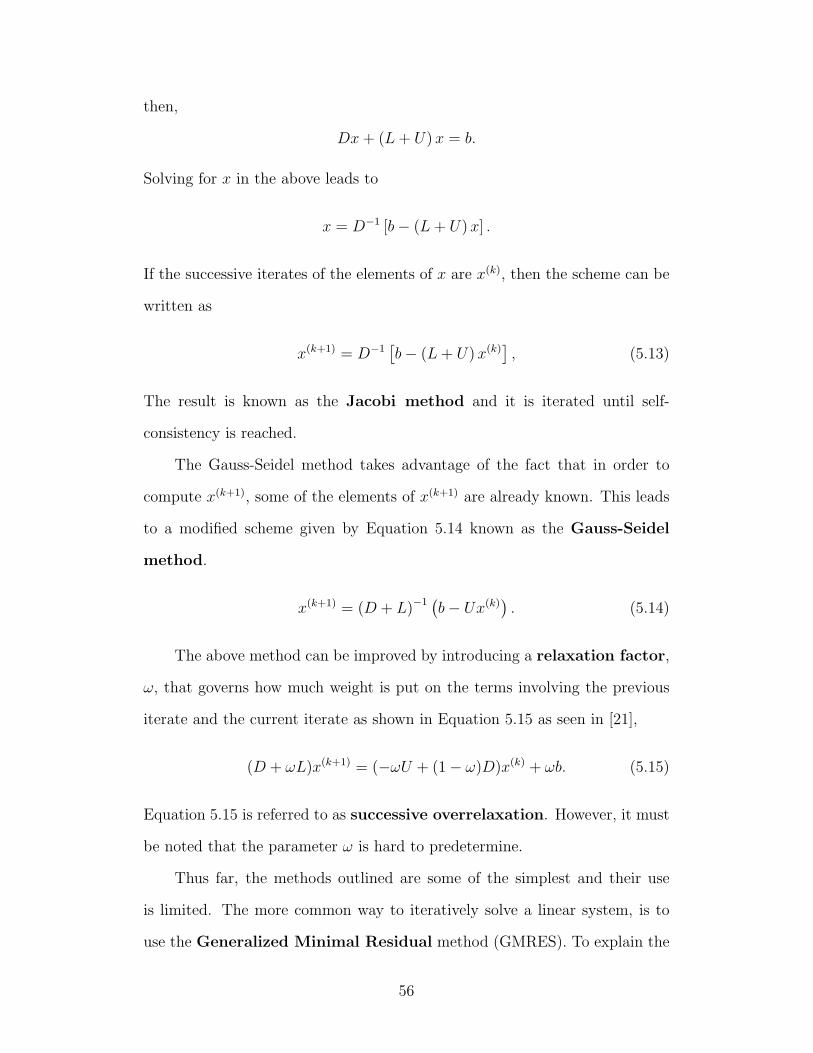
then,
Dx+ (L+ U)x = b.
Solving for x in the above leads to
x = D−1 [b− (L+ U)x] .
If the successive iterates of the elements of x are x(k), then the scheme can be
written as
x(k+1) = D−1[b− (L+ U)x(k)
], (5.13)
The result is known as the Jacobi method and it is iterated until self-
consistency is reached.
The Gauss-Seidel method takes advantage of the fact that in order to
compute x(k+1), some of the elements of x(k+1) are already known. This leads
to a modified scheme given by Equation 5.14 known as the Gauss-Seidel
method.
x(k+1) = (D + L)−1 (b− Ux(k)). (5.14)
The above method can be improved by introducing a relaxation factor,
ω, that governs how much weight is put on the terms involving the previous
iterate and the current iterate as shown in Equation 5.15 as seen in [21],
(D + ωL)x(k+1) = (−ωU + (1− ω)D)x(k) + ωb. (5.15)
Equation 5.15 is referred to as successive overrelaxation. However, it must
be noted that the parameter ω is hard to predetermine.
Thus far, the methods outlined are some of the simplest and their use
is limited. The more common way to iteratively solve a linear system, is to
use the Generalized Minimal Residual method (GMRES). To explain the
56

method, the definition for the residual is needed
r = b− Ax. (5.16)
The idea behind the method is thus minimizing the residual at every itera-
tion. This method is more lengthy to describe, so instead for its derivation,
the book by Trefethen [21] is an excellent resource. Trying out the basic it-
erative methods proved to be successful. Gauss-Seidel converged without a
preconditioner, but in applying a preconditioner, it converged faster. This is
discussed in detail later on. Successive overrelaxation also converged, but the
optimal relaxation parameter is hard to find and in the tests performed, never
improved the convergence rate of Gauss-Seidel, these results are not shown.
5.7.2 Some Notes on Inverses
The criteria for the conjugate gradient method to converge, is that the
matrix is symmetric and positive definite. This is not met by the Hamilto-
nian matrices. MINRES also can’t be applied since the Hamiltonian with
the additions of self-energies is no longer Hermitian. However, the general-
ized minimal residual algorithm, GMRES, does work on the system. We used
GMRES without restarting.
In our case, if we want the full inverse, A−1, this can be computed by
knowing that if b is set to be a vector where only a particular element is 1 and
the rest are zero, for example b = (1, 0, . . . , 0)T ≡ e1, then the resulting x will
be the first column on the inverse. Then if only the second element of b is 1
and the rest are zero, the second column of A−1 is computed. Thus, the full
inverse can be obtained by varying the entries in b. This is derived by using
the fact that
AA−1 = I
57

and letting b be successive columns of the identity matrix. However, some of
the electron transport properties do not rely on the full inverse, but instead
on traces of the inverse (for details, see [3]). Thus, we want to iteratively solve
a linear system
[EiS(k) −H(k)]x(k) = ei (5.17)
with x(k) being a vector we want to compute and ei being a column vector
with only the i-th entry as 1 and the rest zero.
5.7.3 Preconditioning
Suppose we are trying to find a solution, x to the linear system
Ax = b.
If A is ill-conditioned, the inverse will be hard to compute. Introducing now a
matrix, M , also called a preconditioner, and multiplying both sides of the
original equation
M−1Ax = M−1b = c,
would lead to
x = [M−1A]−1c.
If the condition number of M−1A was now lower, then the system would be
faster to solve iteratively. The hard part is finding this matrix M , a pre-
conditioner to lower the condition number without many extra computational
steps.
For the particular system at hand, it is desired to find the Green’s function
for each iteration (k) of the self consistent loop of the Kohn-Sham scheme,
given by
G(k) = (ES −H(k) − Σ)−1. (5.18)
58

Label H(k) = ES−H(k)−Σ where this H(k) is previously calculated. In trying
to calculate the next iterate of the Green’s function, G(k+1), the previous iterate
G(k) can be used to make the matrix have a lower condition number. Since the
self-consistent iteration over the Green’s functions finds an inverse of a matrix
that is similar to the matrix in the previous step, their inverses at each step
(since we are interested in refining the electronic density at each step until
convergence) should also be similar. Thus,
G(k+1)H(k) ≈ I (5.19)
H(k+1)G(k) ≈ I. (5.20)
One method of preconditioning is then
G(k+1) = G(k)(H(k+1)G(k))−1. (5.21)
This means the matrix to be inverted when preconditioned with the previous
iterate’s inverse, will have a lower condition number. For iterative inversion
algorithms which are useful for large sparse matrices, this helps the schemes to
converge faster. Also, if we are only interested in computing specific columns
of the inverse, this will be even faster with an iterative linear solve for x(k) as
in Equation 5.17.
5.7.4 Results
The figures below summarize the number of iterations is takes to solve a
linear system for different preconditioning methods. There are four methods
for each scheme and the dotted line always represents the non-preconditioned
Gauss-Seidel (in red on the upper part of the graphs) and GMRES methods
(in blue on the lower part of the graphs) for comparison. The Gauss-Seidel
algorithm was written by us and Matlab’s ”GMRES” code with and without a
preconditioner was used. The dashed line for GMRES represents what happens
59

when the preconditioner was applied at each iteration of the iterative solver
and the solid line represents inverting a previously preconditioned matrix.
Only computation of the first column of the inverse, x(k) was done, as in
M−1[EiS(k) −H(k)]x(k) = M−1e1.
Tolerance for when the algorithm was assumed to have converged was set to
10−6. It represents the L2 norm of the difference between successive iterates
of the inverses generated by the iterative inverse algorithm
tolerance = ‖x(k−1) − x(k)‖ ≤ 10−6.
The preconditioner varied depending on the method and was always a previ-
ously calculated Green’s function, M−1 ≡ G.
60
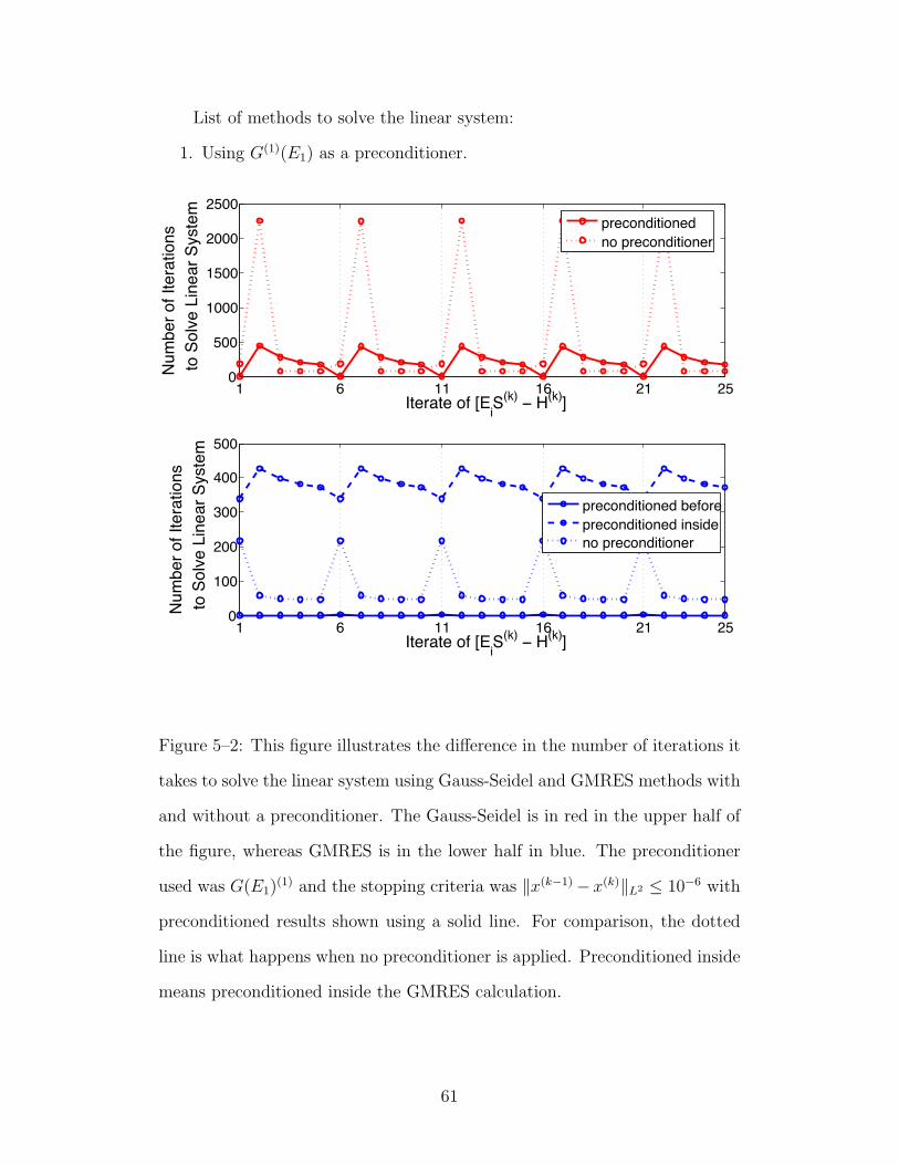
List of methods to solve the linear system:
1. Using G(1)(E1) as a preconditioner.
1 6 11 16 21 250
500
1000
1500
2000
2500
Iterate of [EiS(k) − H(k)]
Num
ber o
f Ite
ratio
ns
to S
olve
Lin
ear S
yste
m
1 6 11 16 21 250
100
200
300
400
500
Iterate of [EiS(k) − H(k)]
Num
ber o
f Ite
ratio
ns
to S
olve
Lin
ear S
yste
m
preconditionedno preconditioner
preconditioned beforepreconditioned insideno preconditioner
Figure 5–2: This figure illustrates the difference in the number of iterations it
takes to solve the linear system using Gauss-Seidel and GMRES methods with
and without a preconditioner. The Gauss-Seidel is in red in the upper half of
the figure, whereas GMRES is in the lower half in blue. The preconditioner
used was G(E1)(1) and the stopping criteria was ‖x(k−1)− x(k)‖L2 ≤ 10−6 with
preconditioned results shown using a solid line. For comparison, the dotted
line is what happens when no preconditioner is applied. Preconditioned inside
means preconditioned inside the GMRES calculation.
61

2. Using G(1)(E2) as a preconditioner.
1 6 11 16 21 250
500
1000
1500
2000
2500
Iterate of [EiS(k) − H(k)]
Num
ber o
f Ite
ratio
ns
to S
olve
Lin
ear S
yste
m
1 6 11 16 21 250
100
200
300
400
500
Iterate of [EiS(k) − H(k)]
Num
ber o
f Ite
ratio
ns
to S
olve
Lin
ear S
yste
m
preconditionedno preconditioner
preconditioned beforepreconditioned insideno preconditioner
Figure 5–3: This figure illustrates the difference in the number of iterations it
takes to solve the linear system using Gauss-Seidel and GMRES methods with
and without a preconditioner. The Gauss-Seidel is in red in the upper half of
the figure, whereas GMRES is in the lower half in blue. The preconditioner
used was G(E2)(1) and the stopping criteria was ‖x(k−1)− x(k)‖L2 ≤ 10−6 with
preconditioned results shown using a solid line. For comparison, the dotted
line is what happens when no preconditioner is applied. Preconditioned inside
means preconditioned inside the GMRES calculation.
62

3. Using G(Ei)(1) as a preconditioner with energy values corresponding to
the same energy as the matrix to be inverted.
1 6 11 16 21 250
500
1000
1500
2000
2500
Iterate of [EiS(k) − H(k)]
Num
ber o
f Ite
ratio
ns
to S
olve
Lin
ear S
yste
m
1 6 11 16 21 250
100
200
300
400
Iterate of [EiS(k) − H(k)]
Num
ber o
f Ite
ratio
ns
to S
olve
Lin
ear S
yste
m
preconditionedno preconditioner
preconditioned beforepreconditioned insideno preconditioner
Figure 5–4: This figure illustrates the difference in the number of iterations it
takes to solve the linear system using Gauss-Seidel and GMRES methods with
and without a preconditioner. The Gauss-Seidel is in red in the upper half of
the figure, whereas GMRES is in the lower half in blue. The preconditioner
used was G(Ei)(1) and the stopping criteria was ‖x(k−1)− x(k)‖L2 ≤ 10−6 with
preconditioned results shown using a solid line. For comparison, the dotted
line is what happens when no preconditioner is applied. Preconditioned inside
means preconditioned inside the GMRES calculation.
63

4. Using the previously computed Green’s function from an iteration of
the self-consistent Kohn-Sham algorithm loop, G(Ei)(k−1) as a precondi-
tioner energy values corresponding to the same energy as the matrix to
be inverted.
1 6 11 16 200
500
1000
1500
2000
2500
Iterate of [EiS(k) − H(k)]
Num
ber o
f Ite
ratio
ns
to S
olve
Lin
ear S
yste
m
1 6 11 16 200
100
200
300
400
Iterate of [EiS(k) − H(k)]
Num
ber o
f Ite
ratio
ns
to S
olve
Lin
ear S
yste
m
preconditionedno preconditioner
preconditioned beforepreconditioned insideno preconditioner
Figure 5–5: This figure illustrates the difference in the number of iterations it
takes to solve the linear system using Gauss-Seidel and GMRES methods with
and without a preconditioner. The Gauss-Seidel is in red in the upper half of
the figure, whereas GMRES is in the lower half in blue. The preconditioner
used was G(Ei)(k−1) and the stopping criteria was ‖x(k−1) − x(k)‖L2 ≤ 10−6
with preconditioned results are shown using a solid line. For comparison, the
dotted line is what happens when no preconditioner is applied. Preconditioned
inside means preconditioned inside the GMRES calculation.
64

The condition numbers for the different methods are shown in Figure 5–6.
It is important to note that the condition numbers for matrices which had no
preconditioning and the matrices where the preconditioner was G(1)(E2) had
the same result. Also, these do not represent an absolute measure of how long
it takes to invert a matrix, however, they gives an indication nevertheless.
1 6 11 16 21 250
20
40
60
80
100
120
Iterate of [EiS(k)− H(k)]
Cond
ition
Num
ber
G(1)(E1)
G(1)(E2)
G(2)(E3)
G(1)(Ei)
G(k−1)(Ei)
no precond.
Figure 5–6: This figure illustrates the different condition numbers of matrices
[EiS(k)−H(k)]. Notice that the most successful preconditioning algorithms are
the ones where the energy values of preconditioners coincide with the energy
values of the iterates of [EiS(k) −H(k)].
Also, the preconditioners G(1)(Ei) and G(k−1)(Ei) produce really small
condition numbers and a new figure to show just how small these numbers
are, is shown in Figure 5–7. This figure shows that preconditioning is most
successful when the preconditioners have the same energy value as the linear
65

system since the energy is the greatest contribution to the condition number.
This is because depending on the energy, we can be closer to the eigenvalues
of the Hamiltonian and therefore closer to poles of the Green’s function. If
we were computing a Green’s function at the pole, the matrix would then be
singular.
1 6 11 16 21 251
1.005
1.01
1.015
1.02
1.025
1.03
1.035
Iterate of [EiS(k) − H(k)]
Cond
ition
Num
ber
G(1)(Ei)
G(k−1)(Ei)
Figure 5–7: This figure illustrates the different condition numbers for the two
most successful preconditioning schemes.
2 In these figures, the vertical dotted lines represent the different iterationsof the self-consisten Kohn-Sham algorithm. The superscript k in H(k) and G(k)
represents the iteration number of the Kohn-Sham loop and corresponds toiterates 6, 11, 16 and 21. In between the dotted lines, the integration variable,Ei, is varied for i = 1, ..., 5.
66

5.8 Comments and Future Directions
It was shown that for a one-dimensional system, different preconditioning
schemes reduce the number of iterations required to solve a linear system
and these can be compared with the known solutions for the example shown.
However, the interesting application of this would be for three-dimensional
systems since in that case, it is not necessarily possible to compute a direct
inverse for the larger matrices. In the appendix, the condition numbers for
these larger systems can be seen. Unfortunately due to lack of computing
power and no sample data, the preconditioning strategies were not tested on
these matrices. This will be a subject for future work.
5.9 Summary
In this section, the numerical computation of the electronic density was
shown. In one-dimension, this is given by Algorithm 1 and in three-dimensions,
this is given by Algorithm 2. Both of these algorithms contain at least one ”for”
loop and a ”while” loop. That means a matrix inversion is done inside at least
two loops and this is time-consuming. Since not all entries of the electronic
density are needed, an iterative linear solver is suggested such as Gauss-Seidel
or GMRES. Successful preconditioners to speed up the iterative solvers are
also suggested such as using G(1)(Ei) and G(k−1)(Ei). This lowers the number
of iterations required to solve the system, speeding up the computation of
electronic density.
67

CHAPTER 6Conclusion
In this thesis, we have outlined the mathematical principles behind elec-
tronic density calculations for two-probe devices. At first, the principles of
density functional theory based on theorems by Hohenberg-Kohn [12], [9] were
explained, which led to the formulation of the problem using the Kohn-Sham
equations [13]. They were shown to have solutions that are iteratively com-
puted by the Green’s functional formalism. Using matrix notation, an explicit
equation for electronic density was derived, which required a contour integra-
tion of the Green’s function [23]. Numerically, this is a time-consuming step
which invokes a matrix inversion for each point on the contour integral. To
speed up the matrix inversion, preconditioning strategies were introduced for
iterative methods such as Gauss-Seidel and GMRES. These were tested on
supplied sample calculations and several iterates of the Kohn-Sham scheme
for a one-dimensional system. The result of the preconditioning strategies can
be summarizes as follows
• The condition number varies greatly depending on the energy, Ei.
• Preconditioning the current iterate, k, of the Hamiltonian, EiS(k)−H(k)
by the Green’s function from a previous, (k − 1) iteration, G(k−1)(Ei),
works to reduce the condition of the matrix [EiS(k) −H(k)]Gk−1(Ei) to
almost unity.
• Preconditioning lowers the number of iterations that a GMRES or Gauss-
Seidel needs to go through to converge.
Using the results of this work can lead to faster algorithms for the calculation
of electron transport. If the end goal is to calculate the electronic density,
68

then classic iterative matrix inversions of preconditioned matrices instead of
the currently used direct inversion currently emplyed [19] is strongly recom-
mended. For larger systems, this method of preconditioning can be coupled
to the already existing block diagonal inversion algorithms as in [15], [4] [24]
and [7] and used on three-dimensional systems. However, as it stands, this is
still a subject of future work.
69

APPENDIX: Condition Numbers for Three-Dimensional System
70

The condition numbers for a sample two-probe system were also exam-
ined. Once again, a plot of quadrature points is included in Figure 6–1. In
total there are 40 points with values ranging from 0 to −2.5 along the real axis
and with imaginary values ranging from 0 to 1.2. Figure 6–2 illustrates the
condition numbers of the Hamiltonian given an energy value, E and a wave
vector, k for the two-probe system. The wave vectors are 64 equally spaced
points on a square grid ranging from values of −3 to 3 on each side. The con-
dition numbers of the Hamiltonian range from 10 to just below 75. They are
seen to depend great only the energy value and the k-point, but not as much
on the iteration of the Kohn-Sham scheme. The line in Figure 6–2 represents
the end of one iteration of the Kohn-Sham scheme while each local lowest
point represents the end of each inner ”for” loop over the energy values (for
details refer to Algorithm 2). The greatest influence on the condition numbers
were the energy values, with the one closest to 0 making the Hamiltonian the
most ill-conditioned. The symmetric nature of the condition numbers due to
the regularity of wave vector sampling points can be seen by examining the
iterate of H near the 1280 value. The condition numbers of the Hamiltonian
about that axis are symmetric. Also, the condition numbers for energy values
away from E = 0 are very similar and can be considered low.
71

Figure 6–1: Chosen Gaussian quadrature points for the integration of thesystem in three dimensions.
Figure 6–2: Condition numbers of a sample two-probe device for each com-puted Hamiltonian. Recall that H is a function of energy value in the complexplane, as well as the wave vector. The line divides two successive iterations ofthe Kohn-Sham schemes.
72
REFERENCES
[1] Inc. 7thWave. Nanotechnology now - current nanotechnology applica-tions. http://www.nanotech-now.com/current-uses.htm, June 2009.
[2] Francoise Chatelin. Eigenvalues of Matrices. John Wiley and Sons, 1993.
[3] Supriyo Datta. Electronic Transport in Mesoscopic Systems, volume 3of Cambrige Studies in Semiconductor Physics and Microelectronic Engi-neering. Cambridge University Press, 1995.
[4] K. S. Dy, Shi-Yu Wu, and T. Spratlin. Exact solution for the resol-vent matrix of a generalized tridiagonal hamitonian. Physical Review B,20(10):4237(7), 1979.
[5] Lawrence C. Evans. Partial Differential Equations, volume 19 of GraduateTexts in Mathematics. American Mathematical Society, 1998.
[6] M. S. Gockenbach. Understanding and Implementing the Finite ElementMethod. SIAM, 2006.
[7] Elena M. Godfrin. A method to compute the inverse of an n-block tridi-agonal quasi-hermitian matrix. Journal of Physics, Condensed Matter,3:7843(5), 1991.
[8] A. Greenbaum. Iterative Methods for Solving Linear Systems, volume 17of Frontiers in Applied Mathematics. SIAM, 1997.
[9] P. Hohenberg and W. Kohn. Inhomogeneous electron gas. Phys. Rev.,136(3B):B864(7), 1964.
[10] Antti-Pekka Juaho, Ned S. Wingreen, and Yigal Meir. Time-dependenttransport in interacting and noninteracting resonant-tunneling systems.Physical Review B, 50(8):5528(17), 1994.
[11] C. Kittel. Introduction to Solid State Physics. John Wiley and Sons, Inc.,2 edition, 1963.
[12] W. Kohn. Nobel lecture: Electronic structure of matter - wave functionsand density functionals. In Reviews of Modern Physics, volume 71, page1253(14), 1999.
[13] W. Kohn and L. J. Sham. Self-consistent equations including exchangeand correlation effects. Physical Review, 140(4A):1133(6), 1965.
73

74
[14] M. P. Marder. Condensed Matter Physics. A Wiley-Interscience Publica-tion, corrected printing edition, 2000.
[15] Magnus Paulsson. One particle negf. unpublished description, March 152002.
[16] S. Sanvito, C. J. Lambert, J. H. Jefferson, and Bratkovsky A. M. Generalgreen’s function formalism for transport calculation with spd hamiltoni-ans and giant magnetoresistance in co- and ni-based magnetic multilayers.Physical Review B, 59:11936, 1999.
[17] G P Srivastava. Broyden’s method for self-consistent field convergence ac-celeration. Journal of Physics A: Mathematical and General, 17(6):317(4),1984.
[18] W. A. Strauss. Partial Differential Equations, An Introduction. JohnWiley and Sons, Inc., 1992.
[19] Jeremy Taylor. Ab-Initio Modeling of Transport in Atomic Scale Devices.PhD thesis, McGill University, 2000.
[20] Jeremy Taylor, Hong Guo, and Jian Wang. Ab initio modeling of quantumtransport properties of molecular electronic devices. Physical Review B,63:245407(13), 2001.
[21] L. N. Trefethen and D. Bau III. Numerical Linear Algebra. SIAM, 1997.
[22] V. S. Vladimirov. Equations of Mathematical Physics, volume 3 of Pureand Applied Mathematics, A Series of Monographs. Marcel Dekker, Inc.,1971. Translated by: Littlewood, A.
[23] A.R. Williams, P.J. Feibelman, and N.D. Lang. Green’s function methodsfor electronic-structure calculations. Physical Review B, 26(10):5433(12),1982.
[24] S. Y. Wu, Cocks J., and Jayanthi C. S. General recursive relation for thecalculation of the local green’s function in the resolvent-matrix approach.Physica Review B, 49(12):7957(7), 1994.
[25] D. A. Wunsch. Complex Variables with Applications. Pearson AddisonWesley, 3 edition, 2004.
[26] M. A. Zagoskin. Quantum Theory of Many-Body Systems, Techniquesand Application. Springer, 1998.