electricity market reform - analysis of policy options - gov.uk
TRANSCRIPT
Version: 1.0 Date: 15/12/10
Electricity Market Reform
Analysis of policy options A report by Redpoint Energy in association with Trilemma UK
December 2010

Electricity Market Reform – Analysis of Policy Options, v1.0, December 2010 2
Version History
Version Date Description Prepared by Approved by
1.0 15/12/2010 Final Nick Screen
Vladimir Parail
Duncan Sinclair
Oliver Rix
Phil Grant
Copyright
Copyright © 2010 Redpoint Energy Ltd.
No part of this document may be reproduced without the prior written permission of Redpoint Energy
Limited.
Disclaimer
While Redpoint Energy Limited considers that the information and opinions given in this work are sound,
all parties must rely upon their own skill and judgement when interpreting or making use of it. In particular
any forecasts, analysis or advice that Redpoint Energy provides may, by necessity, be based on assumptions
with respect to future market events and conditions. While Redpoint Energy Limited believes such
assumptions to be reasonable for purposes of preparing its analysis, actual future outcomes may differ,
perhaps materially, from those predicted or forecasted. Redpoint Energy Limited cannot, and does not,
accept liability for losses suffered, whether direct or consequential, arising out of any reliance on its
analysis.

Electricity Market Reform – Analysis of Policy Options, v1.0, December 2010 3
Contents 1 Executive summary .................................................................................................................................................................................................... 5 2 Introduction .............................................................................................................................................................................................................. 12 2.1 Background ........................................................................................................................................................................................................ 12 2.1.1 History of investment in GB electricity market ............................................................................................................................... 12 2.1.2 Current generation mix .......................................................................................................................................................................... 13 2.1.3 Carbon dioxide (CO2) emissions from the generation sector .................................................................................................... 14 2.1.4 Security of supply ...................................................................................................................................................................................... 14 2.2 Decarbonisation agenda ................................................................................................................................................................................. 16 2.3 Carbon Price Support ..................................................................................................................................................................................... 17 2.4 Electricity Market Reform Project............................................................................................................................................................... 18 2.5 Approach to the analysis ................................................................................................................................................................................ 18 2.6 Conventions ....................................................................................................................................................................................................... 20 2.7 Structure of report .......................................................................................................................................................................................... 20 3 Baseline ....................................................................................................................................................................................................................... 21 3.1 Overview ............................................................................................................................................................................................................ 21 3.2 Baseline assumptions ....................................................................................................................................................................................... 21 3.3 Key Features of the Baseline ......................................................................................................................................................................... 24 4 Options to promote decarbonisation ................................................................................................................................................................ 31 4.1 Overview ............................................................................................................................................................................................................ 31 4.2 Policy options .................................................................................................................................................................................................... 32 4.2.1 Carbon Price Support (£50/t) ............................................................................................................................................................... 32 4.2.2 Premium Payments ................................................................................................................................................................................... 36 4.2.3 Fixed Payments .......................................................................................................................................................................................... 39 4.2.4 Contracts for Difference ........................................................................................................................................................................ 43 4.2.5 Strong Emissions Performance Standard ............................................................................................................................................ 47 4.3 Summary of policy impact on hurdle rates ............................................................................................................................................... 49 4.4 Results of modelling ......................................................................................................................................................................................... 50 4.4.1 Carbon dioxide emissions ...................................................................................................................................................................... 51 4.4.2 Plant mix ...................................................................................................................................................................................................... 52 4.4.3 Electricity prices ........................................................................................................................................................................................ 56 4.4.4 Low-carbon support payments ............................................................................................................................................................. 57 4.4.5 Wholesale energy costs .......................................................................................................................................................................... 59 4.4.6 Plant profitability ....................................................................................................................................................................................... 60 4.4.7 Resource costs .......................................................................................................................................................................................... 62 4.4.8 Security of supply ...................................................................................................................................................................................... 64 4.4.9 Cost benefit analysis of decarbonisation options............................................................................................................................. 65 4.5 Sensitivity analysis ............................................................................................................................................................................................. 67 4.5.1 Overview ..................................................................................................................................................................................................... 67 4.5.2 Commodity price sensitivities ............................................................................................................................................................... 67 4.5.3 Low Gas Sensitivity................................................................................................................................................................................... 69 4.5.4 High Gas Sensitivity .................................................................................................................................................................................. 71 4.5.5 Low Carbon Sensitivity ........................................................................................................................................................................... 73 4.5.6 Low Investor Confidence in Carbon Price Support Sensitivity ................................................................................................... 75 4.6 Key messages ..................................................................................................................................................................................................... 78 4.6.1 Impact of options ...................................................................................................................................................................................... 79 4.6.2 Risks of options ......................................................................................................................................................................................... 80 4.6.3 Implementation issues.............................................................................................................................................................................. 82 4.6.4 Summary ...................................................................................................................................................................................................... 83 5 Options to enhance security of supply .............................................................................................................................................................. 86 5.1 Overview ............................................................................................................................................................................................................ 86 5.2 Capacity Payments for All .............................................................................................................................................................................. 86 5.2.1 Description ................................................................................................................................................................................................. 86 5.2.2 Impact on investment risk ...................................................................................................................................................................... 86 5.2.3 Modelling assumptions ............................................................................................................................................................................. 87 5.2.4 Modelling results ....................................................................................................................................................................................... 89 5.3 Targeted Capacity Tender ............................................................................................................................................................................. 97 5.3.1 Description ................................................................................................................................................................................................. 97 5.3.2 Modelling assumptions ............................................................................................................................................................................. 98 5.3.3 Modelling results ....................................................................................................................................................................................... 98 5.4 Key messages ................................................................................................................................................................................................... 101

Electricity Market Reform – Analysis of Policy Options, v1.0, December 2010 4
5.4.1 Impact of options .................................................................................................................................................................................... 102 5.4.2 Risks of options ....................................................................................................................................................................................... 103 5.4.3 Implementation issues............................................................................................................................................................................ 104 5.4.4 Summary .................................................................................................................................................................................................... 104 6 Combination Packages ......................................................................................................................................................................................... 106 6.1 Packages considered ...................................................................................................................................................................................... 106 6.2 Modelling results ............................................................................................................................................................................................. 107 6.2.1 Plant mix .................................................................................................................................................................................................... 107 6.2.2 Carbon dioxide emissions .................................................................................................................................................................... 108 6.2.3 Security of supply .................................................................................................................................................................................... 110 6.2.4 Electricity prices ...................................................................................................................................................................................... 111 6.2.5 Wholesale energy costs ........................................................................................................................................................................ 112 6.2.6 Cost benefit analysis ............................................................................................................................................................................... 113 6.3 Key messages ................................................................................................................................................................................................... 114 6.3.1 Impact of options .................................................................................................................................................................................... 114 6.3.2 Risk of options ......................................................................................................................................................................................... 115 6.3.3 Implementation issues............................................................................................................................................................................ 115 7 Conclusions ............................................................................................................................................................................................................. 116
Appendices
A Scenario and sensitivity name abbreviations .................................................................................................................................................. 117 C Baseline assumptions ............................................................................................................................................................................................ 124 D Estimating hurdle rates ......................................................................................................................................................................................... 129 E Modelling approach ............................................................................................................................................................................................... 132 F Results metrics ....................................................................................................................................................................................................... 134 G Cost benefit analysis ............................................................................................................................................................................................. 136

Electricity Market Reform – Analysis of Policy Options, v1.0, December 2010 5
1 Executive summary
The need for market reform
There is a growing consensus across political parties and within the industry that reforms to the Great
Britain (GB) electricity market are required in order to deliver the investment needed to replace an aging
generation fleet and achieve ambitious targets for reducing the UK‟s carbon dioxide emissions, while
maintaining secure and affordable supplies for consumers.
Baseline analysis
To demonstrate this, we modelled a „business as usual‟ evolution of the GB generation market under
current policies, with a carbon price rising to £70/t by 2030. This Baseline scenario, based on the Central
assumptions of the Department of Energy and Climate Change (DECC), resulted in a carbon intensity of
around 200 g/kWh in 2030, compared to 452 g/kWh in 20091. Despite a 35% generation market share for
renewables, assumed to be achievable under existing policies2, this is still double the 100 g/kWh previously
recommended by the Committee on Climate Change3 (CCC). Although nuclear stations and plant fitted
with carbon capture and storage (CCS) should be competitive with unabated fossil technologies without
subsidy under Baseline assumptions, the key issue is investors‟ lack of confidence that future carbon prices
will rise to the levels assumed by Government, resulting in a significant lag in development of low-carbon
generation other than renewables.
Analysis of the Baseline scenario also highlighted potential future risks to security of supply towards the
end of this decade and into the next. De-rated capacity margins, while expected to be high in the near
term, could fall below 10% towards the end of the decade, lower than they have been over the last ten
years. There is also the added uncertainty surrounding how the system will operate with much more
renewable plant in the mix. The risks stem from a combination of closures of existing plant (25 GW by
2020 or around 30% of existing capacity), uncertain returns for investors in thermal plant, and the
intermittent nature of wind plant and other types of renewables.
Policy response
The policy response to these challenges should be to strengthen incentives to accelerate investment in low-
carbon generation, to counter uncertainty over the long-term evolution of the current carbon market.
There are three broad approaches for achieving this:
evolution of existing policy, for example extending the premium support which renewables
currently receive under the Renewables Obligation (RO) to all low-carbon generators,
1 Carbon intensity figures are based on direct emissions from generation rather than total life-cycle emissions.
2 With adjustments to support levels through re-banding under the Renewables Obligation as needed.
3 See letter to the Secretary of State for Energy and Climate Change dated 17 June 2010 from Lord Adair Turner, Chair of the Committee on
Climate Change. In its Fourth Carbon Budget report, published on 7 December 2010, the Committee has revised its 2030 generation sector target to 50 g/kWh.

Electricity Market Reform – Analysis of Policy Options, v1.0, December 2010 6
introduction of policies that influence investment behaviour by increasing the anticipated costs
of carbon dioxide emissions, either explicitly through a carbon price floor, or implicitly
through constraining emissions such as through an emissions performance standard, and
introduction of policies that more directly target particular volume objectives, such as targets
for low-carbon generation and/or particular technologies, through the provision of long-term
contracts for low-carbon plant.
In addition, mechanisms should be considered to reduce future risks to security of supply by strengthening
the incentives to provide flexible and back-up capacity on both the supply and demand sides.
DECC asked Redpoint Energy and Trilemma UK to analyse a range of policy options and policy packages
designed to address the challenges identified by the Baseline modelling. We initially analysed five different
options to accelerate investment in low-carbon generation, before considering mechanisms for enhancing
security of supply. Finally, we assessed a range of packages that combined the different options.
Policy options to accelerate decarbonisation
The five different options to accelerate decarbonisation span the range of possible approaches identified
above:
Evolution of existing policy
- Premium Payments for all low-carbon generators
Policies that influence investment behaviour
- Carbon Price Support
- Emissions Performance Standards
Policies that target particular volume/technology objectives
- Fixed Payments for low-carbon generators
- Contracts for Difference for low-carbon generators
The analysis suggests that all five of these options could be designed to achieve an illustrative target carbon
intensity of 100 g/kWh by 2030 under DECC‟s Central assumptions by promoting low-carbon generation
through a combination of lowering investment risk and explicit support for low-carbon technologies.
Generation capital expenditure between 2010 and 2030, which is approximately £75bn on a net present
value basis (2009 real terms)4 under the Baseline, would increase by a further £16 to £24bn under the
policy options assessed. There would be increased costs associated with bringing forward nuclear and CCS
investment, but possible savings in delivering the renewables targets with lower cost finance, and significant
reductions in fuel and carbon costs. Should carbon and gas prices rise strongly in the future, as the current
DECC projections assume, the incremental costs of these policies relative to the Baseline could be
relatively modest, in the range £3.6 to £7.8bn to 2030. The analysis suggests that costs to consumers could
actually be lower than the Baseline under some policy options. For example, under the Contracts for
Difference option, the wholesale cost of electricity (including low-carbon support), which currently
accounts for approximately 40%5 of an average domestic customer‟s bill, could be lower on average over
the period 2010-2030 than under the Baseline. However, this result depends on the ability of Government
4 Capital costs are annuitised based on hurdle rates of investment, and then discounted over the period 2010-2030 using a Government Green
Book discount rate of 3.5% real. All assumptions and results are in 2009 real terms.
5 Source: Ofgem Electricity and Gas Supply Market Report, December 2010

Electricity Market Reform – Analysis of Policy Options, v1.0, December 2010 7
to establish effective mechanisms for setting contract price levels that accurately reflect the costs of the
different low-carbon technologies. In the longer run customers would be better protected from further
rises to carbon and fuel prices.
Although each of the options can be shown to deliver the desired outcome under a certain set of
assumptions, external uncertainties such as fuel and carbon allowance prices will be key factors influencing
the decarbonisation pathway. The level of confidence in a policy delivering the 2030 objectives will be
dependent on its robustness to these external drivers. In addition, credibility that the policy will remain
intact in the long-term will be essential for investor confidence.
The different policies also have different implications in terms of the implementation overhead for
Government and industry players, compatibility with existing arrangements and interconnected markets,
and the speed with which they could be implemented. By extension, each of the policy options therefore
could carry a greater or lesser risk of a near term investment hiatus depending on how the transition is
managed.
Premium Payments
Premium Payments, sometimes referred to as „capacity payments for low-carbon generation‟, could be
implemented either through administered tariffs, or through some form of volume-based auction. By
providing additional support for all low-carbon generators, not just renewables, greater levels of investment
in nuclear and CCS might be expected. However, investors would still be exposed to electricity price risk
in general (driven primarily by fuel and carbon price volatility) and uncertainties surrounding future erosion
in the wholesale electricity price as more generation with low variable costs is added to the system,
bringing down the average short-run marginal price. Hence, investors may be seeking premia sufficient to
meet a higher investment hurdle rate.
A possible variant on the Premium Payments option would be to introduce a low-carbon obligation on
suppliers, either alongside the existing RO or as an extension of it. We have not explored this option
explicitly but conceptually it could be similar to the Premium Payments option since it would provide those
low-carbon technologies to which the obligations relate with an additional revenue stream in addition to
selling their electricity.
Therefore, a possible benefit of this option is that it could be implemented as an extension of current
arrangements, reducing the chance of a hiatus in renewables investment compared to some other options.
The key challenge with it is in setting the correct payment levels given the large uncertainty in technology
costs, and uncertainty in future electricity prices. If premia are set too low there is a risk that
decarbonisation objectives are not met, but if set too high there is a risk of excessive economic rents for
generators and higher costs for consumers.
Carbon Price Support (£50/t)
Carbon Price Support would place a floor under the carbon price for electricity generators and should
reduce investment risk in low-carbon technologies by underpinning the electricity price. Our analysis
suggests that a Carbon Price Support level of £22/t6 implemented in 2013 rising to £50/t in 2020 and £70/t
in 2030 should be sufficient to achieve the illustrative 100 g/kWh decarbonisation target for 2030 under
DECC‟s Central fuel price assumptions, by bringing forward new nuclear investment7. It may also reduce
the level of support required under the RO for new renewables investment, saving consumers money in
6 The minimum cost of emissions for generators, including the underlying EU ETS price where this is lower.
7 Note that under Carbon Price Support (£50/t), RO banding is reduced relative to the Baseline in order to meet the illustrative target of 35% of
generation from renewables by 2030. If the RO banding had been left unchanged from the Baseline, Carbon Price Support would also have encouraged more investment in renewables than there is under the Baseline.

Electricity Market Reform – Analysis of Policy Options, v1.0, December 2010 8
the longer run if carbon prices rise as Government expects. Furthermore, Carbon Price Support would
likely reduce domestic emissions in the near term by encouraging coal to gas switching8.
However, our analysis suggests that the effectiveness of Carbon Price Support in driving low-carbon
investment is dependent on the confidence that investors have that this policy will not be subject to future
change. It may also be less effective if investors are forecasting low future gas prices since low-carbon
generation would be less competitive with gas-fired generation. A further consideration is that as the
system decarbonises, the impact of the Carbon Price Support on the electricity price is likely to diminish,
weakening it as an investment signal. As is the case under Premium Payments, investors are exposed to the
risk of this price erosion.
Given our assumption of a constant increase in Carbon Price Support from 2013 to 2020, this is likely to
increase costs to consumers in the near term by increasing the cost of electricity. High carbon emitting
generators will lose, whereas existing low-carbon generators, such as nuclear and renewables, are likely to
gain. There is also the possibility that it leads to the unintended consequence of greater imports from
connected markets where the carbon price is lower (though the extent of interconnection is currently
relatively small).
A key advantage of Carbon Price Support is that it is compatible with current GB electricity market
arrangements and could be implemented relatively quickly, thus reducing the risk of an investment hiatus.
It also maintains a role for the market in determining the generation mix (although the mix of renewables
investment would still be influenced by the different levels of support available under the RO and sub-5MW
Feed-in Tariff mechanisms).
Emissions Performance Standard
An Emissions Performance Standard (EPS) provides a mechanism for limiting the carbon dioxide emissions
from individual plant or across a generation portfolio. In our analysis, we assume a base „Targeted‟ EPS is in
place as a minimum under all policy packages. This Targeted EPS would be structured as an annual
emissions limit, to be applied to all new coal plant at the station level, to ensure that they are at least
partially fitted with CCS and that there are the necessary incentives to run the CCS units even when
carbon prices are low.
In addition, we have also modelled a Strong EPS applied to all fossil plant from 2018, to assess its
effectiveness in driving deeper decarbonisation without additional policies (other than the RO). To address
security of supply concerns, we have assumed that the Strong EPS is implemented as an annual limit rather
than a rate based limit, allowing plant to remain open but limiting operation to progressively lower load
factors. The Strong EPS would lead to early reductions in emissions, and could drive investment in low-
carbon generation. However, the analysis suggests that this investment may come at the cost of high
electricity prices due to the tight restrictions on the operation of fossil plant.
Sensitivity analysis on the Strong EPS policy demonstrates the difficulty in setting the correct level. There is
also a risk for investors in low-carbon generation that an EPS could be softened in the light of future
security of supply concerns.
Based on the analysis, it appears that a Strong EPS is unlikely to be the most effective mechanism to drive
low-carbon investment as a stand-alone policy, but a Targeted EPS designed as an insurance policy against
low-carbon prices could be effectively combined with other policy options.
8 Under the EU ETS, it would be expected that lower emissions from the GB electricity sector in a given year would be offset by higher emissions
elsewhere within the trading scheme.

Electricity Market Reform – Analysis of Policy Options, v1.0, December 2010 9
Fixed Payments
Under a policy of Fixed Payments, low-carbon generators would be offered long-term fixed price contracts
for the output from their plant, with some form of central agent acting as the counterparty. Contract
prices could be set directly by Government or through an auction process. Fixed Payments could help to
de-risk investments (we estimate that reductions in hurdle rates of up to 1-2% may be possible in some
cases) and hence could both accelerate investment in low-carbon generation and reduce overall costs.
Depending on how the policy is implemented, it would require the Government to take a role in
determining future volume targets for low-carbon generation, possibly with a specific technology mix
including targets for decentralised generation.
Since low-carbon generators are insulated from the electricity market, the policy is more robust to
uncertain fuel and carbon prices and risks to future erosion of the electricity price. This increases
confidence in achieving decarbonisation objectives and offers more stable prices for consumers.
Consumers are exposed however, to any poor decisions surrounding the choice of volume targets (and
technology mix), a risk that investors would normally carry.
A challenge with this option is in establishing the correct price level for payments, with the associated risk
of excessive rents to new low-carbon generators. An administered price approach requires Government
to have a good understanding of the costs of different technologies, where information is not always
transparent. A volume-based auction could address this, but introduces other challenges – making the
auction specific enough that bids can be effectively compared, while ensuring that sufficient players can
participate in order to make it competitive. Careful consideration is also required to ensure that
contracted investments are delivered in a timely and efficient manner.
There would be significant implementation issues associated with this policy, including the establishment of
long-term volume targets, the creation of the necessary contracting agent and the urgent requirement to
implement effective grandfathering arrangements for the RO. Investors would also need time to
understand the commercial implications of the new arrangements. An important function of the purchasing
agent would be to re-sell electricity contracts back into the competitive wholesale market in a manner that
preserves, or possibly promotes, market liquidity, for example through day-ahead auctions. However, as
low-carbon generation increases in the longer run, this has the potential to change significantly the nature
of electricity trading with profound implications for the role and strategies of market participants. For
example, by 2030 around 70% of electricity generated could be administered under Fixed Payments, by
which stage the role of electricity suppliers may have changed fundamentally. With so much electricity
being bought and sold at fixed prices, the key strategic differentiator in terms of cost of supply will be
largely gone, and suppliers may then only be competing on cost to serve and quality of service.
Contracts for Difference
Offering low-carbon generators Contracts for Difference (CfDs) against the electricity price, together with
technology specific premia, could also achieve a high degree of earnings stabilisation. Unlike Fixed
Payments, however, generators would still participate directly in the physical market, with the central agent
purchasing wholesale price „risk‟ rather than power, and as a result they would face some residual level of
market exposure (and hence earnings uncertainty). Depending on the design, this could in turn provide
incentives for forecasting plant availability, scheduling output and (for renewables) siting plant efficiently.
The implementation overhead may be somewhat lower compared to Fixed Payments, although there would
be a number of challenges, in particular determining the correct price levels, establishing robust indices
against which the CfDs can be settled, and managing the credit arrangements. While physical positions
would still be traded bilaterally, the change to the long-term financial exposures of generators would be
similar to Fixed Payments, and could have a similar effect on market dynamics in the longer term.

Electricity Market Reform – Analysis of Policy Options, v1.0, December 2010 10
Capacity mechanisms
The Baseline modelling demonstrated possible future risks to security of supply. The analysis suggests that
policies that promote further decarbonisation could exacerbate the risks, since although they should
stimulate new low-carbon investment, it is likely that this will undercut fossil generators, leading to less
investment in these technologies and/or earlier plant closures. The speed of deployment of low-carbon
generation then becomes critical. Delays would exacerbate any security of supply risk.
The security of supply risk should be reduced where it is possible to stimulate an expansion of demand side
response, enabled by smart meters, other demand side technologies and new pricing propositions
encouraging customers to shift demand.
We have analysed two policies designed to mitigate the risk to security of supply further – a universal
capacity payment mechanism (Capacity Payments for All) and a Targeted Capacity Tender. Either could
increase capacity margins and reduce risks to security of supply but could lead to very different outcomes
in terms of capacity mix and costs to consumers.
The analysis suggests that the main effect of a universal Capacity Payments for All could be to extend the
lifetimes of existing plant, rather than necessarily stimulating investment in new plant. This may leave the
system short of sufficient flexibility to manage the intermittency of renewables and could result in the
unintended consequence of keeping high emitting plant on the system for longer. From an implementation
perspective it is difficult to envisage how a universal capacity mechanism would run alongside the existing
bilateral market and not risk the possibility of windfall gains for generators. It seems more likely that such a
mechanism would be associated with a more radical reform of the current arrangements including the
introduction of a pool-based system or organised electricity exchange requiring some level of mandatory
participation. An additional problem with a global capacity mechanism is that it may create obstacles for
the future integration of the GB market with those elsewhere in Europe unless similar mechanisms are the
norm in other markets.
A Targeted Capacity Tender would be more compatible with existing arrangements and could be
implemented as an insurance policy if required. It would place responsibility on a central body, probably
the System Operator, for delivering a defined security standard, by contracting for a mix of back-up
generation capacity (that would not otherwise have been available) and demand side response that meet
specific requirements for flexibility. The costs to consumers of the Targeted Capacity Tender could be
relatively low. In addition, such a mechanism could be used actively to stimulate investment in new sources
of system flexibility, such as demand response. There is, however, a risk that it displaces private investment
or encourages the planning of earlier closures in order to qualify for the tender, thus increasing the
requirement for tendered capacity, leading to an increasing role for the central body/System Operator.
The way that the tendered capacity is deployed and how it influences imbalance prices would therefore be
a very important design consideration.
Combination packages
We have explored combining Carbon Price Support rising more slowly (reaching £30/t rather than £50/t by
2020) with other decarbonisation options, alongside a Targeted Capacity Tender. Adding Carbon Price
Support (£30/t) to Fixed Payments or Contracts for Difference makes little difference in terms of the
amount of low-carbon investment projected by the model. However, it could have a benefit of enhancing
investor confidence prior to the establishment of the new low-carbon support arrangements, thus reducing
the risk of an investment hiatus. In addition, emissions are reduced in the shorter term by encouraging coal
to gas switching. However, by increasing electricity prices it would lead to higher costs to consumers.

Electricity Market Reform – Analysis of Policy Options, v1.0, December 2010 11
Since investors remain exposed to wholesale prices under the Premium Payments option, introducing
Carbon Price Support (£30/t) has a more direct effect on low-carbon investment in this case. It would
allow the level of premia to be reduced, saving consumers money if carbon prices subsequently rise, and
makes the Premium Payments option more robust to lower outturn carbon prices. It may also support
investments in lower cost low-carbon technologies, such as nuclear, without the need for a premium
payment at all.
Conclusions
The analysis suggests that the societal costs of delivering the required levels of decarbonisation differ
between the options due to the impact on financing, and the extent to which the Government may target
different technology mixes. However, these differences are relatively small, equivalent to about 1% of the
total wholesale cost of electricity between 2010 and 2030. Where the options differ more markedly is in
their impact on customers, their robustness to key uncertainties, the complexity of implementation and
consequences for the electricity market as a whole.
Fixed Payments or Contracts for Difference (in conjunction with a Targeted EPS) could deliver the best
value for customers and be the most robust to long-term uncertainties around fuel and EUA prices. The
key risks with these approaches are that they depend on Government being able to set prices and target
volumes appropriately, and that they represent a significant departure from current arrangements, with
longer term consequences for the operation of the market. They would be more costly and time
consuming to implement, and the transition would have to be effectively managed to minimise a potentially
significant hiatus in near term investments. The inclusion of Carbon Price Support (£30/t) within the
package may mitigate this latter risk to some extent.
The Premium Payments option would involve less implementation complexity but would be less robust to
long-term uncertainties. If this route is adopted, there appear to be advantages in combining it with
Carbon Price Support (£30/t) since this would make it more robust and potentially cheaper for consumers
than either option by itself. Establishing the appropriate level to set premia remains a challenge however,
given the uncertainty in future gas prices.
The Fixed Payment/Contracts for Difference approaches clearly place more reliance on Government
intervention and central management (with a corresponding transfer of risks from investors), relative to the
Premium Payments approaches, which have less impact on the market overall. This choice is likely to be
strongly influenced by the trade off between longer term certainty in the generation mix versus risks
associated with Government decision-making under uncertainty and information asymmetry, disruption to
current market arrangements and near-term investment.
Finally, the risks to security of supply appear material but uncertain and an insurance policy may be needed.
Retaining the option to include a Targeted Capacity Tender within the policy package appears to offer a
cost effective mechanism for achieving this and has the potential to stimulate new sources of flexibility.
However, there are many detailed design challenges that will need to be addressed.

Electricity Market Reform – Analysis of Policy Options, v1.0, December 2010 12
2 Introduction 2.1 Background
2.1.1 History of investment in GB electricity market
Thermal generation
Liberalisation of the GB electricity market was initiated with the passage of the Electricity Act 1989. In the
20 years since, there has been significant investment in new thermal generation capacity. During the 1990s
and early 2000s, this investment primarily took the form of Combined Cycle Gas Turbine (CCGT) plant,
which benefited from relatively low capital costs and an abundant, low-cost source of fuel from the North
Sea as the gas market was opened up to competition. This so-called „dash for gas‟ marked a significant
change from previous decades where investment in thermal plant had been predominantly focused on coal
generation.
Nuclear generation
Under the Central Electricity Generating Board (CEGB) and the South of Scotland Electricity Board (SSEB),
nuclear capacity was commissioned in several phases, starting with Magnox reactors in the 1960s and then
Advanced Gas-Cooled Reactors (AGRs) during the 1970s and 1980s. A further reactor, the Sizewell B
Pressurised Water Reactor (PWR) plant, was completed in 1995. Nuclear output increased during the
1990s due to improved plant performance and the commissioning of Sizewell B, but has since declined with
the retirement of the older Magnox reactors and several of the AGR plant suffering from prolonged
outages.
Nuclear assets were not privatised in the initial round of market liberalisation in GB, but rather remained in
state ownership via Nuclear Electric (the former nuclear division of National Power) and Scottish Nuclear.
In 1996, subsequent to the completion of Sizewell B, the AGR and PWR assets of Nuclear Electric and
Scottish Nuclear were combined and privatised as British Energy, with the Magnox assets remaining in state
ownership as Magnox Electric. No new nuclear plant have been commissioned since that time, although
EDF, which now owns British Energy, has indicated an intention to invest in up to four new plants with the
first operational by 2018. RWE and E.ON have formed a joint venture, Horizon Nuclear Power, with
similar plans. Also, a consortium of Iberdrola, GDF SUEZ and Scottish and Southern Energy has announced
that their joint venture company, NuGeneration, is aiming to develop up to 3.6 GW of new nuclear
capacity.
Renewable generation
At the time of the Electricity Act 1989 a Non-Fossil Fuel Obligation (NFFO) was introduced, and this
remained the primary renewable support scheme until 2002. The NFFO was administered as a series of
competitive tenders, for which renewable energy developers submitted bids specifying the price at which
they would be prepared to develop a project. The Government determined the level of capacity for
different technology bands, and offered contracts to the winning bids. The Public Electricity Supply (PES)
companies were obliged to purchase all NFFO generation offered to them and to pay the contracted price
for this generation. The difference between the contracted price and the wholesale price, which
represented the subsidy to renewable generation, was reimbursed using funds from a Fossil Fuel Levy
raised on customer bills.
Prior to 1990 the only renewable technology of any scale in GB was hydro power, predominantly in
Scotland. The UK's first onshore wind farm was opened in Delabole, Cornwall, in 1991, and consisted of
10 turbines with a capacity of 4 MW. Further wind farm developments followed during the 1990s, along

Electricity Market Reform – Analysis of Policy Options, v1.0, December 2010 13
with the development of landfill gas and other biomass-fired generation. By 2002, total renewable output
stood at around 11 TWh – double the 1990 level, but still a small proportion (just over 3%) of total
electricity supply.
The NFFO was considered to suffer from a number of issues, in particular the problem that a high
proportion of winning bids were not ultimately developed. In April 2002, the NFFO was replaced by the
RO. Eligible renewable generation facilities receive Renewable Obligation Certificates (ROCs) for each
MWh of generation. Electricity suppliers are obliged to buy ROCs corresponding to their share of total
electricity sales. This obligation was set at 3% of sales in 2002/03, increasing to 15.4% by 2015/16. A
supplier that does not obtain sufficient ROCs has to make „buy-out‟ payments (£30/MWh in 2002/3, rising
annually in line with inflation)9.
The original RO provided the same support level irrespective of technology (1 ROC for 1 MWh), leading
to strong investment in the lower cost technologies such as landfill gas, onshore wind and co-firing. In May
2007, the Government published a consultation document10 on the introduction of „banding‟, which would
lead to the issue of different numbers of ROCs per MWh for different types of renewable generation. The
Energy Act 2008 provided the necessary powers to introduce banding and the changes to the RO were
implemented from April 2009.
Since the introduction of the RO there has been a steady increase in the development of renewable
capacity, notably wind, with a number of large onshore and offshore wind farms being commissioned in
recent years. The percentage of output supplied by renewable sources in 2009 was 6.7% – more than
double the 2002 total, but still well short of the level that will be required to meet European Union (EU)
2020 targets on the use of renewable energy11.
2.1.2 Current generation mix
Current installed generation capacity by plant type for GB is shown in Figure 1. CCGTs now represent the
largest share of generation type in capacity terms, at around 37% of the total, with the majority of this
having been brought on stream since 1990. Coal plant retain an approximate 32% share, although a
significant proportion of this is scheduled to close over the next one to two decades in response to EU
Directives on emissions. Renewable generation (including hydro, wind, waste and biomass) accounts for
around 10% of total installed capacity, with over half of that comprising onshore or offshore wind.
9 We have assumed in our modelling that headroom of 10% applies under the RO.
10 Reform of the Renewables Obligation, BERR, May 2007, http://www.berr.gov.uk/files/file39497.pdf
11 The UK‟s target is for 15% of overall energy use to be met from renewable sources. In order to achieve this it is expected that around 30% of
electricity generation will need to be from renewable sources by 2020.

Electricity Market Reform – Analysis of Policy Options, v1.0, December 2010 14
Figure 1 GB generation capacity by type – 201012
2.1.3 Carbon dioxide (CO2) emissions from the generation sector
Based on provisional data, total annual CO2 emissions from the generation sector in 2009 were 186 million
tonnes (Mt). On a unit output basis, emissions averaged 452 g/kWh of electricity generated, down from
496 g /kWh in 200813.
Fossil fuel plant are responsible for the majority of these emissions. On a unit output basis, these plant
emitted 573 g CO2 /kWh generated in 2009. However, there is a significant difference between the
average CO2 emissions intensity of coal-fired generation plant (882 g/kWh) and gas-fired generation plant
(376 g/kWh). This means that total emissions are very sensitive to the relative balance of coal versus gas in
the generation mix, which in turn is driven by the relative prices of the two fuels along with the carbon
price.
To give an idea of the potential impact of gas versus coal switching on overall emissions, if all of the
electricity output produced by CCGT plant in 2009 had been generated from coal instead, there would
have been an increase of around 75 Mt in total CO2 emissions (40% above the 2009 level). Conversely, if
all of the output produced by coal plant in 2009 had instead been generated from CCGTs, there would
have been a reduction in CO2 of around 55 Mt (30% below the 2009 level).
2.1.4 Security of supply
Since market liberalisation margins of available generation capacity over peak demand have generally been
maintained at a stable level. Figure 2 shows three measures of the historic capacity margin between 2002
and 2010:
• outturn peak capacity margin, which shows how much excess capacity was actually
declared available during the half-hour period with the highest demand for a given year,
calculated on a backward-looking basis,
12
Source: Redpoint estimates
13 Source: DECC Statistical Release on Provisional 2009 Greenhouse Gas Emissions, March 2010.
CCGT 37.0%
Coal 32.3%
Nuclear 12.6%
Hydro 1.2%
Pumped storage 3.1%
Wind 6.0%
Biomass 0.5%
Other renewable
2.4%
Waste 0.4% Oil 3.4%
GT 1.3%

Electricity Market Reform – Analysis of Policy Options, v1.0, December 2010 15
• historic forecast de-rated capacity margin, which is based on National Grid‟s Seven Year
Statement (NG SYS) forecasts of peak demand and generation capacity (de-rated based on
expected availability) under an Average Cold Spell (ACS) at the year-ahead stage14, to provide
a historic forward-looking measure of security of supply, and
• historic theoretical de-rated capacity margin, which is calculated in a similar fashion to
the previous measure but with NG‟s forecast of ACS demand replaced with the actual outturn
peak demand. It is thus forward-looking with respect to the likely available capacity at the
system peak in a given year, but backward looking with respect to peak demand.
As can be seen from the chart, while there are fluctuations between years there is no obvious trend in any
of the measures of capacity margin, suggesting a broadly stable supply-demand balance. The historic
forecast de-rated capacity margin, which is the most relevant measure for comparison with the forward
projections of de-rated capacity margin in this study, has typically been in the range of 10-15%. This
measure has consistently been below the historic theoretical margin suggesting that outturn peak demand
has been lower on average than National Grid‟s forecast of ACS demand, with the exception of the cold
winter of 2009/10.
The outturn peak capacity margin has been lower than both of these measures. However, this result is not
unexpected since the outturn margin is calculated based on plant declared available on the day. Since plant
can be declared unavailable for both technical and commercial reasons, it is possible that more capacity
could have been made available had it been needed. The biggest difference between the outturn peak
capacity margin and the historic forecast de-rated capacity margin occurred in 2002, due to unexpectedly
low available capacity during the period of highest demand.
14 To construct the data series, we have taken NG‟s forecasts at the year-ahead stage in each year and applied the same capacity de-rating factors
as used in this study. It should be noted that the NG ACS forecast is prepared on the basis of a 31 March year end under the assumption that the
ACS peak demand occurs in January. The actual system peak is calculated on the basis of normal calendar years.

Electricity Market Reform – Analysis of Policy Options, v1.0, December 2010 16
Figure 2 Measures of GB electricity capacity margin15 – 2002 to 2010
2.2 Decarbonisation agenda
The extent of the challenge of climate change is now widely accepted across political parties in the UK. A
Climate Change Bill was introduced by the UK Government in 2008 to respond to this challenge and
create a legally binding, long-term framework to cut greenhouse gas emissions. This requires the UK to
cut overall greenhouse gas emissions by at least 80% by 2050 relative to 1990 levels and sets out a process
for establishing shorter term emissions limits through five-year „carbon budgets‟ (now fixed out to 2022,
with the CCC due to advise on the 2023-2027 period by the end of 2010)16. Meeting these targets will
mean a radical change in the way the UK produces and consumes energy over the coming decades.
This UK-based legislation is in addition to that introduced at EU level where a package of measures (the
„climate and energy package‟) has been implemented to reduce greenhouse gas emissions, improve energy
efficiency and increase energy produced from renewable sources by 2020. In particular, the requirement
for the UK to produce 15% of energy from renewable sources by 2020 will require a significant change
from the current energy mix.
These new legal requirements have led policy makers to review the existing policy, regulatory and market
framework and to consider where changes might be necessary to deliver the required outcomes. This has
involved a combination of scenario analysis, which seeks to identify what investments might be required,
along with a review of the market and regulatory arrangements, which considers whether the correct
incentives are in place to attract and deliver the necessary investments.
15
Note that prior to 2005 the capacity margins shown in the chart have been calculated using data for the electricity system in England and Wales
only. From 2005 onwards, margins have been calculated based on available data for the entire GB electricity system.
16 Note that the timing of publication of this report was such that it could not be updated for the publication of the CCC 4th Carbon Budget report.
0%
5%
10%
15%
20%
25%
2002 2003 2004 2005 2006 2007 2008 2009 2010
Cap
acit
y m
argi
n
Outturn peak capacity margin
Historic forecast de-rated capacity margin
Historic theoretical de-rated capacity margin
Electricity Market Reform – Analysis of Policy Options, v1.0, December 2010 17
A range of scenario studies have been undertaken by various organisations, including DECC‟s 2050 pathway
analysis17, intended to provide the background for overall policy development. These studies have
highlighted the range of possible future pathways. However, there exists a degree of consensus across
these studies that electrification presents an important option in decarbonising the heat and transport
sectors. This conclusion is based upon the assumption that it will be possible to decarbonise the power
sector using existing technologies and over timescales of a few decades. Indeed, studies undertaken by the
CCC have suggested that power sector CO2 emissions of less than 100g/kWh by 2030 are necessary to
put the UK on the pathway to reach 2050 emissions targets for the economy as a whole.
In parallel with these scenario studies, both DECC and Ofgem have undertaken reviews of the market
arrangements. DECC‟s Energy Market Assessment18 and Ofgem‟s Project Discovery19 both concluded that
significant reform of the electricity market would be necessary to attract the levels of investment necessary
to deliver sufficient reductions in emissions over the next two decades. In addition, these reviews
proposed a range of potential reforms to be considered for implementation.
Following the general election in May 2010, the Conservative and Liberal Democrat parties entered into a
coalition government and produced an agreement20 which set out the policies that they would seek to
implement. This agreement included the intention to introduce a floor to the carbon price, feed-in tariffs
for renewable generators, a security of supply guarantee and an emissions performance standard. This
package of proposals has therefore set the power market reform agenda for the new Government.
2.3 Carbon Price Support
Carbon pricing has been at the centre of the UK and EU policy agenda to tackle climate change since 2005
when the EU Emissions Trading Scheme (EU ETS) was initially implemented. The EU ETS establishes a cap
on overall emissions from a defined group of sectors and the corresponding number of emission permits
are allocated or sold into the market. The market price for these permits therefore sets a cost for carbon
emissions and this carbon price has proved increasingly influential in affecting the way that power stations
generate in addition to creating an important new variable that investors in new power plants must
consider.
However, the future price for carbon arising from the EU ETS is highly uncertain and will not only be
driven by market fundamentals, such as gas price and electricity demand, but will also depend on future
policy decisions by the EU and its Member State Governments. Some investors in new power stations may
therefore consider it necessary to ensure that their investments are robust to a potential collapse in the
carbon price while others might look for a higher return in light of this risk. This has led many observers
to suggest that future carbon price uncertainty is slowing the rate of power sector decarbonisation and
increasing the costs of the transition. The new Government therefore included a proposal to introduce a
carbon price floor as part of the Coalition Agreement.
A carbon price floor can be implemented in various ways. However, so long as it directly affects the costs
of power station emissions, it will constitute an important element of the market arrangements and will
17
Downloaded from http://www.decc.gov.uk/assets/decc/What%20we%20do/A%20low%20carbon%20UK/2050/216-2050-pathways-analysis-
report.pdf
18 Downloaded from http://www.decc.gov.uk/assets/decc/1_20100324143202_e_@@_budget2010energymarket.pdf
19 See http://www.ofgem.gov.uk/Markets/WhlMkts/Discovery/Pages/ProjectDiscovery.aspx
20 „The Coalition: our programme for government‟, http://www.cabinetoffice.gov.uk/media/409088/pfg_coalition.pdf

Electricity Market Reform – Analysis of Policy Options, v1.0, December 2010 18
influence both operational decisions for existing plant and the investment case for new projects. It has
therefore been an important element of the analysis which is described in this report.
Proposals for supporting the carbon price are the subject of a separate stand-alone consultation by HM
Treasury. However, it is important to recognise the interactions between this proposal and the other
elements of market reform.
2.4 Electricity Market Reform Project
The Government initiated the Electricity Market Reform (EMR) project to consider the best way to
implement the proposals contained within the Coalition Agreement. In particular, it was recognised that
the individual elements could be designed a wide variety of ways and that they would interact such that the
outcome would be driven by the overall package rather than the individual elements.
The Electricity Market Reform project has therefore concentrated on identifying the key design options for
implementing feed-in tariffs for renewables, a security of supply guarantee and an emissions performance
standard and assessing how they operate as a package along with a floor to the carbon price.
Redpoint and Trilemma UK were commissioned to undertake a quantitative assessment of the proposed
packages of reform through modelling investor behaviour in the power generation sector out to 2030.
Given the extent of the potential reform options, it has been necessary to supplement the quantitative
work with a qualitative assessment of the proposed reform packages. However, it is important to note
that many detailed design and implementation issues lie outside the scope of this study and remain to be
considered at a later date.
2.5 Approach to the analysis
The focus of the study is a detailed quantitative assessment of the different options for Electricity Market
Reform. We have grouped the analysis into three areas:
options to promote decarbonisation, including Carbon Price Support, Emissions
Performance Standards, and targeted low-carbon support
options to enhance security of supply, including universal capacity mechanisms and
targeted capacity tenders, and
combination packages, which combine some of the above options.
It should be recognised that the analysis requires a large number of assumptions, which are subject to
considerable uncertainty. Hence, the quantitative analysis should be used to inform comparisons between
options but not regarded as a prediction of the future. Given the complexities involved, it has not been
possible to capture every aspect of each policy option within the analytical framework, and we have
therefore supplemented the quantitative analysis of the options with some qualitative assessment.
As a starting point for the analysis we have established a „Baseline‟ for the period 2010 to 2030, which is
intended to represent a Business As Usual case. This is based on current policy, and incorporates DECC‟s
Central assumptions on fuel prices, carbon prices, demand, maximum build rates and capital costs within
Redpoint‟s investment modelling framework. This Baseline is then used as a comparison, or counterfactual,
for the different EMR options.

Electricity Market Reform – Analysis of Policy Options, v1.0, December 2010 19
The objective of the quantitative analysis is to understand better the possible impact of the different EMR
options relative to the Baseline in the following areas:
the pace and extent of decarbonisation
future generation mix
levels of security of supply
overall resource costs, and
costs to consumers.
The analysis is focused on the different financial incentives under each of the EMR options and does not
consider other factors that may affect the rate of new generation investment, such as resource potential,
planning, connections and supply chain constraints. One key assumption, for example, is that these issues
will be sufficiently addressed such that the 2020 renewables target could be met with the right level of
financial support, whether under the Baseline or any of the proposed reform packages.
The EMR policy options to analyse were provided to us by DECC. Our approach to modelling these was
broadly as follows:
identify which of the possible variants of each option to model
qualitatively assess the possible effect of the option on investment risk, and estimate the
impact on cost of capital (hurdle rates)
define policy specific assumptions such as implementation timing and price levels (using
iteration as necessary)
model each option using Redpoint‟s investment modelling framework and compare results
with the Baseline, and
test the sensitivity of the results to key uncertainties.
Within the investment modelling framework is an agent simulation engine which aims to mimic investors‟
decision-making in response to expectations of future revenues relative to the project costs, taking into
account investment risk. Future expectations of electricity prices are formed based on prevailing fuel and
carbon price levels, and forward-looking views of demand and capacity on the system. The supply/demand
balance evolves as investors commit to new build and other plant retire. The model does not assume
perfect foresight, but produces internally consistent results which may reflect cyclicality in returns and
investment patterns.
The model also captures investors‟ forward expectations of revenues under the RO, and new low-carbon
support options required for this study such as Fixed and Premium Payments for low-carbon generators.
We also have enhanced the model to capture the effect of Carbon Price Support and different forms of
emissions performance standard.
The investment decision framework incorporates a simplified dispatch engine to calculate plant output, fuel
usage, carbon dioxide emissions, and to derive electricity prices, at a level of detail appropriate for the
evaluation of multiple policy options. Further details of the modelling framework are provided in Appendix
E.
Electricity Market Reform – Analysis of Policy Options, v1.0, December 2010 20
2.6 Conventions
The main focus of this study has been the Great Britain (GB) electricity market, and our results are
presented on this basis. The generation sector in Northern Ireland is subject to different market
arrangements as a part of the Irish all-island Single Electricity Market (SEM), and separate consideration will
need to be given as to how the policy options considered in this report would be implemented in that
context.
All assumptions and results are in 2009 real monetary terms.
Commodity prices are shown in High Heating Value (HHV) terms.
Unless specifically stated otherwise, the proportion of total generation coming from renewable sources
includes an assumption on the level of renewable microgeneration in each year between 2010 and 2030.
2.7 Structure of report
The remainder of this report is structured as follows:
in Section 3, we present the assumptions and results for the Baseline analysis
in Section 4, we present the analysis of the options to promote decarbonisation
in Section 5, we cover the options to enhance security of supply
in Section 6, we describe and present the results for the combination packages, and
finally, in Section 7, we draw out a summary of the key messages from the study.
In addition we include a number of appendices as follows:
Appendix A contains a glossary of abbreviations of scenario names
Appendix B covers the High Demand Sensitivity
Appendix C sets out additional assumptions and results for the Baseline
Appendix D sets out the methodology for estimating hurdle rates for investment
Appendix E gives a description of our modelling methodology
Appendix F describes our results metrics, and
Appendix G sets out cost benefit analysis results for all packages relative to the Baseline.

Electricity Market Reform – Analysis of Policy Options, v1.0, December 2010 21
3 Baseline
3.1 Overview
The Baseline scenario models the development of the GB generation sector from 2010 to 2030 under
current policy, incorporating DECC‟s Central assumptions on fuel prices, carbon prices, demand, build
rates and capital costs. In this section we summarise the key assumptions behind the Baseline and present
key outputs in terms of generation mix, carbon dioxide emissions and security of supply. These provide
the basis against which we evaluate the EMR policy options, using the Baseline as the counterfactual in our
results analysis. This baseline is consistent with the baseline used in HM Treasury‟s separate consultation
on Carbon Price Support proposals.
3.2 Baseline assumptions
Fuel and carbon prices
For the Baseline, we use fuel price assumptions based on DECC‟s Updated Energy Projections (UEP) June
2010 Central price case. EU Allowance (EUA) carbon price assumptions are taken from DECC‟s Central
assumptions. Further details are provided in Appendix C. All prices are in 2009 real terms.
Taken together, these projections represent a relatively coal favouring environment in the near term21 with
a significant fall in the coal price between 2010 and 2015 before carbon prices start to increase rapidly after
2020.
Demand
The annual demand assumptions for the Baseline correspond to the UEP June 2010 Central scenario for
total electricity supply. In this context, electricity supply is defined as gross generation less the amount of
electricity used on station sites. It therefore corresponds to the term „Supplied (gross)‟ used in the Digest
of United Kingdom Energy Statistics (DUKES) Table 5.6.
Interconnection
We assume a further 1.5 GW of interconnection to the Netherlands and Ireland in 2012, in addition to the
existing French (2 GW) and Northern Irish interconnections (450 MW). Further interconnection is
possible during this period including the possibility of a European Supergrid, but we have not included this
within our Baseline assumptions.
21
As at the time of writing, these assumptions differ from current forward curves. As of 1 Dec 2010, the UK NBP mid-market gas forward price
was 55.0 p/th for Summer 2013 and 61.6 p/th for Winter 2013 (Source: Platts). This compares to an average gas price of 63.3 p/th in 2013 under
DECC‟s Central assumptions. The ARA Coal Year Futures Price for delivery in 2013 as of 1 Dec 2010 was 115 $/t. This compares to an average coal price of 94.1 $/t in 2013 under DECC‟s Central assumptions.

Electricity Market Reform – Analysis of Policy Options, v1.0, December 2010 22
Capital costs
Capital cost assumptions for new build generation have been taken from the Mott MacDonald UK
Electricity Generation Costs Update report, June 201022. These are shown by technology in Appendix C.
Costs are quoted for First Of A Kind (FOAK) and Nth Of A Kind (NOAK) plant, with an assumed switch
date related to expected levels of deployment in GB23. More mature technologies such as CCGTs and
onshore wind are assumed to be NOAK from the start of the modelling time horizon.
Additional learning is assumed to take place on a continuous basis for most technologies leading to further
reductions in capital costs over time. This takes the form of scalar adjustments to capital costs24.
To reflect the fact that there is a spread in project costs, with the best opportunities likely to be exploited
first, a supply curve is modelled which increases capital costs once certain volume thresholds are met by
technology. In addition, there are limits on both annual build rates and total cumulative new build to 2030
by technology25.
Planning and construction
Assumptions on construction and planning times are mostly taken from the Mott MacDonald report. Two
exceptions to this are Offshore Round 1/Round 2 (R1/R2) and Offshore Round 3 (R3) wind plant, for
which the planning times for the purposes of this study are assumed to be two years in both cases. Further
details can be found in Appendix C.
Hurdle rates
Hurdle rates are based on Redpoint assumptions, informed by market data points where possible. We
assume hurdle rates are higher for less mature technologies. Our approach for deriving hurdle rate
assumptions is described in Appendix D.
RO
Under the Baseline, we assume that the RO continues to be the primary mechanism for providing financial
support for large scale renewables (above 5 MW). We assume that it continues until 2037/38, with all
plant guaranteed support until 2027/28 or a maximum of 20 years, whichever is later, subject to the RO
end date. We have adjusted future ROC bands upwards in order to deliver 29% generation from all
renewables by 2020, a figure consistent with DECC‟s Renewable Energy Strategy26 to meet the total 2020
22
Downloaded from http://www.decc.gov.uk/assets/decc/statistics/projections/71-uk-electricity-generation-costs-update-.pdf and adjusted for
DECC exchange rate assumptions where appropriate.
23 Although change from FOAK to NOAK relates to deployment of a given technology in GB, significant deployment of a technology outside of GB
would reduce the difference between FOAK and NOAK costs.
24 Details can be found in Table 1 of Appendix C.
25 Assumptions taken from SKM, Quantification of Constraints on the Growth of UK Renewable Generation Capacity, June 2008
26 See
http://www.decc.gov.uk/assets/decc/What%20we%20do/UK%20energy%20supply/Energy%20mix/Renewable%20energy/Renewable%20Energy%20Strategy/1_20090717120647_e_@@_TheUKRenewableEnergyStrategy2009.pdf

Electricity Market Reform – Analysis of Policy Options, v1.0, December 2010 23
renewables target from domestic production. This outcome assumes that constraints in planning,
connections and the supply chain can be overcome, and that there are sufficient good quality project
development opportunities. ROC bands are subsequently reduced to target an illustrative level provided
by DECC of 35% of generation from renewable sources by 2030. Detailed assumptions on ROC banding
are set out in Appendix C. These changes in to ROC banding are modelling assumptions rather than any
indication of future government banding decisions.
Within the total renewables figures we assume that generation from small scale renewables (sub 5 MW)
under the Feed-in Tariff scheme reaches 2.8 TWh by 2020 before levelling off.
LCPD / IED
The Large Combustion Plant Directive (LCPD) is currently applied to the power sector to limit SOx, NOx
and particulate emissions. This affects the coal and oil fleet in GB. Operators had the option to „opt in‟,
which required them to fit Flue Gas Desulphurisation (FGD) equipment to meet environmental standards,
or „opt out‟, with plant operation limited to a total of 20,000 hours between 2008 and 2015, at which point
they must close. In GB, there are 9 GW of coal plant and 3 GW of oil fired plant that are „opted out‟ and
must close by the end of 2015.
The Industrial Emissions Directive (IED) recasts seven existing Directives, including the Large Combustion
Plant Directive and the Integrated Pollution Prevention and Control (IPPC) Directive, with tighter limits in
particular for NOx emissions, coming into force in 2016. The details of the IED were approved by the
European Parliament during Summer 2010 and have also recently gained European Council approval.
Unlike the LCPD, some older gas plant will also be affected. CCGTs built after 2002, however, are already
compliant. There are four options available to plant which do not meet the NOx limits:
Comply by fitting Selective Catalytic Reduction (SCR) equipment. For gas plant, SCR is not
usually an economic upgrade.
Enter a Limited Lifetime Obligation (LLO). This is analogous to opting out of the LCPD. Plant
can operate up to 17,500 hours over an 8 year period to 2023 and then must close.
Operate under the Transitional National Plan (TNP) as set out by individual Member States.
During the period 2016 – mid-2020 plant will be able to operate as a function of historic
generation levels and have the option of fitting SCR before June 2020 to comply fully.
Enter a Derogation. Under this option, plant will be permitted to run for a maximum of 1,500
hours per year, but with no date for closure. Plant operating under the TNP can opt to enter
a derogation at the end of the TNP in June 2020, but plant operating under the LLO cannot.
The economics of these choices for individual plant are evaluated within the modelling framework.
Nuclear lifetime extensions
Closure dates for existing nuclear plant are based on recommendations by the Nuclear Installations
Inspectorate (NII), which is part of the Health and Safety Executive (HSE). We assume a five year
extension from published closure dates for the three Advanced Gas Reactor (AGR) plant which have not
already been extended. Details of the closure date assumptions for existing nuclear plant are set out in
Appendix C.
It has recently been announced that the Wylfa Magnox nuclear plant will be allowed to operate until 2012
and there is also a possibility that the life of the Oldbury Magnox nuclear plant will be extended beyond the

Electricity Market Reform – Analysis of Policy Options, v1.0, December 2010 24
summer of 2011. Our assumptions for this study were agreed with DECC prior to these announcements,
and the model assumes that both plant are closed by the end of 2010.
CCS demonstration projects
The Baseline assumes that four coal27 carbon capture and storage (CCS) demonstration projects go ahead,
and that sufficient support is provided to enable this. The assumptions for the four projects are shown in
Table 1 below28.
Table 1 Assumptions for CCS demonstration projects
Demo 1 Demo 2 Demo 3 Demo 4
CCS type Post combustion Pre combustion Post combustion Oxyfuel
CCS capacity (MW) 300 360 300 300
Unabated capacity (MW) 1,140 468 1,140 0
Year completed 2014 2015 2018 2018
Under the Baseline (and in all EMR policy runs), CCS is assumed to be a proven technology by 2025.
However, under the Baseline assumptions, none of the unabated units of the demonstration plant would be
retrofitted before 2030 without additional support to cover the costs of the retrofits since investors are
not anticipating the steep increase in carbon prices assumed under the Central assumptions.
3.3 Key Features of the Baseline
Figure 3 shows the cumulative new generation capacity between 2011 and 2030 as projected by the model
under the Baseline assumptions. As explained in Appendix E, the model builds new capacity by simulating
the investment decisions of different agents in the market. Capacity is built where future expected returns
exceed the long-run marginal costs (LRMCs) of different technologies. In forming expectations of future
returns, we assume that investors take a ten year forward view of the expected supply/demand balance, but
use prevailing fuel and carbon prices in their projections of future electricity prices. Hence, the model
assumes that investors do not anticipate future increases in carbon prices, a key factor in determining the
generation mix produced by the model.
Renewables dominate new build with an additional 29 GW added by 2030, of which 17 GW is onshore
wind and 12 GW is offshore wind. New nuclear only comes on-line from 2027 (by which point the carbon
price has reached £54/t), with 6.4 GW added by 2030. There is 11.2 GW of new CCGT coming online
between 2020 and 2025 in anticipation of IED-related retirements.
27
It has recently been announced that the CCS demonstration programme would also be open to gas plant. Our assumptions for the CCS
demonstration plant pre-date this announcement.
28 It is likely that the first demonstration plant will be a retrofit to Scottish Power‟s Longannet plant.

Electricity Market Reform – Analysis of Policy Options, v1.0, December 2010 25
Figure 3 New build – Baseline
Figure 4 shows cumulative retirements between 2010 and 2030 under the Baseline assumptions, broken
down by plant type. During the period between 2010 and 2030, all existing nuclear plant close with the
exception of Sizewell B. Around 12 GW of coal and oil plant retire at the end of the LCPD and a further
11 GW of coal and gas plant by 2023 under the terms of the IED. Further retirements of gas and coal plant
occur on economic grounds throughout the period. By 2030, most existing coal capacity has closed and
that remaining open is co-firing with biomass.
Figure 4 Cumulative plant retirements – Baseline
Figure 5 shows total generation capacity broken down by plant type. Gas represents the largest
component of the overall capacity mix throughout the period between 2010 and 2030. Coal capacity
-
10,000
20,000
30,000
40,000
50,000
60,000
2010 2012 2014 2016 2018 2020 2022 2024 2026 2028 2030
MW
CCGT Unabated Demo Demo CCS
Gas - CCGT with CCS Coal - IGCC with CCS Coal - ASC with FGD & CCS
Nuclear Renewables
0
5000
10000
15000
20000
25000
30000
35000
40000
45000
2010 2012 2014 2016 2018 2020 2022 2024 2026 2028 2030
MW
Oil
GT & OCGT
Nuclear
Coal
CCGT

Electricity Market Reform – Analysis of Policy Options, v1.0, December 2010 26
steadily decreases, being replaced largely by renewables, mainly wind. Nuclear capacity contracts with plant
closures and then expands again as new nuclear plant come on-line from 2027. No new CCS capacity is
developed before 2030 beyond the CCS demonstration plant.
Figure 5 Capacity mix – Baseline
Figure 6 shows total generation broken down by plant type. With gas prices high relative to coal, output
from gas plant declines in the near term but then rises again from 2016 as other plant close under the
LCPD and IED. Likewise, output from coal plant is initially high, but falls off rapidly in the 2020s in
response to a sharply rising carbon price and as a result of plant closures. The output gap left by falling
coal plant output is filled by a mixture of output from renewables and new gas generation.
Output from renewables increases steadily, reaching 29% of electricity generated by 2020, and 35% by
2030, achieved by adjusting ROC bands as described above. Wind accounts for the majority of this output.
The share of biomass in the total generation mix by 2030 is higher than its share of total capacity as it
achieves high load factors relative to wind. This is also the case for nuclear generation, which accounts for
a higher proportion of total generation than of total capacity.
0
20
40
60
80
100
120
GW
GT
Oil
non ROC waste
Other renewables
Biomass
Marine
Wind
Pumped storage
Hydro
Nuclear (new)
Nuclear (existing)
CCS
Coal
Gas

Electricity Market Reform – Analysis of Policy Options, v1.0, December 2010 27
Figure 6 Generation mix – Baseline29
Figure 7 shows total annual carbon dioxide emissions and emissions intensity from the power sector
between 2010 and 2030 for the Baseline. Up until 2023, there is a gradual decline in emissions driven by
the expansion of renewables and the closures of more highly emitting plant (but offset to a degree by
nuclear closures).
After 2024 decarbonisation is more rapid, driven by steeply increasing EUA prices, IED-related closures of
coal plant and the continued expansion of renewable generation. By 2030 the emissions intensity under the
Base Case is around 200 g/kWh, approximately double our assumed decarbonisation target of 100 g/kWh.
Figure 7 Carbon dioxide emissions intensity – Baseline
29
Figures for interconnector represent expected net flows.
0
50
100
150
200
250
300
350
400
TW
h
Interconnector
GT
Oil
non ROC waste
Other renewables
Biomass
Marine
Wind
Pumped storage
Hydro
Nuclear (new)
Nuclear (existing)
CCS
Coal
Gas
0
100
200
300
400
500
600
2010 2012 2014 2016 2018 2020 2022 2024 2026 2028 2030
0
20
40
60
80
100
120
140
160
180
200
CO
2 e
mis
sio
ns
inte
nsi
ty (
g/k
Wh
)
To
tal C
O2
em
issi
on
s (M
t)
Total CO2 emissions (Mt) CO2 emissions intensity (g/kWh)

Electricity Market Reform – Analysis of Policy Options, v1.0, December 2010 28
Figure 8 shows the time-weighted average wholesale price of electricity under the Baseline. It remains
relatively steady until 2015 and then rises on the back of tightening capacity margins in the near term and
rising fuel and carbon prices thereafter. By 2030, the baseload price is approximately double that in 2010
under DECC‟s Central assumptions.
Figure 8 Time-weighted average wholesale price of electricity30 – Baseline
Figure 9 shows the de-rated capacity margins produced by the model under the Baseline assumptions,
compared to historical levels. We also show the non-de-rated margin for comparison, which is simply the
excess of total capacity on the system as a percentage of peak demand. However, with an increasing
proportion of intermittent renewables on the system this becomes an increasingly less reliable indicator of
security of supply.
While recognising the large uncertainty associated with trying to predict future de-rated capacity margins,
these results provide a useful insight into future risks. The years immediately after 2009 are characterised
by a dramatically increasing de-rated capacity margin. This is due to a combination of falling demand as a
consequence of the economic downturn, new CCGT plant coming online and continued renewable new
build supported by the RO. After 2012, capacity margins fall due to the retirement of plant impacted by
the LCPD and IED, together with decommissioning of nuclear plant. After 2018 the de-rated capacity
margin falls below 10%, which is lower than the historical average seen between 2002 and 2010.
These lower capacity margins reflect a changing investment climate. Traditionally, investment in CCGTs
has been on the back of expectations of baseload running, but due to the increasing proportion of
intermittent renewables on the system, CCGTs may only be operating at mid-merit levels. The modelling
suggests that if peak prices can rise to the value of lost load (which we assume to be £10,000/MWh on
average) when the system is very tight, then in theory CCGT investors could earn a reasonable return
operating at lower load factors. However, there is significant uncertainty surrounding this, increasing risk,
and investment may lag as a result. Furthermore, as identified by Ofgem under Project Discovery31, there
are reasons to suggest that under current arrangements prices may not rise high enough to reflect the
value of lost load, thus increasing the security of supply risk further.
30
The term „time-weighted‟ is used to denote a plain average over all hours of a given year.
31 See section 3.26 of http://www.ofgem.gov.uk/Markets/WhlMkts/Discovery/Documents1/Project_Discovery_FebConDoc_FINAL.pdf
2010 2012 2014 2016 2018 2020 2022 2024 2026 2028 2030
0
20
40
60
80
100
120
£/M
Wh
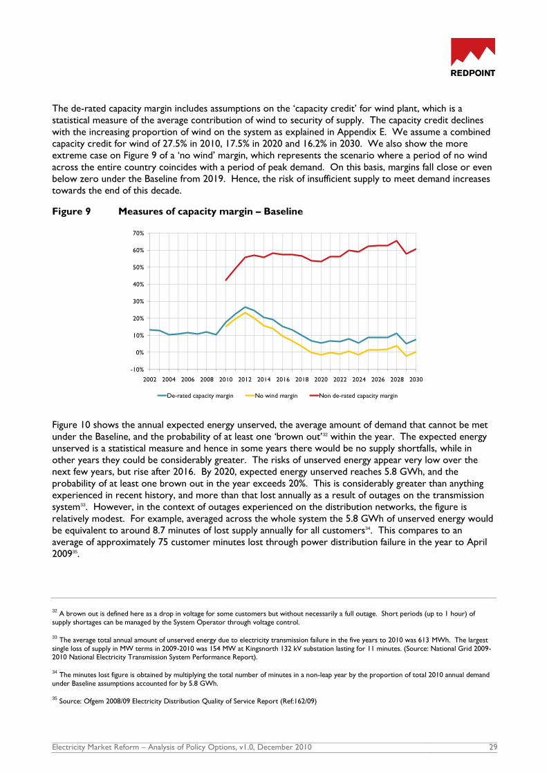
Electricity Market Reform – Analysis of Policy Options, v1.0, December 2010 29
The de-rated capacity margin includes assumptions on the „capacity credit‟ for wind plant, which is a
statistical measure of the average contribution of wind to security of supply. The capacity credit declines
with the increasing proportion of wind on the system as explained in Appendix E. We assume a combined
capacity credit for wind of 27.5% in 2010, 17.5% in 2020 and 16.2% in 2030. We also show the more
extreme case on Figure 9 of a „no wind‟ margin, which represents the scenario where a period of no wind
across the entire country coincides with a period of peak demand. On this basis, margins fall close or even
below zero under the Baseline from 2019. Hence, the risk of insufficient supply to meet demand increases
towards the end of this decade.
Figure 9 Measures of capacity margin – Baseline
Figure 10 shows the annual expected energy unserved, the average amount of demand that cannot be met
under the Baseline, and the probability of at least one „brown out‟32 within the year. The expected energy
unserved is a statistical measure and hence in some years there would be no supply shortfalls, while in
other years they could be considerably greater. The risks of unserved energy appear very low over the
next few years, but rise after 2016. By 2020, expected energy unserved reaches 5.8 GWh, and the
probability of at least one brown out in the year exceeds 20%. This is considerably greater than anything
experienced in recent history, and more than that lost annually as a result of outages on the transmission
system33. However, in the context of outages experienced on the distribution networks, the figure is
relatively modest. For example, averaged across the whole system the 5.8 GWh of unserved energy would
be equivalent to around 8.7 minutes of lost supply annually for all customers34. This compares to an
average of approximately 75 customer minutes lost through power distribution failure in the year to April
200935.
32
A brown out is defined here as a drop in voltage for some customers but without necessarily a full outage. Short periods (up to 1 hour) of
supply shortages can be managed by the System Operator through voltage control.
33 The average total annual amount of unserved energy due to electricity transmission failure in the five years to 2010 was 613 MWh. The largest
single loss of supply in MW terms in 2009-2010 was 154 MW at Kingsnorth 132 kV substation lasting for 11 minutes. (Source: National Grid 2009-2010 National Electricity Transmission System Performance Report).
34 The minutes lost figure is obtained by multiplying the total number of minutes in a non-leap year by the proportion of total 2010 annual demand
under Baseline assumptions accounted for by 5.8 GWh.
35 Source: Ofgem 2008/09 Electricity Distribution Quality of Service Report (Ref:162/09)
2002 2004 2006 2008 2010 2012 2014 2016 2018 2020 2022 2024 2026 2028 2030
-10%
0%
10%
20%
30%
40%
50%
60%
70%
De-rated capacity margin No wind margin Non de-rated capacity margin

Electricity Market Reform – Analysis of Policy Options, v1.0, December 2010 30
Figure 10 Unserved energy and probability of brown out – Baseline
We have made conservative assumptions under the Baseline with respect to the future expansion of
demand side response, only including an estimated 1 GW36 of existing capacity from large scale industrial
and commercial consumers. The roll out of smart and advanced meters to all customers by 2020 could,
for example, help mitigate some of these risks by making demand more responsive to price.
36
Current estimates of demand side response from the I&C sector are taken from Global Insight, May 2005, Estimation of Industrial Buyers'
Potential Demand Response to Short Periods of High Gas and Electricity Prices.
0%
5%
10%
15%
20%
25%
2010 2012 2014 2016 2018 2020 2022 2024 2026 2028 2030
0
1
2
3
4
5
6
7
Pro
bab
ilit
y o
f b
row
n o
ut
(%)
Ave
rage
un
serve
d e
ne
rgy (
GW
h)
Average unserved energy (GWh) Probability of brown out (%)

Electricity Market Reform – Analysis of Policy Options, v1.0, December 2010 31
4 Options to promote decarbonisation 4.1 Overview
Analysis of the Baseline suggests that, assuming current constraints in planning, connections and supply
chains are resolved, and there are enough good quality project development opportunities available, the
RO could provide the financial incentives necessary to deliver a proportion of generation from renewables
sources consistent with the 2020 renewables target. However, it also demonstrates that the carbon
intensity of the electricity system may be well in excess of what is required to meet overall UK carbon
reduction targets, unless greater investment in nuclear and/or CCS occurs. There may also be more cost
effective ways of achieving the renewables targets.
While DECC‟s carbon price assumptions (rising to £70/t by 2030) are „target consistent‟, under our
modelling, investors make no assumptions about future increases in carbon prices, and low-carbon
investment lags as a result. It is also possible that carbon prices turn out lower than DECC‟s Central
assumptions, further jeopardising achievement of the carbon targets.
We have analysed five alternative policy options designed to achieve the following objectives:
29% of generation from renewable sources by 2020
35% of generation from renewable sources by 2030, and
carbon intensity from the electricity system of 100 g/kWh by 2030.
These policy options are:
Carbon Price Support (£50/t)
Premium Payments for low-carbon generation
Fixed Payments for low-carbon generation
Contracts for Difference for low-carbon generation, and
Strong Emissions Performance Standard.
Each of these policies has been designed through iteration to achieve the objectives outlined above under
the commodity prices, carbon prices, demand and technology cost assumptions used in the Baseline. We
test the sensitivity of the results to gas and carbon prices.
There are a range of other options that have not been modelled as a part of this study, in particular a
Regulated Asset Base (RAB) mechanism for new low-carbon generation. This approach would offer a high
degree of certainty to investors, and as such, directionally, could be considered to be similar in impact to
the Fixed Payments option modelled here. The main difference would be that under RAB, investors would
be allowed a certain level of return on their investment for a fixed period, rather than a certain level of
revenue. By lowering the level of risk borne by investors further, this could result in a lower cost of
capital. Different designs could nevertheless leave different levels of risk with generators, such as those
related to construction costs and timeframe, to ensure that appropriate incentives remained in place.
In Section 5, we assess options to address the risks to security of supply highlighted by the Baseline
modelling, and in Section 6 we describe and present the results for a number of combination packages that
incorporate one or more of the decarbonisation options described in this section with capacity
mechanisms described in the next section.
Electricity Market Reform – Analysis of Policy Options, v1.0, December 2010 32
4.2 Policy options
In this section, we describe each policy option, and in particular the way they have been implemented in
our modelling. A key consideration is how each option affects investors‟ risk and what the impact might be
on cost of capital. At this stage it is very difficult to assess what the impact of the EMR policy options could
be in this respect. We have made some assumptions, based on simulating earnings risk under the different
policy options for different technologies using a methodology set out in Appendix D. We recognise that
there is significant uncertainty surrounding these assumptions.
4.2.1 Carbon Price Support (£50/t)
Description
Carbon Price Support places a minimum price on the cost of carbon emitted by generators, thus increasing
confidence in low-carbon investment. By underpinning future carbon prices it should better align
Government and investor future price expectations.
As set out in HM Treasury‟s consultation on Carbon Price Support, it would work by requiring generators
to pay a tax on the fossil fuels they use for power generation based on the carbon content of each fuel.
The levels of tax would be set to target an overall long-term carbon price (EUA price plus carbon price
support tax) for generators.
Impact on investment risk
Table 2 summarises the possible impact of Carbon Price Support on the major sources of investment risk
for five illustrative technologies – CCGTs, nuclear, CCS, wind and biomass. The different types of risk
factors considered, defined as factors posing a potential for downside impact on overall project earnings,
are shown in the left-hand column. The main impact is in reducing risk from low electricity prices
associated with low-carbon prices. Also there is a reduction in load factor risk for CCS and biomass plant,
since there is a lower chance that electricity prices will fall below their short-run generation costs.
Technology risks, such as construction and availability risk, are unchanged.

Electricity Market Reform – Analysis of Policy Options, v1.0, December 2010 33
Table 2 Impact of Carbon Price Support on investment risk
Modelling assumptions
In Appendix D we set out our methodology for estimating the impact of policy options on hurdle rates for
different investments. Based on the results of simulating the earnings risk for different types of investment,
we make some broad assumptions on the possible increase in gearing that may be achievable for different
technologies under Carbon Price Support37, shown in Table 3 below. In approximate terms we assume that
for every percentage reduction in earnings risk, it is possible to increase the debt in the project by one per
cent. Such assumptions can only be estimates at this stage, and there are diverging views as to the extent
to which Carbon Price Support will be „bankable‟, ie whether financial institutions are willing to increase
lending to projects on the back of it.
The impact of these gearing changes on the hurdle rates of typical investors, and under the other
decarbonisation options, are summarised at the end of this section. Under current arrangements, we
typically assume a range of project gearing between 40% and 70% depending on investor type. Hence, for
example, a CCS coal plant that might be funded with 40% debt under current arrangements, we assume
could be funded with 45% under Carbon Price Support.
37
It must be recognised, however, that this is yet to be tested in the financial markets since there is no market experience of a Carbon Price
Support scheme.
CCGT Nuclear CCS Wind Biomass
Fuel costs Risk unchanged Risk unchanged Risk unchanged n/a Risk unchanged
Carbon costsRisk unchanged
(from high C prices)n/a n/a n/a n/a
Electricity
revenues
Risk reduced (but
note spread more
important)
Risk reduced Risk reduced Risk reduced Risk reduced
Support levels n/a n/a n/a Risk unchanged Risk unchanged
Load factor
riskRisk unchanged Risk unchanged Risk reduced
Risk unchanged (but
risk only comes with
very high
penetration)
Risk reduced
Balancing risk Risk unchanged Risk unchanged Risk unchanged Risk unchanged Risk unchanged
Construction
costs/timesRisk unchanged Risk unchanged Risk unchanged Risk unchanged Risk unchanged
Availability/
technology riskRisk unchanged Risk unchanged Risk unchanged Risk unchanged Risk unchanged
O&M costs Risk unchanged Risk unchanged Risk unchanged Risk unchanged Risk unchanged

Electricity Market Reform – Analysis of Policy Options, v1.0, December 2010 34
Table 3 Assumptions on possible increase in gearing under Carbon Price Support38
Overall, the impact of Carbon Price Support on earnings risk appears to be relatively small, but not
insignificant. For CCGTs the effect seems to be negligible given the high correlation between electricity
prices and gas-fired generation costs. Hence, we assume no impact on possible gearing.
For nuclear and CCS plant there appears to be a small benefit. The benefit may be greater for gas plant
fitted with CCS rather than coal since, given their relatively higher fuel costs, which puts them lower than
coal CCS plant in the merit order, they benefit more from the reduction in load factor risk. We assume
that the benefit for wind (and other non-dispatchable renewables) is small since electricity prices make up a
relatively low proportion of overall revenues. However, biomass plant would benefit from reduced load
factor risk under Carbon Price Support.
Consistent with HM Treasury‟s consultation document, we assume that the Carbon Price Support policy
would be introduced in 2013 at a level that escalates on an annual basis with visibility to at least 2020.
How much certainty investors place on the future Carbon Price Support level is critical to its effectiveness
as a policy for driving low-carbon investment. There is a possibility that investors would discount stated
future price levels on the basis that these could be changed as a result of future Government decisions.
For the purposes of our modelling, we assume that investors have certainty in the Carbon Price Support
level for a five year period, but do not assume any increase beyond that. (We have also modelled a
sensitivity where investors believe that the Carbon Price Support falls away completely after five years.)
Based on this assumption, and using Baseline fuel and technology cost assumptions, we found through
iteration that the Carbon Price Support level would need to rise to £50/t by 2020 and £70/t by 2030 in
order to achieve a carbon intensity in our modelling of 100 g/kWh by 2030. (The level of £50/t in 2020 is
higher than the range of scenarios presented in HM Treasury‟s carbon price support consultation). In
parallel, we were able to reduce bands under the RO and still maintain the target objectives of 29% and
35% of generation from renewables sources by 2020 and 2030 respectively39. In other words, the
38
Note that figures in Table 3 indicate percentage point changes to gearing.
39 Note that this modelling assumption differs from that used in HM Treasury‟s consultation on carbon price support. In the carbon price support
consultation, the levels of Renewable Obligation banding are left unchanged from the Baseline for each of the carbon price support scenarios considered in order to isolate the effect of having different levels of carbon price support with all other factors unchanged.
Assumed
increased in
gearing
CCGT 0%
CCGT +
CCS7.5%
Coal +
CCS5%
Nuclear 5%
Onshore
wind0%
Offshore
wind0%
Biomass 2.5%
OCGT 0%

Electricity Market Reform – Analysis of Policy Options, v1.0, December 2010 35
reduction in carbon intensity relative to the Baseline is the result of more nuclear and CCS investment
rather than greater renewables investment (as is the case for all the policy options under consideration).
Figure 11 illustrates DECC‟s Central EUA carbon price assumption (in blue), the assumed Carbon Price
Support (£50/t) level (in orange), and investors‟ expectation in a given year of the average carbon price
across the lifetime of their investments (in green). Note that we assume investors start factoring in
Carbon Price Support into their decisions from 2011 – the date at which the Government has said it would
introduce potential legislation.
In the Baseline, the investors‟ view of the carbon price over the economic life of the investment is simply
the prevailing EUA price in the year they make the investment decision. For example, in 2010 the
investors‟ expectation of the carbon price is £14.1/t throughout the life of the investment, despite the fact
that carbon prices reach £70/t by 2030 under DECC‟s Central assumptions. Under Carbon Price Support
(£50/t) we assume that investors have greater confidence in the future carbon price as a result of the floor
but that they take a cautious view with respect to how the floor increases in the future. The average
expectation of carbon price over the lifetime of an investment is calculated based on these assumptions:
Because the carbon price support level is rising from 2012 to 2030, investors‟ expectations of
future carbon pries will always be greater than the current carbon price in that year.
Investors form expectations on the basis of an investment that has a construction period of
three years and an economic life of thirty years. A single expected carbon price figure is
calculated for every year to be consistent with the levelised cost approach adopted in the
model.
Figure 11 Carbon Price Support (£50/t)
Under Carbon Price Support (£50/t), we assume that the four CCS demonstration plant are still funded
separately, but that an extension of this support to cover retrofits is not required.
We also include within this policy option a Targeted Emissions Performance Standard to be applied to all
new plant as explained below.
2010 2012 2014 2016 2018 2020 2022 2024 2026 2028 2030
0
10
20
30
40
50
60
70
80
£/t
on
ne
DECC Central Carbon Price Carbon Price (CPS50)
Expected Carbon Price (CPS50)

Electricity Market Reform – Analysis of Policy Options, v1.0, December 2010 36
4.2.2 Premium Payments
Description
The objective of Premium Payments is to accelerate investment in low-carbon generation by providing
additional revenues to low-carbon generators on top of those received by selling electricity into the
wholesale market. The Premium Payments are designed to cover the additional costs of low-carbon
generation relative to cheaper fossil fuel alternatives, including the higher perceived investment risk.
There are two main approaches by which Premium Payments could be implemented for low-carbon
generation:
administered premium tariffs paid directly to generators, set by government by technology, or
through competitive tenders, where investors in different technology classes bid for the
premia they require above expected future electricity prices.
A possible variant on the Premium Payments option would be to introduce a „low-carbon obligation‟, either
alongside the existing RO or as an extension of it. A volume-based obligation on suppliers is not strictly a
Premium Payments mechanism. However, the design of the RO with an option to pay a buy-out price, a
guaranteed headroom that provides a relatively stable price for ROCs, and differentiated bands by
technology means that from a generator‟s perspective it closely resembles a Premium Payments scheme.
The premia could be paid based on output, as is the case under the RO, or could be paid based on
availability. As discussed below, the choice here has implications for how low-carbon generation is
dispatched and the potential impact on the electricity market.
The costs of Premium Payments would be paid for by consumers through some form of consumer levy (or
through an obligation on suppliers).
Impact on investment risk
Table 4 summarises the possible impact of Premium Payments on the major sources of investment risk for
low-carbon generation. For wind and biomass, we show investment risks as unchanged on the basis that
these technologies already receive support via the RO. Depending on the design of the Premium
Payments, risks surrounding support levels may reduce, for example if the uncertainty surrounding ROC
prices was removed by implementing fixed premia.
Nuclear and CCS40 would benefit from receiving new support, reducing the overall investment risk. Load
factor risk, particularly for CCS plant, would also be reduced.
40
Aside from the demonstration plant which may already be receiving other forms of support.

Electricity Market Reform – Analysis of Policy Options, v1.0, December 2010 37
Table 4 Impact of Premium Payments on investment risk
Modelling assumptions
Based on the results of simulating the earnings risk for different types of investment, we make some
assumptions on the possible increase in gearing that may be achievable for different technologies under
Premium Payments.
These assumptions are shown in Table 5 below.
Table 5 Assumptions on the possible increase in gearing under Premium Payments
CCGT Nuclear CCS Wind Biomass
Fuel costs Risk unchanged Risk unchanged Risk unchanged n/a Risk unchanged
Carbon costs Risk unchanged n/a n/a n/a n/a
Electricity
revenues
Risk unchanged (but
note reduction in
expected price)
Risk unchanged Risk unchanged Risk unchanged Risk unchanged
Support levels n/a New support New support Risk unchanged Risk unchanged
Load factor
riskRisk unchanged Risk reduced Risk reduced Risk unchanged Risk unchanged
Balancing risk Risk unchanged Risk unchanged Risk unchanged Risk unchanged Risk unchanged
Construction
costs/timesRisk unchanged Risk unchanged Risk unchanged Risk unchanged Risk unchanged
Availability/
technology riskRisk unchanged Risk unchanged Risk unchanged Risk unchanged Risk unchanged
O&M costs Risk unchanged Risk unchanged Risk unchanged Risk unchanged Risk unchanged
Assumed
increased in
gearing
CCGT 0%
CCGT +
CCS10%
Coal +
CCS15%
Nuclear 10%
Onshore
wind0%
Offshore
wind0%
Biomass 0%
OCGT 0%

Electricity Market Reform – Analysis of Policy Options, v1.0, December 2010 38
CCGTs and OCGTs would not qualify for Premium Payments and hence we assume no change in the
investment hurdle rate, although it should be noted that investment in CCGTs could become riskier where
other technologies are receiving premium support. We also assume no impact on renewables since they
are already receiving an equivalent to premium payments through the RO.
For nuclear and CCS plant, the modelling suggests that earnings risk would be reduced under Premium
Payments (depending on level) and we assume that an increase in gearing / reduction in hurdle rate is
possible as a result41.
For the purposes of modelling we assume that the Premium Payments policy is based on administered
tariffs set by Government, and that the objective is to promote a diverse range of low-carbon generation
by setting premia at different levels that bridge the „funding gap‟ for different technologies. Tariffs would
typically be set every three years42 and plant would receive the greater of the tariff when construction of
the plant begins or when it first becomes operational. This would be held constant in real terms over the
economic life43 of the plant.
Based on DECC guidance we assume that the Premium Payments policy is implemented in 2014 with two
years‟ notice. Renewables plant commissioned on or after 2014 would fall under the new Premium
Payments scheme. Plant that are commissioned before 2014 would fall under the RO. From 2014
onwards, plant falling under the RO would receive grandfathered payments set at the prevailing buy-out
price plus 10% to cover headroom, multiplied by the respective ROC band level. Given that an investment
hiatus is a significant risk with any major change in policy, it may be beneficial to offer plant that enter
construction before 2014 but become operational on or after 2014, the choice of whether to take the
grandfathered RO or new Premium Payments.
We assume that the support associated with the four CCS demonstration plant is incorporated within the
Premium Payments mechanism, and that premia are available to support retrofits.
We initially estimated the required premia for different technologies by subtracting their LRMCs from the
LRMCs of a CCGT and rounding to the nearest £5/MWh. We then iterated the premia until we achieved
modelled build levels consistent with the objectives of hitting 29% and 35% generation from renewables in
2020 and 2030 respectively and a carbon intensity of 100 g/kWh by 2030 under DECC‟s Central price
assumptions. The mix of low-carbon generation that results is strongly influenced by the premia assumed
for each technology. The methodology adopted, which sets premia at a level necessary to cover the
LRMCs of each technology, leads to a diverse mix of low-carbon investment. However, in practice,
investment patterns will clearly be dependent on the levels at which premia are set relative to the
(uncertain) costs of different technologies.
Figure 12 shows the level of Premium Payments assumed for different technologies (in 2009 real terms).
These are available to plant that begin construction by these dates. In general, the premia fall over time as
learning rates cause costs to fall, and because the rate of renewables deployment could potentially be
slowed after 2020 assuming that the 2020 target has been met. Offshore wind is an exception, as premia
increase in the near term to incentivise Round 3 development, which we assume to be more expensive
than Rounds 1 and 2. Under DECC‟s Central assumptions, nuclear plant not already under construction
would require no Premium Payments from 2020 onwards in order to make it economic to invest.
41
The benefit appears to be greater for coal plant fitted with CCS rather than gas plant fitted with CCS which is because the premia have a greater effect in diversifying earnings risk given the high correlation between gas and electricity prices assumed.
42 In order to achieve the target levels of renewables generation in 2020 and 2030 in the model we have had to relax this rule in some instances.
43 See Appendix C for assumptions on economic lives of different technologies.

Electricity Market Reform – Analysis of Policy Options, v1.0, December 2010 39
Figure 12 Assumed levels of Premium Payments by technology – Options to promote
decarbonisation
For the sensitivity modelling, we hold the levels of Premium Payments constant under different gas and
carbon prices, in order to illustrate the risks to deployment, or conversely the risk of higher economic
rents for low-carbon generators associated with the need to set payment levels against uncertain future
outcomes. (In practice, there would be some scope for Government to adjust Premium Payments if gas
and carbon prices evolved differently.)
For the purposes of the modelling, we have assumed that Premium Payments are paid based on availability
rather than output (unlike the current RO). We have made this assumption since under the high levels of
low-carbon generation assumed by 2030, there is a significant risk of distortions to electricity prices from
generators making dispatch decisions based on subtracting their Premium Payments from their underlying
short-run marginal costs (SRMCs) (ie, treating the Premium Payments as a negative opportunity cost) in
order to keep generating. The resulting suppression of electricity prices could undermine investment in
both low-carbon and other forms of generation, with risks to security of supply.
We also include within this policy option a Targeted Emissions Performance Standard to be applied to all
new plant as explained below.
4.2.3 Fixed Payments
Description
Fixed Payments, or feed-in tariffs, are payments made to low-carbon generators for their output. These
payments are an alternative to selling electricity in the market and would involve a long-term contract
between the generator and a central buying agency. This agency would be responsible for selling the
aggregated physical output into the market.
Broadly there are two alternative methods for setting the levels of Fixed Payments:
administered tariffs set by government according to technology, or
2014 2016 2018 2020 2022 2024
0
20
40
60
80
100
120
140
160
180
200
£/M
Wh
Gas CCS Coal CCS Nuclear
Onshore Wind Offshore Wind Biomass Power

Electricity Market Reform – Analysis of Policy Options, v1.0, December 2010 40
competitive tenders organised by technology class where investors bid for the level of
payment they require.
For low-carbon plant with low (and stable) short-run generation costs, such as most types of renewables
and nuclear, the Fixed Payments are simply a price paid for the output of the plant and would be expected
to be close to the LRMC of the plant. Because of their low short-run costs, these plant would expect to
run when they are available. However, there may be occasions when it is necessary to reduce the output
from these plant due to an excess of generation relative to demand at a national level (which could occur
with high levels of low-carbon generation on the system) or because of locational transmission constraints.
On these occasions, the plant may be compensated for lost revenues. This would effectively mean that
plant receive Fixed Payments based on their availability rather than output.
For plant with higher and varying short-run costs such as CCS plant and biomass, the Fixed Payments
would need to take a different form, incorporating a utilisation element and an availability element. The
utilisation element would be designed to cover the SRMC of the plant and would be paid when the plant
operates (ie, when the electricity price is higher than the SRMC of the plant). This could be achieved
through a contract price indexed to a basket of fuel and carbon prices44, taking into account plant efficiency
and operating costs. (This component of the payment would clearly then vary with fuel prices, and the
term Fixed Payments would be something of a misnomer in this respect.) The availability element would be
designed to cover the fixed and capital costs of the plant, and paid regardless of whether the plant
operates, as long as it is technically available to do so. The combination of utilisation and availability
elements would yield a stable earnings stream for the generator.
There are a number of detailed implementation issues in setting administered tariffs or organising
competitive tenders which are discussed in further detail below.
The costs of the Fixed Payments less the revenues earned by the central buying agency from selling
electricity would be paid for by (or rebated to) consumers.
Impact on investment risk
Table 6 summarises the possible impact of Fixed Payments on the major sources of investment risk for
low-carbon generation. By removing low-carbon generation from the market, electricity revenue risk is
removed, and by providing long-term contracts, the political and regulatory risk to future changes to the
support level is also very low. Fuel cost risk should also be reduced for CCS and biomass generators
where utilisation fees closely match their underlying costs. The other benefit to generators from Fixed
Payments is the removal of balancing risk, which is dealt with by the central buying agency45.
44
The exact indexation terms will determine how the generator chooses to hedge its fuel risk. If the index is against spot fuel and carbon prices then the generator is incentivised to buy fuel and carbon in the spot markets or sign physical agreements indexed against spot prices. Alternatively,
if the indexation terms relate to forward prices then the generator can manage its risk best by buying fuel in the same forward markets.
45 Note the terms of the Fixed Payments contracts may include incentives on the generator around availability and forecasting accuracy.

Electricity Market Reform – Analysis of Policy Options, v1.0, December 2010 41
Table 6 Impact of Fixed Payments on investment risk
Modelling assumptions
Based on the results of simulating the earnings risk for different types of investment, we make some
assumptions on the possible increase in gearing that may be achievable for different technologies under
Fixed Payments.
These assumptions are shown in Table 7 below.
Table 7 Assumptions on the possible increase in gearing under Fixed Payments
Based on a large reduction in earnings risk, we assume that it may be possible to increase typical project
gearing quite significantly under Fixed Payments (reducing hurdle rates by up to 2% in some cases), although
CCGT Nuclear CCS Wind Biomass
Fuel costs Risk unchanged Risk unchanged Risk reduced n/a Risk reduced
Carbon costs Risk unchanged n/a n/a n/a n/a
Electricity
revenuesRisk unchanged Risk removed Risk removed Risk removed Risk removed
Support levels n/aNew support (no
risk)
New support (no
risk)Risk removed Risk removed
Load factor
riskRisk unchanged Risk removed Risk removed Risk unchanged Risk unchanged
Balancing risk Risk unchanged Risk removed Risk removed Risk removed Risk removed
Construction
costs/timesRisk unchanged Risk unchanged Risk unchanged Risk unchanged Risk unchanged
Availability/
technology riskRisk unchanged Risk unchanged Risk unchanged Risk unchanged Risk unchanged
O&M costs Risk unchanged Risk unchanged Risk unchanged Risk unchanged Risk unchanged
Assumed
increased in
gearing
CCGT 0%
CCGT +
CCS15%
Coal +
CCS25%
Nuclear 25%
Onshore
wind25%
Offshore
wind25%
Biomass 25%
OCGT 0%

Electricity Market Reform – Analysis of Policy Options, v1.0, December 2010 42
we recognise that the benefits may be less for integrated players who are able to offset wholesale
electricity market risk against their retail businesses. The relative benefits of Fixed Payments may be
somewhat lower for CCGT plant fitted with CCS than other low-carbon plant, since these already benefit
from high correlations between gas and electricity prices.
As with Premium Payments, we have modelled the Fixed Payments policy based on administered tariffs set
by Government rather than through tenders46. We also assume that tariffs are set at a technology specific
level such that a diverse range of low-carbon investment is incentivised. Tariffs would typically be set every
three years47 and plant would receive the greater of the tariff when construction of the plant begins or
when it first becomes operational. This would be held constant in real terms over the economic life of the
plant48.
As with the Premium Payments policy, we assume that Fixed Payments are implemented in 2014 with two
years‟ notice. The same rules for renewables plant with respect to eligibility for the RO and Fixed
Payments, and the associated grandfathering arrangements, would apply. We also assume that the support
for the CCS demonstration plant is incorporated within the Fixed Payments regime.
We initially estimated the required level of payment for different technologies from the LRMC of each
technology (recognising the possible impact of the policy on hurdle rates) and rounding to the nearest
£5/MWh. For technologies with non-zero fuel costs, payments were split between utilisation payments to
cover the SRMC of the plant and availability payments to cover fixed and capital costs. As with Premium
Payments, we then iterated the payment levels to be consistent with the objectives of hitting 29% and 35%
generation from renewables in 2020 and 2030 respectively and a carbon intensity of 100 g/kWh by 2030
under DECC‟s Central price assumptions. Again, the methodology yields a diverse range of low-carbon
generation by 2030. The resulting mix is less susceptible to incorrect assumptions regarding future fuel and
carbon prices, but the same caveats apply as for Premium Payments with respect to incorrectly forecasting
technology costs.
Figure 13 shows the level of Fixed Payments assumed for different technologies. As with Premium
Payments, the levels tend to fall over time. The large drop in the offshore wind payment level follows the
achievement of the 29% renewables generation target in 2020, after which the rate of renewables
deployment can slow in order to achieve 35% renewables generation by 2030.
46
Assuming that tariffs are set to deliver a specific volume of different technologies, the economic modelling of these two options would look similar. Where they differ is in how price levels are set and how the new capacity is delivered.
47 In order to achieve the target levels of renewables generation in 2020 and 2030 in the model we have had to relax this rule in some instances.
48 See Appendix C for assumptions on economic lives of different technologies.
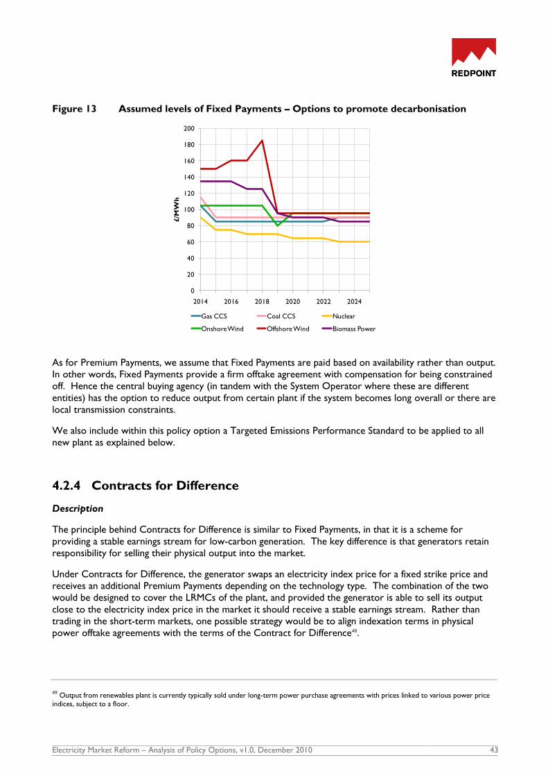
Electricity Market Reform – Analysis of Policy Options, v1.0, December 2010 43
Figure 13 Assumed levels of Fixed Payments – Options to promote decarbonisation
As for Premium Payments, we assume that Fixed Payments are paid based on availability rather than output.
In other words, Fixed Payments provide a firm offtake agreement with compensation for being constrained
off. Hence the central buying agency (in tandem with the System Operator where these are different
entities) has the option to reduce output from certain plant if the system becomes long overall or there are
local transmission constraints.
We also include within this policy option a Targeted Emissions Performance Standard to be applied to all
new plant as explained below.
4.2.4 Contracts for Difference
Description
The principle behind Contracts for Difference is similar to Fixed Payments, in that it is a scheme for
providing a stable earnings stream for low-carbon generation. The key difference is that generators retain
responsibility for selling their physical output into the market.
Under Contracts for Difference, the generator swaps an electricity index price for a fixed strike price and
receives an additional Premium Payments depending on the technology type. The combination of the two
would be designed to cover the LRMCs of the plant, and provided the generator is able to sell its output
close to the electricity index price in the market it should receive a stable earnings stream. Rather than
trading in the short-term markets, one possible strategy would be to align indexation terms in physical
power offtake agreements with the terms of the Contract for Difference49.
49
Output from renewables plant is currently typically sold under long-term power purchase agreements with prices linked to various power price
indices, subject to a floor.
2014 2016 2018 2020 2022 2024
0
20
40
60
80
100
120
140
160
180
200
£/M
Wh
Gas CCS Coal CCS Nuclear
Onshore Wind Offshore Wind Biomass Power

Electricity Market Reform – Analysis of Policy Options, v1.0, December 2010 44
As with Fixed Payments, the design of the Contracts for Difference would be different for technologies
with low and stable short-run costs (such as most renewables and nuclear), compared to technologies with
fuel input costs such as CCS and biomass.
For the former, the Contracts for Difference would be „two-way‟. If the electricity index price were to be
above the strike price, the generator would pay the difference to a central agency, and if it were below it
would receive the difference. For many types of low-carbon generation, for example wind, output levels
vary considerably and hence the CfD would need to be structured to recognise this volume variability.
How this is done has implications for the level of risk retained by the generator. If the CfD was settled at a
half-hourly level based on a within-day price index against the actual output from the generator, its risk
would be low provided it could trade its output close to the within-day index. It would, however, retain
some short-term balancing risk. The downside with this approach (also a risk with Fixed Payments) is that
it provides little differential incentive for the generator to ensure that its plant is available when prices are
higher, to forecast accurately (other than to minimise short-term balancing risk), or to site plant away from
locations where there is already a high concentration of similar plant50. In order to maintain these
incentives, an alternative approach would be to settle the CfD based (for example) on a monthly averaged
price and monthly averaged output.
The indexation terms and strike for the two-way CfD would most likely be set directly by Government.
The additional premia by technology could either be set:
via administered premium tariffs set by Government according to technology, or
by holding a competitive tender where investors in different technology classes bid for the
premia they require above the CfD strike price.
Conceptually this is the same as setting Fixed Payments, since the sum of the CfD strike and premia would
also yield an essentially fixed revenue stream. However, it does require Government implicitly to take a
long-term view of the electricity price when setting the CfD strike which may present some challenges.
The Contracts for Difference concept is more complex for plant that have significant fuel input costs such
as CCS and biomass. Because the input costs vary (based on fuel and carbon prices), a two-way CfD
against the electricity price does not stabilise earnings in the same way as for nuclear and most renewables.
Also it is possible that electricity prices may fall below short-run costs on occasions and the plant would
choose not to run.
In this case the CfD concept becomes more like a tolling agreement – the central agency pays the
generator a tolling fee for use of the plant. Effectively the generator is swapping the infra-marginal spread
(the difference between the electricity price and its SRMC) for a fixed tolling fee. In terms of financial
instruments this is equivalent to the generator selling a one-way CfD on the spread between the electricity
price and its short-run costs (defined by some form of indexation formula) and receiving a premium in
return. If the spread is positive (and the plant runs) the generator pays out the difference between the
electricity price and the fuel indexation formula. Hence, to minimise its risk the generator is incentivised to
sell its power and buy its fuel / carbon close to the respective indices. The premium that it receives would
be designed to cover the fixed and capital costs of the plant, and is equivalent to the concept of the
availability fee under Fixed Payments.
As under the two-way CfD, these premia would differ by technology and could be set by Government or
established via a competitive tender.
50
Due to the correlated nature of wind output there is likely to be an increasing relationship between windy periods and low prices. There is a
benefit to the system of having a more geographically dispersed generation mix to smooth the variability in wind output. There should also be a benefit to the generator since it should be able to „capture‟ a better price for its output under the current market arrangements.

Electricity Market Reform – Analysis of Policy Options, v1.0, December 2010 45
The net difference payments on the CfDs and the costs of the premia would be collected by the central
agency and levied (or rebated) to consumers via suppliers.
Impact on investment risk
Table 8 summarises the possible impact of Contracts for Difference on the major sources of investment
risk for low-carbon generation. Electricity revenue risk is significantly reduced, but not completely
eliminated unlike under Fixed Payments, since generators are still exposed to „basis‟ risk, the difference
between the index price against which the contract is settled and the price at which they sell their
electricity. Support level risk is very low since the Contracts for Difference approach is based around long-
term contracts.
Fuel price risk is significantly reduced for CCS and biomass generators since their CfDs are settled on the
spread between an electricity price and fuel price index. Load factor risk for nuclear, and particularly CCS
plant, would also be reduced if these plant receive their premia based on availability.
Table 8 Impact of Contracts for Difference on investment risk
Modelling assumptions
Based on the results of simulating the earnings risk for different types of investment, we make some
assumptions on the possible increase in gearing that may be achievable for different technologies under
Fixed Payments.
These assumptions are shown in Table 9 below.
CCGT Nuclear CCS Wind Biomass
Fuel costs Risk unchanged Risk unchanged Risk reduced n/a Risk reduced
Carbon costs Risk unchanged n/a n/a n/a n/a
Electricity
revenues
Risk unchanged (but
note reduction in
expected price)
Risk reduced Risk reduced Risk reduced Risk reduced
Support levels n/aNew support (no
risk)
New support (no
risk)Risk removed Risk removed
Load factor
riskRisk unchanged Risk reduced Risk reduced Risk unchanged Risk unchanged
Balancing risk Risk unchanged Risk unchanged Risk unchanged Risk unchanged Risk unchanged
Construction
costs/timesRisk unchanged Risk unchanged Risk unchanged Risk unchanged Risk unchanged
Availability/
technology riskRisk unchanged Risk unchanged Risk unchanged Risk unchanged Risk unchanged
O&M costs Risk unchanged Risk unchanged Risk unchanged Risk unchanged Risk unchanged

Electricity Market Reform – Analysis of Policy Options, v1.0, December 2010 46
Table 9 Assumptions on the possible increase in gearing under Contracts for Difference
In general, we assume that the increase in gearing possible is somewhat less than under Fixed Payments
since generators are still exposed to certain risks from selling their output. Intermittent renewables such
as wind also retain balancing risk which is not the case under Fixed Payments.
We have made a similar set of assumptions for Contracts for Difference as for Fixed Payments, namely:
contract strike prices and technology premia are set by Government and contracts cover the
economic lifetime of the plant,
a diverse range of technologies is incentivised by providing technology-differentiated premia
that bridge the different funding gaps,
the policy is implemented in 2014 with two years‟ notice, and
the combined contract strike prices and technology premia are set based on the LRMCs of the
different technologies rounded to the nearest £5/MWh.
We have also assumed the same arrangements for grandfathering the RO, and that the support for CCS
demonstration plant would be incorporated within the Contracts for Difference regime.
Figure 14 shows the level of Contracts for Difference assumed for different technologies. We have not
separated explicitly the CfD strike price from the technology premia in this illustration since for the
purposes of investment modelling it is the combined level that is important. The combined payments
follow similar paths as under Fixed Payments.
Assumed
increased in
gearing
CCGT 0%
CCGT +
CCS10%
Coal +
CCS20%
Nuclear 25%
Onshore
wind15%
Offshore
wind15%
Biomass 20%
OCGT 0%

Electricity Market Reform – Analysis of Policy Options, v1.0, December 2010 47
Figure 14 Assumed levels of Contracts for Difference including technology premia –
Options to promote decarbonisation
For the one-way CfDs for generators with non-zero SRMCs such as CCS and biomass, we have modelled
them such that generators only receive the low-carbon premia when the spread between fuel costs and
electricity prices is positive, although it could equally well be paid on availability. The way we have
modelled it leaves load factor risk with the generator requiring slightly higher premia to attract investment,
but the payments are made less often. From the modelling perspective there would be little difference
between the options, although this is an important design consideration.
We also include within this policy option a Targeted Emissions Performance Standard to be applied to all
new plant as explained below.
4.2.5 Strong Emissions Performance Standard
Description
An Emissions Performance Standard (EPS) would place limits on the amounts of carbon dioxide that could
be emitted from generating plant. Its objective would be to discourage investment in high carbon
generating plant, and thus incentivise investment in low-carbon technologies.
There are a number of different ways that an EPS could be implemented:
on a rate basis (a limit of emissions per MWh generated), or as an annual „bubble‟ (a limit on
emissions within a year),
on new plant only, or on all plant,
on specific plant types, eg coal, or on all plant types, and
at the individual plant level or on a generator‟s portfolio.
2014 2016 2018 2020 2022 2024
0
20
40
60
80
100
120
140
160
180
200
£/M
Wh
Gas CCS Coal CCS Nuclear
Onshore Wind Offshore Wind Biomass Power

Electricity Market Reform – Analysis of Policy Options, v1.0, December 2010 48
These design choices have important implications for the types of investment that are possible, the timing
of CCS retrofit decisions, how plant on the system operate, and the speed with which existing plant on the
system retire. For example, a rate-based limit on new plant may prevent investment in unabated coal plant
but allow investment in CCGTs. A rate-based limit applied to existing plant may force closures of coal
plant, whereas, under an annual „bubble‟ limit these plant may be able to stay open longer but operate at
progressively lower load factors.
Impact on investment risk
The introduction of an EPS does not directly impact the investment risk for low-carbon technologies since
these plant are still exposed to uncertain future electricity prices. However, by restricting output from
highly emitting generators this is likely to push up the expectation of future electricity prices, hence
improving expected returns for low-carbon plant.
Conversely, for highly emitting plant, the EPS may make investment untenable. For CCGTs51, the impact on
investment risk is complex. On the one hand, these plant may benefit where coal plant are squeezed out of
the merit order, while on the other hand, they themselves may become affected by a progressively
tightening limit.
Modelling assumptions
Under all policy options we assume that there is a Targeted Emissions Performance standard on new plant
as a minimum. This would be an annual limit equivalent to 600 g/kWh operating at baseload. At this level
it would prevent new unabated coal investment, and require demonstration plant to have at least 25% of
their capacity fitted with CCS. CCS units would have to run in order for the plant to be able to operate at
baseload.
Set at this level, the EPS would not be sufficient alone to drive the low-carbon investment required to
achieve a carbon intensity of 100 g/kWh by 2030. The Strong EPS policy option would therefore need to
consider capturing all plant (new and existing) and be set at a much tighter level. Our assumptions were
derived through iteration in the model.
We assume that the annual EPS limit for all plant is first introduced in 2018 at 2.39 t/kW. This is equivalent
to 275 g/kWh operating at baseload, ie significantly tighter than the Targeted EPS included in the other
policy options. At this level it would restrict the annual load factors of CCGTs to around 75% and existing
coal plant to around 30%52.
The limit is progressively tightened after 2025 such that by 2030 only fossil plant fully fitted with CCS could
operate at baseload. This is illustrated in Figure 15 below.
51
The typical emissions from a new CCGT are approximately 350 g/kWh.
52 Note that it may be necessary to exempt the unabated portions of the CCS demo projects from the EPS in order to attract the participation
required.

Electricity Market Reform – Analysis of Policy Options, v1.0, December 2010 49
Figure 15 Modelling annual EPS relative to emissions intensity of different plant types –
Options to promote decarbonisation
As the modelling results below show, the impact of this Strong EPS is to drive up electricity prices,
improving the economics of low-carbon investment, while deterring investment in fossil fuel plant. Due to
the higher electricity prices, we assume that bands under the RO can be reduced while still achieving the
targets of 29% and 35% of generation from renewable sources in 2020 and 2030. We assume that the CCS
demonstration projects would still be funded separately, but that the tighter EPS would be sufficient to
incentivise these plant fully to retrofit with CCS after 2025.
For the purposes of the modelling, we assume that there is no change in gearing / hurdle rates for low-
carbon investment associated with the Strong EPS policy.
4.3 Summary of policy impact on hurdle rates
We described above our assumptions for the increase in gearing that might be possible under each of the
decarbonisation options. Table 10 summarises the resultant hurdle rates (post-tax nominal) for typical
investors in different technologies relative to the Baseline. Further details of how hurdle rates are
calculated in the analysis are provided in Appendix D.
The table shows assumed typical rates for a utility, independent developer and a developer of nuclear plant.
The hurdle rates illustrated are based on the maturity of each technology in 2010. These maturities are
assumed to evolve over time, with corresponding changes in hurdle rates, as shown in Appendix D.
0
1
2
3
4
5
6
7
8t/
kW
Annual EPS New CCGT Existing coal plant Coal+CCS

Electricity Market Reform – Analysis of Policy Options, v1.0, December 2010 50
Table 10 Summary of hurdle rate assumptions under different decarbonisation options
Tech
maturity
(2010) Baseline CPS50 EPS PP FP CfD
Carbon Price Support (£50/t) No Yes No No No No
Emissions Performance
Standard No Targeted Strong Targeted Targeted Targeted
Capacity payments No No No No No No
Low-carbon support RO RO RO Prem Fixed CfD
Hurdle rates (typical utility)
CCGT Mature 8.1% 8.1% 8.1% 8.1% 8.1% 8.1%
CCGT+CCS Emerging 12.1% 11.7% 12.1% 11.6% 11.5% 11.6%
Coal+CCS Emerging 12.1% 11.8% 12.1% 11.5% 11.4% 11.4%
Onshore wind Mature 8.1% 8.1% 8.1% 8.1% 7.8% 7.8%
Offshore wind (R1/R2) Established 10.1% 10.1% 10.1% 10.1% 9.6% 9.6%
Offshore (R3) Emerging 12.1% 12.1% 12.1% 12.1% 11.4% 11.5%
Biomass Emerging 12.1% 11.9% 12.1% 12.1% 11.4% 11.4%
OCGT Mature 8.1% 8.1% 8.1% 8.1% 8.1% 8.1%
Hurdle rates (independent developer)
CCGT Mature 9.1% 9.1% 9.1% 9.1% 9.1% 9.1%
CCGT+CCS Emerging 13.3% 12.5% 13.3% 12.5% 12.5% 12.5%
Coal+CCS Emerging 13.3% 12.5% 13.3% 12.5% 12.5% 12.5%
Onshore wind Mature 9.1% 9.1% 9.1% 9.1% 7.8% 8.1%
Offshore wind (R1/R2) Established 11.2% 11.2% 11.2% 11.2% 10.0% 10.0%
Offshore (R3) Emerging 13.3% 13.3% 13.3% 13.3% 12.5% 12.5%
Biomass Emerging 13.3% 12.9% 13.3% 13.3% 12.5% 12.5%
OCGT Mature 9.1% 9.1% 9.1% 9.1% 9.1% 9.1%
Hurdle rates (nuclear developer)
Nuclear Emerging 13.2% 12.7% 13.2% 12.2% 11.2% 11.2%
The greatest reductions in hurdle rates occur under Fixed Payments since this policy option has the
greatest impact in reducing risk for low-carbon generators, with a reduction of up to 1.3% for onshore
wind and up to 2% for nuclear. Independent developers are generally assumed to benefit more than
vertically integrated utilities from policy options that reduce earnings risk since they are less able to
diversify their risk against a wider portfolio.
4.4 Results of modelling
In this section, we present some of the key results from the modelling of the five decarbonisation options –
Carbon Price Support (£50/t), Premium Payments, Fixed Payments, Contracts for Difference and Strong
Emissions Performance Standard – in relation to the following:
carbon dioxide emissions
plant mix
electricity prices
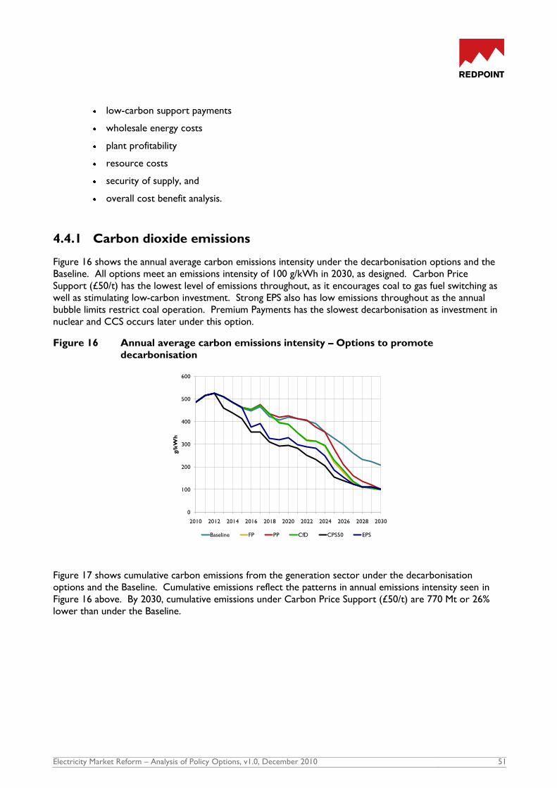
Electricity Market Reform – Analysis of Policy Options, v1.0, December 2010 51
low-carbon support payments
wholesale energy costs
plant profitability
resource costs
security of supply, and
overall cost benefit analysis.
4.4.1 Carbon dioxide emissions
Figure 16 shows the annual average carbon emissions intensity under the decarbonisation options and the
Baseline. All options meet an emissions intensity of 100 g/kWh in 2030, as designed. Carbon Price
Support (£50/t) has the lowest level of emissions throughout, as it encourages coal to gas fuel switching as
well as stimulating low-carbon investment. Strong EPS also has low emissions throughout as the annual
bubble limits restrict coal operation. Premium Payments has the slowest decarbonisation as investment in
nuclear and CCS occurs later under this option.
Figure 16 Annual average carbon emissions intensity – Options to promote
decarbonisation
Figure 17 shows cumulative carbon emissions from the generation sector under the decarbonisation
options and the Baseline. Cumulative emissions reflect the patterns in annual emissions intensity seen in
Figure 16 above. By 2030, cumulative emissions under Carbon Price Support (£50/t) are 770 Mt or 26%
lower than under the Baseline.
2010 2012 2014 2016 2018 2020 2022 2024 2026 2028 2030
0
100
200
300
400
500
600
g/k
Wh
Baseline FP PP CfD CPS50 EPS

Electricity Market Reform – Analysis of Policy Options, v1.0, December 2010 52
Figure 17 Cumulative carbon emissions from 2010 – Options to promote decarbonisation
4.4.2 Plant mix
Although the level of renewables generation is similar to that under the Baseline, each of the policy options
has more new nuclear and CCS, although the proportions of these technologies differ between the options.
The options also vary in the amount of new CCGT that is built as a consequence of the speed with which
low-carbon investment occurs.
Renewables
By adjusting renewables support levels, all decarbonisation options have been designed to achieve
approximately 29% and 35% generation from renewables by 2020 and 2030 respectively under Central
assumptions.
Figure 18 shows similar trajectories for renewables output under each of the decarbonisation options and
the Baseline. The proportions of different renewable technologies are broadly similar across the options,
although there are some variations depending on the exact level at which support has been set.
In the period 2010 to 2013, renewables are built under the RO under all options, which is then
grandfathered under the options where the RO is replaced (Premium Payments, Fixed Payments and
Contracts for Difference). We have not assumed any investment hiatus as the result of the change in
policy but this is a material risk. From 2014 onwards, renewables are built under the new policy option
although under Carbon Price Support (£50/t) and Strong EPS the RO is retained.
2010 2012 2014 2016 2018 2020 2022 2024 2026 2028 2030
0
500
1000
1500
2000
2500
3000
3500
ton
ne
s m
illi
on
Baseline FP PP CfD CPS50 EPS

Electricity Market Reform – Analysis of Policy Options, v1.0, December 2010 53
Figure 18 Proportion of generation from large scale renewables – Options to promote
decarbonisation
Nuclear and CCS
The timing and amount of investment in nuclear and CCS plant differs depending on the policy option.
Under the assumptions modelled, the first new nuclear plant becomes operational earliest under Fixed
Payments and Contracts for Difference (201953) on the back of securing long-term fixed price contracts.
Under Carbon Price Support (£50/t), Premium Payments and Strong EPS, as modelled, the first new nuclear
becomes operational in the period 2022-2024. (This result is very dependent on the assumptions made
around price levels.) By contrast the first new nuclear under the Baseline becomes operational in 2027.
The modelling suggests that nuclear is favoured over CCS when the investment incentive is purely based on
a market-wide price signal, as is the case under Carbon Price Support (£50/t). This is because it is assumed
to be lower cost and to mature earlier. Under Premium Payments, Fixed Payments and Contracts for
Difference there is a greater proportion of CCS since we assume that it would receive targeted support at
a level that bridges the different funding gaps. As a result these options tend to promote a more
diversified, but (initially) more expensive generation mix. Note that under all the policy options we assume
that CCS becomes technically proven and that it is economic to retrofit the unabated units of the
demonstration plant by 2025.
53
According to EDF, the first new reactor, which is likely to be Hinkley Point C, could become operational a year earlier than this in 2018.
2010 2012 2014 2016 2018 2020 2022 2024 2026 2028 2030
0%
5%
10%
15%
20%
25%
30%
35%
40%
Baseline FP PP CfD CPS50 EPS

Electricity Market Reform – Analysis of Policy Options, v1.0, December 2010 54
Table 11 Timing and capacity of Nuclear and CCS investment
Baseline CPS50 EPS PP FP CfD
Year of first new nuclear 2027 2022 2024 2023 2019 2019
Year of CCS demo plant
retrofit After 2030 2025 2025 2025 2025 2025
New nuclear capacity
(2030) 6.4 GW 14.4 GW 11.2 GW 9.6 GW 9.6 GW 11.2 GW
New CCS capacity (excl
Demos) (2030) 0.0 GW 0.0 GW 3.5 GW 7.0 GW 7.0 GW 5.5 GW
CCGT
The amount of investment in new CCGTs varies across the options (Figure 19). Earlier investment in
nuclear under Fixed Payments and Contracts for Difference, coupled with the assumption that the 2020
renewables target can be met, results in no further CCGT investment after 2012. Under Carbon Price
Support (£50/t), Premium Payments and Strong EPS, where nuclear investment comes later, there is
additional CCGT investment in the period 2019 to 2026 although this plant is built with lower expectations
of future load factors.
Figure 19 Cumulative new CCGT build54 – Options to promote decarbonisation
54
Note that where sections of some lines are not visible, they are hidden behind the Baseline except in the case of Fixed Payments, where new
CCGT build is identical to that under CfDs.
2010 2012 2014 2016 2018 2020 2022 2024 2026 2028 2030
0
2
4
6
8
10
12
14
16
18
20
GW
FP PP CfD CPS50 EPS Baseline

Electricity Market Reform – Analysis of Policy Options, v1.0, December 2010 55
Coal plant retirements
Under Fixed Payments, Premium Payments and Contracts for Difference, the pattern of plant retirements
is similar to the Baseline, driven by economics and restrictions under the IED. Under Carbon Price
Support (£50/t), the higher carbon price faced by generators makes coal plant less profitable and brings
about earlier closures. The Strong EPS also accelerates coal plant closures. Retirements of gas plant under
the different decarbonisation options are generally similar to the Baseline.
Figure 20 Coal plant retirements – Options to promote decarbonisation
Capacity and generation mix
Figure 21 and Figure 22 show the total capacity and generation mix respectively from the modelling for the
decarbonisation options compared to the Baseline.
Figure 21 Capacity mix – Options to promote decarbonisation
2010 2012 2014 2016 2018 2020 2022 2024 2026 2028 2030
0
5
10
15
20
25
30
GW
Baseline FP PP CfD CPS50 EPS
0
20
40
60
80
100
120
GW
GT
non ROC waste
Barrages and Tidal Range
Other renewables
Biomass
Marine
Wind
Pumped storage
Hydro
Nuclear (new)
Nuclear (existing)
CCS
Coal
Gas
2030 2020

Electricity Market Reform – Analysis of Policy Options, v1.0, December 2010 56
Figure 22 Generation mix – Options to promote decarbonisation
4.4.3 Electricity prices
Figure 23 shows the annual average baseload electricity prices from the modelling under the five
decarbonisation options compared to the Baseline. The impact is different depending on whether the
policy option provides targeted support to low-carbon generation or is designed to influence the electricity
price signal.
Increased fossil generation costs put upward pressure on electricity prices under Carbon Price Support
(£50/t) but over time the effect „wears off‟ as the average carbon intensity of the system diminishes with
increasing low-carbon generation. This change in the pass-through of the carbon costs into the electricity
price has implications for the effectiveness of Carbon Price Support as a continued signal for low-carbon
investment in the longer term.
The Strong EPS also leads to significantly higher prices in the period 2015 to 2025 since the restriction on
coal plant operation requires more generation from higher cost sources (gas plant), and because plant with
restricted operation are expected to reflect the opportunity cost of output under the annual bubble limit in
the prices they offer in the market.
In all cases the greater proportion of low-carbon generation on the system, with low SRMCs, reduces
prices relative to the Baseline in the latter part of the 2020s, although tighter capacity margins in some
years counter this effect. This is discussed further in Section 4.4.8 below.
As explained above, we have assumed that plant receive Fixed Payments or Premium Payments based on
availability rather than output. There is an increasing risk that under an output-based mechanism prices
could become negative at times when output from low-carbon generation exceeds demand as low-carbon
generators compete to keep running to receive their support payments. This would lead to significantly
lower electricity prices with possible negative implications for security of supply.
0
50
100
150
200
250
300
350
400
TW
h
Interconnector
GT
non ROC waste
Barrages and Tidal Range
Other renewables
Biomass
Marine
Wind
Pumped storage
Hydro
Nuclear (new)
Nuclear (existing)
CCS
Coal
Gas
2030 2020

Electricity Market Reform – Analysis of Policy Options, v1.0, December 2010 57
Figure 23 Annual average baseload electricity prices – Options to promote
decarbonisation
4.4.4 Low-carbon support payments
The amount of low-carbon support payments differs between the different policy options. Low-carbon
support payments include the total of RO costs (including any grandfathering costs), Levy Exemption
Certificates (LECs) and any payments from Premium Payments, Fixed Payments or Contracts for
Difference.
Figure 24 compares the total annual low-carbon support payments across the decarbonisation policy
options compared to the Baseline. Payments are highest under Fixed Payments and Contracts for
Difference55, and lowest under Carbon Price Support (£50/t) and Strong EPS where low-carbon support is
limited to the RO and Levy Exemption Certificates56.
55
For CfDs we show the total payments as the combination of the CfD strike price and technology premia.
56 We have assumed that the Climate Change Levy is retained, although it may be replaced as part of the introduction of Carbon Price Support or
other policy options.
2010 2012 2014 2016 2018 2020 2022 2024 2026 2028 2030
0
20
40
60
80
100
120
£/M
Wh
Baseline FP PP CfD CPS50 EPS

Electricity Market Reform – Analysis of Policy Options, v1.0, December 2010 58
Figure 24 Gross annual low-carbon payments to generators – Options to promote
decarbonisation
To make comparison between the options easier, Figure 25 shows the „net‟ low-carbon payments, which
subtract the forsaken wholesale electricity market revenues for generators operating under Fixed
Payments, and the electricity revenues for plant operating under Contracts for Difference. On a net basis,
the analysis suggests that low-carbon support is greater on average under Premium Payments than under
Fixed Payments or Contracts for Difference. This is because if electricity prices rise, as is the case in this
analysis, support for plant operating under Contracts for Difference reduces since generators pay out more
in difference payments. Similarly, the implied net support for plant operating under Fixed Payments also
reduces in this case. However, the level of support received under Premium Payments does not adjust in
response to increasing electricity prices. The opposite result would be observed if electricity prices were
to fall.
Although net payments to low-carbon generators are lower under Strong EPS and Carbon Price Support
(£50/t), consumers are exposed to higher wholesale electricity prices under these options.
Figure 25 Net annual payments to low-carbon generators – Options to promote
decarbonisation
2010 2012 2014 2016 2018 2020 2022 2024 2026 2028 2030
0
5000
10000
15000
20000
25000
£m
Baseline FP PP CfD CPS50 EPS
2010 2012 2014 2016 2018 2020 2022 2024 2026 2028 2030
0
2000
4000
6000
8000
10000
12000
£m
Baseline FP PP CfD CPS50 EPS

Electricity Market Reform – Analysis of Policy Options, v1.0, December 2010 59
4.4.5 Wholesale energy costs
Figure 26 shows the wholesale energy costs under each of the decarbonisation options compared to the
Baseline. Wholesale energy costs include the price of wholesale electricity on a demand-weighted basis,
balancing system use of system charges, and the cost of low-carbon support. Currently wholesale energy
costs represent about 40% of an average domestic consumers‟ bill, the other components being network
charges, supplier costs and margins and VAT. Under the Baseline assumptions, wholesale energy costs
would approximately double between 2010 and 2030.
Wholesale energy costs are initially higher under the decarbonisation options than the Baseline in all cases
but then fall lower after 2025. In general, consumers pay more for the low-carbon support in the early
years but then benefit from lower (and more stable) electricity prices in the long-run as the short-run
generation costs of the system decrease. Wholesale energy costs are greatest in the near term under
Carbon Price Support (£50/t) and Strong EPS due to the higher electricity prices, but in the long-run are
lower given the lower levels of low-carbon support under these policy options.
The longer-term benefits to consumers of lower wholesale electricity prices would be greater but for a
reduction in capacity margins (as discussed below) which tends to push prices up in certain years.
Figure 26 Annual average wholesale energy costs – Options to promote decarbonisation
Figure 27 shows the average wholesale energy costs over the period 2010 to 2030 under each of the
options. Prices are higher on average under Carbon Price Support (£50/t), Strong EPS and Premium
Payments, compared to the Baseline. Average wholesale energy costs for Fixed Payments and Contracts
for Difference are very similar to the Baseline. Under Fixed Payments wholesale costs are £0.13/MWh
higher and under Contracts for Difference £0.33/MWh lower than the Baseline on average.
In terms of the average domestic consumer bill, the impacts of the different options range from a £1 per
year average saving under Contracts for Difference, to a £12 per year average increase under Carbon Price
Support (£50/t)57. By way of context, the cost of low-carbon support already included in the Baseline,
57
The calculation of impact on the average domestic consumer bill is based on an annual electricity consumption level of 3.3 MWh. This
assumption is made throughout this document where the impact of a given change on the average domestic consumer bill is stated.
2010 2012 2014 2016 2018 2020 2022 2024 2026 2028 2030
0
20
40
60
80
100
120
140
160
£/M
Wh
Baseline FP PP CfD CPS50 EPS
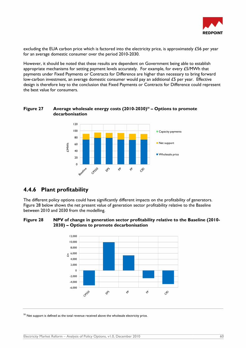
Electricity Market Reform – Analysis of Policy Options, v1.0, December 2010 60
excluding the EUA carbon price which is factored into the electricity price, is approximately £56 per year
for an average domestic consumer over the period 2010-2030.
However, it should be noted that these results are dependent on Government being able to establish
appropriate mechanisms for setting payment levels accurately. For example, for every £5/MWh that
payments under Fixed Payments or Contracts for Difference are higher than necessary to bring forward
low-carbon investment, an average domestic consumer would pay an additional £5 per year. Effective
design is therefore key to the conclusion that Fixed Payments or Contracts for Difference could represent
the best value for consumers.
Figure 27 Average wholesale energy costs (2010-2030)58 – Options to promote
decarbonisation
4.4.6 Plant profitability
The different policy options could have significantly different impacts on the profitability of generators.
Figure 28 below shows the net present value of generation sector profitability relative to the Baseline
between 2010 and 2030 from the modelling.
Figure 28 NPV of change in generation sector profitability relative to the Baseline (2010-
2030) – Options to promote decarbonisation
58
Net support is defined as the total revenue received above the wholesale electricity price.
0
20
40
60
80
100
120
£/M
Wh
Capacity payments
Net support
Wholesale price
-6,000
-4,000
-2,000
0
2,000
4,000
6,000
8,000
10,000
12,000
£m

Electricity Market Reform – Analysis of Policy Options, v1.0, December 2010 61
The higher electricity prices are the key driver of the large increase in profitability of the generation sector
under Strong EPS. By contrast, generation sector profitability is lower under Carbon Price Support (£50/t)
than the Baseline. This is due mainly to the costs to fossil generators of the carbon price floor. At the
same time some generation plant, in particular existing nuclear and renewables, could be significantly more
profitable under Carbon Price Support (£50/t).
Under Premium Payments, generation sector profitability is higher than the Baseline between 2010 and
2030. This is partly a function of the assumptions used with increasing electricity prices to 2030. Premia
are set based on lower expectations of electricity prices, and then when they subsequently rise low-carbon
generators are able to earn economic rents. (This is also a feature of the Baseline for renewables
generators.) However, these generators are also exposed to longer-term price erosion as increasing
proportions of low SRMC generation on the system could start to push prices down, although this effect
only starts to manifest itself towards the end of the modelling period in 2030.
Low-carbon generators are not able to benefit from increasing electricity prices under Fixed Payments and
Contracts for Difference and hence generation sector profitability is lower under these options than the
Baseline. However, this result does assume that Government is able to implement mechanisms that can set
payment levels close to the long-run costs of different technologies.
Economic rents for new renewables generators
One key driver of the differences in generation sector profitability under the different policy options
relative to the Baseline is the risk of economic rents for renewables generators. Under the Baseline
assumptions of rising gas and carbon prices, there is a significant risk of large rents accruing for renewables
generators whose support levels (ROC band) may have been set (and subsequently grandfathered) when
prevailing prices were lower. Figure 29 compares the annual total economic rent for new renewable
generators (ie, excluding plant already operating under the RO) in each option relative to the Baseline. To
the extent that rents can be minimised while renewables targets are still met, the cost to consumers should
be reduced.
In general over the long-run, the analysis suggests that rents for new renewables should be lower under the
decarbonisation options being considered, although in some cases they may be higher in the near term.
The additional low-carbon generation on the system under the decarbonisation options reduces prices in
the long-term relative to the Baseline (the „price erosion‟ effect). Hence, where renewables receive
premium support (CPS50, EPS and PP) rents are lower. Carbon Price Support (£50/t) allows for lower
ROC bands and hence rents are much lower than the Baseline when carbon prices subsequently rise.
Rents are also lower in the long-term under Fixed Payments and Contracts for Difference since revenues
are largely fixed for renewables whereas they are rising under the Baseline. Under Fixed Payments, rents
could be higher in the near term depending on how close prices can be set to the long-run costs of
different types of plant. This is a material risk with this policy.
Rents appear generally lower under Contracts for Difference relative to Fixed Payments since plant remain
exposed to balancing risk, and for wind plant in particular there is deteriorating price capture over time
given the increased concentration of wind on the system59. If payment levels need to be increased to
compensate for these risks, then this apparent benefit of Contracts for Difference over Fixed Payments in
terms of consumer impacts may be lower.
59
We have assumed that the CfDs settle against monthly average volumes and monthly averaged day-ahead electricity prices. As the proportion of
wind on the system increases there will be a growing negative correlation between wind output levels and price. Hence, the price that wind plant actually achieve and the price that the CfDs settle will diverge over time.

Electricity Market Reform – Analysis of Policy Options, v1.0, December 2010 62
Under Premium Payments, rents increase when wholesale prices rise due to tighter capacity margins (for
example in 2024 and 2025 in this illustration), unlike the situation for Fixed Payments and Contracts for
Difference.
Figure 29 Change in annual rents for new renewables relative to the Baseline – Options
to promote decarbonisation
4.4.7 Resource costs
Figure 30 shows the change in different elements of resource costs relative to the Baseline. These include
carbon costs, generation costs (which include fuel and operating costs) and new plant capital costs60.
Under all the decarbonisation options the total resource costs are higher than the Baseline, although the
breakdown in the change of resource costs is quite different under the different decarbonisation options.
Under Fixed Payments and Contracts for Difference, new plant capital expenditure is greatest, adding
approximately £24bn on a net present value basis to the £75bn incurred under the Baseline. This is a
consequence of accelerated investment and a relatively expensive generation mix, featuring more CCS and
less nuclear than other options. However, this increase in capital expenditure is offset by the lower hurdle
rate assumptions, which saves around £4bn over the period 2010-2030 relative to the Baseline. The result
of accelerated low-carbon investment is that the combined carbon and generation costs savings are
greatest under these options. This means that despite the higher capital expenditure, overall increases in
resource costs are lowest under these two options.
Later low-carbon investment under Premium Payments leads to lower levels of new plant capital
expenditure but also lower savings in generation and carbon costs. Carbon Price Support (£50/t) and
Strong EPS have the greatest increase in resource costs relative to the Baseline due in part to the higher
generation costs caused by greater use of gas which is more expensive than coal generation under the
Central assumptions.
60
Capital costs are annuitised based on hurdle rates of investment, and then discounted over the period 2010-2030 using a Government Green
Book discount rate of 3.5% real. All assumptions and results are in 2009 real terms.
2010 2012 2014 2016 2018 2020 2022 2024 2026 2028 2030
-3500
-3000
-2500
-2000
-1500
-1000
-500
0
500
1000
1500
2000
£m
FP PP CfD CPS50 EPS

Electricity Market Reform – Analysis of Policy Options, v1.0, December 2010 63
Changes in resource costs relative to the total wholesale energy cost of electricity are small in percentage
terms, ranging from a 0.8% increase under Fixed Payments and Contracts for Difference to a 1.7% increase
under Strong EPS. The results are sensitive to the exact generation mix and the timing of investment which
can be affected by the design of each policy option.
Figure 30 Change in resource costs relative to the Baseline – Options to promote
decarbonisation
-30000
-20000
-10000
0
10000
20000
30000
£m
Carbon costs Generation costs
Capital costs Total change in resource costs

Electricity Market Reform – Analysis of Policy Options, v1.0, December 2010 64
4.4.8 Security of supply
Figure 31 shows the annual de-rated capacity margins produced by the modelling under the decarbonisation
options relative to the Baseline.
Figure 31 Annual de-rated capacity margin – Options to promote decarbonisation
Analysis of the Baseline suggested that there may be material risks to security of supply by the end of the
decade. The effect of increasing proportions of low-carbon generation on the system is likely further to
depress electricity prices, and deter investment in conventional generation. The risk appears to be greatest
under the targeted low-carbon support options (Premium Payments, Fixed Payments, Contracts for
Difference) in the period to 2025, before the bulk of the new low-carbon investment comes on line.
Under Carbon Price Support (£50/t), there is more investment in new CCGTs which are able to earn a
reasonable return with the higher wholesale prices, although some coal plant closes earlier. Under Strong
EPS, coal plant do not necessarily close earlier since they are able to benefit from the higher peak prices
associated with the tighter capacity margins. It is profitable for them to remain open operating under the
TNP until 2020 and then under a derogation under the IED. However, if the Strong EPS, affecting all plant,
was implemented as a rate limit rather than a bubble limit it is more likely that coal plant would close
earlier.
Figure 32 shows the levels of expected energy unserved for the decarbonisation options. The risk of
unserved energy is significantly greater than under the Baseline and appears highest under Fixed Payments,
Premium Payments and Contracts for Difference, in the mid-2020s. Carbon Price Support (£50/t) and
Strong EPS have a similar level of expected energy unserved to the Baseline.
2010 2012 2014 2016 2018 2020 2022 2024 2026 2028 2030
0%
5%
10%
15%
20%
25%
30%
Baseline FP PP CfD CPS50 EPS

Electricity Market Reform – Analysis of Policy Options, v1.0, December 2010 65
Figure 32 Expected Energy Unserved – Options to promote decarbonisation
4.4.9 Cost benefit analysis of decarbonisation options
Table 12 summarises the cost benefit analysis for the period 2010 to 2030, in net present value terms61.
Further explanations of the cost benefit calculation are provided in Appendix G. All five decarbonisation
options show a small reduction in net welfare to 2030, largely because the costs of new low-carbon
investment are somewhat higher than the cost of carbon saved to this point. The decrease in net welfare
as a proportion of the total wholesale costs of electricity over the period is between 0.8 and 1.7%. As
shown in Figure 33 below, by 2030, Carbon Price Support (£50/t), Fixed Payments and Contracts for
Difference are showing a net welfare gain on an annual basis.
61
Note that the cost benefit analysis does not include any assessment of the impact on air quality of the different packages.
2010 2012 2014 2016 2018 2020 2022 2024 2026 2028 2030
0
5
10
15
20
25
30
35G
Wh
Baseline FP PP CfD CPS50 EPS

Electricity Market Reform – Analysis of Policy Options, v1.0, December 2010 66
Table 12 Decarbonisation options relative to Baseline, NPV 2010-203062
Differences in net welfare are predominantly driven by changes in resource costs (carbon, generation and
capital costs) and hence Fixed Payments and Contracts for Difference appear the most favourable on this
basis. There are small variations between the options with respect to welfare gains and losses associated
with short-term demand elasticity63, both involuntary (unserved energy) and voluntary (demand side
response). Welfare losses here suggest a lower level of security of supply relative to the Baseline.
Larger changes are apparent in welfare distribution. Consumer surplus is lower under Carbon Price
Support (£50/t), Strong EPS, and Premium Payments relative to the Baseline. Under Carbon Price Support
(£50/t) and Strong EPS the reduction in consumer surplus results from the higher wholesale electricity
prices (offset to a degree by lower low-carbon payments). Under Premium Payments, the loss of
consumer surplus is largely the result of higher low-carbon payments. The additional costs under Fixed
Payments are low, and under Contracts for Difference there may be a small benefit to consumers.
Producer surplus declines under Carbon Price Support (£50/t), Fixed Payments and Contracts for
Difference, but increases under Strong EPS and Premium Payments for the reasons outlined above in the
discussion of generation sector profitability above. With Carbon Price Support (£50/t) there would be
additional Treasury receipts (not shown) associated with the carbon price floor.
Figure 33 shows the net welfare in each year, from 2010 to 2030 (in 2009 real terms). This shows a similar
pattern under all the decarbonisation options, namely that the costs of accelerating low-carbon investment
outweigh the benefits in terms of net welfare in the near term. However, once the carbon price starts to
rise sharply, the trend reverses and by the end of the 2020s there is a net welfare benefit under most
options. With an increasing carbon price after 2030, we may expect all policies to deliver enduring net
welfare benefits.
62
Excluded from this table are changes in tax revenues associated the Climate Change Levy and Carbon Price Support.
63 For simplicity we have not included long-term demand elasticity within the analysis.
Change in welfare
NPV 2010-2030,
(£m 2009 real)
Carbon Price
Support (£50/t)
Strong
Emissions
Performance
Standard
Premium
PaymentsFixed Payments
Contracts for
Difference
Carbon costs 15,758 13,081 6,037 9,806 9,637
Generation costs -4,098 -4,400 3,828 10,492 10,790
Capital costs -17,496 -16,496 -16,337 -23,920 -24,105
Unserved energy 44 93 -212 -207 -265
Demand side response 12 16 -15 -18 -23
Change in Net Welfare -5,780 -7,706 -6,698 -3,846 -3,965
Wholesale price -30,545 -27,420 -1,257 3,316 611
Low carbon payments 7,474 9,811 -10,533 -4,237 437
Capacity payments 0 0 0 0 0
Unserved energy 44 93 -212 -207 -265
Demand side response 12 16 -15 -18 -23
Change in Consumer Surplus -23,015 -17,499 -12,017 -1,146 760
Wholesale price 30,545 27,420 1,257 -3,316 -611
Low carbon support -7,535 -9,691 10,532 4,266 -434
Capacity payments 0 0 0 0 0
Producer costs -28,190 -7,815 -6,471 -3,621 -3,678
Change in Producer Surplus -5,180 9,914 5,318 -2,671 -4,722
Net Welfare
Distributional analysis
Consumer
Surplus
Producer Surplus

Electricity Market Reform – Analysis of Policy Options, v1.0, December 2010 67
Figure 33 Annual Net welfare change relative to Baseline – Options to promote
decarbonisation
4.5 Sensitivity analysis
4.5.1 Overview
In order to test the outcomes of the analysis to key uncertainties, we have modelled a number of
sensitivities on commodity prices, and investor confidence in Carbon Price Support.
4.5.2 Commodity price sensitivities
All five decarbonisation options have been designed to achieve 29% and 35% generation from renewables in
2020 and 2030 respectively, and a carbon intensity of 100 g/kWh by 2030, under Central assumptions.
Under different sets of assumptions the levels of decarbonisation achieved may be higher or lower under
each option. We have explored the following sensitivities on commodity prices:
High Gas - higher gas prices, reaching almost 100 p/th by 2020 and continuing at this level
until 2030,
Low Gas - lower gas prices, gradually rising to 35p/th in 2030, and
Low-carbon - lower EUA prices, below £9/tCO2 until 2020 and reaching £35/tCO2 in 2030.
These assumptions are shown in Figure 34 and Figure 35.
2010 2012 2014 2016 2018 2020 2022 2024 2026 2028 2030
-2500
-2000
-1500
-1000
-500
0
500
1000
1500£m
FP PP CfD CPS50 EPS

Electricity Market Reform – Analysis of Policy Options, v1.0, December 2010 68
Figure 34 Gas price sensitivity assumptions
Figure 35 Carbon price sensitivity assumptions
We have run each sensitivity for the Baseline and the five decarbonisation options. We show the
sensitivity under each option compared to the corresponding sensitivity in the Baseline. The key results
are the robustness of each option under the sensitivities, both in term of decarbonisation and security of
supply, and also the risk of higher costs for consumers.
We have held the price levels for Premium Payments, Fixed Payments and Contracts for Difference
constant under the sensitivities, at the same level as under the Central assumptions64, and the levels of
Carbon Price Support and assumptions on the Strong EPS are unchanged. In reality, it is likely that some
adjustments to policy would be made in response to different outturn commodity prices, and hence the
results for the sensitivities could be regarded as extreme outcomes. However, they provide useful
illustrations of the risk under each policy.
64
We assume that the utilisation payments under Fixed Payments and the strike prices under Contracts for Difference are indexed to fuel prices
and so these will adjust automatically. However, the availability payments remain constant.
0
20
40
60
80
100
120
2010
2012
2014
2016
2018
2020
2022
2024
2026
2028
2030
2032
2034
2036
2038
2040
p/t
h High
Central
Low
0
20
40
60
80
100
120
140
160
2010
2012
2014
2016
2018
2020
2022
2024
2026
2028
2030
2032
2034
2036
2038
2040
£/t
Central
Low

Electricity Market Reform – Analysis of Policy Options, v1.0, December 2010 69
4.5.3 Low Gas Sensitivity
Carbon dioxide emissions
Since gas prices are a strong driver of electricity prices, lower gas prices have a significant impact on the
trajectory of carbon dioxide emissions. In the near term there is coal to gas switching, leading to lower
emissions under all policy options, but in the longer term the lower gas prices may result in less low-carbon
investment under some policy options due to lower wholesale electricity prices.
Figure 36 shows the carbon dioxide emissions intensity under the Low Gas sensitivity for the Baseline and
each of the five decarbonisation options. Emissions intensity for the Baseline under Central assumptions is
also shown for comparison. The emissions intensity is much lower over the next decade under the Low
Gas price sensitivity as a result of the increased competitiveness of gas-fired generation, compared to the
Central assumptions which are more coal favouring. However, the pace of decarbonisation slows under
some policy options.
Only under Fixed Payments and Contracts for Difference is a carbon intensity of 100 g/kWh achieved by
2030. Under these options, low-carbon generation is not exposed to the electricity price and so
investment is broadly unaffected. Carbon Price Support (£50/t), Strong EPS and Premium Payments are
less effective in stimulating low-carbon investment when gas prices are lower, as a result of lower
electricity prices.
Figure 36 Annual average carbon dioxide emissions intensity – Options to promote
decarbonisation (Low Gas Sensitivity)
Wholesale energy costs
Figure 37 shows wholesale energy costs for the Low Gas sensitivity. Wholesale energy cost levels are
lower than under Central assumptions as a result of lower gas prices driving lower electricity prices. Fixed
Payments and Contracts for Difference are generally more expensive under the Low Gas price sensitivity
but still deliver the decarbonisation objectives, which are not achieved under the options with premium
support – Carbon Price Support (£50/t), Strong EPS and Premium Payments.
2010 2012 2014 2016 2018 2020 2022 2024 2026 2028 2030
0
100
200
300
400
500
600
g/k
Wh
Baseline FP PP CfD CPS50 EPS Baseline (Central)

Electricity Market Reform – Analysis of Policy Options, v1.0, December 2010 70
The net support element of wholesale energy costs under Fixed Payments and Contracts for Difference
implicitly adjusts to the changing underlying electricity prices, whereas under the premium support options
this is largely fixed.
Figure 37 Average wholesale energy cost – Options to promote decarbonisation (Low
Gas Sensitivity)
Security of supply
Figure 38 shows the de-rated peak capacity margins under the Low Gas sensitivity. The risks to security of
supply appear to increase materially under lower gas prices as a result of earlier closures of coal plant in
the period 2016 to 2020 due to these plant no longer being profitable.
The risk appears greatest under Fixed Payments and Contracts for Difference where investment in CCGTs
is deterred by the early deployment of nuclear and CCS. In the longer run, the de-rated capacity margins
in the model recover as investors react to the tight capacity margins and more low-carbon generation is
commissioned.
0
20
40
60
80
100
120
£/M
Wh
Wholesale price Net support
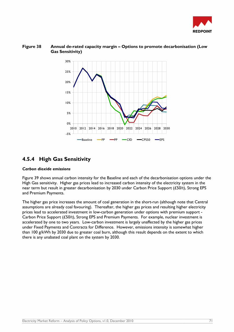
Electricity Market Reform – Analysis of Policy Options, v1.0, December 2010 71
Figure 38 Annual de-rated capacity margin – Options to promote decarbonisation (Low
Gas Sensitivity)
4.5.4 High Gas Sensitivity
Carbon dioxide emissions
Figure 39 shows annual carbon intensity for the Baseline and each of the decarbonisation options under the
High Gas sensitivity. Higher gas prices lead to increased carbon intensity of the electricity system in the
near term but result in greater decarbonisation by 2030 under Carbon Price Support (£50/t), Strong EPS
and Premium Payments.
The higher gas price increases the amount of coal generation in the short-run (although note that Central
assumptions are already coal favouring). Thereafter, the higher gas prices and resulting higher electricity
prices lead to accelerated investment in low-carbon generation under options with premium support -
Carbon Price Support (£50/t), Strong EPS and Premium Payments. For example, nuclear investment is
accelerated by one to two years. Low-carbon investment is largely unaffected by the higher gas prices
under Fixed Payments and Contracts for Difference. However, emissions intensity is somewhat higher
than 100 g/kWh by 2030 due to greater coal burn, although this result depends on the extent to which
there is any unabated coal plant on the system by 2030.
2010 2012 2014 2016 2018 2020 2022 2024 2026 2028 2030
-5%
0%
5%
10%
15%
20%
25%
30%
Baseline FP PP CfD CPS50 EPS
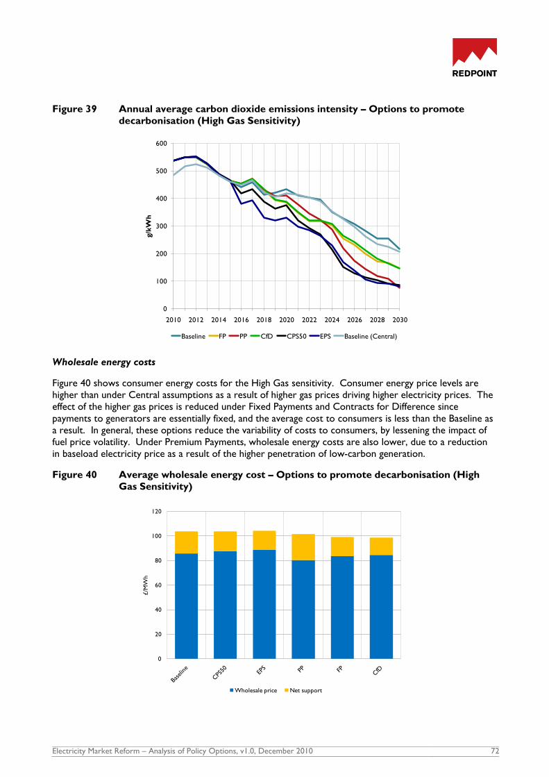
Electricity Market Reform – Analysis of Policy Options, v1.0, December 2010 72
Figure 39 Annual average carbon dioxide emissions intensity – Options to promote
decarbonisation (High Gas Sensitivity)
Wholesale energy costs
Figure 40 shows consumer energy costs for the High Gas sensitivity. Consumer energy price levels are
higher than under Central assumptions as a result of higher gas prices driving higher electricity prices. The
effect of the higher gas prices is reduced under Fixed Payments and Contracts for Difference since
payments to generators are essentially fixed, and the average cost to consumers is less than the Baseline as
a result. In general, these options reduce the variability of costs to consumers, by lessening the impact of
fuel price volatility. Under Premium Payments, wholesale energy costs are also lower, due to a reduction
in baseload electricity price as a result of the higher penetration of low-carbon generation.
Figure 40 Average wholesale energy cost – Options to promote decarbonisation (High
Gas Sensitivity)
2010 2012 2014 2016 2018 2020 2022 2024 2026 2028 2030
0
100
200
300
400
500
600g/k
Wh
Baseline FP PP CfD CPS50 EPS Baseline (Central)
0
20
40
60
80
100
120
£/M
Wh
Wholesale price Net support

Electricity Market Reform – Analysis of Policy Options, v1.0, December 2010 73
Security of supply
Figure 41 shows the de-rated peak capacity margins for each of the decarbonisation options and the
Baseline under the High Gas sensitivity. The risks to security of supply are less than under the Low Gas
price sensitivity and are similar to those under the Central assumptions.
Figure 41 Annual de-rated capacity margin – Options to promote decarbonisation (High
Gas Sensitivity)
4.5.5 Low Carbon Sensitivity
Carbon dioxide emissions
Figure 42 shows emissions intensity for the decarbonisation options and the Baseline under the Low
Carbon sensitivity. Carbon Price Support (£50/t) and Strong EPS counter the effect of a lower EUA price
but the 100 g/kWh carbon intensity is not achieved under the other policy options.
Carbon emissions are largely unaffected by the lower EUA price under Carbon Price Support (£50/t) –
although this result assumes that investors have full confidence in the CPS. We explore a sensitivity to this
below. Under Strong EPS, emissions are capped and hence the lower carbon price also has little impact on
the speed of decarbonisation.
Under Premium Payments there is less low-carbon investment as a result of the lower EUA price.
Although low-carbon investment is similar to the Central assumptions for Fixed Payments and Contracts
for Difference, there is more unabated coal and gas burn and lower load factors for CCS plant. Hence,
under these policy options the 100 g/kWh carbon intensity is also not achieved by 2030.
2010 2012 2014 2016 2018 2020 2022 2024 2026 2028 2030
0%
5%
10%
15%
20%
25%
30%
Baseline FP PP CfD CPS50 EPS

Electricity Market Reform – Analysis of Policy Options, v1.0, December 2010 74
Figure 42 Annual average carbon dioxide emissions intensity – Options to promote
decarbonisation (Low Carbon Sensitivity)
Wholesale energy costs
Figure 43 shows consumer energy prices for the Low Carbon sensitivity. Wholesale energy costs are
highest under Carbon Price Support (£50/t) – the carbon prices faced by generators, and therefore passed
through to consumers, are unchanged from the Central assumptions given the price floor. Fixed Payments
and Contracts for Difference have the lowest cost to consumers. However, under this sensitivity they do
not deliver the decarbonisation targets whereas Strong EPS and Carbon Price Support (£50/t) do.
Figure 43 Annual average wholesale energy costs – Options to promote decarbonisation
(Low Carbon Sensitivity)
2010 2012 2014 2016 2018 2020 2022 2024 2026 2028 2030
0
100
200
300
400
500
600g/k
Wh
Baseline FP PP CfD CPS50 EPS Baseline (Central)
0
20
40
60
80
100
120
£/M
Wh
Wholesale price Net support
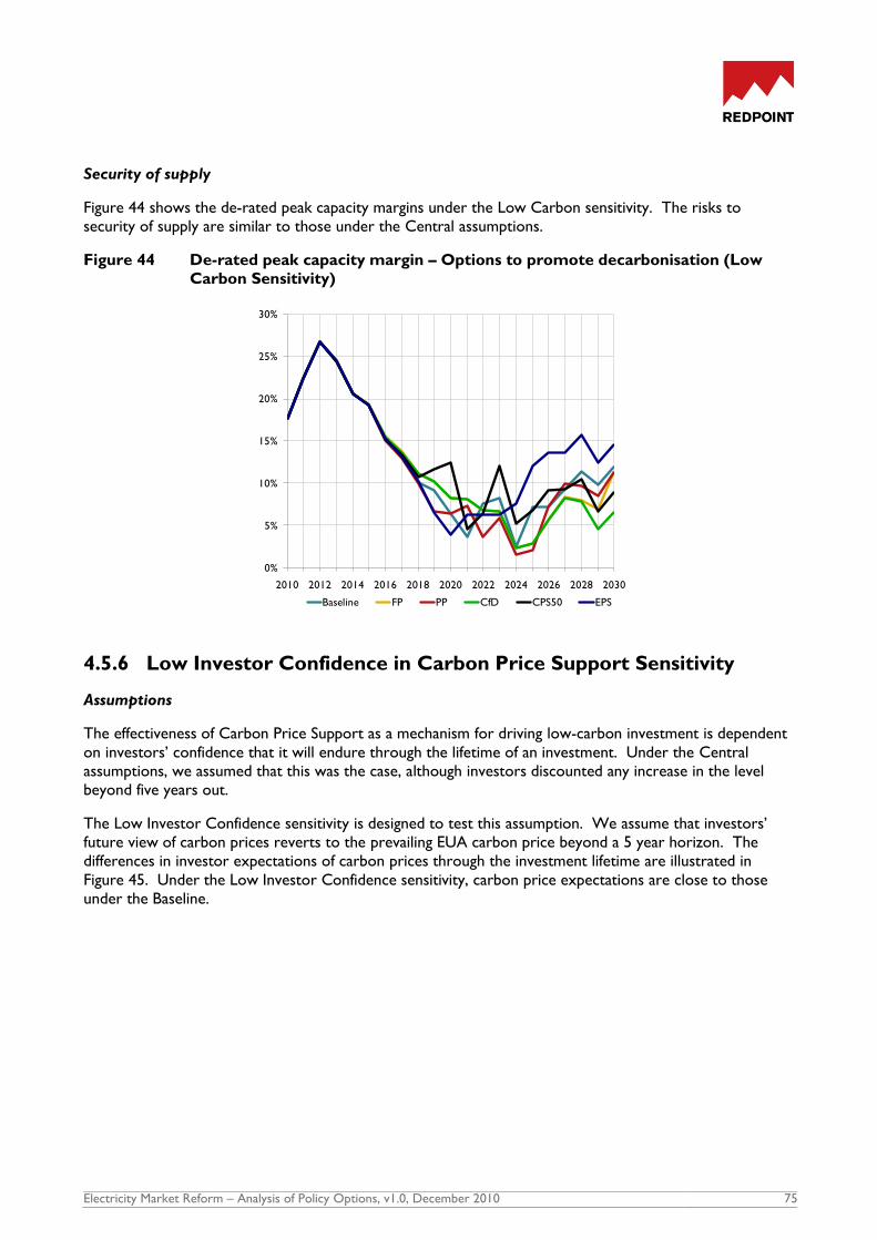
Electricity Market Reform – Analysis of Policy Options, v1.0, December 2010 75
Security of supply
Figure 44 shows the de-rated peak capacity margins under the Low Carbon sensitivity. The risks to
security of supply are similar to those under the Central assumptions.
Figure 44 De-rated peak capacity margin – Options to promote decarbonisation (Low
Carbon Sensitivity)
4.5.6 Low Investor Confidence in Carbon Price Support Sensitivity
Assumptions
The effectiveness of Carbon Price Support as a mechanism for driving low-carbon investment is dependent
on investors‟ confidence that it will endure through the lifetime of an investment. Under the Central
assumptions, we assumed that this was the case, although investors discounted any increase in the level
beyond five years out.
The Low Investor Confidence sensitivity is designed to test this assumption. We assume that investors‟
future view of carbon prices reverts to the prevailing EUA carbon price beyond a 5 year horizon. The
differences in investor expectations of carbon prices through the investment lifetime are illustrated in
Figure 45. Under the Low Investor Confidence sensitivity, carbon price expectations are close to those
under the Baseline.
2010 2012 2014 2016 2018 2020 2022 2024 2026 2028 2030
0%
5%
10%
15%
20%
25%
30%
Baseline FP PP CfD CPS50 EPS

Electricity Market Reform – Analysis of Policy Options, v1.0, December 2010 76
Figure 45 Carbon price expectations – Low Investor Confidence in Carbon Price Support
Sensitivity
We also assume that lower investor confidence means that investors perceive no reduction in investment
risk under Carbon Price Support. Therefore we assume no increase in gearing and that hurdle rates are
the same as in the Baseline.
Carbon dioxide emissions
Figure 46 shows the annual average carbon emission intensity for the Low Investor Confidence sensitivity.
Emissions intensity is the same as under Carbon Price Support (£50/t) until 2020. The main reason for this
is that the outturn Carbon Price Support level is the same and so coal to gas switching occurs to the same
extent. After 2020, carbon intensity is higher in the Low Investor Confidence sensitivity because there is
less investment in nuclear, due to lower carbon price expectations.
2010 2012 2014 2016 2018 2020 2022 2024 2026 2028 2030
0
10
20
30
40
50
60
70
80£/t
on
ne
Baseline carbon price
CPS50 Support level
CPS50 Expected carbon price
CPS50 Expected carbon price (Low Investor Confidence)

Electricity Market Reform – Analysis of Policy Options, v1.0, December 2010 77
Figure 46 Annual average carbon emissions intensity – Low Investor Confidence in
Carbon Price Support Sensitivity
Impact on plant mix
Figure 47 shows new capacity in 2020 and 2030. A key impact of low investor confidence in Carbon Price
Support is that it leads to lower investment in nuclear and renewables and greater investment in CCGTs.
Investment in nuclear is similar to the Baseline, suggesting that Carbon Price Support has little effect if
investors have no confidence in it.
Figure 47 New build 2020 and 2030 – Low Investor Confidence in Carbon Price Support
Sensitivity
Figure 48 shows new renewables capacity in 2020 and 2030. Investment in renewables is actually lower
than in the Baseline. This is because we assume that Government sets ROC bands based on full confidence
in Carbon Price Support, which are therefore lower than the ROC bands in the Baseline. Investors do not
share this confidence in Carbon Price Support, resulting in lower levels of investment.
2010 2012 2014 2016 2018 2020 2022 2024 2026 2028 2030
0
100
200
300
400
500
600
g/k
Wh
Baseline CPS50 CPS50-LowConfidence
0
10,000
20,000
30,000
40,000
50,000
60,000
70,000
MW
Renewables
Nuclear
Unabated Demo
Demo CCS
Coal - ASC with FGD & CCS
Coal - IGCC with CCS
Gas - CCGT with CCS
CCGT
2020 2030
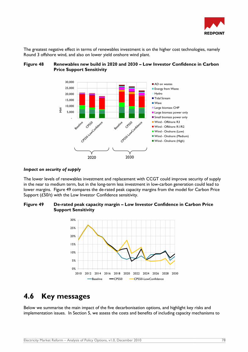
Electricity Market Reform – Analysis of Policy Options, v1.0, December 2010 78
The greatest negative effect in terms of renewables investment is on the higher cost technologies, namely
Round 3 offshore wind, and also on lower yield onshore wind plant.
Figure 48 Renewables new build in 2020 and 2030 – Low Investor Confidence in Carbon
Price Support Sensitivity
Impact on security of supply
The lower levels of renewables investment and replacement with CCGT could improve security of supply
in the near to medium term, but in the long-term less investment in low-carbon generation could lead to
lower margins. Figure 49 compares the de-rated peak capacity margins from the model for Carbon Price
Support (£50/t) with the Low Investor Confidence sensitivity.
Figure 49 De-rated peak capacity margin – Low Investor Confidence in Carbon Price
Support Sensitivity
4.6 Key messages
Below we summarise the main impact of the five decarbonisation options, and highlight key risks and
implementation issues. In Section 5, we assess the costs and benefits of including capacity mechanisms to
-
5,000
10,000
15,000
20,000
25,000
30,000
MW
AD on wastes
Energy from Waste
Hydro
Tidal Stream
Wave
Large biomass CHP
Large biomass power only
Small biomass power only
Wind - Offshore R3
Wind - Offshore R1/R2
Wind - Onshore (Low)
Wind - Onshore (Medium)
Wind - Onshore (High)
2010 2012 2014 2016 2018 2020 2022 2024 2026 2028 2030
0%
5%
10%
15%
20%
25%
30%
Baseline CPS50 CPS50-LowConfidence
2020 2030

Electricity Market Reform – Analysis of Policy Options, v1.0, December 2010 79
address security of supply concerns. In Section 6 we explore options that combine Carbon Price Support
with other decarbonisation options and capacity mechanisms.
4.6.1 Impact of options
The analysis suggests that, assuming constraints in planning, connections and supply chains are resolved, and
there are enough good quality project development opportunities available, each of the five decarbonisation
options could be designed under Central assumptions to achieve the 2020 renewables target and hit a
carbon intensity for the generation system of 100 g/kWh by 2030.
However, there are significant differences between the options in regard to the pace of decarbonisation,
the diversity of the generation mix, security of supply, resource costs, distributional effects on generators
and consumers, and robustness to fuel and carbon prices. This is illustrated in Table 13, which presents
summary metrics from the modelling for each option under the Central assumptions and the sensitivities.
Table 13 Decarbonisation: summary metrics
Decarbonisation: While all options meet the illustrative 100 g/kWh target in 2030 under Central
assumptions, Carbon Price Support (£50/t) and Strong EPS reduce carbon emissions in the shorter term
through coal-to-gas switching. Premium Payments produces the slowest pathway with investments in
nuclear and CCS occurring later.
Generation mix: Renewables build is, by design, similar across all options. Nuclear, as a lower cost
option compared to CCS, is favoured under mechanisms which are less technology-specific (Carbon Price
Resource
costs
Costs to
consumers CBA
Carbon
intensity Cum. CO2
NPV rel. to
baseline
Average
wholesale
energy costs
Net welfare
relative to
Baseline
2030 2010-2030
Unabated
fossil CCS Nuclear Renewables
Ave 2018-
2030
Min 2018-
2030 2010-2030 2010-2030 2010-2030
Central 207 2,973 47% 2% 16% 34% 7.6% 5.1% N/a 91 N/a
High Gas 216 3,050 33% 2% 26% 38% 8.0% 2.1% N/a 104 N/a
Low Gas 280 2,033 67% 2% 2% 26% 7.4% 2.7% N/a 70 N/a
Low Carbon 333 3,248 50% 2% 16% 31% 8.0% 2.5% N/a 83 N/a
Central 100 2,377 25% 13% 26% 34% 9.6% 5.7% 7,815 94 -7,706
High Gas 81 2,369 21% 12% 28% 38% 10.8% 4.8% 17,817 104 -17,508
Low Gas 201 1,929 49% 7% 2% 27% 7.6% 2.6% 5,622 80 -5,668
Low Carbon 99 2,421 24% 13% 26% 35% 9.9% 3.9% 21,085 88 -20,945
Central 100 2,207 27% 6% 32% 34% 8.8% 4.6% 5,836 95 -5,780
High Gas 85 2,456 20% 10% 33% 36% 10.1% 4.7% 9,894 104 -9,597
Low Gas 168 1,833 43% 7% 19% 29% 6.9% 3.1% 2,068 76 -2,126
Low Carbon 100 2,241 27% 6% 32% 34% 8.8% 4.5% 18,969 94 -18,796
Central 101 2,782 23% 19% 23% 34% 7.7% 2.3% 6,471 94 -6,698
High Gas 77 2,674 14% 14% 35% 36% 8.1% 2.5% 7,079 102 -7,272
Low Gas 204 1,967 48% 13% 9% 29% 5.9% 0.5% 8,214 77 -8,985
Low Carbon 180 3,010 27% 18% 23% 32% 6.9% 1.5% 12,475 87 -12,817
Central 101 2,599 23% 19% 23% 34% 6.9% 2.4% 3,621 91 -3,846
High Gas 147 2,763 23% 19% 23% 34% 7.0% 2.5% -1,001 99 964
Low Gas 105 1,617 25% 19% 23% 33% 7.7% -0.6% 19,487 77 -19,916
Low Carbon 137 2,802 20% 17% 29% 32% 7.4% 2.4% 12,642 85 -12,704
Central 98 2,606 23% 17% 26% 33% 6.7% 2.2% 3,678 91 -3,965
High Gas 146 2,786 24% 17% 26% 33% 6.7% 2.2% -1,828 99 1,711
Low Gas 105 1,621 25% 15% 26% 32% 7.4% -0.6% 19,581 77 -20,025
Low Carbon 173 2,827 25% 19% 23% 33% 6.8% 2.4% 13,285 85 -13,408Note that where 2030 generation shown above does not add up to 100%, the remainder is accounted for by a balance of interconnector flows, pump storage and other generation. Note also that % of total 2030
generation from renewables does not include output from renewable microgeneration.
Package Sensitivity
Decarbonisation
Capacity margin
Security of supplyGeneration mix
2030 % generation
Contracts for
Difference
Baseline
Strong EPS
Carbon Price
Support
Premium
Payments
Fixed Payments

Electricity Market Reform – Analysis of Policy Options, v1.0, December 2010 80
Support (£50/t) and Strong EPS), whereas a more diversified mix is achieved with technology-differentiated
Premium Payments, Fixed Payments and Contracts for Difference.
Security of supply: Security of supply is similar to the Baseline under Strong EPS (where annual limits
allow coal plant to remain open and benefit from high peak prices) and Carbon Price Support (£50/t)
(where CCGT investments are still attractive due to higher spark spreads). The targeted low-carbon
options show a higher risk around 2022-2025 created as a result of the hiatus in CCGT deployment prior
to additional low-carbon generation being connected to the system.
Resource costs: Capital costs are higher than the Baseline in all options. This is particularly the case
under Fixed Payments and Contracts for Difference where low-carbon investment is accelerated and
includes a diversified mix with more expensive technologies, despite a lower cost of capital. However,
these higher capital costs are significantly offset by reduced carbon and fuel costs.
Costs to consumers: Fixed Payments and Contracts for Difference show very little change in average
wholesale energy costs over the period 2010 to 2030. The greatest increase in wholesale energy costs
occurs under Carbon Price Support (£50/t), adding an average of £12 to this component of the average
domestic consumer‟s annual bill over the period. However, by 2030, all options result in a lower wholesale
energy cost component of bills compared to Baseline.
Generator rents: Most generators benefit from the higher wholesale electricity prices under Strong EPS.
Under Carbon Price Support (£50/t), there is a mixture of winners and losers with high carbon generators
worse off by having to pay higher carbon costs, but existing low-carbon generators gaining from the higher
electricity prices. Under Premium Payments, low-carbon generators could benefit from economic rents
should prices subsequently rise as a result of higher gas and carbon prices, although in the long-run they
could be exposed to falling margins as a result of the price erosion effect. This risk of rents accruing where
gas and carbon prices increase also occurs under the Baseline, and hence options with stable earnings such
as Fixed Payments and Contracts for Difference, assuming they can be set at appropriate levels, should be
beneficial in this respect.
Robustness to fuel and carbon prices: By isolating low-carbon generation more completely from the
market, Fixed Payments and Contracts for Difference are the most robust options with respect to gas and
carbon prices, both in terms of decarbonisation and rents. Both Carbon Price Support (£50/t) and Strong
EPS protect the decarbonisation target against a lower carbon price outcome, while these and Premium
Payments are at risk where investors‟ expectation of gas prices are low.
4.6.2 Risks of options
There are a range of important risks associated with each option that are not all captured in the
quantitative analysis.
Incorrect levels: For each option, a significant challenge will be setting the right level – whether it be the
carbon price floor, the emissions limits under EPS, or the specific premia or payments to low-carbon
generators. For Fixed Payments and Contracts for Difference, the Government will be aiming to evaluate
the long-run cost of the respective technologies, and doing so against a background of uncertain capital
costs while facing a significant information asymmetry with respect to developers, as well as inherent
uncertainty particularly in regard to less mature technologies. Getting the levels too low leaves the risk of
under-delivery and missed decarbonisation targets, while if prices are too high, consumers will be paying for
higher (low risk) economic rents for generators. While Premium Payments represent only a portion of
generator revenues, the ongoing risks left with the generators may make these even harder to judge.
Experience of setting and adjusting ROC bands provides evidence of this challenge. An auction-based

Electricity Market Reform – Analysis of Policy Options, v1.0, December 2010 81
approach could clearly play a role in price discovery, but it will be difficult to achieve the desired degree of
technology-specificity while retaining a competitive process. This is especially true for the large scale
technologies where there are relatively few prospective bidders and some may already have key
advantages, for example in securing nuclear sites. Another challenge here is to define how much delivery
risk to place on successful bidders. If the penalties for non-delivery are too high there is a risk that few
bidders will come forward or the tender will clear at a very high price.
Longevity of signal: Investors are making long-term decisions – over timeframes as great as 40 years in
the case of nuclear – and as such, mechanisms will be more effective to the extent that investors envisage
that the impact will remain over the long-term. In this respect, Fixed Payments and Contracts for
Difference clearly have an advantage, both in regard to the continued existence of the mechanism once
investment decisions are made (through long-term contracts), and because there is no reliance on market-
based signals that may change over time. The credibility of Premium Payments can be assured through
clear grandfathering rights (and potentially also through contracts if direct payments are made), whereas
Carbon Price Support, as a tax, could in principle be changed or removed at any point. Similarly, EPS terms
could be changed, and in particular could be under pressure if security of supply became a concern. In
addition, in the longer term, as low-carbon generation increases its share, the electricity price will be driven
less by the carbon price, and hence it will gradually lose its effectiveness as a decarbonisation driver –
something that will impact all mechanisms except Fixed Payments and Contracts for Difference.
Potential hiatus: Where significant changes are made to market arrangements, there is always the risk of
some delay in the investment cycle as developers wait for the details of the new framework to be agreed,
and as they absorb the impact on projects. This is probably less of an issue for nuclear, where plans are in
any case at early stages, while for CCS the consideration will be around the impact on the attractiveness of
participation in the demonstration projects (especially for projects with significant unabated coal capacity).
For renewables, the introduction of Fixed Payments and Contracts for Difference would represent a major
change, and careful thought would need to be given to grandfathering, and potentially the option for new
plant to choose the RO or the new regime for a transition period. It is also possible that CfDs could be
made optional for certain technologies, which could help in managing the transition. Arguably it is CCGT
investment that is most at risk of a hiatus given the very large uncertainty introduced for unabated new
plant as a consequence of major intervention directly affecting the amount and mix of new capacity, and the
corresponding effect on electricity prices and spreads. This is likely to be minimised under Carbon Price
Support (£50/t) or Strong EPS, both of which would directly benefit CCGTs at the expense of coal.
Incentives on generators: If intermittent renewable plant are exposed to electricity prices and balancing
risks, they are incentivised to make plant available at times of highest price and forecast their output
accurately. There is also an incentive for investors in wind plant to seek geographically diverse locations,
thus reducing correlation between their output and the wind fleet as a whole, which should ensure a better
„capture price‟ as the penetration of wind on the system increases and the relationship between prices and
aggregate wind output levels becomes stronger. Under Fixed Payments, these incentives could be lost
unless explicitly incorporated within the terms offered within the contracts.
Incentives on suppliers: Suppliers currently compete on the basis of the costs to supply their customers
through their electricity purchasing strategies, the costs to serve these customers and through the quality
of services and products that they offer. Under Fixed Payments and Contracts for Difference an increasing
proportion of electricity will be bought on the basis of fixed price, therefore reducing the role of the
supplier in hedging price risk. This has fundamental implications for the vertically integrated supplier
business model.

Electricity Market Reform – Analysis of Policy Options, v1.0, December 2010 82
4.6.3 Implementation issues
While the detailed design of the decarbonisation policies has not been within the scope of this study, we
identify a number of key issues which are important in comparing the relative benefits and risks of the
different options.
Central purchasing: Fixed Payments to generators would require a central agency to buy the physical
output from these generators and re-sell it in the market. Given that this could be a very significant
proportion of generation (possibly up to 70% by 2030), this would be a profound change to existing
arrangements. It would be challenging to develop principles for the entity involved to operate in a
transparent manner, while managing price and volume risk (associated with outages, intermittent renewable
output and load factor uncertainty). It seems likely that an approach involving regular auctions of forward
power for different maturities and terms, combined with residual activity on day-ahead and within-day
exchanges, may be the most appropriate. This would also have to tie appropriately to nominations for
plant with significant fuel exposures (CCS in particular) to limit the fuel price risk associated with timing
differences between power sales and fuel purchases.
Dispatch: We have already noted above the issue with regard to dispatch economics for subsidy payments
made on output – and the potential for generators to subtract the payment from their SRMC in forming
their offers. It is for this reason that we have modelled availability-based Premium Payments. The
introduction of Carbon Price Support, while leaving dispatch internally consistent at a GB level, would
change the economics of dispatch relative to neighbouring markets (assuming carbon is priced based on the
EU ETS only), potentially distorting import/export decisions. There is the added complexity that Northern
Ireland is part of the Irish SEM raising the possibility that the input costs for plant in the North could be
higher than those in the South. Under Fixed Payments, the short-run economic decision no longer sits
with the generator, and hence a central agency will be required to determine dispatch. This could be the
same entity that physically purchases the power, the System Operator, or a separate body. It could be very
challenging to define appropriate and transparent rules to enable dispatch decisions to be made fairly both
for plant with significant fuel costs (CCS and biomass) as well as in situations of „spill‟ for low marginal cost
plant (nuclear and other renewables). Attempting in addition to account for the technical constraints of
plant points to a Pool-type central optimisation process but it is difficult to see how this would interact
with the residual bilaterally traded, self-dispatched market.
Indexation: Carbon Price Support would be implemented through a tax on fuel use such that, when EUAs
are taken into account, there would be a minimum cost of carbon emissions to generators. To determine
the actual level of the tax over a given period, a determination of the associated EUA prices will be
required. Likewise, difference payments for the Contracts for Difference option would be determined as
the difference between the strike price and electricity prices (or spreads) over a period. In both cases,
care will be needed in defining the appropriate index to use. It must clearly be transparent and robust, and
derived from a credible reference, itself based on a sufficiently liquid underlying market. (This is likely to be
especially difficult for CfDs for biomass plant.) However, it must also be recognised that participants‟
exposures will be determined by the form of the index. In the case of Contracts for Difference, recipients
will face risks to the extent that their sales of physical power do not align with the way in which the index
is derived. For example, if the index is calculated as the average of day-ahead power prices across a month,
then a „risk-minimising‟ strategy would be for CfD counterparties to aim to sell power in the day-ahead
market to match this, or to sign a physical power offtake agreement with a supplier with matching
indexation terms. Similarly, for Carbon Price Support, again exposures will result if the pattern of EUA
purchases made by generators does not match that against which the index is defined. The choice of the
index may thus be a major driver in the way liquidity evolves in the market. Key choices include the extent
to which the index is based on forward prices or spot prices, whether it is „laddered‟ by more extended
averaging, and the extent to which it is shaped (potentially down to the half-hourly level) or not.

Electricity Market Reform – Analysis of Policy Options, v1.0, December 2010 83
Impact on traded market: As noted above, Fixed Payments would fundamentally change the GB power
market. An increasingly large proportion of the market would be managed centrally, most likely through an
auction process. This will also dramatically change the typical exposures of generating companies and
vertically integrated utilities with significant low-carbon portfolios, potentially changing the long-term
strategic rationale of organisations. „Natural longs‟ (generators) will no longer match „natural shorts‟
(suppliers). The ability for participants to manage hedging strategies for retail portfolios and for the
„residual‟ (non-low-carbon) generation portfolios may be affected by the inflexibilities of the central
purchasing agency operations, and the ramifications for traded market liquidity. A Contracts for Difference
mechanism, while leaving the physical sales of power under the current arrangements, would likewise
profoundly change the exposures of participants, and could dramatically affect the dynamics and liquidity of
traded markets. On the other hand, Carbon Price Support (£50/t), Strong EPS and Premium Payments
should all be implementable without dramatically changing current arrangements. However, while
providing greater long-term certainty, Carbon Price Support could complicate shorter term carbon price
risk management for participants – as the exposure they face will depend on the relative levels of the EUA
price and the floor price, as well as the „basis risk‟ associated with the difference between the EUA price
assumed in calculating the tax, and the direct cost of EUAs traded by the generator. This could be
particularly tricky if EUA prices were close to the floor price – when participants would be fully exposed if
EUA prices rose above the floor price, but at risk against the index basis if they fell below.
Demand side: The various instruments considered in this section have the potential to reduce risks and
increase revenues for supply side investments in low-carbon generation. The importance of demand side
investments in energy efficiency, demand management and distributed energy in reducing overall system
emissions should also be recognised. Carbon Price Support (£50/t) and Strong EPS would stimulate such
investments through increasing electricity price, and a Feed-in Tariff mechanism is already in place for small
scale (< 5MW) renewable generation. Further thought is needed as to whether analogous mechanisms to
Premium Payments, Fixed Payments and CfD approaches could be applied to demand side investment.
Monitoring: All of the options will have monitoring requirements, but these may not extend beyond those
already in place. For Strong EPS, carbon emissions must be tracked. To the extent that these are annual
(which would be the case for an annual plant limit), then this would coincide with existing monitoring for
the EU ETS and hence impose little new burden on the industry. However, a rate limit implementation of
the EPS would correspondingly need auditable carbon emissions on matching time periods. For availability-
based payments (which could be a part of the implementation of Premium Payments, Fixed Payments and
Contracts for Difference), monitoring would again be required. In principle this is already a part of the
operating regime under the current arrangements, but may need to be enhanced in line with the much
higher financial consequences.
Cashflow and credit: Under each of the options there are important design considerations surrounding
how cashflows and credit would be managed. These include the timing of payments to low-carbon
generators and recovery of costs from suppliers, the schedule of tax payments under Carbon Price
Support, the working capital requirements of any central buyer, and the settlement schedule and credit
arrangements for CfDs.
4.6.4 Summary
Carbon Price Support (£50/t)
The analysis suggests that Carbon Price Support, set at the appropriate level, could deliver the required
low-carbon investment (in conjunction with the RO) to deliver 100g/KWh by 2030, but only as long as
investors have confidence in it. It is compatible with existing GB arrangements and would drive coal-to-gas
switching in the near term, although there is a risk of distortion to import / export decisions. However, it

Electricity Market Reform – Analysis of Policy Options, v1.0, December 2010 84
is less likely to encourage a diverse energy mix, with new nuclear being the likely main addition in the
period to 2030. Its effectiveness could be undermined by lower than expected gas prices, but it reduces
the risk if EUA prices are low. It does not remove the risk to investors of the reducing pass-through of
carbon price to electricity price over time as the generation mix decarbonises.
By generally increasing rather than suppressing electricity prices (as may occur with some of the other
decarbonisation options), Carbon Price Support may be better for security of supply, notwithstanding the
risk of earlier coal plant closures. This could however lead to higher consumer costs (albeit associated
with higher Treasury receipts) and higher rents for existing low-carbon generators in the first part of the
period. On the other hand, by aligning investor and government expectations of future carbon prices, it
should reduce the other forms of support required to stimulate low-carbon investment, for example
through lower ROC bands. This in turn should benefit consumers in the longer term where carbon prices
subsequently rise.
Premium Payments
Decarbonisation under the Premium Payments approach is at risk from both lower gas prices and carbon
prices, and conversely consumers are at risk if gas and carbon prices turn out higher than those assumed
when premia are set. However, it could be implemented as an extension of existing policy (for example by
converting the RO into a broader „low-carbon obligation‟ on suppliers) and hence may be less disruptive to
current arrangements than other options.
The Premium Payments approach does not de-risk projects to the same extent as Fixed Payments or
Contracts for Difference, leading to higher costs to achieve the same outcome in terms of low-carbon
investment.
The analysis suggests that risks to security of supply could be greatest under Premium Payments since
investment in other forms of generation may be deterred and yet low-carbon investment may come later
than under Fixed Payments and Contracts for Difference where investment risk is assumed to be lower.
Fixed Payments
Fixed Payments appears to be the lowest cost mechanism for delivering a specific volume of low-carbon
investment due to lower cost of capital, albeit by transferring risk to consumers. The long-term
contractual arrangements should increase investor certainty, may attract new sources of finance and new
entrants, and build confidence in supply chains. They are also more robust to commodity price uncertainty
in terms of delivering decarbonisation objectives and protecting consumers from price variability. A
specific low-carbon generation mix can be targeted if this was an objective, but security of supply concerns
could be exacerbated if CCGT investments are deterred as a result.
This option represents the biggest disruption to current market arrangements, taking low-carbon
generation out of the market and creating a two-tier electricity system, and has a corresponding risk of
hiatus in renewables build. It requires the establishment of a new central buyer agency with significant
overhead, and the challenge of implementing a transparent set of principles in selling power into the market
and managing dispatch, in place of incentives directly on generators. There would be a major impact on the
balance of exposures between participants, and this could profoundly influence the long-term strategies of
different types of player.
The onus for setting the appropriate levels for the payments or designing effective tenders sits with
Government. For maturing or emerging technologies this could be extremely difficult, due to an

Electricity Market Reform – Analysis of Policy Options, v1.0, December 2010 85
information asymmetry with developers. Tenders could yield useful price information but with challenges
in ensuring competition while being technology-specific, and judging the right balance for delivery risk for
successful bidders.
Contracts for Difference
The potential benefits of the Contracts for Difference option in terms of bringing forward low-carbon
investment, possibly reducing the cost of capital and robustness to uncertain fuel and carbon prices, are
similar to Fixed Payments.
However, unlike Fixed Payments, this option keeps low-carbon generation in the physical market. With an
appropriate design, this should maintain incentives on generators to forecast accurately, schedule
maintenance at appropriate times, and to pursue geographic diversification of intermittent renewables build.
By removing the need for a central agency to buy and sell power physically there could be lower
implementation overheads. Nevertheless, the exposures of low-carbon generators would be fundamentally
changed under these arrangements, with potential consequences for market liquidity and long-term
strategies for participants.
As for Fixed Payments, identifying the appropriate strike prices and premia to deliver the required volumes
and types of low-carbon investment will be challenging. A further risk with Contracts for Difference is in
identifying an index with sufficient underlying liquidity that it can be reliably used to settle financial contracts
with low risk of manipulation. However, the choice of index may itself act to stimulate liquidity since those
with CfDs may seek to sell their output in the same underlying market in order to minimise their own basis
risk.
The Contracts for Difference option could be implemented as an optional scheme for certain technologies.
It could, for example, run alongside the RO for renewables plant, with investors having the choice of
whether to enter into a CfD as well as receive premium payments via the RO. This could reduce the risk
of an investment hiatus.
Strong Emissions Performance Standard
A Targeted EPS on new plant is assumed under all policy options. The analysis suggests that in order for an
EPS alone to drive the level of low-carbon investment required, it would need to be set at a level that could
result in significant increases in prices, with consequent windfall gains for some generators and additional
costs for consumers. Furthermore, it is not clear whether investors in low-carbon generation would be
sufficiently confident to invest given the high regulatory risk that the standard could be softened in
response to high prices or risks to security of supply. It would be difficult to set at an appropriate level
given uncertainty surrounding fuel prices and security of supply. However, it would be robust to uncertain
carbon prices (although less so to uncertain fuel prices).
Like Carbon Price Support (£50/t), a Strong EPS could lead to earlier decarbonisation since it forces coal to
gas switching. It would be compatible with the current market arrangements, and would require
significantly less overhead to implement than Fixed Payments or Contracts for Difference.

Electricity Market Reform – Analysis of Policy Options, v1.0, December 2010 86
5 Options to enhance security of supply 5.1 Overview
The modelling of the Baseline and the decarbonisation options suggested that there are potential risks to
security of supply towards the end of this decade and into the next. These risks result from uncertain
returns for investors in fossil generation as a consequence of support for low-carbon generation, and the
fact that some of this low-carbon generation is intermittent in nature.
We have analysed two generic capacity mechanisms designed to reduce the risks to security of supply:
Capacity Payments for All whereby all generation plant and qualifying demand-side
response receive an additional revenue stream based on their availability, and
Targeted Capacity Tenders whereby the System Operator, or other body, tenders for
specific generation and demand-side capacity to address a forecast capacity gap against a pre-
defined security standard.
We have analysed these capacity mechanisms in conjunction with the decarbonisation options outlined in
Section 4 above.
5.2 Capacity Payments for All
5.2.1 Description
A number of different capacity mechanisms have been implemented internationally. These broadly break
down into quantity-based mechanisms and price-based mechanisms.
Quantity-based mechanisms may involve obligations on suppliers to secure sufficient capacity to meet the
peak load of their customers, or may require the system operator to purchase capacity on behalf of the
market sufficient to meet expected demand, usually via some type of auction, the cost of which is
recovered from suppliers. Examples of quantity-based capacity mechanisms include the New England and
PJM markets in the United States.
Price-based mechanisms involve setting an administered price for capacity at a level designed to deliver a
certain security standard. The price mechanism may be based on the value to consumers of maintaining
continuous supply (which was the approach adopted in the former England and Wales Pool) or on the cost
of providing peaking capacity, as is the case in the SEM in Ireland.
Detailed assessment of alternative designs of capacity mechanisms was beyond the scope of this study.
Instead we focus on the economic impact of a generic price-based capacity mechanism on the electricity
market in terms of new investment and plant retirement decisions, and the implications for security of
supply.
5.2.2 Impact on investment risk
Table 14 below summarises the impact of capacity payments on investment risk for different types of
technology. The main effect is to reduce electricity revenue risk since some of the electricity price
variability is replaced by a more stable capacity payment stream. Capacity payments also reduce load factor

Electricity Market Reform – Analysis of Policy Options, v1.0, December 2010 87
risk for those technologies that have significant fuel input costs, such as CCGTs, CCS plant and biomass,
since they will receive some revenues even when not running.
Table 14 Impact of capacity payments on investment risk
5.2.3 Modelling assumptions
We have modelled a simple price-based capacity payment scheme for the Capacity Payments for All option.
We have assumed that the scheme is implemented in 2018 (the year in which the analysis suggests that the
risks to security of supply become material) and that generators and investors have two years‟ forward
knowledge of its introduction.
The scheme would work on the principle that a new entrant open cycle gas turbine (OCGT) peaking plant
should just be able to cover its fixed and capital costs when the desired de-rated capacity margin is
achieved. This would be implemented by creating an annual capacity payment pot calculated as:
Capacity payment pot size = Forecast peak demand * (1 + targeted de-rated capacity margin) *
fixed and capital costs of a new entrant OCGT.
This capacity pot is then distributed to generators based on their availability through the year, or, in the
case of intermittent renewables, according to a deemed capacity credit65.
On the basis of a targeted de-rated capacity margin of 10% and combined fixed and annuitised capital costs
for an OCGT of £60/kW/yr this would yield capacity payments of approximately £7/MWh of availability for
an outturn de-rated capacity margin of 10%. The pot size is independent of the amount of capacity on the
system, so if the de-rated capacity margin is below the 10% target the capacity pot is spread across a
smaller amount of capacity and the average capacity payment scales up, and vice versa. This yields a fairly
65
In practice, demand side response may also qualify for capacity payments but for modelling simplicity we have focused the analysis on the supply
side.
CCGT Nuclear CCS Wind Biomass
Fuel costs Risk unchanged Risk unchanged Risk unchanged n/a Risk unchanged
Carbon costs Risk unchanged n/a n/a n/a n/a
Electricity
revenuesRisk reduced Risk reduced Risk reduced Risk reduced Risk reduced
Subsidy levels n/a Risk unchanged Risk unchanged Risk unchanged Risk unchanged
Load factor
riskRisk reduced Risk unchanged Risk reduced Risk unchanged Risk reduced
Balancing risk Risk unchanged Risk unchanged Risk unchanged Risk unchanged Risk unchanged
Construction
costs/timesRisk unchanged Risk unchanged Risk unchanged Risk unchanged Risk unchanged
Availability/
technology riskRisk unchanged Risk unchanged Risk unchanged Risk unchanged Risk unchanged
O&M costs Risk unchanged Risk unchanged Risk unchanged Risk unchanged Risk unchanged

Electricity Market Reform – Analysis of Policy Options, v1.0, December 2010 88
stable capacity payment revenue stream with payments only varying by a few percentage points depending
on the outturn de-rated capacity margin66.
For the purposes of the investment modelling, we have assumed a flat profile of capacity payments through
the year, although it is possible that the scheme could be implemented with capacity payments that scale
depending on the relative tightness of the system. This would sharpen the incentives on generators (and
demand-side response) to be available when capacity is most needed.
Once Capacity Payments for All are implemented we have assumed that the electricity market trades based
on the short-run costs of the marginal plant since generators no longer require an „uplift‟ in electricity
prices to cover their fixed and capital costs. To achieve this in practice may require price regulation and it
is not clear in a bilaterally traded market how this could be implemented67.
We assume that low-carbon generators receive capacity payments under all decarbonisation options (with
low-carbon support payments adjusted accordingly) with the exception of Fixed Payments. Under this
policy option it is assumed that the central buying agency receives the capacity payments associated with
the low-carbon generation it is purchasing, and these payments are deducted from the costs of Fixed
Payments recovered from consumers.
Based on the results of simulating the earnings risk for different types of investment, we make some
assumptions on the possible increase in gearing that may be achievable for different technologies under
Capacity Payments for All.
These assumptions are shown in Table 15 below. A 5% increase in gearing for new CCGT investment
would, for example, translate to a reduction in hurdle rate of about 0.3%. For low-carbon generation these
adjustments to hurdle rates do not apply under Fixed Payments or Contracts for Difference since investors
are not exposed to wholesale electricity prices.
Table 15 Assumptions on the possible increase in gearing achievable with Capacity
Payments for All
66
Under a capacity auction approach there would likely be greater variability, with the auction clearing at a low price if the forecast de-rated
capacity margin was in excess of the targeted level.
67 Where wholesale price regulation has been implemented in markets internationally this has normally been associated with pool based systems.
Assumed
increased in
gearing
CCGT 5%
CCGT +
CCS5%
Coal +
CCS5%
Nuclear 5%
Onshore
wind2.5%
Offshore
wind2.5%
Biomass 2.5%
OCGT 25%
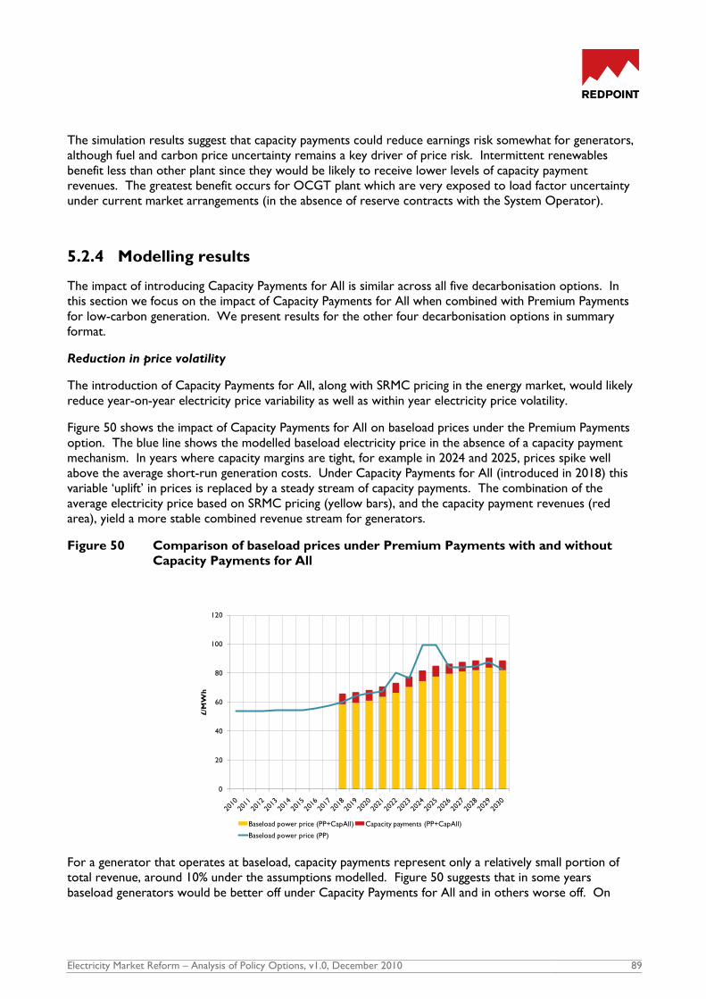
Electricity Market Reform – Analysis of Policy Options, v1.0, December 2010 89
The simulation results suggest that capacity payments could reduce earnings risk somewhat for generators,
although fuel and carbon price uncertainty remains a key driver of price risk. Intermittent renewables
benefit less than other plant since they would be likely to receive lower levels of capacity payment
revenues. The greatest benefit occurs for OCGT plant which are very exposed to load factor uncertainty
under current market arrangements (in the absence of reserve contracts with the System Operator).
5.2.4 Modelling results
The impact of introducing Capacity Payments for All is similar across all five decarbonisation options. In
this section we focus on the impact of Capacity Payments for All when combined with Premium Payments
for low-carbon generation. We present results for the other four decarbonisation options in summary
format.
Reduction in price volatility
The introduction of Capacity Payments for All, along with SRMC pricing in the energy market, would likely
reduce year-on-year electricity price variability as well as within year electricity price volatility.
Figure 50 shows the impact of Capacity Payments for All on baseload prices under the Premium Payments
option. The blue line shows the modelled baseload electricity price in the absence of a capacity payment
mechanism. In years where capacity margins are tight, for example in 2024 and 2025, prices spike well
above the average short-run generation costs. Under Capacity Payments for All (introduced in 2018) this
variable „uplift‟ in prices is replaced by a steady stream of capacity payments. The combination of the
average electricity price based on SRMC pricing (yellow bars), and the capacity payment revenues (red
area), yield a more stable combined revenue stream for generators.
Figure 50 Comparison of baseload prices under Premium Payments with and without
Capacity Payments for All
For a generator that operates at baseload, capacity payments represent only a relatively small portion of
total revenue, around 10% under the assumptions modelled. Figure 50 suggests that in some years
baseload generators would be better off under Capacity Payments for All and in others worse off. On
0
20
40
60
80
100
120
£/M
Wh
Baseload power price (PP+CapAll) Capacity payments (PP+CapAll)
Baseload power price (PP)

Electricity Market Reform – Analysis of Policy Options, v1.0, December 2010 90
average, under the Premium Payments option, total revenues for baseload generators are slightly lower
over the modelling period when Capacity Payments for All are included.
For mid-merit and peaking plant, however, the capacity payments would represent a much larger
component of the overall revenue stream. For example, an older CCGT, which is available for 90% of the
year, would receive capacity payments equivalent to around £55-60/kW/yr. This should be sufficient to
cover annual fixed operating costs providing an incentive for the plant to remain open even when operating
with very low load factors. Hence, for the scheme modelled, average revenues for mid-merit and peaking
plant are likely to be higher, and more certain, when a capacity mechanism is in place.
Impact on security of supply
The main objective of a capacity mechanism is to ensure that there is sufficient generating capacity (and
demand-side response) available to the system to meet an acceptable level of security of supply (which we
have assumed in the modelling is a de-rated capacity margin of 10%). Capacity Payments for All, at the
levels modelled, would likely significantly increase de-rated capacity margins and reduce the risk of
unserved energy.
Figure 51 and Figure 52 show the impact of Capacity Payments for All on de-rated capacity margins and
expected energy unserved for the Premium Payments option. De-rated capacity margins are significantly
higher after 2020 with Capacity Payments for All, and are at or higher than historical levels. As we discuss
below, one of the main contributing factors to the increase in de-rated capacity margins is the extension in
lifetimes of existing coal and gas plant.
Figure 51 De-rated capacity margins under Premium Payments with / without Capacity
Payments for All
The increase in capacity has the impact of reducing the risk that there is not enough supply available to
meet demand, and therefore the risk of energy unserved is apparently very low with Capacity Payments for
All. However, this result does assume that the plant on the system is able to provide the flexibility
required to manage intermittency associated with renewables.
2010 2012 2014 2016 2018 2020 2022 2024 2026 2028 2030
0%
5%
10%
15%
20%
25%
30%
Baseline PP PP+CapAll

Electricity Market Reform – Analysis of Policy Options, v1.0, December 2010 91
Figure 52 Expected Energy Unserved under Premium Payments with / without Capacity
Payments for All
In all policy options modelled, the introduction of Capacity Payments for All leads to increases in de-rated
capacity margins. The impact varies across options and the target objective of keeping de-rated capacity
margins above 10% is not achieved in all cases, as shown in Table 16 below. For example, the de-rated
capacity margin still falls as low as 6.8% under Contracts for Difference. This demonstrates the risk with
priced-based capacity mechanisms – there is no guarantee that a certain security standard will be met,
while in other years they could lead to over-capacity.
Table 16 Minimum de-rated capacity margins 2010-2030
Minimum de-rated capacity margin
Without capacity payments With Capacity Payments
Baseline 5.1% 5.7%
FP 2.4% 9.2%
PP 2.3% 10.2%
CfD 2.2% 6.8%
CPS50 4.6% 10.5%
EPS 5.7% 6.5%
Impact on retirements
Capacity Payments for All would likely lead to the deferral of retirements, particularly of older CCGTs.
Figure 53 and Figure 54 show cumulative plant retirements with and without Capacity Payments for All
under the Premium Payments policy. Capacity payments change the economics for existing plant and
encourage them to stay open longer since annual fixed costs can be covered by the payments. Existing
generators with declining load factors receive higher, more stable revenues under Capacity Payments for
All. In total 8 GW of CCGT and 2 GW of coal is extended by between two and ten years.
2010 2012 2014 2016 2018 2020 2022 2024 2026 2028 2030
0
5
10
15
20
25
30
GW
h
Baseline PP PP+CapAll

Electricity Market Reform – Analysis of Policy Options, v1.0, December 2010 92
Capacity payments may lead to generators changing their decisions surrounding the IED. Within the
modelling, a number of older CCGTs change from LLO to TNP in order to stay open after 2023. The
timing of the announcement surrounding a capacity payment mechanism is therefore important with
respect to decisions generators make surrounding the IED.
Figure 53 Cumulative plant retirements – Premium Payments
Figure 54 Cumulative plant retirements – Premium Payments + Capacity Payments for
All
Impact on new build
The modelling suggests that the introduction of Capacity Payments for All does not necessarily lead to
significantly greater investment in new plant. Premium Payments have been adjusted to reflect lower
wholesale energy market revenues but greater income from capacity payments. Investment in low-carbon
generation is broadly unchanged as a result.
0
5000
10000
15000
20000
25000
30000
35000
40000
45000
2010 2012 2014 2016 2018 2020 2022 2024 2026 2028 2030
MW
Oil
GT & OCGT
Nuclear
Coal
CCGT
0
5000
10000
15000
20000
25000
30000
35000
40000
45000
2010 2012 2014 2016 2018 2020 2022 2024 2026 2028 2030
MW
Oil
GT & OCGT
Nuclear
Coal
CCGT

Electricity Market Reform – Analysis of Policy Options, v1.0, December 2010 93
If low-carbon investment is forthcoming, the targeted de-rated capacity margin can be achieved largely
through lifetime extensions of existing plant68. Figure 55 and Figure 56 show cumulative new build by
technology with and without Capacity Payments for All under the Premium Payments option. The
cumulative amount of new CCGT capacity is only slightly higher by 2025 when capacity payments are
introduced. There is also no investment in new OCGTs. This is because capacity payments turn out just
below the level required to support new OCGT build due to the surplus of existing plant. The modelled
capacity mechanism treats all thermal capacity equally and therefore does not incentivise plant with any
particular technical capabilities. There is therefore a risk with a universal capacity payment mechanism that
the wrong type of capacity is incentivised.
Figure 55 Cumulative new plant build – Premium Payments
Figure 56 Cumulative new plant build – Premium Payments + Capacity Payments for All
68
Although not modelled, there may also be increased demand-side response.
-
10,000
20,000
30,000
40,000
50,000
60,000
70,000
2010 2012 2014 2016 2018 2020 2022 2024 2026 2028 2030
MW
CCGT Unabated Demo Demo CCS
Gas - CCGT with CCS Coal - IGCC with CCS Coal - ASC with FGD & CCS
Nuclear Renewables
-
10,000
20,000
30,000
40,000
50,000
60,000
70,000
2010 2012 2014 2016 2018 2020 2022 2024 2026 2028 2030
MW
CCGT Unabated Demo Demo CCS
Gas - CCGT with CCS Coal - IGCC with CCS Coal - ASC with FGD & CCS
Nuclear Renewables
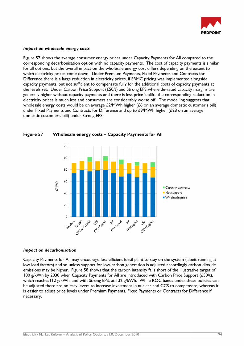
Electricity Market Reform – Analysis of Policy Options, v1.0, December 2010 94
Impact on wholesale energy costs
Figure 57 shows the average consumer energy prices under Capacity Payments for All compared to the
corresponding decarbonisation option with no capacity payments. The cost of capacity payments is similar
for all options, but the overall impact on the wholesale energy cost differs depending on the extent to
which electricity prices come down. Under Premium Payments, Fixed Payments and Contracts for
Difference there is a large reduction in electricity prices, if SRMC pricing was implemented alongside
capacity payments, but not sufficient to compensate fully for the additional costs of capacity payments at
the levels set. Under Carbon Price Support (£50/t) and Strong EPS where de-rated capacity margins are
generally higher without capacity payments and there is less price „uplift‟, the corresponding reduction in
electricity prices is much less and consumers are considerably worse off. The modelling suggests that
wholesale energy costs would be on average £2/MWh higher (£6 on an average domestic customer‟s bill)
under Fixed Payments and Contracts for Difference and up to £9/MWh higher (£28 on an average
domestic customer‟s bill) under Strong EPS.
Figure 57 Wholesale energy costs – Capacity Payments for All
Impact on decarbonisation
Capacity Payments for All may encourage less efficient fossil plant to stay on the system (albeit running at
low load factors) and so unless support for low-carbon generation is adjusted accordingly carbon dioxide
emissions may be higher. Figure 58 shows that the carbon intensity falls short of the illustrative target of
100 g/kWh by 2030 when Capacity Payments for All are introduced with Carbon Price Support (£50/t),
which reaches112 g/kWh, and with Strong EPS, at 132 g/kWh. While ROC bands under these policies can
be adjusted there are no easy levers to increase investment in nuclear and CCS to compensate, whereas it
is easier to adjust price levels under Premium Payments, Fixed Payments or Contracts for Difference if
necessary.
0
20
40
60
80
100
120
£/M
Wh
Capacity payments
Net support
Wholesale price

Electricity Market Reform – Analysis of Policy Options, v1.0, December 2010 95
Figure 58 Annual average carbon dioxide emissions intensity – Capacity Payments for All
Cost benefit analysis
Table 17 shows the cost benefit analysis for the Capacity Payment for All options relative to the respective
decarbonisation options alone. The cost benefit analysis results relative to the Baseline are shown in
Appendix G69.
69
Please note that though Capacity Payments for All are assumed to be introduced in 2018 in the model, the associated benefits and costs are
discounted back to 2010.
2010 2012 2014 2016 2018 2020 2022 2024 2026 2028 2030
0
100
200
300
400
500
600
g/k
Wh
Baseline FP+CapAll PP+CapAll CfD+CapAll CPS50+CapAll EPS+CapAll

Electricity Market Reform – Analysis of Policy Options, v1.0, December 2010 96
Table 17 Cost benefit analysis relative to decarbonisation option
Introducing Capacity Payments for All generally leads to a reduction in net welfare (relative to the
decarbonisation option without capacity payments) since the additional resource costs associated with
having more capacity on the system are greater than the savings in expected energy unserved. However,
this result is critically dependent on assumptions regarding the cost of unserved energy. We have assumed
an average value of lost load (VoLL) of £10,000/MWh.
Under Carbon Price Support (£50/t) and Strong EPS, the inclusion of Capacity Payments for All appears to
lead to an increase in net welfare. However, this is due to the lower investment in low-carbon generation
which results from the lifetime extensions of existing plant and comes at the cost of not achieving the
decarbonisation objectives.
The distributional effects of Capacity Payments for All are much greater than the overall net welfare
impact. Under our modelling assumptions, consumers are worse off with Capacity Payments for All for the
reasons described above. Correspondingly, producers are significantly better off particularly under Carbon
Price Support (£50/t) and Strong EPS.
These results suggest that price based capacity mechanisms could be expensive for consumers. By varying
the level of capacity payments, we have identified that under some decarbonisation options it may be
possible to reduce the level of payment with no loss in security of supply. Under the Fixed Payments
option it is possible to maintain a de-rated capacity margin close to 10% through the combination of early
investment in low-carbon generation and lifetime extensions of existing plant. There is also potential for
greater demand-side response, although this has not been modelled. In this case, a reduction in capacity
payments of 30%, to around £5/MWh of availability, is still sufficient to keep older plant on the system, and
yields the same levels of de-rated capacity margin (although there is an increased risk that new CCGT
investment might not be forthcoming). At this level, the additional cost to consumers from the capacity
payment mechanism would be very small (on the assumption that the electricity prices are based on
SRMCs).
Change in welfare
NPV 2010-2030,
(£m 2009 real)
Carbon Price
Support (£50/t)
& Capacity
Payments For
All
Strong
Emissions
Performance
Standard +
Capacity
Payments For
All
Premium
Payments +
Capacity
Payments For
All
Fixed Payments
+ Capacity
Payments For
All
Contracts for
Difference +
Capacity
Payments For All
Carbon costs -1,828 -2,654 -84 18 1,883
Generation costs -2,754 -3,495 -2,347 -1,287 2,006
Capital costs 7,403 10,257 -2,040 0 -4,446
Unserved energy 192 104 444 434 426
Demand side response 33 20 59 61 49
Change in Net Welfare 3,047 4,232 -3,968 -774 -83
Wholesale price 9,369 732 25,990 27,599 33,199
Low carbon payments -5,346 -4,201 -6,303 -7,915 -7,550
Capacity payments -35,136 -35,120 -35,136 -29,196 -35,099
Unserved energy 192 104 444 434 426
Demand side response 33 20 59 61 49
Change in Consumer Surplus -30,888 -38,465 -14,946 -9,016 -8,976
Wholesale price -9,369 -732 -25,990 -27,599 -33,199
Low carbon support 5,335 4,100 6,341 7,913 7,517
Capacity payments 35,136 35,120 35,136 29,196 35,099
Producer costs 1,900 4,108 -4,471 -1,269 -558
Change in Producer Surplus 33,002 42,596 11,015 8,240 8,859
Net Welfare
Distributional analysis
Consumer
Surplus
Producer Surplus

Electricity Market Reform – Analysis of Policy Options, v1.0, December 2010 97
However, under other options where low-carbon investment comes later, and new thermal capacity is
needed to fill the capacity gap, this lower level of capacity payment would not be sufficient to stimulate
investment. This illustrates the difficulty in setting the correct level for a priced-based universal capacity
mechanism. Volume-based mechanisms, such as capacity auctions, may offer a more cost effective solution
in this respect by helping to reveal the value of different types of capacity.
5.3 Targeted Capacity Tender
5.3.1 Description
The Targeted Capacity Tender differs from Capacity Payments for All in that it would only cover a small
subset of generating plant or demand-side response. Under the Targeted Capacity Tender, a central body,
probably the System Operator, would be responsible for procuring a volume of back-up capacity to meet a
defined security standard. This would in effect be an extension of the System Operator‟s current role in
procuring reserve and other balancing services. The costs of the tendered capacity could be recovered
through Use of System charges.
To fulfil this role the central body would forecast expectations of de-rated capacity margins for a defined
number of years forward. To the extent that the de-rated capacity margin is expected to fall below the
defined security standard it would tender for additional capacity, which could include new generation
capacity, demand-side response or extensions to existing plant that would otherwise be closing on
economic grounds70. Tenders could be run on a rolling annual basis.
Since the de-rated capacity margin includes a capacity credit for wind that is non-zero, a more conservative
approach would be to procure back-up assuming no output from wind plant. This would be an important
consideration when designing the security standard.
The mix of capacity that the central body procures will depend on the System Operator‟s requirements for
flexibility and responsiveness. For example, in order to manage variability in wind output a certain
proportion of the capacity will need to be able to ramp very quickly. Not all existing generating plant will
necessarily be able to meet this requirement.
A very important consideration is the impact of the tendered capacity on electricity prices. If as a result of
the procurement of additional back-up, investors‟ expectations of future electricity prices are dampened,
the policy could become self-defeating with progressively less private investment and a progressively
increasing requirement for back-up. There are broadly two alternatives to mitigate this risk:
to use the back-up capacity only as a „strategic reserve‟ to be deployed as a last resort before
firm load curtailment would occur, which should mean that prices still spike to high levels
when margins become very tight, or
to use the back-up capacity when the electricity price exceeds its utilisation (short-run
operating) cost but to price in the availability fees of the capacity into imbalance charges thus
maintaining signals on parties to cover their peak positions.
70
The tender would need to be designed carefully so as not to create the unintended consequence that plant that would have been available
announce an intention to close in order to be able to participate in the tender.

Electricity Market Reform – Analysis of Policy Options, v1.0, December 2010 98
The latter approach is similar to how the costs of reserve are currently factored into imbalance charging71.
Exactly how this would be done with respect to back-up capacity would be an important design
consideration.
5.3.2 Modelling assumptions
We assume that Targeted Capacity Tenders are introduced when the de-rated capacity margin is forecast
to drop below a required security standard, which we assume to be a 10% de-rated capacity margin. For
simplicity, we assume that the SO has perfect foresight in tendering for the correct amount of capacity
required, and that all tendered capacity is delivered. In reality, there will clearly be uncertainty on both the
supply- and demand-side forecasts in determining the requirement.
Under our approach, the SO tenders for capacity which fulfils certain flexibility and responsiveness
requirements, some of which can be provided by existing plant and some of which would be from new
OCGT plant. We have not modelled the potential role of demand-side response in the tender, although
we recognise that this could fulfil some of the requirement and would have the potential to lower the costs
to consumers.
The tender would be broken down into longer duration and shorter duration contracts. The longer
duration tenders would be necessary to secure investment in new flexible OCGT plant, and we have
assumed 20 year contracts. There is a balance here between providing longer-term certainty for investors
in OCGTs and the risk of stranded assets should de-rated capacity margins subsequently recover. Shorter
contracts could be offered but bidders would likely increase their price so that they could earn their
required return over a shorter period. The shorter duration tenders would be run more frequently and
cover existing plant. We have assumed that both the long and short duration tenders are paid as bid,
although again this is design question.
We have assumed initially that the tendered capacity is used as a strategic reserve, and hence in theory
would not influence price. Hence, consumers would benefit from improved security of supply but not
necessarily from the avoidance of large price spikes associated with very tight capacity margins. We also
consider a variant where the tendered capacity can be used by the System Operator when prices exceed
the utilisation fee for the capacity, with the availability fees priced into the imbalance prices. This approach
would prevent prices peaking to extreme levels but should in theory maintain incentives on parties to
cover their peak positions since the cost of providing peaking capacity should still be reflected in the
market price of electricity.
5.3.3 Modelling results
We have modelled the impact of a Targeted Capacity Tender on one of the decarbonisation options, Fixed
Payments. In this option the de-rated capacity margin falls below 10% in the 2020s. Figure 59 shows the
de-rated margin excluding the tendered capacity, the tendered capacity in each year, and the final de-rated
margin including the tendered capacity.
We assume that part of the forecast capacity shortfall, which peaks at 5.4 GW in 2024, is filled through
long-term tenders for new OCGT capacity, which is also capable of providing a high degree of
responsiveness. Thereafter, more general capacity requirements are met through shorter term tenders,
71
As laid out in the Balancing Services Adjustment Data Methodology (http://www.nationalgrid.com/NR/rdonlyres/C6941419-3742-43A5-B4EE-
3AFB03C324A4/38313/BSADv5_Review1.pdf)

Electricity Market Reform – Analysis of Policy Options, v1.0, December 2010 99
which are filled by extensions of older gas and coal plant that would otherwise have closed. The mix of
long-term and short-term tenders, and the technical specifications for these, would be based on the System
Operator‟s assessment of future system requirements. If the security standard assumed a zero de-rating
factor for wind, the peak requirement for tendered capacity would double to around 10.7 GW.
We assume that in the long-term capacity tenders, the cleared bids cover annual fixed costs as well as
annuitised capital costs (financed over the economic life of the plant), and equate to around £60/kW/yr.
The price received by existing capacity in the short-term tenders is assumed to cover annual fixed costs as
well as a margin over these costs, which equates to around £43/kW/yr.
Figure 59 Impact on capacity margins – Fixed Payments + Targeted Capacity Tender
Figure 60 shows the impact on annual expected energy unserved of the Targeted Capacity Tender on the
Fixed Payments option. The risk to security of supply is significantly reduced, and lower than the Baseline
which is also shown in the graph.
Figure 60 Impact on expected energy unserved – Fixed Payments + Targeted Capacity
Tender
0.0%
5.0%
10.0%
15.0%
20.0%
25.0%
30.0%
2010 2012 2014 2016 2018 2020 2022 2024 2026 2028 2030
0
1
2
3
4
5
6
De
art
ed
marg
in
GW
New OCGT Existing CCGT
Existing Coal Required non-derated capacity, GW
De-rated capacity margin, % De-rated capacity margin excl. Tender, %
2010 2012 2014 2016 2018 2020 2022 2024 2026 2028 2030
0
5
10
15
20
25
30
GW
h
Baseline FP FP+TCT

Electricity Market Reform – Analysis of Policy Options, v1.0, December 2010 100
Figure 61 compares the average wholesale energy costs for the Fixed Payments option with and without a
Targeted Capacity Tender. The Targeted Capacity Tender adds about £0.3/MWh which equates to around
£1 on the average annual domestic consumer bill. This compares to between £2/MWh and £9/MWh under
Capacity Payments for All.
Figure 61 Average consumer electricity price
There is no corresponding benefit in terms of lower wholesale electricity prices if the tendered capacity is
held as a strategic reserve. In the alternative case, where tendered capacity is used by the SO when it is
economic to do so72, and not as a last resort, there could be lower wholesale prices as they would no
longer spike up to £10,000/MWh which we have assumed in the modelling is possible if there is insufficient
supply to meet demand73. If, for example, the tendered capacity was priced into imbalance charges at
£500/MWh, effectively putting a cap on prices at this level, then costs to consumers under Fixed Payments
could on average be lower by about £1.3/MWh with a Targeted Capacity Tender74. However, it is difficult
to draw strong conclusions as to whether a Targeted Capacity Tender could result in savings to customers
without a better understanding of how prices behave under times of system stress, and how the tendered
capacity would be deployed and priced into the market.
Table 18 shows the cost benefit analysis for Fixed Payments + Targeted Capacity Tender, relative to Fixed
Payments. There is a slight reduction in net welfare under the Targeted Capacity Tender since the
additional costs of the tender capacity exceed the savings in unserved energy (given assumptions on value
of lost load).
Consumers are slightly worse off than under Fixed Payments without Targeted Capacity Tender primarily
because the benefit in terms of reduction in total unserved energy is outweighed by the cost of the tender.
72
The term „economic‟ in this context pertains to periods when the SRMC of tendered capacity is lower than the SRMC of the system marginal
plant.
73 As explained in Section 3 there may be reasons why under the current arrangements this may not happen.
74 This figure represents an average over the period 2010-2030 and is derived by calculating the reduction in consumer electricity cost resulting
from imposing a £500/MWh price cap on the wholesale price of electricity. This calculation assumes that there is no change to dispatch or to the distribution of prices below £500/MWh as a result of imposing the price cap.
0
20
40
60
80
100
120
£/M
Wh
Capacity payments
Net support
Wholesale price

Electricity Market Reform – Analysis of Policy Options, v1.0, December 2010 101
Table 18 Cost benefit analysis – Targeted Capacity Tender
5.4 Key messages
The modelling of the Baseline and the decarbonisation options suggested that there are potential risks to
security of supply towards the end of this decade and into the next. These risks result from the possible
suppression of electricity market prices as a consequence of support for low-carbon generation, and the
fact that some of this low-carbon generation is intermittent in nature.
One potential mitigating factor for the security of supply risk is the possible expansion of demand-side
response, enabled by smart meters, other demand side technologies and new customer pricing
propositions encouraging them to shift demand away from peaks. However, some form of capacity
mechanism could be introduced to mitigate this risk further. The analysis suggests that if appropriately
designed, Capacity Payments for All or Targeted Capacity Tenders could result in higher de-rated capacity
margins and lower risks to security of supply, although the outcomes in terms of generation mix could be
quite different under these two different schemes. Many other scheme designs are possible.
The cost benefit analysis suggests that the introduction of a capacity payment mechanism could lead to a
small reduction in net welfare since the additional resource costs are generally higher than the savings from
reduced expected energy unserved. However, this result is highly dependent on the assumptions
surrounding the value of lost load, assumed to be an average £10,000/MWh.
Change in welfare
NPV 2010-2030,
(£m 2009 real)
Fixed Payments
+ Targeted
Capacity Tender
Carbon costs 82
Generation costs -709
Capital costs -470
Unserved energy 404
Demand side response 0
Change in Net Welfare -694
Wholesale price -279
Low carbon payments 39
Capacity payments -1,133
Unserved energy 404
Demand side response 0
Change in Consumer Surplus -969
Wholesale price 279
Low carbon support -37
Capacity payments 1,133
Producer costs -1,098
Change in Producer Surplus 277
Net Welfare
Distributional analysis
Consumer
Surplus
Producer Surplus

Electricity Market Reform – Analysis of Policy Options, v1.0, December 2010 102
5.4.1 Impact of options
The analysis suggests that, if appropriately designed, Capacity Payments for All or Targeted Capacity
Tenders could result in higher de-rated capacity margins and lower risks to security of supply. However,
the outcomes in terms of generation mix could be quite different under these two different schemes.
Table 19 summarises the impact of each relative to the underlying decarbonisation option.
Table 19 Decarbonisation + Capacity Mechanism: Summary metrics
Decarbonisation: As older, higher-emitting plant will tend to stay on the system longer under Capacity
Payments for All, emissions can be somewhat higher as a result, particularly under Carbon Price Support
(£50/t) and Strong EPS where it is more difficult to adjust incentives for low-carbon investment in order to
compensate. The Targeted Capacity Tender, by design, has minimal effect since the back-up capacity would
only be run when required to meet peak system requirements.
Generation mix: Older plant stay on the system longer under Capacity Payments for All, and no new
OCGTs are built. In contrast, new OCGTs are specifically brought on-line, together with some extensions,
under the Targeted Capacity Tender. It may also be possible to target particularly forms of demand-side
response.
Security of supply: The de-rated capacity margin increases significantly under both options. Under a
price-based version of Capacity Payments for All, it can still fluctuate around the target security standard,
although it averages higher due to the stronger incentives to keep existing plant open for longer.
Resource costs: There is some increase in resource costs in most cases, except for Carbon Price Support
(£50/t) and Strong EPS, under which low-carbon investment is somewhat reduced (meaning that
decarbonisation targets are not met).
Resource
costs
Costs to
consumers CBA
Carbon
intensity Cum. CO2
NPV rel. to
baseline
Average
wholesale
energy cost
Net welfare
relative to
Baseline
2030 2010-2030
Ave 2018-
2030
Min 2018-
2030 2010-2030 2010-2030 2010-2030
Baseline No capacity mechanism 207 2973 7.6% 5.1% N/a 91 N/a
Central 100 2377 9.6% 5.7% 7,815 94 -7,706
Capacity Payments for All 132 2472 13.6% 6.5% 3,707 103 -3,474
Central 100 2207 8.8% 4.6% 5,836 95 -5,780
Capacity Payments for All 113 2285 16.0% 10.5% 3,015 101 -2,733
Central 101 2782 7.7% 2.3% 6,471 94 -6,698
Capacity Payments for All 102 2784 16.3% 10.2% 10,942 97 -10,666
Central 101 2599 6.9% 2.4% 3,621 91 -3,846
Capacity Payments for All 101 2596 14.8% 9.2% 4,890 93 -4,620
Targeted Tender Capacity 101 2591 6.9% 2.4% 4,719 92 -4,540
Central 98 2606 6.7% 2.2% 3,678 91 -3,965
Capacity Payments for All 99 2531 10.1% 6.8% 4,236 93 -4,049
Strong EPS
Carbon Price
Support
Premium
Payments
Fixed Payments
Contracts for
Difference
Capacity margin
Decarbonisation
optionCapacity mechanism
Decarbonisation Security of supply
Electricity Market Reform – Analysis of Policy Options, v1.0, December 2010 103
Costs to consumers: Under Capacity Payments for All, costs to consumers increase (by between 6 and
£28 per year on average over the period 2010-2030 for a domestic customer) as the reduction in
electricity prices is less than the capacity payments to generators. However, assuming the „uplift‟ in prices
is subsequently avoided, consumers should benefit from reduced volatility in prices associated with system
tightness. The cost increase is much smaller under the Targeted Capacity Tender, on average around £1
per year for a domestic consumer. If the tendered capacity is utilised when economic to do so (ie, not held
as a strategic reserve) and appropriately priced into the market, extreme price spikes could be avoided, and
it is possible that there could be cost savings for consumers.
Generator rents: There is a risk of rents for generators under Capacity Payments for All depending on
the level set, and whether prices in the bilateral market subsequently SRMC pricing. The risk is lower
under the Targeted Capacity Tender.
5.4.2 Risks of options
Incorrect levels: In both cases, it will be difficult to evaluate the appropriate security standard,
particularly as the penetration of intermittent renewables increases. For the price-based approach, an
appropriate benchmark „cost of capacity‟ will also be required. Getting these levels wrong could lead either
to higher costs for consumers, or result in a lower level of security of supply than intended.
Forecast uncertainty: The volume-based approach requires the tendering body to forecast both demand
and the supply position (including demand-side response) over a number of years forward. Both of these
are uncertain, meaning that the resulting tendered volumes may correspondingly be too high or too low.
In practice it is likely that the central entity tasked with ensuring the security standard will err on the side
of higher volumes (to ensure a defined target is met) as it will be challenging to create incentives that
reflect the risk of higher costs to consumers in this case.
Displacement of investment: There is a risk, despite the intended design of the mechanism, that
tendering for peak capacity may displace investment that would otherwise have taken place, due to an
anticipated effect on prices. This may be particularly true for demand-side response, and other smaller
scale innovative technologies, as although in theory this could be eligible for payments, in practice
monitoring and administrative requirements may be relatively much more onerous. There is a further risk
that existing plant may announce an intention to close earlier in order to increase the requirement for
tendered capacity, and make themselves eligible to participate. The combination of this and displaced
investment could result in an unintended consequence of a progressively expanding role for a central buyer
of capacity.
Flexibility requirements: The price-based Capacity Payments for All may lead to a mix of plant that,
while nominally providing a required level of total capacity, does not provide the flexibility required to
manage the fluctuation in demand and intermittent renewable output. This can be addressed with the
Targeted Capacity Tender option by tendering for different tranches of capacity with specific technical
requirements.
Wholesale price uplift: The principle of Capacity Payments for All is that this new revenue stream will
cover the capital and fixed costs of low load factor plant, such that these plant are economic without the
need for significant price „uplift‟ above the system SRMC. With this in place, any remaining „uplift‟ creates
rents to generators with no benefit to consumers. However, it is difficult to see how this could be
monitored and controlled in a bilateral market.
Interconnected markets: Other than the Irish SEM, none of GB‟s neighbouring markets have capacity
payments. The design of the scheme would need to consider carefully the impact of greater future

Electricity Market Reform – Analysis of Policy Options, v1.0, December 2010 104
interconnection (for example the 1 GW BritNed cable in 2012) and plans for market coupling. Greater
market integration and regional harmonisation may become more difficult.
5.4.3 Implementation issues
Timing: As discussed above, the introduction of capacity payments could change the economics around
plant retirement. For older CCGTs, this could lead to different decisions with regard to their choices
under the IED. As a result, the timing of the announcement and implementation of a capacity payment
scheme should take this into account.
Administration: A Targeted Capacity Tender would be a natural extension of the System Operator‟s
current reserve procurement function. Capacity Payments for All would represent a separate revenue
stream for generators, and an entity will need to manage the associated settlements, cashflows and credit,
as well as the recovery of the costs. It may be noted that the processes would be equivalent to availability
payments for low-carbon generation, and hence there would be efficiency in combining these processes.
Demand side: There is significant potential for the demand side of the market to provide response that
would help the dynamic balancing of the system and reduce overall capacity requirements. It is likely that
provision of this response will involve up front capital investments in instrumentation and communications
technology to ensure an appropriate level of control for the System Operator. It is therefore important
that careful consideration is given in the design of any capacity payment mechanism (either Capacity
Payments for All or Targeted Capacity Tender) to ensure that demand side investments can compete on an
equitable basis with both new generation investments and the life-extension of existing generation assets.
In particular, the timescales and granularity of the capacity „service‟ requirements must be consistent with
making investments in demand response capability.
Monitoring: As noted above, introducing Capacity Payments for All could require monitoring of market
prices to mitigate against the risk of continuing price „uplift‟. While a market-level indication of this could
be generated by comparing outturn spot prices to those theoretically predicted from modelling, it is
extremely difficult to envisage a method which could be used to connect this to the behaviour of specific
market participants without drastically changing the market arrangements, or imposing very burdensome
regulation on trading activities.
5.4.4 Summary
Capacity Payments for All
Capacity Payments for All would be likely to lead to improved capacity margins and reduce the risks to
security of supply. It could reduce price volatility and increase investor confidence in developing new plant,
particularly in CCGTs, that may no longer be able to guarantee baseload operation with high levels of low-
carbon generation deployment.
However, it would be difficult to establish the correct level to set capacity payments at, and a universal
scheme may not deliver an appropriate generation mix to provide the flexibility needed in a system with
increasing proportions of intermittent renewables. With additional support for low-carbon investment, the
required de-rated capacity margins could be achieved predominantly through extensions of existing coal
and gas plant on the system. This would require capacity payments to be set at a relatively low level,
sufficient to cover the annual fixed costs of these assets and any capital expenditure required in order to
extend their lifetime. However, this older plant may not be sufficiently flexible. To attract more flexible
back-up plant, such as new OCGTs, capacity payments would need to be set at a higher level. However,

Electricity Market Reform – Analysis of Policy Options, v1.0, December 2010 105
this could lead to windfalls for existing plant. In addition, there is a significant risk that generators are over-
remunerated should electricity prices not fall on the introduction of the scheme, and any form of price
regulation would be difficult with current trading arrangements. Similarly, compatibility with
interconnected markets could be an issue, especially with increasing regional harmonisation.
For these reasons, designing an appropriate administered scheme becomes very difficult. Implementing a
quantity-based capacity auction could address some of these issues and would aid price discovery, and the
specification for the auctions could be more tightly defined to deliver the requisite flexibility.
Targeted Capacity Tender
The main benefit of the Targeted Capacity Tender relative to the Capacity Payments for All is that it allows
for specific tranches of back-up to meet different technical requirements, particularly around flexibility.
Through direct tendering, it removes the risk of windfalls for generators. It can act as an insurance policy
and be implemented when it is needed, and therefore would be less disruptive to current market
arrangements.
Nevertheless, forecast uncertainty will still represent a challenge, as will the risk that the tendered capacity
could undermine private investment, and encourage existing plant to announce earlier closure, thus
exacerbating a forecast capacity shortage.

Electricity Market Reform – Analysis of Policy Options, v1.0, December 2010 106
6 Combination Packages 6.1 Packages considered
In this section we explore packages of options that combine Carbon Price Support set at a lower level with
other policy options. The packages that we consider are:
Premium Payments with Carbon Price Support (£30/t)
Premium Payments, Carbon Price Support (£30/t) and Targeted Capacity Tenders
Fixed Payments, Carbon Price Support (£30/t) and Targeted Capacity Tenders, and
Contracts for Difference, Carbon Price Support (£30/t) and Targeted Capacity Tenders.
We also include a High Demand sensitivity on two of the combination packages in Appendix B.
The level of Carbon Price Support assumed in these combination packages rises less rapidly than that
considered for the stand-alone Carbon Price Support (£50/t) option. It reaches £30/t by 2020 (compared
to £50/t), before hitting the same level of £70/t by 2030, as shown in Figure 62 below. This scenario is
consistent with the mid-range of illustrative scenarios presented in HM Treasury‟s Carbon Price Support
consultation.
Figure 62 Carbon Price Support (£30/t)
When Carbon Price Support (£30/t) is combined with Fixed Payments we assume that the utilisation fee
(for CCS plant) is automatically adjusted for a higher carbon cost75 through the input cost indexation term,
but that the availability fees remain unchanged. Likewise, there would be no change to the premia under
Contracts for Difference. Hence, under these two combinations, adding Carbon Price Support (£30/t) has
no impact on the amount of low-carbon investment that is projected in the modelling.
Investors are exposed to electricity prices under Premium Payments, and hence we assume that premia can
be adjusted downwards to reflect higher expectations of electricity prices when Carbon Price Support
(£30/t) is combined with this option.
75
We assume a 90% capture rate for CCS.
2010 2012 2014 2016 2018 2020 2022 2024 2026 2028 2030
0
10
20
30
40
50
60
70
80
£/t
on
ne
CPS30 Support level CPS50 Support level Baseline carbon price

Electricity Market Reform – Analysis of Policy Options, v1.0, December 2010 107
We assume that a Targeted EPS as described in Section 4.2.5 is also included in these combination
packages.
6.2 Modelling results
We compare the results of modelling the combination packages with each underlying decarbonisation
option (Fixed Payments, Premium Payments, or Contracts for Difference). We separate the effects of the
two additional policies (Carbon Price Support (£30/t) and Targeted Capacity Tender) in order to answer
the following questions:
What is the impact of combining Carbon Price Support (£30/t) with other decarbonisation
options?
What is the impact of a Targeted Capacity Tender on these combinations?
6.2.1 Plant mix
The impact of Carbon Price Support (£30/t) on low-carbon investment varies depending on the option it is
combined with. Under Fixed Payments and Contracts for Difference, investors in low-carbon generation
have limited exposure to electricity prices and hence the modelled impact of Carbon Price Support (£30/t)
on investment is minimal. As shown in Table 20, the timing and volumes of new nuclear and CCS capacity
are similar to the underlying decarbonisation option76.
The pattern of low-carbon build does, however, change when Carbon Price Support (£30/t) is combined
with Premium Payments. With Carbon Price Support (£30/t), premia can be reduced while still achieving
the targeted emissions intensity by 2030. As costs come down, Carbon Price Support (£30/t) is sufficient
alone to stimulate new nuclear and the premium can be reduced to zero. With more nuclear investment,
less CCS is required to meet the same decarbonisation level and we have reduced premia for CCS so that
the 2030 carbon intensity of 100 g/kWh is maintained. This is consistent with the analysis of the Carbon
Price Support (£50/t) option which suggested that Carbon Price Support (a technology neutral instrument)
may tend to favour cheaper and more mature technologies, relative to more targeted support options such
as Premium Payments.
Table 20 Timing and capacity of Nuclear and CCS investment77
PP FP CfD
PP+
CPS30
PP+
CPS30+
TCT
FP+
CPS30+
TCT
CfD+
CPS30+
TCT
Year of first new
nuclear 2023 2019 2019 2023 2023 2019 2019
New nuclear capacity
(2030) 9.6 GW 9.6 GW 11.2 GW 12.8 GW 12.8 GW 9.6 GW 9.6 GW
New CCS capacity
(2030)1 7.0 GW 7.0 GW 5.5 GW 2.0 GW 2.0 GW 7.0 GW 7.0 GW
76
Note that under Contracts for Difference, adding Carbon Price Support (£30/t) and Targeted Capacity Tender results in a fall in nuclear capacity by 2030 with a corresponding increase in CCS capacity. This results from lumpiness in the setting of CfD strike prices in the model and we do not
believe this result to be significant.
77 Note that new CCS capacity excludes retrofitted capacity.

Electricity Market Reform – Analysis of Policy Options, v1.0, December 2010 108
The inclusion of Carbon Price Support (£30/t) within the combination packages has little impact on
investment in CCGT. The inclusion of Carbon Price Support (£30/t) does, however, accelerate the closure
of some coal plant under the combination packages.
The inclusion of a Targeted Capacity Tender within the packages results in additional OCGT capacity on
the system and lifetime extensions for some coal and gas plant, as shown below.
6.2.2 Carbon dioxide emissions
Figure 63 shows annual carbon intensity with and without Carbon Price Support (£30/t) under the
Premium Payments combinations. The difference in emissions intensity is small before 2020, suggesting this
trajectory of Carbon Price Support would not lead to significant coal to gas switching under DECC‟s
Central assumptions before 2020. As the support level rises above £30/t after 2020, coal to gas switching
starts to occur, and with more rapid deployment of nuclear, carbon emissions intensity falls more rapidly
than under the Premium Payments alone. A further effect is that CCS plant operate at higher load factors
given their greater competitiveness with unabated fossil plant.
The inclusion of Targeted Capacity Tender has little additional impact on carbon dioxide emissions. The
capacity operates rarely and therefore has little impact on overall emissions intensity.
Figure 63 Emissions intensity – Premium Payments combination packages
Figure 64 show the cumulative emissions over the period 2010-2030 for the Premium Payments
combination packages. The inclusion of Carbon Price Support (£30/t) results in a reduction in carbon
dioxide emissions over the period of 125 Mt or 4%. This result is sensitive to assumptions on coal and gas
prices.
2010 2012 2014 2016 2018 2020 2022 2024 2026 2028 2030
0
100
200
300
400
500
600
g/k
Wh
PP PP+CPS30 PP+CPS30+TCT

Electricity Market Reform – Analysis of Policy Options, v1.0, December 2010 109
Figure 64 Cumulative carbon dioxide emissions – Premium Payments combination
packages
Figure 65 shows carbon intensity when Carbon Price Support (£30/t) is combined with Fixed Payments or
Contracts for Difference. As for Premium Payments (above) there is little impact until after 2020 when the
carbon price reaches a level high enough to incentivise significant coal to gas switching. The additional
impact of CCS plant operating at higher load factors also reduces emissions in the mid 2020s. However,
unlike under the Premium Payments combinations, there is no impact in terms of accelerated low-carbon
investment.
Again, the inclusion of Targeted Capacity Tender has little additional impact on carbon dioxide emissions.
Figure 65 Emissions intensity – Fixed Payments and Contracts for Difference combination
packages
Figure 66 shows the cumulative emissions over the period 2010-2030 for the Fixed Payments and Contract
for Difference combination packages. The inclusion of Carbon Price Support (£30/t) results in a reduction
in carbon dioxide emissions over the period of 100 to 105 Mt or 4%.
2010 2012 2014 2016 2018 2020 2022 2024 2026 2028 2030
0
500
1000
1500
2000
2500
3000
3500
mtC
O2
PP PP+CPS30 PP+CPS30+TCT
2010 2012 2014 2016 2018 2020 2022 2024 2026 2028 2030
0
100
200
300
400
500
600
g/k
Wh
FP CfD
FP+CPS30+TCT CfD+CPS30+TCT

Electricity Market Reform – Analysis of Policy Options, v1.0, December 2010 110
Figure 66 Cumulative carbon dioxide emissions – Premium Payments combination
packages
6.2.3 Security of supply
Figure 67 shows the de-rated capacity margins under each of the combination packages prior to the
inclusion of a Targeted Capacity Tender. As in the stand-alone options there appears to be a material risk
to security of supply after 2018. The lower trajectory of the Carbon Price Support (£30/t) does not result
in earlier retirements of coal plant to the same extent as Carbon Price Support (£50/t), but there is also
less new CCGT investment as a consequence.
Figure 67 De-rated capacity margins – Combination packages without Targeted Capacity
Tender
Figure 68 shows the required volumes of tendered capacity to meet at least a 10% de-rated capacity margin
under each of the combination packages. The requirement peaks at 5.5 GW under the Fixed Payments +
Carbon Price Support (£30/t) combination. (A further 5 GW would be required if the security standard
was based on a zero capacity credit for wind.)
2010 2012 2014 2016 2018 2020 2022 2024 2026 2028 2030
0
500
1000
1500
2000
2500
3000
3500
mtC
O2
FP CfD FP+CPS30+TCT CfD+CPS30+TCT
2010 2012 2014 2016 2018 2020 2022 2024 2026 2028 2030
0%
5%
10%
15%
20%
25%
30%
Baseline FP PP CfD FP+CPS30 PP+CPS30 CfD+CPS30

Electricity Market Reform – Analysis of Policy Options, v1.0, December 2010 111
Figure 68 Tendered capacity and impact on de-rated capacity margins margins –
Combination packages with Targeted Capacity Tender
6.2.4 Electricity prices
Figure 69 shows the annual average baseload electricity prices from the modelling under the combination
packages and the corresponding decarbonisation options. Prices are generally higher in the near to
medium term under the combination packages compared to the corresponding decarbonisation options
due to the effect of Carbon Price Support. The Premium Payments + Carbon Price Support (£30/t)
package shows a different pattern of electricity prices through the 2020s as compared to Premium
Payments, due to differences in de-rated capacity margins over this period.
0.0%
5.0%
10.0%
15.0%
20.0%
25.0%
30.0%
2010 2012 2014 2016 2018 2020 2022 2024 2026 2028 2030
0
1
2
3
4
5
6
De
rate
d m
arg
in
GW
OCGT Gas
Coal Required non-derated capacity, GW
Derated capacity margin % Derated margin excl. Tender capacity
0.0%
5.0%
10.0%
15.0%
20.0%
25.0%
30.0%
2010 2012 2014 2016 2018 2020 2022 2024 2026 2028 2030
0
1
2
3
4
5
6
De
rate
d m
arg
in
GW
OCGT Gas
Coal Required non-derated capacity, GW
Derated capacity margin % Derated margin excl. Tender capacity
0.0%
5.0%
10.0%
15.0%
20.0%
25.0%
30.0%
2010 2012 2014 2016 2018 2020 2022 2024 2026 2028 2030
0
1
2
3
4
5
6
De
rate
d m
arg
in
GW
OCGT Gas
Coal Required non-derated capacity, GW
Derated capacity margin % Derated margin excl. Tender capacity
Contracts for Difference + Carbon Price
Support + Targeted Capacity Tender
Fixed Payments + Carbon Price Support +
Targeted Capacity Tender
Premium Payments + Carbon Price
Support + Targeted Capacity Tender

Electricity Market Reform – Analysis of Policy Options, v1.0, December 2010 112
Figure 69 Annual average baseload electricity prices – Combination packages
6.2.5 Wholesale energy costs
Figure 70 shows a comparison of wholesale energy costs for the combination packages relative to the
underlying decarbonisation options. The combination packages are generally more expensive for
consumers, mainly as a result of the higher electricity prices resulting from Carbon Price Support. Under
Fixed Payments and Contracts for Difference, the consumer energy price is on average £2.40/MWh higher
over the period 2010 to 2030, corresponding to an extra £8 per year on the average domestic consumer
bill. Under Premium Payments + Carbon Price Support (£30/t) the higher electricity prices are offset by
the lower premium payments that are required to reach the same level of decarbonisation.
The Targeted Capacity Tender has a very small impact on consumer energy prices because of the relatively
small volumes of capacity involved. The cost impact is an average of £0.26/MWh.
Figure 70 Wholesale energy costs – Combination packages
2010 2012 2014 2016 2018 2020 2022 2024 2026 2028 2030
0
20
40
60
80
100
120
£/M
Wh
Baseline FP PP CfD
FP+CPS30+TCT PP+CPS30+TCT CfD+CPS30+TCT
0
20
40
60
80
100
£/M
Wh
Wholesale price Net support Capacity tender

Electricity Market Reform – Analysis of Policy Options, v1.0, December 2010 113
6.2.6 Cost benefit analysis
Table 21 shows the cost benefit analysis for the combination packages, relative to their respective
decarbonisation option.
Table 21 Cost benefit analysis – combination packages (relative to decarbonisation
option)
The combination packages lead to slightly lower net welfare when associated with Fixed Payments and
Contracts for Difference. This is the due to the distortion of dispatch economics towards more expensive
fuels as a result of Carbon Price Support and the fact that the cost of the tendered capacity is greater than
the assumed savings in the cost of unserved energy. The improvement in net welfare when Carbon Price
Support (£30/t) is combined with Premium Payments results from the replacement of more expensive CCS
with cheaper nuclear plant.
Consumer surplus falls under the combination packages because Carbon Price Support increases wholesale
prices, which feed through to higher bills for consumers. In the case of Premium Payments this is largely
offset by a reduction in low-carbon payment levels, but less so under Fixed Payments and Contracts for
Difference. There are additional costs for consumers associated with the Targeted Capacity Tender,
however these are relatively small.
Under the Premium Payments combinations, producer surplus is lower. Producers benefit from higher
wholesale prices. However, fossil generators are exposed to the costs of Carbon Price Support, and low-
carbon generators receive lower payments. Under Fixed Payments, producers appear collectively better
off since the increase in wholesale prices is not offset by a reduction in low-carbon support to the same
extent.
Change in welfare
NPV 2010-2030,
(£m 2009 real)
Premium
Payments +
Carbon Price
Support (£30/t)
Premium
Payments +
Carbon Price
Support (£30/t) +
Targeted
Capacity Tender
Fixed Payments
+ Carbon Price
Support (£30/t) +
Targeted
Capacity Tender
Contracts for
Difference +
Carbon Price
Support (£30/t) +
Targeted
Capacity Tender
Carbon costs 2,650 2,599 1,970 1,879
Generation costs -21 -523 -2,784 -3,135
Capital costs 1,574 1,077 -315 132
Unserved energy 128 406 404 463
Demand side response 6 7 2 5
Change in Net Welfare 4,336 3,565 -724 -657
Wholesale price -13,457 -13,470 -17,484 -16,763
Low carbon payments 11,867 11,866 4,399 6,976
Capacity payments 0 -1,176 -1,125 -1,169
Unserved energy 128 406 404 463
Demand side response 6 7 2 5
Change in Consumer Surplus -1,456 -2,367 -13,804 -10,488
Wholesale price 13,457 13,470 17,484 16,763
Low carbon support -11,900 -11,900 -4,336 -6,940
Capacity payments 0 1,176 1,125 1,169
Producer costs -6,678 -7,736 -11,026 -11,059
Change in Producer Surplus -5,121 -4,990 3,247 -68
Net Welfare
Distributional analysis
Consumer
Surplus
Producer Surplus

Electricity Market Reform – Analysis of Policy Options, v1.0, December 2010 114
6.3 Key messages
6.3.1 Impact of options
Adding Carbon Price Support (£30/t) to Fixed Payments and Contracts for Difference makes little
difference in terms of low-carbon investment, but does reduce emissions by encouraging coal to gas
switching and helps to ensure that CCS plant runs ahead of unabated plant. By increasing electricity prices
it could, however, lead to higher costs to consumers.
The rationale for combining Carbon Price Support (£30/t) and Premium Payments is perhaps stronger. It
allows the level of premia to be reduced, saving consumers money if carbon prices subsequently rise, and
makes the Premium Payments option more robust to lower outturn carbon prices. It also allows the
market to play a greater role in determining the future generation mix which could lead to a lower cost
outcome.
Decarbonisation: Combining Carbon Price Support (£30/t) with other decarbonisation options is likely
to lead to lower cumulative emissions to 2030 by encouraging coal to gas switching, and making CCS plant
more competitive with unabated fossil plant. Low-carbon investment would be directly affected in
combination with Premium Payments, and the impact would depend on how premia are adjusted to
account for higher anticipated electricity prices. Adding Carbon Price Support (£30/t) to Premium
Payments would also make the package more robust to uncertain carbon prices. However, the
effectiveness of the Premium Payments package in driving low-carbon investment would still be at risk from
lower gas prices. This risk does not occur under the Fixed Payments and Contracts for Difference
combinations. The impact of Targeted Capacity Tenders within these packages on carbon dioxide
emissions would be minimal given the plant would be run relatively infrequently.
Generation mix: Carbon Price Support (£30/t) is likely to have little direct impact on low-carbon
investment when combined with Fixed Payments and Contracts for Difference, but may change the pattern
of investment under Premium Payments. It may be that the Carbon Price Support (£30/t) alone is sufficient
to promote investment in cheaper technologies, and this may favour nuclear, reducing the requirement to
support CCS to meet the same emissions intensity in 2030. The Targeted Capacity Tender would result in
more flexible back-up capacity being held on the system.
Security of supply: The inclusion of the option for Targeted Capacity Tenders should reduce the risk to
security of supply.
Resource costs: There are additional costs associated with the Targeted Capacity Tender. The inclusion
of Carbon Price Support (£30/t) would also increase generation costs by more than the savings in carbon
dioxide emissions (valued at the EUA price). However, in combination with Premium Payments, Carbon
Price Support (£30/t) may lead to a cheaper generation mix which could result in savings in resource costs.
Costs to consumers: In general the inclusion of Carbon Price Support (£30/t) and Targeted Capacity
Tenders within the combination packages increases the costs to consumers. Under Fixed Payments and
Contracts for Difference, these increases average around £2.4/MWh or £8 per year for an average
domestic consumer mainly as the result of higher electricity prices. With Premium Payments the increases
in wholesale prices are largely offset by reductions in support payments, and the additional costs to
consumers are relatively small.
Generator rents: Generators benefit from higher electricity prices when Carbon Price Support (£30/t) is
included in the combination packages, but for fossil generators there are greater carbon costs. Hence,
there are winners and losers. The scaling back of payments to low-carbon generators under Premium
Payments means that generators are collectively worse off under the combination package. However,
under Fixed Payments levels remain unchanged, and hence collectively generators appear better off under

Electricity Market Reform – Analysis of Policy Options, v1.0, December 2010 115
the combination package. In the case of the combination package under Contracts for Difference, welfare
of generators is almost completely unchanged when Carbon Price Support (£30/t) and Targeted Capacity
Tender are included.
6.3.2 Risk of options
The risks associated with the combination packages are similar to those outlined for the individual options
in Sections 4 and 5.
Adopting a lower level of Carbon Price Support (£30/t) does, however, reduce some of the risks related to
rents for existing low-carbon generators and higher costs to consumers in the near term when compared
to Carbon Price Support (£50/t).
Combining Carbon Price Support (£30/t) with Premium Payments helps to reduce the risk that lower than
expected EUA prices result in decarbonisation objectives being missed. Hence, payment levels can be set
with more confidence. There is little long-term benefit of combining Carbon Price Support (£30/t) with
Fixed Payments and Contracts for Difference in terms of greater certainty in low-carbon investment.
However, its introduction, which could be relatively quick, may enhance investor confidence prior to the
establishment of the new low-carbon support arrangements, thus reducing the risk of an investment hiatus.
The benefits in terms of reduced emissions from coal to gas switching under this package need to be
weighed up against the risks of higher costs to consumers, and the risks of unintended consequences such
as the distortion of electricity prices relative to interconnected markets.
Finally, the combination packages would be inherently more complex with greater implementation risks and
risks of further unintended consequences.
6.3.3 Implementation issues
The implementation issues identified for the individual options in Sections 4 and 5 would be similar for the
combination packages, although the interactions between options would also need to be carefully
considered, a good example being the interaction between the level of Carbon Price Support and Premium
Payments levels in that package. Similarly, the levels of strike prices for Contracts for Difference and the
levels of premium payments would be rebalanced, most likely reducing the net cashflow from the
Government to generators.

Electricity Market Reform – Analysis of Policy Options, v1.0, December 2010 116
7 Conclusions
The analysis suggests that the societal costs of delivering the required levels of decarbonisation differ
between the options due to the impact on financing, and the extent to which the Government may target
different technology mixes. However, these differences are relatively small, equivalent to about 1% of the
total wholesale cost of electricity between 2010 and 2030. Where the options differ more markedly is in
their impact on customers, their robustness to key uncertainties, the complexity of implementation and
consequences for the electricity market as a whole.
Fixed Payments or Contracts for Difference (in conjunction with a Targeted EPS) could deliver the best
value for customers and be the most robust to long-term uncertainties around fuel and EUA prices. The
key risks with these approaches are that they depend on Government being able to set prices and target
volumes appropriately, and that they represent a significant departure from current arrangements, with
longer term consequences for the operation of the market. They would be more costly and time
consuming to implement, and the transition would have to be effectively managed to minimise a potentially
significant hiatus in near term investments. The inclusion of Carbon Price Support (£30/t) within the
package may mitigate this latter risk to some extent.
The Premium Payments option would involve less implementation complexity but would be less robust to
long-term uncertainties. If this route is adopted, there appear to be advantages in combining it with
Carbon Price Support (£30/t) since this would make it more robust and potentially cheaper for consumers
than either option by itself. Establishing the appropriate level to set premia remains a challenge however,
given the uncertainty in future gas prices.
The Fixed Payments and Contracts for Difference approaches clearly place more reliance on Government
intervention and central management (with a corresponding transfer of risks from investors), relative to the
Premium Payments approaches, which have less impact on the market overall. This choice is likely to be
strongly influenced by the trade off between longer term certainty in the generation mix versus risks
associated with Government decision-making under uncertainty and information asymmetry, disruption to
current market arrangements and near-term investment.
Finally, the risks to security of supply appear material but uncertain and an insurance policy may be needed.
Retaining the option to include a Targeted Capacity Tender within the policy package appears to offer a
cost-effective mechanism for achieving this and has the potential to stimulate new sources of flexibility.
However, there are many detailed design challenges that will need to be addressed.

Electricity Market Reform – Analysis of Policy Options, v1.0, December 2010 117
A Scenario and sensitivity name
abbreviations
Full name Abbreviation
Carbon Price Support (£50/t) CPS50
Strong Emissions Performance Standard EPS
Premium Payments PP
Fixed Payments FP
Contracts for Difference CfD
Baseline - Low Gas Baseline-LG
Baseline - High Gas Baseline-HG
Baseline - Low Carbon Baseline-LC
Carbon Price Support (£50/t) - Low Gas CPS50-LG
Carbon Price Support (£50/t) - High Gas CPS50-HG
Carbon Price Support (£50/t) - Low Carbon CPS50-LC
Carbon Price Support (£50/t) - Low Investor Confidence CPS50-LowConf
EPS - Low Gas EPS-LG
EPS - High Gas EPS-HG
EPS - Low Carbon EPS-LC
Premium Payments - Low Gas PP-LG
Premium Payments - High Gas PP-HG
Premium Payments - Low Carbon PP-LC
Fixed Payments - Low Gas FP-LG
Fixed Payments - High Gas FP-HG
Fixed Payments - Low Carbon FP-LC
CfDs - Low Gas CfD-LG
CfDs - High Gas CfD-HG
CfDs - Low Carbon CfD-LC
Carbon Price Support (£50/t) & Capacity Payments For All CPS50+CapAll
Strong Emissions Performance Standard + Capacity Payments For All EPS+CapAll
Premium Payments + Capacity Payments For All PP+CapAll
Fixed Payments + Capacity Payments For All FP+CapAll
Contracts for Difference + Capacity Payments For All CfD+CapAll
Premium payments & low capacity payments PP+CapAll(Low)
Fixed Payments + Targeted Capacity Tender FP+TCT
Premium Payments + Carbon Price Support (£30/t) PP+CPS30
Premium Payments + Carbon Price Support (£30/t) + Targeted Capacity Tender PP+CPS30+TCT
Fixed Payments + Carbon Price Support (£30/t) + Targeted Capacity Tender FP+CPS30+TCT
Contracts for Difference + Carbon Price Support (£30/t) + Targeted Capacity Tender CfD+CPS30+TCT
Baseline - High Demand Baseline-HD
Premium Payments + Carbon Price Support (£30/t) + Targeted Capacity Tender - High
Demand
PP+CPS30+TCT-HD
Contracts for Difference + Carbon Price Support (£30/t) + Targeted Capacity Tender -
High Demand
CfD+CPS30+TCT-HD

Electricity Market Reform – Analysis of Policy Options, v1.0, December 2010 118
B High Demand Sensitivity
DECC requested that we explore the sensitivity of the results under higher demand assumptions for the
following two combination packages:
• Contracts for Difference + Carbon Price Support (£30/t) + Targeted Capacity Tender, and
• Premium Payments + Carbon Price Support (£30/t) + Targeted Capacity Tender.
We also have re-run the Baseline under the High Demand sensitivity to provide a comparison for the
policy packages. We present the results in this Appendix.
Assumptions
The assumptions for growth in annual demand for the purposes of these sensitivities are based on a
demand scenario provided to us by the CCC, which represents a greater degree of electrification of the
heating and transport sectors. Peak demand is assumed to grow at 60% of the rate of growth of annual
demand, on the assumption that the additional demand growth would be focused in off-peak periods.
Figure 71 Annual and peak demand – High Demand Sensitivity
For the High Demand sensitivity under the Baseline, RO banding is adjusted to achieve 29% renewable
generation by 2020 and 35% by 2030. In capacity terms this is therefore a higher level of renewables
deployment than under the Central Demand assumptions. For the combination packages, CfD strike prices
and premia levels are adjusted so as to achieve the same renewable generation targets but also to achieve a
carbon dioxide emissions intensity of the electricity system of 100 g/kWh by 203078. In general this means
78
Note that would represent a higher level of decarbonisation for the energy sector as a whole than under Central assumptions since the
additional electrification would be displacing consumption of fossil fuels in other sectors.
0
10
20
30
40
50
60
70
80
90
2010 2012 2014 2016 2018 2020 2022 2024 2026 2028 2030
0
100
200
300
400
500
600P
eak
de
man
d (
GW
)
An
nu
al
de
man
d (
TW
h)
Annual demand - HD Annual demand - Central
Peak demand - HD Peak demand - Central

Electricity Market Reform – Analysis of Policy Options, v1.0, December 2010 119
increasing payment levels in order to stimulate greater low-carbon investment. It is assumed that investors
have visibility of future demand growth79 and are thus able to adjust their investment plans accordingly.
Carbon dioxide emissions
Figure 72 shows the carbon emissions intensity for the generation sector for the Baseline and combination
packages under the High Demand sensitivity and corresponding packages under Central Demand
assumptions. In general, faster demand growth results in a more rapid reduction in emissions intensity
because much of the extra generation comes from low-carbon sources.
Figure 72 Carbon emissions intensity – High Demand Sensitivity
However, in absolute terms carbon dioxide emissions from the generation sector are higher under the
High Demand sensitivity, as more fossil fuel generation is also required to meet the higher demand, as
shown in Figure 73. However, it would be expected that this would be offset by savings elsewhere in the
energy system from less fossil fuel usage as a result of greater electrification.
79
There is a risk to the speed of decarbonisation and security of supply if this assumption does not hold.
2010 2012 2014 2016 2018 2020 2022 2024 2026 2028 2030
0
100
200
300
400
500
600
g/k
Wh
Baseline Baseline-HD PP+CPS30+TCT-HD
CfD+CPS30+TCT-HD PP+CPS30+TCT CfD+CPS30+TCT

Electricity Market Reform – Analysis of Policy Options, v1.0, December 2010 120
Figure 73 Cumulative carbon emissions – High Demand Sensitivity
Plant mix
Figure 74 shows cumulative new plant build by 2030 under the High Demand sensitivity for the
combination packages and Baseline compared to the results for the Central Demand assumptions. The
greater demand is met by increased investment in CCGTs and low-carbon technologies. In the Baseline,
the higher demand by 2030 leads to an additional 4.6GW of new nuclear without additional support.
Figure 74 Cumulative new plant build by 2030 – High Demand Sensitivity
2010 2012 2014 2016 2018 2020 2022 2024 2026 2028 2030
0
500
1,000
1,500
2,000
2,500
3,000
3,500
CO
2, t
on
ne
s m
illi
on
Baseline Baseline-HD PP+CPS30+TCT-HD
CfD+CPS30+TCT-HD PP+CPS30+TCT CfD+CPS30+TCT
0
10000
20000
30000
40000
50000
60000
70000
80000
90000
MW
Renewables
Nuclear
Unabated Demo
Demo CCS
Coal - ASC with FGD & CCS
Coal - IGCC with CCS
Gas - CCGT with CCS
CCGT

Electricity Market Reform – Analysis of Policy Options, v1.0, December 2010 121
Security of supply
Figure 75 shows annual de-rated capacity margins under the High Demand sensitivity for the Baseline and
combination packages prior to the additional capacity brought on-line through the Targeted Capacity
Tender. The results for the Baseline under the Central Demand assumptions are also shown for
comparison.
Under the High Demand sensitivity, de-rated capacity margins fall more rapidly from their peak level in
2012. However, since demand growth is anticipated by investors within the model, the average margins in
the 2020s are very similar in the Baseline under the Central and High Demand assumptions, since new
investment keeps pace with growing demand.
De-rated capacity margins under the Premium Payments combination package are broadly similar to the
Baseline under the High Demand sensitivity. However, under the Contracts for Difference combination
package de-rated capacity margins fall lower over the period 2019-2023. In the model, this is the result of
investors in CCGTs being deterred by greater certainty of forthcoming low-carbon investment receiving
Contracts for Difference. This same effect was seen under the Central Demand assumptions, but it is
brought forward and exacerbated under the High Demand sensitivity. Under the Premium Payments
package, there is less visibility of this investment and more CCGTs are built as a result. This modelling
effect highlights a possible risk around CCGT investment.
Figure 75 De-rated peak capacity margins – High Demand Sensitivity
Figure 76 shows the capacity we have modelled as being brought on under Targeted Capacity Tender in
the two combination packages under the High Demand sensitivity. Under the Contracts for Difference
sensitivity, up to 6 GW of tendered capacity is required to achieve the desired security standard.
2010 2012 2014 2016 2018 2020 2022 2024 2026 2028 2030
0%
5%
10%
15%
20%
25%
30%
Baseline Baseline-HD PP+CPS30-HD CfD+CPS30-HD
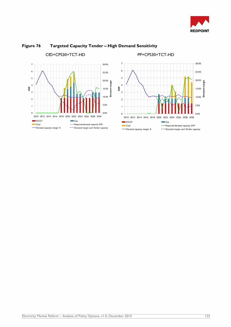
Electricity Market Reform – Analysis of Policy Options, v1.0, December 2010 122
Figure 76 Targeted Capacity Tender – High Demand Sensitivity
CfD+CPS30+TCT-HD PP+CPS30+TCT-HD
0.0%
5.0%
10.0%
15.0%
20.0%
25.0%
30.0%
2010 2012 2014 2016 2018 2020 2022 2024 2026 2028 2030
0
1
2
3
4
5
6
7
De
rate
d m
arg
in
GW
OCGT Gas
Coal Required derated capacity GW
Derated capacity margin % Derated margin excl. Tender capacity
0.0%
5.0%
10.0%
15.0%
20.0%
25.0%
30.0%
2010 2012 2014 2016 2018 2020 2022 2024 2026 2028 2030
0
1
2
3
4
5
6
7
De
rate
d m
arg
in
GW
OCGT Gas
Coal Required derated capacity GW
Derated capacity margin % Derated margin excl. Tender capacity

Electricity Market Reform – Analysis of Policy Options, v1.0, December 2010 123
Cost benefit analysis
Table 22 shows the cost benefit analysis for the combination packages under Central Demand assumptions
and the High Demand sensitivity relative to the Baseline under corresponding demand assumptions.
Table 22 Cost benefit analysis – High Demand sensitivity
Net welfare relative to Baseline over the period 2010-2030 appears higher for the combination packages
under the High Demand sensitivity. For example, a net welfare loss of around £4.6bn relative to the
Baseline under Central Demand assumptions becomes a net welfare gain of around £6.6bn under the High
Demand assumptions for the Contracts for Difference package. This increase in net welfare reflects the
fact that under the Baseline, the High Demand sensitivity results in greater use of less efficient existing fossil
plant which pushes up costs, and hence the savings from low-carbon investment are greater.
Under the High Demand sensitivity consumer surplus is significantly lower than the Baseline, and producers
are correspondingly better off, through a combination of the impacts on price of Carbon Price Support, and
in the case of the Contracts for Difference package, low underlying de-rated capacity margins. (As we
describe in Section 5.3, we have assumed that the Targeted Capacity Tender would be designed in such a
way as to leave wholesale prices unaffected, but in practice the impact on consumers will depend critically
on how the tendered capacity is utilised and priced into the market.)
Change in welfare
NPV 2010-2030,
(£m 2009 real)
Premium
Payments +
Carbon Price
Support (£30/t) +
Targeted
Capacity Tender
Contracts for
Difference +
Carbon Price
Support (£30/t) +
Targeted
Capacity Tender
Premium
Payments +
Carbon Price
Support (£30/t) +
Targeted
Capacity Tender
- High Demand
Contracts for
Difference +
Carbon Price
Support (£30/t) +
Targeted
Capacity Tender
- High Demand
Carbon costs 8,636 11,516 10,519 12,879
Generation costs 3,305 7,655 2,993 8,135
Capital costs -15,260 -23,973 -13,465 -14,476
Unserved energy 194 198 122 121
Demand side response -8 -18 -19 -45
Change in Net Welfare -3,132 -4,622 150 6,615
Wholesale price -14,727 -16,152 -24,232 -31,154
Low carbon payments 1,334 7,413 3,441 557
Capacity payments -1,176 -1,169 -1,104 -1,554
Unserved energy 194 198 122 121
Demand side response -8 -18 -19 -45
Change in Consumer Surplus -14,384 -9,728 -21,793 -32,074
Wholesale price 14,727 16,152 24,232 31,154
Low carbon support -1,368 -7,374 -3,405 -580
Capacity payments 1,176 1,169 1,104 1,554
Producer costs -14,207 -14,737 -11,100 -4,010
Change in Producer Surplus 329 -4,790 10,832 28,118
Net Welfare
Distributional analysis
Consumer
Surplus
Producer Surplus

Electricity Market Reform – Analysis of Policy Options, v1.0, December 2010 124
C Baseline assumptions
In this Appendix we outline our Baseline assumptions in more detail.
Fuel and carbon prices
Fuel price assumptions are based on DECC‟s Updated Energy Projections (UEP) June 2010 Central price
case. EU Allowance (EUA) carbon price assumptions are taken from DECC‟s Central assumptions.
Figure 77 Fuel and carbon prices assumptions
Demand
Growth in baseload demand is subject to mild cyclical variation, as may be seen in Figure 78. Total demand
falls in 2011, then grows strongly up to 2015, stalling in 2016 and 2017 and then growing strongly again
between 2018 and 2024. After 2024, baseload demand grows at a more modest pace. The relationship
between baseload and peak demand is based on historic analysis. The same cyclical pattern as that seen in
baseload demand growth may also be seen in peak demand growth.
Figure 78 Total and peak demand assumptions
0
20
40
60
80
100
120
2010 2012 2014 2016 2018 2020 2022 2024 2026 2028 2030
Coal price ($/t)
Gas price (p/th)
Carbon price (£/t)
40
50
60
70
80
90
100
200
250
300
350
400
450
500
2010 2012 2014 2016 2018 2020 2022 2024 2026 2028 2030
Peak
dem
and (
GW
)
Tota
l dem
and (
TW
h)
Total demand (TWh) Peak demand (GW)

Electricity Market Reform – Analysis of Policy Options, v1.0, December 2010 125
Capital costs
Capital cost assumptions for new build generation have been taken from the Mott MacDonald UK
Electricity Generation Costs Update report, June 201080.
Table 23 Capital cost assumptions
Capex, real 2010, £/kW FOAK NOAK
FOAK/NOAK
switch
Gas - CCGT 823 731 2010
Gas - CCGT with CCS 1,396 1,111 2010
Coal - IGCC with CCS 3,244 2,487 2010
Coal - ASC with FGD and CCS 3,128 2,479 2010
Nuclear - PWR 3,812 2,966 2010
Wind - Onshore 1,731 1,547 2010
Wind - Offshore 3,110 2,840 2010
Wind - Offshore R3 3,625 3,087 2018
Small biomass power only 2,820 2,540 2015
Large biomass power only 2,230 1,950 2020
Large biomass CHP 4,160 3,730 2020
Wave 3,559 3,559 2010
Tidal Stream 3,812 3,812 2010
Hydro 2,070 1,954 2010
Energy from Waste 6,150 5,120 2010
AD on wastes 4,170 3,900 2010
OCGT 474 438 2010
Note: For wave and tidal stream generation the capex figures given in Table 1 above are average values for years 2010 to 2034 inclusive. For
the remaining technologies the 2010 figures are given before any learning has taken place.
80
Downloaded from http://www.decc.gov.uk/assets/decc/statistics/projections/71-uk-electricity-generation-costs-update-.pdf and adjusted for
DECC exchange rate assumptions where appropriate.

Electricity Market Reform – Analysis of Policy Options, v1.0, December 2010 126
Learning
Table 24 Construction cost scalars
2010 2020 2030
Gas – CCGT 1.00 0.89 0.88
Gas - CCGT with CCS 1.00 0.90 0.89
Coal - IGCC with CCS 1.00 0.88 0.84
Coal - ASC with FGD and CCS 1.00 0.85 0.84
Nuclear – PWR 1.00 0.93 0.91
Wind – Onshore 1.00 0.90 0.89
Wind – Offshore 1.00 0.90 0.89
Wind - Offshore R3 1.00 0.90 0.89
Small biomass power only 1.00 0.88 0.86
Large biomass power only 1.00 0.95 0.87
Large biomass CHP 1.00 0.93 0.89
Wave 1.79 0.90 0.48
Tidal Stream 2.94 0.72 0.46
Hydro 1.00 1.00 1.00
Energy from Waste 1.00 1.00 1.00
AD on wastes 1.00 1.00 1.00
OCGT 1.00 1.00 1.00
Renewable Obligation
Table 25 RO banding assumptions – Baseline
2010 -2012 2013 -2016 2017 -2021 2022+
Co-firing (regular) 0.50 0.50 0.50 0.00
Co-firing (energy crops) 1.00 1.00 1.00 0.00
Wind – Onshore 1.00 1.30 0.75 0.25
Wind – Offshore 2.00 2.35 1.75 1.00
Small biomass power only 1.50 1.50 1.00 0.25
Large biomass power only 1.50 1.50 1.00 0.25
Large biomass CHP 2.00 2.00 1.00 0.25
Wave 2.00 4.00 4.00 2.00
Tidal Stream 2.00 4.00 4.00 2.00
Hydro 1.00 1.00 1.00 0.25
Energy from Waste 1.00 1.00 1.00 0.25
AD on wastes 2.00 2.00 2.00 0.50

Electricity Market Reform – Analysis of Policy Options, v1.0, December 2010 127
Planning and construction
Table 26 Plant build characteristics
Type Economic life
(years) Construction
(years)
Planning
(years)
Gas – CCGT 20 3 2
Gas - CCGT with CCS 25 4 2
Coal - IGCC with CCS 25 4 4
Coal - ASC with FGD and CCS 25 5 4
Nuclear – PWR 30 5 4
Wind – Onshore 20 2 5
Wind – Offshore 20 2 5
Wind - Offshore R3 20 2 5
Small biomass power only 20 2 2
Large biomass power only 20 4 2
Large biomass CHP 20 3 3
Wave 20 2 4
Tidal Stream 20 3 4
Hydro 20 5 5
Energy from Waste 20 3 3
AD on wastes 20 1 2
OCGT 20 2 2
Nuclear lifetime extensions
Table 27 Nuclear capacity, retirements and availability
Plant Capacity
(MW) Closure date Annual
availability
Dungeness B 1,110 2018 70%
Hartlepool 1,210 2019 70%
Heysham 1 1,150 2019 70%
Heysham 2 1,250 2028 70%
Hinkley Point 820 2016 70%
Torness 1,250 2028 70%
Hunterston 820 2016 70%
Sizewell B 1,190 2045 87%
Oldbury 434 2010 75%
Wylfa 980 2010 75%
Source: Nuclear Industry Association

Electricity Market Reform – Analysis of Policy Options, v1.0, December 2010 128
Capacity credits
Table 28 Capacity credits by technology
2010 2015 2020 2025 2030
Gas 90.0% 90.0% 90.0% 90.0% 90.0%
Coal 90.0% 90.0% 90.0% 90.0% 90.0%
CCS 90.0% 90.0% 90.0% 90.0% 90.0%
Nuclear (existing) 70.0% 70.0% 70.0% 70.0% 70.0%
Nuclear (new) 90.0% 90.0% 90.0% 90.0% 90.0%
Hydro 70.0% 70.0% 70.0% 70.0% 70.0%
Pumped storage 100.0% 100.0% 100.0% 100.0% 100.0%
Wind 27.5% 20.7% 17.5% 16.2% 16.2%
Marine 30.0% 30.0% 30.0% 30.0% 30.0%
Biomass 92.0% 92.0% 92.0% 92.0% 92.0%
Other renewables 30.0% 30.0% 30.0% 30.0% 30.0%
Tidal Range 12.8% 12.8% 12.8% 12.8% 12.8%
non ROC waste 40.0% 40.0% 40.0% 40.0% 40.0%
Oil 95.0% 95.0% 95.0% 95.0% 95.0%
GT 90.0% 90.0% 90.0% 90.0% 90.0%
Interconnector 95.0% 95.0% 95.0% 95.0% 95.0%

Electricity Market Reform – Analysis of Policy Options, v1.0, December 2010 129
D Estimating hurdle rates
Overview
A key hypothesis behind the analysis is that to the extent that EMR policy options reduce the risk for
different types of investment, the hurdle rate (and hence cost of capital) should reduce. Our assumptions
are informed by simulating the earnings risk over the lifetime of a project as described below.
Assumptions on hurdle rates are derived by estimating the impact of technology and market risk on the
cost of equity and project gearing levels, using benchmarks from recent projects where possible. We
assume that the hurdle rate for an investment is a function of both technology and development risk, which
is independent of the electricity market arrangements, and market risk, which is directly related to
electricity market arrangements.
The relative riskiness of the investment may affect the cost of equity, cost of debt and the gearing of the
project which in turn affects the overall hurdle rate.
For simplicity in the modelling, we vary the cost of equity to reflect differences in technology and
development risks for projects of different maturity, and vary the amount of gearing possible in the project
to reflect differences in market risk.
Our starting assumptions for the cost of capital for vertically integrated utilities and independent
developers are shown in Table 29 below. Note that these are long-run assumptions held constant
throughout the modelling time horizon.
The hurdle rates are calculated from these starting assumptions by varying the cost of equity and level of
gearing for individual projects.
Table 29 Assumptions for cost of capital
VIU Independent
Long-term risk
free rate 4%
Equity
premium 4% 4%
Debt premium 1.5% 3.0%
Typical equity
beta 0.71 1.75
Typical gearing 40% 70%
Corporation
tax rate 24%
Typical WACC 6% 7%

Electricity Market Reform – Analysis of Policy Options, v1.0, December 2010 130
Technology and development risk
We model the technology and development risk by varying the cost of equity which involves scaling the
equity premium by an „investment beta‟ dependent on the maturity of each technology as follows:
Cost of equity = risk free rate + market premium * equity beta * investment beta
For mature technologies we assume an investment beta of 2, for established technologies an investment
beta of 3 and for emerging technologies an investment beta of 4.
Table 30 below shows our assumptions for the maturity of different technologies by year.
Table 30 Technology maturity assumptions
Technology 2010 2015 2020 2025 2030
CCGT Mature Mature Mature Mature Mature
Gas - CCGT with CCS Emerging Emerging Emerging Emerging Established
Coal - IGCC with CCS Emerging Emerging Emerging Emerging Established
Coal - ASC with FGD & CCS Emerging Emerging Emerging Emerging Established
Nuclear Emerging Emerging Established Established Mature
Wind - Onshore (High) Mature Mature Mature Mature Mature
Wind - Onshore (Medium) Mature Mature Mature Mature Mature
Wind - Onshore (Low) Mature Mature Mature Mature Mature
Wind - Offshore Established Established Mature Mature Mature
Wind - Offshore R3 Emerging Emerging Established Established Mature
Small biomass power only Emerging Emerging Established Established Mature
Large biomass power only Emerging Emerging Established Established Mature
Large biomass CHP Emerging Emerging Established Established Mature
Wave Emerging Emerging Emerging Emerging Established
Tidal Stream Emerging Emerging Emerging Emerging Established
Hydro Mature Mature Mature Mature Mature
Energy from Waste Established Established Established Mature Mature
AD on wastes Emerging Emerging Emerging Established Mature
OCGT Mature Mature Mature Mature Mature
These assumptions yield a range in hurdle rates (post tax nominal) from around 8% for mature
technologies to around 12% for emerging technologies for VIUs under current market arrangements. The
equivalent range for independent developers is 9-13%.
Market and policy risk
For the purposes of the analysis, we assume that where the impact of a different policy is to reduce
expected earnings risk, the level of debt in the project can be correspondingly increased.
To do this, we first simulate overall earnings risk over the lifetime of the project, taking account of all key
drivers: fuel costs, carbon costs, capital costs, construction times, operating costs, availability, electricity
prices, support levels, load factor, and balancing risk. Using this we can then assess the incremental impact

Electricity Market Reform – Analysis of Policy Options, v1.0, December 2010 131
of policy options. Where policies reduce earnings risk, for example by reducing revenue uncertainty, it is
assumed a greater proportion of the project could be financed with lower cost capital.
We compare the earnings at risk over the lifetime of an investment under each policy option to the
Baseline. The simulation of earnings risk is illustrated in Figure 79 below. The „earnings-at-risk‟ is
calculated as the difference between the mean earnings expectation and a downside case represented by
the 95% percentile. This is then expressed as a percentage of the mean. In broad terms a reduction in
earnings-at-risk corresponds to a similar increase in the proportion of “safe” earnings, and hence enables an
equivalent increase in the proportion of potential debt financing. For example, if the impact of a policy
option to is to reduce the earnings at risk by 10 percentage points we assume that it is possible to increase
gearing in the project likewise by 10 percentage points. For vertically integrated utilities, this may not
literally be the case since projects may be more or less balance sheet financed. However, the ability to
raise debt to fund investment across the business will depend on the market‟s perceived riskiness of a
company‟s investments and hence a similar principle can be considered.
Figure 79 Simulated earnings risk
We assume that the cost of debt increases with the level of gearing, particularly for less mature
technologies, but is cheaper than the cost equity.
We also assume that there is a maximum level of gearing possible in projects, regardless of market risk,
associated with technology maturity as follows:
Mature: 90%
Established: 80%
Emerging: 75%
Levelised earnings
Pro
bab
ilit
y
Mean95%
“Earnings
at risk”
Increased gearing
possibleReduction
in EaR

Electricity Market Reform – Analysis of Policy Options, v1.0, December 2010 132
E Modelling approach
In this Appendix, we briefly outline our modelling approach, describing at a high level the modelling
framework we have used, and explaining the capacity credit concept in more detail.
Modelling framework
Figure 80 Modelling framework
At the heart of the modelling framework deployed for this study lies an investment decisions simulator.
This computes the risk-adjusted LRMCs of all generation technologies by player type. Where these are
less than expected revenues (given assumed load factors and future price expectations), players move new
plant first to a planning stage, and subsequently, if still economic, to a committed development phase. On
an annual basis, outturn results for demand, prices, generation output and carbon emissions are computed.
These in turn feed back to expected prices for the following year‟s iteration.
The LRMCs used in the build decision algorithm are risk-adjusted in the risk adjustment calculator by
computing a distribution of earnings for each investment under the full range of uncertainties in revenues
and project costs. The volatility model analyses the market at an hourly level for each year by simulating
demand, spot fuel prices, forced outages and renewables output. It produces annual price duration curves
and estimates of price volatility and volumes of short-term demand side response and expected energy
unserved81. It is used to calibrate the expected price and renewables „capacity credit‟ functions within the
investment decisions simulator.
81
A full stochastic simulation is run using the volatility model in order to derive the unserved energy numbers under the Baseline. For all other
packages, unserved energy numbers are derived using an estimated relationship between the de-rated peak capacity margin and unserved energy, that relationship itself being derived from a volatility model simulation.
Scenario
assumptions
Annual iterations Modelling
period results
LRMCs
Risk adjusted
required price
Expected
prices
Build
decisions
Demand
Prices
Costs
CO2 emissions
Investment decisions Outturn results
•Installed capacity
•Achieved renewables
generation
•Subsidy cost
•CBA
•Fuel prices
•Supply curves
•Max build rates
•Capital costs
•Financing costs
•Operating costs
Volatility model
•Capacity factors
•Price shape
•Unserved energy
Risk adjustment
calculator
• Risk premia
• by investor
• by technology
Policy option
Electricity Market Reform – Analysis of Policy Options, v1.0, December 2010 133
Capacity credit
The capacity credit is the statistical contribution of a particular class of generation to security of supply.
The capacity credit for intermittent renewables is often expressed as the amount of conventional thermal
generation (taking into account its likelihood of availability) that intermittent generation could effectively
“replace”, without any reduction in security of supply. It is therefore a useful concept when incorporating
different types of generation capacity into a calculation of de-rated capacity margin on an equivalent basis.
Measuring the capacity credit of intermittent generation (wind, wave, tidal) is complex since it is a function
of the amount, type and geographical distribution of generation plant on the system. The capacity credit
for total installed intermittent capacity will generally be lower than the sum of individual plant capacity
factors. In particular, the average capacity credit for a given technology will be affected by:
the total existing installed capacity of that technology on the system, and
the geographical distribution of different intermittent technologies and relationships between
output levels at different locations.
The first of these factors results from the fact that the output levels of individual units of intermittent
capacity of any single technology (such as wind) are generally correlated. As a result, while the first unit of
a technology deployed may have a capacity credit close to its capacity factor, the average capacity credit
declines as the installed capacity of that technology increases. Each extra unit of installed capacity yields a
diminishing marginal contribution to security of supply, because of the high likelihood that its output profile
(and especially its zero-output hours) will be correlated with those of the remainder of the installed
capacity. For the example of wind, the first MW on the system may have a marginal capacity credit of close
to 30%, whereas the 40,000th MW may have a marginal capacity credit below 5%. Thus the difference
between each additional unit‟s capacity factor (constant) and its capacity credit (diminishing) increases with
penetration, and the amount of conventional capacity required to back up each additional MWh of output
increases as more renewables capacity is built.

Electricity Market Reform – Analysis of Policy Options, v1.0, December 2010 134
F Results metrics
In this Appendix we describe the key metrics summarising the modelling results that are presented in the
report.
Decarbonisation
The extent of decarbonisation of the GB electricity sector is measured in terms of the carbon dioxide
emissions intensity of the GB electricity generation system as a whole. The unit of measure for emissions
intensity is g/kWh. Our modelling only measures the direct emissions from fossil fuel generation and does
not take into account emissions relating to the entire life-cycle of generation technologies or fuel
production.
Generation mix
For every year between 2010 and 2030, the model outputs the resulting generation mix in every model
run, measured in GW of capacity. This is based on the existing generation capacity mix at the start of that
year plus any capacity that is built in that year and minus any capacity retired in the model. Total capacity is
summarised into categories that may be seen in Figure 5.
The generation mix profile, together with capacity credits and assumptions on peak demand, feeds into
security of supply analysis as it is used to derive the de-rated peak capacity margin.
Security of supply
The key indicator we use to assess security of supply between packages is the de-rated peak capacity
margin. This is a measure of expected peak availability compared to peak demand. This takes into account
the capacity credit, which measures the percentage of maximum potential output that statistically can be
shown to contribute to security of supply. For conventional plant this will cover forced outages, and for
intermittent (wind and wave) and variable-output (tidal) renewables it will in addition account for expected
output based on probabilistic analysis of resource levels. The methodology for modelling capacity credit of
intermittent and variable-output renewables is described in Appendix E.
Resource costs
Resource costs, which are calculated in the model as part of the cost benefit analysis, consist of the
following elements.
• Carbon costs represent the welfare loss associated with carbon dioxide emissions. They are
calculated on the basis of the EUA price in the year in which emissions occur.
• Generation costs include all variable and fixed costs of the GB generation system, including fuel
costs, but excluding carbon costs. They represent running costs of generation. These are
calculated from DECC assumptions for new capacity built in the model and a mixture of DECC
and Redpoint assumptions for existing and committed generation capacity as of 2010 in the
model.
• Capital costs represent total debt and equity costs of new generation capacity built in the model.
They are based on assumptions on construction costs, debt and equity costs, leverage and gearing
levels.
Cost to consumers
This is a measure of the price of the energy component of electricity for a typical consumer, normally
quoted in £/MWh. It is the sum of wholesale electricity costs, the cost of low-carbon support, and capacity

Electricity Market Reform – Analysis of Policy Options, v1.0, December 2010 135
payments (if applicable). It excludes non-energy items such as transmission and distribution charges,
supplier margin and VAT.
Wholesale electricity prices are clearly a key driver of the consumer cost. While the level of wholesale
price is dominated by the commodity price levels, there are significant differences between packages. This
is a result of the different resulting capacity build profiles, which in turn change both the supply curve
through the year, and hence the system marginal price, and the year-to-year system capacity margin, with a
resulting impact on price „uplift‟.
Economic Rent
Economic rent is the additional earnings achieved by a generator above the level required to cover
operating costs, debt costs, and to earn a reasonable return on investment. Under the RO as it stands,
rents for renewables generators are strongly influenced by the level of wholesale prices, as the RO
effectively provides a premium payment on top of wholesale electricity revenues. However, even under
packages we have modelled with fixed payments, there will always be a spread of rents both because of the
variation of costs of technologies within a given „band‟ or tariff category, and differences in the costs of
financing for different player types.
Rent is presented under three different categories through this report. This is measured in £m, and is the
total rent achieved by a particular plant type in a given year:
- Rent for existing renewables
- Rent for new renewables
It should be noted that for future plant that are developed endogenously within the model, the reported
rent is internally consistent, as there is a precise (modelled) definition of each of the components. This
differs from existing plant, for which the actual costs are not precisely known to us. As such, the absolute
level of reported rent in the early part of the modelling horizon (where existing plant dominate the mix)
should be treated with caution. This does not detract from the messages to be drawn from the relative
differences in rent between packages.
Electricity Market Reform – Analysis of Policy Options, v1.0, December 2010 136
G Cost benefit analysis
In this Appendix we describe the cost benefit analysis approach used in the project, and present additional
CBA results for sensitivities and combination packages.
Cost benefit analysis: approach
The costs and benefits of each of the options are measured against the Baseline as the counterfactual. They
are calculated annually and as a net present value (NPV) for the period 2010-2030 using the Green Book
real discount rate of 3.5% and presented in real 2009 terms. It is important to note that the NPV analysis
does not capture the costs and benefits of the options after 2030.
A key point that must be understood in the evaluation of any policy in relation to low-carbon investment is
that low-carbon generation is generally more expensive than conventional thermal plant under the Baseline
assumptions. As there is no explicit penalty for missing the targets. or evaluation of the unquantified
impacts of diversifying the generation portfolio, options that meet the decarbonisation targets will typically
result in lower net welfare compared to options that fall short. This difference can be considered as the
cost to society of meeting the targets, and different options can be compared on this basis.
Each component of the cost benefit analysis is described below.
Carbon costs. The change in value of carbon dioxide emissions as measured using the cost
of EU Allowances (EUAs). A positive number represents a decrease in carbon dioxide
emissions (i.e., a saving in EU ETS allowance costs to the GB power sector).
Generation Costs. The change in the costs of generating electricity, including changes in fuel
costs, variable and fixed operating costs and system balancing costs. It excludes changes in the
costs of carbon which are captured above, and capital costs which are captured below. A
negative number represents an increase in generation costs relative to the counterfactual.
Capital costs. The change in capital expenditure in new plant. A negative number
represents an increase in capital costs.
Unserved energy. The change in the cost of expected energy unserved, which is valued at
an average £10,000/MWh. A negative number implies an increase in the cost of unserved
energy and a deterioration in security of supply.
Demand side response. The change in the use of short-term demand side response. A
reduction in demand in response to high prices represents a loss of consumer welfare82.
Net welfare. The change in welfare to society as a whole which is equivalent to the sum of
the change in carbon costs, generation costs, capital costs, unserved energy and demand side
response. A negative number represents a loss in net welfare to the economy.
Consumer surplus. The change in welfare to consumers, which is a combination of the
change in wholesale electricity costs, change in the low-carbon payments, and the change in
capacity payments (where these apply). A negative number represents a reduction in
consumer surplus or an increase in the costs to consumers.
Producer surplus. The change in the profitability of the generation sector measured as the
change in the difference between revenues (electricity sales, low-carbon support and capacity
payments) and producer costs. A positive number represents an increase in the producer
surplus.
82
Note we do not consider the long-term price elasticity of demand in the cost benefit analysis.

Electricity Market Reform – Analysis of Policy Options, v1.0, December 2010 137
Cost benefit analysis: Low Gas
Table 31 shows the cost benefit analysis under the Low Gas sensitivities, relative to the Baseline-Low Gas.
Net welfare appears much lower under Fixed Payments and Contracts for Difference than the other
options since these deliver more low-carbon investment which is relatively more expensive than the
alternative (ie, gas) generation under this sensitivity. In Carbon Price Support (£50/t), Strong EPS and
Premium Payments, investment in low-carbon generation is reduced and so the net welfare loss is smaller,
although the decarbonisation and renewable energy targets are not met.
Consumers are worse off under all the policy options since electricity prices are considerably higher than
the Baseline-Low Gas due to some occasions of very low de-rated capacity margins.
Table 31 Cost benefit analysis – Low Gas Sensitivity
Cost benefit analysis: High Gas
Table 32 shows the cost benefit analysis for the High Gas sensitivity. Net welfare is positive under Fixed
Payments and Contracts for Difference relative to the Baseline as savings in carbon costs and generation
costs relative to the Baseline outweigh the additional capital costs of new generation capacity. Under the
options where low-carbon generators are still exposed to wholesale price – Carbon Price Support (£50/t),
Strong EPS and Premium Payments – net welfare decreases since they „over-deliver‟ low-carbon
investment.
Consumers are significantly better off under the High Gas price sensitivity under Fixed Payments and
Contracts for Difference. From approximately 2020 onwards, the price paid to low-carbon generators is
on average lower than the electricity price under Fixed Payments and Contracts for Difference with a High
Gas price.
Change in welfare
NPV 2010-2030,
(£m 2009 real)
Carbon Price
Support (£50/t) -
Low Gas
EPS - Low Gas
Premium
Payments - Low
Gas
Fixed Payments -
Low GasCfDs - Low Gas
Carbon costs 5,735 2,965 2,742 11,283 11,174
Generation costs -516 -6,931 115 4,441 4,845
Capital costs -7,287 -1,656 -11,071 -35,211 -35,600
Unserved energy -54 -44 -717 -409 -421
Demand side response -4 -2 -55 -21 -23
Change in Net Welfare -2,126 -5,668 -8,985 -19,916 -20,025
Wholesale price -37,897 -46,328 -25,559 -8,842 -9,670
Low carbon payments 5,541 5,747 -5,313 -27,926 -24,440
Capacity payments 0 0 0 0 0
Unserved energy -54 -44 -717 -409 -421
Demand side response -4 -2 -55 -21 -23
Change in Consumer Surplus -32,414 -40,626 -31,643 -37,198 -34,554
Wholesale price 37,897 46,328 25,559 8,842 9,670
Low carbon support -5,442 -5,679 5,127 28,261 24,767
Capacity payments 0 0 0 0 0
Producer costs -20,988 -5,622 -8,214 -19,487 -19,581
Change in Producer Surplus 11,467 35,027 22,472 17,616 14,856
Net Welfare
Distributional analysis
Consumer
Surplus
Producer Surplus

Electricity Market Reform – Analysis of Policy Options, v1.0, December 2010 138
Table 32 Cost benefit analysis – High Gas Sensitivity
Cost benefit analysis: Low Carbon
Table 33 shows the cost benefit analysis for the Low Carbon sensitivity. All options show negative net
welfare under the Low Carbon sensitivity since they deliver more low-carbon investment relative to the
Baseline, which is more expensive than new build under the Baseline, but the value placed on the resulting
decarbonisation is lower as this is based on the lower EUA prices.
Consumers are worse off as a result, particularly under Carbon Price Support (£50/t), where a very large
gap between the carbon price support level and the EUA price introduces distortion to economic dispatch
on top of distortion to investment incentives.
Change in welfare
NPV 2010-2030,
(£m 2009 real)
Carbon Price
Support (£50/t) -
High Gas
EPS - High Gas
Premium
Payments - High
Gas
Fixed Payments -
High GasCfDs - High Gas
Carbon costs 14,610 15,595 10,469 7,183 6,649
Generation costs -5,663 -19,155 6,562 5,961 6,181
Capital costs -18,840 -14,257 -24,111 -12,142 -11,002
Unserved energy 266 277 -178 -30 -104
Demand side response 31 32 -15 -7 -14
Change in Net Welfare -9,597 -17,508 -7,272 964 1,711
Wholesale price -17,970 -19,128 20,568 11,161 6,587
Low carbon payments 10,034 11,683 -13,104 10,778 17,285
Capacity payments 0 0 0 0 0
Unserved energy 266 277 -178 -30 -104
Demand side response 31 32 -15 -7 -14
Change in Consumer Surplus -7,639 -7,137 7,272 21,902 23,754
Wholesale price 17,970 19,128 -20,568 -11,161 -6,587
Low carbon support -10,157 -11,587 13,144 -10,949 -17,535
Capacity payments 0 0 0 0 0
Producer costs -36,034 -17,817 -7,079 1,001 1,828
Change in Producer Surplus -28,220 -10,275 -14,504 -21,108 -22,293
Net Welfare
Distributional analysis
Consumer
Surplus
Producer Surplus

Electricity Market Reform – Analysis of Policy Options, v1.0, December 2010 139
Table 33 Cost benefit analysis – Low Carbon Sensitivity
Cost benefit analysis: Capacity Payments for All
Table 34 shows the cost benefit analysis under Options to promote decarbonisation with Capacity
Payments for All relative to the Baseline. Introducing Capacity Payments for All together with support for
low-carbon generation generally leads to a reduction in net welfare relative to the Baseline since the
additional resource costs associated with having more capacity on the system are greater than the savings
in expected energy unserved, and carbon emission savings are valued at the EUA price, which remains low
until after 2020.
The distributional effects of Capacity Payments for All and support for low-carbon generation are much
greater than the overall net welfare impact. Consumers appear worse off relative to the Baseline for the
reasons described above. Correspondingly, producers are significantly better off, particularly under
Carbon Price Support (£50/t) and Strong EPS. In the case of these two packages, consumers lose out due
to significantly higher wholesale electricity prices than under the Baseline. This is also the case for these
policy packages without capacity payments.
Change in welfare
NPV 2010-2030,
(£m 2009 real)
Carbon Price
Support (£50/t) -
Low Carbon
EPS - Low
Carbon
Premium
Payments - Low
Carbon
Fixed Payments -
Low Carbon
CfDs - Low
Carbon
Carbon costs 11,575 10,112 3,801 6,245 5,837
Generation costs -9,860 -8,811 2,265 9,196 8,704
Capital costs -20,685 -22,387 -18,541 -28,084 -27,826
Unserved energy 152 122 -316 -57 -110
Demand side response 21 17 -26 -5 -12
Change in Net Welfare -18,796 -20,945 -12,817 -12,704 -13,408
Wholesale price -61,953 -35,272 -6,419 12,199 7,215
Low carbon payments 6,191 7,762 -10,667 -19,454 -13,997
Capacity payments 0 0 0 0 0
Unserved energy 152 122 -316 -57 -110
Demand side response 21 17 -26 -5 -12
Change in Consumer Surplus -55,589 -27,370 -17,428 -7,316 -6,904
Wholesale price 61,953 35,272 6,419 -12,199 -7,215
Low carbon support -6,187 -7,483 10,635 19,429 13,964
Capacity payments 0 0 0 0 0
Producer costs -54,575 -21,085 -12,475 -12,642 -13,285
Change in Producer Surplus 1,191 6,704 4,579 -5,412 -6,536
Net Welfare
Distributional analysis
Consumer
Surplus
Producer Surplus

Electricity Market Reform – Analysis of Policy Options, v1.0, December 2010 140
Table 34 Cost benefit analysis – Capacity Payments for All
Cost benefit analysis: Combination packages
Table 35 shows the cost benefit analysis under Combination packages relative to the Baseline. The
Combination packages lead to lower net welfare relative to Baseline. This is the due to the distortion of
dispatch economics towards more expensive fuels as a result of Carbon Price Support and the fact that the
cost of the tendered capacity is greater than the assumed savings in the cost of unserved energy.
Consumer surplus falls under the combination packages, with the dominant factor being the increase in
wholesale prices associated with Carbon Price Support. This is offset to some extent by the reduced need
for direct low-carbon support. There are additional costs for consumers associated with the Targeted
Capacity Tender, but these are relatively small.
Change in welfare
NPV 2010-2030,
(£m 2009 real)
Carbon Price
Support (£50/t)
& Capacity
Payments For
All
Strong
Emissions
Performance
Standard +
Capacity
Payments For
All
Premium
Payments +
Capacity
Payments For
All
Fixed Payments
+ Capacity
Payments For
All
Contracts for
Difference +
Capacity
Payments For All
Carbon costs 13,930 10,427 5,954 9,825 11,520
Generation costs -6,852 -7,895 1,481 9,205 12,796
Capital costs -10,093 -6,239 -18,377 -23,920 -28,551
Unserved energy 236 196 232 228 161
Demand side response 46 36 44 43 26
Change in Net Welfare -2,733 -3,474 -10,666 -4,620 -4,049
Wholesale price -21,176 -26,688 24,733 30,915 33,809
Low carbon payments 2,127 5,611 -16,836 -12,152 -7,113
Capacity payments -35,136 -35,120 -35,136 -29,196 -35,099
Unserved energy 236 196 232 228 161
Demand side response 46 36 44 43 26
Change in Consumer Surplus -53,903 -55,964 -26,963 -10,162 -8,216
Wholesale price 21,176 26,688 -24,733 -30,915 -33,809
Low carbon support -2,200 -5,591 16,873 12,179 7,083
Capacity payments 35,136 35,120 35,136 29,196 35,099
Producer costs -26,290 -3,707 -10,942 -4,890 -4,236
Change in Producer Surplus 27,822 52,510 16,334 5,569 4,137
Net Welfare
Distributional analysis
Consumer
Surplus
Producer Surplus
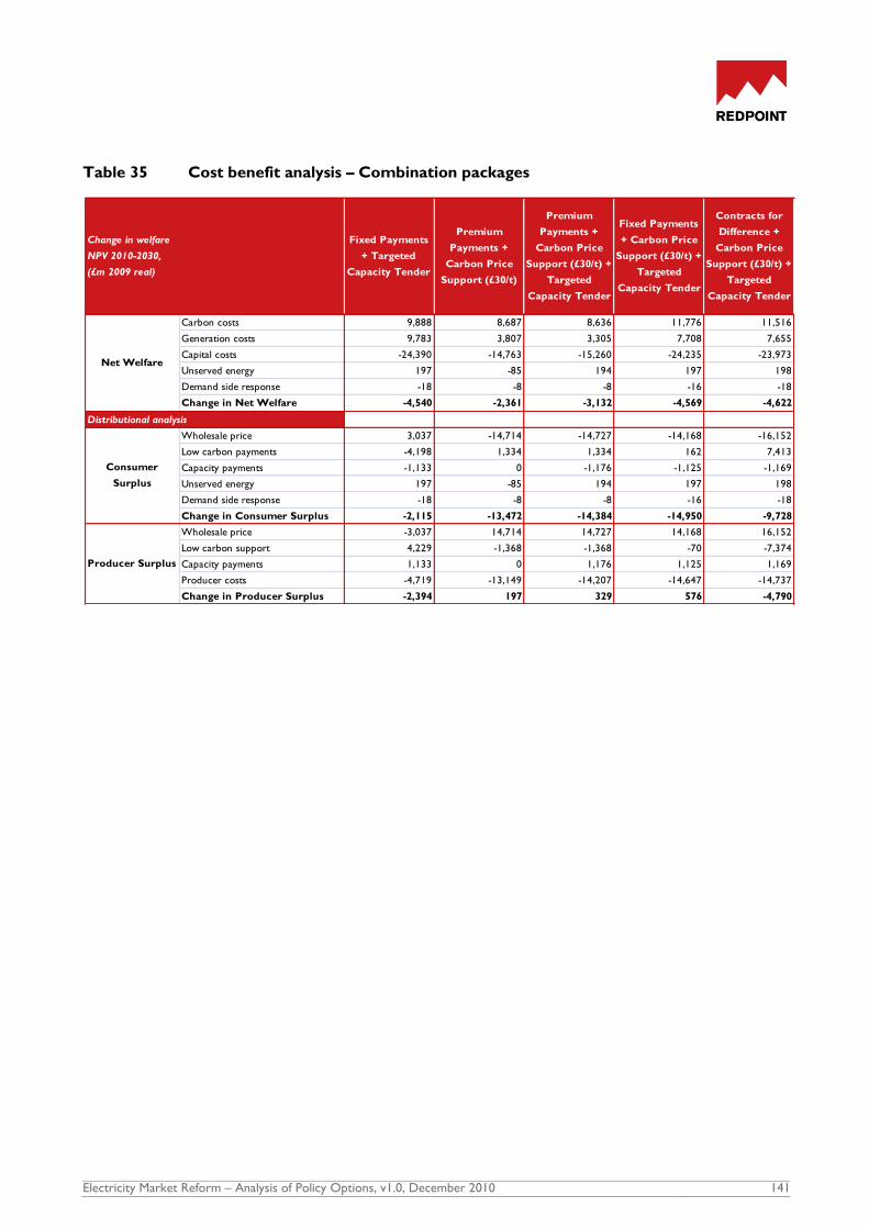
Electricity Market Reform – Analysis of Policy Options, v1.0, December 2010 141
Table 35 Cost benefit analysis – Combination packages
Change in welfare
NPV 2010-2030,
(£m 2009 real)
Fixed Payments
+ Targeted
Capacity Tender
Premium
Payments +
Carbon Price
Support (£30/t)
Premium
Payments +
Carbon Price
Support (£30/t) +
Targeted
Capacity Tender
Fixed Payments
+ Carbon Price
Support (£30/t) +
Targeted
Capacity Tender
Contracts for
Difference +
Carbon Price
Support (£30/t) +
Targeted
Capacity Tender
Carbon costs 9,888 8,687 8,636 11,776 11,516
Generation costs 9,783 3,807 3,305 7,708 7,655
Capital costs -24,390 -14,763 -15,260 -24,235 -23,973
Unserved energy 197 -85 194 197 198
Demand side response -18 -8 -8 -16 -18
Change in Net Welfare -4,540 -2,361 -3,132 -4,569 -4,622
Wholesale price 3,037 -14,714 -14,727 -14,168 -16,152
Low carbon payments -4,198 1,334 1,334 162 7,413
Capacity payments -1,133 0 -1,176 -1,125 -1,169
Unserved energy 197 -85 194 197 198
Demand side response -18 -8 -8 -16 -18
Change in Consumer Surplus -2,115 -13,472 -14,384 -14,950 -9,728
Wholesale price -3,037 14,714 14,727 14,168 16,152
Low carbon support 4,229 -1,368 -1,368 -70 -7,374
Capacity payments 1,133 0 1,176 1,125 1,169
Producer costs -4,719 -13,149 -14,207 -14,647 -14,737
Change in Producer Surplus -2,394 197 329 576 -4,790
Net Welfare
Distributional analysis
Consumer
Surplus
Producer Surplus