electrically synchronised gear shifting industrial ... document/5218_full... · dept. of industrial...

Indust

rial E

lectr

ical Engin

eering a

nd A

uto

mation

CODEN:LUTEDX/(TEIE-5218)/1-74/(2006)

Electrically synchronised gear shifting

Per Bandrup and Joakim Larsson

Dept. of Industrial Electrical Engineering and Automation Lund University

Abstract

Electrically synchronised gear shifting is a new way of solving the old gearbox problem

and a new way of building a light hybridised vehicle. A 10kW electrical machine, which

is used to synchronise the speed of the outgoing and incoming shafts during a gearshift,

replaces the function of the classic clutch in the gearbox. The clutch is kept, but only used

during start and when the vehicle is driven in pure electric mode. The gearbox is fitted

with a servo actuator, making a gear-shifting robot, to move the gear stick and to shift

gears automatically and very fast. The gear shifting sequence is as follows:

• First the torque is set to zero by setting all currents to zero

• Then the gearbox is put into neutral

• A speed controller is temporarily applied to the electrical machine to synchronise

the outgoing and incoming shafts of the gearbox

• The new gear is applied

• Finally the gear stick is returned to its home position and the torque is reapplied

The total time of torque loss is the time for putting the gearbox into neutral,

synchronising the speed and applying the new gear.

A sequential racing gearbox that is fitted with a 10kW permanent magnetised

synchronous machine and a servo actuator from SEW is used to test the concept of

electrically synchronised gear shifting. The gearbox is mounted in a rig fitted with

flywheels with the same inertia as the rotating masses of a real car. A computer with

dSpace and a tailor made DC-AC power converter is used to control the traction motor

and the gear-shifting robot.

2

The electrical machine is modelled using Matlab Simulink from which it is determined

that the electrical machine can be braked 15 % @ 1200 rpm, in 70 ms and accelerated in

120 ms using all of the available torque. Simulations with altered motor design is also

made and by decreasing the diameter from 300 mm to 180 mm and by making the motor

150 mm long instead of 70 mm the motor inertia is cut by a factor three. The acceleration

ability can be cut by almost the same factor but is still limited by the inertia of the

incoming shaft and gears in the gearbox.

The results from the laboratory experiments give a total torque loss time of 280ms of

which the speed synchronisation is 70ms during shift up and 120ms during shift down.

The rest of the time is for moving the servo arm and some communication lag.

By redesigning the electrical traction motor, replacing the servo and its controller to a

faster one and by building an optimised gearbox with the same relative gear ratio and

without the synchronisation rings it should be possible to cut the torque loss times to less

than 100ms.

3

Table of Contents Acknowledgements ..................................................................................................................................6 1 Introduction to electrically synchronised gear-shifting.....................................................7 2 Goal and limitations........................................................................................................................9 3 Modelling ..........................................................................................................................................10

3.1 Electric traction motor sizing...........................................................................................10 3.1.1 Inner rotor motor .......................................................................................................10

3.2 Modelling the permanent magnet synchronous machine.....................................13 3.3 Simulation results ................................................................................................................18 3.4 The gear shifting sequence ..............................................................................................21

4 The laboratory equipment..........................................................................................................22 4.1 Basic control of permanent magnetized synchronous machine.........................32 4.2 Implementation of a simple field-weakening controller........................................33 4.3 Control of the gear-shifting robot..................................................................................34 4.4 A short description of the computer program...........................................................36 4.5 The computer interface .....................................................................................................37

5 Results ...............................................................................................................................................38 5.1 Experimental results...........................................................................................................38 5.2 Early results ...........................................................................................................................38

5.2.1 Shifting up.....................................................................................................................39 5.2.2 Shifting down ...............................................................................................................40 5.2.3 Discussion .....................................................................................................................41

5.3 Improvements to the systems........................................................................................41 5.4 Further results ......................................................................................................................42

5.4.1 Shifting up.....................................................................................................................42 5.4.2 Shifting down ...............................................................................................................43 5.4.3 Discussion .....................................................................................................................44

5.5 Final results............................................................................................................................45 5.5.1 Shifting up.....................................................................................................................45 5.5.2 Shifting down ...............................................................................................................47 5.5.3 Discussion .....................................................................................................................48

6 Discussion ........................................................................................................................................49 7 Conclusions and recommendations ........................................................................................51

7.1 Optimised gearbox ..............................................................................................................51 7.1.1 Optimal PMSM..............................................................................................................51 7.1.2 System optimisation .................................................................................................52

8 References .......................................................................................................................................54 Appendix A ................................................................................................................................................56 Appendix B ................................................................................................................................................69

The Four-wire method...................................................................... Error! Bookmark not defined. Two-wire measurement ...................................................................................................................69 The four wire method .......................................................................................................................71

4

Measurement error and applications ..........................................................................................71 High resistance measurements ....................................................................................................72 Power line noise voltages................................................................................................................72

Appendix C ................................................................................................................................................74

5

Acknowledgements We would like to express our gratitude to Professor Mats Alaküla for invaluable help

with the simulations and the calculations. A special thanks to Roland Andersson, Lars

Hoffman, Tommy Lindholm and all other at SAAB Automobile for support and building

of the laboratory rig. Thanks to Stefan Blomgren and Daniel Karlsson at Binar

Electronics for support with the gear shifting robot. We would also like to thank PhD-

student Jonas Ottosson for most inspiring conversations and engineer Bengt Simonson for

help with the laboratory setup. Special thanks to PhD-student Tomas Bergh, and David

Dufke, technical doctor Per Karlsson and engineer Andreas Sörensen for help with the C-

code and the power electronics. Our deepest gratitude to research engineer Getachew

Darge for invaluable help with the laboratory setup. A special thanks to Limhamns

Industriservice AB for letting us borrow lathe and grinder. Thanks to Zivorad Zivkovic at

the division of solid mechanics LTH, Jan-Erik Nilsson at the division of combustion

engines LTH, Ingjald Andreasson at the division of heat transfer, and Thorsten Jacobsson

at the department of machine elements LTH for support with tools and machines. Finally

we would like to express our thanks to friends and family.

6

1 Introduction to electrically synchronised gear-shifting

With rising oil prices and environmental issues, the subject of efficiency and fuel

consumption is becoming more and more important. The system efficiency of

combustion engine based drive trains is subject to improvement. The alternative of

hybridisation is an interesting option that can be designed in many different ways. Every

part of such a system must be optimised. One of these parts is the gearbox, a part that has

looked almost the same for over 60 years. Throughout the history there have mainly been

two different gearboxes, the manual and the automatic. Several different complex

automatic or semi-automatic gearboxes have been presented as a way to change the

standard, however at an increased system cost. In hybrid vehicles the efficiency aspect is

the most critical when selecting a gearbox. The recent hybrid-vehicles on the market use

more complex and expensive transmissions.

The hybrid project reported here is focused on a new way of solving the gearbox-

problem. It uses the traditional manual gearbox but without the synchronisation-rings. In

order to maintain the system efficiency at highest possible level in hybrid vehicles it is

necessary to not let the driver decide when to shift gears, but instead let a computer

calculate the best working point at all time. The movement of the gear selector in this

laboratory setup uses a "shift robot". The system also holds a permanent magnet

synchronous machine (PMSM) mounted on the incoming axle of the gearbox to

implement a light hybridisation, see figure 1. This PMSM also works as the

synchronisation of the gearbox and replaces the synchronisation rings and the normal

clutch in the gearbox. The clutch is kept but is only used during take off and to give the

opportunity of pure electrical propulsion in cities and pollution sensitive areas. The

gearbox itself is intended to hold as many as up to seven or eight gears in order to lower

7

the gear-ratio difference between the gears in the gearbox. The idea is also to have the

same relative gear ratio between the gears by keeping the first and last gears as they are

and even out the gear ratio difference between different gears. This causes the gear

shifting to become smoother and the shifting-times to be shorter, something that is

required in order for the driver not to perceive the loss of torque during acceleration.

The advantages of this system are, most important, its simplicity compared to planetary-

based gearbox solutions and other systems on the market but also the compact size and

cheap design. Further, only one electrical machine, one clutch and one set of power

electronics is needed which makes the concept cheap compared to all other known

systems. The gearbox can be simplified, shortened and produced cheaper since the

synchronisation rings are no longer needed. By shortening the gearbox more space is left

for the electrical traction motor. Another benefit is that it still keeps the possibility to let

the driver do the gear shifting, something that is sought after by many buyers.

PMSM

DIFFERENTIAL

Figure 1 The gearbox topology

8

2 Goal and limitations The main goal of this project is to prove that the concept of electrically synchronised gear

shifting, as described in the introduction, is possible and what limitations and possibilities

that lays within the concept. The project also aimed to determine whether it was possible

to build a light, hybridised vehicle using this concept. The project were split into the

following sub-goals:

• Use a custom-built three-phase DC to AC converter to run a permanent

magnetized synchronous machine

• Set up the gear-shifting device in a laboratory system.

• Develop control methods and make experiments.

A rather moderate gear step with an rpm difference of 15% was chosen. This corresponds

to the rpm difference between step four and five in the gearbox used. The reason for this

is that within the concept lies the thought of having gear steps with the same relative gear

ratio in the gearbox. Since the synchronisation rings are no longer needed they can be

removed. This makes it possible to add more gears by keeping the first and last gears as

they are, and instead introducing more gear steps in between. The rpm difference between

the gear steps in a seven-gear gearbox with the same relatively gear ratio is

approximately 15%.

9

3 Modelling 3.1 Electric traction motor sizing

The following sections describe the mathematical model used to estimate the size of the

traction motor. The following assumptions are made.

• The peak air gap flux density equals 1 T. This assumption is realistic in a permanent

magnet machine.

• The slot fill factor is 0.5. This is high, but realistic.

• The nominal speed is 1200 rpm. This is the start of field weakening. Assuming an

ICE running up to 6000 rpm a field-weakening ratio of 5 is required, which is

realistic.

• The nominal power is 10 kW.

• The magnetization losses = the copper losses. This is decided to account for the

magnetization losses without having to model these, which is rather difficult.

• The cooling ability is 5000W/m2 using water cooling

3.1.1 Inner rotor motor

The sizing is made based on a scanning of a large number of combinations of machine

axial length and outer radius. For each combination, a number of air gap radii are scanned

and for each air gap radius, a suitable number of poles, the core back thickness, the

cooling ability, the copper losses and the corresponding current distribution along the

stator inner periphery is made. A small program created in Matlab Simulink has been

used and is shown in appendix C. The inner rotor machine is shown in figure 1.

10

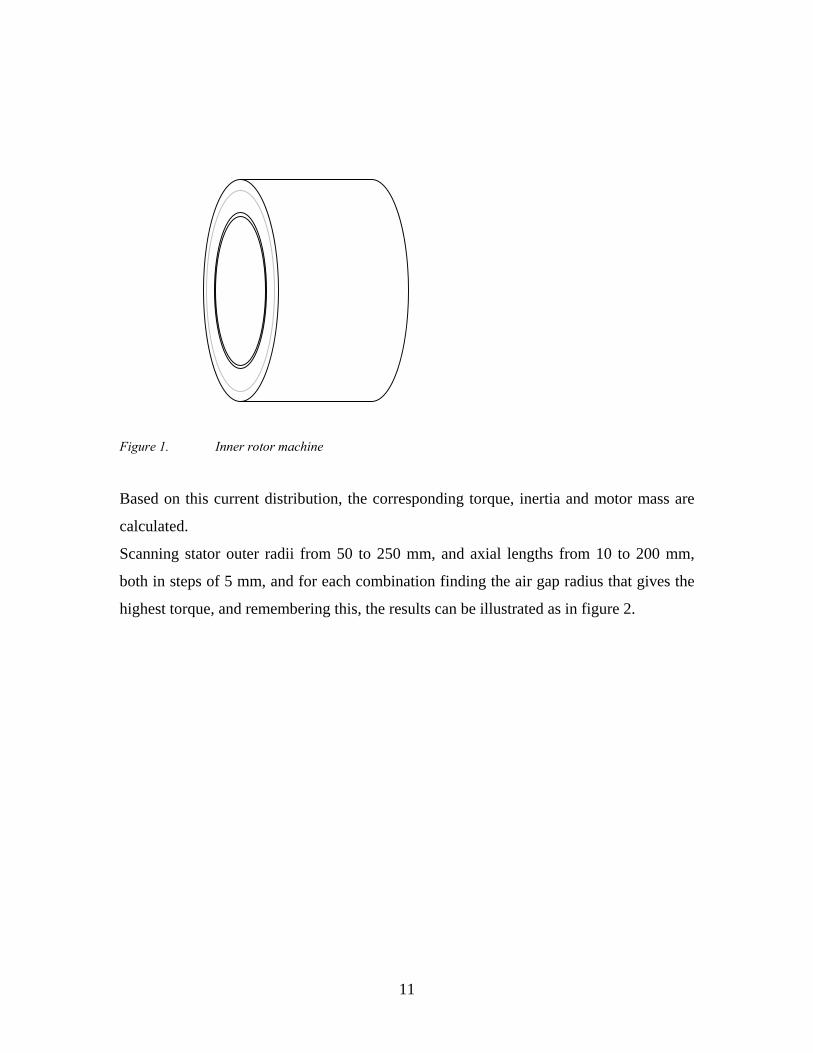
Figure 1. Inner rotor machine

Based on this current distribution, the corresponding torque, inertia and motor mass are

calculated.

Scanning stator outer radii from 50 to 250 mm, and axial lengths from 10 to 200 mm,

both in steps of 5 mm, and for each combination finding the air gap radius that gives the

highest torque, and remembering this, the results can be illustrated as in figure 2.

11

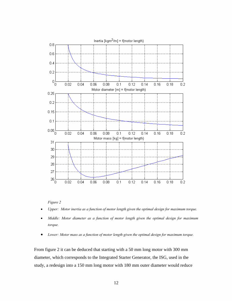
Figure 2

• Upper: Motor inertia as a function of motor length given the optimal design for maximum torque.

• Middle: Motor diameter as a function of motor length given the optimal design for maximum

torque.

• Lower: Motor mass as a function of motor length given the optimal design for maximum torque.

From figure 2 it can be deduced that starting with a 50 mm long motor with 300 mm

diameter, which corresponds to the Integrated Starter Generator, the ISG, used in the

study, a redesign into a 150 mm long motor with 180 mm outer diameter would reduce

12

the motor inertia a factor of 3, without changing the mass significantly. This also states

that the acceleration and deceleration could be cut by almost the same factor.

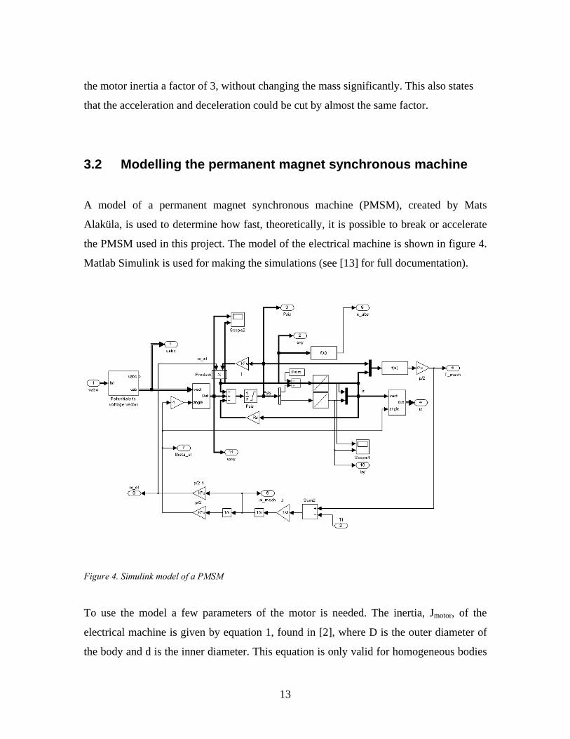
3.2 Modelling the permanent magnet synchronous machine

A model of a permanent magnet synchronous machine (PMSM), created by Mats

Alaküla, is used to determine how fast, theoretically, it is possible to break or accelerate

the PMSM used in this project. The model of the electrical machine is shown in figure 4.

Matlab Simulink is used for making the simulations (see [13] for full documentation).

Figure 4. Simulink model of a PMSM

To use the model a few parameters of the motor is needed. The inertia, Jmotor, of the

electrical machine is given by equation 1, found in [2], where D is the outer diameter of

the body and d is the inner diameter. This equation is only valid for homogeneous bodies

13

and not applicable in this case, however by disassembling the motor in four parts four

homogeneous bodies were obtained. The inner diameter of the first part has been

measured to 268 mm, the outer diameter to 283 mm and the mass to 5 kg. Second part

measured 268 mm outer and 39 mm inner diameter with a mass of 6 kg. Third part

112mm outer and 40 mm inner diameter with a mass of 3 kg. Last part was the clutch

plate, which weighs 2 kg with an outer diameter of 238 mm and an inner diameter of

28mm. Equation 2 gives the inertia of the electrical machine.

8

22 dDmJ += (1)

22222

222222

0.1778kgm8

028.0238.0*3.28

040.0112.0*0.3

8039.0283.0*0.6

8268.0283.0*0.5

8

=+

++

+

++

+=

+=

dDmJ motor

(2)

The motor is at all times connected to the incoming shaft of the gearbox and the inertia of

this shaft must be added to the total inertia. The shaft holds six gears with an average

outer diameter of 0.1m, an average inner diameter of 0.044m and an average weight of

0.5kg. The shaft itself weighs 0.62kg and has a diameter of 20mm. The total inertia of the

incoming shaft can then be calculated using equation 3.

222

2222

0.0022kgm16

044.01.0*

5.0*61602.0*62.0

16*6

16

=+

+=+

+= geargeargear

shaftshaftshaft

dDm

DmJ

(3)

The total inertia, J, is the sum of Jmotor and Jshaft. J= Jmotor + Jshaft = 0.18kgm2

Since the electrical machine came with very few data most of the motor parameters has

been experimentally determined. To resolve the linked magnetic flux, Ψm, an

14

oscilloscope was attached to two of the phases and the motor was turned over manually.

By measuring the peak-to-peak voltage and the frequency the linked magnetic flux can be

calculated using equation 3 (from [1]). In the equation the angular velocity and the root

mean square value of the voltage are needed which easily can be calculated from the

frequency and the peak-to-peak voltage. The peak-to-peak voltage was measured to

7.92V for 38.17Hz.

0.0117pi*2*38.17

27.92/2/===Ψ

ωh

mU

(4)

From the electrical machine's rated power, 10kW, the rated torque, T and the rated

current in the q-direction, isy,n, are determined. In equation 5 (also from [1]) the rated

torque is calculated. The maximum voltage vector that the power converter can give is

2/max UdcU = . Where Udc is 42V.

(RMS)currentphaseA192310000max

U

/ I n ==

currentvectorpeakA3333 == nsyn *II (5)

torquemechanical nominal 81.7Nm2

==p**IΨT synm

1170rpmrad/s1227.81

104

====n

ubase T

Pω

The stator inductance is measured to 0.0495mH and assumed to be the same in both x-

and y-directions. The stator resistance was measured using the four wire method

15

described in appendix B, found in [3] and [4] and was measured to 0.00625ohm. The

number of poles of the machine used was 42 and the motor is designed for a 36V system.

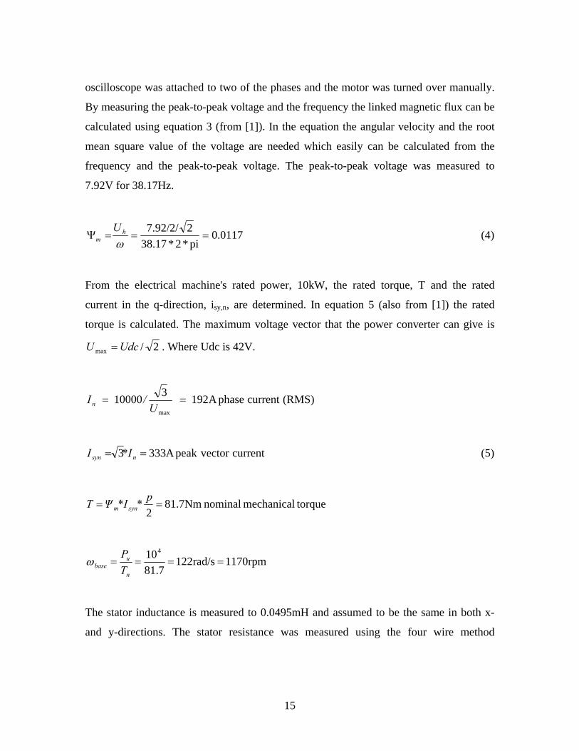
A sampled vector controller as described in [1] has been added to the model of the

PMSM and is used for controlling the motor. The model of the vector controller is shown

in figure 5.

Figure 5. Simulink model of a PI sampled vector controller.

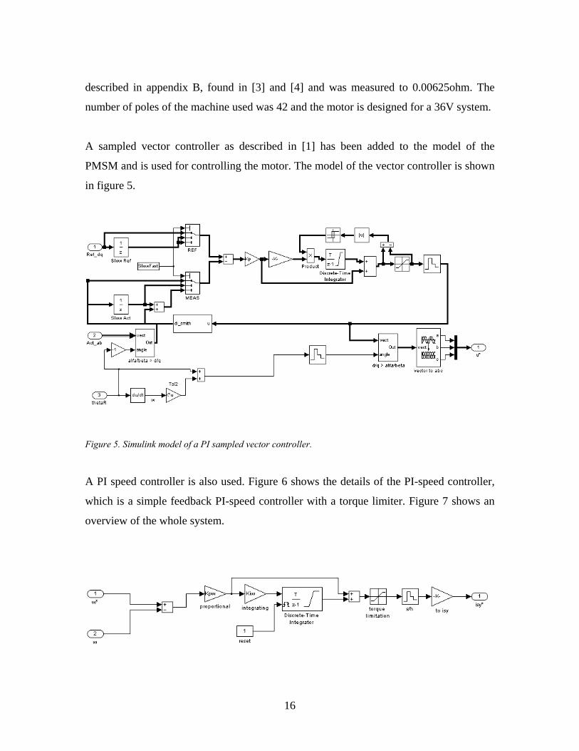
A PI speed controller is also used. Figure 6 shows the details of the PI-speed controller,

which is a simple feedback PI-speed controller with a torque limiter. Figure 7 shows an

overview of the whole system.

16

Figure 6. The PI-speed controller.

Figure 7. Overview of the full Simulink model.

The last block, called the average voltage amplifier models the behaviour of the power

electronics used for controlling the PMSM. The details of this block are shown in figure

8.

17

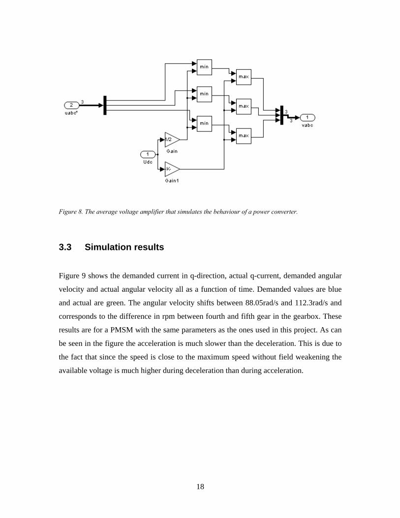
Figure 8. The average voltage amplifier that simulates the behaviour of a power converter.

3.3 Simulation results

Figure 9 shows the demanded current in q-direction, actual q-current, demanded angular

velocity and actual angular velocity all as a function of time. Demanded values are blue

and actual are green. The angular velocity shifts between 88.05rad/s and 112.3rad/s and

corresponds to the difference in rpm between fourth and fifth gear in the gearbox. These

results are for a PMSM with the same parameters as the ones used in this project. As can

be seen in the figure the acceleration is much slower than the deceleration. This is due to

the fact that since the speed is close to the maximum speed without field weakening the

available voltage is much higher during deceleration than during acceleration.

18

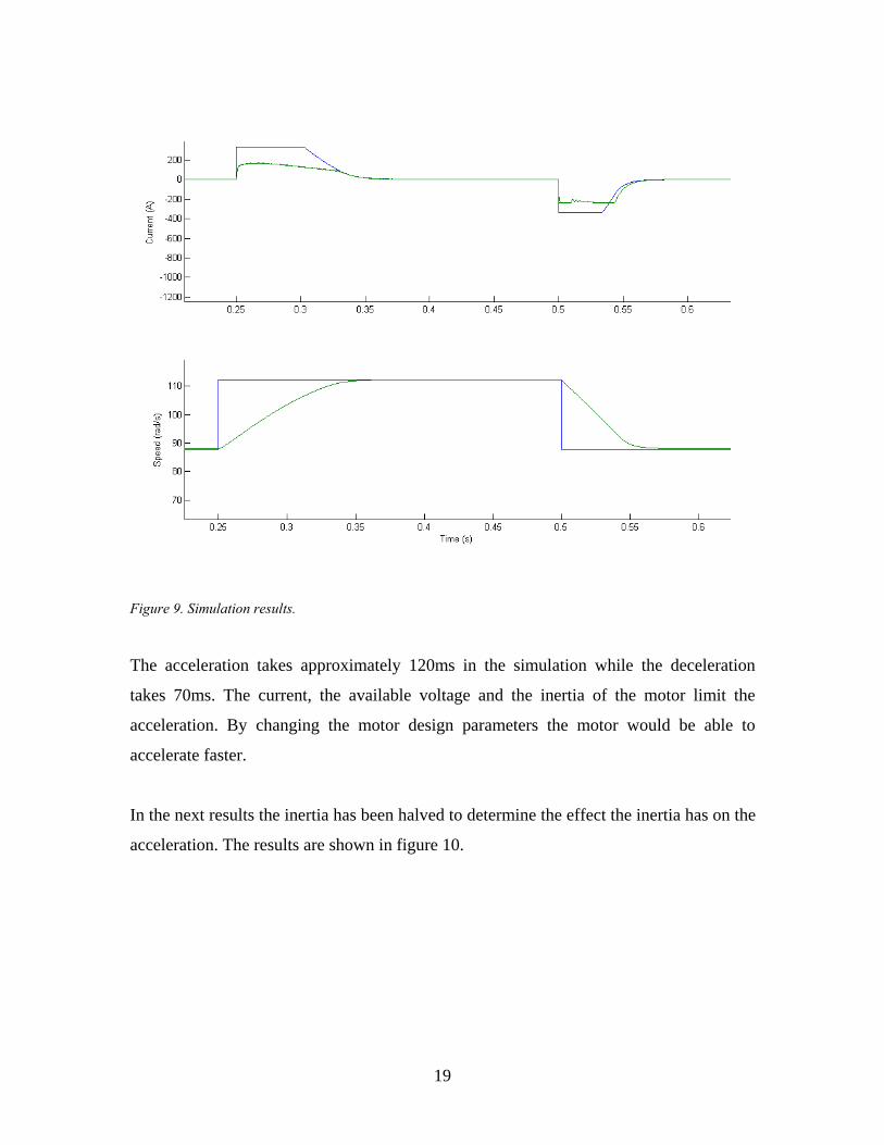
Figure 9. Simulation results.

The acceleration takes approximately 120ms in the simulation while the deceleration

takes 70ms. The current, the available voltage and the inertia of the motor limit the

acceleration. By changing the motor design parameters the motor would be able to

accelerate faster.

In the next results the inertia has been halved to determine the effect the inertia has on the

acceleration. The results are shown in figure 10.

19

Figure 10. Simulation results with inertia halved.

As shown in figure 10, by cutting the inertia to half the acceleration time is also halved.

This states the importance of a correct design of the traction motor. A motor with

sufficient amount of torque and power is needed to be able to drive the car only using the

electric traction motor but a small enough motor not to lose the ability to accelerate fast

during gearshift.

20

3.4 The gear shifting sequence

The gear shifting sequence consists of five different states as described in figure 11.

Figure 11. Block scheme of the gear shifting sequence.

1. Setting the torque to zero means removing the torque from the input shaft by

setting all currents to zero, which takes approximately one sample period.

2. The time for putting the gearbox into neutral is limited by the inertia of the

actuator used for controlling the gear stick, the inertia of the shafts, moving the

gears in the gearbox and the power and forces of the actuator.

3. The speed synchronisation is done by the traction motor and is limited by the

inertia in the traction motor, the inertia in the shafts in the gearbox, the torque in

the electrical machine and the available current. The dynamical and static

parameters of the traction motor are described in 3.2.

4. Shifting gear is done by the gear-shifting robot and is limited by the same

parameters as when the gear is put into neutral position. Torque is reapplied

within one sample period.

Returning the gear stick to its home position is also done by the gear-shifting robot and

thus limited by the same parameters as for putting the gearbox in neutral.

21

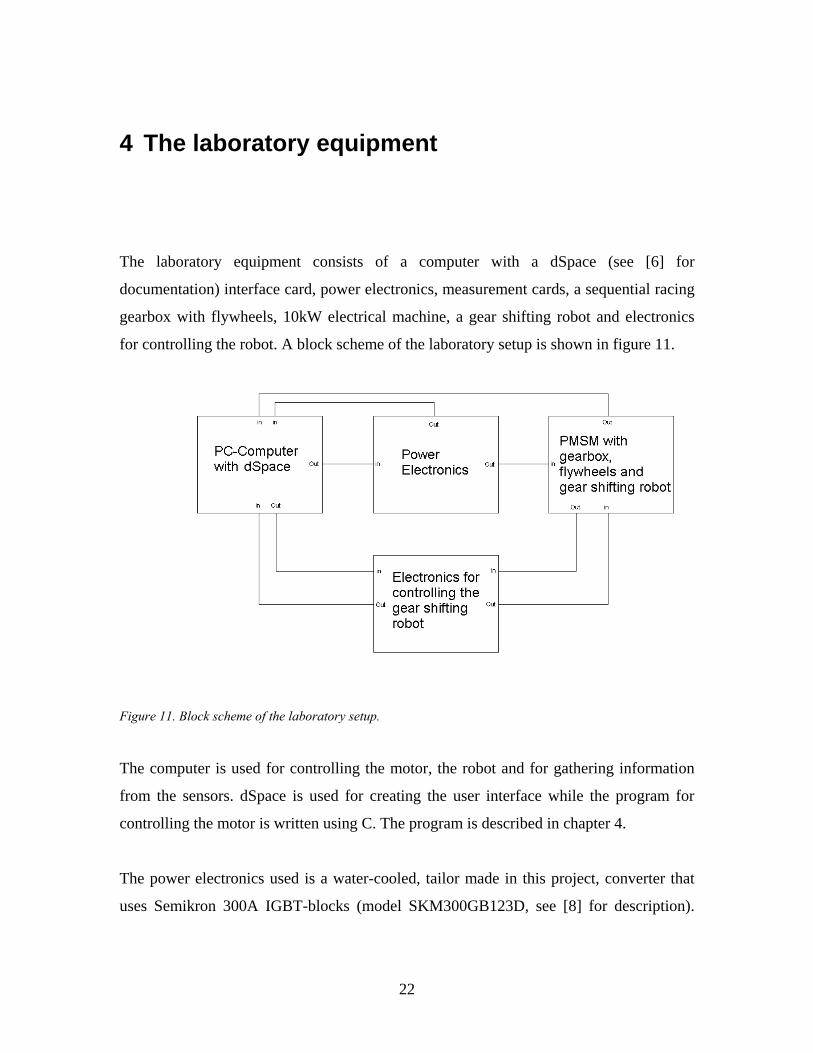
4 The laboratory equipment The laboratory equipment consists of a computer with a dSpace (see [6] for

documentation) interface card, power electronics, measurement cards, a sequential racing

gearbox with flywheels, 10kW electrical machine, a gear shifting robot and electronics

for controlling the robot. A block scheme of the laboratory setup is shown in figure 11.

Figure 11. Block scheme of the laboratory setup.

The computer is used for controlling the motor, the robot and for gathering information

from the sensors. dSpace is used for creating the user interface while the program for

controlling the motor is written using C. The program is described in chapter 4.

The power electronics used is a water-cooled, tailor made in this project, converter that

uses Semikron 300A IGBT-blocks (model SKM300GB123D, see [8] for description).

22

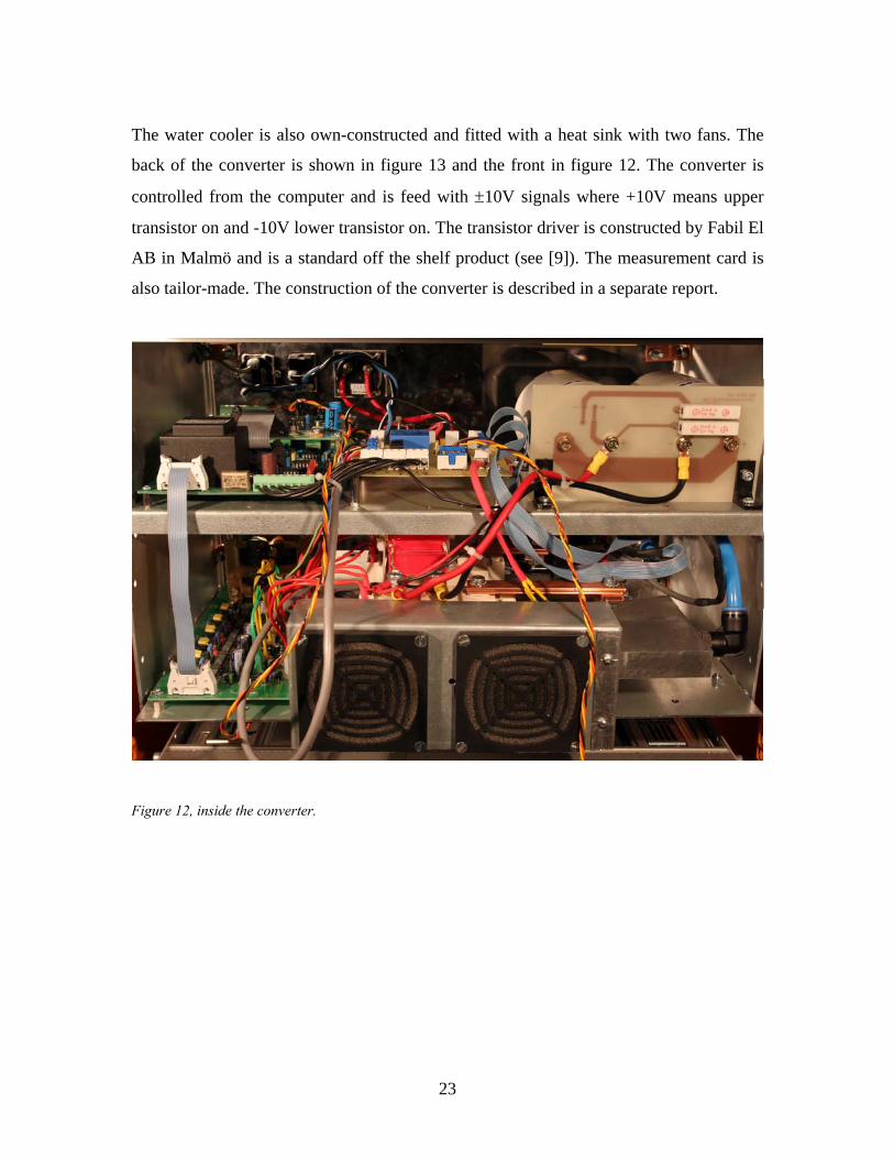
The water cooler is also own-constructed and fitted with a heat sink with two fans. The

back of the converter is shown in figure 13 and the front in figure 12. The converter is

controlled from the computer and is feed with ±10V signals where +10V means upper

transistor on and -10V lower transistor on. The transistor driver is constructed by Fabil El

AB in Malmö and is a standard off the shelf product (see [9]). The measurement card is

also tailor-made. The construction of the converter is described in a separate report.

Figure 12, inside the converter.

23

Figure 13, the front of the converter.

The gearbox is a six-gear sequential racing gearbox that has been fitted with a 10kW

permanent magnet synchronous electrical machine (PMSM). A servo for controlling the

gear stick has also been fitted to the gearbox. The gearbox is mounted in a rig and on the

outgoing shaft three 56kg flywheels has been fitted. This simulates the moving masses of

a real car. The rig is shown in figure 14.

24

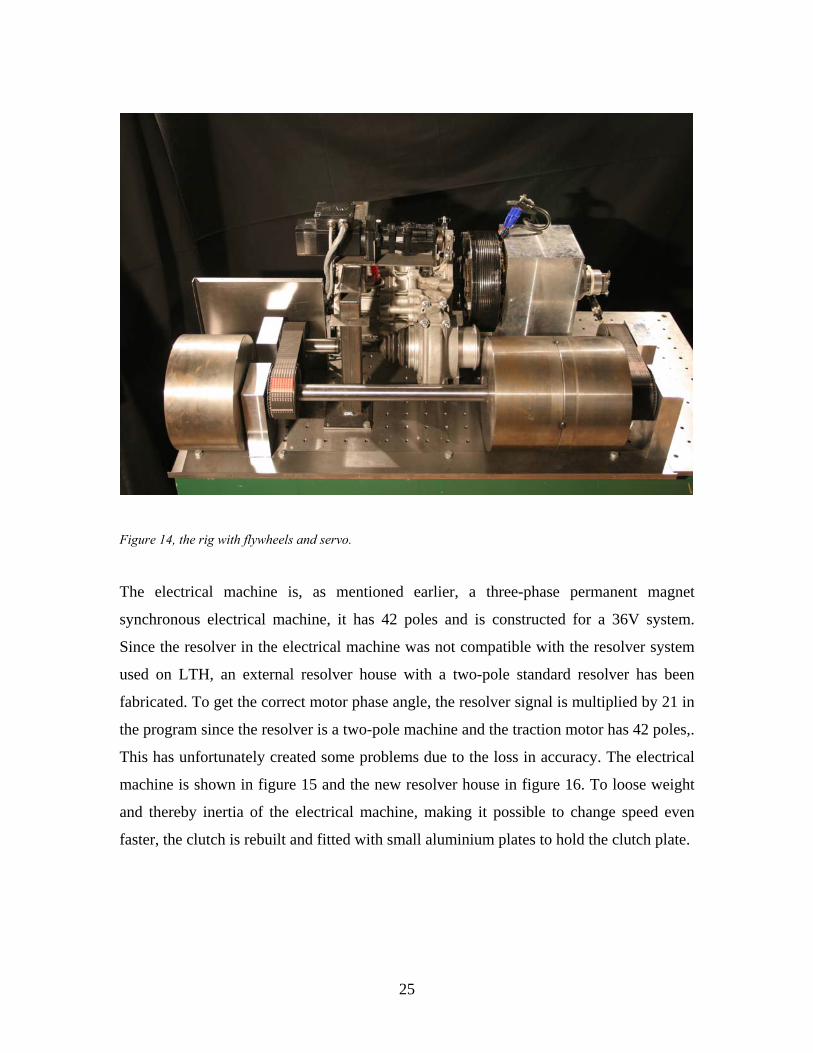
Figure 14, the rig with flywheels and servo.

The electrical machine is, as mentioned earlier, a three-phase permanent magnet

synchronous electrical machine, it has 42 poles and is constructed for a 36V system.

Since the resolver in the electrical machine was not compatible with the resolver system

used on LTH, an external resolver house with a two-pole standard resolver has been

fabricated. To get the correct motor phase angle, the resolver signal is multiplied by 21 in

the program since the resolver is a two-pole machine and the traction motor has 42 poles,.

This has unfortunately created some problems due to the loss in accuracy. The electrical

machine is shown in figure 15 and the new resolver house in figure 16. To loose weight

and thereby inertia of the electrical machine, making it possible to change speed even

faster, the clutch is rebuilt and fitted with small aluminium plates to hold the clutch plate.

25

Figure 15, the electrical machine with the custom- built clutch plate holder.

26

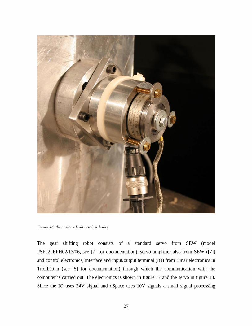
Figure 16, the custom- built resolver house.

The gear shifting robot consists of a standard servo from SEW (model

PSF222EPH02/13/06, see [7] for documentation), servo amplifier also from SEW ([7])

and control electronics, interface and input/output terminal (IO) from Binar electronics in

Trollhättan (see [5] for documentation) through which the communication with the

computer is carried out. The electronics is shown in figure 17 and the servo in figure 18.

Since the IO uses 24V signal and dSpace uses 10V signals a small signal processing

27

board that converts 10V signals to 24V and vice versa has been constructed. The

operating principles of the PCB are shown in figure 19 and the real PCB in figure 20. The

PCB uses discrete transistor technology using BD139 and BD140 (see [10] and [11])

transistors. The signal is buffered in the first step using a simple voltage-follower

(LF347F, see [12]) and then switched to the correct value using the transistors.

28

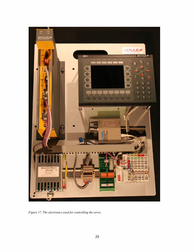
Figure 17. The electronics used for controlling the servo.

29

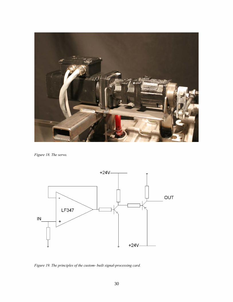
Figure 18. The servo.

Figure 19. The principles of the custom- built signal-processing card.

30

Figure 20. The custom built signal-processing card.

In figure 21 the front of the measurement boards are shown. The far left one is the power

supply, followed by the resolver board that collects signals from the resolver and converts

them, together with the sine/cosine card next to it, to sine and cosine signals and a speed

signal. Next is the current and voltage measurement board, which is not used here. The

far right card is the dSpace interface board that contains buffer and protection circuits to

provide smooth signals and to protect the dSpace processor board in the computer.

31

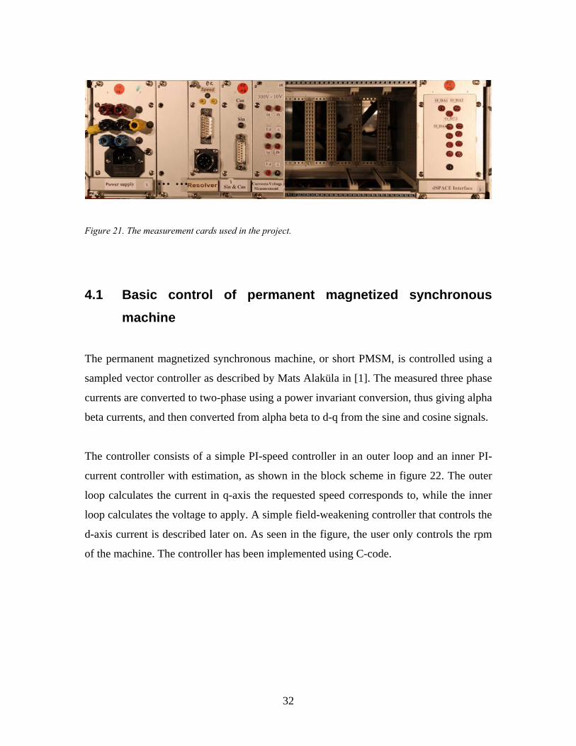
Figure 21. The measurement cards used in the project.

4.1 Basic control of permanent magnetized synchronous

machine

The permanent magnetized synchronous machine, or short PMSM, is controlled using a

sampled vector controller as described by Mats Alaküla in [1]. The measured three phase

currents are converted to two-phase using a power invariant conversion, thus giving alpha

beta currents, and then converted from alpha beta to d-q from the sine and cosine signals.

The controller consists of a simple PI-speed controller in an outer loop and an inner PI-

current controller with estimation, as shown in the block scheme in figure 22. The outer

loop calculates the current in q-axis the requested speed corresponds to, while the inner

loop calculates the voltage to apply. A simple field-weakening controller that controls the

d-axis current is described later on. As seen in the figure, the user only controls the rpm

of the machine. The controller has been implemented using C-code.

32

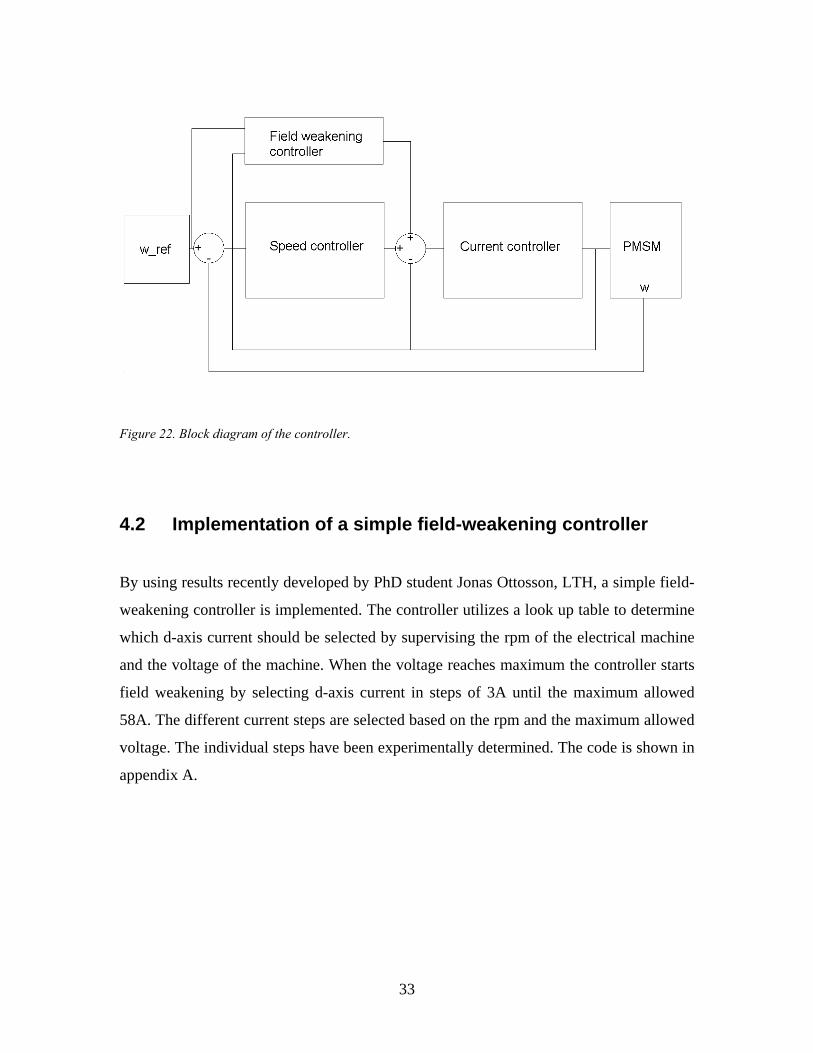
Figure 22. Block diagram of the controller.

4.2 Implementation of a simple field-weakening controller

By using results recently developed by PhD student Jonas Ottosson, LTH, a simple field-

weakening controller is implemented. The controller utilizes a look up table to determine

which d-axis current should be selected by supervising the rpm of the electrical machine

and the voltage of the machine. When the voltage reaches maximum the controller starts

field weakening by selecting d-axis current in steps of 3A until the maximum allowed

58A. The different current steps are selected based on the rpm and the maximum allowed

voltage. The individual steps have been experimentally determined. The code is shown in

appendix A.

33

4.3 Control of the gear-shifting robot

Control of the servo amplifier is taken care of by Binar's own control electronics (see

[5]). Binar's control system has a communication interface (IO) with five inputs through

which the gear shifting can be controlled. The different inputs are:

• HOME, which is used to return the gear stick to its idle position.

• FREE UP positions the gear rod in the gearbox neutral position when shifting up.

• SHIFT UP positions the gear rod in gear up position.

• FREE DOWN is neutral when shifting gear down

• SHIFT DOWN gives the position for shifting down

This means that to shift gear up the sequence: FREE UP, SHIFT UP, HOME must be

written. Shift down is: FREE DOWN, SHIFT DOWN, HOME.

In-between FREE UP and SHIFT UP respectively FREE DOWN and SHIFT DOWN the

speed of the electrical machine is reduced respectively increased thus making the

synchronisation of the incoming and outgoing axles.

To create the signals above dSpace's output and input signals are used. Since Binar's IO-

system uses a 24V-signal system and the dSpace system uses 10V signals a signal-

processing board that converts 10V-signals to 24V-signals has been implemented. This

board is described in the laboratory setup section. In the code these signals are created

using IF-topology and flags to tell in which state the gear shifting sequence is. Since the

program is more than a thousand times faster than Binar's IO-systems, delays have been

added in the code to create to the correct timings.

The gear shifting sequence consists of the five different states as described below:

34

1. First the torque of the electrical machine is set to zero by setting all currents to

zero.

2. Then the gearbox is put into neutral using FREE UP or FREE DOWN depending

on whether the program is undergoing a gear shift up or down.

3. After this the speed control is switched on and the rpm is synchronised.

4. Then the speed controller is turned off and the sequence continues with giving the

signal to put the gear stick in GEAR UP or GEAR DOWN making the gearbox

shifting gear up or down.

5. The torque controller is reactivated and the gear rod is returned to its HOME

position.

The total torque loss time is the sum of the time for putting the gearbox in neutral,

synchronisation of the speed and the time for making the gear rod shift gear. In figure

23 the sequence can be seen as a block scheme and in figure 24 the sequence can be

seen as it is in the computer interface. The numbers correspond to the different states

in the program. 1 is the time for putting the gear rod in neutral, 2 the time of speed

synchronisation, 3 the time for putting the gear box in gear, 4 a delay time before 5,

returning the rod in HOME position, can be carried out.

Figure 23. Block scheme of the gear shifting sequence.

35

Figure 24. A typical gear shifting sequence from the computer interface.

4.4 A short description of the computer program

The original program was written in C by PhD student Thomas Berg and intended for

controlling a PMSM, but only very few lines of the original code remains. The first

section is used for variable declaration. The next section is used for sampling data from

the current and voltage sensors, the sine and cosine signals, angular velocity and the rotor

angle. The sine, cosine and angular velocity signals are all derived from the resolver

signal while the rotor angle is calculated from the sine and cosine signals. After this

follows a section used for shifting gears and speed synchronisation. In the last section the

controller, as described in "4.1 Basic control of a permanent magnet synchronous

machine" and "4.2 Implementation of a simple field-weakening controller, has been

implemented. The code is compiled and downloaded on the DSP on the dSpace card in

the computer. The program on the card then communicates with dSpace using internal

wiring in the computer. The processor in the computer is only used for handling the

graphic interface used by the user, all of the time critical code runs on the DSP. All of the

code can be found in appendix A where some minor comments on the code can be found.

36

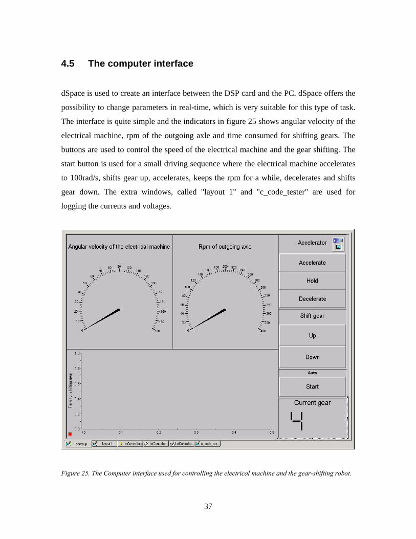
4.5 The computer interface

dSpace is used to create an interface between the DSP card and the PC. dSpace offers the

possibility to change parameters in real-time, which is very suitable for this type of task.

The interface is quite simple and the indicators in figure 25 shows angular velocity of the

electrical machine, rpm of the outgoing axle and time consumed for shifting gears. The

buttons are used to control the speed of the electrical machine and the gear shifting. The

start button is used for a small driving sequence where the electrical machine accelerates

to 100rad/s, shifts gear up, accelerates, keeps the rpm for a while, decelerates and shifts

gear down. The extra windows, called "layout 1" and "c_code_tester" are used for

logging the currents and voltages.

Figure 25. The Computer interface used for controlling the electrical machine and the gear-shifting robot.

37

5 Results 5.1 Experimental results

All results have been derived from the computer interface and from figures like figure 25

in the “Control of gear shifting robot” section. The time unit in all tables and charts in

these sections are milliseconds. The letter A in table 1 corresponds to the time to put the

gearbox in neutral. B is the time used for speed synchronisation. C is the time for putting

the gearbox in gear. D is a delay time necessary because of the response time in Binar's

system. E is the time for returning the gear stick to its home position. This means that the

total torque loss time for one gearshift corresponds to the total sum of A+B+C.

5.2 Early results

The first tests that were performed on the system were simple up and down shifts

between the fourth and the fifth gear. At this point the system were not in any way

optimised. The converter used at this time was only able to deliver 100A of current,

corresponding to about 50 % of the motors nominal current. Further, the gear shifting-

servo was not fully optimised for the system. Each experiment is divided into two

different steps, one for shifting up and one for shifting down.

38

5.2.1 Shifting up

Table 1 contains the results from ten measurement cycles when shifting from fourth to

fifth gear. The mean results have been plotted in figure 26.

Shift Up

Drive 1 2 3 4 5 6 7 8 9 10

A (Shift to neutral) 220 230 210 230 220 220 220 230 210 210

B (Synch. of speed) 300 300 300 300 300 300 300 300 300 300

C (Shift into gear) 230 210 220 210 230 220 220 210 220 230

D (Delay time) 30 30 30 30 30 30 30 30 30 30

E (Bring lever to home) 230 230 210 230 230 230 230 230 210 230

Sum 1010 1000 970 1000 1010 1000 1000 1000 970 1000

Torque loss 750 740 730 740 750 740 740 740 730 740

Mean torque loss 740

Table 1. Results from ten different cycles when shifting from fourth to fifth gear. All results in milliseconds.

39

Mean times for shifting from fourth to fifth gear

220

300

220

30

226

996

740

0

200

400

600

800

1000

1200

Gear out (A) Speedsynchronizat ion (B)

Gear in (C) Delay t ime f or servo(D)

Homing of t he servo(E)

Sum Torque loss

Figure 26. The mean results from ten cycles when shifting from fourth to fifth gear. All results in

milliseconds.

5.2.2 Shifting down

In the same manner the downshifting times are measured and the results are presented in

Table 2 and in figure 27.

Shift Down

Drive 1 2 3 4 5 6 7 8 9 10

A 120 100 100 110 100 100 100 110 100 110

B 110 120 120 120 120 120 110 100 110 110

C 100 110 100 100 110 100 100 120 100 100

D 25 25 25 25 25 25 25 25 25 25

E 110 110 110 120 110 110 120 10 120 110

Sum 465 465 455 475 465 455 455 365 455 455

Torque loss 330 330 320 330 330 320 310 330 310 320


Table 2. Results from ten drives when shifting from fifth to fourth gear. All results in milliseconds.

40

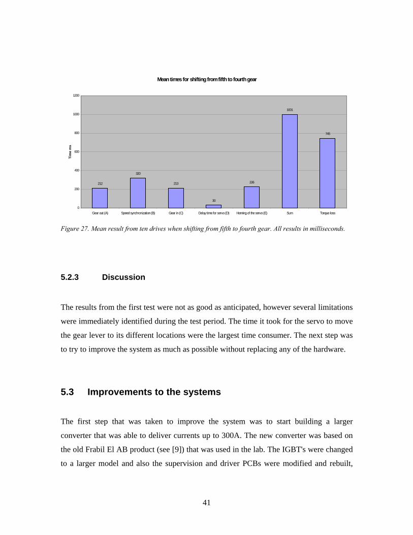
Mean times for shifting from fifth to fourth gear

212

320

213

30

226

1001

745

0

200

400

600

800

1000

1200

Gear out (A) Speed synchronization (B) Gear in (C) Delay time for servo (D) Homing of the servo (E) Sum Torque loss

Tim

e m

s

Figure 27. Mean result from ten drives when shifting from fifth to fourth gear. All results in milliseconds.

5.2.3 Discussion

The results from the first test were not as good as anticipated, however several limitations

were immediately identified during the test period. The time it took for the servo to move

the gear lever to its different locations were the largest time consumer. The next step was

to try to improve the system as much as possible without replacing any of the hardware.

5.3 Improvements to the systems

The first step that was taken to improve the system was to start building a larger

converter that was able to deliver currents up to 300A. The new converter was based on

the old Frabil El AB product (see [9]) that was used in the lab. The IGBT's were changed

to a larger model and also the supervision and driver PCBs were modified and rebuilt,

41

and also the cooling of the IGBT’s was redesigned. Further contact was taken with Binar

AB that delivered the servo, in order to let them trim the servo to its peak performance.

The clutch assembly that was mounted on the traction motor was also removed to lighten

the flywheel and lessen the inertia. Also the C code was optimised and partly rewritten to

suit the new system.

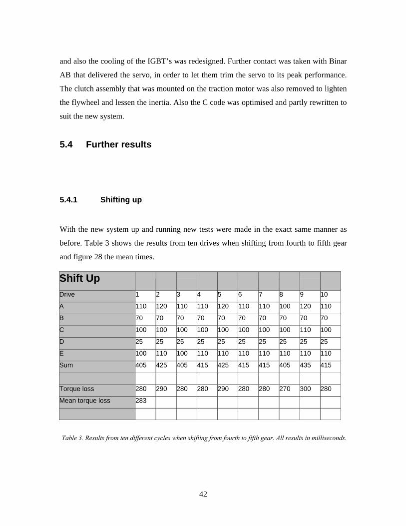
5.4 Further results

5.4.1 Shifting up

With the new system up and running new tests were made in the exact same manner as

before. Table 3 shows the results from ten drives when shifting from fourth to fifth gear

and figure 28 the mean times.

Shift Up

Drive 1 2 3 4 5 6 7 8 9 10

A 110 120 110 110 120 110 110 100 120 110

B 70 70 70 70 70 70 70 70 70 70

C 100 100 100 100 100 100 100 100 110 100

D 25 25 25 25 25 25 25 25 25 25

E 100 110 100 110 110 110 110 110 110 110

Sum 405 425 405 415 425 415 415 405 435 415

Torque loss 280 290 280 280 290 280 280 270 300 280


Table 3. Results from ten different cycles when shifting from fourth to fifth gear. All results in milliseconds.

42


112

70

101

25

108

416

283

0

50

100

150

200

250

300

350

400

450




Sum Torque loss

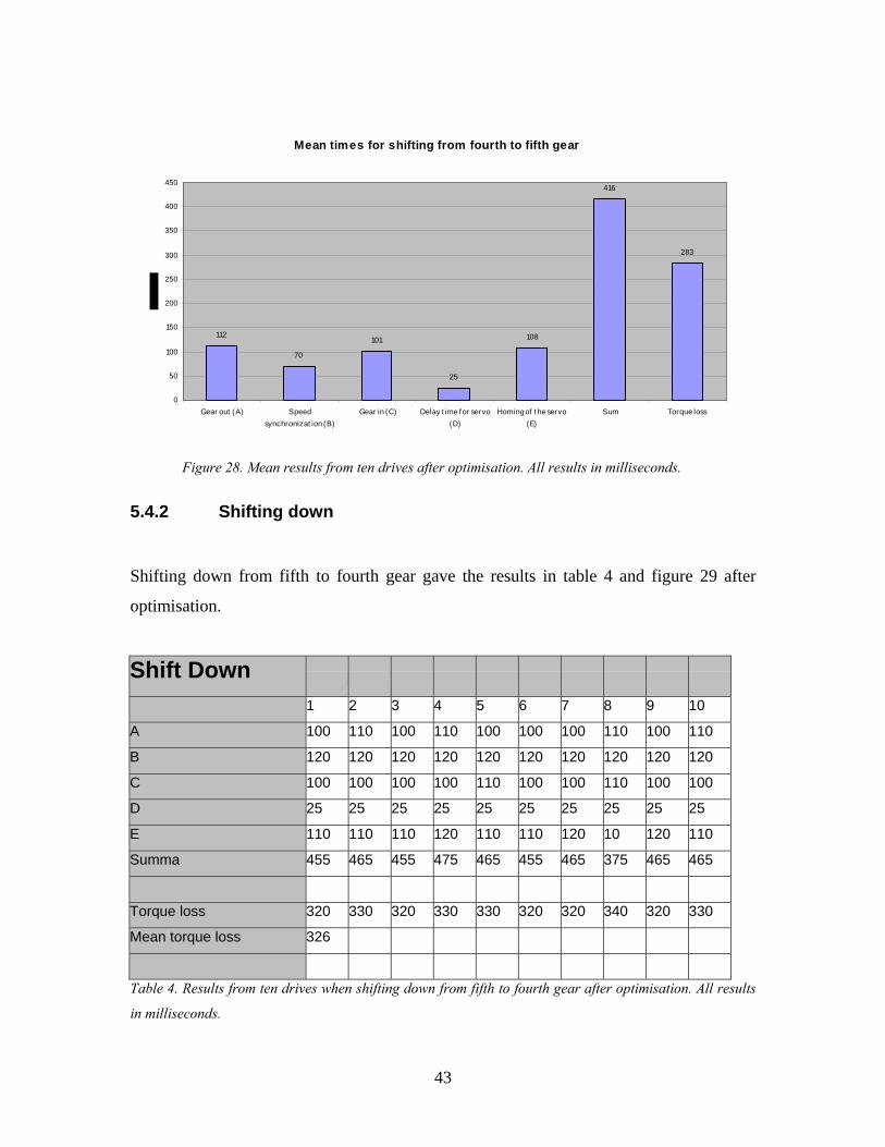
Figure 28. Mean results from ten drives after optimisation. All results in milliseconds.

5.4.2 Shifting down

Shifting down from fifth to fourth gear gave the results in table 4 and figure 29 after

optimisation.

Shift Down

1 2 3 4 5 6 7 8 9 10

A 100 110 100 110 100 100 100 110 100 110

B 120 120 120 120 120 120 120 120 120 120

C 100 100 100 100 110 100 100 110 100 100

D 25 25 25 25 25 25 25 25 25 25

E 110 110 110 120 110 110 120 10 120 110

Summa 455 465 455 475 465 455 465 375 465 465

Torque loss 320 330 320 330 330 320 320 340 320 330


Table 4. Results from ten drives when shifting down from fifth to fourth gear after optimisation. All results

in milliseconds.

43


104120

102

25

103

454

326

0

50

100

150

200

250

300

350

400

450

500




Sum Torque loss

Figure 29. Mean times when shifting down from fifth to fourth gear after optimisation. All results in

milliseconds.

5.4.3 Discussion

The results of these tests started to show the potential of the full system according to the

expectations that was set up at the start of the project. The times for shifting gears were a

factor three faster than the initial values. Both the synchronisation of the traction motor

and the gear-lever servo were improved in speed. Also the accuracy of the

synchronisation was improved so that the engagement of the gears is almost seamless.

During the tests it was argued whether the gear-lever servo could be improved in speed

further. The return spring in the gearbox was identified to be to stiff and thought to

reduce the speed of the servo why the gearbox was finally sent back to SAAB in

Trollhättan to undergo some minor adjustments. The return spring was removed from the

gear stick and the gearbox was fully disassembled.

44

5.5 Final results

The following results were the results obtained after having trimmed the equipment as far

as possible without changing any of the hardware.

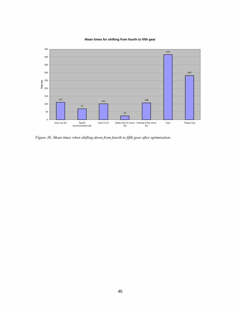
5.5.1 Shifting up

With the new system up and running new tests were made in the exact same manner as

before. Table 5 shows the results from ten drives when shifting from fourth to fifth gear

and figure 30 the mean times

Shift Up

Drive 1 2 3 4 5 6 7 8 9 10

A 100 110 100 110 110 100 110 100 120 110

B 70 70 70 70 70 70 70 70 70 70

C 110 110 100 100 110 100 100 100 110 100

D 25 25 25 25 25 25 25 25 25 25

E 100 110 100 110 110 110 110 110 110 110

Sum 405 425 395 415 425 405 415 405 435 415

Torque loss 280 290 270 280 290 270 280 270 300 280


Table 5. Results when shifting from fourth to fifth gear after gearbox adjustments

45


112

70

101

25

108

416

283

0

50

100

150

200

250

300

350

400

450

Gear out (A) Speedsynchronization (B)

Gear in (C) Delay time for servo(D)

Homing of the servo(E)

Sum Torque loss

Tim

e m

s

Figure 30. Mean times when shifting down from fourth to fifth gear after optimisation.

46

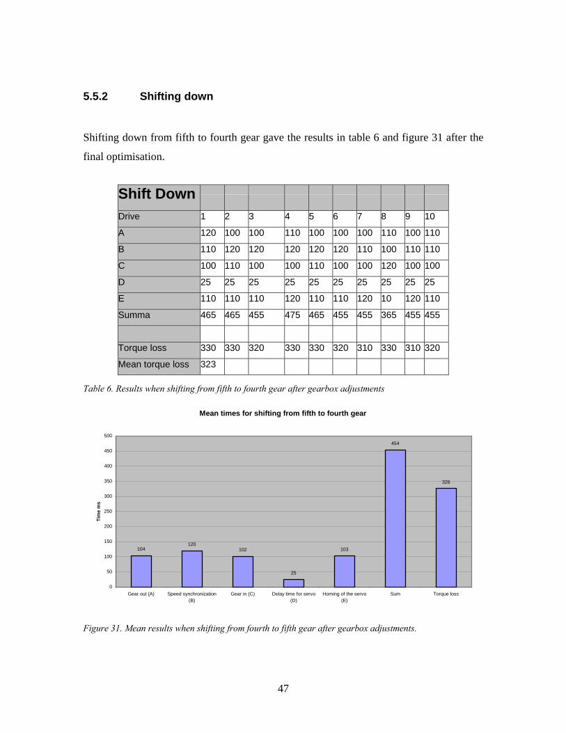
5.5.2 Shifting down

Shifting down from fifth to fourth gear gave the results in table 6 and figure 31 after the

final optimisation.

Shift Down

Drive 1 2 3 4 5 6 7 8 9 10

A 120 100 100 110 100 100 100 110 100 110

B 110 120 120 120 120 120 110 100 110 110

C 100 110 100 100 110 100 100 120 100 100

D 25 25 25 25 25 25 25 25 25 25

E 110 110 110 120 110 110 120 10 120 110

Summa 465 465 455 475 465 455 455 365 455 455

Torque loss 330 330 320 330 330 320 310 330 310 320


Table 6. Results when shifting from fifth to fourth gear after gearbox adjustments


104120

102

25

103

454

326

0

50

100

150

200

250

300

350

400

450

500

Gear out (A) Speed synchronization(B)

Gear in (C) Delay time for servo(D)

Homing of the servo(E)

Sum Torque loss

Tim

e m

s

Figure 31. Mean results when shifting from fourth to fifth gear after gearbox adjustments.

47

5.5.3 Discussion

As can be seen above the modifications made no major difference in the shifting times.

This is most probably because of that the rotor to inertia ratio of the servomotor is the

major limiting factor for why the servo cannot move any faster. Tests with the servo

disconnected from the gearbox shows exactly this. In section 7, conclusions and

recommendations, guidelines for selecting another servo are given.

48

6 Discussion As can be seen in the results most of the time consumed for shifting a gear is time for

moving the servo arm. More than 80% of the total time is here. Only 15% of the time is

the speed synchronisation, the rest is communication times. It is also interesting to see

that trimming the servo can reduce the servo moving times. Comparing the first results

with the last, the servo times has been reduced by more than fifty percent. By introducing

another, faster servo and a more powerful servo amplifier, the times should be able to be

cut even more. The rotor to inertia ratio is the main limitation of the servo, and the

parameter that sets the minimum shifting time. The rotor to inertia ratio is due to the

rotor's inertia, and a smaller servo is therefore to be preferred.

As seen in the simulation results choosing a system optimal PMSM is very important. By

choosing an optimal motor the speed synchronisation times could be cut by a factor three

of what they are in this project.

The last time consumer, communications, could be optimised by choosing another

communications interface or by altering the system topology. Binar’s new system

(BiFas60, found in [5]) is much faster than the system used in this project. The system

used in this system requires 10ms pulses to react while the new system only requires 1ms

pulses. By introducing the new system, 50-60ms of the total gear shifting time could be

cut.

A problem during the project was that the neutral between the gears in the gearbox where

at different positions. Since Binar’s system only has five inputs only two gears are

available at a time in this project. An optimised gearbox should have the neutral at the

same position at all gears to keep the program as small and simple as possible.

49

By summarizing the theoretical and expected results this would give a total gear shifting

time of less than 100ms, which is below the time that a human being can perceive and

still maintaining comfort. In a four wheel driven car with electrical four wheel drive it

would be possible to compensate the torque loss with the rear-axle traction motor while

shifting gears, which would mean that there are no torque loss what so ever.

An interesting experiment would be to let the PMSM break and accelerate the

combustion engine during a gearshift. If the clutch between the electrical machine and the

combustion engine were kept closed during a gearshift the PMSM would be able to

synchronise the speed of both machines with the speed of the outgoing axle. This would

reduce the total time of a gearshift and reduce the total torque loss to a minimum.

Keeping the clutch closed would require some sort of controlled valves in the combustion

engine so that the combustion engine could help the electrical machine to reduce the

speed by applying compression or help the electrical machine accelerate by keeping all

valves opened without compression. Even without controllable valves but with accurate

speed control of the combustion engine both machines would be able to corporate in

order to reach the correct rpm in very little time.

50

7 Conclusions and recommendations 7.1 Optimised gearbox

The gearbox should have the same relatively gear ratio between all gears and have at least

seven or eighth gears to keep the rpm difference between the gears as low as possible.

Since the synchronisation rings are no longer needed they can be removed in order to

make the gearbox smaller and be able to hold more gears.

Further, a sensor that tells which gear is currently chosen is needed and a tachometer of

the outgoing axle to make the synchronisation even smoother and to be able to

compensate if the car is moving on steady ground, downwards a steep slope or upwards a

steep slope.

7.1.1 Optimal PMSM

As seen in the simulations, the PMSM should be large enough to produce sufficient

torque to move the car but small enough to be able to break or accelerate in the given

time window. By redesigning the motor to be 180mm in diameter and 150mm long, the

torque would be unaltered but the inertia, and thereby acceleration and deceleration,

would be cut by a factor of three.

51

7.1.2 System optimisation

In order to make benefit of the fact that the electrical machine has high torque at low

speed, a rather different gear shifting strategy should be used. Since the parallel hybrid

topology offers the possibility to have the combustion and electrical machine operating

together, the sum of the torque curves for both machines is rather different from the

torque curve of the combustion engine alone. Figure 32 shows typical torque curves for a

supercharged combustion engine, a PMSM and the sum of both machines. As seen in the

figure the maximum torque for both machines is at a much lower speed than of the

combustion engine alone. This means that an optimal gear shifting strategy would be to

shift gear just above torque maximum for both machines which is somewhere around

3000rpm. Doing so would imply that the car only exceeds 3000 rpm at highest gear.

Another benefit with this strategy is that the specific fuel consumption of the combustion

engine is at its lowest at all time during normal use of the car.

52

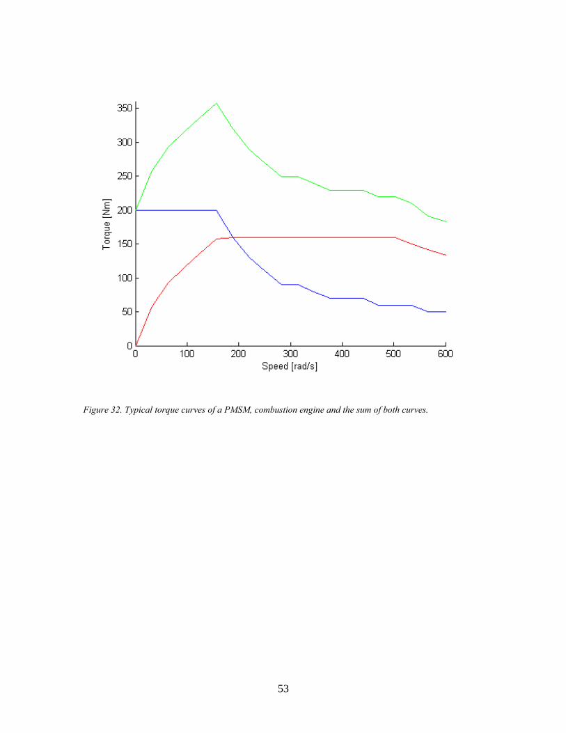
Figure 32. Typical torque curves of a PMSM, combustion engine and the sum of both curves.

53

8 References [1] M. Alaküla: Power Electronic Control, 2003

[2] Ingelstam, Rönngren, Sjöberg: TEFYMA, 1999, ISBN 91-87234-13-0

[3] P. Carlsson, S. Johansson: Modern Elektronisk Mätteknik, 2000, ISBN 91-47-

01098-3

[4] Four wire measurement

http://www.neon.co.uk/campus/articles/hp/hp9.htm

[5] Binar Electronics in Trollhättan

http://www.binar.se

[6] dSpace GmbH

http://www.dspace.de/ww/en/pub/start.cfm

[7] SEW Eurodrive

http://www.sew.de/deutsch/index.html

[8] Semikron GmbH

http://www.semikron.com

[9] Frabil El AB

http://www.frabil.se/

54

[10] BD139

http://www.elfa.se/elfa-bin/dyndok.pl?dok=2441.htm

[11] BD140


[12] LF347F


[13] Mathworks

http://www.mathworks.com/

55

Appendix A /****************************************************************************** * * FILE: * 1stController.c * * RELATED FILES: * Brtenv.h * * DESCRIPTION: Initialization and repeated duty cycle update * of PWM. Duty cycle update once per PWM period. * For updating the duty cycle the PWM Interrupt from the * Slave DSP to the Master PPC is used. * Used functions are: * * ds1104_slave_dsp_communication_init * ds1104_slave_dsp_pwm3_init * ds1104_slave_dsp_pwm3_start * ds1104_slave_dsp_pwm3_duty_write_register * ds1104_slave_dsp_pwm3_duty_write * * For the shared IO pins see RTLib Reference. * ******************************************************************************/ #include <brtenv.h> /* basic real-time environment */ #include <math.h> #include <io1104.h> /*---------------------------------------------------------------------------*/ #define PI 3.141592654 #define TwoPi 6.28318530717959 #define Sqrt_three 1.732050808 #define Sqrt_two 1.414213562 #define Sqrt_six 2.44948974278318 /* variables for communication with Slave DSP */ Int16 task_id = 0; /* communication channel */ Int16 index = -1; /* slave DSP command index */ /* parameters for PWM initialization */ Float64 period = 7.14e-5; /* PWM period */ Float64 Ts = 7.14e-5; Float64 deadband = 0.0; //lookup time-unit /* deadband period */ Float64 sync_pos = 0.5; /* position of the synch. interrupt signal 0.5: gives interrupt on the top of the tri-wave*/ /* parameters accessed by ControlDesk */

56

volatile Float64 Udc = 0; volatile Float64 w_set = 0; volatile Float64 w = 0; volatile Float64 isx_set = 0; volatile Float64 isx = 0; volatile Float64 isy_set = 0; volatile Float64 isy = 0; volatile Float64 exec_time; /* execution time */ volatile Float64 ia = 0; //phase current a volatile Float64 ib = 0; volatile Float64 ic = 0; volatile Float64 cosTheta = 1; volatile Float64 sinTheta = 0; volatile Float64 cosThetaPre = 1; volatile Float64 sinThetaPre = 0; volatile Float64 usx = 0, usy = 0,w_sum=0,w_sumold=0; volatile Float64 a = 0; volatile Float64 usy_set = 0; volatile Float64 dutyA = 0.5; volatile Float64 dutyB = 0.5; volatile Float64 dutyC = 0.5; volatile Float64 modType = 0;//0:sinusmodulation, 1:symmetrized modulation volatile Float64 angle = 0; volatile Float64 Kpc = 1.3; volatile Float64 Kis = 1; volatile Float64 Kps = 13; volatile Float64 Kic = 0.0002; volatile Float64 dQTheta = -0.80; volatile Float64 UdcTemp = 0; volatile Float64 bandrup= 0; volatile Float64 isy_setprev =0; volatile Float64 us_abs=0; volatile int mode = 0; //auto=1 manual=0 /* parameters NOT accessed by ControlDesk */ Float64 i_alpha = 0; Float64 i_beta = 0; Float64 isx_sum = 0; Float64 isy_sum = 0; Float64 isx_sumold = 0; Float64 isy_sumold = 0; Float64 usx_set = 0; Float64 u_alpha_set = 0; Float64 u_beta_set = 0; Float64 u_a_set = 0; Float64 u_b_set = 0; Float64 u_c_set = 0; Float64 L_sx = 0.1e-3; Float64 L_sy = 0.1e-3; Float64 Rs = 0.0125/2;

57

volatile Float64 Psi_m = 0.005; Float64 Kp = 0.40313*1.2;//(Rs/2+L_sy/Ts); Float64 Ki = 62.0158/1500;//(1/(L_sy/Rs+Ts/2)*10); volatile Float64 freqc = 0; volatile Float64 amp = 0; volatile Float64 c2 = 0; volatile Float64 c3 = 0; volatile Float64 c4 = 0; volatile Float64 c5 = 0; Float64 usxymax = 0; Float64 minTemp=0,maxTemp=0; volatile Float64 active=0; volatile Float64 fault = 0; volatile Float64 inpos = 0; volatile int speed=1; volatile Float64 w_setoldref = 0; volatile int whichgear = 4; volatile int shifting = 0; volatile Float64 gear=0; volatile int change=0; Float64 w_max=200; Float64 w_temp = 0; volatile int count = 0; volatile int count2 = 0; volatile int count3 = 0; volatile int count4 = 0; volatile int inposcount = 0; volatile int out1 =0; volatile int out2 =0; volatile int out3 =0; volatile int out4 =0; volatile int out5 =0; volatile int out6 =0; volatile int w_setchange=0; volatile int w_setchanged=0; volatile int w_setchange2=0; volatile int w_setchanged2=0; volatile Float64 realspeed = 0; volatile Float64 realoldspeed = 0; volatile Float64 usy_old =0; volatile Float64 isx_old_sum=0; volatile Float64 isy_old_sum=0; /*---------------------------------------------------------------------------*/ /* interrupt service routine for PWM sync interrupt */ void PWM_sync_interrupt(void){ host_service(1, 0); /* Data Acquisition service */ RTLIB_TIC_START(); /* start time measurement */ ds1104_adc_start(DS1104_ADC2|DS1104_ADC3|DS1104_ADC4|DS1104_ADC5); //do the sample

58

//ds1104_dac_init(DS1104_DACMODE_TRANSPARENT); ia = 400*ds1104_adc_read_ch(7); //read current a ib = 400*ds1104_adc_read_ch(8); //read current b ic = -ia - ib; //calc. current c cosThetaPre = ds1104_adc_read_ch(6); sinThetaPre = ds1104_adc_read_ch(5); //read rotor angle angle= 21*(atan2(cosThetaPre,sinThetaPre)+dQTheta); angle=fmod(angle,2*PI); angle=angle-PI; cosTheta = cos(angle); sinTheta = sin(angle); //Modes used for the acceleration, deceleration buttons and the manual gear shifting features if (mode==1){ mode=2; active=1.1; } if (mode==2 && w_set>=100){ mode=3; gear=1.1; } if (mode==3 && whichgear==5){ active=1.1; mode=4; } if (mode==4 && w_set>=100){ freqc=freqc+1; if (freqc>50000){ active=-1.1; mode=5; freqc=0; } } if (mode==5 && w_set<=80){ active=0; freqc=freqc+1; if (freqc>30000){ gear=-1.1; mode=0; freqc=0; } } if (w_set>w_max){ w_set=w_max; } if (whichgear==4){ //Calculates the real speed of the machine in rpm

59

realspeed=((w/TwoPi)*60)/5.8907; realspeed=realspeed*0.01+realoldspeed*0.99; realoldspeed=realspeed; } if (whichgear==5){ //Calculates the real speed of the machine in rpm realspeed=((w/TwoPi)*60)/5.0134; realspeed=realspeed*0.01+realoldspeed*0.99; realoldspeed=realspeed; } ds1104_adc_mux(2); /** Select mux channel 2, takes 1ms according help-section!*/ ds1104_adc_delayed_start(DS1104_ADC1); inpos = ds1104_adc_read_ch(2); //inpos=1; ds1104_adc_mux(4); /** Select mux channel 4, takes 1ms according help-section!*/ ds1104_adc_delayed_start(DS1104_ADC1); fault = ds1104_adc_read_ch(4); ds1104_adc_mux(1); /** Select mux channel 1, takes 1ms according help-section!*/ ds1104_adc_delayed_start(DS1104_ADC1); w = ((861*ds1104_adc_read_ch(1)-1.8)*0.002 + 0.998*w_temp);//läs in och filtrera signalen w_temp = w; ds1104_adc_mux(3); ds1104_adc_delayed_start(DS1104_ADC1); Udc = (48.2*ds1104_adc_read_ch(3))*0.01+0.99*UdcTemp; UdcTemp = Udc; i_alpha = Sqrt_three * ia / Sqrt_two; //3phase -> 2phase transformation i_beta = (ib - ic)/Sqrt_two; // Powerinvariant conversion isx = i_alpha*cosTheta + i_beta*sinTheta; //ab -> xy coordinate transformation isy = i_beta*cosTheta - i_alpha*sinTheta; //acceleration if (active>1){ freqc=1+freqc; if (freqc>1000 ){ w_set=w_set+1; freqc=0; } if (w_set>=w_max){ active=0; w_set=w_max; freqc=0; } } //section used for gear shifting and synchronisation if (w_setchange2==1){ w_set=1.187*w_setoldref;//old 1.145 }

60

if (w_setchange2==1){ if (w>=1.142*w_setoldref){ //old 1.12 w_setchange2=0; w_setchanged2=1; whichgear=whichgear-1; speed=0; } } if (count4>=1 && w_setchanged2==1){ count++; if (out6==1){ ds1104_dac_write(1,1); } if (count>1000 && inpos>0.95){ ds1104_dac_write(1,0); out6=0; count=0; count4=0; w_setchanged2=0; shifting=0; } } if (count3==1 && w_setchanged2==1){ count++; if (out5==1){ ds1104_dac_write(5,1); } if (count>1000 && inpos>0.95){ ds1104_dac_write(5,0); out5=0; count=0; count3=0; count4++; out6=1; speed=1; } } if (change==-1){ gear=0; count++; if (out4==1){ ds1104_dac_write(4,1); } if (count>1000 && inpos>0.95){ ds1104_dac_write(4,0); out4=0; count2++; // if (count2>1000){ change=0;

61

out5=1; count3++; count=0; w_setchange2=1; speed=1; // } } } if (gear<0){ w_setoldref=w_set; speed=0; w_sumold=0; isy_set=0; change=-1; out4=1; isy_setprev=0; shifting = 1; } if (w_setchange==1){ w_set=0.874*w_setoldref; } if (w_setchange==1){ if (w<=0.89*w_setoldref){ w_setchange=0; w_setchanged=1; whichgear=whichgear+1; speed=0; } } if (count4>=1 && w_setchanged==1){ count++; if (out3==1){ ds1104_dac_write(1,1); } if (count>1000 && inpos>0.95){ ds1104_dac_write(1,0); out3=0; count=0; count4=0; w_setchanged=0; shifting=0; } }

62

if (count3==1 && w_setchanged==1){ count++; if (out2==1){ ds1104_dac_write(3,1); } if (count>1000 && inpos>0.95){ ds1104_dac_write(3,0); out2=0; count=0; count3=0; count4++; out3=1; speed=1; } } if (change==1){ gear=0; count++; if (out1==1){ ds1104_dac_write(2,1); } if (count>1000 && inpos>0.95){ ds1104_dac_write(2,0); out1=0; count2++; // if (count2>1000){ change=0; out2=1; count3++; count=0; w_setchange=1; speed=1; // } } } if (gear>0){ w_setoldref=w_set; speed=0; w_sumold=0; isy_set=0; change=1; out1=1; isy_setprev=0; shifting = 1; } if (active<-1 && w_set>0) {

63

freqc=1+freqc; if (freqc>500){ w_set=w_set-1; freqc=0; //isx_set=0; if(w_set<0.1){ active=0; //isx_set=0; } } } //outer P-controller if (speed==1){ isy_set = (Kps*(w_set-w) + w_sumold);//T_set=Kp * w_diff, isy_set = T_set / Psim_SM //Current limit if(isy_set > 250){ isy_set=250; w_sum = 250 - Kis*(w_set-w); }else if(isy_set < -250){ isy_set = -250; w_sum = -250 - Kis*(w_set-w); }else{ w_sum = Kis*(w_set - w) + 0.1*w_sumold; } w_sumold = w_sum; } isy_set=0.1*isy_set+0.9*isy_setprev; //Filters the speed signal isy_setprev =isy_set; usx = Kpc*Kp*(isx_set - isx) + isx_sumold - w*L_sy*isy;//calc. controller output //field weakening controller if(usy > Udc*usxymax){ if (w_set>75 && w_set<77){ isx_set=-3; } if (w_set>77 && w_set<79){ isx_set=-6; } if (w_set>79 && w_set<81){ isx_set=-9; } if (w_set>81 && w_set<83){ isx_set=-12; } if (w_set>83 && w_set<85){ isx_set=-15; } if (w_set>85 && w_set<87){ isx_set=-18; } if (w_set>87 && w_set<89){ isx_set=-21;

64

} if (w_set>89 && w_set<91){ isx_set=-24; } if (w_set>91 && w_set<93){ isx_set=-27; } if (w_set>95 && w_set<97){ isx_set=-30; } if (w_set>99 && w_set<101){ isx_set=-33; } if (w_set>103 && w_set<105){ isx_set=-36; } if (w_set>105 && w_set<108){ isx_set=-39; } if (w_set>108 && w_set<111){ isx_set=-41; } if (w_set>111 && w_set<113){ isx_set=-43; } if (w_set>113 && w_set<115){ isx_set=-46; } if (w_set>115 && w_set<118){ isx_set=-49; } if (w_set>118 && w_set<121){ isx_set=-52; } if (w_set>121 && w_set<124){ isx_set=-55; } if (w_set>124 && w_set<127){ isx_set=-58; } } else if (w<75){ isx_set=0; } //antiwindup for usx if(usx > Udc*usxymax){ usx = Udc*usxymax; isx_old_sum = isx_sum; isx_sum = isx_old_sum;//Udc*usxymax - (Ki*Kic*(isx_set - isx)- w*L_sy*isy); }else if(usx < -Udc*usxymax){ usx = -Udc*usxymax; isx_old_sum = isx_sum; isx_sum = isx_old_sum;//-Udc*usxymax - (Ki*Kic*(isx_set - isx)- w*L_sy*isy);

65

}else{ isx_sum = Ki*Kic* (isx_set - isx) + isx_sumold; // calc. sum of differences in current } isx_sumold = isx_sum; usy = Kp*Kpc*(isy_set - isy) + /*isy_sumold */+ w*Psi_m + w*L_sx*isx;//calc. controller output //antiwindup for usy if(usy > Udc*usxymax){ usy = Udc*usxymax; isy_old_sum = isy_sum; isy_sum = isy_old_sum;//Udc*usxymax - (Ki*Kic*(isy_set - isy) + w*Psi_m + w*L_sx*isx); }else if(usy < -Udc*usxymax){ usy = -Udc*usxymax; isy_old_sum = isy_sum; isy_sum = isy_old_sum;//-Udc*usxymax - (Ki*Kic*(isy_set - isy) + w*Psi_m+ w*L_sx*isx); }else{ isy_sum = Ki*Kic*(isy_set - isy) + isy_sumold; } isy_sumold = isy_sum; us_abs=sqrt(usy*usy+usx*usx); u_alpha_set = usx*cosTheta - usy*sinTheta; //xy -> alpha-beta coordinates u_beta_set = usx*sinTheta + usy*cosTheta; u_a_set = Sqrt_two*u_alpha_set/Sqrt_three; //Twophase to Threephase coordinates u_b_set = u_beta_set/Sqrt_two - u_alpha_set/Sqrt_six; u_c_set = -u_alpha_set/Sqrt_six - u_beta_set/Sqrt_two; a = u_a_set - u_b_set; if (modType == 0){ dutyA = u_a_set/Udc + 0.5; dutyB = u_b_set/Udc + 0.5; dutyC = u_c_set/Udc + 0.5; }else{ if((u_a_set <= u_b_set)&&(u_a_set <= u_c_set)){ minTemp = u_a_set; if(u_b_set < u_c_set){ maxTemp = u_c_set; }else{ maxTemp = u_b_set; } }else if((u_b_set <= u_a_set)&&(u_b_set <= u_c_set)){ minTemp = u_b_set; if(u_c_set < u_a_set){ maxTemp = u_a_set; }else{ maxTemp = u_c_set; } }else{ minTemp = u_c_set; if(u_b_set < u_a_set){ maxTemp = u_a_set; }else{ maxTemp = u_b_set; }

66

} dutyA = (u_a_set -0.5*(minTemp + maxTemp))/Udc + 0.5; dutyB = (u_b_set -0.5*(minTemp + maxTemp))/Udc + 0.5; dutyC = (u_c_set -0.5*(minTemp + maxTemp))/Udc + 0.5; } /* write PWM Duty cycle to slave DSP*/ ds1104_slave_dsp_pwm3_duty_write(task_id, index, dutyA, dutyB, dutyC); exec_time = RTLIB_TIC_READ(); /* activate the previously written DAC values synchronously */ } /*---------------------------------------------------------------------------*/ void main(void){ if(modType == 0){ usxymax = 0.5*Sqrt_three/Sqrt_two; //mult with Udc, sinmod:0.5*Sqrt_three/Sqrt_two, symmod:1/Sqrt_two } else { usxymax = 1/Sqrt_two; //mult with Udc, sinmod:0.5*Sqrt_three/Sqrt_two, symmod:1/Sqrt_two } init(); /* DS1104 and RTLib1104 initialization */ /* initialization of slave DSP communication */ ds1104_slave_dsp_communication_init(); /* init and start of 3-phase PWM generation on slave DSP */ ds1104_slave_dsp_pwm3_init(task_id, period, dutyA, dutyB, dutyC, deadband, sync_pos); //ds1104_slave_dsp_pwm3_start(task_id); /* registration of PWM duty cycle update command */ ds1104_slave_dsp_pwm3_duty_write_register(task_id, &index); /* init D/A converter in TRANSPARENT mode */ ds1104_dac_init(DS1104_DACMODE_TRANSPARENT); /* initialization of PWM sync interrupt */ ds1104_set_interrupt_vector(DS1104_INT_SLAVE_DSP_PWM,

67

(DS1104_Int_Handler_Type) &PWM_sync_interrupt, SAVE_REGS_ON); ds1104_enable_hardware_int(DS1104_INT_SLAVE_DSP_PWM); RTLIB_INT_ENABLE(); ds1104_slave_dsp_pwm3_start(task_id); //start the pwm unit /* Background tasks */ while(1){ //ds1104_slave_dsp_pwm3_stop(task_id); RTLIB_BACKGROUND_SERVICE(); /* background service */ } }

68

Appendix B Reactance measurement The accuracy of measurements is always limited by the noise in the resistances present in

the circuit. A multimeter measures the resistance connected to its inputs. There are many

different types of ohm measuring techniques along with various methods for error

correction. Using the standard two-wire method has many drawbacks when it comes to

accuracy, and therefore the four-wire method is often to be preferred. The four-wire

method uses two wires to draw a known current through the unknown resistance and two

wires to measure the voltage drop across the resistance.

Two-wire measurement

The simplest way of measuring a resistance with high precision is, as earlier mentioned,

is the two-wire method in witch a voltage source is connected in series with a variable

resistor, an ampere meter and the unknown load. The variable resistor is used for precise

calibration of the ohmmeter. Ohms law is then used to determine the resulting current as

the quotient of the source voltage and the sum of the resistances. In figure 33 a more

versatile version of the two-wire method is presented. Here a fixed current is drawn

through an unknown resistor while the voltage is measured over the terminals. The fixed

current Is flows through the measured resistor Rx as well as through the undesired

resistance in the leads Rlead. The drawbacks of this method is that if the ratio between the

unwanted lead resistances and the unknown resistances that is to be determined, is to

large the inaccuracy of the measurement can be significant. Another method is therefore

needed for this type of applications.

69

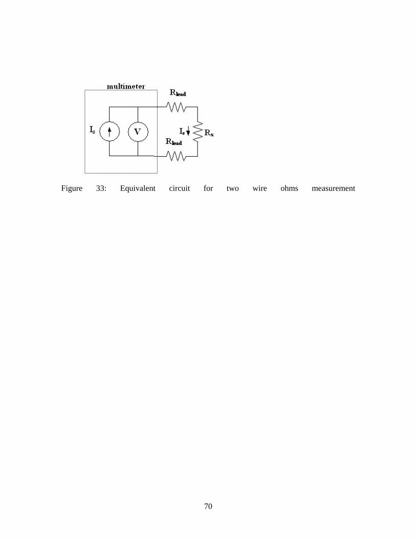
Figure 33: Equivalent circuit for two wire ohms measurement

70

The four wire method

The four-wire method is to be preferred when measuring small resistances since this

method eliminates the lead resistances that can be a problem with the conventional two-

wire method. In figure 34 an equivalent four-wire measurement can be seen. Sense leads

are connected over the unknown resistance to the voltage-meter. A current I is generated

by the current source and drawn through R as well as the two lead resistances R . The

current that flows through the resistances R can be negliged since they often are

several M Ω or as high as 10G. Also the fact that the voltage measured by the meter will

be identical to the voltage developed across the unknown resistance.

s

x lead

sense

Figure 34: Equivalent circuit for four wire ohms measurement

Measurement error and applications When measuring very low resistances (<1 Ω ) even the quality of the cables can interfere

with the result. High quality cables may have resistances in the order of 0,01 Ω . The

measurement error can be calculated as follows

71

Rmeas =Rx + 2Rlead

Rx = Rmeas – 2Rlead

|Error|% = (2Rlead/Rx) * 100

Rmeas/Rx = 1 + (2Rlead/Rx)

The accuracy needed for is often determined by the application, but as a rule of thumb the

two-wire measurement method should only be used when the unknown resistance is

much larger than the lead resistance. Using the four-wire method eliminates the

percentage of measurement error zero of the lead resistances. This type of measurement

can be highly recommended when, for example, measuring ground planes on PCBs.

High resistance measurements

Also when measuring high resistances the two-wire method can be inadequate. If the

unknown resistance under test is a large percentage of the meter’s input resistor

measurement loading errors can be introduced. The measurement error comes from the

internal resistor and the fault arises because of the parallel-connected resistance of the

ohmmeter and the resistance under test. The parallel resistance and the error percentage

can be computed as follows:

Rtotal = (RmRx)/(Rm+Rx)

|Error|% = Rx/(Rx+Rm) * 100

As an example if a resistance with the given resistance Rx of 10k Ω is to be measured and

the ohmmeters internal resistance is 10M Ω the equivalent resistor is 0,999M Ω the

loading error can be computed to 0,1%. If instead R is 10Mx Ω , the equivalent resistance

is 5M Ω and the error is 50%. Also corroded connectors can be a problem when

measuring resistances can be assumed to contribute with as much as 0,1 % error.

Power line noise voltages

72

Power line noise present in dc signals on the input can be eliminated by using analogue to

digital converters, standard on all digital multi meters today. This method reduces

spurious noise to approximately zero, since it averages and integrates the signal over a

fixed period of time. Integration times can be set to a fixed number of whole power line

cycles so that spurious noise and their harmonics are averaged out.

Offset error reduction

Modern advanced multi meters offer features that make it possible to eliminate offset

errors associated with two- and four-wire measurements. With the test leads shorted

together the resistance value of the leads can be stored in the memory and then

automatically subtracted from the measurement. However the two-wire method is not as

accurate as the four wire-measurement method since although the leads have been

shorted together the result will not be the same due to different surface contact resistance.

Offset compensation is another method for improving measurement accuracy. Here the

multi meter measures the external offset voltage without the external current source

connected and then subtracts the offset of the following reading. In this way only the true

induced voltage value is reported. This error correction method can be used with both

two- and four-wire measurements to correct for any thermally induced dc voltages that

cause problems in resistance measurements.

73

Appendix C The following code where used to determine a system optimal PMSM. clear all clf rso = [0.05:0.005:0.25]; ls = [0.01:0.005:0.2]; Bgm1_peak = 1; rho_cu = 1.67e-8; Px = 5000; ksf=0.5; Sigma = 1.6; wnom = 1200/60*2*pi; % 1200 rpm Tnom = 10000/wnom; for i=1:length(rso) for j=1:length(ls) rsi=[0.5*rso(i):0.002*rso(i):0.8*rso(i)]; clear Ttemp tcb dw de Ks1_peak Inertia_temp Mass_temp p for k=1:length(rsi); p(k) = round((2*pi*rsi(k))/((rso(i)-rsi(k))/1.4)/2)*2;

tcb(k) = 2*pi*rsi(k)/p(k)*(Bgm1_peak*2/pi)/2/1.4; % thickness core back, assuming 1.4 times higher flux density than in the air gap

A_ext(i,j) = 2*pi*rso(i)*ls(j); % External cooling area (radial surface) Pcool(i,j) = A_ext(i,j)*Px; % Cooling power, assuming a certian (Px) cooling power density [W/m2]

Pcu(i,j) = Pcool(i,j)/2; % Copper losses, assuming then to be half the total losses (rough) de(k) = (rso(i) - rsi(k) - tcb(k))/2; % Equivalent depth of winding area, assuming half slot and half tooth Ks1_peak(k) = sqrt((Pcu(i,j)*de(k)*ksf)/(rho_cu*pi*rsi(k)*(ls(j)+Sigma*2*pi*rsi(k)/p(k)))); % Peak of linear current density [A/m peripherial length]

% T = F/A * A * r Ttemp(k) = Bgm1_peak*Ks1_peak(k)/2*2*pi*rsi(k)*ls(j)*rsi(k); % Torque with this combination of inner and outer stator radius and length etc

Inertia_temp(k) = 7900*pi*(rsi(k))^2*ls(j)*(rsi(k)^2); % Inertia assuming an average rotor weigth of 7900 kg/m3

Mass_temp(k) = 7900*pi*rso(i)^2*ls(j); end [value,index] = max(Ttemp); % Find the best (=strongest) rotor radius Tmax(i,j) = Ttemp(index); % Save the best torque ... Inertia(i,j) = Inertia_temp(index); % ... and inertia Mass(i,j) = Mass_temp(index); Maxp(i,j) = p(index); end end

74

C = contourc(ls,rso,Tmax,[Tnom Tnom]) NomInertia = Interp2(ls,rso,Inertia,C(1,2:1+C(2,1)),C(2,2:1+C(2,1))) NomMass = Interp2(ls,rso,Mass,C(1,2:1+C(2,1)),C(2,2:1+C(2,1))) figure(2) clf subplot(3,1,1) plot(C(1,2:1+C(2,1)),NomInertia) title('Inertia [kgm^2/m] = f(motor length)') grid subplot(3,1,2) plot(C(1,2:1+C(2,1)),C(2,2:1+C(2,1))) title('Motor radius [m] = f(motor length)') grid subplot(3,1,3) plot(C(1,2:1+C(2,1)),NomMass) title('Motor mass [kg] = f(motor length)') grid figure(1) clf % Pcu = rho_cu*(ls+Sigma*2*pi*rsi/p)/(2*pi*rsi*de*ksf)*(Ks1/sqrt(2)*2*pi*rsi)^2 % Pcu = rho_cu*(ls+Sigma*2*pi*rsi/p)*2*pi*rsi*(de*ksf)*(Ks1/sqrt(2)/(de*ksf))^2 % Pcu = rho_cu*(ls+Sigma*2*pi*rsi/p)*2*pi*rsi/(de*ksf)*Ks1^2/2 % Ks1 = sqrt(2*Pcu*(de*ksf)/(rho_cu*(ls+Sigma*2*pi*ris/p)*2*pi*rsi)) % % T = Bgm1*Ks1/2*2*pi*rsi^2*ls = Bgm1*Ks1*pi*rsi^2*ls = % = Bgm1*sqrt(2*Pcu*(de*ksf)/(rho_cu*(ls+Sigma*2*pi*ris/p)*2*pi*rsi))*pi*rsi^2*ls subplot(2,3,1) contour(ls,rso,Tmax,[1 1]*Tnom) hold on contour(ls,rso,Tmax./Inertia) title('Tnom & T/J isobar') axis([0 max(ls) 0 max(rso)]) subplot(2,3,2) mesh(ls,rso,Inertia) title('Inertia') subplot(2,3,3) mesh(ls,rso,Tmax./Inertia) title('T/J') subplot(2,3,4) contour(ls,rso,Tmax,[1 1]*Tnom) hold on contour(ls,rso,Tmax./Mass) title('Tnom & T/Mass isobar') subplot(2,3,5) mesh(ls,rso,Mass) title('Mass') subplot(2,3,6) mesh(ls,rso,Tmax./Mass) title('T/Mass')

75

electrically synchronised gear shifting industrial ... document/5218_full... · dept. of industrial...

Documents