electric welding arc modeling with the solver...
TRANSCRIPT
Electric welding arc modeling with the solver OpenFOAM
- A comparison of different electromagnetic models -
Isabelle Choquet1, Alireza Javidi Shirvan1, Håkan Nilsson2
1University West, Department of Engineering Science, Trollhättan, Sweden,2Chalmers University of Technology, Department of Applied Mechanics, Gothenburg, Sweden
ABSTRACT
This study focuses on the modeling of a plasma arc heat source in the context ofelectric arc welding. The model was implemented in the open source CFD softwareOpenFOAM-1.6.x, coupling thermal fluid mechanics in three dimensions with electro-magnetics. Four different approaches were considered for modeling the electromag-netic fields: i) the three-dimensional approach, ii) the two-dimensional axi-symmetricapproach, iii) the electric potential formulation, and iv) the magnetic field formulationas described by Ramírez et al. [1]. The underlying assumptions and the differencesbetween these models are described in detail. Models i) to iii) reduce to the same quasione-dimensional limit for an axi-symmetric configuration with negligible radial currentdensity, contrary to model iv). Models ii) to iv) do not represent the same physics whenthe radial current density is significant, such as or an electrode with a conical tip. Mod-els i) to iii) were retained for the numerical simulations. The corresponding results werevalidated against the analytic solution of an infinite electric rod. Perfect agreement wasobtained for all the models tested. The results from the coupled solver (thermal fluidmechanics coupled with electromagnetics) were compared with experimental measure-ments for Gas Tungsten Arc Welding (GTAW). The shielding gas was argon, the arc wasshort (2mm), the electrode tip was conical, and the configuration was axi-symmetric.The boundary conditions were specified at the anode and cathode surfaces. Modelsi) and ii) lead to the same results, but not the model iii). Model iii) neglects the radialcurrent density component, resulting in a poor estimation of the magnetic field, and inturn of the arc fluid velocity. The limitations of the coupled solver were investigatedchanging the gas composition, and using different boundary conditions. The boundaryconditions, difficult to measure and to estimate a priori, significantly affect the simulationresults.
Keywords: electric arc welding, thermal plasma, short arc, electromagnetic model,electric potential formulation, magnetic field formulation, GTAW.
1 INTRODUCTION
The first man made electric arc was produced in 1800by Sir Humphry Davy using carbon electrodes. Elec-tric arc welding as a method of assembling metalparts through fusion was however initiated much later,
at the end of the 19’s century, when C.L. Coffin in-troduced the metal electrode and the metal transferacross an arc. Thanks to intense developments in theearly 1900’s, such as the first coated electrode devel-oped by A.P. Strohmenger and O. Kjellberg, electricarc welding started being utilized in production in the
1
2 Doc. 212-1189-11
1920’s, and then in large scale production from the1930’s.
This manufacturing process, although used sincemany decades, is still under intensive development,in order to further improve different aspects such asprocess productivity, process control, and weld qual-ity. Such improvements are beneficial both from eco-nomical and environmental sustainability.
Electric arc welding is interdisciplinary in nature, andcomplex to master as it involves very large tempera-ture gradients, and a number of parameters that dointeract in a non-linear way. Its investigation waslong based on experimental studies. Today, thanksto recent and significant progress done in the fieldof welding simulation, experiments can be comple-mented with numerical modeling to reach a deeperprocess understanding. As an illustration, the changein microstructure can be simulated for a given thermalhistory within the heat affected zone of the base metal,as shown in [2]. Numerical calculations of the resid-ual stresses, to investigate fatigue and distortion, cannow be coupled with the weld pool as in [3], calibratingfunctional approximations of volume and surface heatflux transferred from the electric arc.
Electric arcs used in welding are generally couplingan electric discharge between an anode and a cath-ode, with a shielding gas flow. The main goal is toform a shielding gas flow with a temperature largeenough to melt the materials to be welded, i.e. a ther-mal plasma flow. The numerical modeling of thermalplasma flow is thus a key element for characterizingthe thermal history of an electric arc welding process.It determines the thermal energy provided to the par-ent metal, its spatial distribution, and also the pressureforce applied by the arc on the weld pool.
A thermal plasma is basically modeled coupling ther-mal fluid mechanics (governing mass, momentum andenergy or enthalpy) with electromagnetics (govern-ing the electric field, the magnetic field, and the cur-rent density). Different thermal plasma models canbe found in the literature in the context of electricarc simulation. The first model coupling thermal fluidmechanics and electromagnetics to simulate an axi-symmetric high-intensity free burning arc was devel-oped by Hsu et al. in 1983, and applied to a 10 mmlong arc [4]. Since then many developments havebeen done to address in more detail various aspectsof the electric arc heat source. Within the frame of axi-
symmetric configurations, Tanaka et al. accounted forchemical non-equilibrium [5]. Yamamoto et al. investi-gated the influence of metal vapor on the properties ofa plasma arc [6]. Wendelstorf coupled arc, anode andcathode including the plasma sheath [7]. Tanaka et al.and Hu et al. coupled arc and weld pool acounting formelting [8], [9]. Some of these models have also beenextended to three space-dimensions by Xu et al. forinstance [10]. These studies are based on the samethermal fluid model (up to the space dimension) for de-scribing the core of the plasma arc. However, variousmodels are used for determining the electromagneticfields. Among them are the three-dimensional formu-lation with magnetic potential, Gonzales et al. [11], orwith magnetic field, Xu et al. [10]. In the context of axi-symmetric applications few authors use the magneticfield formulation introduced by McKelliget and Szekely[14]. Few authors, such as Lago et al. [12], Bini etal. [13], use instead a two-dimensional axi-symmetricmodel (combining the magnetic field formulation with aPoisson equation for governing the electric potential).The electric potential formulation introduced by Hsu etal. [4] is retained by many authors. The electric po-tential formulation and the magnetic field formulation,developed for two-dimensional axi-symmetric configu-rations, were initially applied to rather long arcs with-out accounting for the geometry of the electrode tip.These formulations have been compared by Ramírezet al. [1] for arc lengths of 6.3 and 10 mm. It is oftenconsidered that these formulations do represent thesame physics. When tested numerically, it is howeverobserved that they do lead to results presenting somedifferences. These differences are usually consideredto be due to mathematical and numerical issues, asunderlined by Ramirez et al., [1].
The aim of the present study is to develop a simu-lation tool for thermal plasma arc applied to electricarc welding, and thus to short arcs. The implemen-tation was done in the open source CFD softwareOpenFOAM-1.6.x (www.openfoam.com), consideringthree space dimensions. OpenFOAM was distributedas OpenSource in 2004. This simulation software isa C++ library of object-oriented classes that can beused for implementing solvers for continuum mechan-ics. It includes a number of solvers for different con-tinuum mechanical problems. Due to the availabilityof the source code, its libraries can be used to imple-ment new solvers for other applications. The current
Doc. 212-1189-11 3
implementation is based on the buoyantSimpleFoamsolver, which is a steady-state solver for buoyant, tur-bulent flow of compressible fluids. The partial differ-ential equations of this solver are discretized using thefinite volume method.The thermal plasma simulation model implemented inteh present work is described in section 2. It couplesa system of thermal Navier-Stokes equations in threespace-dimensions (section 2.1) with a simplified sys-tem of Maxwell equations (section 2.2). Different sim-plifications were considered for modeling the electro-magnetic fields:
i) the three-dimensional approach,
ii) the two-dimensional axi-symmetric approach,
iii) the quasi one-dimensional approach,
iv) the electric potential formulation, and
v) the magnetic field formulation.
The underlying assumptions and the differences be-tween these models are detailed in section 2.2.
Models i), ii) and iv) were retained for doing numeri-cal tests. The electromagnetic part of the solver wastested against the analytic solution of an infinite elec-tric rod. The test case and the results are presentedin section 3.1.The coupled solver was tested against experimentalmeasurements for Gas Tungsten Arc Welding (GTAW)done by Haddad and Farmer [15]. That case was alsoused by Tsai and Sindo Kou [16] for modeling and sim-ulating welding arcs produced by sharpened and flatelectrodes. The shielding of the test case gas is ar-gon, the experimental configuration is axi-symmetric,and the arc length (2 mm) is not long compared to theelectrode tip radius (0.5 mm). The anode and cath-ode were treated as boundary conditions in the simu-lations, accounting for the geometry of the electrodetip. This second test case, and the related simulationresults, are presented in section 3.2. For each testcase the approaches i), ii) and iv) were used for calcu-lating the magnetic field, and their validity discussed.The limitations of the coupled solver were also investi-gated changing the gas composition, and testing vari-ous boundary conditions on the anode and cathode toevaluate their influence on the plasma arc. The cor-responding simulation results are presented and dis-cussed in sections 3.3 and 3.4. The main results andconclusions are summarized in section 4.
2 MODEL
The model described in the present work was retainedas first step in the development of a simulation toolfor thermal plasma arc applied to electric arc weld-ing. The implementation was done in the continuationof the work done by Sass-Tisovskaya [17]. The im-plementation was done in the open source CFD soft-ware OpenFOAM-1.6.x (www.openfoam.com), cou-pling thermal fluid mechanics with electromagnetics.The fluid and electromagnetic models are tightly cou-pled. The Lorentz force, or magnetic pinch force, re-sulting from the induced magnetic field indeed actsas the main cause of plasma flow acceleration. TheJoule heating due to the electric field is the largestheat source governing the plasma energy (and thustemperature). On the other hand the system of equa-tions governing electromagnetics is temperature de-pendent, via the electric conductivity. The main detailsof the implemented thermal fluid and electromagneticmodels are described in the following sections.
2.1 Thermal fluid model
The thermal fluid part of the model was derived byChoquet and Lucquin-Desreux [18] from a system ofBoltzmann type transport equations using kinetic the-ory. A viscous hydrodynamic/diffusion limit was ob-tained in two stages doing a Hilbert expansion andusing the Chapman-Enskog method. The resultantviscous fluid model is characterized by two temper-atures, and non equilibrium ionization. It applies tothe arc plasma core and the ionization zone of the arcplasma sheath. The model implemented here is a sim-plified version of that model neglecting the arc plasmasheath. The thermal fluid component of the model ap-plies to a Newtonian and thermally expansible fluid,assuming:
- a one-fluid model,
- in local thermal equilibrium,
- mechanically incompressible,because of the small Mach number, and
- a steady-state and laminar flow.
The model is thus suited to the plasma core. In thisframework the continuity equation is written as
O·[ρ(T ) ~u
]= 0 , (1)
4 Doc. 212-1189-11
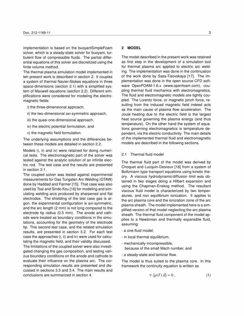
where ρ denotes the fluid density, ~u the fluid velocity,and O· the divergence operator. The density ρ = ρ(T )depends here on the temperature T , as illustrated forargon plasma in Fig. 1.
Figure 1: Argon plasma density as a function oftemperature.
The momentum conservation equation is expressedas
O·[ρ(T ) ~u ⊗ ~u
]− ~u O·
[ρ(T ) ~u
]−O·
[µ(T )
(O~u + (O~u)T
)− 2
3 µ(T ) (O·~u) I]
= −OP + ~J × ~B ,
(2)
where µ the viscosity, I is the identity tensor, P thepressure, ~B the magnetic flux density (simply calledmagnetic field in the sequel), ~J the current density, Odenotes the gradient operator, ⊗ and × the tensorialand vectorial product, respectively. The last term onthe right hand side of Eq. (2) is the Lorentz force.The enthalpy conservation equation is
O·[ρ(T )~u h
]− h O ·
[ρ(T ) ~u
]− O·
[α(T ) Oh
]= O· (~u P) − P O·~u + ~J· ~E
−Qrad + O·[ 5 kB ~J2 e Cp(T )
h],
(3)
where h is the specific enthalpy, α is the thermal dif-fusivity, ~E the electric field, Qrad the radiation heatloss [19], kB the Boltzmann constant, e the elementarycharge, and Cp the specific heat at constant pressure.
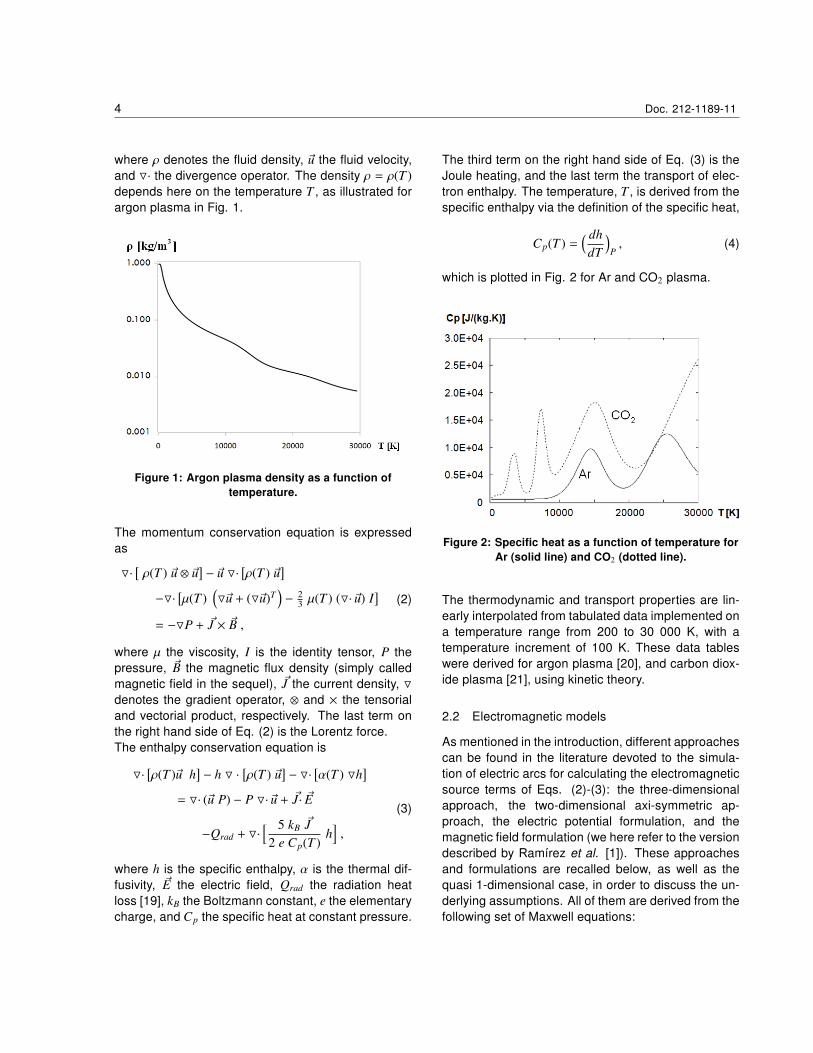
The third term on the right hand side of Eq. (3) is theJoule heating, and the last term the transport of elec-tron enthalpy. The temperature, T , is derived from thespecific enthalpy via the definition of the specific heat,
Cp(T ) =( dhdT
)P, (4)
which is plotted in Fig. 2 for Ar and CO2 plasma.
Figure 2: Specific heat as a function of temperature forAr (solid line) and CO2 (dotted line).
The thermodynamic and transport properties are lin-early interpolated from tabulated data implemented ona temperature range from 200 to 30 000 K, with atemperature increment of 100 K. These data tableswere derived for argon plasma [20], and carbon diox-ide plasma [21], using kinetic theory.
2.2 Electromagnetic models
As mentioned in the introduction, different approachescan be found in the literature devoted to the simula-tion of electric arcs for calculating the electromagneticsource terms of Eqs. (2)-(3): the three-dimensionalapproach, the two-dimensional axi-symmetric ap-proach, the electric potential formulation, and themagnetic field formulation (we here refer to the versiondescribed by Ramírez et al. [1]). These approachesand formulations are recalled below, as well as thequasi 1-dimensional case, in order to discuss the un-derlying assumptions. All of them are derived from thefollowing set of Maxwell equations:
Doc. 212-1189-11 5
Gauss’ law for magnetism
O· ~B = 0 , (5)
Gauss’ law
O· ~E = ε−1o qtot , (6)
Faraday’s law
∂~B∂t
= −O × ~E , (7)
and, Ampère’s law
εo µo∂~E∂t
= O × ~B − µo ~J , (8)
where qtot is the total electric charge per unit volume,εo the permittivity of vacuum, µo the permeability ofvacuum, and O× denotes the rotational operator.The Maxwell equations are supplemented by theequation governing charge conservation
∂qtot
∂t+ O· ~J = 0 , (9)
and the generalized Ohm law
~J = ~Jdrift + ~Jind + ~JHall + ~Jdiff + ~Jther , (10)
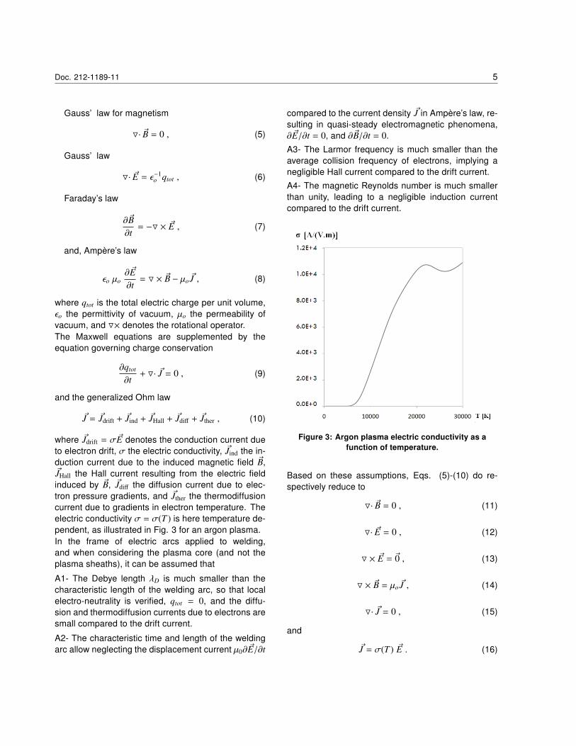
where ~Jdrift = σ~E denotes the conduction current dueto electron drift, σ the electric conductivity, ~Jind the in-duction current due to the induced magnetic field ~B,~JHall the Hall current resulting from the electric fieldinduced by ~B, ~Jdiff the diffusion current due to elec-tron pressure gradients, and ~Jther the thermodiffusioncurrent due to gradients in electron temperature. Theelectric conductivity σ = σ(T ) is here temperature de-pendent, as illustrated in Fig. 3 for an argon plasma.In the frame of electric arcs applied to welding,and when considering the plasma core (and not theplasma sheaths), it can be assumed that
A1- The Debye length λD is much smaller than thecharacteristic length of the welding arc, so that localelectro-neutrality is verified, qtot = 0, and the diffu-sion and thermodiffusion currents due to electrons aresmall compared to the drift current.
A2- The characteristic time and length of the weldingarc allow neglecting the displacement current µ0∂~E/∂t
compared to the current density ~J in Ampère’s law, re-sulting in quasi-steady electromagnetic phenomena,∂~E/∂t = 0, and ∂~B/∂t = 0.
A3- The Larmor frequency is much smaller than theaverage collision frequency of electrons, implying anegligible Hall current compared to the drift current.
A4- The magnetic Reynolds number is much smallerthan unity, leading to a negligible induction currentcompared to the drift current.
Figure 3: Argon plasma electric conductivity as afunction of temperature.
Based on these assumptions, Eqs. (5)-(10) do re-spectively reduce to
O· ~B = 0 , (11)
O· ~E = 0 , (12)
O × ~E = ~0 , (13)
O × ~B = µo ~J , (14)
O· ~J = 0 , (15)
and
~J = σ(T ) ~E . (16)
6 Doc. 212-1189-11
The set of equations (11)-(16) are usually combinedin the following more convenient form. As the elec-tric field ~E is irrotational (from Eq. (13)), as the mag-netic field ~B is of constant zero divergence (from Eq.(11)), and electromagnetic phenomena can be as-sumed quasi-steady (assumption A2), there exist ascalar electric potential V and a vector magnetic po-tential ~A defined up to a constant such that,
~E = −OV , (17)
and
~B = O × ~A . (18)
Using these properties, Eqs. (15) and (16) lead to thePoisson scalar equation governing the electric poten-tial
O· [σ(T ) OV] = 0 . (19)
The remaining equation (14) leads to the vector equa-tion governing the magnetic potential,
O × O × ~A = O·(O~A
)− 4~A = µo ~J , (20)
where 4 denotes the Laplace operator.An additional condition then needs to be imposed inorder to uniquely define ~A and V. This condition isgiven here by the Lorentz gauge, O~A = 0. Then, usingEqs. (16) and (17), the equation governing the mag-netic potential ~A reduces to the Poisson vector equa-tion
4~A = µo σ(T ) OV . (21)
2.2.1 Three-dimensional approach
When considering a three-dimensional approach theelectromagnetic model for a welding arc plasma coreuses Eqs. (19) and (21). The electric field ~E, theelectric current ~J and the magnetic field ~B entering thesource terms of the fluid set of equations (section 2.1)are derived from V and ~A through Eqs. (17), (16), and(18), respectively.It should be noticed that the model used by Xu et al.[10] is the same, although these authors did not intro-duce explicitly the magnetic potential.
2.2.2 Two-dimensional axi-symmetric approach
Here, the particular case of an axi-symmetric con-figuration is considered, such as water cooled cath-ode TIG welding. A cylindrical coordinate system(r, θ, z) is then introduced. Additional simplificationscan now be done thanks to the invariance by rota-tion about the symmetry axis. It results in no gra-dient along the azimuthal direction θ, a current den-sity ~J(r, z) =
(Jr(r, z), 0, Jz(r, z)
)with a constant zero
angular component Jθ = 0, and a magnetic field~B(r, z) = (0, Bθ(r, z), 0) along the azimuthal direction.Then the electromagnetic model of section 2.2.1 sim-plifies to the Poisson equation governing the electricpotential V(r, z)
1r∂
∂r
(r σ(T )
∂V∂r
)+∂
∂z
(σ(T )
∂V∂z
)= 0 , (22)
and two scalar Poisson equations governing the mag-netic potential ~A(r, z) = (Ar(r, z), 0, Az(r, z))
1r∂
∂r
(r∂Ar
∂r
)+∂2Ar
∂z2 −Ar
r2 = µo σ(T )∂V∂r
, (23)
and
1r∂
∂r
(r∂Az
∂r
)+∂2Az
∂z2 = µo σ(T )∂V∂z
. (24)
Using the Lorentz gauge
1r∂(rAr)∂r
+∂Az
∂z= 0 , (25)
and the definition of the magnetic potential, Eq. (18),we can easily see that Eqs. (23)-(24) also write
∂Bθ∂z
= µo σ(T )∂V∂r
= −µo Jr , (26)
and
1r∂(rBθ)∂r
= −µo σ(T )∂V∂z
= µo Jz , (27)
which is the Gauss law in cylindrical coordinates andin the particular case of an axi-symmetric problem.Eqs. (26)-(27) can be condensed into a single re-lation, for which two options are possible. The firstoption leads to a partial differential equation and thesecond to an integral relation defining Bθ. The partialdifferential formulation
∂
∂r
( 1σr
∂(rBθ)∂r
)+∂
∂z
( 1σ
∂Bθ∂z
)= 0 , (28)
Doc. 212-1189-11 7
is easily derived from Eqs. (26)-(27) as ∂2V/(∂r∂z) =
∂2V/(∂z∂r). It should be noticed that Eq. (28) is theinduction diffusion equation involved in the magneticfield formulation.The integral formulation is also derived from Eqs.(26)-(27), using now the fact that ∂2Bθ/(∂r∂z) =
∂2Bθ/(∂z∂r), so that
1r∂Bθ∂z
= µo
(∂Jr
∂r+∂Jz
∂z
), (29)
and thus
Bθ(r, z) − Bθ(r, zo)
= r µo
∫ l=z
l=zo
(∂Jz
∂z+∂Jr
∂r
)(r, l) dl .
(30)
This integral relation defining the azimuthal compo-nent of the magnetic field can be further simplified to
Bθ(r, z) = −µo
∫ l=z
l=zo
Jr(r, l) dl + Bθ(r, zo) , (31)
using the Poission equation (22) and the relations
Jr(r, z) = σ(T ) Er(r, z) = −σ(T )∂V∂r
, (32)
and
Jz(r, z) = σ(T ) Ez(r, z) = −σ(T )∂V∂z
, (33)
resulting from Eqs. (16) and (17).
To summarize, when considering a two-dimensionalaxi-symmetric approach the electromagnetic modelfor a welding arc plasma core is made of three scalarequations or less depending on the formulation re-tained for deriving the magnetic field. These equationsinclude:
- the scalar Poisson equation, Eq. (22), governing theelectric potential V, supplemented by the Eqs. (32)and (33) for deriving the electric field and the currentdensity, and
- either B1, B2 or B3 for deriving the azimuthal com-ponent of the magnetic field:
B1 - The two scalar Poisson equations, Eqs. (23)-(24),governing the non-zero components of the magneticpotential ~A, supplemented by Eq. (18) yielding
Bθ(r, z) =∂Ar
∂z−∂Az
∂r. (34)
B2- The scalar induction diffusion equation, Eq. (28).
B3- The integral relation, Eq. (31).
B1 to B3 are based on the same assumptions. Formu-lation B3 seems to be the simplest one, with only oneintegral relation and no additional partial differentialequation to solve. However it requires setting the ref-erence value for the magnetic field, Bθ(r, zo) at somewell chosen location zo, which is a difficulty. Also, in-tegrating the current along the axial direction may re-quire a careful implementation work when accountingfor electrode tip angle (the cells of the mesh may notbe everywhere aligned along the axial direction). B2may thus be easier to implement if the interior of theanode and cathode is included in the computationaldomain, since then the magnetic field can easily beset on the boundaries of the computational domain.However if, as in the present study, only the surfaceof the anode and cathode is accounted for (as bound-ary of the computational domain), the specification ofthe magnetic field on the boundaries may turn out tobe difficult too. In that case formulation B1 based onthe magnetic potential is indeed more convenient, andthus retained for the simulation tests of section 3. No-tice that formulation B1 was also used by Lago et al.[12] and Bini et al. [13] for instance.
2.2.3 Quasi one-dimensional approach
Here a simpler axi-symmetric case is considered, as-suming in addition a negligible radial current density.The current density vector is thus aligned with the di-rection of the symmetry axis, ~J(r) = (0, 0, Jz(r)), andthe magnetic field is azimuthal with ~B(r) = (0, Bθ(r), 0).The scalar Poisson equation governing the electric po-tential, Eq. (22), now further simplifies to
∂
∂z
(σ(T )
∂V∂z
)= 0 , (35)
with the remaining vector component
Jz = σ(T ) Ez = −σ(T )∂V∂z
. (36)
Eqs. (26)-(27) reduce to
1r∂ (r Bθ)∂r
= µo Jz , (37)
8 Doc. 212-1189-11
so that the magnetic field can be defined by the follow-ing well-known integral relation
Bθ(r) =µo
r
∫ l=r
l=ro
l Jz(l) dl + Bθ(ro) . (38)
The reference value Bθ(ro) can easily be set to zerotaking the symmetry axis as reference location (ro =
0).The electric potential formulation and the magneticfield formulation, which are more commonly used thanthe axi-symmetric approach of section 2.2.2 and thequasi one-dimensional approach of section 2.2.3, arerecalled below. Each of these formulations is a simpli-fied version of the axi-symmetric approach. The sim-plifications have the advantage of further reducing theelectromagnetic model down to a single partial differ-ential equation.
2.2.4 The electric potential formulation
The electric potential formulation, detailed in [4], com-bines two different levels of modeling:
- a two-dimensional axi-symmetric approach for defin-ing the electric potential, Eq. (22), the current densityand the electric field, Eqs. (32)-(33), with
- a quasi one-dimensional approach for defining themagnetic field, Eq. (38).
It should be noticed that in the limit of a negligible ra-dial current density compared to the axial current den-sity, the electric potential formulation reduces to thequasi one-dimensional formulation (section 2.2.3).
The electric potential formulation was initially appliedto long arcs, i.e. arcs with a distance between anodeand cathode rather large compared to the electroderadius. In addition it was applied, such as in the workby Hsu et al. [4] and Ramirez et al. [1], considering thedomain below the electrode and not next to it. Also theboundary conditions set were those of an infinite elec-tric rod. In this framework the radial current densitycomponent is less than the axial current density com-ponent, so that the quasi one-dimensional approachfor the magnetic field is a good approximation.The electric potential formulation is known to be ac-curate for predicting the arc temperature for axi-symmetric configurations [1]. This is indeed due tothe fact that the axi-symmetric formulation (section2.2.2) and the electric potential formulation are based
on the same assumptions for defining the electric po-tential. However, the electric potential formulation isalso known to be less accurate for calculating the arcvelocity [1]. This is due to the simplification done whenevaluating the magnetic field. This lower accuracy,almost negligible for long arcs, is thus expected tobe more significant when two-dimensional effects be-come more important, i.e. for short arcs, and/or whenconsidering the geometry of the electrode tip (such asa tip angle).
2.2.5 The magnetic field formulation
The magnetic field formulation, introduced by McK-elliget and Szekely [14], is derived from the axi-symmetric approach alone. As underlined by Ramirezet al. [1], an advantage of this formulation is to allowderiving the current density from the azimuthal com-ponent of the magnetic field without the need to solvethe electric potential or the electric field. This formula-tion is indeed made of
- the induction diffusion equation, Eq. (28), for definingthe magnetic field, from which the current density isdirectly derived using Eqs. (26)-(27).
Contrary to the electric potential formulation, the mag-netic formulation is known to be accurate for predict-ing the arc velocity, but less accurate for calculatingthe arc temperature since the determination of the ax-ial current density from the azimuthal magnetic field,Eq. (27), introduces a non-physical singularity on thesymmetry axis [1].
It should be noticed that in the limit of a negligible ra-dial current density compared to the axial current den-sity, this formulation does not reduce to the quasi one-dimensional formulation of section 2.2.3. It reducesonly to Eqs. (37) and (38), which are the same. Inthis limit it indeed defines Bθ from Jz , and at thesame time Jz from Bθ. This implies that the quasione-dimensional limit of the magnetic field formula-tion is not closed. Also, as detailed in section 2.2.2,the induction diffusion equation, Eq. (28), is derivedfrom Eqs. (26)-(27), themselves derived from Gauss’law for magnetism and Ampère’s law. The magneticfield formulation is thus a non-closed version of theaxi-symmetric model since it does not account for thecharge conservation equation. On the contrary, theelectric potential formulation is closed, using the quasione-dimensional closure relation, Eq. (38).
Doc. 212-1189-11 9
3 TEST CASES
Two test cases were investigated, see section 3.1and 3.2, to study the influence of the two-dimensionalphenomena in connection with the electromagneticmodel. For this reason, the quasi one-dimensionalapproach of section 2.2.3 was not retained. The elec-tromagnetic models used in these simulation tests arethe remaining closed models:
i) the three-dimensional approach,
ii) the two-dimensional axi-symmetric approachwith the formulation B1, and
iii) the electric potential formulation.
The first test case, an infinite and electrically conduct-ing rod, was retained since it has an analytic solutionallowing testing the electromagnetic models. The sec-ond is the short arc (2 mm) of the water cooled GTAWtest case described by Tsai and Kou [16]. It was in-vestigated experimentally by Haddad and Farmer [15],and used in the literature as reference for testing archeat source simulation models.
3.1 Infinite rod
The magnetic field induced in and around an infiniterod of radius ro with constant electric conductivity, andconstant current density Jz parallel to the rod axis, re-duces to an azimuthal component Bθ. Bθ has the fol-lowing analytic expression:
Bθ(r) =µoJz r
2if r < ro ,
Bθ(r) =µoJz r2
o
2 rif r ≥ ro ,
(39)
where Jz = I/(π ro) denotes the current density alongthe rod axis, and I the current intensity.A long rod of radius ro = 1 mm with the largeand uniform electric conductivity σrod = 2700A/(Vm),surrounded by a poor conducting region of radiusrext = 16 mm, and uniform electric conductivity σsur =
10−5A/(Vm), was simulated. The conductivity σrod
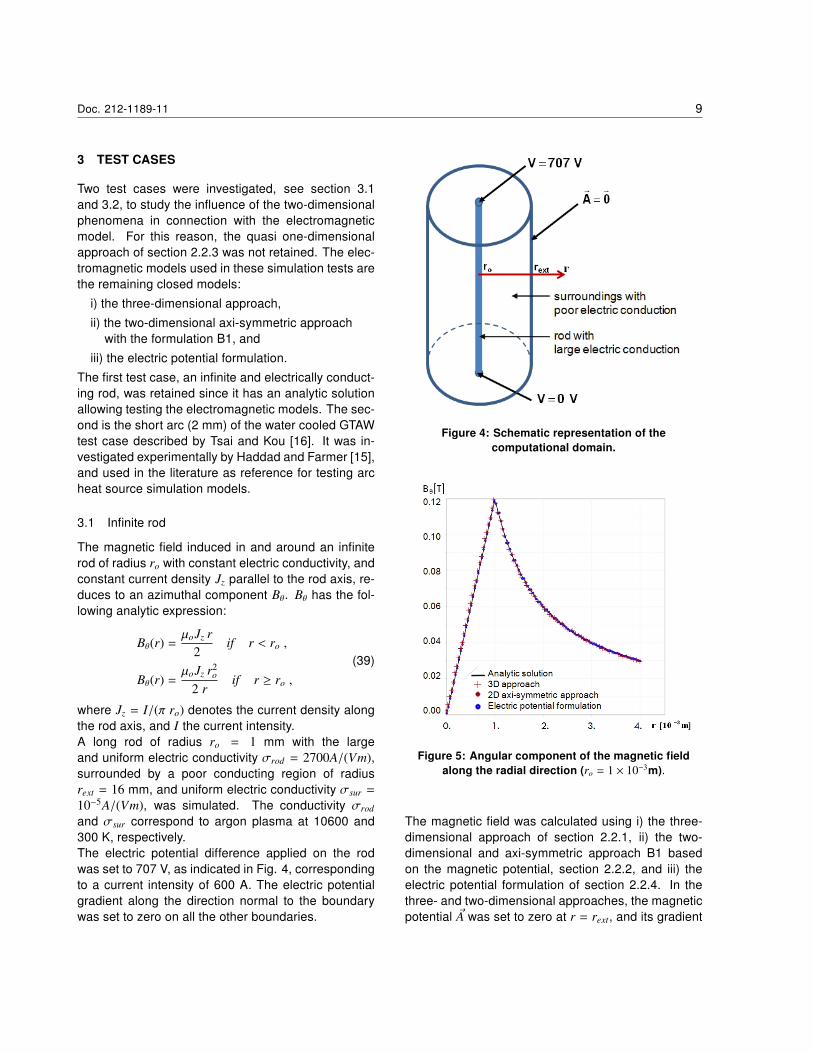
and σsur correspond to argon plasma at 10600 and300 K, respectively.The electric potential difference applied on the rodwas set to 707 V, as indicated in Fig. 4, correspondingto a current intensity of 600 A. The electric potentialgradient along the direction normal to the boundarywas set to zero on all the other boundaries.
Figure 4: Schematic representation of thecomputational domain.
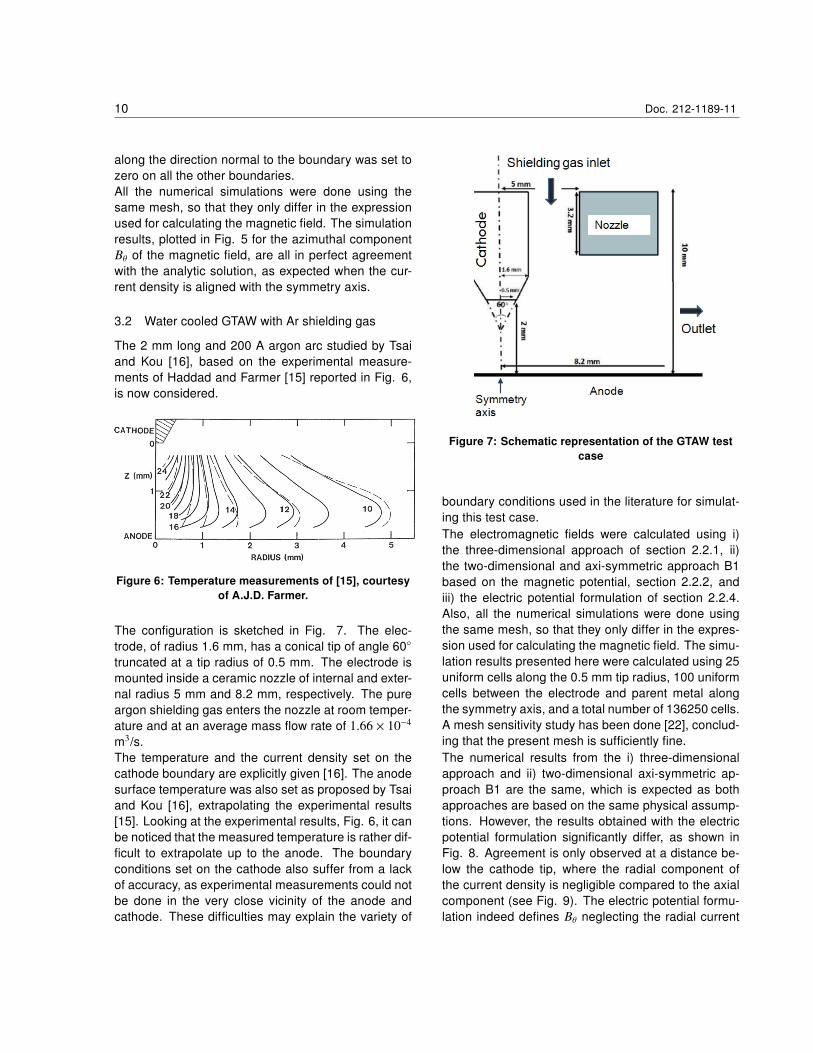
Figure 5: Angular component of the magnetic fieldalong the radial direction (ro = 1 × 10⁻³m).
The magnetic field was calculated using i) the three-dimensional approach of section 2.2.1, ii) the two-dimensional and axi-symmetric approach B1 basedon the magnetic potential, section 2.2.2, and iii) theelectric potential formulation of section 2.2.4. In thethree- and two-dimensional approaches, the magneticpotential ~A was set to zero at r = rext, and its gradient
10 Doc. 212-1189-11
along the direction normal to the boundary was set tozero on all the other boundaries.All the numerical simulations were done using thesame mesh, so that they only differ in the expressionused for calculating the magnetic field. The simulationresults, plotted in Fig. 5 for the azimuthal componentBθ of the magnetic field, are all in perfect agreementwith the analytic solution, as expected when the cur-rent density is aligned with the symmetry axis.
3.2 Water cooled GTAW with Ar shielding gas
The 2 mm long and 200 A argon arc studied by Tsaiand Kou [16], based on the experimental measure-ments of Haddad and Farmer [15] reported in Fig. 6,is now considered.
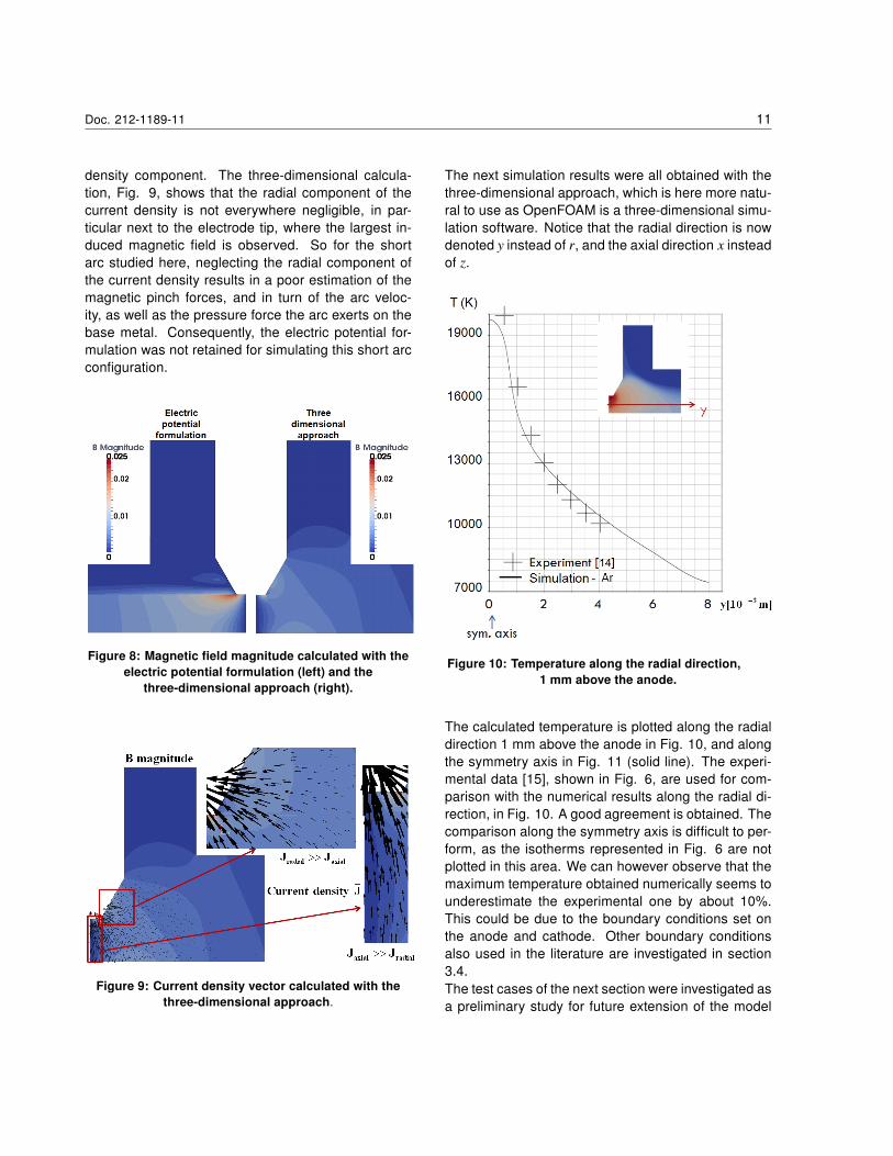
Figure 6: Temperature measurements of [15], courtesyof A.J.D. Farmer.
The configuration is sketched in Fig. 7. The elec-trode, of radius 1.6 mm, has a conical tip of angle 60◦
truncated at a tip radius of 0.5 mm. The electrode ismounted inside a ceramic nozzle of internal and exter-nal radius 5 mm and 8.2 mm, respectively. The pureargon shielding gas enters the nozzle at room temper-ature and at an average mass flow rate of 1.66 × 10⁻⁴
m3/s.The temperature and the current density set on thecathode boundary are explicitly given [16]. The anodesurface temperature was also set as proposed by Tsaiand Kou [16], extrapolating the experimental results[15]. Looking at the experimental results, Fig. 6, it canbe noticed that the measured temperature is rather dif-ficult to extrapolate up to the anode. The boundaryconditions set on the cathode also suffer from a lackof accuracy, as experimental measurements could notbe done in the very close vicinity of the anode andcathode. These difficulties may explain the variety of
Figure 7: Schematic representation of the GTAW testcase
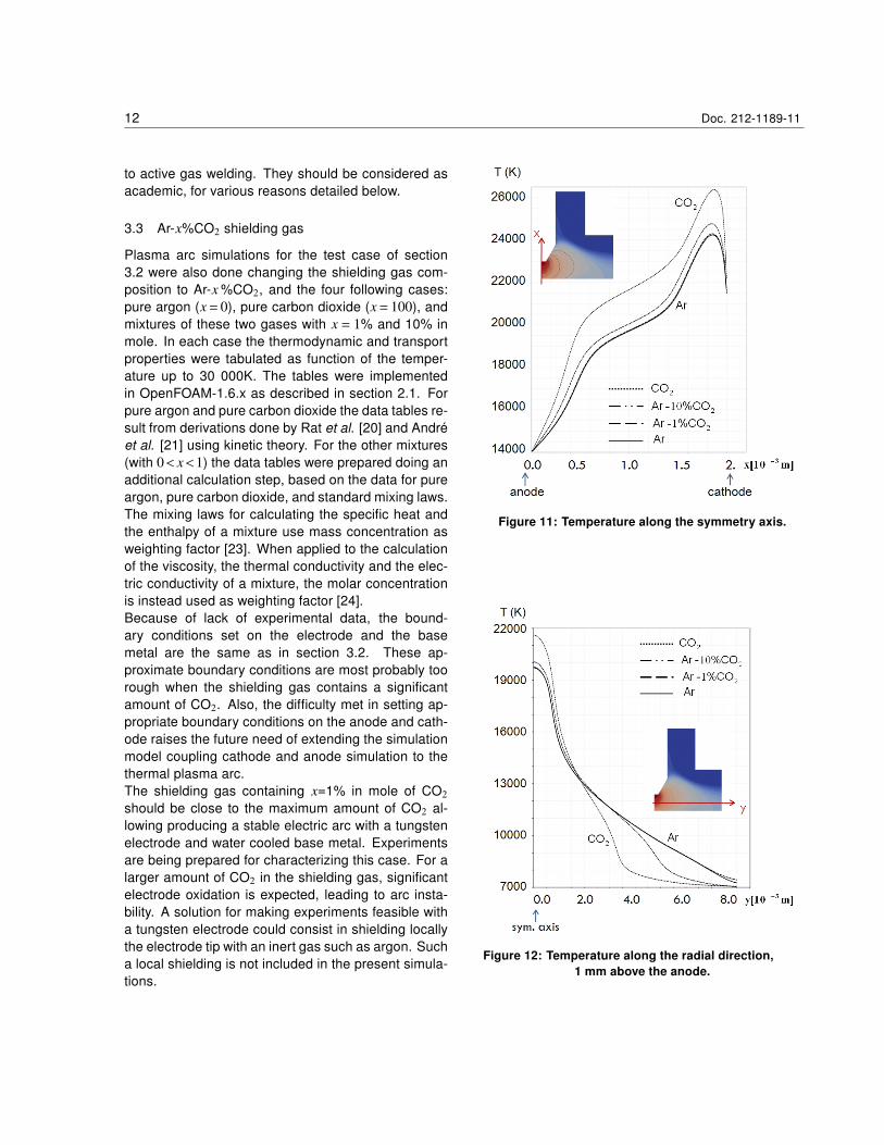
boundary conditions used in the literature for simulat-ing this test case.The electromagnetic fields were calculated using i)the three-dimensional approach of section 2.2.1, ii)the two-dimensional and axi-symmetric approach B1based on the magnetic potential, section 2.2.2, andiii) the electric potential formulation of section 2.2.4.Also, all the numerical simulations were done usingthe same mesh, so that they only differ in the expres-sion used for calculating the magnetic field. The simu-lation results presented here were calculated using 25uniform cells along the 0.5 mm tip radius, 100 uniformcells between the electrode and parent metal alongthe symmetry axis, and a total number of 136250 cells.A mesh sensitivity study has been done [22], conclud-ing that the present mesh is sufficiently fine.The numerical results from the i) three-dimensionalapproach and ii) two-dimensional axi-symmetric ap-proach B1 are the same, which is expected as bothapproaches are based on the same physical assump-tions. However, the results obtained with the electricpotential formulation significantly differ, as shown inFig. 8. Agreement is only observed at a distance be-low the cathode tip, where the radial component ofthe current density is negligible compared to the axialcomponent (see Fig. 9). The electric potential formu-lation indeed defines Bθ neglecting the radial current
Doc. 212-1189-11 11
density component. The three-dimensional calcula-tion, Fig. 9, shows that the radial component of thecurrent density is not everywhere negligible, in par-ticular next to the electrode tip, where the largest in-duced magnetic field is observed. So for the shortarc studied here, neglecting the radial component ofthe current density results in a poor estimation of themagnetic pinch forces, and in turn of the arc veloc-ity, as well as the pressure force the arc exerts on thebase metal. Consequently, the electric potential for-mulation was not retained for simulating this short arcconfiguration.
Figure 8: Magnetic field magnitude calculated with theelectric potential formulation (left) and the
three-dimensional approach (right).
Figure 9: Current density vector calculated with thethree-dimensional approach.
The next simulation results were all obtained with thethree-dimensional approach, which is here more natu-ral to use as OpenFOAM is a three-dimensional simu-lation software. Notice that the radial direction is nowdenoted y instead of r, and the axial direction x insteadof z.
Figure 10: Temperature along the radial direction,1 mm above the anode.
The calculated temperature is plotted along the radialdirection 1 mm above the anode in Fig. 10, and alongthe symmetry axis in Fig. 11 (solid line). The experi-mental data [15], shown in Fig. 6, are used for com-parison with the numerical results along the radial di-rection, in Fig. 10. A good agreement is obtained. Thecomparison along the symmetry axis is difficult to per-form, as the isotherms represented in Fig. 6 are notplotted in this area. We can however observe that themaximum temperature obtained numerically seems tounderestimate the experimental one by about 10%.This could be due to the boundary conditions set onthe anode and cathode. Other boundary conditionsalso used in the literature are investigated in section3.4.The test cases of the next section were investigated asa preliminary study for future extension of the model
12 Doc. 212-1189-11
to active gas welding. They should be considered asacademic, for various reasons detailed below.
3.3 Ar-x%CO2 shielding gas
Plasma arc simulations for the test case of section3.2 were also done changing the shielding gas com-position to Ar-x %CO2, and the four following cases:pure argon (x = 0), pure carbon dioxide (x = 100), andmixtures of these two gases with x = 1% and 10% inmole. In each case the thermodynamic and transportproperties were tabulated as function of the temper-ature up to 30 000K. The tables were implementedin OpenFOAM-1.6.x as described in section 2.1. Forpure argon and pure carbon dioxide the data tables re-sult from derivations done by Rat et al. [20] and Andréet al. [21] using kinetic theory. For the other mixtures(with 0< x<1) the data tables were prepared doing anadditional calculation step, based on the data for pureargon, pure carbon dioxide, and standard mixing laws.The mixing laws for calculating the specific heat andthe enthalpy of a mixture use mass concentration asweighting factor [23]. When applied to the calculationof the viscosity, the thermal conductivity and the elec-tric conductivity of a mixture, the molar concentrationis instead used as weighting factor [24].Because of lack of experimental data, the bound-ary conditions set on the electrode and the basemetal are the same as in section 3.2. These ap-proximate boundary conditions are most probably toorough when the shielding gas contains a significantamount of CO2. Also, the difficulty met in setting ap-propriate boundary conditions on the anode and cath-ode raises the future need of extending the simulationmodel coupling cathode and anode simulation to thethermal plasma arc.The shielding gas containing x=1% in mole of CO2should be close to the maximum amount of CO2 al-lowing producing a stable electric arc with a tungstenelectrode and water cooled base metal. Experimentsare being prepared for characterizing this case. For alarger amount of CO2 in the shielding gas, significantelectrode oxidation is expected, leading to arc insta-bility. A solution for making experiments feasible witha tungsten electrode could consist in shielding locallythe electrode tip with an inert gas such as argon. Sucha local shielding is not included in the present simula-tions.
Figure 11: Temperature along the symmetry axis.
Figure 12: Temperature along the radial direction,1 mm above the anode.
Doc. 212-1189-11 13
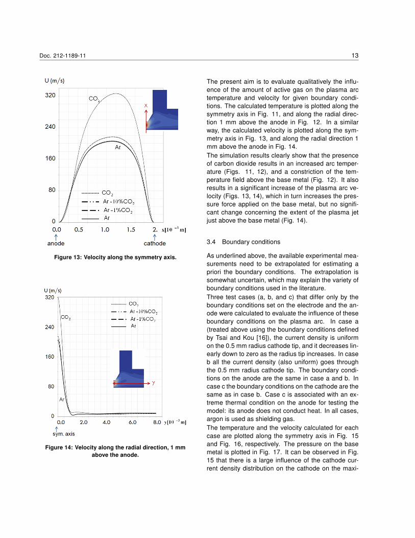
Figure 13: Velocity along the symmetry axis.
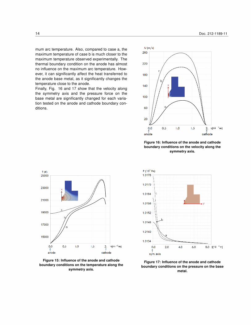
Figure 14: Velocity along the radial direction, 1 mmabove the anode.
The present aim is to evaluate qualitatively the influ-ence of the amount of active gas on the plasma arctemperature and velocity for given boundary condi-tions. The calculated temperature is plotted along thesymmetry axis in Fig. 11, and along the radial direc-tion 1 mm above the anode in Fig. 12. In a similarway, the calculated velocity is plotted along the sym-metry axis in Fig. 13, and along the radial direction 1mm above the anode in Fig. 14.The simulation results clearly show that the presenceof carbon dioxide results in an increased arc temper-ature (Figs. 11, 12), and a constriction of the tem-perature field above the base metal (Fig. 12). It alsoresults in a significant increase of the plasma arc ve-locity (Figs. 13, 14), which in turn increases the pres-sure force applied on the base metal, but no signifi-cant change concerning the extent of the plasma jetjust above the base metal (Fig. 14).
3.4 Boundary conditions
As underlined above, the available experimental mea-surements need to be extrapolated for estimating apriori the boundary conditions. The extrapolation issomewhat uncertain, which may explain the variety ofboundary conditions used in the literature.Three test cases (a, b, and c) that differ only by theboundary conditions set on the electrode and the an-ode were calculated to evaluate the influence of theseboundary conditions on the plasma arc. In case a(treated above using the boundary conditions definedby Tsai and Kou [16]), the current density is uniformon the 0.5 mm radius cathode tip, and it decreases lin-early down to zero as the radius tip increases. In caseb all the current density (also uniform) goes throughthe 0.5 mm radius cathode tip. The boundary condi-tions on the anode are the same in case a and b. Incase c the boundary conditions on the cathode are thesame as in case b. Case c is associated with an ex-treme thermal condition on the anode for testing themodel: its anode does not conduct heat. In all cases,argon is used as shielding gas.The temperature and the velocity calculated for eachcase are plotted along the symmetry axis in Fig. 15and Fig. 16, respectively. The pressure on the basemetal is plotted in Fig. 17. It can be observed in Fig.15 that there is a large influence of the cathode cur-rent density distribution on the cathode on the maxi-
14 Doc. 212-1189-11
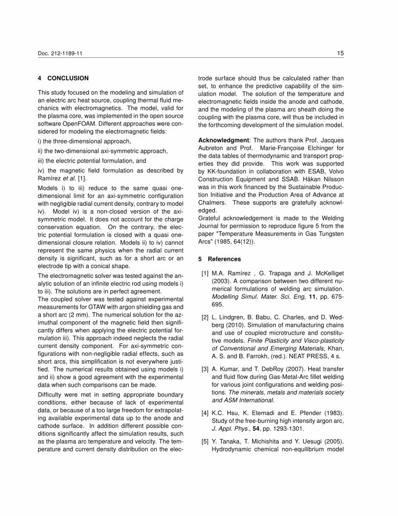
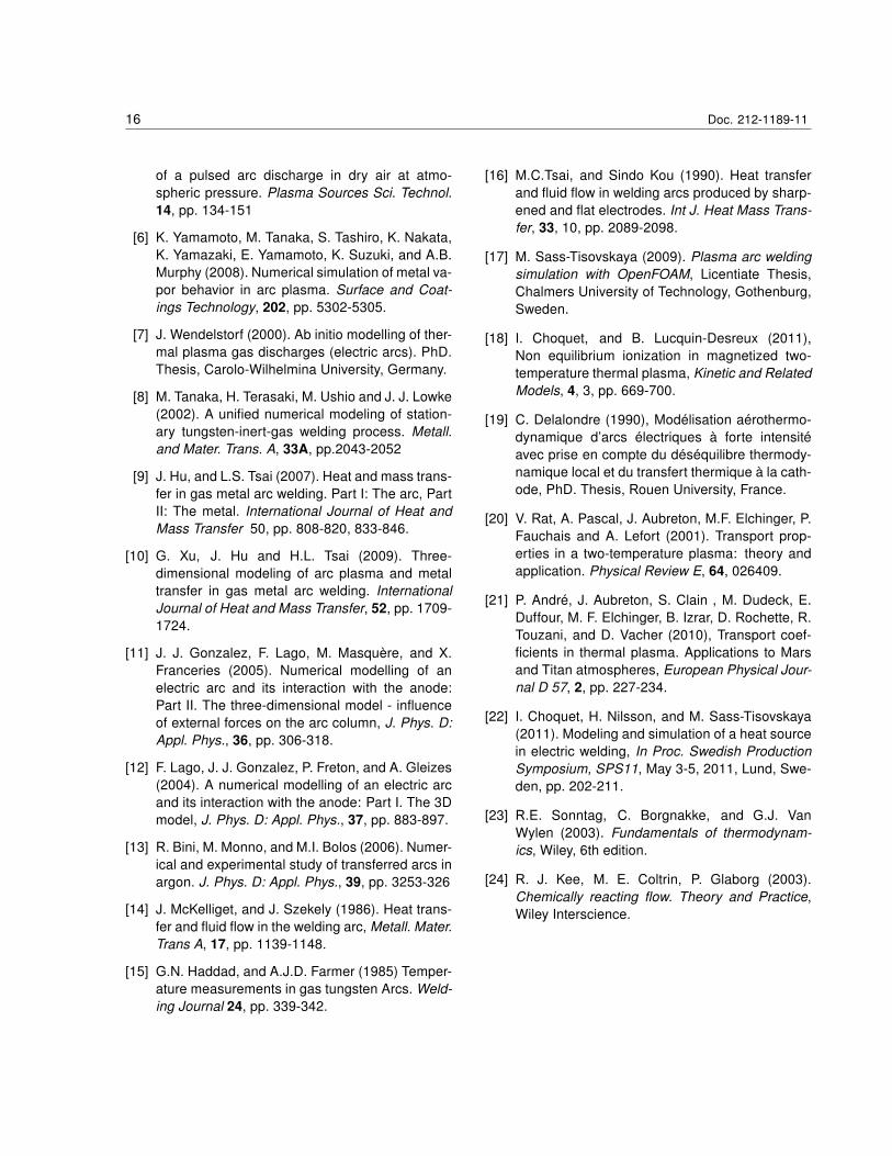
mum arc temperature. Also, compared to case a, themaximum temperature of case b is much closer to themaximum temperature observed experimentally. Thethermal boundary condition on the anode has almostno influence on the maximum arc temperature. How-ever, it can significantly affect the heat transferred tothe anode base metal, as it significantly changes thetemperature close to the anode.Finally, Fig. 16 and 17 show that the velocity alongthe symmetry axis and the pressure force on thebase metal are significantly changed for each varia-tion tested on the anode and cathode boundary con-ditions.
Figure 15: Influence of the anode and cathodeboundary conditions on the temperature along the
symmetry axis.
Figure 16: Influence of the anode and cathodeboundary conditions on the velocity along the
symmetry axis.
Figure 17: Influence of the anode and cathodeboundary conditions on the pressure on the base
metal.
Doc. 212-1189-11 15
4 CONCLUSION
This study focused on the modeling and simulation ofan electric arc heat source, coupling thermal fluid me-chanics with electromagnetics. The model, valid forthe plasma core, was implemented in the open sourcesoftware OpenFOAM. Different approaches were con-sidered for modeling the electromagnetic fields:
i) the three-dimensional approach,
ii) the two-dimensional axi-symmetric approach,
iii) the electric potential formulation, and
iv) the magnetic field formulation as described byRamírez et al. [1].
Models i) to iii) reduce to the same quasi one-dimensional limit for an axi-symmetric configurationwith negligible radial current density, contrary to modeliv). Model iv) is a non-closed version of the axi-symmetric model. It does not account for the chargeconservation equation. On the contrary, the elec-tric potential formulation is closed with a quasi one-dimensional closure relation. Models ii) to iv) cannotrepresent the same physics when the radial currentdensity is significant, such as for a short arc or anelectrode tip with a conical shape.
The electromagnetic solver was tested against the an-alytic solution of an infinite electric rod using models i)to iii). The solutions are in perfect agreement.The coupled solver was tested against experimentalmeasurements for GTAW with argon shielding gas anda short arc (2 mm). The numerical solution for the az-imuthal component of the magnetic field then signifi-cantly differs when applying the electric potential for-mulation iii). This approach indeed neglects the radialcurrent density component. For axi-symmetric con-figurations with non-negligible radial effects, such asshort arcs, this simplification is not everywhere justi-fied. The numerical results obtained using models i)and ii) show a good agreement with the experimentaldata when such comparisons can be made.
Difficulty were met in setting appropriate boundaryconditions, either because of lack of experimentaldata, or because of a too large freedom for extrapolat-ing available experimental data up to the anode andcathode surface. In addition different possible con-ditions significantly affect the simulation results, suchas the plasma arc temperature and velocity. The tem-perature and current density distribution on the elec-
trode surface should thus be calculated rather thanset, to enhance the predictive capability of the sim-ulation model. The solution of the temperature andelectromagnetic fields inside the anode and cathode,and the modeling of the plasma arc sheath doing thecoupling with the plasma core, will thus be included inthe forthcoming development of the simulation model.
Acknowledgment: The authors thank Prof. JacquesAubreton and Prof. Marie-Françoise Elchinger forthe data tables of thermodynamic and transport prop-erties they did provide. This work was supportedby KK-foundation in collaboration with ESAB, VolvoConstruction Equipment and SSAB. Håkan Nilssonwas in this work financed by the Sustainable Produc-tion Initiative and the Production Area of Advance atChalmers. These supports are gratefully acknowl-edged.Grateful acknowledgement is made to the WeldingJournal for permission to reproduce figure 5 from thepaper "Temperature Measurements in Gas TungstenArcs" (1985, 64(12)).
5 References
[1] M.A. Ramírez , G. Trapaga and J. McKelliget(2003). A comparison between two different nu-merical formulations of welding arc simulation.Modelling Simul. Mater. Sci. Eng, 11, pp. 675-695.
[2] L. Lindgren, B. Babu, C. Charles, and D. Wed-berg (2010). Simulation of manufacturing chainsand use of coupled microtructure and constitu-tive models. Finite Plasticity and Visco-plasticityof Conventional and Emerging Materials, Khan,A. S. and B. Farrokh, (red.). NEAT PRESS, 4 s.
[3] A. Kumar, and T. DebRoy (2007). Heat transferand fluid flow during Gas-Metal-Arc fillet weldingfor various joint configurations and welding posi-tions. The minerals, metals and materials societyand ASM International.
[4] K.C. Hsu, K. Etemadi and E. Pfender (1983).Study of the free-burning high intensity argon arc,J. Appl. Phys., 54, pp. 1293-1301.
[5] Y. Tanaka, T. Michishita and Y. Uesugi (2005).Hydrodynamic chemical non-equilibrium model
16 Doc. 212-1189-11
of a pulsed arc discharge in dry air at atmo-spheric pressure. Plasma Sources Sci. Technol.14, pp. 134-151
[6] K. Yamamoto, M. Tanaka, S. Tashiro, K. Nakata,K. Yamazaki, E. Yamamoto, K. Suzuki, and A.B.Murphy (2008). Numerical simulation of metal va-por behavior in arc plasma. Surface and Coat-ings Technology, 202, pp. 5302-5305.
[7] J. Wendelstorf (2000). Ab initio modelling of ther-mal plasma gas discharges (electric arcs). PhD.Thesis, Carolo-Wilhelmina University, Germany.
[8] M. Tanaka, H. Terasaki, M. Ushio and J. J. Lowke(2002). A unified numerical modeling of station-ary tungsten-inert-gas welding process. Metall.and Mater. Trans. A, 33A, pp.2043-2052
[9] J. Hu, and L.S. Tsai (2007). Heat and mass trans-fer in gas metal arc welding. Part I: The arc, PartII: The metal. International Journal of Heat andMass Transfer 50, pp. 808-820, 833-846.
[10] G. Xu, J. Hu and H.L. Tsai (2009). Three-dimensional modeling of arc plasma and metaltransfer in gas metal arc welding. InternationalJournal of Heat and Mass Transfer, 52, pp. 1709-1724.
[11] J. J. Gonzalez, F. Lago, M. Masquère, and X.Franceries (2005). Numerical modelling of anelectric arc and its interaction with the anode:Part II. The three-dimensional model - influenceof external forces on the arc column, J. Phys. D:Appl. Phys., 36, pp. 306-318.
[12] F. Lago, J. J. Gonzalez, P. Freton, and A. Gleizes(2004). A numerical modelling of an electric arcand its interaction with the anode: Part I. The 3Dmodel, J. Phys. D: Appl. Phys., 37, pp. 883-897.
[13] R. Bini, M. Monno, and M.I. Bolos (2006). Numer-ical and experimental study of transferred arcs inargon. J. Phys. D: Appl. Phys., 39, pp. 3253-326
[14] J. McKelliget, and J. Szekely (1986). Heat trans-fer and fluid flow in the welding arc, Metall. Mater.Trans A, 17, pp. 1139-1148.
[15] G.N. Haddad, and A.J.D. Farmer (1985) Temper-ature measurements in gas tungsten Arcs. Weld-ing Journal 24, pp. 339-342.
[16] M.C.Tsai, and Sindo Kou (1990). Heat transferand fluid flow in welding arcs produced by sharp-ened and flat electrodes. Int J. Heat Mass Trans-fer, 33, 10, pp. 2089-2098.
[17] M. Sass-Tisovskaya (2009). Plasma arc weldingsimulation with OpenFOAM, Licentiate Thesis,Chalmers University of Technology, Gothenburg,Sweden.
[18] I. Choquet, and B. Lucquin-Desreux (2011),Non equilibrium ionization in magnetized two-temperature thermal plasma, Kinetic and RelatedModels, 4, 3, pp. 669-700.
[19] C. Delalondre (1990), Modélisation aérothermo-dynamique d’arcs électriques à forte intensitéavec prise en compte du déséquilibre thermody-namique local et du transfert thermique à la cath-ode, PhD. Thesis, Rouen University, France.
[20] V. Rat, A. Pascal, J. Aubreton, M.F. Elchinger, P.Fauchais and A. Lefort (2001). Transport prop-erties in a two-temperature plasma: theory andapplication. Physical Review E, 64, 026409.
[21] P. André, J. Aubreton, S. Clain , M. Dudeck, E.Duffour, M. F. Elchinger, B. Izrar, D. Rochette, R.Touzani, and D. Vacher (2010), Transport coef-ficients in thermal plasma. Applications to Marsand Titan atmospheres, European Physical Jour-nal D 57, 2, pp. 227-234.
[22] I. Choquet, H. Nilsson, and M. Sass-Tisovskaya(2011). Modeling and simulation of a heat sourcein electric welding, In Proc. Swedish ProductionSymposium, SPS11, May 3-5, 2011, Lund, Swe-den, pp. 202-211.
[23] R.E. Sonntag, C. Borgnakke, and G.J. VanWylen (2003). Fundamentals of thermodynam-ics, Wiley, 6th edition.
[24] R. J. Kee, M. E. Coltrin, P. Glaborg (2003).Chemically reacting flow. Theory and Practice,Wiley Interscience.