elec 5570 control systems and design benjamin chong – room g62 email: [email protected]
TRANSCRIPT
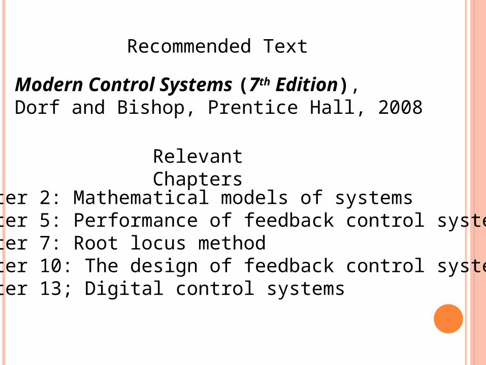
Recommended Text
Modern Control Systems (7th Edition), Dorf and Bishop, Prentice Hall, 2008
Relevant Chapters
Chapter 2: Mathematical models of systemsChapter 5: Performance of feedback control systemsChapter 7: Root locus methodChapter 10: The design of feedback control systemsChapter 13; Digital control systems

CHAPTER 1 – SYSTEM MODELLING
A simple position control system
r(t)
PlantControllerController output
= Plant input
(t)
Power Amp.
K
R2
R1
R1
RaLa
Va
Pot.
Kt+
+
R
R

CHAPTER 1 – SYSTEM MODELLING
Development of a Control SystemRepresentation of plantRequirements/specificationsDesign techniquesVerification/validation Implementation and testing

CHAPTER 1 – SYSTEM MODELLING
Plant (The system to be controlled)
Electrical, Mechanical, Aeronautical, Chemical (or combination)
Mathematical Modelling (Differential equations, transfer functions)
Model simplification (Identification of parts which can be neglected)
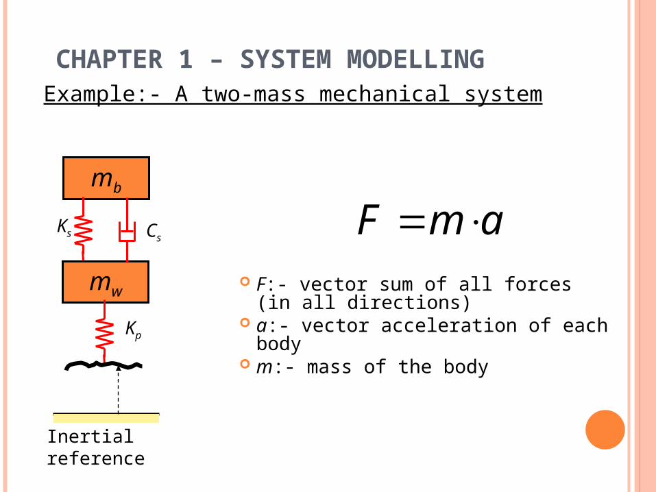
CHAPTER 1 – SYSTEM MODELLINGExample:- A two-mass mechanical system
F:- vector sum of all forces (in all directions)
a:- vector acceleration of each body
m:- mass of the body
amF mb
mw
Ks Cs
Kp
Inertial reference

CHAPTER 1 – SYSTEM MODELLINGExample:- A two-mass mechanical system
mb
mw
Ks Cs
Kp
xb
xw
xg
Inertial reference
Fs
Fp cFFxm spww
sbb Fxm
Equations of motion
)( wgpp xxKF )()( bwsbwss xxCxxKF
Forces on the wheel and suspension

CHAPTER 1 – SYSTEM MODELLINGExample:- A two-mass mechanical system
Transfer function from xg to xb
gpbsbswpswsww xKxKxCxKKxCxm )(
Equations of Motion
0 wswsbsbsbb xKxCxKxCxm
gpbsswpssw xKsXKsCsXKKsCsm )()()(])[( 2
0)()()()( 2 sXKsCsXKsCsm wssbssb
In the s-domain – take Laplace transforms
spspswpbsbwbswb
spsp
KKsCKsKmKmKmsmmCsmm
KKsCKsH
234 )()(
)(

CHAPTER 1 – SYSTEM MODELLINGExample:- An electric circuit
RR Riv LL i
dt
dLv dti
Cv CC
1
L
RCva
• Kirchhoff’s laws (voltage and current)
• Relations between voltage and current for R, L, C components
0 kv enterleave ii
)()( sRIsV RR )()( sLsIsV LL )(1
)( sICs
sV CC

CHAPTER 1 – SYSTEM MODELLINGExample:- An electric circuit
L
RCva
)( LL idt
dLv
)( CRRa iidt
dLvv ))(( CR v
dt
dCi
dt
dL
CRL iii
0 aRL vvv
RRRa vLCiLvv

CHAPTER 1 – SYSTEM MODELLINGExample:- An electric circuit
L
RCva
aRRR vvvR
LvLC
Hence:
In the s-domain:
aR vvsR
LLCs )1( 2

CHAPTER 1 – SYSTEM MODELLINGExample:- A position control system
r(t)
k + dtid
L + Ri = v ta
aaaa Electrical part
ik = B dt
dJ at
Mechanical part
Power Amp.
K
R2
R1
R1
RaLa
Va
Pot.
kt+
+
R
R (t)ia

CHAPTER 1 – SYSTEM MODELLINGExample:- A position control system
)()()( sIk = sB Js at
In the s-domain:-
)()()()( sk +sI RsL = sV taaaa
)())((
)( sV k + L s+ R sJ+ B
k = s a2taa
t )())((
sV k + R sJ+ B
k a2ta
t
)(
)(1
)(sV
k + BR
JR s+
k + BR
k
a
2ta
a
2ta
t
)(1
sV sT+
k = a

)()1(
)( sV sTs
k = s a
The transfer function between angular armature voltage and output velocity is therefore given by
)1()(
sTs
kK = sG
If we now include the voltage gain of the amplifier,the transfer function of the forward path (in green) is
CHAPTER 1 – SYSTEM MODELLING

Transfer Function – Input/Output Relationship
CHAPTER 1 – SYSTEM MODELLING
Another approach which employs state-space modelling technique can be used.
-Derived by simultaneously manipulating multiple differential equations- This approach is straightforward for systems of 2 order or less
- This approach can also be applied to higher order systems - Can be used when there are multiple input/outputs

CHAPTER 1 – SYSTEM MODELLING
-a method for describing a system in terms of a set of first order linear differential equations.
In the general form they can be expressed as
uD + xC = y
uB + xA = x
State-space modelling technique

CHAPTER 1 – SYSTEM MODELLING
State-space modelling technique
uD + xC = y
uB + xA = x
nx
x
x 1
where is an n 1 vector of state variables
pu
u
u 1
my
y
y 1is a p 1 vector
of inputs is an m 1 vector of outputs
A is an n n matrix, B is an n p matrix, C is an m n matrix, D is an m p matrix.

State-space modelling technique (single-input, single-output (SISO) system)
CHAPTER 1 – SYSTEM MODELLING
p = m =1 We have
We can write B = b (nx1 column vector), C = c which is a 1 n row vector and d is scalar, i.e.
ud +xc =y
ub + xA = x
CHAPTER 1 – SYSTEM MODELLING
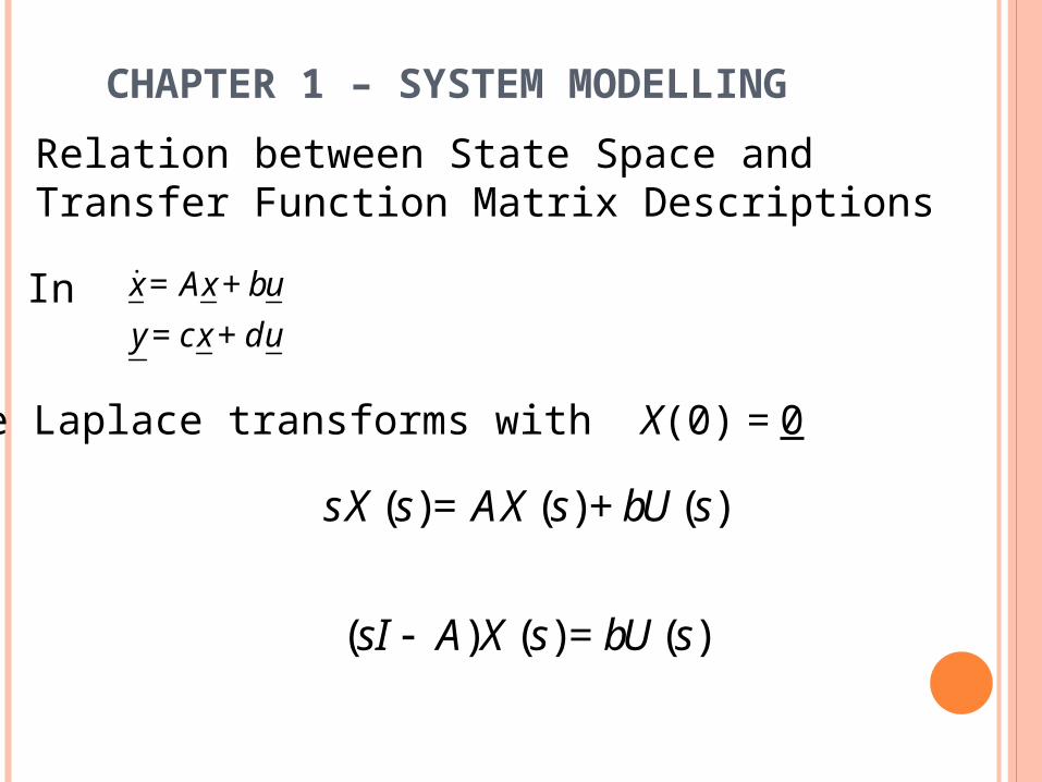
Relation between State Space and Transfer Function Matrix Descriptions
Inud + xc = y
ub + xA = x
take Laplace transforms with X(0) = 0
)()()(
)()()(
sUb =sXA sI
sUb + sXA = sXs

CHAPTER 1 – SYSTEM MODELLING
Hence)()()( 1 sbUA sI = sX
and
)()()()( 1 sdU + sbUA sIc = sY
Hence
)()()(
)()()( 1
sU sG = sY
sU d + bA sIc = sY

CHAPTER 1 – SYSTEM MODELLING
)()()(
)()()( 1
sUsG = sY
sU d + bA sIc = sY
Application of state-space modelling technique fortransfer function derivation
k Riv = dtid
L taa aa
a
B ik = dt
dJ at
ai
x
xx
2
1
y
vu a
ud + xc = y
ub + xA = x
Input/outputState variable
Note: Input is independent

CHAPTER 1 – SYSTEM MODELLING
Application of state-space modelling technique fortransfer function derivation
k Riv = dtid
L taa aa
a
B ik = dt
dJ at
JB
Jk
Lk
LR
At
a
t
a
a
0
1aLb
0 ,10 dc
)()()(
)()()( 1
sU sG = sY
sU d + bA sIc = sY ud + xc = y
ub + xA = x

CHAPTER 1 – SYSTEM MODELLING
Application of state-space modelling technique fortransfer function derivation
0
1aLb 0 ,10 dc
a
at
a
t
taa
a
LRsJ
kL
kJ
Bs
kBJsRsL
JLAsI
21
)()()(
)()()( 1
sU sG = sY
sU d + bA sIc = sY

CHAPTER 1 – SYSTEM MODELLING
Application of state-space modelling technique fortransfer function derivation
)(
)(
)()(
2
1
sV
s
kBJsRsL
k
d + bA sIcsG
ataa
t
)()()(
)()()( 1
sU sG = sY
sU d + bA sIc = sY