elec 372 laboratory manual - concordia universityrealtime/elec372/docs/elec372_lab... · laboratory...
TRANSCRIPT
ELEC 372 - FUNDAMENTALS OF CONTROL SYSTEMS
LABORATORY MANUAL
September 2016
Department of Electrical & Computer Engineering
Concordia University
1515 St. Catherine West, S-EV005.139, Montreal, Quebec, Canada H3G 2W1
http://www.ece.concordia.ca/~realtime

ELEC372 Lab Manual Department of ECE
1
PLEASE READ IMPORTANT INFORMATION REGARDING
EMERGENCY PROCEDURES GIVEN ON THE LAST PAGE!
ELEC 372 - FUNDAMENTALS OF CONTROL SYSTEMS
LABORATORY MANUAL N.Suresh
Revised by: Dan Li, Maria Enayat,
Shahin Hashtrudi Zad
ECE Control Systems Laboratory
Dept. of Electrical & Computer Engineering
CONCORDIA UNIVERSITY

ELEC372 Lab Manual Department of ECE
2
Table of Contents Table of Contents ..................................................................................................................................... 2
1 GENERAL INSTRUCTIONS ................................................................................................................. 5
1.1 INTRODUCTION ........................................................................................................................ 5
1.2 LAB REGULATIONS .................................................................................................................... 5
1.3 RULES OF CONDUCT TO BE OBSERVED IN THE LAB ................................................................. 6
1.4 MISSED LABS AND MAKEUP PROCEDURE ................................................................................ 6
1.5 EXPERIMENT OUTLINE .............................................................................................................. 6
1.6 LAB TEST ................................................................................................................................... 7
1.7 MARKING GUIDELINE ............................................................................................................... 7
1.8 REFERENCE ............................................................................................................................... 7
2 LABORATORY EQUIPMENT OVERVIEW ............................................................................................ 8
2.1 GENERAL DESCRIPTION ............................................................................................................ 8
2.2 ROTATIONAL-MOTION ASSEMBLY ........................................................................................... 8
2.3 CONTROL BOX ........................................................................................................................ 11
2.4 WORKSTATION ....................................................................................................................... 11
2.5 ECP EXECUTIVE CONTROL PROGRAM .................................................................................... 11
2.6 DATA FOR LAB REPORTS ......................................................................................................... 17
2.7 SAFETY PROCEDURES ............................................................................................................ 18
3 EXPT #1: FAMILIARIZATION WITH EXPERIMENT SYSTEMS ............................................................ 19
3.1 OBJECTIVE ............................................................................................................................... 19
3.2 INTRODUCTION ...................................................................................................................... 19
3.3 ECP MODEL 220 SYSTEM ........................................................................................................ 21
3.4 PLOT DATA WITH MATLAB ..................................................................................................... 23
3.5 OPEN-LOOP TEST and SIMULATION ....................................................................................... 24
4 EXPT #2: SYSTEM IDENTIFICATION ................................................................................................ 27
4.1 OBJECTIVE ............................................................................................................................... 27
4.2 INTRODUCTION ...................................................................................................................... 27
4.3 PLANT PARAMETER and SYSTEM MODELING ........................................................................ 29
5 EXPT #3: IMPROVING SYSTEM PERFORMANCE ............................................................................. 36
5.1 OBJECTIVE ............................................................................................................................... 36
5.2 INTRODUCTION ...................................................................................................................... 36

ELEC372 Lab Manual Department of ECE
3
5.3 PID CONTROL .......................................................................................................................... 39
5.4 STEADY STATE ERROR ANALYSIS ............................................................................................ 41
5.5 DISTURBANCE ATTENUATION ................................................................................................ 43
6 EXPT #4: TRANSIENT AND FREQUENCY RESPONSE ....................................................................... 46
6.1 OBJECTIVE ............................................................................................................................... 46
6.2 INTRODUCTION ...................................................................................................................... 46
6.3 CLOSED-LOOP TRANSIENT RESPONSE .................................................................................... 49
6.4 OPEN-LOOP FREQUENCY RESPONSE ...................................................................................... 51
6.5 CLOSED-LOOP FREQUENCY RESPONSE .................................................................................. 54
7 EXPT #5: LAG AND LEAD COMPENSATION .................................................................................... 57
7.1 OBJECTIVE ............................................................................................................................... 57
7.2 INTRODUCTION ...................................................................................................................... 57
7.3 COMPENSATOR DESIGN ......................................................................................................... 58
7.4 LEAD COMPENSATION ............................................................................................................ 63
7.5 LAG COMPENSATION.............................................................................................................. 64
APPENDIX-A: EXPECTATIONS OF ORIGINALITY ...................................................................................... 65
ELEC372 Lab Manual Department of ECE
4
Figure 2.1: Basic system components ...................................................................................................... 8
Figure 2.2: Rotational-motion Assembly .................................................................................................. 9
Figure 2.3: Actual arrangement of turntable components .................................................................... 10
Figure 2.4: ECP Background Screen ........................................................................................................ 12
Figure 2.5: Available Closed-Loop System Configurations ..................................................................... 13
Figure 2.6: Control Algorithm selection screen ...................................................................................... 13
Figure 2.7: Setup an algorithm ............................................................................................................... 14
Figure 2.8: Available Trajectory .............................................................................................................. 15
Figure 2.9: Setup Data Acquisition ......................................................................................................... 16
Figure 2.10: Setup Plot ........................................................................................................................... 16
Figure 3.1: DC Motor Open-loop Diagram ............................................................................................. 19
Figure 3.2: ECP 220 System Configuration ............................................................................................. 20
Figure 4.1: A closed-loop configuration ................................................................................................. 27
Figure 4.2: Plan Rotation Inertia ............................................................................................................. 28
Figure 5.1: Closed-loop Configuration .................................................................................................... 36
Figure 5.2: Unity Feedback System ........................................................................................................ 37
Figure 5.3: Disturbance control .............................................................................................................. 39
Figure 6.1: Typical unit response of a system ........................................................................................ 46
Figure 6.2: The relation between PO and ζ ............................................................................................ 47
Figure 6.3: System Configuration ........................................................................................................... 47
Figure 6.4: Bode Plots ............................................................................................................................. 48
Figure 6.5: Polar Plots ............................................................................................................................ 49
Figure 7.1: PID+Notch Configuration ...................................................................................................... 58

ELEC372 Lab Manual Department of ECE
5
1 GENERAL INSTRUCTIONS
1.1 INTRODUCTION This manual provides the operating instructions in a simplified form and leads ELEC372 students through a prescribed set of experiments aimed at demonstrating the basic principles of feedback control systems.
It is essential that students read these preliminary sections in order to understand the purpose of each experiment. A brief tutorial, pertaining to the work to be done, will also be given by the lab instructor at the start of each lab. In addition, students should prepare ahead for each lab and make an attempt to understand each experiment in order to gain maximum benefit from the course.
• To illustrate the material that is the subject matter of ELEC372 course by experiment. Specifically, to acquaint students with a practical control system. An electromechanical angular-position control system is used as an example.
• To familiarize students with practical transient-response and frequency-response testing of a control system, and to investigate various controller configurations.
• To give the students the opportunity to practice engineering report writing and teamwork.
• To train the students to use engineering tool, MATLAB, to create and extend its functions as necessary. MATLAB is an interactive program for numerical computation and data visualization; it is used extensively by control engineers for analysis and design.
1.2 LAB REGULATIONS • The lab has 8 numbered stations with a maximum of 2 students per station. Each station group
must use the same station for the entire sessions.
• Experiments will be performed in five sessions in the sequence given in the Lab schedule sheet which will be distributed to students in class before labs start. Each lab will meet every alternate week. Every group member must participate in performing the experiments.
• Every student must prepare and submit an individual report to the lab instructor at the subsequent lab session. Marked reports will be returned at the subsequent session. The marking guideline is given later in the manual. Late submissions will be penalized. The deadline for the final report (#5), which may be less than a week, will be provided by the lab instructor.
• Reports should be concise, original and meaningful. Every report must carry the signed and dated ‘Expectations of Originality’ statement: “I certify that this submission is my original work and meets the Faculty's Expectations of Originality” required by ENCS regulations. A copy of the ENCS document is provided in the Appendix of the manual. Wherever possible, data calculated or obtained in the lab must be authenticated by the lab instructor’s signature/initials. Students are encouraged to use results from various available mathematical and control systems simulation software in their reports.

ELEC372 Lab Manual Department of ECE
6
• Final reports should be reclaimed from the lab instructor at the end of the session.
• Unclaimed reports will be retained only for a period of three months after the end of the session, after which they will not be available.
1.3 RULES OF CONDUCT TO BE OBSERVED IN THE LAB • Students are expected to treat the lab equipment and the instructor with due respect.
Disciplinary action will be taken against any student caught misusing the lab such as making marks on benches or other equipment.
• Students must show seriousness in performing the lab and not be a source of disturbance to neighboring stations. Cell phones must be switched off and students are not allowed to exit the lab to hold cell-phone conversations.
• Water-bottles or other liquid containers are not allowed in the workspace. Eating, drinking, and smoking are strictly forbidden in the lab by university regulations. All clothing, bags, etc. must be put away from the work area. Keep the workspace clean.
• At the end of each session, make sure that all scrap papers, pens, etc. are removed and that the lab equipment is switched off according to procedures given later.
• Fire or Other Emergencies: In the event of a fire or other emergency requiring evacuation of the building, students must follow the lab instructor’s directives and immediately leave the building via the stairwells. There are two stairwells closed to the lab location and these are indicated on a map found in the lab.
Please also read the emergency procedures given on the last page of this manual.
1.4 MISSED LABS AND MAKEUP PROCEDURE Only one lab absence* is permitted. If you miss more than one lab, you are not likely to obtain the average of 50% in the lab, which is required to pass the course. A student who misses a lab must attend another lab within the same experimental cycle to make up for the missed experiment and must immediately email both her/his lab TA and the Lab coordinator about the substitution. In general, a lab missed due to unavoidable grave circumstance, such as accident or illness, may be disregarded in calculating the average grade provided that an authentic document (police report, doctor’s or hospital certificate etc.) is furnished.
*Note: Expt#1 is a ‘familiarization’ experiment and should not be missed. No makeup will be given for Expt#1 after its cycle has ended.
1.5 EXPERIMENT OUTLINE The five experiments to be performed in the laboratory component of the course are given in the following sections. All five experiments are designed to demonstrate the content taught in ELEC372:
• EXPT #1: FAMILIARIZATION WITH EXPERIMENT SYSTEMS • EXPT #2: SYSTEM IDENTIFICATION

ELEC372 Lab Manual Department of ECE
7
• EXPT #3: IMPROVING SYSTEM PERFORMANCE • EXPT #4: TRANSIENT AND FREQUENCY RESPONSE • EXPT #5: LAG AND LEAD COMPENSATION
Although the lab experiments are intended to complement the classroom lectures, the limited time available during the semester will certainly cause the subject matter of the experiments to be ahead of the topics being taught in class at any given time. In order to somewhat alleviate this situation, each experiment in this manual is preceded by a short 'tutorial' which attempts to explain the particular topic being investigated. Relevant tutorial material is also given in the introduction part of each experiment.
1.6 LAB TEST The lab test is a 45-minute test based on individuals, not for groups, normally in the week following the last experiment. The students will work with a question paper labeled #1, #2, #3 or #4. Only the Lab Manual and an ENCS-approved calculator are allowed. All other materials should be put away as in a written exam.
1.7 MARKING GUIDELINE The lab marks count for 15 percent in the ELEC372 course grading scheme. The average of the five labs will be reported on a maximum of 10 and the lab test on a maximum of 5.
Lab reports will be graded on a scale of 10 with the approximate percentage weightings shown:
Table 1.1: Marking guideline
1 Participation: Attendance and Lab Performance [Good performance is an indication of Being well- prepared for the experiment to be done]
20%
2 Organization and Presentation: Coherence, Proper Tabulation, Calculations, Simulations, Computer-drawn or neatly hand drawn graphs
30%
3 Discussion and Summary: Technical discussion of obtained results, error calculations, experimental / theoretical correlations, Meaningful conclusion (summary of what was learnt etc.)
50%
1.8 REFERENCE i. Modern Control Systems, Richard C. Dorf and Robert H. Bishop, 11th Edition, Prentice Hall.
ii. Manual for ECP Model 220, Instructor’s Edition, ECP Control Systems, 1995 iii. MATLAB R2014b on-line Help. www.matlab.com
ELEC372 Lab Manual Department of ECE
8
2 LABORATORY EQUIPMENT OVERVIEW
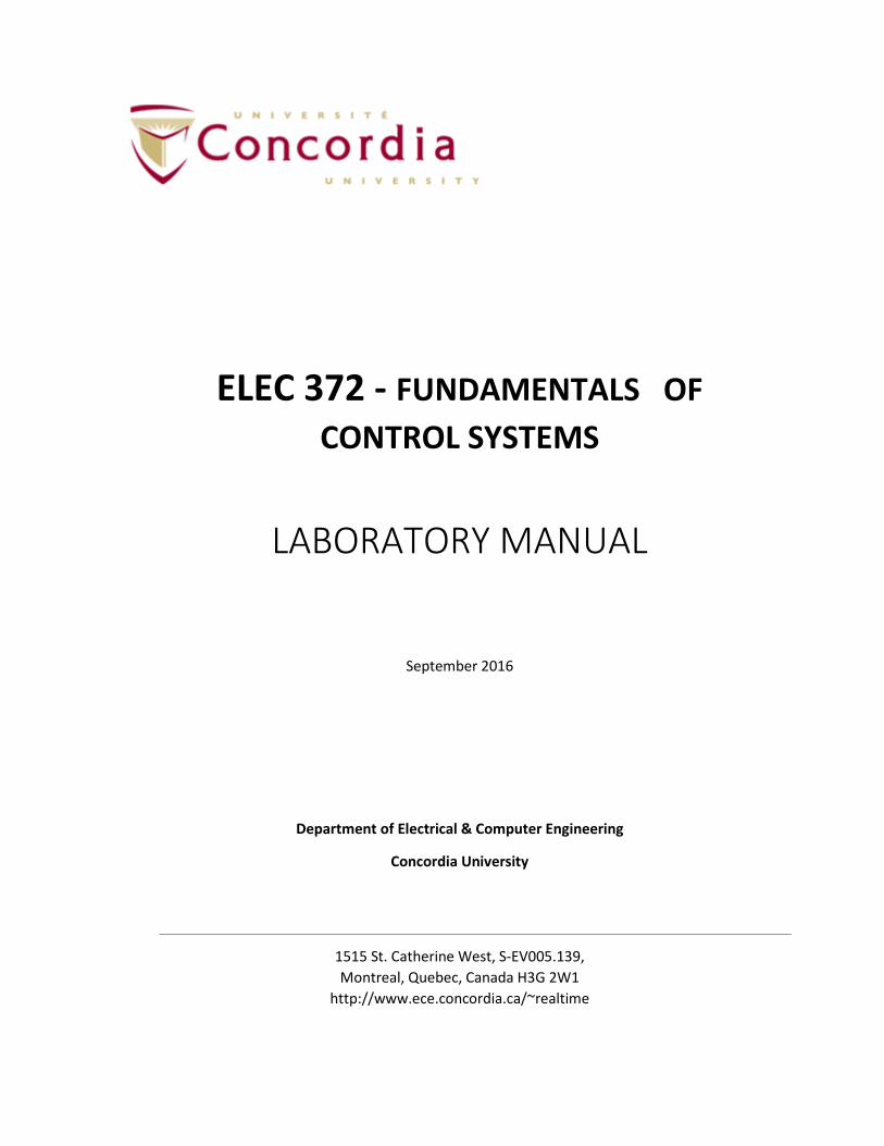
2.1 GENERAL DESCRIPTION The laboratory equipment used in this Lab is an ECP Model 220 Industrial Emulator which is a rotational motion control system designed for teaching purposes by Educational Control Products (ECP systems) company. The components of the system are shown schematically in Figure 2.1. The system is driven by a digital real-time controller with a digital computer (PC) as an interface. The ‘plant’ is a rotational-motion assembly consisting of a motor-driven set of two turntables (called ‘disks’ hereafter) which are coupled by means of selectable toothed belts and pulleys. Additional weights may be symmetrically added to the turntables thereby increasing their effective rotational inertia. Once the mechanical configuration (i.e. belts, pulleys, weights) of the system is selected, the ‘plant’ consisting of the motor/turntable assembly can be represented by a first-order rotational friction/inertia model described in experiment (1). The two turntables are provided with optical digital-encoders which measure their position, velocity and acceleration. The ‘control box’ contains all the drive and measurement circuits required for actuating the system. A desktop PC, which contains a digital controller as well as ECP executive program, is used to complete the closed loop system. Controller and control-parameter selection, data entry, and output display selection are all made through the peripherals (keyboard/mouse/monitor) of the PC. Thus, for any given mechanical configuration, the remaining operations are entirely computer-menu-driven with a graphical-user-interface. Although the control signal is implemented through digital means ('sampled data'), it can physically emulate an analog system, which is the mode that is utilized for the purposes of this lab.
PC Monitor
CONTROL BOX
Keyboard
PC
Mouse
Rotational Motion Assembly
RED Abort ButtonBLACK ‘ON’ Button
Turntables
Figure 2.1: Basic system components
2.2 ROTATIONAL-MOTION ASSEMBLY This unit basically consists of two belt-driven metal turntables (hereafter called ‘drive’ and ‘load’ disk) which are shown schematically in Figure 2.1: Basic system components. The two disks are radially slotted, so that two or four symmetrically-spaced, brass weights may be attached in order to change (increase) their rotational inertia. In the lab setup, the positions of these weights are fixed at the maximum radius of each turntable. The two disks are coupled using toothed-belts and pulleys through an intermediate ‘speed-reduction’ (SR) assembly. The SR unit has mechanisms to provide backlash, if

ELEC372 Lab Manual Department of ECE
9
required. Backlash (also known as “Dead Zone” or “Deadband”) is a non-linearity which typically occurs in system transmission links such as gear trains and/or ‘rack & pinion’ assemblies. The effect of backlash is seen as a short interval of inactivity (i.e. no output) whenever the direction of motion is reversed. It is a nonlinear effect. Since the experiments in this lab deal with ‘linear’ systems, the backlash setting facility is not used in the lab setup.
DRIVE MOTOR
DISTURBANCE MOTOR
4 : 1
1 : 1
LOAD DISK DRIVE DISK
ADDED WEIGHTS(Bolted On)
Typical Toothed Belts
SR ASSEMBLY
ENCODER # 1ENCODER # 2
Figure 2.2: Rotational-motion Assembly
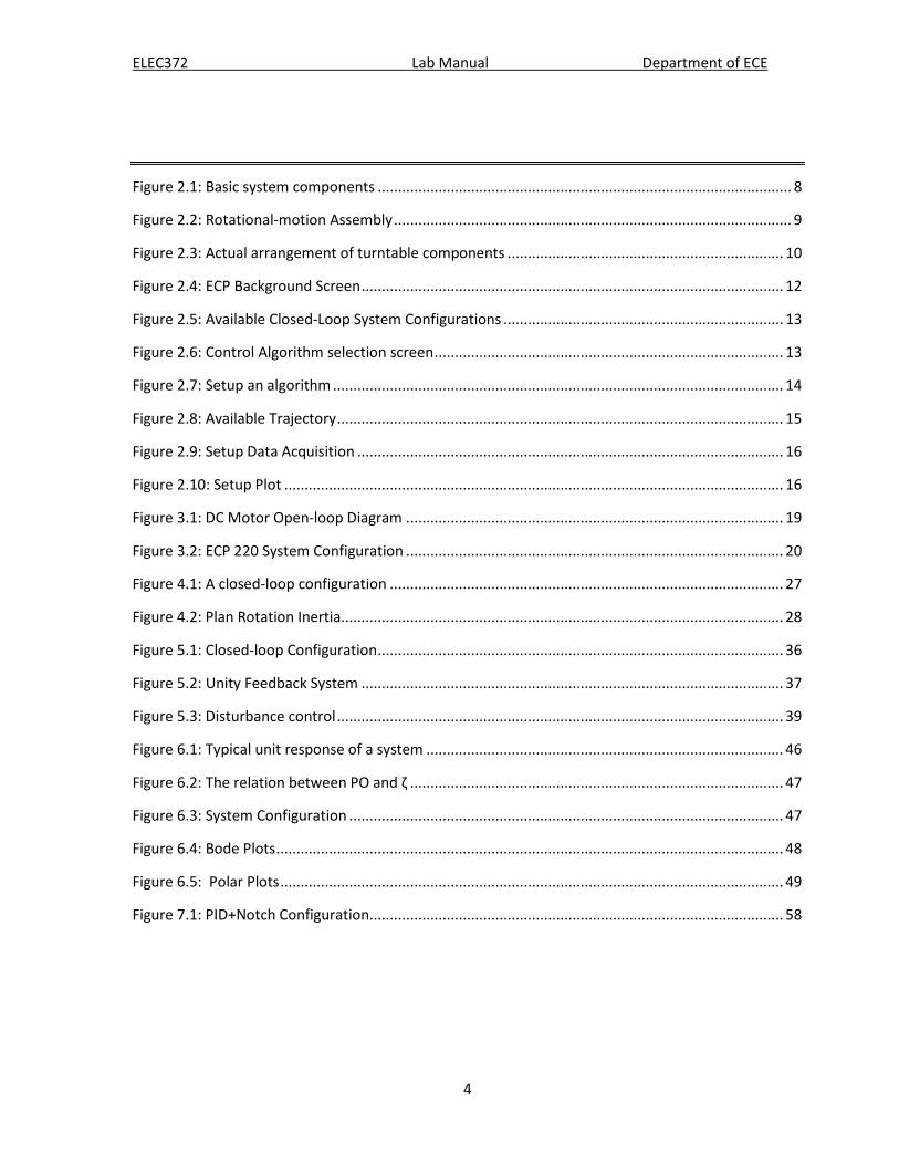
Speed reduction ratios can be changed in the system by selecting interchangeable pulleys in the SR assembly. The equipment also permits a flexible belt to be used between the SR assembly and the ‘load’ table, for advanced studies on “flexible-drive control systems”. If the flexible belt is not used and if the backlash set is ‘zero’, then the rotational components are considered to form a rigid (as opposed to flexible) system. The drive disk is driven by a brushless DC drive motor through a 1:1 belt/pulley coupling. Another brushless DC motor, called the ‘disturbance motor’, is coupled to the ‘load’ disk through a 4:1 belt/pulley. Various disturbance signals such as step or sinusoidal (or other user-defined functions) can be introduced into the system through this motor. The disturbance motor also allows an equivalent viscous friction to be introduced at the load disk location.
The experiments described in this manual assume a rigid system with all inertias reflected to the drive disk axis at Encoder#1, with an overall reduction ratio of 4:1 (i.e. 4 revolutions of the drive disc at Encoder#1 result in 1 revolution of the load disk at Encoder#2). The encoder outputs are points of origin of feedback signals, so that a feedback loop may be ‘closed around’ either of the encoders. In the lab experiments, the loop is closed around encoder #1 (at the drive disk), and all inertias and friction is ‘referred’ to the drive-disk side of the rotational assembly. All the above components are mounted within a metal frame which can be oriented horizontally or vertically; in this lab the frame is used with the rotational axes pointing in the vertical direction only, so that gravitational torques will not be present.
The actual arrangement of the motional components is shown in Figure 2.3.
ELEC372 Lab Manual Department of ECE
10
Figure 2.3: Actual arrangement of turntable components
ELEC372 Lab Manual Department of ECE
11
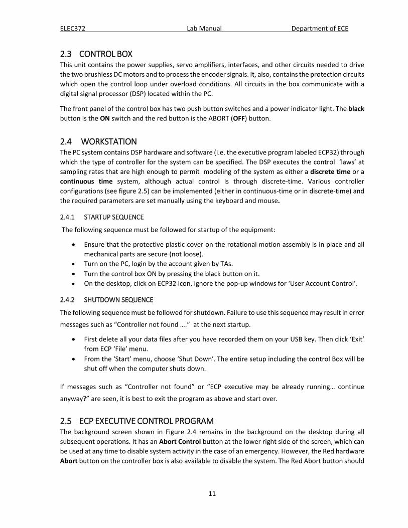
2.3 CONTROL BOX This unit contains the power supplies, servo amplifiers, interfaces, and other circuits needed to drive the two brushless DC motors and to process the encoder signals. It, also, contains the protection circuits which open the control loop under overload conditions. All circuits in the box communicate with a digital signal processor (DSP) located within the PC.
The front panel of the control box has two push button switches and a power indicator light. The black button is the ON switch and the red button is the ABORT (OFF) button.
2.4 WORKSTATION The PC system contains DSP hardware and software (i.e. the executive program labeled ECP32) through which the type of controller for the system can be specified. The DSP executes the control ‘laws’ at sampling rates that are high enough to permit modeling of the system as either a discrete time or a continuous time system, although actual control is through discrete-time. Various controller configurations (see figure 2.5) can be implemented (either in continuous-time or in discrete-time) and the required parameters are set manually using the keyboard and mouse.
2.4.1 STARTUP SEQUENCE
The following sequence must be followed for startup of the equipment:
• Ensure that the protective plastic cover on the rotational motion assembly is in place and all mechanical parts are secure (not loose).
• Turn on the PC, login by the account given by TAs. • Turn the control box ON by pressing the black button on it. • On the desktop, click on ECP32 icon, ignore the pop-up windows for ‘User Account Control’.
2.4.2 SHUTDOWN SEQUENCE
The following sequence must be followed for shutdown. Failure to use this sequence may result in error
messages such as “Controller not found ….” at the next startup.
• First delete all your data files after you have recorded them on your USB key. Then click ‘Exit’ from ECP ‘File’ menu.
• From the ‘Start’ menu, choose ‘Shut Down’. The entire setup including the control Box will be shut off when the computer shuts down.
If messages such as “Controller not found” or “ECP executive may be already running… continue
anyway?” are seen, it is best to exit the program as above and start over.
2.5 ECP EXECUTIVE CONTROL PROGRAM The background screen shown in Figure 2.4 remains in the background on the desktop during all subsequent operations. It has an Abort Control button at the lower right side of the screen, which can be used at any time to disable system activity in the case of an emergency. However, the Red hardware Abort button on the controller box is also available to disable the system. The Red Abort button should

ELEC372 Lab Manual Department of ECE
12
be pressed if the mechanism is moving erratically or with dangerously large motions. The background screen has 6 menu options described in the next section.
Figure 2.4: ECP Background Screen
The background screen, shown in Figure 2.4, basically displays the control loop status (open/closed) and controller and disturbance encoder status outputs (OK/Limit Exceeded and Active/Not Active, respectively) .It also displays the command position, encoder positions and the corresponding errors (in counts, radians or degrees) and the control effort in volts (i.e. the equivalent input to the ‘plant’). The background screen has 6 main menu options as follows: File, Setup, Command, Data, Plotting and Utility. Each of these has sub-menus under which the various operating parameters and commands can be set. Brief explanations of the menu functions are given below. Students should carefully read the descriptions given below and attempt to understand the menu functions.
(1) The File menu allows the saving/loading of any given configuration in the format “*.cfg” and to exit from ECP program.
(2) Setup allows the setting-up a specified control system configurations (under Setup Control
Algorithm), either in discrete-time or in continuous-time, the latter being used in this laboratory.
This menu also allows selections of user units (counts, radians, degrees with 16000 counts
corresponding to 360° or 2π radians), and the testing of communications between the DSP board
and the PC (the last function being used only at the time of installation of the program). The lab
experiments use counts as the ‘user unit’. Setup Algorithm allows one of six basic feedback
configurations (PID, PI with Velocity feedback, Dynamic Forward Path, Dynamic Prefilter/Return
Path, and State Feedback) to be selected. An additional path, called a Feedforward path, can be
added to any of the above six configurations. The actual block diagrams for these configurations,
for continuous-time specification, are given in Figure 2.5.

ELEC372 Lab Manual Department of ECE
13
Figure 2.5: Available Closed-Loop System Configurations
Figure 2.6: Control Algorithm selection screen

ELEC372 Lab Manual Department of ECE
14
The selected configuration appears upon clicking on Setup Algorithm. For example the screen for
the “PI+Velocity feedback” (default) configuration is shown in Figure 2.7.
Figure 2.7: Setup an algorithm
After entering the gains (coefficients) in a particular configuration, clicking on Implement Algorithm will immediately setup the selected ‘control law’ on the real-time controller. However, although the loop-status indicates “closed”, control action will not start until Run* (under the Command >> Execute menu) is clicked.
The “Setup Control Algorithm” window also displays the sampling period Ts which is the actual mode used in the Model 220 equipment and is the inverse of the frequency at which data is sampled for discrete control. The minimum value of Ts is 0.000884 sec (corresponding to a maximum sampling frequency of approximately 1.1 kHz). In Lab equipment, the default value of Ts = 0.00442 sec (corresponding to ~226 Hz) is more than adequate since the maximum system bandwidth is less than about 10 Hz. Before the Run command, input trajectory and data acquisition commands must be specified. These are explained below.
NOTE: As mentioned earlier, the actual control implementation in the ECP Model 220 equipment is in discrete form. However, an equivalent ‘continuous’ control specification is incorporated in the system so that gain parameters may be entered in the s-domain , in order to be useful to students of classical control (as is the case with the present ELEC372 lab). Since the program has both discrete and continuous parameter setting options, the menu choices are many and mistakes can be made in setting parameters. THEREFORE, STUDENTS ARE REMINDED TO USE ONLY THE CONTINUOUS DOMAIN SPECIFICATIONS AND PROCEDURES, ie under ‘SETUP’, all that is needed is to check the “Continuous Time” button and then “Set Up Algorithm” , and then click on “Implement Algorithm” after setting the controller coefficients.
(3) Command has the pull-down options Trajectory, Disturbance and Execute:

ELEC372 Lab Manual Department of ECE
15
Trajectory allows the specification of the input to be set up. Counts are used as the variables instead of radians or degrees. Seven input choices shown in Figure 2.8 are possible, of which only the Step (the default setting), Ramp, Sinusoidal and Sine-Sweep are used in this lab.
Figure 2.8: Available Trajectory
This menu item also allows the choice of an open loop or closed loop (default) system. Open loop mode is only available for impulse, step and sinusoidal inputs. If open loop mode is chosen, the input to be set will be in ‘volts’ and none of the coefficients of the blocks in Figure 2.5 will have any effect on the system response. The open-loop input (or “control effort”) is the effective analog input to the amplifier driving the motor.
Disturbance basically allows the introduction of a disturbance signal via the ‘disturbance motor’ coupled to the load disk. Here, Viscous Friction, Step, and Sinusoidal disturbances are available. In particular, Viscous Friction provides a disturbance signal proportional to load disk angular velocity (sensed by Encoder #2) and its amplitude is entered in units of Volts/radians per second (1 Volt/rad/sec ≡0.5 Amp/rad/sec). The motor torque constant is 0.0832 Nm/Amp. The load disk to disturbance motor coupling ratio is 1:4.
Therefore, the equivalent viscous friction 'seen' at the load disk location, per 1 Volt/rad/sec input is: 0.0832 (0.5)/(0.25)2 Nms/radian = 0.6656 Nms/radian of disturbance input. The viscous-friction disturbance can be considered as a part of the plant.
Disturbance ‘Sample Data’ must be checked if data needs to be plotted, saved or exported. The use of the other two check boxes is clear.
Execute allows the control action to be initiated by clicking on the Run button. The window contains three check boxes: Sample Data, Include Viscous Friction and Include Step Disturbance.
(4) Data has the options such as Setup Data Acquisition, Upload Data, and Export Raw Data.
Setup Data Acquisition allows the selection/deletion of commanded position and encoder position outputs (#1 and #2 only for Model220). The data gathering sample period, in terms of ‘servo cycles’ must also be entered. This period indicates the data sampling intervals as a multiple of the value of Ts set in the Control Algorithm setup.
Upload Data uploads allows any saved data into ECP Executive program.
ELEC372 Lab Manual Department of ECE
16
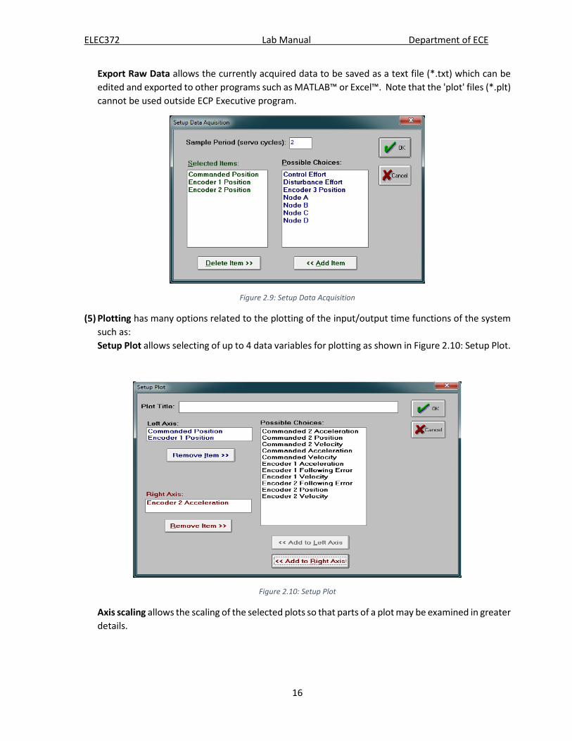
Export Raw Data allows the currently acquired data to be saved as a text file (*.txt) which can be edited and exported to other programs such as MATLAB™ or Excel™. Note that the 'plot' files (*.plt) cannot be used outside ECP Executive program.
Figure 2.9: Setup Data Acquisition
(5) Plotting has many options related to the plotting of the input/output time functions of the system such as: Setup Plot allows selecting of up to 4 data variables for plotting as shown in Figure 2.10: Setup Plot.
Figure 2.10: Setup Plot
Axis scaling allows the scaling of the selected plots so that parts of a plot may be examined in greater details.

ELEC372 Lab Manual Department of ECE
17
Also, Print data loads plot data and prints data to a local printer if connected, and loads a saved plot file into the program, save plot data saves a plot data as a *.plt file which can only be internally used in ECP program.
(6) Utility has six options of which Configure Auxiliary DACs and Rephrase Motor are not applicable to the laboratory system. Download Controller Personality File is a maintenance/service item which is not to be used. Jog Position allows moving the turntables to a different commanded position. Zero Position resets the current position to zero. The Reset Controller option is very useful since it allows the controller to be reset after the loop has been opened due to an overload.
2.6 DATA FOR LAB REPORTS
2.6.1 PLOT FILE Although not mentioned in the procedures, the displayed output plots should be included in your reports. Please note that the ‘PLOT’ files (*.plt) can only be used within ECP32 program. In order to allow students to incorporate the ‘onscreen’ experimental plots obtained in their reports, a screen capture utility called “Smartision Screen Capture” (SSC) is available on the computers. Its ‘shortcut’ can be seen on the desktop. The utility allows capturing and saving the displayed screen preferably as a *.jpg file which can be copied to a USB key, for subsequent use in preparing the lab report.
To obtain plots for your reports use the following procedure:
(1) With the desktop displayed, double click the SSC icon to open the program and its window and then close the window. An SSC icon should appear on the bottom right toolbar. This step is necessary since access to this icon (which will otherwise be hidden under ECP screen) will be required during each experiment.
(2) With the plot sized to ‘full screen’, double click on the above mentioned toolbar SSC icon. This will open the SSC window. Click on <shoot>. The screen will then be displayed within the SSC window. Use the SSC ‘file’ menu to ‘save’ the shot, after naming it, as a *.jpg file. The SSC files should be saved into the ‘my documents’ folder or directly on the desktop or in the USB key directly.
(3) After recording your data, delete all files that you created on the desktop or in the “my documents” folder; do not leave your data files stored on the lab computer.
2.6.2 SAVE DATA 1) Save data on your own USB key; 2) Save data to your ENCS drives.
A. Mount ENCS drives. Click the icon of ‘Map ENCS Drives’, the system shall run a script to map your ENCS network drives G: and U:. The log-in pop-up window is shown below:

ELEC372 Lab Manual Department of ECE
18
Please use your ENCS account to log-on ENCS servers. For detailed information about these two network drives please refer to ENCS helpdesk webpage.
B. Use WinSCP directly. Click the icon of “WinSCP” on the desktop, input ‘login.encs.concordia.ca’ with your ENCS username, then click Login. A pop-up window is shown as the followed:
2.7 SAFETY PROCEDURES The Model ECP220 has the potential of causing physical injury if certain precautions are not followed. It is therefore important to read the regulations and procedures given below and make sure that they are obeyed at all times!
Follow the proper startup and shutdown procedures. Never ‘run’ the system without its plexiglass protective cover in place. Make sure that fingers, hair and loose items of clothes do not come into contact with the belts
or with the turntables at all times. If you notice that any of the brass weights and/or belts are loose, report it immediately to the
instructor. Do not attempt to make any changes or adjustment to the mechanism. If you see or hear the mechanism straining or making unusual sounds, immediately press the
‘red’ abort button on the control box and examine your parameter settings. Do not ‘run’ the mechanism continuously for long periods (i.e. keep the cycling periods small).

ELEC372 Lab Manual Department of ECE
19
3 EXPT #1: FAMILIARIZATION WITH EXPERIMENT SYSTEMS
3.1 OBJECTIVE - To become familiar with the lab equipment (ECP Model 220 system), software and the
procedure to obtain typical system responses. - To use MATLAB in control system application.
3.2 INTRODUCTION
3.2.1 ECP EXECUTIVE CONTROL PROGRAM Please read Section 2 – “LABORATORY EQUIPMENT OVERVIEW” for a detailed introduction.
3.2.2 Open-loop and Closed-loop Block Diagrams In this experiment, you will obtain open-loop and closed-loop responses of the position control system. First we present the block diagrams and transfer functions of the open-loop and closed-loop systems.
Open-loop Block Diagram
The basic ‘rigid’ plant used in the lab system is equivalent to a rotational mass (total inertia of the turntable/motor system, J (kg.m2)) supported by bearings (assumed as ‘viscous friction’ B, N.ms/radian), driven by a servo DC motor.
Figure 3.1: DC Motor Open-loop Diagram
θθ BJVKK iat += (3.1)
• Kt – torque constant • Ka – trans-conductance gain • J – total inertial of turntable system • B - Viscous friction
From (3.1), the transfer function of the DC motor is:
)()()()(
sJBsK
sJBsKK
sVs mta
i +=
+=
θ (3.2)
The angular position is measured using an encoder with the gain eK , thus the overall transfer function
for open-loop test is
ELEC372 Lab Manual Department of ECE
20
)1()()()(
)()(
ssK
sJBsKK
sJBsKKK
sVs
sG oemeta
i
op τ
θ+
=+
=+
== (3.3)
Where 𝐾𝐾0 = 𝐾𝐾𝑎𝑎𝐾𝐾𝑡𝑡 eK 𝐵𝐵⁄ (counts/sec per volt) and 𝜏𝜏 = 𝐽𝐽𝐵𝐵 (sec). From Equation (3.3), we obtain the
angular velocity (counts/sec) as:
𝜔𝜔(𝑠𝑠) = 𝐾𝐾0𝑉𝑉𝑖𝑖(𝑠𝑠)1+𝑠𝑠𝑠𝑠
(3.4)
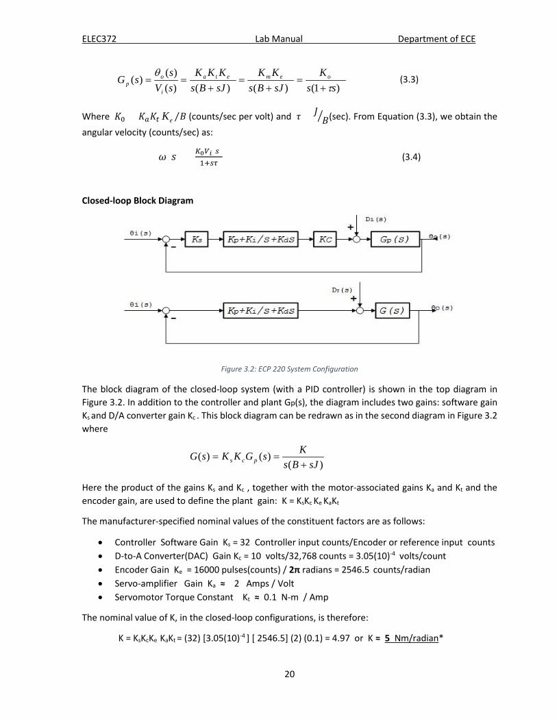
Closed-loop Block Diagram
Figure 3.2: ECP 220 System Configuration
The block diagram of the closed-loop system (with a PID controller) is shown in the top diagram in Figure 3.2. In addition to the controller and plant Gp(s), the diagram includes two gains: software gain Ks and D/A converter gain Kc . This block diagram can be redrawn as in the second diagram in Figure 3.2 where
)(
)()(sJBs
KsGKKsG pcs +==
Here the product of the gains Ks and Kc , together with the motor-associated gains Ka and Kt and the encoder gain, are used to define the plant gain: K = KsKc Ke KaKt
The manufacturer-specified nominal values of the constituent factors are as follows:
• Controller Software Gain Ks = 32 Controller input counts/Encoder or reference input counts • D-to-A Converter(DAC) Gain Kc = 10 volts/32,768 counts = 3.05(10)-4 volts/count • Encoder Gain Ke = 16000 pulses(counts) / 2π radians = 2546.5 counts/radian • Servo-amplifier Gain Ka ≈ 2 Amps / Volt • Servomotor Torque Constant Kt ≈ 0.1 N-m / Amp
The nominal value of K, in the closed-loop configurations, is therefore:
K = KsKcKe KaKt = (32) [3.05(10)-4 ] [ 2546.5] (2) (0.1) = 4.97 or K ≈ 5 Nm/radian*
ELEC372 Lab Manual Department of ECE
21
The nominal values of B and J will be discussed in Experiment #2.
3.2.3 MATLAB 1. MATLAB
MATLAB® is a high-level language and interactive environment for numerical computation, visualization, and programming. Using MATLAB, you can analyze data, develop algorithms, and create models and applications. You can use MATLAB for the applications of control systems, testing, and measurement. MATLAB is widely used in control system analysis, design, and simulation.
2. CONTROL TOOLBOX
Control System Toolbox™ provides industry-standard algorithms and apps for systematically analyzing, designing, and tuning linear control systems. You can specify your system as a transfer function, state-space, pole-zero-gain, or frequency-response model. Apps and functions, such as Step and Bode, let you visualize system behavior in time domain and frequency domain. You can tune compensator parameters using automatic PID controller tuning, Bode loop shaping, root locus method, LQR/LQG design, and other interactive and automated techniques. You can also validate your design by verifying rise time, overshoot, settling time, gain and phase margins, and other requirements.
Useful Functions
• tf - Create transfer function model, convert to transfer function model. • pid - Create PID controller in parallel form, convert to parallel-form PID controller.
References
For more detailed information, please refer to MATLAB Control System toolbox website, http://www.mathworks.com/help/control/index.html
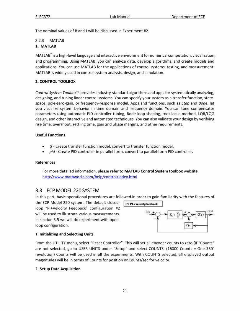
3.3 ECP MODEL 220 SYSTEM In this part, basic operational procedures are followed in order to gain familiarity with the features of the ECP Model 220 system. The default closed-loop “PI+Velocity Feedback” configuration #2 will be used to illustrate various measurements. In section 3.5 we will do experiment with open-loop configuration.
1. Initializing and Selecting Units
From the UTILITY menu, select “Reset Controller”. This will set all encoder counts to zero [If “Counts” are not selected, go to USER UNITS under “Setup” and select COUNTS. (16000 Counts = One 360° revolution) Counts will be used in all the experiments. With COUNTS selected, all displayed output magnitudes will be in terms of Counts for position or Counts/sec for velocity.
2. Setup Data Acquisition

ELEC372 Lab Manual Department of ECE
22
From the DATA menu, select the menu “Setup Data Acquisition” and make sure that Commanded Position and Encoder #1 Position are on the list. Select Sample Period = 2 (This implies that data will be collected every second servo cycle, i.e. at intervals of 2Ts).
3. Setup Control
“Set Up Control Algorithm” window, under which CONTINUOUS TIME, Ts = 0.00442 sec and “PI with Velocity Feedback” have already been selected. Click on SETUP ALGORITHM. This will display the relevant control schematic with the preselected gains Kp =0.2, Kd = 0.01 and Ki = 0. Then click on IMPLEMENT ALGORITHM and OK. This downloads the selected control law to the controller.
Note: ‘Implement’ will always reset the controller unless inconsistent values are set or the loop is opened. The closed-loop system in configuration #2 is now ready for an input command.
4. Choose the system input command
From the COMMAND menu, select “Trajectory” and from the “Trajectory Configuration” window, select STEP (default setting) and then click on “Set Up”. Select CLOSED LOOP. This will display the default Step input parameters: STEP SIZE 4000 Counts, DWELL TIME 1000mS, and Number of Repetitions 1.
5. Execute the command
From the COMMAND menu, select “Execute Trajectory” under which check only NORMAL DATA SAMPLING. Then click on RUN. This will initiate the control action. Wait for the data acquisition to be completed, that is, until the (“Upload Successful 100%”) message appears. Then click OK.
6. Plot the input and output of the step response
From the PLOTTING menu, select “Setup Plot”. Choose for the Left Axis, the variables Commanded Position and Encoder #1 Position. Choose Encoder #1 Following Error for the right axis. Then click on the PLOT DATA button at the lower right hand side of the window. A plot similar to the one shown below should appear.
RESULTS & QUESTIONS
Note how the error varies in the opposite direction of the output and approaches zero in the steady state.
7. Save a copy of the plot for your report
First maximize the display to ‘full screen’ by clicking the ‘maximize’ icon at top right. If you cannot find an icon for the SSC (Smartision screen capture) program on the lower task bar, run it from the desktop. On SSC window, click shoot, then save the image that appears in SSC window as a *.jpg file, on the desktop, after giving it a name. (This image file can be manipulated using Windows Painttm for your report. Among other manipulations, it is most useful to ‘invert colors’, so that the image is saved and printed using a white background, which will not consume large amounts of printer toner or ink). This

ELEC372 Lab Manual Department of ECE
23
procedure for saving plots for your report must be used in all subsequent examples in this experiment as well as in the remaining experiments.
8. Scale the plot for better readability
From the PLOTTING menu -> axis scaling, change the scale of the plots using left/right axis range and horizontal axis.
9. Display the ‘Control Effort’
Repeat Step 2 above to add ‘Control Effort’ (CE) to the list of available variables. Then repeat Step 6 above with the ‘Control Effort’ chosen as the Right Axis variable, instead of the Encoder #1 Error. Then RUN the system with the default step input and then click on the PLOT DATA button.
A plot similar to the one shown below should appear.
RESULTS & QUESTIONS
Note how the CE, which is the input to the servomotor, varies in a manner similar to that of the error, but anticipates the output variation with an observable lead time. The CE is the input whenever the system is operated in the open-loop mode.
3.4 PLOT DATA WITH MATLAB
3.4.1 EXPORT RAW DATA ECP software can export raw data, it allows the currently acquired data to be saved as a text file (*.txt), which can be edited and exported to MATLAB™.
To get raw data, after collecting data:
a. Choose ‘Export Raw Data’ from the Data menu. b. Save your data as a text file in the MATLAB bin folder. Give it a name pertaining to your data,
like “sinesweep220”. c. Using Windows Explorer, change the extension on your file from ‘.txt’ to ‘.m’. d. Open your m-file in MATLAB for editing.
Change the top and bottom of your file like the example below:

ELEC372 Lab Manual Department of ECE
24
The following is a sample code to plot the data. You can copy the sample code into an m-file.
Compare the plots in Matlab with the screenshot on ECP Executive, try to adjust the parameters of the function ‘plot’ to make its output close to ECP format.
3.5 OPEN-LOOP TEST AND SIMULATION In this section we obtain the step response of the open-loop DC motor, first using Matlab simulation then using lab test on the motor. Then we will compare the result.
3.5.1 Matlab Simulation As an example, set the physical constants as:
To see the transfer function:
>>dcm_s >>dcm_p
To see the step response (speed and position) to step voltage input use:
ltiview('step',dcm_s, 0:0.1:10); ltiview('step',dcm_p, 0:0.1:10);
time = data(:,2); %read Time y=data(:,4); %set Encode1 Pos as y u=data(:,6); % Control Effort as input plot(time, y); %Plot data
Ka = 2.0; % Trans-conductance gain Kt = 0.1; % Torque constant Ke = 2546.5; % Encoder gain B = 0.002; % Viscous (N.m.s/rad) J = 0.0043; % kg.m^2 s = tf('s'); dcm_s = Ka*Kt*Ke/(J*s+B); % Speed (counts/s) dcm_p = dcm_s/s; % Position (counts)

ELEC372 Lab Manual Department of ECE
25
Then you can see a similar display as follows:
Also, with right-click on the plot, click "Plot Types”, you can change the input types.
3.5.2 VERIFICATION ON THE EQUIPMENT Now we obtain the step response of the open-loop system.
1. Run ECP program. Under ‘Data Acquisition’ menu, make sure that Control Effort (CE) has been added to the list. Set up the 'plot' to display the Encoder #1 Position on the left axis and the CE on the right axis.
2. Reset the controller from the Utility menu. From the Control Algorithm menu, implement the PID with the following settings:
Ts = 0.00442 sec, Kp = 1 Ki = 0 and Kd = 0.0
3. Obtain the open-loop step response. From the COMMAND menu, select “Trajectory” and from the “Trajectory Configuration” window, select STEP (default setting) and then click on “Set Up”. Select OPEN LOOP: Step Size of 0.4v, Dwell Time of 5000 ms, and number of Repetitions 1.
4. Go to ‘Execute’ to run the test, and display the plot. Use axis-scaling to display only the section of the response within the dwell period of 5 seconds to make the display appear as a ‘step response’. Note that instead of unit step input 1.0v used in simulation, we used 0.4v input to avoid exceeding the motor speed safety limits.
4. Compare the obtained results with the one from 3.5.1.

ELEC372 Lab Manual Department of ECE
26

ELEC372 Lab Manual Department of ECE
27
4 EXPT #2: SYSTEM IDENTIFICATION
4.1 OBJECTIVE - To determine the parameters (J, B and K) of a mechanical first-order system and calculate the
system model. - To illustrates the basic principles of system identification using open-loop and closed-loop
response. - To verify the system modeling by using MATLAB functions.
4.2 INTRODUCTION
4.2.1 SYSTEM PARAMETERS ECP 220 system has the general block diagram shown in Figure 4.1 again, in which, the PI+V controller has been chosen as an example.
Figure 4.1: A closed-loop configuration
In the above closed-loop configurations, the nominal value of forward-path gain K is discussed in Experiment #1:
K = KsKcKe KaKt = (32) [3.05(10)-4 ] (2) (0.1)[ 2546.5] ≈ 5 Nm/radian*
*Notes: The values of Ka and Kt vary from unit to unit and the variation in the actual value of K is ± 20%
The actual values of J and K specific to each unit will be found in this Experiment. The “PI + velocity feedback” configuration (see Figure 4.1 above), which is also the ‘default’ configuration, will be used since it allows good control of closed-loop system parameters.
4.2.2 THEORETICAL ESTIMATION OF ROTATIONAL INERTIA J Since the feedback loop is closed around Encoder #1 in the laboratory system, the J and B in the system equations must be values ‘reflected’ to the location of encoder #1. The arrangement of the belt and pulley coupling between the disks and the drive motor (shown earlier in this manual) is shown schematically in Figure 4.2: Plan Rotation Inertia. Assuming ‘ideal coupler’ or ‘transformer’ relations, it can be shown that for gears or for toothed-belt and pulleys, the coupling ratio is n = ωp/ω s = θp/θ s = Νs/Νp where N is the number of teeth and ‘p’ and ‘s’ refer to primary (driving side) and secondary (driven side). Thus, in fowling Figure 4.2, the overall coupling-ratio is n = ω1/ω2 = θ1/θ2 = n1n2 = [Nbottom/ND] [NL/Ntop] = (24/12) (72/36)=(2)(2)=4. Furthermore, an inertia J or friction B on the secondary side will appear to the primary-side as being multiplied by (1/n2). Thus, the total effective inertia at the Encoder#1 location can be expressed as:

ELEC372 Lab Manual Department of ECE
28
Toothed Belts
LOAD DISK
DRIVE DISK
SR ASS’Y PULLEYS
NL= 72ND= 12
NTop= 36NBottom= 24
ENCODER#1
ENCODER#2
θ2
θ1
Note: The 1:1 coupling between the Drive Disk and Drive Motor & the 4:1 coupling between the Distrurbance Motor and the Load Disk are not
shown.Also the disk diameters and spacing are not to scale.
Figure 4.2: Plan Rotation Inertia
𝐽𝐽 = (𝐽𝐽𝐷𝐷 + 𝐽𝐽𝑊𝑊𝐷𝐷) + 𝐽𝐽𝑆𝑆𝑆𝑆(𝑛𝑛1)2
+ 𝐽𝐽𝐿𝐿+𝐽𝐽𝑊𝑊𝐿𝐿(𝑛𝑛1𝑛𝑛2)2
(4.3)
where the subscripts D, L and SR refer to the drive, the load and the SR disks and the additional subscript w refers to the additional inertia provide by the weights fixed to the drive and load disks. The inertias𝐽𝐽𝐷𝐷, 𝐽𝐽𝐿𝐿, and 𝐽𝐽𝑆𝑆𝑆𝑆 are specified by the manufacturer as:
• Inertia of the bare drive disk 𝐽𝐽𝐷𝐷 = 4(10)-4 kgm2
• Inertia of the bare load disk 𝐽𝐽𝐿𝐿 = 65(10)-4 kgm2
• Inertia of the SR assembly 𝐽𝐽𝑆𝑆𝑆𝑆 = 78(10)-6kgm2
(Including top and bottom pulleys, backlash device and screws)
The inertias JwD and JwL must now be calculated: The nominal mass (m) values of the small and larger [diameters 32mm and 50mm respectively] brass weights are 200gm and 500gm respectively. When symmetrically located at a radius R on the disks, their moment of inertia can be calculated as Jw = mR2
at the appropriate location. It is assumed that the small and large weights will be used on the drive and load disks respectively. Further, it is assumed that four identical weights will be used symmetrically on each disk. Since the nominal radii of the drive and load disks are 67mm and 128mm respectively, the radius can be deduced with reasonable accuracy when the masses are moved outwards so that their outside edges are flush with the outside edges of the disks, as seen in Figure 2.2: Rotational-motion Assembly of this manual. With the weights permanently bolted at the extremes as explained, the inertia values JwD and JwL are:
JwD = 4 (0.2) [0.067 – 0.016]2 = 2.08(10)-3 kgm2
and JwL = 4 (0.5) [0.128 – 0.025]2 = 2.122(10)-2 kgm2
Equation (3.5) can now be used to calculate the total effective inertia J at the Encoder#1 location as:
J = ( JD + JwD) + JSR/ (n1)2 + (JL + JwL)/( n1 n1)2
= 4(10)-4 + 2.08(10)-3 + (78/4)(10)-6 + [65(10)-4 + 2.122(10)-2 ]/16
= 4.23(10)-3 kgm2.

ELEC372 Lab Manual Department of ECE
29
Note that the largest contribution to J is made by the added brass weights. Also note that the value of J will vary somewhat from unit to unit.
4.2.3 MATLAB IDENTIFICATION TOOLBOX System Identification Toolbox™ provides MATLAB® functions, Simulink® blocks, and an app for constructing mathematical models of dynamic systems from measured input-output data. It lets you create and use models of dynamic systems not easily modeled from first principles or specifications. You can use time-domain and frequency-domain input-output data to identify continuous-time and discrete-time transfer functions, process models, and state-space models. More information, please visit its website.
Useful Function tfest - Transfer function estimation and the System Identification Tool GUI - ident.
4.3 PLANT PARAMETER AND SYSTEM MODELING In this experiment, open-loop tests are performed on the DC motor (plant) to obtain parameters of its transfer function, since the transfer function of the plant is required for analysis of the closed-loop system.
4.3.1 EVALUATION OF J AND K USING OPEN-LOOP VELOCITY OUTPUT
PRELIMINARY In this experiment, the acceleration α1 developed in response to a step voltage Vi is measured. Next, the inertia is increased by a known amount ∆J and the acceleration α2 developed in response to the same step voltage is measured. The step magnitude is selected to provide rapid observable acceleration so that the friction torque may be neglected and the torque equation T ≈ J α may be used. Since only the partial gain product KaKtKe is involved, we have:
(Vi) KaKtKe = J α1 = (J + ∆J) α2 (4.7)
Where the acceleration α is expressed in counts/sec2 and α1> α2. If ∆J is known (as it is, see Step 4 in the Procedure below), J can be determined from the equation
JJ21
2 ∆
α−αα
= kgm2 (4.8)
PROCEDURE:
1) Reset the controller from the UTILITY menu. Set up the ‘plot’ to display Encoder #1 Velocity only on the left axis. Under ‘Data Acquisition’ menu, set the sampling period to 5 (ie data to be collected every 5th cycle, = 5 (4.42 ms) ≈ 22ms which is done to reduce the noise inherent in acquiring the velocity signal).
2) From the COMMAND menu, select ‘Trajectory’, STEP and then click on ‘Setup’. Then select OPEN LOOP, Step Size 2 volts, Dwell time 500 ms, and number of Repetitions 1. Next, go to Execute and RUN the test. After the data has been acquired, plot the output. The trace will be similar to the one shown below. (The initial linear part of the curve denotes constant acceleration). Overload occurs

ELEC372 Lab Manual Department of ECE
30
at approximately 0.5 sec when the step reverses and the ‘overload’ circuit will disable the system at this point.
3) Determine* the slope of the initial linear part of the velocity plot, without using any axis scaling. This is the acceleration α1 in Counts /sec2 which results in response to the step input voltage Vi = 2 volts. (*Read the note at the beginning of the experiment about making preliminary calculations)
4) Making sure that the system is still disabled, loosen the cover screws and lift off the plexiglass cover. Carefully insert the additional 69mm diameter brass weight (supplied) in between the four fixed 0.2 kg weights on the drive disk so that it fits in snugly. Make sure that the pins on the weight fit into the radial slots on the disk, and then carefully replace the plexiglass cover. (Note: The extra weight added has been calculated to increase the net inertia effective at the drive disk axis by the amount ∆J ≈ 0.000494 kg.m2 for all stations)
5) Repeat Steps 1, 2, and 3 above with the extra weight installed. Determine the acceleration obtained with the added weight in place, as α2 (Note that α2 < α1). Finally, switch off the controller box, remove the added weight, replace the cover and lightly re-tighten the cover screws. Two typical open-loop velocity responses obtained, without and with the added weight are seen in the photograph shown below, in ‘background’ and ‘foreground’ traces respectively.
RESULTS
Using Equation (4.8), determine the value of J and compare the value obtained with the calculated nominal value given in sections (4.2.1) and (4.2.2) and find the % error.
Using the determined value of J, find KaKtKe from the equation 2KaKtKe = Jα1 Multiply this value by KsKc to obtain K (see section 4.2.1) for the equipment at your lab station.
From data given in introduction,
KsKc =(10/32768) (32) ≈ 0.009766 Volts/count.
Record the determined values of J and K found in this part of the experiment.
4.3.2 EVALUATION OF J AND K USING OPEN-LOOP POSITION OUTPUT
PRELIMINARY

ELEC372 Lab Manual Department of ECE
31
The time responses, ω(t), and θ(t) of the system are readily obtained by finding the inverse Laplace transforms of ω(s) and θο(s), respectively, for any given Vi(s). For a step voltage magnitude of A volts, Vi(s) = A/s, after performing the inverse transformation we obtain:
ω(t) = L-1 Ko A/s(1+ sτ) = Ko A[ 1- e –t/τ ]
and θο(t) = L-1 KoA / s2(1+ sτ) = KoA [t − τ + τe –t/τ ] (4.9)
where Ko= KaKt/B. These two step responses are shown below, in normalized form, (ω/KoA) and (θο /KoA) in following figures (a) and (b) respectively.
1ω/KoA
tτ
Normalized velocity
t
0.632
0
θ/KoANormalized position
0
Linear approximation for t >> τ
(a) (b)τ
For the angular velocity output, the response is of the classic ‘rising exponential type with ω(t) approaching KoA for large t and the response reaching 0.632 KoA at t = τ. For the angular position output in equation (3.5.1), a linear approximation may be made by drawing a tangent to the curve for large t: This tangent will intersect the time axis (θ = 0) at t = τ. The slope of the tangent is KoA (radians/sec). The latter response will be used in Experiment #2 to evaluate the ‘plant’ parameters in the laboratory system.
In this test, a smaller step voltage Vi is used as input and the position output is measured. Attempting to use an input that appears as a ‘step’, however, will trigger the built-in ‘overload’ circuit which will automatically ‘abort’ the test. Therefore, a small magnitude ‘bounded’ step is used which will tend to make the output ‘converge’ to a finite value, and half of the response time period can then be taken to correspond to Equation (3.8). It is easily seen that a linear approximation of the above response has a slope S given by KoVi (ie = KaKt Ke Vi /B) and the straight-line describing this linear approximation will intercept the x-axis (time-axis) at t = τ = J/B. Thus, measurement of the slope S and the time-axis intercept τ may be used to find both J and B.
PROCEDURE
1) Under ‘Data Acquisition’ menu, make sure that Control Effort (CE) has been added to the list. Reset the controller from the UTILITY menu. Set up the 'plot' to display the Encoder #1 Position on the left axis and the CE on the right axis.
2) From the COMMAND menu, select ‘Trajectory’, STEP and then click on ‘Set Up’. Then select OPEN LOOP, Step Size 0.5 volts, Dwell time 5000 ms, and number of repetitions 1. Next, go to “Execute” and RUN the test. After the data has been acquired, plot the output. The trace will be similar to the one shown below. (The first half of the response, 0 to 5 sec, is due to the positive step). Of course, the slope and intercept values will have some variation depending upon the station equipment.

ELEC372 Lab Manual Department of ECE
32
The straight line approximation (the line is tangential to the S-shaped curve at midpoint, approx. 5sec.) has been inserted in the plot shown below. Determine* the slope S of the line (in Counts/sec) and the time-axis intercept τ (sec).
RESULTS:
From the displayed slope S (in counts/sec), determine*
S (radians/sec) = S (counts/sec) / Ke
= S (counts/sec) / 2546.5 = 3.927(10)-4 S (counts/sec)
Since Vi = 0.5 volt, S (radians/sec) = KaKtVi /B= (2) (0.1) (0.5)/B
Hence, determine
B (Nms/radian) = sec)/(
1.0radiansS
= sec)/counts(S
65.256
From the displayed time-axis intercept, determine the time-constant τ = J/B from x-axis intercept. Finally determine J:
J(kg.m2) = Bτ
Record the determined values of J and B found in this part of the experiment. Compare the value of J found with the value determined in section 4.3.1 and obtain the average value. Compare the average value of J with the calculated nominal value given in section 4.2.2 and find the percentage error.
Record the average value of J, and the values of B and K obtained, these values are to be used in subsequent lab work.
4.3.3 SYSTEM IDENTIFICATION VIA THE OPEN-LOOP RESPONSE TO A SINE SWEEP INPUT The system position output θo(s) is given by Equation 3.2, shown the Figure 4.3. Αs mentioned in the description of the system, selecting ‘open loop’ under the Trajectory Setup menu allows a voltage input to be applied to the plant. Among the inputs, the step and sinusoidal inputs are available for open-loop tests.

ELEC372 Lab Manual Department of ECE
33
Here sinusoidal signal is chosen to evaluate the system parameters.
1) Set up the controller. Under the Set-up menu, set Ts=0.00442sec and select Continuous Time Control. Select PI With Velocity Feedback and Set-up Algorithm. Enter the kp = 1 and kd = 0, ki = 0 and select Implement Algorithm, then OK.
2) Under Setup Plot, choose the Control effort (CE) to be displayed on the Left axis and Encoder#1 Velocity to be displayed on the Right axis (If the CE is not available, it should be added to the list using the Data Acquisition setup menu).
3) From Trajectory, choose sinusoidal linear sweep input of 0.1 to 12 Hz, 0.5 volt, and sweep time of 30 sec, and choose Open Loop mode, choose Open Loop mode. Then RUN the system. A plot similar to the one seen below should result.
4) Export raw data to a file. From the menu DATA, choose “Export Raw Data”, name the data file, e.g.
raw_data_freq.txt, and then you can transfer data file to MATLAB. More details to see part 2.6.2. Modify the raw data file raw_data_freq.txt to a MATLAB m-file separately.
5) Load it into MATLAB workspace. Try to use the functions, e.g. ‘iddata’, ‘tfest’ of MATLAB System Identification Toolbox, to obtain DC motor first order and second-order transform functions.
RESULTS
Compare the results from MATLAB and the model obtained from experiment.
4.3.4 SYSTEM IDENTIFICATION VIA CLOSED-LOOP SYSTEM RESPONSE
PRELIMINARY In the Figure 4.1, 𝐺𝐺(𝑠𝑠) = 𝐾𝐾
𝑠𝑠(𝐵𝐵+𝐽𝐽𝑠𝑠), set Ki=0, then the closed-loop transfer function (CLTF) will be:
>> time = data(:,2); %read Time >> y=data(:,4); %set Encode1 Pos as y >> u=data(:,6); % Control Effort as input >> dy= diff(y); %We need speed as Output >> dy(end +1) = dy(end); %restore sector size to N >> zf = iddata(dy,u,0.00884); %set Object iddata >> tf1 = tfest(zf,1,0) ; %for First order

ELEC372 Lab Manual Department of ECE
34
pd
p
KKsKKBJsKK
sT+++
=)(
)( 2 (4.10)
When set Kp =1.0 and Kd=0, the system output will be highly oscillatory. In this case, set a value, e.g. Kd =0.01, just after data acquisition is complete. Click on Plot and view the waveform. If the waveform is good, the raw-data could be save into a file for MATLAB analysis.
Procedure:
1) Set up the controller. Under the Set-up menu and set Ts=0.00442 s and select Continuous Time Control. Select PI With Velocity Feedback and Set-up Algorithm. Enter Kp=1, Kd=0, and Ki=0 and select Implement Algorithm, then OK.
2) Go to Set up Data Acquisition in the Data menu and select encoder #1, Commanded Position as data to acquire and specify data sampling every 2 servo cycles. Select Zero Position from the Utility menu to zero the encoder positions.
3) Under Setup Plot, choose both Commanded Position and Encoder#1 Position to be displayed on the left axis.
4) Enter the Command menu, go to Trajectory and select Step. Select Closed Loop Step and input a step size of 1000 counts, duration of 2000ms and 1 repetition. Select Execute from the Command menu and select Run. The drive disk will step, oscillate, and attenuate, then return. Encoder data is collected to record this response. Select OK after data is uploaded.
5) Click on Plot and view the waveform. If the data is not satisfactory, repeat the above steps or modify Kp and Kd if necessary.
6) Export raw data to a file. From the menu DATA, choose “Export Raw Data”, name the data file, e.g. raw_data_cl_step1.txt, then you can transfer data file to MATLAB. See the section 2.6.2 for details.
7) Enter the Control Algorithm box, enter the Kp = 1 and Kd = 0.01, Ki = 0 and run steps 4-6 again, save another data file.
8) Convert the raw data files, raw_data_cl_step1.txt and raw_data_step2.txt, to a MATLAB m-files. 9) Load it into MATLAB workspace. Try to use the functions of MATLAB System Identification Toolbox,
such as ‘iddata’, ‘tfest’, to obtain the second-order transfer functions of the closed-loop system and then the DC motor first-order transfer function G(s).
>> time = data(:,2); %read Time >> y=data(:,4); %set Encode1 Pos as y >> u=data(:,3); % Control Position as input >> zf = iddata(y,u,0.00884); %set Object iddata >> Tfd2 = tfest(zf,2,0); % for second order

ELEC372 Lab Manual Department of ECE
35
RESULTS
1) Calculate system the open-loop transfer function (OLTF) with the determined values of K, J and B from open-loop tests in section 4.3.2 and 4.3.3.
2) Obtain the OLTF in MATLAB by the data of the closed-loop test.
3) Compare these models.
4) Write a brief summary about how the lab equipment might facilitate a better understanding of control systems.
=======================================
ELEC372 Lab Manual Department of ECE
36
5 EXPT #3: IMPROVING SYSTEM PERFORMANCE
5.1 OBJECTIVE - To study how to improve the system performance by PD, PI and PID control. - To learn how to eliminate the steady state error caused by a disturbance input.
5.2 INTRODUCTION
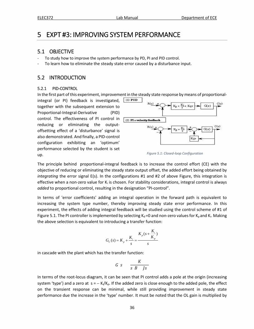
5.2.1 PID-CONTROL In the first part of this experiment, improvement in the steady state response by means of proportional-integral (or PI) feedback is investigated, together with the subsequent extension to Proportional-Integral-Derivative (PID) control. The effectiveness of PI control in reducing or eliminating the output-offsetting effect of a ‘disturbance’ signal is also demonstrated. And finally, a PID-control configuration exhibiting an ‘optimum’ performance selected by the student is set up.
The principle behind proportional-integral feedback is to increase the control effort (CE) with the objective of reducing or eliminating the steady state output offset, the added effort being obtained by integrating the error signal E(s). In the configurations #1 and #2 of above Figure, this integration is effective when a non-zero value for Ki is chosen. For stability considerations, integral control is always added to proportional control, resulting in the designation “PI-control”.
In terms of 'error coefficients' adding an integral operation in the forward path is equivalent to increasing the system type number, thereby improving steady state error performance. In this experiment, the effects of adding integral feedback will be studied using the control scheme of #1 of Figure 5.1. The PI controller is implemented by selecting Kd =0 and non-zero values for Kp and Ki. Making the above selection is equivalent to introducing a transfer function:
( )( )
ip
piC p
KK sKK
G s Ks s
+
= + =
in cascade with the plant which has the transfer function:
𝐺𝐺(𝑠𝑠) =𝐾𝐾
𝑠𝑠(𝐵𝐵 + 𝐽𝐽𝑠𝑠)
In terms of the root-locus diagram, it can be seen that PI control adds a pole at the origin (increasing system ‘type’) and a zero at s = − Ki/Kp. If the added zero is close enough to the added pole, the effect on the transient response can be minimal, while still providing improvement in steady state performance due the increase in the ‘type’ number. It must be noted that the OL gain is multiplied by
Figure 5.1: Closed-loop Configuration

ELEC372 Lab Manual Department of ECE
37
Kp and a gain adjustment may be necessary. Considering the unity feedback system (UFS) OLTF of GcGp , however, it can be seen that the addition of integral control will also increase the system order. The increase in system order has the tendency of degrading the relative stability of the system which may be observed, for example, as an increase in the overshoot. This disadvantage can be overcome by introducing ‘derivative control’, thereby leading to what is known as “PID-control” (or “Three-Mode” control). For a PID controller, the transfer function is
2[ ]( )
p i
i d dC p d d
K Ks sK K K
G s K K s Ks s
+ += + + =
In terms of the root-locus diagram, a pole is introduced at the origin increasing the system ‘type number’ as before, and two finite zeros are introduced. The two zeros may be located on the real axis or may be complex conjugates in the ‘left-half-plane’. (It can be shown that the latter condition will result if Kp
< 2 diKK ). While the increase in system type improves the steady state error performance, the
attendant degradation in relative stability is counteracted by the presence of the finite zeros in the ‘left-half-plane’. PID control is commonly used in industrial control systems, the adjustment process for the three coefficients being called a “tuning” operation. Rather than determining the required settings analytically, various semi-empirical and well-established tuning procedures (such as the “Ziegler-Nichols tuning rules”) are used in practice (See your course textbook for further information about this topic).
STEADY STATE ERROR
The ‘error’ 𝑒𝑒(𝑡𝑡) is defined as the difference between the command input 𝑟𝑟(𝑡𝑡) and the output 𝑐𝑐(𝑡𝑡) ; i.e. 𝑒𝑒(𝑡𝑡) = 𝑟𝑟(𝑡𝑡) −𝑐𝑐(𝑡𝑡). The steady state or ‘static’ error (𝑒𝑒𝑠𝑠𝑠𝑠) is the final value of 𝑒𝑒(𝑡𝑡) that is reached as time t approaches infinity, i.e. 𝑒𝑒(∞). In the frequncy domain, the “Final Value Theorem” (FVT) can be used to obtain 𝑒𝑒𝑠𝑠𝑠𝑠:
𝑒𝑒𝑠𝑠𝑠𝑠 = 𝑒𝑒(∞) = lim𝑠𝑠→0
𝑠𝑠𝑠𝑠(𝑠𝑠)
For a unity feedback system (UFS) in Figure 5.2, assuming it is stable, we have
𝑠𝑠(𝑠𝑠) = 𝑅𝑅(𝑠𝑠)− 𝑅𝑅(𝑠𝑠)𝑇𝑇(𝑠𝑠) = 𝑅𝑅(𝑠𝑠) 1 − 𝐺𝐺(𝑠𝑠)1+𝐺𝐺(𝑠𝑠) = 𝑅𝑅(𝑠𝑠) 1
1+𝐺𝐺(𝑠𝑠) (5.1)
where 𝐺𝐺(𝑠𝑠)the transfer is function of the system and 𝑅𝑅(𝑠𝑠) is the input. 𝑒𝑒𝑠𝑠𝑠𝑠 can result in values of zero, a finite number, or ∞. For a given input, 𝑒𝑒𝑠𝑠𝑠𝑠 depends on the form of 𝐺𝐺(𝑠𝑠), especially on the presence and number of 𝑠𝑠 terms in the denominator of 𝐺𝐺(𝑠𝑠) (i.e. the poles of 𝐺𝐺(𝑠𝑠) at the origin). For this reason, systems are classified in terms of the number of poles of the OLTF at the origin, which is called the system “Type number” (𝑁𝑁). Thus, 𝑒𝑒𝑠𝑠𝑠𝑠 depends on both 𝑁𝑁 and 𝑅𝑅(𝑠𝑠).
For example, consider the UFS OLTF 𝐺𝐺(𝑠𝑠) = 10 𝑠𝑠(𝑠𝑠 + 2)⁄ . The system Type is 1 since there is one 𝑠𝑠 term in the denominator of the OLTF. However, the order of this system is 2 since it has two poles. Now consider unit step (𝑅𝑅(𝑠𝑠) = 1 𝑠𝑠⁄ ) and unit ramp (𝑅𝑅(𝑠𝑠) = 1 𝑠𝑠2⁄ ) inputs to the closed-loop system which has this OLTF.
Figure 5.2: Unity Feedback System

ELEC372 Lab Manual Department of ECE
38
For the step input,
𝑒𝑒𝑠𝑠𝑠𝑠 = lim𝑠𝑠→0
𝑠𝑠(1𝑠𝑠)( 11+ 10
𝑠𝑠(𝑠𝑠+2)) = 1
1+∞= 0 (i.e. zero error)
For the ramp input,
𝑒𝑒𝑠𝑠𝑠𝑠 = lim𝑠𝑠→0
𝑠𝑠( 1𝑠𝑠2
)( 11+ 10
𝑠𝑠(𝑠𝑠+2)) = lim
𝑠𝑠→0 ( (𝑠𝑠+2)𝑠𝑠(𝑠𝑠+2)+10
) = 210
= 0.2 (i.e. a finite error)
If the input is extended to a unit parabolic function 𝑟𝑟(𝑡𝑡) = 𝑡𝑡2 2⁄ (𝑅𝑅(𝑠𝑠) = 1 𝑠𝑠3⁄ ) and the application of the FVT as above will yield a 𝑒𝑒𝑠𝑠𝑠𝑠 = ∞ i.e. a Type 1 system will have zero error for step inputs, a finite error for ramp inputs and infinite error for parabolic inputs. Static error analyses, such as the above, can be standardized by expressing 𝑒𝑒𝑠𝑠𝑠𝑠 in terms of “error coefficients” (or error constants) 𝑘𝑘𝑗𝑗 defined as follows:
(General) Error coefficient 𝑘𝑘𝑗𝑗 = lim𝑠𝑠→0
𝑠𝑠𝑗𝑗𝐺𝐺(𝑠𝑠) where 𝑗𝑗 = 0,1,2, … (5.2)
Following historical terminology used for early positional servomechanisms, the error coefficients corresponding to 𝑗𝑗 = 0,1, and 2 are called the positional, velocity and acceleration error coefficients respectively. These are designated in this manual as 𝑘𝑘𝑝𝑝𝑝𝑝𝑠𝑠 , 𝑘𝑘𝑣𝑣𝑣𝑣𝑣𝑣 , and 𝑘𝑘𝑎𝑎𝑎𝑎𝑎𝑎 respectively, in order to avoid possible confusion with variables such as 𝑘𝑘𝑝𝑝 used elsewhere in the manual. The three constants could alternatively be called the step, ramp and parabolic error coefficients. Thus
𝑘𝑘𝑝𝑝𝑝𝑝𝑠𝑠 = lim𝑠𝑠→0
𝑠𝑠0𝐺𝐺(𝑠𝑠) = 𝐺𝐺(0) and 𝑒𝑒𝑠𝑠𝑠𝑠(𝑠𝑠𝑡𝑡𝑒𝑒𝑠𝑠) = 11+𝑘𝑘𝑝𝑝𝑝𝑝𝑠𝑠
𝑘𝑘𝑣𝑣𝑣𝑣𝑣𝑣 = lim𝑠𝑠→0
𝑠𝑠1𝐺𝐺(𝑠𝑠) and 𝑒𝑒𝑠𝑠𝑠𝑠(𝑟𝑟𝑟𝑟𝑟𝑟𝑠𝑠) = 1𝑘𝑘𝑣𝑣𝑣𝑣𝑣𝑣
(5.3)
𝑘𝑘𝑎𝑎𝑎𝑎𝑎𝑎 = lim𝑠𝑠→0
𝑠𝑠2𝐺𝐺(𝑠𝑠) and 𝑒𝑒𝑠𝑠𝑠𝑠(𝑠𝑠𝑟𝑟𝑟𝑟𝑟𝑟𝑝𝑝𝑝𝑝𝑝𝑝𝑝𝑝𝑐𝑐) = 1𝑘𝑘𝑎𝑎𝑎𝑎𝑎𝑎
The error shown is for a unit input and must be multiplied by the magnitude A of the actual input used. Steady state error can be expressed as the absolute value or as a percent of the input magnitude. In the latter case, the unit magnitude given by Equations (5.2) is in fact the decimal value of the percent figure. A table giving 𝑒𝑒𝑠𝑠𝑠𝑠 for the three different inputs as a function of system Type N is shown in table 5.1.
The above results indicate that:
(1) to follow a step input with finite error, at least a Type 0 system is required (2) to follow a ramp input with finite error, at least a Type 1 system is required (3) to follow a parabolic input with finite error, at least a Type 2 system is required
Also, it is worth mentioning that whenever a finite error results, its value will depend on 𝑘𝑘𝑗𝑗 which in turn is dependent upon the system parameters such as the gain. In many cases, an attempt towards extreme minimization of 𝑒𝑒𝑠𝑠𝑠𝑠 by increasing gain, for example, may fail because the system becomes unstable at the selected gain.
Table 5.1. Steady state error for specified input and type number

ELEC372 Lab Manual Department of ECE
39
5.2.2 DISTUTBANCE CONTROL In regulatory systems, the error introduced by a disturbance input d(t) can be reduced to zero by PI control.
Feedback Element(s)
+
DISTURBANCE INPUT D(s)
X(s)+
−
Controller PlantREFERENCE INPUT R(s)
+ CONTROLLED OUTPUT C(s)
H(s)
Gp(s)Gc(s)E(s)
Feedback Signal Y(s)
Figure 5.3: Disturbance control
The response of the closed-loop system to a disturbance D(s) can be investigated by considering D(s) as the input with R(s) set to zero. With R(s)=0, the effective ‘disturbance transfer function’ being given by
TD(s) = )()(
sDsC
= Gp / (1 + Gp Gc H ) = )s(H)s(G1
)s(G p
+
where G(s)=Gp(s)Gc(s). It is seen that a high ‘loop gain’ G(s)H(s) will reduce the effect of the disturbance D(s).
5.3 PID CONTROL
5.3.1 PI - CONTROL The step response of a system with proportional controller is obtained first by setting Ki = Kd = 0 and Kp
to some specific value. Viscous friction (input disturbance) is then introduced through the disturbance motor and its value is increased resulting in steady-state error in step response. Integral feedback is then introduced and its effect of reducing the steady state error is seen.
REMINDER: to use only the continuous domain specifications and procedures, ie under ‘SETUP’, all that is needed is to check the “Continuous Time” button and then “Set Up Algorithm”, and then click on “Implement Algorithm” after setting the controller coefficients.

ELEC372 Lab Manual Department of ECE
40
1) Reset the controller from the Utility menu. From the Set Up Control Algorithm implement the PID configuration (#1 in Figure 2.5) with Ki = Kd = 0 and with Kp = 0.2. Set up a closed-loop step response input using a step size of 4000 Counts, dwell time of 8000 ms. number of repetitions 1. RUN the step test and use axis scaling. A response similar to that shown below will be obtained. Determine* values for the overshoot (using suitable axis scaling of the plot) as well as the damped natural frequency ωd.
2) Next, from the ‘Command’ menu, select ‘Disturbance configuration’, ‘Viscous Friction’ and set it to 4 volt-sec/radian. Then, after checking ‘Implement’ and OK, RUN the step test again. Make sure to check the “Include Viscous friction” box before clicking on ‘RUN’. A step response, similar to the one shown below, should result. The response shows better damping but a finite offset in the steady state. Measure the offset error.
3) Re-implement the controller with Ki set to successive values from 0.02 to 0.1 in steps of 0.02 and RUN the step test at each value. Select and note* the value of Ki which will minimize the steady state error to some acceptable value within 5%. Record* your observations. A typical response with Kp= 0.2, VF = 4 Volt-sec/radian and Ki = 0.03 is shown below.
RESULTS
1) Describe the effect of increase in Ki on the offset error and on the overshoot. 2) Derive the CLTF for the PID system (#1 in Figure 5.1) and obtain the relation between coefficients
required for stability (Note that for a cubic equation
DT(s) = a s3 + b s2 + c s + d = 0,
no root will have a positive real part if the condition 𝑝𝑝 × 𝑐𝑐 > 𝑟𝑟 × 𝑑𝑑 is satisfied)
5.3.2 PID-CONTROL 1) From the Utility menu, reset the controller. Next, from the “Command” menu, remove the viscous
friction and the disturbance input. Implement the PID controller with Kp= 0.2, and Ki = Kd = 0. Obtain the closed-loop step response using a step size of 4000 Counts, dwell time of 4000 ms, number of Repetitions 1. Display the response within the dwell period and reduce the display for later comparison. A typical plot that results from this step is shown below.

ELEC372 Lab Manual Department of ECE
41
2) Successively increase the value of Kd in a small enough step, e.g. 0.002, and set its value so that a desirable overshoot (in your opinion) is obtained. Overshoot values in the 5 ~10% range are generally considered acceptable. An offset error will be noticed. Record the chosen value of Kd , the OS and the steady state error.
3) Next, successively increase the value of Ki in steps of 0.01 until the offset in the step response is almost reduced to zero. Record the chosen value of Ki. Typical displays that result from above Steps and the current one (after setting a suitable values) are shown below. Results Tabulate your choice of controller coefficients for PID control.
Kp=0.2Kd=0.015OS≈7%ess≈1.3%
Kp=0.2Kd=0.015Kd=0.028OS≈8%ess≈ 0
5.4 STEADY STATE ERROR ANALYSIS
5.4.1 USE STEP SIGNAL WITH PD 1) Reset the controller from the Utility menu. From the Set Up Control Algorithm menu implement
the “PI + velocity feedback” with the following settings: Ts = 0.00442s, Kp = 1, Ki = 0 and Kd = 0.01 with Continuous Time type .
2) Perform a closed-loop step test using a Step Size of 4000 Counts, Dwell Time of 4000 ms and Number of Repetitions 1.
3) Observe the output which is highly oscillatory. 4) Click on Plot and view the waveform. Using axis scaling, obtain* the steady state step error (tracking
error) in counts using the increasing part of the response. 5) Repeat above steps with Kp equals 0.5 and 0.2. Keep Ki and Kd unchanged. It will be seen that the
system is now stable and an underdamped step response results. Obtain* the PO and the damped natural frequency ωd using suitable axis scaling. Increase Kd to 0.1 and observe the effect on the step response.

ELEC372 Lab Manual Department of ECE
42
Typical results show the stabilizing effect of increasing Kd are seen in the screen below.
Kp=1, Ki=0PI+V
Kd =0 Kd = 0.01
Kd = 0.1
5.4.2 USE RAMP SIGNAL 1) Reset the controller from the Utility menu. From the Set Up Control Algorithm menu implement
the “PI + velocity feedback” with the following settings: Ts = 0.00442s, Kp = 1, Ki = 0 and Kd = 0 with Continuous Time type.
2) Set up and perform a RAMP test with a Ramp Size of 10000 counts, Velocity 10000 Counts/sec, Dwell Time of 100 ms, number of Repetitions 1 (these are the default values).
3) Observe the output which is highly oscillatory. 4) Click on Plot and view the waveform. Using axis scaling, obtain* the steady state Step error
(tracking error) in counts using the increasing part of the response.
Following or Tracking Error
Expanded display using Axis Scaling to find the tracking error
ess can be readily found from the y-axis intercepts.
5) Repeat Steps 2-4 above using the same gains (Kp= 1, Ki = 0, and Kd= 0.01) but with the “PID” controller (#1 of Figure 2.5) implemented instead of the “PI +Velocity feedback” configuration. Note that in this case, there is no minor loop.
RESULTS

ELEC372 Lab Manual Department of ECE
43
- Tabulate the results of the step and ramp tests for the two different controller implementations. Is there any change in the step response between the two cases? What is the difference in the ramp response between the two cases?
- The equivalent UFS OLTF and the CLTF for the “PI+Velocity feedback” system were already given. for both the systems. Derive the corresponding transfer functions for the system using the “PID” controller with Ki =0. Show that in both cases, the system Type number is 1.
Calculate the ‘velocity-error’ coefficients Kvel for the two cases.
The steady state ramp error is given by: ess(ramp) = Ramp magnitude / Kvel
Hence, for a ramp input of 10,000 Counts/sec,
Kvel = 10000 / ess(Counts/sec)
Show that the velocity error-coefficients for the configurations #1 (PID) and #2 (PI+V) of Figure 5.1 with Ki =0 are respectively
Kvel (PID)= KKp/B and Kvel(PI+V) = KKp/[B+KKd].
Note that Kvel(PID)> Kvel(PI+V) and hence the corresponding steady state ramp error for the PID controller will be the smaller of the two.
5.5 DISTURBANCE ATTENUATION The effectiveness of PI control in eliminating the steady state error caused by a disturbance input will be demonstrated. Please note that the settings given are only typical since gain and inertia and friction vary from unit to unit.
1) Set up a PID control scheme with Continuous Time type, with Kp = 0.2 and Ki = Kd = 0 and with viscous friction introduced though the disturbance motor and set at 4 Volt-sec/radian.
2) From the ‘Command’ menu, select an input STEP trajectory with a magnitude of zero counts and 6000ms dwell, number of Repetitions 1. This configures the system to acquire data over a period of 12 seconds.
3) From the ‘Command’ menu again, select a disturbance step trajectory of 2 Volts magnitude, 2500ms dwell, and number of Repetitions 2. From Set Up Plot, select Encoder 1 Position for the Right axis and Disturbance Effort for the Left axis, after making sure that the latter has been added under Data Acquisition. Then RUN the system, after making sure that both “Include Viscous friction” and “Include Disturbance” boxes are checked. A plot similar to the one shown below should result.

ELEC372 Lab Manual Department of ECE
44
4) Now, re-enter “Set up algorithm” and set Ki = 0.6. Implement the controller and repeat Step 3 above with the integral action included. The resulting plot will be similar to the one shown below. It is seen that the integral action attempts to ‘force’ the error to zero.
The error-reducing force can also be felt by hand: Re-enter the Command menu and set the disturbance to zero. Then implement the system and click on ‘RUN’. With the thumb and forefinger of the left hand, gently attempt to disturb the load disk by a small angle, say ± 10º to 15º. The integral action resisting the displacement can be felt on your hand.
Since data has been uploaded by the attempted disturbance, the data-acquisition sequence will proceed and the disturbance that you manually introduced, as well as the resulting corrective action can be displayed. Note that if a larger disturbance is given, the system will overload and open the feedback loop. A typical plot of the action following two ‘hand-induced’ disturbances is shown below.

ELEC372 Lab Manual Department of ECE
45
5) Repeat Step 4 above with lower and higher values of Ki and describe your observations. Use the results from Step 5 above to evaluate the maximum value of Ki that can be used with the given settings.
RESULTS
1) Obtain the equivalent OLTF Gufs(s) = T(s) /[1–T(s)] and sketch the root locus diagram for the system. Attempt a correlation with the location of the closed-loop poles.
2) Comment on any problems or differences encountered in this correlation. 3) [Optional] Use Simulink to simulate the system response in PID-CONTROL of 5.4 PID Control.
================================

ELEC372 Lab Manual Department of ECE
46
6 EXPT #4: TRANSIENT AND FREQUENCY RESPONSE
6.1 OBJECTIVE - To study the transient response of open-loop and closed-loop system. - To study the frequency response of a first order system (magnitude and phase) and determine the cut-
off frequency(𝜔𝜔𝑎𝑎). - To determine the frequency response (magnitude and phase) of a second order closed-loop system.
6.2 INTRODUCTION
6.2.1 SYSTEM TRANSIENT RESPONSE The typical unit step response of a second order system shown in Figure 6-1 is used to define various performance criteria such as the 10% to 90% Rise time (𝑇𝑇𝑟𝑟), the Peak time (𝑇𝑇𝑃𝑃), the Percent overshoot (PO), the 2% Settling time (𝑇𝑇𝑠𝑠), and the Damped Natural Frequency (𝜔𝜔𝑑𝑑 = 𝜔𝜔𝑛𝑛1 − ζ2).
1
00.1
0.90.02
Time tTs(2%)Tp
Tr
FV
OST
OS = OvershootFV= Final Value
PO(percent OS)= 100[OS/FV]%
Figure 6.1: Typical unit response of a system
Definition of these parameters allows performance comparisons between different system designs to be made with the objective of selecting a system with the desired performance specifications. The terms OS, 𝑇𝑇𝑃𝑃, etc. are sometimes loosely applied to a similar response which is not strictly a classical second-order response.
The system parameters damping ratio (ζ) and undamped natural frequency (𝜔𝜔𝑛𝑛) are related to some of the observed parameters shown in the figure above. Some relations are given below:
Percent Overshoot (PO) = 100 exp −πζ1−ζ2
% (6.1)
The relation between PO and ζ is shown in Figure 6.2.
If [PO(%) /100] = p, then
ζ = (ln𝑝𝑝)2
𝜋𝜋2+(ln𝑝𝑝)2= (ln𝑝𝑝)2
9.87+(ln𝑝𝑝)2 (6.2)

ELEC372 Lab Manual Department of ECE
47
Figure 6.2: The relation between PO and ζ
Equation (6.2) may be used for precise calculation of ζ when the PO is specified.
Also, the peak time and 2% settling time are given by:
𝑇𝑇𝑃𝑃 = 𝜋𝜋𝜔𝜔𝑑𝑑
and 𝑇𝑇𝑠𝑠 = 4𝜁𝜁𝜔𝜔𝑛𝑛
In this experiment, the effect of changing the proportional gain factor 𝐾𝐾𝑝𝑝 on the step response is observed. The effects of introducing derivative feedback in the forward as well as in the feedback path are then investigated in the second part. The “PI + Velocity FB” configuration in figure 6.3, will be mostly used.
If we set 𝐾𝐾𝑖𝑖 = 0 , the closed-loop transfer function will be a ‘standard’ second order system with no zeros:
22
2
2 2)()()(
nn
n
pd
p
ssJ
KKs
JKKBs
JKK
sRsCsT
ωζωω
++=
+
+
+==
then
𝜔𝜔𝑛𝑛 = 𝐾𝐾 𝐾𝐾𝑝𝑝𝐽𝐽
and 𝜁𝜁 = 𝐵𝐵+𝐾𝐾 𝐾𝐾𝑑𝑑2𝐾𝐾 𝐾𝐾𝑝𝑝𝐽𝐽
(6.3)
It can be seen that increasing 𝑘𝑘𝑝𝑝 will result in an increase in 𝜔𝜔𝑛𝑛 (indicative of a faster ‘rise time’ and hence improved transient response) and a decrease in 𝜁𝜁 (indicative of higher ‘overshoot’). From the CLTF above, it can be seen that the damping term contains 𝑘𝑘𝑑𝑑, the ‘velocity-feedback’ coefficient. The velocity feedback therefore provides an adjustable (artificial) damping which is added to the natural damping B. In the second part of the experiment, the effect of this artificial damping is verified. Increasing the overall damping by raising the value of 𝑘𝑘𝑑𝑑 can compensate for the increased OS resulting from increasing 𝑘𝑘𝑝𝑝. The term ‘velocity feedback’ arises from the use of the derivative of the output signal, which is velocity, in a position-control system as a feedback signal.
Figure 6.3: System Configuration

ELEC372 Lab Manual Department of ECE
48
6.2.2 FREQUENCY RESPONSE The steady state response of a linear system to sinusoidal input signals of varying frequency is generally known as the “frequency response”. Frequency response is obtained by applying a fixed-amplitude sinusoidal input signal and measuring the resultant changes in amplitude and phase of the output (with respect to the input), as a function of increasing frequency. More precisely, these changes are expressed, in terms of output and input phasor quantities, as the following quantities:
Magnitude Ratio M = Output amplitude / Input amplitude
and
Phase-shift φ = Output phase angle – Input phase angle
Both of which are dependent upon the radian-frequency ω=2πf, where f is the frequency in Hz. The most common modes of presentation of frequency-response data are Bode Plots as shown in figure 6-4 and Polar Plots as shown in figure 6-5.
Figure 6.4: Bode Plots
In Bode plots, M (when expressed in decibels, M (dB) = 20 log M) and φ (expressed in either degrees or radians) are plotted against a logarithmic frequency scale which will allow a large range of frequencies to be shown. The Bode and Polar plots of the OLTF are used in system design, whereas the Bode plots of the CLTF are usually provided as a part of the system specifications. (Historically, design of feedback compensators was done using the Bode plots of the OLTF, with the reference quantities of ‘Gain Margin’ and ‘Phase Margin’ which are also indicative of relative system stability. Students should consult the course textbook to understand the meaning of these two terms.)
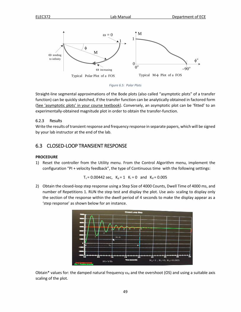
ELEC372 Lab Manual Department of ECE
49
M
ω = 0
ω increasing
ω tending to infinity
φ
1 1M
φο
0ο0−90ο
Typical Polar Plot of a FOS Typical M-φ Plot of a FOS
Figure 6.5: Polar Plots
Straight-line segmental approximations of the Bode plots (also called “asymptotic plots” of a transfer function) can be quickly sketched, if the transfer function can be analytically obtained in factored form (See ‘asymptotic plots’ in your course textbook). Conversely, an asymptotic plot can be ‘fitted’ to an experimentally-obtained magnitude plot in order to obtain the transfer-function.
6.2.3 Results Write the results of transient response and frequency response in separate papers, which will be signed by your lab instructor at the end of the lab.
6.3 CLOSED-LOOP TRANSIENT RESPONSE
PROCEDURE 1) Reset the controller from the Utility menu. From the Control Algorithm menu, implement the
configuration “PI + velocity feedback”, the type of Continuous time with the following settings:
Ts = 0.00442 sec, Kp = 1 Ki = 0 and Kd = 0.005
2) Obtain the closed-loop step response using a Step Size of 4000 Counts, Dwell Time of 4000 ms, and number of Repetitions 1. RUN the step test and display the plot. Use axis- scaling to display only the section of the response within the dwell period of 4 seconds to make the display appear as a ‘step response’ as shown below for an instance.
tN
1
2
3 4 5 6
N=8
7 8
Kp=1 , Ki=0, Kd=0.005 PI+Vfb
Obtain* values for: the damped natural frequency ωd and the overshoot (OS) and using a suitable axis scaling of the plot.

ELEC372 Lab Manual Department of ECE
50
Finding ωd : The frequency ωd can be found by finding the peak time tp. Then, the corresponding radian frequency is given by 𝜔𝜔𝑑𝑑 = 𝜋𝜋
𝑇𝑇𝑝𝑝.
Finding OS: The OS can be found by re-scaling the left axis to display values from 4000 Counts. The magnitude difference between the first positive peak1 X1 and 4000 is the OS. The percent overshoot (PO) is then given by
PO =100
−
40004000X1 % (6.4)
First maximum value
3) Export raw data into a data file for further MATLAB analysis.
4) Repeat Steps 1 and 2 for Kp values of 0.7, 0.4, 0.1 and obtain the corresponding values of ωd and the OS. Note that in each case the controller may be reset from the ‘Set Algorithm’ menu by clicking on ‘Implement’ after each change in the Kp value is made.
RESULTS
1) Tabulate ωd and OS values for the above cases. 2) Write a brief summary about the difference between open-loop and closed-loop system? 3) From the OS values, use Equation (6.2) to calculate and tabulate the values of ζ, corresponding to
the four Kp values used. Obtain a plot showing the effect of increasing Kp on the damping ratio ζ and comment on the result.
4) From the tabulated values of ζ and ωd, determine the corresponding ωn values. Obtain a plot showing the effect of increasing Kp on the natural frequency ωn and comment on the result.
ANALYSIS in MATLAB*
1) Use the following settings: Ts = 0.00442 sec, Kp = 0.1 Ki = 0 and Kd = 0.005 and the obtained model in Experiment #2, write MATLAB code to calculate CLTF in the configuration of “PI + velocity feedback” , see formula 6.3.
1 After the plot is displayed, selecting ‘Axis Scaling’ will show the ‘left axis’ scales as ‘From..., To...’. The value indicated in the ‘To...’ box is an accurate figure for the first maximum value X1 from which the PO can be readily deduced. This is shown in the next figure.
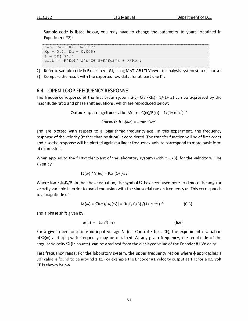
ELEC372 Lab Manual Department of ECE
51
Sample code is listed below, you may have to change the parameter to yours (obtained in Experiment #2):
2) Refer to sample code in Experiment #1, using MATLAB LTI Viewer to analysis system step response. 3) Compare the result with the exported raw data, for at least one Kp.
6.4 OPEN-LOOP FREQUENCY RESPONSE The frequency response of the first order system G(s)=C(s)/R(s)= 1/(1+τs) can be expressed by the magnitude-ratio and phase shift equations, which are reproduced below:
Output/input magnitude ratio: M(ω) = C(ω)/R(ω) = 1/(1+ ω2τ2)0.5
Phase-shift: φ(ω) = − tan-1(ωτ)
and are plotted with respect to a logarithmic frequency-axis. In this experiment, the frequency response of the velocity (rather than position) is considered. The transfer function will be of first-order and also the response will be plotted against a linear frequency-axis, to correspond to more basic form of expression.
When applied to the first-order plant of the laboratory system (with τ =J/B), for the velocity will be given by
Ω(ω) / Vi (ω) = Ko/ (1+ jωτ)
Where Ko= KeKaKt/B. In the above equation, the symbol Ω has been used here to denote the angular velocity variable in order to avoid confusion with the sinusoidal radian frequency ω. This corresponds to a magnitude of
M(ω) = |Ω(ω)/ Vi (ω)| = (KeKaKt/B) /(1+ ω2τ2)0.5 (6.5)
and a phase shift given by:
φ(ω) = - tan-1(ωτ) (6.6)
For a given open-loop sinusoid input voltage Vi (i.e. Control Effort, CE), the experimental variation of Ω(ω) and φ(ω) with frequency may be obtained. At any given frequency, the amplitude of the angular velocity Ω (in counts) can be obtained from the displayed value of the Encoder #1 Velocity.
Test frequency range: For the laboratory system, the upper frequency region where φ approaches a 90o value is found to be around 1Hz. For example the Encoder #1 velocity output at 1Hz for a 0.5 volt CE is shown below.
K=5, B=0.002, J=0.02; Kp = 0.1, Kd = 0.005; s = tf('s'); cltf = (K*Kp)/(J*s^2+(B+K*Kd)*s + K*Kp);

ELEC372 Lab Manual Department of ECE
52
Response at 1 Hz for CE=0.5 volt
The CE (input) variations can be observed in the CE window in this area of the screen
tphi
Ignoring the initial (transient) part of the display, the phase shift φ is found from the time difference tphi between two adjacent peaks:
φ = − 360 f tphi (degrees)
where f is the frequency in Hz and the negative sign is included to indicate that the output lags the input. In the above figure, for example, tphi≈0.25 sec yield to φ≈−90o which is the high-frequency limit for the first-order transfer function under consideration.
Another point regarding the test that must be mentioned is the initial (or transient) part. The system shows a certain delay before turntable action is observed, and this delay is greater for lower values of the test frequency. However, system activity is indicated by the changing numbers in the ‘Control Effort’ window at the top left of the screen, which shows the sinusoidal variation of Vi.
PROCEDURE:
1) Under ‘Data Acquisition’ menu, make sure that Control Effort (CE) has been added to the list. Reset the controller from the UTILITY menu. Set up the ‘plot’ to display the Encoder #1 Velocity on the left axis and the CE on the right axis.
2) From the COMMAND menu, select ‘Trajectory’ and choose Sinusoidal and then click on ‘Set Up’. Then select OPEN LOOP, Amplitude 0.4 volts, Frequency 0.06 Hz, and number of Repetitions 8. Next, go to ‘Execute’ and RUN the test. (Remember the point mentioned above about a delay in action.) After the data has been acquired, plot the output. (The trace will be similar to the one shown earlier for 1 Hz.)
3) Ignoring the initial transient part*, measure the constant peak-to-peak angular velocity output magnitude Ωpp in counts/sec. Also measure the time difference tphi between two adjacent peaks in order to estimate the phase shift. Use the right end of the display. Axis Scaling may be used to examine a section of the steady state display.

ELEC372 Lab Manual Department of ECE
53
4) Using Steps 2-3 above as a guide, obtain values for Ωpp (in counts/sec.) and φ (in degrees) for frequencies of 0.04, 0.08, 0.1 and 0.2 Hz.
Two typical displays are shown below.
Obtain records for each of the above mentioned frequencies, and ‘full screen’ displays and obtain the required data as accurately as possible by visual observation.
Tabulate the values of radian frequency ω(radians/sec), Ωpp (counts/sec.) and φo.
5) Sweep frequency display: From the COMMAND menu, select ‘Trajectory’, Sine Sweep. Then click on ‘Set Up’. Then select OPEN LOOP, Amplitude 0.5 volts, Frequency range from 0.02 Hz to 0.09 Hz, Sweep Time (Linear Sweep) 50 sec. Under ‘Set Up Plot’ select ‘linear frequency’ sweep. Go to ‘Execute’ and RUN the test. After the data has been acquired, plot the output and minimize the plot. Then re-plot the data using ‘logarithmic frequency’ sweep. Typical linear and log frequency plots are shown in the screen photograph below.
In these plots, the upper envelope of the plot (as shown by the dotted lines) gives the approximate ‘shape’ of the magnitude frequency response as explained in Expt#1.
RESULTS:
1) Using the data tabulated in Step 4 above, use the conversion factor Ke to convert the values of Ωpp
(counts/sec.) to Ωpp (radians/sec.). Plot Ωpp (radians/sec.) against the radian frequency ω using a linear scale.
2) Assuming that the input remained constant, the output magnitude should also be a constant (say, Y) at low frequencies approaching 0 Hz. Using the magnitude equation it can be shown that the output magnitude will drop to (1/ 2 )Y or 0.707Y when ωc = 1/τ, where ωc is called the ‘cut-off

ELEC372 Lab Manual Department of ECE
54
frequency’ or ‘break frequency’. Assuming Y is the magnitude corresponding to the frequency of 0.04 Hz, determine ωc and hence find τ. How does this value compare with the value found in EXPR#2(Sect4.3.2)? Comment on any difference observed. (The value of τ = 1/ωc can also be estimated by finding fc =1/2πωc where the phase shift is − 45o.)
6.5 CLOSED-LOOP FREQUENCY RESPONSE In this experiment, frequency-response measurements are made on the ‘optimum’ closed-loop control system that was set up at the end of the experiment 5.3.2. The magnitude response is also obtained by a ‘swept-frequency’ measurement procedure (available in the ECP Model 220 equipment) in which the frequency is increased either logarithmically or linearly over a given range while automatically acquiring and plotting output magnitude data.
6.5.1 SPOT-FREQUENCY MEASUREMENT 1) From the Utility menu, reset the controller. Implement the PID configuration of #1, with the
controller values that you selected for ‘best performance’ from last experiment 5.3.2, PID-Control. Using a step size of 4000 Counts, dwell time of 4000ms, number of repetitions 1. Verify that the ‘desirable’ response that you had selected is obtained.
2) Next, from the ‘Command’ > ‘Trajectory’ > ‘Sinusoidal’ menu, set up a sinewave input of 500 Counts amplitude, Frequency 0.5 Hz, number of repetitions 10. From ‘setup plot’ choose both ‘commanded position’ and ‘Encoder #1 Position’ on the Left axis. Then, RUN the test. The very slow sinusoidal motion of the mechanism will be observed. A typical display is shown below.
Repeat the test at another five well-spaced ‘spot’ frequencies in the range of 1 to 8 Hz. In each case, use ‘Axis Scaling’ to ‘expand’ and display the region beyond the initial (transient) part where the input shows a constant value of ± 500 Counts (1000 Cts, peak-to-peak). Use the scaled display to determine the magnitude ratio M and the phase shift φ: M is found by calculating the ratio between output and input peak-to-peak amplitudes. Phase shift φ is found by finding the time-difference tphi between adjacent peaks of the output and input waveforms and then using the equation φ= - 360 f tphi (degrees), (Note: Since the output lags inputs, a negative sign is added) where f is the frequency in Hz. Typical plots at 3 Hz, for both original and axis-scaled versions are shown below.

ELEC372 Lab Manual Department of ECE
55
3) Make a three-column table of values of frequency f (Hz), Peak-Peak Output (Counts) and tphi (sec) and enter the six sets of data in the table.
RESULTS:
1) Use the data table obtained in Step 3 to calculate and tabulate M(dB) and φ(degrees) against ω=2πf (radians/sec). Obtain Bode magnitude and phase plots for the frequency range 0.05 to 8 Hz (~0.3 to 50.3 radians/sec). Use 3-cycle semi-logarithmic graph paper. Also draw the corresponding polar plot for your data range.
2) Attempt to fit the Bode magnitude data to an asymptotic plot and hence obtain an approximate transfer function.
6.5.2 SWEEP FREQUENCY MEASUREMENT The Command/trajectory menu also offers the facility of displaying the nature of the magnitude-frequency response curve, by choosing the “sine sweep” trajectory. The input signal amplitude, the frequency sweep range, the sweep-time as well as the frequency-sweep mode (either linear or logarithmic) can be specified under Set Up. The vertical axis may be selected to show either linear or dB values. The positive side of the output envelope in the display will indicate the shape of the magnitude-frequency response and the frequency at which a peak occurs can be identified. It must be noted, however, that the displayed shape is only an approximation (especially dependent on the sweep-time) since the excitation time at each frequency may not be sufficient for the system to have reached steady state conditions.
PROCEDURE:
1) From the Utility menu, reset the controller. Implement the PID configuration of #1, with the controller values that you selected for ‘best performance’ from last experiment 5.3.2, PID-Control. Using a step size of 4000 Counts, dwell time of 4000ms, number of repetitions 1.
2) Use Set Up Trajectory and choose “Sinusoidal sweep”. Setup an input of 500 Counts amplitude, Start frequency 0.05 Hz, End frequency 8Hz, linear sweep and a sweep time of 50 sec. From ‘setup plot’ choose both ‘commanded position’ and ‘Encoder #1 Position’ on the Left axis. Then RUN the test. After a short delay, the sinusoidal motion of the rotary mechanism starting at the low frequency and increasing will be observed. Allow sufficient time for data acquisition to be completed and then display the plot. Typical sweep linear-frequency and log-frequency displays are shown below:
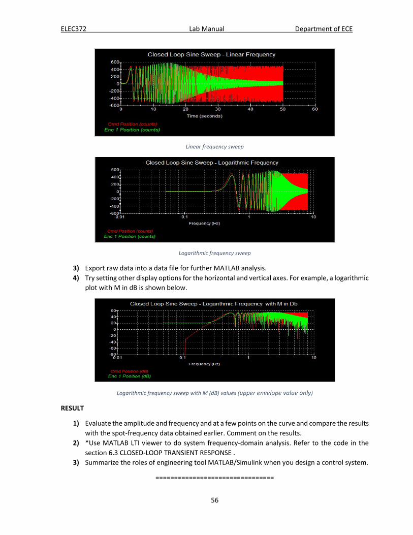
ELEC372 Lab Manual Department of ECE
56
Linear frequency sweep
Logarithmic frequency sweep
3) Export raw data into a data file for further MATLAB analysis. 4) Try setting other display options for the horizontal and vertical axes. For example, a logarithmic
plot with M in dB is shown below.
Logarithmic frequency sweep with M (dB) values (upper envelope value only)
RESULT
1) Evaluate the amplitude and frequency and at a few points on the curve and compare the results with the spot-frequency data obtained earlier. Comment on the results.
2) *Use MATLAB LTI viewer to do system frequency-domain analysis. Refer to the code in the section 6.3 CLOSED-LOOP TRANSIENT RESPONSE .
3) Summarize the roles of engineering tool MATLAB/Simulink when you design a control system.
================================

ELEC372 Lab Manual Department of ECE
57
7 EXPT #5: LAG AND LEAD COMPENSATION
7.1 OBJECTIVE - To study the concepts of lag and lead compensation and their use in improving system response. - To study the response of a system under feedback with the PID + Notch configuration. - To design a compensator by MATLAB Sisotool and verify the design on Model220.
7.2 INTRODUCTION From the past experiments it has been seen that the transient as well as steady state performance of a closed loop feedback control system is completely dependent on the OLTF. The performance of the system can therefore be modified to conform to certain given specifications by changing the OLTF. These operations basically alter the pole-zero configuration of the OLTF in such a way that the root-locus passes through the s-plane locations which are compatible with the desired specifications. In many cases, such an OLTF change can be achieved by inserting simple passive compensating feedback loop. These networks have the general transfer-function Gcomp(s) = (s + z)/(s+ p), the values of z and p being determined by the circuit elements of the inserted network. When the network is inserted in the forward path, it is called a “cascade compensation network”, whereas it is called a “feedback compensation network” if it is inserted in the feedback path. The insertion in either case is made at a point where the signal level is relatively low, such as just after the input comparator or at the output of the feedback signal transducer. From the form of Gcomp(s) it is clear that these networks introduce a real-axis pole-zero pair in the pole-zero diagram of the OLTF, usually consist of a first-order passive RC network. Two particularly simple networks used are the lag network and the lead network, their names being derived from the additional (sinusoidal) phase-shift φ introduced, which is given by
φ = tan-1(ω/z) - tan-1(ω/p)
For a lag network, φ is negative, requiring the pole to be located closer to the origin than the zero. Similarly for a lead network, the phase angle is positive and the zero must be located closer to the origin than the pole.
Lag compensation is used when the transient behavior of the uncompensated system is satisfactory but the steady state error must be improved. This is achieved by placing both z and p such that the net angle contributed at the location of the dominant poles is small while maintaining a significant (z/p) magnitude ratio. If this net angle is small, then there will be little effect on the transient response. However, the z/p ratio (>1) can still be large enough to increase the error coefficient by an amount that is sufficient to obtain the desired steady state error specification (see section 5.2). In general, the pole will have to be located very close to the origin, in order to yield an appreciable z/p ratio. Viewed in the sinusoidal frequency domain, the lag network is equivalent to a low pass filter (LPF), the low-frequency gain of the filter being used to improve the steady state error. The cutoff frequency of the LPF is chosen so that the phase-shift of the filter will not affect the phase-margin (of the uncompensated system) which is related to the transient response.
Lead compensation is used to improve the transient behavior of an uncompensated system. This is achieved by selecting z and p so that the net angle introduced will ‘bend’ the root locus and make it pass through the desired locations in the s-plane. Viewed in the frequency domain, the lead network is
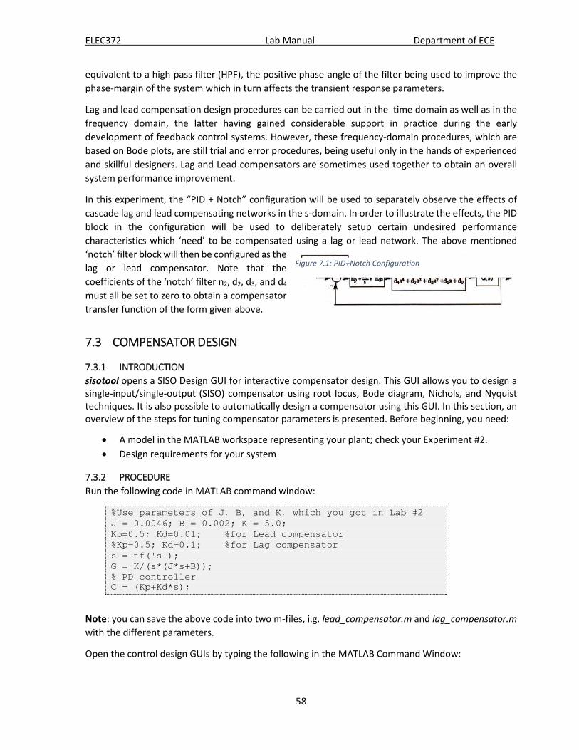
ELEC372 Lab Manual Department of ECE
58
equivalent to a high-pass filter (HPF), the positive phase-angle of the filter being used to improve the phase-margin of the system which in turn affects the transient response parameters.
Lag and lead compensation design procedures can be carried out in the time domain as well as in the frequency domain, the latter having gained considerable support in practice during the early development of feedback control systems. However, these frequency-domain procedures, which are based on Bode plots, are still trial and error procedures, being useful only in the hands of experienced and skillful designers. Lag and Lead compensators are sometimes used together to obtain an overall system performance improvement.
In this experiment, the “PID + Notch” configuration will be used to separately observe the effects of cascade lag and lead compensating networks in the s-domain. In order to illustrate the effects, the PID block in the configuration will be used to deliberately setup certain undesired performance characteristics which ‘need’ to be compensated using a lag or lead network. The above mentioned ‘notch’ filter block will then be configured as the lag or lead compensator. Note that the coefficients of the ‘notch’ filter n2, d2, d3, and d4
must all be set to zero to obtain a compensator transfer function of the form given above.
7.3 COMPENSATOR DESIGN
7.3.1 INTRODUCTION sisotool opens a SISO Design GUI for interactive compensator design. This GUI allows you to design a single-input/single-output (SISO) compensator using root locus, Bode diagram, Nichols, and Nyquist techniques. It is also possible to automatically design a compensator using this GUI. In this section, an overview of the steps for tuning compensator parameters is presented. Before beginning, you need:
• A model in the MATLAB workspace representing your plant; check your Experiment #2. • Design requirements for your system
7.3.2 PROCEDURE Run the following code in MATLAB command window:
Note: you can save the above code into two m-files, i.g. lead_compensator.m and lag_compensator.m with the different parameters.
Open the control design GUIs by typing the following in the MATLAB Command Window:
%Use parameters of J, B, and K, which you got in Lab #2 J = 0.0046; B = 0.002; K = 5.0; Kp=0.5; Kd=0.01; %for Lead compensator %Kp=0.5; Kd=0.1; %for Lag compensator s = tf('s'); G = K/(s*(J*s+B)); % PD controller C = (Kp+Kd*s);
Figure 7.1: PID+Notch Configuration

ELEC372 Lab Manual Department of ECE
59
This command opens the Control and Estimation Tools Manager - SISO design tool.
1. Define the control architecture for your system. a. In the Architecture tab of the Control and Estimation Tools Manager, click Control
Architecture. b. In the Control Architecture dialog box, select the desired control architecture which is
the first option for this experiment. c. Specify the sign of summing junctions as + or -.
2. Specify the plant model and initial values for the compensator elements in the control architecture.
a. In Architecture tab of the Control and Estimation Tools Manager, click System Data. b. In the System Data dialog box, browse for a model in the MATLAB® workspace. For G
and C, select the model G and C in workspace, which is generated from above your MATLAB commands.
3. Evaluate the system's closed-loop performance. a. Plot the system response. In the Analysis Plots tab, select a plot type - Step. Here we
are interested in closed loop r to y which is the closed loop response of the output with respect to input.
b. Display specific performance characteristic for your system. i. Right-click to select performance characteristics. For step response by right
clicking on the plot, from characteristic option you can choose peak response, settling time, rise time, and steady state.
ii. After choosing a performance characteristic, click on the dot that appears to view the characteristic value.
c. Fill the values into the table 2 or 3, which will be compared with the results on Model220 later.
sisotool

ELEC372 Lab Manual Department of ECE
60
4. Add a first-order compensator. In the tab of Compensator Editor, right click the Pole/Zero tab to add:
a. A real pole and a real zero,
• for Lead compensator, p= -17, z =-8 • for Lag compensator, p = – 0.05 z= – 2 .
b. Click the button ‘Store Design’ c. Do the above Step 3 again and record the system performance. d. Change the z/p ratio, which results in a different performance in transient response.
For example, (note: you can assign some different values).
• Lead compensator, p = – 34, z = – 4. • Lag compensator, p = – 0.1, z = – 1.
5. Refine compensator design a. Right-click on the plot ‘Step response’ and select ‘design requirements’, then choose
‘new’, set the design requirement type as:
• Lead: Rise Time <0.02s, Settling time <0.2s, Percent overshoot <20.0%.
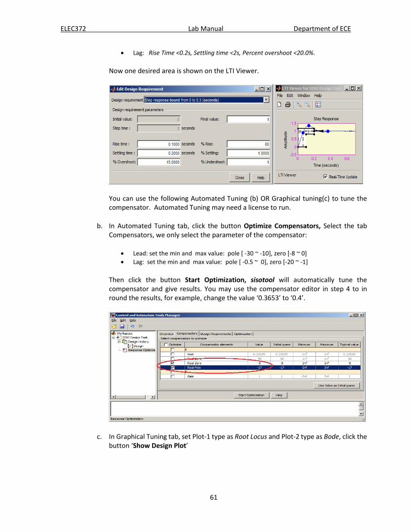
ELEC372 Lab Manual Department of ECE
61
• Lag: Rise Time <0.2s, Settling time <2s, Percent overshoot <20.0%.
Now one desired area is shown on the LTI Viewer.
You can use the following Automated Tuning (b) OR Graphical tuning(c) to tune the compensator. Automated Tuning may need a license to run.
b. In Automated Tuning tab, click the button Optimize Compensators, Select the tab Compensators, we only select the parameter of the compensator:
• Lead: set the min and max value: pole [ -30 ~ -10], zero [-8 ~ 0] • Lag: set the min and max value: pole [ -0.5 ~ 0], zero [-20 ~ -1]
Then click the button Start Optimization, sisotool will automatically tune the compensator and give results. You may use the compensator editor in step 4 to in round the results, for example, change the value ‘0.3653’ to ‘0.4’.
c. In Graphical Tuning tab, set Plot-1 type as Root Locus and Plot-2 type as Bode, click the button ‘Show Design Plot’
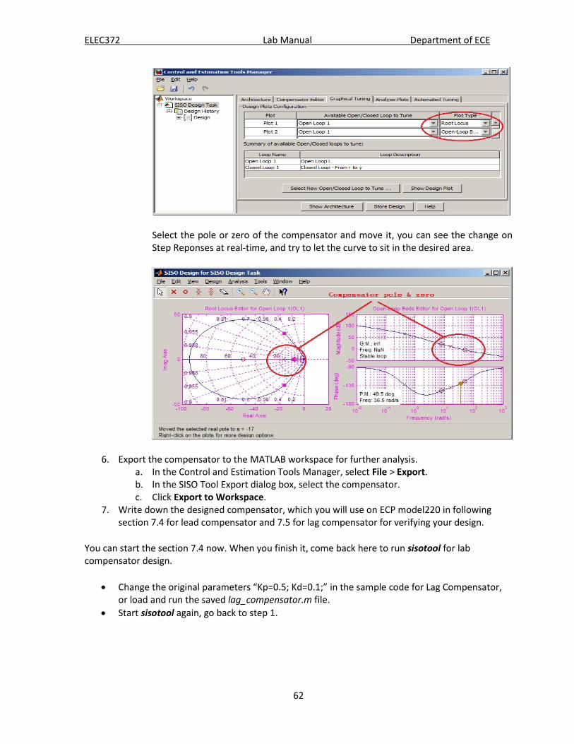
ELEC372 Lab Manual Department of ECE
62
Select the pole or zero of the compensator and move it, you can see the change on Step Reponses at real-time, and try to let the curve to sit in the desired area.
6. Export the compensator to the MATLAB workspace for further analysis. a. In the Control and Estimation Tools Manager, select File > Export. b. In the SISO Tool Export dialog box, select the compensator. c. Click Export to Workspace.
7. Write down the designed compensator, which you will use on ECP model220 in following section 7.4 for lead compensator and 7.5 for lag compensator for verifying your design.
You can start the section 7.4 now. When you finish it, come back here to run sisotool for lab compensator design.
• Change the original parameters “Kp=0.5; Kd=0.1;” in the sample code for Lag Compensator, or load and run the saved lag_compensator.m file.
• Start sisotool again, go back to step 1.

ELEC372 Lab Manual Department of ECE
63
7.4 LEAD COMPENSATION
7.4.1 PROCEDURE 1) Reset the controller from the Utility menu. From the Set Up Control Algorithm menu, the type of
Continuous time, implement Figure 7.1: PID+Notch Configuration with Kp = 0.5, Ki =0 and Kd = 0.01. In the notch filter block, set n0 = 1, n1 = n2 = 0 for the numerator coefficients and d0 = 1 and d1 = d2 = d3 = d4 = 0 for the denominator coefficients. This makes the filter a unity-gain block. Set up a closed-loop step response using a step size of 10000 Counts, dwell time of 4000ms, number of repetitions 1. RUN the step test. A slightly underdamped response should result with zero step error as shown by the typical response below. Measure* the overshoot OS. Now let us assume that we need to reduce the OS (i.e. improve the transient response) using a lead compensator. Fill the result into the row 1 in Table 2.
2) Re-implement the controller with the same coefficients in the PID block, but with the filter block coefficients changed to n0 = d0 = 1, n1 = 1/z = 1/8, d1 = 1/p = 1/17 and all the other coefficients zero. This yields the lead transfer function(𝑠𝑠
8+ 1)/( 𝑠𝑠
17+ 1) .
Obtain the step response using the same step input as before. An improvement in the OS should result as seen in the typical plot shown below. Measure* the overshoot OS, Fill the result into the row 2 in Table 2.
3) Change the zero and pole according to the row 3 in Table 2, repeat step 2 and write down the result. 4) Implement the controller exported from Sisotool for Lead Compensator design in section 7.3. Fill
the result into the row 4 in Table 2.
Table 2: Lead Compensator, Kp=0.5, Kd=0.01
No Lead Rise Time Settling time Percent overshoot Zero Pole MATLAB ECP220 MATLAB ECP220 MATLAB ECP220
1 - - 2 8 17 3 4 <0.02s <0.2s <20%
7.4.2 RESULTS 1) Compare the two overshoots obtained in Steps 1-3 above and attempt to correlate the result with
the lead network pole-zero values by using the root locus with and without the compensator. 2) Comment on the results of the other two z/p ratios used. 3) Compare the design on Sisotool and actual performance on Model 220.
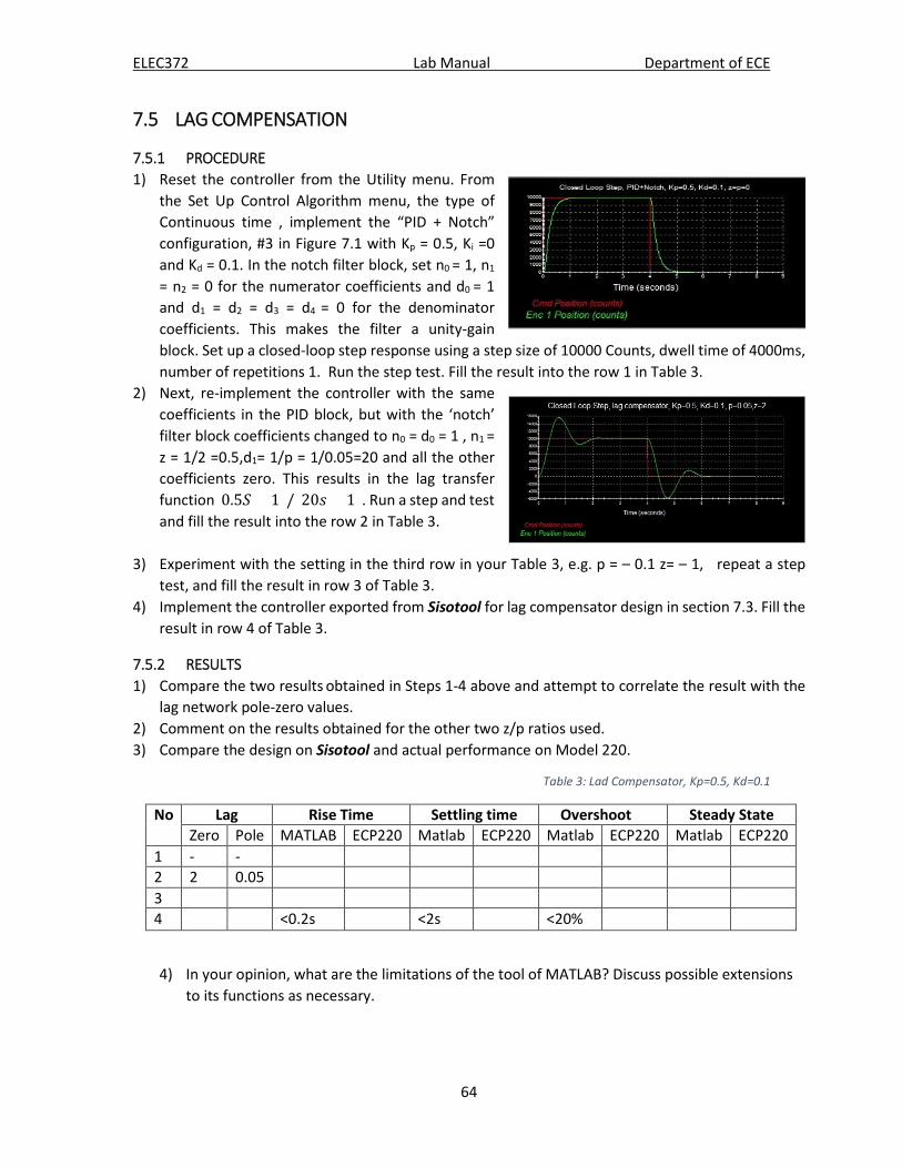
ELEC372 Lab Manual Department of ECE
64
7.5 LAG COMPENSATION
7.5.1 PROCEDURE 1) Reset the controller from the Utility menu. From
the Set Up Control Algorithm menu, the type of Continuous time , implement the “PID + Notch” configuration, #3 in Figure 7.1 with Kp = 0.5, Ki =0 and Kd = 0.1. In the notch filter block, set n0 = 1, n1
= n2 = 0 for the numerator coefficients and d0 = 1 and d1 = d2 = d3 = d4 = 0 for the denominator coefficients. This makes the filter a unity-gain block. Set up a closed-loop step response using a step size of 10000 Counts, dwell time of 4000ms, number of repetitions 1. Run the step test. Fill the result into the row 1 in Table 3.
2) Next, re-implement the controller with the same coefficients in the PID block, but with the ‘notch’ filter block coefficients changed to n0 = d0 = 1 , n1 = z = 1/2 =0.5,d1= 1/p = 1/0.05=20 and all the other coefficients zero. This results in the lag transfer function(0.5𝑆𝑆 + 1)/(20𝑠𝑠 + 1). Run a step and test and fill the result into the row 2 in Table 3.
3) Experiment with the setting in the third row in your Table 3, e.g. p = – 0.1 z= – 1, repeat a step test, and fill the result in row 3 of Table 3.
4) Implement the controller exported from Sisotool for lag compensator design in section 7.3. Fill the result in row 4 of Table 3.
7.5.2 RESULTS 1) Compare the two results obtained in Steps 1-4 above and attempt to correlate the result with the
lag network pole-zero values. 2) Comment on the results obtained for the other two z/p ratios used. 3) Compare the design on Sisotool and actual performance on Model 220.
Table 3: Lad Compensator, Kp=0.5, Kd=0.1
No Lag Rise Time Settling time Overshoot Steady State Zero Pole MATLAB ECP220 Matlab ECP220 Matlab ECP220 Matlab ECP220
1 - - 2 2 0.05 3 4 <0.2s <2s <20%
4) In your opinion, what are the limitations of the tool of MATLAB? Discuss possible extensions to its functions as necessary.

ELEC372 Lab Manual Department of ECE
65
APPENDIX-A: EXPECTATIONS OF ORIGINALITY
Faculty of Engineering and Computer Science
Expectations of Originality
This form sets out the requirements for originality for work submitted by students in the Faculty of Engineering and Computer Science. Submissions such as assignments, lab reports, project reports, computer programs and take-home exams must conform to the requirements stated on this form and to the Academic Code of Conduct. The course outline may stipulate additional requirements for the course.
1. Your submissions must be your own original work. Group submissions must be the original work of the students in the group.
2. Direct quotations must not exceed 5% of the content of a report, must be enclosed in quotation marks, and must be attributed to the source by a numerical reference citation2. Note that engineering reports rarely contain direct quotations.
3. Material paraphrased or taken from a source must be attributed to the source by a numerical reference citation.
4. Text that is inserted from a web site must be enclosed in quotation marks and attributed to the web site by numerical reference citation.
5. Drawings, diagrams, photos, maps or other visual material taken from a source must be attributed to that source by a numerical reference citation.
6. No part of any assignment, lab report or project report submitted for this course can be submitted for any other course.
7. In preparing your submissions, the work of other past or present students cannot be consulted, used, copied, paraphrased or relied upon in any manner whatsoever.
8. Your submissions must consist entirely of your own or your group’s ideas, observations, calculations, information and conclusions, except for statements attributed to sources by numerical citation.
9. Your submissions cannot be edited or revised by any other student. 10. For lab reports, the data must be obtained from your own or your lab group’s experimental
work. 11. For software, the code must be composed by you or by the group submitting the work,
except for code that is attributed to its sources by numerical reference.
You must write one of the following statements on each piece of work that you submit:
2 Rules for reference citation can be found in “Form and Style” by Patrich MacDonagh and Jack Bordan, fourth edition, May, 2000, available at http://www.encs.concordia.ca/scs/Forms/Form&Style.pdf. Approved by the ENCS Faculty Council February 10, 2012

ELEC372 Lab Manual Department of ECE
66
For individual work: “I certify that this submission is my original work and meets the Faculty's Expectations of Originality”, with your signature, I.D. #, and the date.
For group work: “We certify that this submission is the original work of members of the group and meets the Faculty's Expectations of Originality”, with the signatures and I.D. #s of all the team members and the date.
A signed copy of this form must be submitted to the instructor at the beginning of the semester in each course.
I certify that I have read the requirements set out on this form, and that I am aware of these requirements. I certify that all the work I will submit for this course will comply with these requirements and with additional requirements stated in the course outline.
Course Number: _________________________ Instructor: _____________________
Name: _________________________ I.D. # _____________________
Signature: _________________________ Date: _____________________