Elasticity

Managerial Economics

Jack Wu

American Airlines

“Extensive research and many years of experience have taught us that business travel demand is quite inelastic… On the other hand, pleasure travel has substantial elasticity.”

Robert L. Crandall, CEO, 1989

Own-Price Elasticity: E=Q%/P%

Definition: percentage change in quantity demanded resulting from 1% increase in price of the item.

Alternatively,

n_price%_change_i

_demandedn_quantity%_change_i

Calculating Elasticity

1.1

1.0

1.44 1.5

Calculating Elasticity

Arc Approach:

Elasticity={[Q2-Q1]/avgQ}/{[P2-P1]/avgP

% change in qty = (1.44-1.5)/1.47 = -4.1% % change in price = (1.10-1)/1.05 = 9.5% Elasticity=-4.1%/9.5%

=-0.432

Calculating Elasticity

Point approach:

Elasticity={[Q2-Q1]/Q1}/{[P2-P1]/P1}

% change in qty = (1.44-1.5)/1.5= -4%

% change in price = (1.10-1)/1= 10%

Elasticity=-4%/10%=-0.4

Own-Price Elasticity

|E|=0, perfectly inelastic 0<|E|<1, inelastic |E|=1, unit elastic |E|>1, elastic |E|=infinity, perfectly elastic

Slope/Elasticity

• steeper demand curve <--> demand less elastic

• slope not same as elasticity

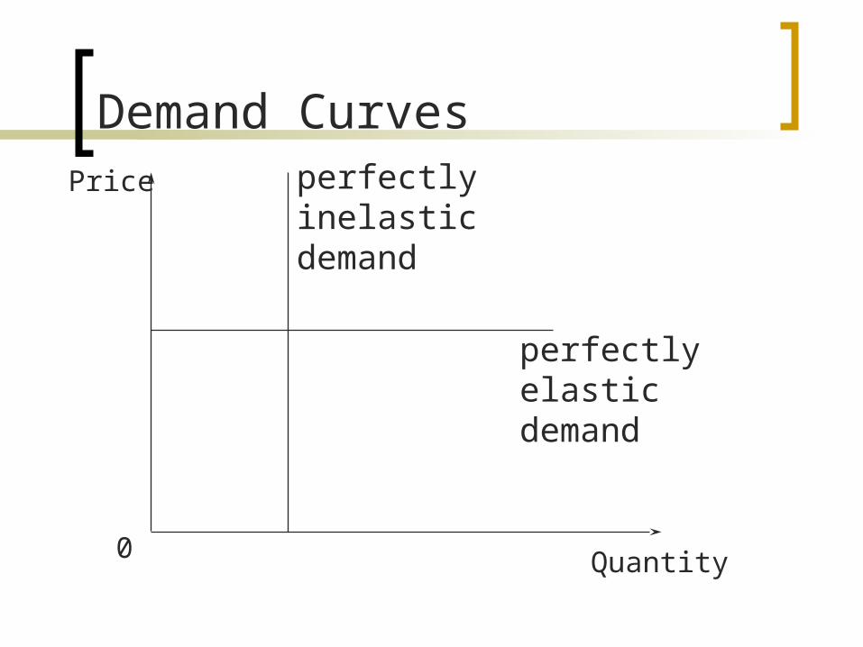
0 Quantity

Price

Demand Curves

perfectly elastic demand

perfectly inelastic demand

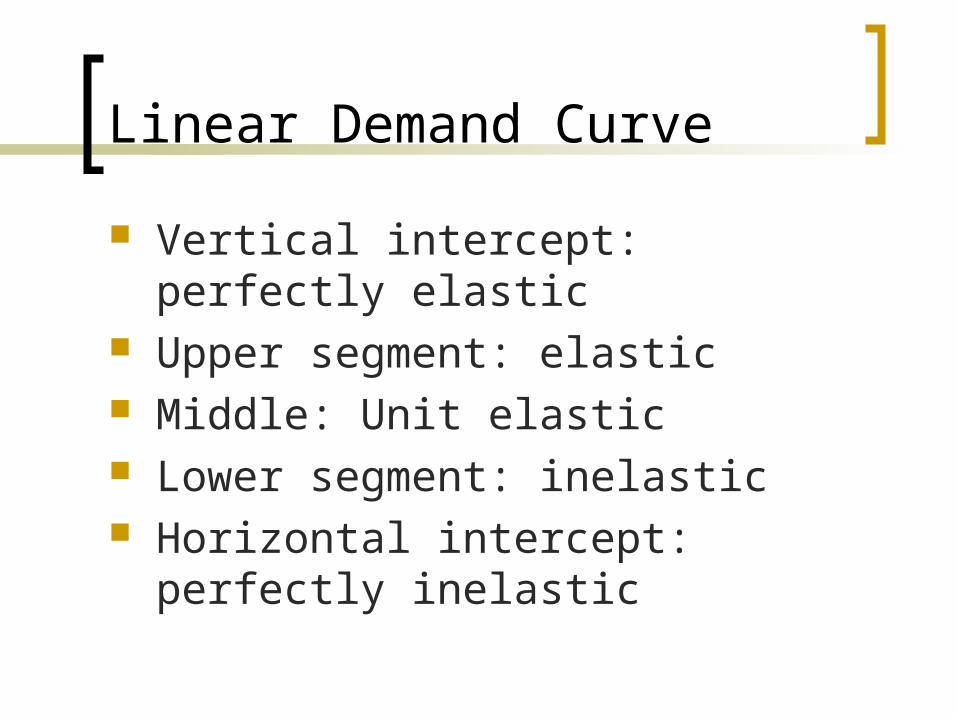
Linear Demand Curve

Vertical intercept: perfectly elastic Upper segment: elastic Middle: Unit elastic Lower segment: inelastic Horizontal intercept: perfectly inelastic

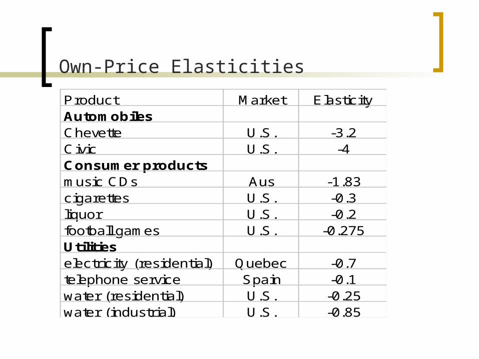
Product Market ElasticityAutomobilesChevette U.S. -3.2Civic U.S. -4Consumer productsmusic CDs Aus -1.83cigarettes U.S. -0.3liquor U.S. -0.2football games U.S. -0.275Utilitieselectricity (residential) Quebec -0.7telephone service Spain -0.1water (residential) U.S. -0.25water (industrial) U.S. -0.85

Own-Price Elasticities

Own-Price Elasticity: Determinants

availability of direct or indirect substitutes

cost / benefit of economizing (searching for better price)

buyer’s prior commitments

separation of buyer and payee

AAdvantage

1981: American Airlines pioneered frequent flyer program buyer commitment business executives fly at the expense of others

When to raise price

CEO: “Profits are low. We must raise prices.”

Sales Manager: “But my sales would fall!”

Real issue: How sensitive are buyers to price changes?

Price Increase: Expenditure

if demand elastic, expenditure will fall

if demand inelastic, expenditure will rise

Income Elasticity, I=Q%/Y%

Definition: percentage change in quantity demanded resulting from 1% increase in income.

Alternatively,

n_income%_change_i

_demandedn_quantity%_change_i

Income Elasticity

I >0, Normal good I <0, Inferior good Among normal goods:

0<I<1, necessity

I>1, luxury

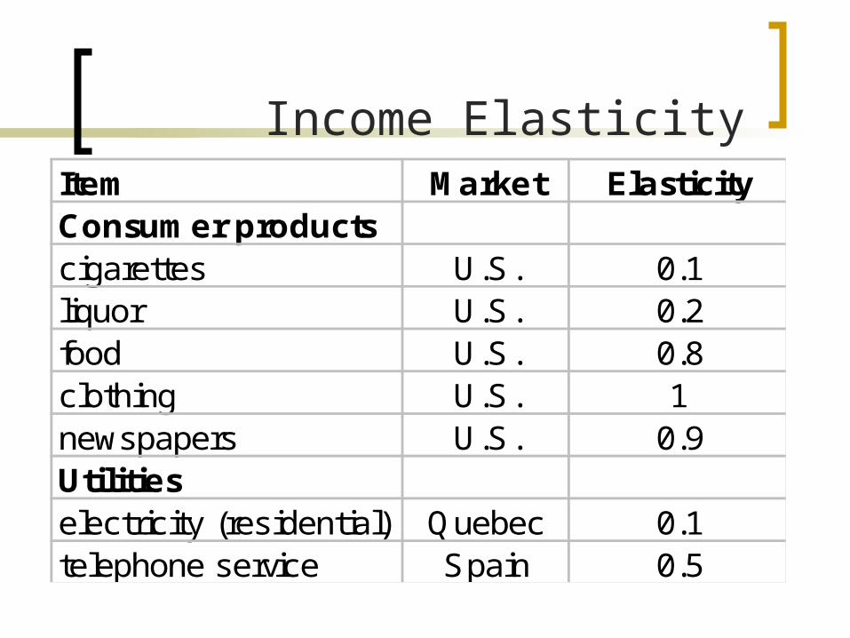
Item Market ElasticityConsumer productscigarettes U.S. 0.1liquor U.S. 0.2food U.S. 0.8clothing U.S. 1newspapers U.S. 0.9Utilitieselectricity (residential) Quebec 0.1telephone service Spain 0.5

Income Elasticity

Cross-Price Elasticity: C=Q%/Po%

Definition: percentage change in quantity demanded for one item resulting from 1% increase in the price of another item.

(%change in quantity demanded for one item) / (% change in price of another item)

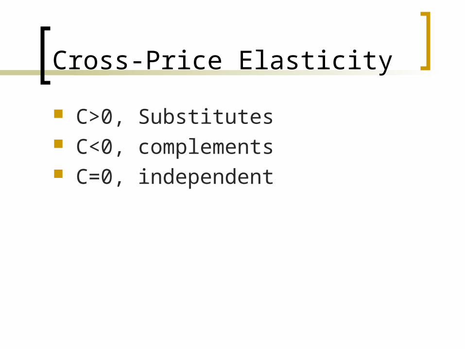
Cross-Price Elasticity

C>0, Substitutes C<0, complements C=0, independent

Item Market ElasticityConsumer productsclothing/food U.S. 0.1gasoline (competing stn) Boston, MA 1.2Utilitieselectricity/gas (residential) Quebec 0.1electricity/oil (residential) Quebec 0bus/subway London 0.25

Cross-Price Elasticities

Advertising Elasticity: a=Q%/A%

Definition: percentage change in quantity demanded resulting from 1% increase in advertising expenditure.

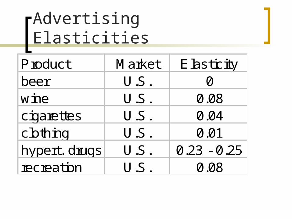
Product Market Elasticitybeer U.S. 0wine U.S. 0.08cigarettes U.S. 0.04clothing U.S. 0.01hypert. drugs U.S. 0.23 - 0.25recreation U.S. 0.08

Advertising Elasticities

Advertising

direct effect: raises demand indirect effect: makes demand less

sensitive to price

Own price elasticity for antihypertensive drugs

Without advertising: -2.05

With advertising: -1.6

Forecasting Demand

Q%=E*P%+I*Y%+C*Po%+a*A%

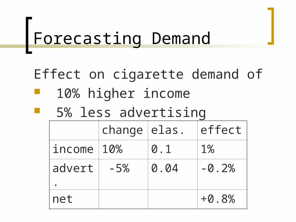
Forecasting Demand

Effect on cigarette demand of 10% higher income 5% less advertising

change elas. effect

income 10% 0.1 1%

advert. -5% 0.04 -0.2%

net +0.8%

Adjustment Time

short run: time horizon within which a buyer cannot adjust at least one item of consumption/usage

long run: time horizon long enough to adjust all items of consumption/usage

Adjustment Time

For non-durable items, the longer the time that buyers have to adjust, the bigger will be the response to a price change.

For durable items, a countervailing effect (that is, the replacement frequency effect) leads demand to be relatively more elastic in the short run.

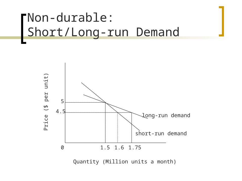
0

4.5

5

1.5 1.6 1.75

long-run demand

short-run demand

Quantity (Million units a month)

Pri

ce (

$ p

er

unit

)

Non-durable: Short/Long-run Demand

Item Factor Market Short-run Long-runNondurablescigarettes price U.S. -0.3 -3.3liquor price U.S./Canada -0.2 -1.8gaseline price U.S. -0.1 -0.5

income U.S. 0 0.3bus price London -0.8 -1.3subway price London -0.4 -0.7railway price Philadelphia -0.5 -1.8Durablesautomobiles price U.S. -0.2 -0.5

income U.S. 3 1.4

Short/Long-run Elasticities

Statistical Estimation: Data

time series – record of changes over time in one market

cross section -- record of data at one time over several markets

Panel data: cross section over time

Multiple Regression

Statistical technique to estimate the separate effect of each independent variable on the dependent variable dependent variable = variable whose changes are to be explained independent variable = factor affecting the dependent variable