eindhoven university of technology department of mathematics and … · 2009-12-03 · eindhoven...

EINDHOVEN UNIVERSITY OF TECHNOLOGY

Department of Mathematics and Computer Science

CASA-Report 09-16

May 2009

Efficient computation of three-dimensional flow

in helically corrugated hoses including swirl

by

B.J. van der Linden, E. Ory, J.A.M. Dam,

A.S. Tijsseling, M. Pisarenco

Centre for Analysis, Scientific computing and Applications

Department of Mathematics and Computer Science

Eindhoven University of Technology

P.O. Box 513

5600 MB Eindhoven, The Netherlands

ISSN: 0926-4507

Proceedings of

, , ,

CASA Report 2009-17

EFFICIENT COMPUTATION OF THREE-DIMENSIONAL FLOW IN HELICALLYCORRUGATED HOSES INCLUDING SWIRL

Bas J. van der Linden∗

CASA†

Department of MathematicsTechnische Universiteit Eindhoven

Eindhoven, The NetherlandsEmail: [email protected]

Emmanuel OrySingle Buoy Mooring Offshore

Monaco, MonacoEmail: [email protected]

Jacques DamStork Inoteq

Amsterdam, The NetherlandsEmail: [email protected]

Arris S. TijsselingCASA



Maxim PisarencoCASA



ABSTRACTIn this article we propose an efficient method to compute the

friction factor of helically corrugated hoses carrying flow at highReynolds numbers. A comparison between computations of sev-eral turbulence models is made with experimental results for cor-rugation sizes that fall outside the range of validity of the Moodydiagram. To do this efficiently we implement quasi-periodicity.Using the appropriate boundary conditions and matching bodyforce, we only need to simulate a single period of the corrugationto find the friction factor for fully developed flow.

A second technique is introduced by the construction of anappropriately twisted wedge, which allows us to furthermore re-duce the problem by a further dimension while accounting for theBeltrami symmetry that is present in the full three-dimensionalproblem. We make a detailed analysis of the accuracy and time-saving that this novelty introduces.

We show that the swirl inside the flow, which is introducedby the helical boundary, has a positive effect on the friction fac-

∗Please send all communication to this author.†Centre for Analysis, Scientific Computing and Applications.

tor. Furthermore, we give a prediction for which corrugationangles the assumption of axisymmetry is no longer valid. It thenhas to make place for Beltrami-symmetry if accurate results arerequired.

1 INTRODUCTIONThis article studies the computation of friction factors of cor-

rugated hoses for turbulent flow. The friction factor or, equiva-lently, the head loss of a hose is an important design character-istic, that is used in engineering applications to make importantdesign decisions such as the required power of the pumps, thatdrive the flow, and the size of the hose’s diameter.

When flexible hoses have to resist high pressure or temper-ature loads, the hose structure needs to be reinforced. Such re-inforcement, especially when it needs to cover greater lengths,typically means winding a metal wire or other strong and thinmaterial in a spiral around a flexible hose, made of fabric. Thisreinforcement changes the internal geometry of the hose, causingcorrugations that strongly affect the flow in the hose.

1 Copyright c© by ASME

If the corrugation is small with respect to the hose’s diam-eter, it can be treated in the same way as conventional surfaceroughness as long as it is taken into account, that the rough-ness is not random but regular [1]. The Moody diagram [2] —or more conveniently the equivalent explicit formulas as listedin [3] — can be used to reliably estimate the hose’s performance.If the relative roughness exceeds 3%, however it is known thatthe Moody diagram is no longer applicable as the shape of theroughness becomes important. For the hoses of our interest, thecorrugation was 5–10% of the diameter, which means that foreach different shape of the corrugation the friction factor versusReynolds number curve needs to be computed. At a design stage,this could involve large families of hose designs and so the com-putation of the friction factor must be efficient.

The shape of the cross section of the corrugation matters inmore than one way. First of all, the size of the corrugation is solarge that the flow near the wall is visibly affected. The flow willdetach behind the corrugations, creating vortices in the troughs ofthe corrugation. At other points the flow will reattach, implyinga stagnation point with a high pressure zone around it. Then,where the protrusion of the corrugation is the greatest,s the flowwill locally contract and an underpressure will be created.

The spiral shape of the corrugations, that are discussed inthis article, have also a macroscopic effect on the flow. Becausethe pressure forces on the wall align with the normal to the wall,and the wall has a helical structure, the counterforce exerted bythe wall on the liquid has an azimuthal component. In this waythe spiral shape of the corrugation causes the flow to swirl, whichin turn affects the friction factor. Unfortunately, these observa-tions mean that we need to know the flow at a small scale andin all three dimensions, even when we are eventually only inter-ested in a global quantity, a single number: the friction factor.

In this paper we investigate how we can efficiently computethe friction factor of a helically corrugated hose without gettingstuck in lengthy computer simulations. The question, how wecan compute a global quantity both reliably and in finite time,even if it so much depends on knowing the local, small scalestructure of the flow, is answered in three steps.

After introducing the governing equations in the next sec-tion, we first reduce the problem by a whole spatial dimensionby making use of the fact that a fully developed flow is quasi-periodic. This first step is the most important as it means that wecan predict the performance of a hose of a few hundred metresby only considering a geometry of a few centimetres in length.The second computational reduction is quite straightforward forannular corrugations, but the third step shows another dimensioncan be taken out of the geometry by using the flow’s helical sym-metry. This flow involves swirl, which is studied in the sectionbefore the conclusive last section.

Figure 1. Small section of a corrugated hose.

2 NUMERICAL SIMULATION OF TURBULENT FLOWIN HOSESAs we noted in the introduction, the observation, that the

shape of the corrugation matters for the friction factor, means theflow needs to be known in full detail for an accurate predictionof the friction factor.

A small section of the type of hose that we wish to study isdisplayed in Figure 1. The diameter ranges from 10 cm to half ametre and the hoses are filled with a water-like liquid with speedsup to 5 to 10 m/s. With a density of 1000 kg/m3 and viscosityof 1 mPa · s, the Reynolds number is ReD = 106, so deep in theturbulent region. The corrugation has a height of 1–2 cm and aspiral angle of only a few degrees.

The Reynolds number is too high to study the flow in ev-ery detail, for example with Direct Numerical Simulation (DNS).Rather the turbulence needs to be modelled and estimated. For-tunately, the Reynolds number is so elevated that we can use theso-called Reynolds Averaged Navier-Stokes approximation forthe flow. For a complete understanding of the underlying pro-cesses reference [4] is recommended literature. A shorter (butless profound) road to the governing equations is given in [5],which we will follow here.

2.1 The Reynolds-Averaged Navier-Stokes equationsWhile the standard Navier-Stokes equations are equally

valid for turbulent flows, the variations in the flow happen onsuch small length and time scales, that direct numerical simula-tion becomes prohibitively expensive. The computational cost interms of number of operations of direct numerical simulation isestimated at Re3 in [4]. For a Reynolds number of about one mil-lion this means that it is too costly on today’s computer systems.


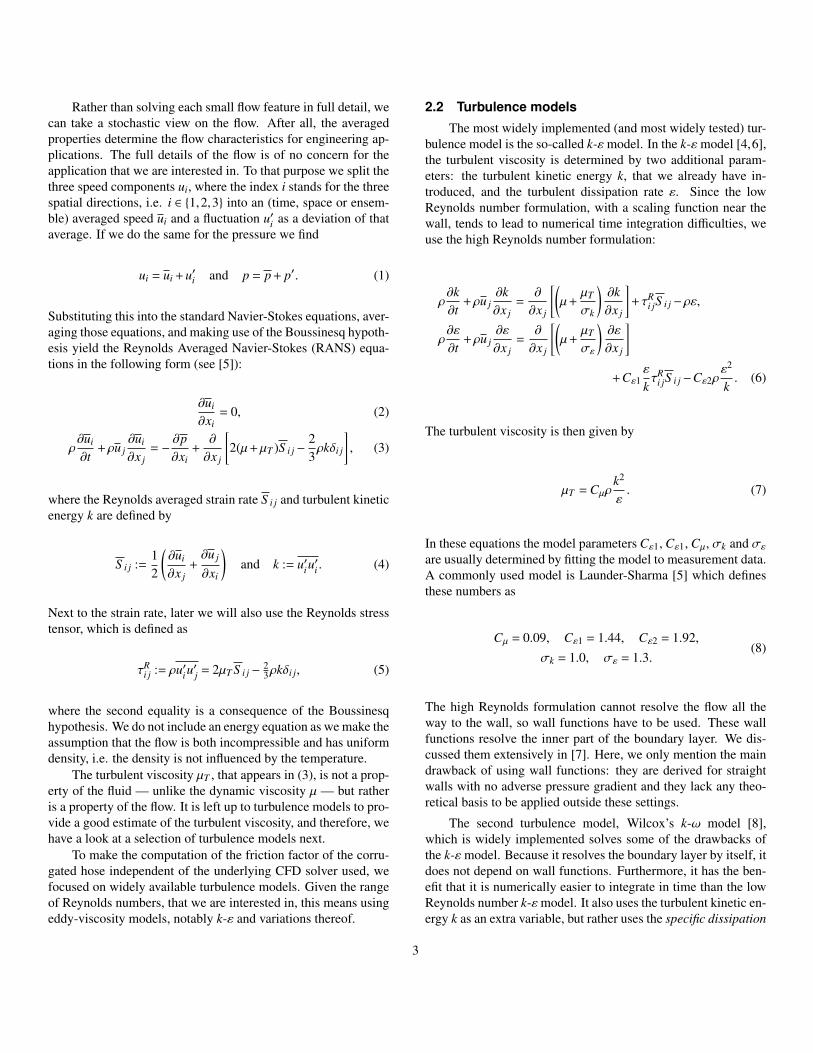
Rather than solving each small flow feature in full detail, wecan take a stochastic view on the flow. After all, the averagedproperties determine the flow characteristics for engineering ap-plications. The full details of the flow is of no concern for theapplication that we are interested in. To that purpose we split thethree speed components ui, where the index i stands for the threespatial directions, i.e. i ∈ 1,2,3 into an (time, space or ensem-ble) averaged speed ui and a fluctuation u′i as a deviation of thataverage. If we do the same for the pressure we find

ui = ui + u′i and p = p + p′. (1)

Substituting this into the standard Navier-Stokes equations, aver-aging those equations, and making use of the Boussinesq hypoth-esis yield the Reynolds Averaged Navier-Stokes (RANS) equa-tions in the following form (see [5]):

∂ui

∂xi= 0, (2)

ρ∂ui

∂t+ρu j

∂ui

∂x j= −

∂p∂xi

+∂

∂x j

[2(µ+µT )S i j−

23ρkδi j

], (3)

where the Reynolds averaged strain rate S i j and turbulent kineticenergy k are defined by

S i j :=12

(∂ui

∂x j+∂u j

∂xi

)and k := u′iu

′i . (4)

Next to the strain rate, later we will also use the Reynolds stresstensor, which is defined as

τRi j := ρu′iu

′j = 2µT S i j−

23ρkδi j, (5)

where the second equality is a consequence of the Boussinesqhypothesis. We do not include an energy equation as we make theassumption that the flow is both incompressible and has uniformdensity, i.e. the density is not influenced by the temperature.

The turbulent viscosity µT , that appears in (3), is not a prop-erty of the fluid — unlike the dynamic viscosity µ — but ratheris a property of the flow. It is left up to turbulence models to pro-vide a good estimate of the turbulent viscosity, and therefore, wehave a look at a selection of turbulence models next.

To make the computation of the friction factor of the corru-gated hose independent of the underlying CFD solver used, wefocused on widely available turbulence models. Given the rangeof Reynolds numbers, that we are interested in, this means usingeddy-viscosity models, notably k-ε and variations thereof.

2.2 Turbulence models

The most widely implemented (and most widely tested) tur-bulence model is the so-called k-ε model. In the k-ε model [4,6],the turbulent viscosity is determined by two additional param-eters: the turbulent kinetic energy k, that we already have in-troduced, and the turbulent dissipation rate ε. Since the lowReynolds number formulation, with a scaling function near thewall, tends to lead to numerical time integration difficulties, weuse the high Reynolds number formulation:

ρ∂k∂t

+ρu j∂k∂x j

=∂

∂x j

[(µ+

µT

σk

)∂k∂x j

]+τR

i jS i j−ρε,

ρ∂ε

∂t+ρu j

∂ε

∂x j=

∂

∂x j

[(µ+

µT

σε

)∂ε

∂x j

]+Cε1

ε

kτR

i jS i j−Cε2ρε2

k. (6)

The turbulent viscosity is then given by

µT = Cµρk2

ε. (7)

In these equations the model parameters Cε1, Cε1, Cµ, σk and σεare usually determined by fitting the model to measurement data.A commonly used model is Launder-Sharma [5] which definesthese numbers as

Cµ = 0.09, Cε1 = 1.44, Cε2 = 1.92,σk = 1.0, σε = 1.3.

(8)

The high Reynolds formulation cannot resolve the flow all theway to the wall, so wall functions have to be used. These wallfunctions resolve the inner part of the boundary layer. We dis-cussed them extensively in [7]. Here, we only mention the maindrawback of using wall functions: they are derived for straightwalls with no adverse pressure gradient and they lack any theo-retical basis to be applied outside these settings.

The second turbulence model, Wilcox’s k-ω model [8],which is widely implemented solves some of the drawbacks ofthe k-ε model. Because it resolves the boundary layer by itself, itdoes not depend on wall functions. Furthermore, it has the ben-efit that it is numerically easier to integrate in time than the lowReynolds number k-εmodel. It also uses the turbulent kinetic en-ergy k as an extra variable, but rather uses the specific dissipation


of turbulence ω, defined as ω := ε/k. The equations are

ρ∂k∂t

+ρu j∂k∂x j

= τRi j∂u j

∂x j−ρβ∗kω+

∂

∂x j

[(µ+σ∗ωµT )

∂k∂x j

]ρ∂ω

∂t+ρu j

∂ω

∂x j= α

ω

kτR

i j∂ui

∂x j−ρβω2 +

∂

∂x j

[(µ+σωµT )

∂ω

∂x j

].

(9)

Also, this model contains model parameters. In this case:

α = 59 , β = 3

40 , β∗ = 9100 , σω = 1

2 , σ∗ω = 12 . (10)

The turbulent dissipation rate can be found by ε = β∗ωk andthe turbulent viscosity by µT = ρk/ω. The boundary equationsare k = 0, while ω goes asymptotically to infinity for smoothwalls, which makes the boundary condition dependent on the lo-cal mesh size near the wall. For rough walls (which we havein between the corrugations, see [7]) this is not the case and wecan simply use ω = Nµ/k2

s [9] with N = 2500 and ks the surfaceroughness height.

While the k-ωmodel performs better, when adverse pressuregradients are present, it performs worse than the k-ε model inthe freestream. The third and final model that we consider isMenter’s k-ω Shear-Stress Transport (SST) model [10]. It can beseen as a combination between the two previous models, whereit uses the k-ω near the wall and k-ε away from the wall. Thisleads to much better results for adverse pressure gradients [11]and reattaching flows [12]. The equations are

ρ∂k∂t

+ρu j∂k∂x j

=∂

∂x j

[(µ+σkµT )

∂k∂x j

]+τR

i jS i j−β∗ρωk,

ρ∂ω

∂t+ρu j

∂ω

∂x j=

∂

∂x j

[(µ+σωµT )

∂ω

∂x j

]+

Cωρ

µTτR

i jS i j−β∗ρω2 + 2(1− f1)

ρσω2

ω

∂k∂x j

∂ω

∂x j, (11)

where the blending function f1 is defined by

f1 = tanh(ζ41 ),

ζ1 := minmax

√k

0.09ωd,

500µρωd2

, 4ρσω2kCDkωd2

, (12)

CDkω = max[2ρσω2

ω

∂k∂x j

∂ω

∂x j,10−20

].

Here we use d for the distance to the nearest wall. The computa-tion of the turbulent viscosity also becomes more complicated:

µT =a1ρk

max(a1ω, f2‖∇×u‖), (13)

with f2 a second blending function:

f2 = tanhζ22 , ζ2 = max

2√

k0.09ωd

,500µρωd2

. (14)

2.3 MeshingFor computational fluid dynamics constructing a mesh is of

the same importance as using the correct equations. For all vis-cous flow computations it is best that the mesh elements near thewall are aligned with the flow. But turbulence models such as k-εor k-ω SST put additional constraints on the mesh size near theboundary.

The high Re k-ε model uses wall functions and is the moreforgiving. Wall functions are semi-empirical expressions thatmodel the viscosity-affected inner region of the boundary layer(the viscous sublayer and the buffer layer). The differential equa-tions for k and ε are only responsible for the fully turbulent re-gion (where the underlying assumptions for that model are valid).Without going into the details of the wall functions (see [7] foran extensive discussion), we only mention, that the size of themesh perpendicular to the wall has to fall in a specific range:

50 ≤ y+k-ε ≤ 300. (15)

Here, y+ is the non-dimensional distance to the wall defined by

y+ = u∗y/µ, (16)

where u∗ := C1/4µ k1/2 is the shear velocity. Note, that u∗ is only

known a posteriori and so is y+, as these quantities depend on theflow itself. Meshing is therefore preferably done adaptively, orin practise with a good estimate of the resulting flow.

The k-ω and k-ω SST models can by themselves resolvenon-fully turbulent parts of the boundary layer and therefore donot need wall functions. Their independence on these empiricalrelations, which are determined for some specific flow situation,but can never be guaranteed to predict the flow correctly in othersituations, is positive. It puts a heavier burden on the mesh, how-ever, as the demand for the mesh size becomes more stringent:

y+k-ω ≈ 1. (17)


Figure 2. Example of an annularly corrugated tube.

This effectively means that the mesh size for a flow solved withone of the k-ω models is 50 to 300 times smaller than for thek-ε model. Note that k-ω SST uses the distance d to the nearestposition on the boundary, which in addition means that the meshshould be regular near the wall.

3 EFFICIENT COMPUTATION OF THE FRICTION FAC-TORThe friction factor is determined for fully developed flow.

Of course, a hose has entry losses too, but these effects can beaccounted for later in the design phase with correction factors.According to [13] the entry length Le, after which a turbulentflow can be expected to be fully developed, can be approximatedby

Le

D≈ 4.4Re1/6

D . (18)

For Re = 106 and a hose diameter of D = 0.5 m, it follows that theflow in the hose reaches its fully developed stage after Le = 22 m.Consequently a simulated geometry has to have at least thatlength. The corrugations we look at have a spacing of about5 cm. Even without considering the specific needs for the CFDcomputations this means, that the mesh needs to have a resolu-tion of one to a few millimetres on the boundary, if we want to beable to represent the boundary in detail. But doing this for 20 me-tres means that just to accurately represent the geometry we need20,000 slices in length direction. If we realise that each slice hasto have a fine mesh near the wall to suit the turbulence models’demands and so each slice corresponds to many thousands ofpoints, it becomes clear that the simulation will be prohibitivelycostly.

Most of the information that this lengthy computation wouldgive, would further more be discarded: we only need the thefriction factor that follows from the pressure loss per metre ofhose. Ideally, therefore, we would also start the computation atthe point where the flow is already fully developed. We showhow this can be done for annular corrugations, and then extendthat method to helically corrugated hoses.

3.1 Annular corrugationsLooking at the annularly corrugated pipe in Figure 2, we

can imagine that fully developed flow is somewhat different forcorrugated pipes and hoses than for their smooth cousins. Whilein the latter we can define fully developedness as the point wherethe velocity no longer changes in direction and magnitude (butcan be different over the cross section), for a corrugated hosethat point does not exist. Since the walls of corrugated hoseshave a periodic structure, we can assume that also the velocity isperiodic when the flow is fully developed: the flow changes alsoin flow direction within a single corrugation period, but any twocorrugation periods in the part of the hose where the flow is fullydeveloped look identical:

u(x,y,z) = u(x,y,z + nLc), ∀z > Le, n ∈ N, (19)

where we have assumed that the flow is in the z-direction and Lcis the corrugation period.

From the observation of a periodic structure of the flow, it isa small step to the wish to only compute a single corrugation pe-riod. This reduces computational costs directly by at least Le/Lc,which for our case represents a cost reduction of a factor of theorder of thousand, simply because the domain can be reduced bythat amount.

Taking z = 0 to be anywhere in the hose where the flow canbe assumed to be fully developed, we just need to perform theturbulent flow computations between 0 < z < Lc. At the inflowand outflow side of this periodic section we simply prescribe pe-riodic boundary conditions for most variables:

u(x,y,Lc) = u(x,y,0), (20)v(x,y,Lc) = v(x,y,0), (21)k(x,y,Lc) = k(x,y,0), (22)ε(x,y,Lc) = ε(x,y,0), (23)

where k and ε can be exchanged with your favourite turbulencemodel variables.

Of course fully developedness does not mean that nothingis changing: to overcome friction and drag at the boundary, thepressure becomes lower each corrugation period. This makes thepressure itself non periodic. However, we can use another aspectof fully developedness, namely the fact that at each period thepressure loss of the cross section does not alter, i.e.

p(x,y,Lc) = p(x,y,0) + fzLc, (24)

where fz is constant for a given Reynolds number and hose ge-ometry. Of course we have to define the value of the pressure on


at least one point; usually we set p = 0 in some node, e.g. at thecentreline.

Not all numerical packages allow the pressure to be speci-fied like this: if a boundary is made periodic all variables shouldbe periodic there, the pressure too. This is quite easily sur-mounted by the following transformation. Split the pressure ina continuous loss due to the resistance and a local component toaccommodate the variations of the geometry when corrugationsare present. We already defined the pressure loss per corrugationfzLc, which means that the flow has a constant streamwise pres-sure gradient of fz. Denote the fluctuations of the pressure withrespect to this constant loss by p′, we then can write the pressureas

p(x,y,z) = p′(x,y,z) + fzz. (25)

In the Navier-Stokes equations for incompressible flow, we onlyhave the gradient of the pressure, so we rather use

∇p(x,y,z) = ∇p′(x,y,z) + fzez, (26)

As said, the main benefit of this reformulation is that the fluctu-ation pressure p′ is periodic, i.e. p′(x,y,Lc) = p′(x,y,0), whichis usable in all numerical packages. Furthermore, this approachleads to faster/stabler convergence in all three numerical pack-ages, that we tested: the commercial flow solver CFX, the gen-eralist finite-element package Comsol, and the open source flowsolver OpenFOAM.

The constant pressure gradient fz can now be used in variousways. We can assume a value a priori. Using that in a numeri-cal package we will find the flow field as a result, which enablesus a posteriori determination of the Reynolds number and fric-tion factor. Alternatively, we specify the flow field and Reynoldsnumber and search a corresponding fz to that. This approach fitsbetter with the pseudo-time dependent formulation in e.g. Open-FOAM, where we adjust fz at each timestep in order to obtainthe desired Reynolds number.

For axial corrugations, of course, it is not necessary to sim-ulate three dimensional volumes. RANS turbulence models con-cern averaged velocities, averaged pressure, and the turbulent en-ergy and its dissipation are also averaged quantities. This meansthat these quantities are also axisymmetric if the geometry is, andthat we can reduce the equations to a (quasi) two-dimensionalform. For finite volume packages the use of symmetries is evensimpler, instead of a part of a tube, just a single wedge of thecross section is used, where the wedge is just one cell thick.Since a wedge is typically taken at 5, this brings another sav-ing of a factor of a factor 360/5 = 72.

Note, that these steps are not allowed for more detailed mod-els such as LES and DNS: the turbulent eddies themselves are not

Figure 3. Velocity and selected streamlines in the Cardiff tube. All vari-ables in SI units.

axisymmetric. It is a known fact that two-dimensional flows areself-organising and do not show the energy-cascade that charac-terises turbulence. So, if the turbulence is not modelled into othervariables, reducing the equations to a two-dimensional form willeliminate turbulence from the results, and therefore make the re-sults useless. The steps that we present are therefore only appli-cable for RANS models.

3.2 Validation of methodologyOf course we do not have measurement data for all the spe-

cific hoses, that we simulated: in fact, we carried out the simu-lations to minimise the number of hoses that will be experimen-tally tested. We therefore use a different set of pipes for vali-dation of our methodology. The experimental results presentedin [14] include friction factor measurements on a narrow metaltube of 52 mm diameter with heavy corrugations of about 6 mmdeep. The measurements were furthermore done at Reynoldsnumber well below 1,000,000. We will refer to this geometryas the Cardiff tube. Experience tells that the accuracy of RANSmodels increases with rising Reynolds number. We therefore ex-pect, that we can directly see as positive results obtained for thisdata set as an indication for even better results at higher Reynoldsnumbers.

In Figure 3 the resulting velocity field is displayed. The flowis detached over the troughs of the corrugation and slowly rotat-ing vortices exist within these corrugations. Later we will see,that the hoses of our interest can display similar behaviour.

In Figure 4 showing the fluctuating pressure p′ = p− fzz,we see an interesting pattern. A high pressure zone exists nearthe reattachment point, while a low pressure zone exists at thetop of the corrugations. Their position is important: while the


Figure 4. Periodic pressure p′ in the Cardiff tube. All variables in SIunits.

normal makes an angle of about 45 with the flow direction forthe high pressure point, which means that the wall exerts a forcethat slows down the flow, the normal of the low pressure areais perpendicular to the flow, and so will not have an effect onthe axial momentum. The velocity near the low pressure zoneis higher which means a higher wall friction in that area. Theseobservations indicate that the friction factor of corrugated hosesis composed of two types of forces: obviously the skin friction,which will always be higher where the corrugation protrudes themost deeply into the flow; but also the pressure on the boundarywill be a significant or even dominant contributor to the hose’sfriction factor. Since this latter force is sensitive to the position ofthe reattachment point, we have arrived at the reason why largecorrugations need detailed flow computations.

In Figure 5 we compare the friction factor, with respect tothe tube’s inner diameter, that we have computed with the mea-surement data of [14]. We see that the results obtained with the k-ω SST model are close to the measurements, both quantitativelyand qualitatively. The methodology gives the correct results, de-spite the huge cost saving.

3.3 SwirlBecause the hoses that we wish to design with diameters be-

tween 10 cm and 50 cm, are much longer than Le, up to a fewhundred metres, it is inevitable that the spiral shape has an influ-ence on the flow by intruding a swirling movement around thehose’s centreline. Without directly moving to helical geometries,we can get a feel for the importance of this swirl by looking atrotating tubes.

Shchukin [15] presented measurements on rotating tubes,that show that the friction factor becomes lower as the tubes ro-

!

!"!#

!"!$

!"!%

!"!&

! '()!! ()!!! **#)!! *)!!!!

!"#$%

&'"#$%

+,-./01.23

4-.25467

859

Figure 5. Friction factor computed in OpenFOAM and CFX using k-ωSST.

tate faster. This is caused by the presence of a radial pressure gra-dient, which stabilises the flow up to the point where the laminar-turbulent transition can be shifted to much higher Reynolds num-bers. Unfortunately, Shchukin’s results are for near-laminar flow.To overcome the gap between this setup and out high Re prob-lem, we have done several simulations on rotating tubes usingaxial symmetry and periodic boundary conditions. The simula-tions are not different from normal axially flowing liquid; but wehave to include the azimuthal speed as an extra variable. At theboundary this speed takes the value of the rotation: wΓ = RΓΩ,where Ω is the rotation speed of the tube and RΓ the distance ofthe boundary to the centreline of the hose.

In Figure 6 the ratio between friction factors for a rotat-ing and non-rotating tube is drawn as a function of the non-dimensional rotational speed of the tube. We see that the be-haviour is quite independent of the Reynolds number in the con-sidered range between 4 · 105 −−3 · 106. The near-laminar re-sults of Shchukin are much milder than the high Re simulatedresults. The reduction of the friction factor takes the shape ofa bell curve for both measured and simulated results. The swirlneeds to be considerable before drag reduction becomes notice-able, but then it decays rapidly. To obtain a reduction of 10%we need ωD/u ≈ 0.5. Since the azimuthal speed w = ωD/2, thismeans that w ≈ u for a 10% reduction. Of course it is very un-likely that the swirl will be so strong, but it indicates that swirlindeed affects the friction factor.

3.4 Helical corrugationsTo make use of the helical symmetry, the Navier-Stokes

equations can be rewritten in helical coordinates as done for lam-inar Beltrami flow in [16,17]. This leads to complicated formula-tions which would be hard to implement, especially since bound-


0 0.2 0.4 0.6 0.8 1 1.2 1.4 1.6 1.8 20

0.2

0.4

0.6

0.8

1

1.2

1.4

w D / u

x =

f/f

0

Re = 3.8e+005

Re = 4.9e+005

Re = 6.5e+005

Re = 1.0e+006

Re = 1.7e+006

Re = 2.3e+006

Re = 3.0e+006

Near laminar limit

Shchukin

Figure 6. Friction factor reduction in rotating pipes

ary conditions for the turbulent energy and dissipation might behard to formulate in terms of the Beltrami coordinates. For finitevolume packages symmetry can easier be achieved on the meshlevel by choosing a suitable section.

Helical symmetry means that the periodic variables are con-stant along spirals, each having the same progress per revolution.This advancement in flow direction is called the corrugation’sspeed Lc. Expressed in cylindrical coordinates (r,ϕ,z), the speedfor example has this structure:

u(r,ϕ,z) = u(r,ϕ+∆ϕ,z +Lc

2π∆ϕ), ∀∆ϕ ∈ R, (27)

where Lc is speed of the corrugation, i.e. the advancement in flowdirection after going around the hose once. The same equationcan be used for the other periodic variables: p′, k, ε and ω.

A direct application of (27) would work in the same way asa 3D smooth tube mesh might be constructed:

1. Generate a cross section of the corrugated tube in a CADprogram;

2. Generate a two-dimensional mesh on this cross section;3. Extrude this mesh in z-direction over a length Lc while ro-

tating the mesh 360.

In Figure 7 we show the resulting mesh. Since we made a fullrevolution, we can use the same periodic boundary conditions onthe top and bottom of this disc. Un fortunately if we zoom intothe boundary we immediately see this method’s drawbacks: forsmall helical angles ϑc = arctan Lc/(πD) this method will gen-erate elements with two corners of that size and two very ob-tuse corners at π/2−ϑc. The elements at the boundary are not

Figure 7. Helical mesh obtained by twisting extrusion of its cross section.

Figure 8. Bad elements near the boundary for cross-sectional extrusion

aligned with the flow and will also for that reason produce poornumerical results. Another drawback is that the 3D shape is verysensitive to errors in the original outline.

Fortunately, we can choose any plane to start from. Forsmall corrugation angles, it is better to start from a section in ther-z plane, e.g. at ϕ = 0. We choose a section that holds single ormultiple periods of the corrugation and perform the same extru-sion with rotation. The resulting mesh can be seen in Figure 9.Here, we have to apply two different sets of periodic boundaryconditions. Since we made a full revolution, the top and bottomcan still be prescribed as before, even if these surfaces now arecurved. Since the mesh does not meet up with the start after afull revolution, the two sections which are on top of each other inthe ϕ = 0 plane. Because these are in the same plane, no rotationof vector quantities such as the speed needs to be done.

Note that this method creates degenerate cells if they have


Figure 9. Periodic pressure p′ in a Beltrami-symmetrical mesh.

Figure 10. Periodic pressure p′ in a axisymmetric mesh.

points on the axis of rotation. If the underlying numerical pro-gram cannot deal with these elements, the solution is to start witha two-dimensional mesh in the r-z plane that does not includer = 0. A narrow cylinder will then be left out of the 3D mesh. Ifa slip boundary condition is applied to the surface of that cylin-der, the result will be nearly identical to the real solution.

Figure 9 also shows the resulting pressure after a computa-tion with the k-ω SST model in OpenFOAM. Because the swirl issmall, the pressure distribution is not very different from a similarbut axisymmetric computation shown in Figure 10. The frictionfactors, too, do not vary much at Re = 106. The axisymmetric,swirl-less friction factor is f = 0.005948 while the helical geom-etry with the small swirl yields the less than one percent lowerf = 0.005917. So, while the swirl does have an effect, at thesehigh Reynolds numbers and small corrugation angles, the effectis not significant enough to justify the extra computational time.

4 DISCUSSIONIn this paper we have shown how to efficiently compute fric-

tion factors using CFD tools. By making use of the periodicityof the fully developed flow, we only need to compute a single

Figure 11. Example of a Beltrami wedge. Note the curved surface ontop and (not visible) bottom.

corrugation period. Since corrugation lengths are typically muchsmaller than the entry length of the hose, which otherwise wouldhave to be included to arrive at the fully developed state of theflow, this leads to an enormous saving. For the hoses we areinterested in computing it approaches a factor 1,000.

For the axisymmetric case, we only need to compute a sin-gle wedge, which saves another factor 72 in computational effort,bringing the total time saving near to a factor 100,000. For he-lical symmetries this extra saving would also be feasible, if onewere to use a distorted wedge as shown in Figure 11. This wedgeis created in the same way as Figure 9, but rather than twistinga full 360 around the hose’s centreline, only a rotation of 5

is made, as we do for the axisymmetric case. Prescribing theperiodic boundary condition for a single wedge becomes morecomplicated, however, as vector quantities (velocity) need to beproperly rotated before they can be equated. The difference be-tween axisymmetry and Beltrami-symmetry is so small for smallcorrugation angles, that we have not seen this as worth the effort.

5 CONCLUSIONUsing the presented methodology, the computation of the

friction factor can be done reliably in a matter of minutes. Thismeans that not only can we consider a wide variety of hoses,we can even actively optimise the design of the hose, by adjust-ing several geometric characteristics of the hose. In Figures 12and 13 two different corrugations are shown. By adjusting theshape of the tissue between two corrugations, the position of thestagnation point can be adjusted, and the friction factor can thusbe influenced. Thanks to the speed up of computation, the opti-misation can even be done automatically.


Figure 12. Hose with tight outer spiral and protruding secondary corru-gation.

Figure 13. Hose with loose outer spiral and hollow secondary corruga-tion.

REFERENCES[1] Altunin, V. I., 1977. “Hydraulic resistance of corrugated

pipes”. Gidrotekhnicheskoe Stroitel’stvo(9), September,pp. 32–36.

[2] Moody, L. F., 1944. “Friction factors for pipe flow”. Trans.ASME, 66(8), November, pp. 97–107.

[3] Romeo, E., Royo, C., and Monzon, A., 2002. “Improvedexplicit equations for estimation of the friction factor inrough and smooth pipes”. Chemical Engineering Journal,86, pp. 369–374.

[4] Pope, S. B., 2000. Turbulent Flows. Cambridge UniversityPress, Cambridge, UK.

[5] Blazek, J., 2001. Computational Fluid Dynamics: Princi-ples and Applications. Elsevier, Amsterdam, The Nether-lands.

[6] Jones, W. P., and Launder, B. E., 1972. “The prediction oflaminarization with a two-equation model of turbulence”.

Int. J. Heat Mass Transfer, 15(2), pp. 301–314.[7] Pisarenco, M., van der Linden, B. J., Tijsseling, A. S., Ory,

E., and Dam, J., 2009. “Friction factor estimation for tur-bulent flows in corrugated pipes with rough walls”. In Pro-ceedings of the ASME 28th International Conference OnOcean Offshore and Artic Engineering, no. OMAE2009-79854.

[8] Wilcox, D. C., 2006. Turbulence Modeling For CFD, 3rded. DCW Industries, Inc., La Canada, California.

[9] Thivet, F., Daouk, M., and Knight, D. D., 2002. “Influenceof the wall condition on k-ω turbulence model predictions”.AIAA Journal: Technical Notes, 40(1), pp. 179–181.

[10] Menter, F. R., 1992. Improved two-equation k-ω turbulencemodels for aerodynamic flows. Technical Memorandum103975, NASA, October.

[11] Celic, A., and Hirschel, E. H., 2006. “Comparison of eddy-viscosity turbulence models in flows with adverse pressuregradients”. AIAA Journal, 44(10), October, pp. 2156–2169.

[12] Zuckerman, N., and Lior, N., 2005. “Impingement heattransfer: Correlations and numerical modelling”. J. HeatTransfer, 127, pp. 544–552.

[13] White, F. M., 2000. Fluid Mechanics, 4th edition. WCBMcGraw-Hill, Boston, Mass.

[14] Marsh, R., and Griffiths, T., 2006. Pressure loss in cool-ing hoses. Tech. Rep. 3121, Cardiff University, School ofEngineering, UK.

[15] Shchukin, V. K., 1967. “Hydraulic resistance of rotatingtubes”. Inzhenerno-Fizicheskii Zhurnal, 12(6), pp. 782–787.

[16] Dritschel, D. G., 1991. “Generalized helical Beltrami flowsin hydrodynamics and magnetohydrodynamics”. J. FluidMechanics, 222, pp. 525–541.

[17] Landman, M. J., 1990. “Time-dependent helical waves inrotating pipe flow”. J. Fluid Mechanics, 221, pp. 289–310.


PREVIOUS PUBLICATIONS IN THIS SERIES:

Number Author(s) Title Month

09-12

09-13

09-14

09-15

09-16

L.M.J. Florack

J.A.W.M. Groot

C.G. Giannopapa

R.M.M. Mattheij

A.S. Tijsseling

M. Pisarenco

B.J. van der Linden

A.S. Tijssseling

E. Ory

J.A.M. Dam

B.J. van der Linden

E. Ory

J.A.M. Dam

A.S. Tijsseling

M. Pisarenco

Coarse-to-fine partitioning of

signals

Numerical optimisation of

blowing glass parison shapes

Exact computation of the

axial vibration of two coupled

liquid-filled pipes

Friction factor estimation for

turbulent flows in corrugated

pipes with rough walls

Efficient computation of

three-dimensional flow in

helically corrugated hoses

including swirl

March ‘09

March ‘09

May ‘09

May ‘09

May ‘09

Ontwerp: de Tantes, Tobias Baanders, CWI

eindhoven university of technology department of mathematics and … · 2009-12-03 · eindhoven...

Documents