ALTERNATIVE COMPUTER PROGAME TO CALCULATE EFFICIENT FRONTIER

Several software packages can be used to generate the efficient frontier. In this section, we will

demonstrate the method using Microsoft Excel and MATLAB.

Application: Microsoft Excel

Excel is far from the best program for generating the efficient frontier and is limited in the

number of assets it can handle, but working through a simple portfolio optimizer in Excel can

illustrate concretely the nature of the calculations used in more sophisticated ‘black-box’ programs.

You will find that Excel, the computation o the efficient frontier is fairly easy.

Assume an American investor who forms a six-stock-index portfolio. The portfolio consists of six

stock indexes: United State (S&P500), United Kingdom (FTSE100), Switzerlan (Swiss Market Index,

SMI) ,Singapore (Straits Times Index, STI), HongKong (Hang Seng Index, HSI) , and Korea (Korea

Composite Stock Price Index, KOSPI), with monthly price data from Jan. 1990 to Dec. 2006. He/she

wants to know his/her optimal portfolio allocation.

The Markowitz portfolio selection problem can be divided into three parts. First, we need to

calculate the efficient frontier. Secondly, we need to choose the optimal risky portfolio given one’s

capital allocation line (find the point at the tangent of a CAL and the efficient frontier). Finally, using

the optimal complete portfolio allocate funds between the risky portfolio and the risk-free asset.

Step one: Finding efficient frontier

First, we need to calculate expected return, standard deviation, and covariance matrix. The

expected return and standard deviation can been calculated by applying the Excel STDEV and

AVERAGE functions to the historic monthly percentage returns data1. Table X.2A and B shows

average returns, standard deviations, and the correlation matrix2 for the rates of return on the stock

index. After we input Table X.2A into our spreadsheet as shown, we create the covariance matrix in

Table X.2B using the relationship .

Table X.2 Performance of six stock indexes

1 The expected return and standard deviation of each index need to be annualized.2 The correlation matrix is calculated in Excel using the data analysis function that is found under the Tool Menu. Note if Data Analysis does not appear on the Tool Menu you will need to select Add-in and add to the Menu.

Table X.2 (Concluded)

Table X.2 (Concluded)

Before computing of the efficient frontier, we need to prepare the data to establish a

benchmark against which to evaluate our efficient portfolios, we can form a border-multiplied

covariance matrix. We use the target mean of 15% for example. To compute the target portfolio’s

mean and variance, these weights are entered in the border column B49-B54 and border row C48-

H48. We calculate the variance of this portfolio in cell C56 in Table X.2D. The entry in C56 equals the

sum of all elements in the border-multiplied covariance matrix where each element is first multiplied

by the portfolio weights given in both the row and column borders. We also include two cells to

compute the standard deviation and expected return of the target portfolio (formulas in cells C57,

C58)3.

To compute points along the efficient frontier we use the Excel Solver in Table X.2D (which you

can find in the Tools menu)4. Once you bring up Solver, you are asked to enter the cell of the target

(objective) function. In our application, the target is the variance of the portfolio, given in cell C56.

Solver will minimize this target. You next must input the cell range if the decision variables ( in this

case, the portfolio weights, contained in cells B49-B54). Finally, you enter all necessary constraints

into the Solver. For an unrestricted efficient frontier that allows short sales, there are two

constraints: first, that the sum of the weights1.0 (cell B55=1), and second, that the portfolio

3 Because the expected returns and the portfolio weights are represented by column vectors (denoted and

respectively, with row vector transposes and ), and the variance-covariance terms by matrix , then the expressions can be written as simple matrix formulas. So, the calculation of expected return and variance of portfolio can use the Excel array functions.

Matrix notation Excel formula:

Portfolio return:

Portfolio variance: 4 If Solver does not show up under the Tools menu, you should select Add-Ins and then select Analysis. This should ass Solver to the list of options in the Tools menu.

e wTe Tw V

expected return equals target return 15% (cell B58=15)5. Once you have entered the two constraints

you ask the Solver to find the optimal portfolio weights.

The Solver beeps when it has found a solution and automatically alters the portfolio weight cells

in row 48 and column C to show the makeup of the efficient portfolio. It adjusts the entries in the

border-multiplied covariance matrix to reflect the multiplication by these new weights, and it shows

the mean and variance of this optimal portfolio-the minimum variance portfolio with mean return of

15%. These results are shown in Table X.2D, cells C56-C58. You can find that they yield an expected

return of 15% with a standard deviation of 17.11% (results in cells C58 and C57). To generate the

entire efficient frontier, keep changing the required mean in the constraint (cell C58), letting the

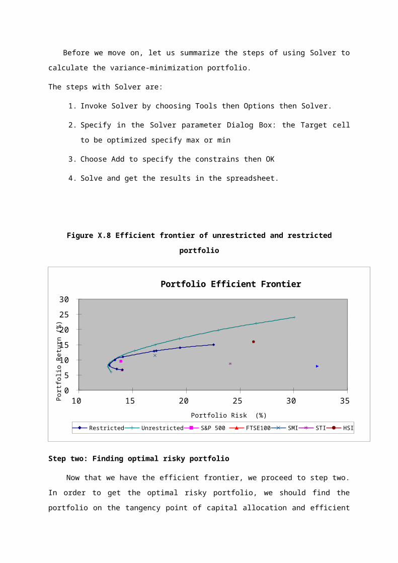
Solver work for you. If you record a sufficient number of points, you will be able to generate a graph

of the quality of Figure X.8.

If short selling is not allowed, the Solver also allows you to all “no short sales” and other

constrains easily. We need to impose the additional constraints that each weight (the elements in

column B and row 49) must be nonnegative. Once they are entered, you repeat the variance-

minimization exercise until you generate the entire restricted frontier. The outer frontier in Figure

X.8 is drawn assuming that the investor may maintain negative portfolio weights, the inside frontier

obtained allowing short sales. Table X.2 E and F present a number of points on the two frontiers with

and without short sales. You can see that the weights in restricted portfolios are never negative. The

minimum variance portfolios in two frontiers are not the same.

Before we move on, let us summarize the steps of using Solver to calculate the variance-

minimization portfolio.

The steps with Solver are:

1. Invoke Solver by choosing Tools then Options then Solver.

2. Specify in the Solver parameter Dialog Box: the Target cell to be optimized specify max or

min

3. Choose Add to specify the constrains then OK

4. Solve and get the results in the spreadsheet.

Figure X.8 Efficient frontier of unrestricted and restricted portfolio

5 If you do not set the second constraint: target mean equal to 20, then you can the minimum variance portfolio. The minimum variance portfolio has 18.637% expected return and a standard deviation of 15.643%.

10 15 20 25 30 35 0

5

10

15

20

25

30

Portfolio Efficient Frontier

Restricted Unrestricted S&P 500 FTSE100 SMI STI HSI

Portfolio Risk (%)

Port

foli

o R

etur

n (%

)

Step two: Finding optimal risky portfolio

Now that we have the efficient frontier, we proceed to step two. In order to get the optimal risky

portfolio, we should find the portfolio on the tangency point of capital allocation and efficient

frontier. To do so, we can use the Solver to help us. First, you enter the of the target function,

“maximum” the reward-to-variability ratio ( ,we assume risk-free rate is 4.01%6) the slope

of the CAL, input the cell range (the portfolio weights, contained in cells B49-B54), and other

necessary constraints( such like the sum of the weights equal to one and others). Then ask the Solver

to find the optimal portfolio weights. The results are shown in Table X.2 E and F. The optimal risky

portfolio with short selling allowance has expected return of 19.784% with a standard deviation of

22.976% (cell B69, C69). The expected return and standard deviation of the restricted optimal risky

portfolio are 12.897%and 16.998% (cell B80, C80).

Step three: Capital allocation decision

One’s allocation decision will influence by his degree of risk aversion. Now we have optimal risky

portfolio, we can use the concept of complete portfolio allocation funds between risky portfolio and

risk-free asset. We use equation X.11 as our utility function and set the risk aversion equal to 5 and

risk-free rate is 4.1%. First we construct a complete portfolio with risk-free asset and optimal risky

portfolio.

6 We use three month Treasury Bill interest rate as the risk-free rate, the average interest rate of 3month T-Bill is 4.09% form 1990/01 to 2006/12.

According to equation X.14, the optimal weight in risky portfolio is and the optimal

position of risk-free asset is 1- . Then we can use equation 5 and 6 calculate the expected

return and standard deviation of the overall optimal portfolio. The results are shown in Table X.2 G

and H. The optimal unrestricted (restricted) portfolio has 13.44% (9.48%) expected return with

13.73% (10.46%) standard deviation. And the investor will invest 60% (62%) of portfolio value in risky

portfolio and 40% (38%) in risk-free asset.

To sum up the three steps, the all results are shown in Table X.3.

Table X.3 The results of optimization problem

portfolio Unrestricted portfolio Restricted portfolio

Minimum variance portfolio

Optimal risky

portfolio

Optimal

Overall portfolio

Minimum variance portfolio

Optimal risky

portfolio

Optimal

Overall portfolio

Portfolio Return

7.73% 19.78% 13.44% 8.28% 12.89% 9.48%

Portfolio Risk

12.71% 22.98% 13.73% 12.83% 16.99% 10.46%