efficient execution of deep neural networks on mobile

Efficient Execution of Deep Neural Networks onMobile Devices with NPU

Tianxiang TanThe Pennsylvania State University

State College, [email protected]

Guohong CaoThe Pennsylvania State University

State College, [email protected]

ABSTRACTMany Deep Neural Network (DNN) based applications havebeen developed and run on mobile devices. Although theseadvanced DNN models can provide better results, they alsosuffer from high computational overhead which means longdelay and more energy consumption when running on mo-bile devices. To address these problems, many companieshave developed dedicated Neural Processing Units (NPUs)for mobile devices, which can process AI features. Comparedto CPU, NPU can run DNN models much faster, but withlower accuracy. To address this issue, we leverage modelpartition techniques to improve the performance of DNNmodels on mobile devices with NPU. The challenge is to de-termine which part of the DNN model should be run on CPUand which part to be run on NPU. Based on the delay andthe accuracy requirements of the applications, we study twoproblems: Max-Accuracy where the goal is to maximize theaccuracy under some time constraint, and Min-Time wherethe goal is to minimize the processing time while ensuringthe accuracy is above a certain threshold. To solve theseproblems, we propose heuristic based algorithms which aresimple but only search a small number of layer combinations(i.e., where to run which DNN model layers). To furtherimprove the performance, we propose a Machine Learningbased Model Partition (MLMP) algorithm. MLMP searchesmore layer combinations and considers both accuracy lossand processing time simultaneously. We also address manyimplementation issues to support model partition techniqueson mobile devices with NPU. Experimental results show thatMLMP outperforms the heuristic based algorithms and it can

Permission to make digital or hard copies of all or part of this work forpersonal or classroom use is granted without fee provided that copies are notmade or distributed for profit or commercial advantage and that copies bearthis notice and the full citation on the first page. Copyrights for componentsof this work owned by others than ACMmust be honored. Abstracting withcredit is permitted. To copy otherwise, or republish, to post on servers or toredistribute to lists, requires prior specific permission and/or a fee. Requestpermissions from [email protected]’ 21, May 18–21, 2021, Nashville, TN, USA© 2021 Association for Computing Machinery.ACM ISBN 978-1-4503-8098-0/21/05. . . $15.00https://doi.org/10.1145/3412382.3458272

significantly improve the accuracy or reduce the processingtime based on the application requirements.

CCS CONCEPTS• Human-centered computing → Ubiquitous and mobilecomputing; •Computingmethodologies→Machine learn-ing; • Computer systems organization → Embedded andcyber-physical systems.

KEYWORDSNPU, Deep Learning, Mobile Computing, Internet of Things

ACM Reference Format:Tianxiang Tan and Guohong Cao. 2021. Efficient Execution of DeepNeural Networks on Mobile Devices with NPU. In InformationProcessing in Sensor Networks (IPSN’ 21), May 18–21, 2021, Nashville,TN, USA. ACM, New York, NY, USA, 16 pages. https://doi.org/10.1145/3412382.3458272

1 INTRODUCTIONDeep neural networks (DNNs) have been successfully ap-plied to various problems in computer vision, natural lan-guage processing, healthcare, etc., and some of the advancedmodels can even outperform human beings in some spe-cific datasets [29, 46]. Recently, many applications based onDNN models have been developed and run on mobile de-vices. For example, DNN based apps can recognize user’svoice as text input [4, 33], assist travelers identify buildingsand landmarks [41, 42], and detect Parkinson’s disease byanalyzing users’ vocal sound [53]. Although these advancedDNN models can provide us with better results, they alsosuffer from the high computational overhead which meanslong delay and more energy consumption when running onmobile devices.

To address these problems, mobile devices can offload com-putationally intensive applications to the cloud. Althoughoffloading techniques can reduce the computation time, itmay take much longer time to transmit data, especially whenthere is limited wireless bandwidth, or when the data sizeis large which is usually true for applications using DNNs.Moreover, there are other issues such as the lack of serversupport or privacy concerns. For example, some users prefer

https://doi.org/10.1145/3412382.3458272

https://doi.org/10.1145/3412382.3458272

https://doi.org/10.1145/3412382.3458272

IPSN’ 21, May 18–21, 2021, Nashville, TN, USA Tianxiang Tan and Guohong Cao

processing sensitive data locally, even though the processingtime is much longer.

To efficiently execute the DNN models locally, many com-panies such as Huawei, Qualcomm, and Samsung have de-veloped dedicated Neural Processing Units (NPUs) for mobiledevices, which can process AI features. With NPU, the run-ning time of these DNN models can be significantly reduced.For example, on HUAWEI mate 10 pro, running ResNet-50(a DNN model) [16] on NPU is 20 times faster than runningit on CPU. Although NPUs are only available on advancedphone models at this time, it has great potential to be appliedto other mobile devices and even IoT devices in the nearfuture. For example, the Qualcomm Snapdragon 855 [36] hasa NPU chipset dedicated for AI and Samsung has committedto increase the number of employees working on NPU tech-nologies by ten times in the next decade [40]. HUAWEI hasalready deployed NPU on its current and future smartphonemodels such as Mate 30 pro and Nova series [20].

There are some fundamental limitations with NPU whichpose research challenges for efficiently and effectively exe-cuting DNN models on NPU. The most significant limitationof NPU is the precision of the floating-point numbers. NPUuses 16 bits or 8 bits to represent the floating-point numbersinstead of 32 bits in CPU. As a result, it runs DNN modelsmuch faster but less accurate compared to CPU, and it is achallenge to improve the accuracy of running DNN modelson NPU.

To address this problem, we leverage model partition tech-niques to improve the performance of DNN models on mo-bile devices with NPU. Model partition techniques have beenstudied in [17, 22, 30, 44], where the DNN model is splitinto different layers and executed in different places, such asCPU, GPU or cloud server. However, their focus is to reducethe computation time, and none of them considers the lowaccuracy problem introduced by NPU.The major challenge of applying model partition tech-

niques is to determine which layers are run on CPU andwhich layers are run on NPU, based on the processing timeand the accuracy requirement of the application. Consideran example of a flying drone. The camera on the drone takesvideos which are processed in real time to detect nearbyobjects to avoid crashing into a building or being trappedby a tree. To ensure no object is missed, the detection resultshould be as accurate as possible. Here, the time constraintis critical, and we should maximize the accuracy under sometime constraint. For other applications, such as unlocking asmartphone, making payment through face recognition, theaccuracy is more important than the processing time. Hence,we should minimize the processing time while ensuring thatthe accuracy is above a certain threshold.

Based on the processing time and accuracy requirement ofdifferent mobile applications, we study two problems: Max-Accuracy where the goal is to maximize the accuracy undersome time constraints and Min-Time where the goal is tominimize the processing time while ensuring the accuracyis above a certain threshold.Different DNN model layers perform different floating-

point operations, and hence they have different characteris-tics in terms of processing time and accuracy when being runon NPU or CPU. Some layers are sensitive to low precisionfloating-point operations on NPU and running them on NPUwill result in lower accuracy. Some other layers are compu-tationally intensive and running them on CPU will resultin longer processing time. In this paper, we identify thesespecial characteristics of running DNN models on mobiledevices with NPU. We formalize the Max-accuracy prob-lem and the Min-Time problem, and then propose heuristicbased solutions to solve them based on the identified specialcharacteristics. More specifically, we propose model parti-tion techniques to determine which layers to run on CPUand which layers to run on NPU to satisfy the applicationrequirements on delay and accuracy.Since our heuristic based solutions only try a small num-

ber of layer combinations (i.e., where to run which layer),we further improve the performance by proposing a Ma-chine Learning based Model Partition (MLMP) algorithm.MLMP tries more layer combinations and considers bothaccuracy loss and processing time simultaneously. It lever-ages machine learning techniques to efficiently estimate theaccuracy loss of running the DNN models with a layer com-bination. Since the Software Develop Kit (SDK) for NPU doesnot include tools to measure the layer processing time onNPU, and the data transmission time between NPU andmem-ory, we also propose techniques to better estimate them, andthen determine how to partition model layers between CPUand NPU for Max-accuracy or Min-Time.

Our contributions are summarized as follows.

• We identify some special characteristics of runningDNN models on NPU to help determine where to runwhich layers to achieve better tradeoffs between accu-racy and delay.• We formulate theMax-Accuracy problem and theMin-Time problem, and propose heuristic based algorithmsto solve them.• To address the limitations of the heuristic based algo-rithms, we propose a machine learning based modelpartition (MLMP) algorithm to further improve theperformance.• We address many implementation issues on achievingmodel partition onmobile devices with NPU. Extensiveevaluation results show that MLMP can significantly

Efficient Execution of Deep Neural Networks on Mobile Devices with NPU IPSN’ 21, May 18–21, 2021, Nashville, TN, USA

improve the accuracy or reduce the processing timebased on the application requirements.

The rest of the paper is organized as follows. Section 2presents the special characteristics of running DNN mod-els on NPU. In Section 3, we formalize the Max-Accuracyproblem and the Min-Time problem, and propose heuristicalgorithms to solve them. Section 4 presents the technicaldetails of MLMP. Section 5 presents implementation detailsof our algorithms and Section 6 shows the evaluation results.Section 7 presents related work and Section 8 concludes thepaper.

2 PRELIMINARYIn this section, we first use some measurement results toshow the special characteristics of NPU, and then give themotivation of using model partition techniques to improvethe performance.

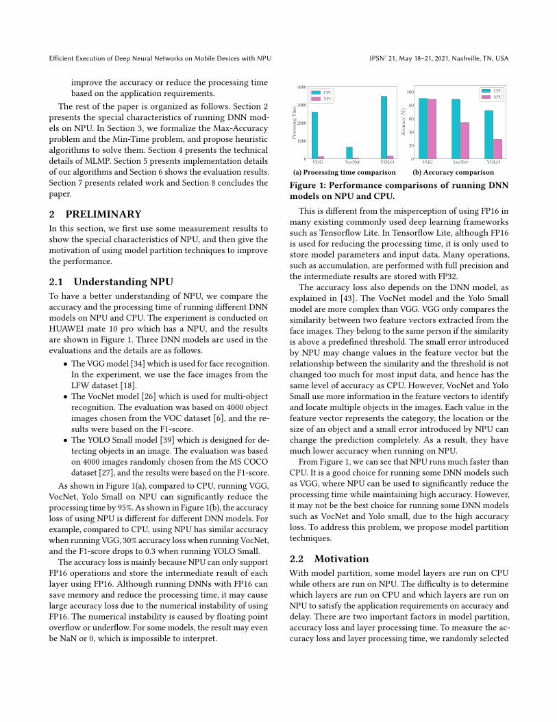
2.1 Understanding NPUTo have a better understanding of NPU, we compare theaccuracy and the processing time of running different DNNmodels on NPU and CPU. The experiment is conducted onHUAWEI mate 10 pro which has a NPU, and the resultsare shown in Figure 1. Three DNN models are used in theevaluations and the details are as follows.• The VGGmodel [34] which is used for face recognition.In the experiment, we use the face images from theLFW dataset [18].• The VocNet model [26] which is used for multi-objectrecognition. The evaluation was based on 4000 objectimages chosen from the VOC dataset [6], and the re-sults were based on the F1-score.• The YOLO Small model [39] which is designed for de-tecting objects in an image. The evaluation was basedon 4000 images randomly chosen from the MS COCOdataset [27], and the results were based on the F1-score.

As shown in Figure 1(a), compared to CPU, running VGG,VocNet, Yolo Small on NPU can significantly reduce theprocessing time by 95%. As shown in Figure 1(b), the accuracyloss of using NPU is different for different DNN models. Forexample, compared to CPU, using NPU has similar accuracywhen running VGG, 30% accuracy loss when running VocNet,and the F1-score drops to 0.3 when running YOLO Small.

The accuracy loss is mainly because NPU can only supportFP16 operations and store the intermediate result of eachlayer using FP16. Although running DNNs with FP16 cansave memory and reduce the processing time, it may causelarge accuracy loss due to the numerical instability of usingFP16. The numerical instability is caused by floating pointoverflow or underflow. For some models, the result may evenbe NaN or 0, which is impossible to interpret.

VGG VocNet YOLO0

1000

2000

3000

4000

Pro

cess

ing

Tim

e

CPU

NPU

(a) Processing time comparisonVGG VocNet YOLO

0

20

40

60

80

100

Acc

ura

cy(%

)

CPU

NPU

(b) Accuracy comparison

Figure 1: Performance comparisons of running DNNmodels on NPU and CPU.

This is different from the misperception of using FP16 inmany existing commonly used deep learning frameworkssuch as Tensorflow Lite. In Tensorflow Lite, although FP16is used for reducing the processing time, it is only used tostore model parameters and input data. Many operations,such as accumulation, are performed with full precision andthe intermediate results are stored with FP32.The accuracy loss also depends on the DNN model, as

explained in [43]. The VocNet model and the Yolo Smallmodel are more complex than VGG. VGG only compares thesimilarity between two feature vectors extracted from theface images. They belong to the same person if the similarityis above a predefined threshold. The small error introducedby NPU may change values in the feature vector but therelationship between the similarity and the threshold is notchanged too much for most input data, and hence has thesame level of accuracy as CPU. However, VocNet and YoloSmall use more information in the feature vectors to identifyand locate multiple objects in the images. Each value in thefeature vector represents the category, the location or thesize of an object and a small error introduced by NPU canchange the prediction completely. As a result, they havemuch lower accuracy when running on NPU.

From Figure 1, we can see that NPU runs much faster thanCPU. It is a good choice for running some DNN models suchas VGG, where NPU can be used to significantly reduce theprocessing time while maintaining high accuracy. However,it may not be the best choice for running some DNN modelssuch as VocNet and Yolo small, due to the high accuracyloss. To address this problem, we propose model partitiontechniques.

2.2 MotivationWith model partition, some model layers are run on CPUwhile others are run on NPU. The difficulty is to determinewhich layers are run on CPU and which layers are run onNPU to satisfy the application requirements on accuracy anddelay. There are two important factors in model partition,accuracy loss and layer processing time. To measure the ac-curacy loss and layer processing time, we randomly selected


C1 P1 C2 P2 C3 C4 C5 C6 P6 C7 C8 C9 C10 C11 C12 C13 C14 C15 C16 P16 C17 C18 C19 C20 C21 C22 C23 C24 F25 F26 F27

Layer

0.00

0.02

0.04

0.06

0.08

0.10

Pro

cess

ing

Tim

eR

edu

ctio

n

0.0

0.1

0.2

0.3

0.4

0.5

0.6

Acc

ura

cyL

oss

Processing Time Reduction

Accuracy Loss

Figure 2: Processing time reduction and accuracy loss for running each layer of Yolo Small on NPU (C: convolu-tional layer, P: pooling layer, F: fully connected layer).

4000 images from the MS COCO dataset and used YOLOSmall (a DNN model) to detect objects with a HUAWEI mate10 pro.

Figure 2 shows the processing time reduction and the ac-curacy loss by running each layer in the Yolo Small modelon NPU. For example, running layer 𝑃2 on NPU while otherlayers are run on CPU can reduce the processing time by6% and incur 4% accuracy loss. Intuitively, a layer (e.g., 𝐶6)should be run on NPU if the processing time can be signifi-cantly reduced with little or no accuracy loss. A layer (e.g.,𝐶17) should be run on CPU if running it on NPU has muchhigher accuracy loss but little processing time reduction.However, most of the layers (e.g., 𝐶23) are not under thesetwo extreme cases, and hence it is hard to determine whereto run these layers. When considering the overlap effectsof running multiple layers, the decision will be harder. Forexample, the accuracy loss of running 𝐶6 and 𝐶22 on NPUwhile other layers on CPU is 0.08 which is not equivalent tothe sum of their accuracy loss (i.e., 0.04). The accuracy loss ofrunning the DNNwith a layer combination depends onmanyfactors, such as the number of additions and multiplicationsperformed in each layer and the memory space occupied bythe input/output data. Due to complex relationship betweenthe accuracy loss and these factors, it is difficult to derivean equation to estimate the accuracy of running the DNNmodel with a layer combination.

For a DNN model with 𝑛 layers, there are 2𝑛 model parti-tion decisions. For an advanced DNNmodel, there are usuallydozens or even hundreds of layers and hence it is impossibleto use brute force methods to find the best solution. To ad-dress this issue, we first formulate the Max-Accuracy and theMin-Time problem and propose heuristic based algorithmsto solve them. Then, we propose a machine learning basedmodel partition (MLMP) algorithm to further improve theperformance.

Notation Description𝑛 The number of layers in the DNN model𝑙𝑖 The 𝑖𝑡ℎ layer in the DNN model𝐿 A layer combination

𝐴(𝐿) The accuracy of running DNN model with 𝐿𝑇 (𝐿) The processing time of running DNN with 𝐿\𝑡 The time constraint of the application\𝑎 The accuracy requirement the application

Table 1: Notation.

3 MAX-ACCURACY AND MIN-TIMEBased on the processing time and accuracy requirement ofdifferent mobile applications, we study two problems in thissection: Max-Accuracy where the goal is to maximize theaccuracy under some time constraints and Min-Time wherethe goal is to minimize the time while ensuring the accuracyis above a certain threshold.

3.1 The Max-Accuracy ProblemIn the scenario described in the introduction, the processingtime is significant for some applications such as the flyingdrone, and we should maximize the accuracy under sometime constraints; i.e., the Max-Accuracy problem. In thissubsection, we first formulate the problem and then proposea heuristic based solution.Let 𝐿 denote a layer combination and 𝐿 is a list of binary

variables 𝑥𝑖 (𝐿 = (𝑥1, 𝑥2, . . . , 𝑥𝐿)), which indicates whetherthe 𝑖𝑡ℎ layer 𝑙𝑖 will be run on the NPU. More specifically, if𝑥𝑖 = 1, layer 𝑙𝑖 will be run on NPU; if 𝑥𝑖 = 0, layer 𝑙𝑖 willbe run on CPU. Let 𝐴(𝐿) denote the accuracy of runningthe DNN model with a layer combination 𝐿. Let𝑇 (𝐿) denotethe data processing time of running the DNN model with alayer combination 𝐿 and the time constraint for the mobileapplication is \𝑡 . Then, we have 𝑇 (𝐿) = 𝑇 (𝑥1, 𝑥2, . . . , 𝑥𝑛) ≤\𝑡 , and the Max-Accuracy problem can be formulated asfollow.


max 𝐴(𝑥1, 𝑥2, . . . , 𝑥𝑛)s.t. 𝑇 (𝑥1, 𝑥2, . . . , 𝑥𝑛) ≤ \𝑡

𝑥𝑖 ∈ {0, 1},∀𝑖 ∈ [1, 𝑛]A brute force method to solve the Max-Accuracy problem

is to try all possible layer combinations, and it takes 𝑂 (2𝑛).Since the brute force method is impractical, we propose aheuristic based solution, called the Max-Accuracy algorithm.The basic idea is to move layers with higher accuracy lossfrom NPU to CPU since it is the most effective way to im-prove the accuracy. More specifically, our Max-Accuracyalgorithm can be summarized as follows.(1) Initially, all layers are run on NPU.(2) Sort the layers in the descending order based on their

accuracy loss.(3) Starting from the first layer, move the layer from NPU

toCPUuntil the processing time constraint is no longersatisfied. Note that the last layer will not really bemoved from NPU to CPU to ensure that the process-ing time constraint is satisfied.

In the algorithm, the accuracy and the processing time ofrunning DNN models with a layer combination is measuredthrough experiments. Since there are 𝑛 layers in a DNNmodel, the Max-Accuracy algorithm has a time complexityof 𝑂 (𝑛).

3.2 The Min-Time ProblemFor applications such as unlocking a smartphone, makingpayment through face recognition, accuracy is more impor-tant than the processing time. Hence, we study the Min-Timeproblem in this subsection, where the goal is to minimize thetime while ensuring the accuracy is above a certain threshold.We first formulate the problem and then propose a heuristicbased solution.

Let \𝑎 denote the accuracy requirement of the application.For a layer combination𝐿, we have𝐴(𝐿) = 𝐴(𝑥1, 𝑥2, . . . , 𝑥𝑛) ≥\𝑎 . The Min-Time problem can be formulated as follow.

min 𝑇 (𝑥1, 𝑥2, . . . , 𝑥𝑛)s.t. 𝐴(𝑥1, 𝑥2, . . . , 𝑥𝑛) ≥ \𝑎

𝑥𝑖 ∈ {0, 1},∀𝑖 ∈ [1, 𝑛]As mentioned in the Max-Accuracy Algorithm, it is im-

practical to use the brute force method to solve the Min-Timeproblem. Therefore, we propose a heuristic based solution,called the Min-Time Algorithm. The basic idea is to movelayers with longer processing time from CPU to NPU since itis the most effective way to reduce the processing time. Morespecifically, our Min-Time algorithm can be summarized asfollows.

(1) Initially, all layers are run on CPU.(2) Sort the layers in the descending order based on their

processing time.(3) Starting from the first layer, move the layer from CPU

to NPU until the accuracy requirement is no longersatisfied. Note that the last layer will not really bemoved from CPU to NPU to ensure that the accuracyrequirement is satisfied.

Like the Max-Accuracy algorithm, the Min-Time algo-rithm can be easily implemented, and it has a low time com-plexity of 𝑂 (𝑛).

4 MACHINE LEARNING BASED MODELPARTITION (MLMP)

4.1 OverviewBy leveragingmodel partition techniques, Max-Accuracy cansignificantly improve the accuracy compared to running allDNN layers on NPU, and Min-Time can significantly reducethe processing time compared to running all DNN layerson CPU. However, both approaches have limitations, for ex-ample, they only try a small number of layer combinationsbased on heuristics, and better solutions may exist. Moreover,some factors are not considered to simplify the problem. Forexample, two layers with similar accuracy loss may havedifferent processing time and moving any one of them fromNPU to CPU leads to similar accuracy improvement. How-ever, Max-Accuracy does not consider such difference, andthen the processing time will increase significantly if thelayer with longer processing time is moved from NPU toCPU.

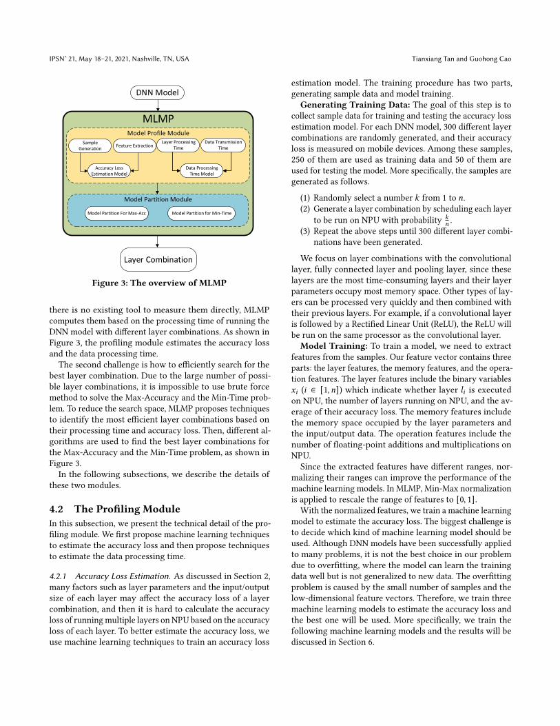
To address these limitations, we propose a machine learn-ing based model partition (MLMP) algorithm which triesmore layer combinations and considers both accuracy lossand processing time simultaneously. Figure 3 shows theoverview of MLMP. MLMP has two main modules: the profil-ing module and the model partition module, which addressthe following two challenges.The first challenges is how to estimate the accuracy and

processing time efficiently when there are a large number oflayer combinations. In Max-Acc and Min-Time, we measurethe accuracy and the processing time by running DNNmodelwith different layer combinations on smartphones. However,such measurement is very time consuming since it needs toprocess all data in the dataset. It is also impractical whenthere are many layer combinations to be measured. MLMPleverages machine learning techniques to efficiently estimatethe accuracy loss of running DNN models with a layer com-bination. To estimate the data processing time of runningthe DNN model with a layer combination, MLMP needs toknow the layer processing time on NPU and the data trans-mission time between CPU and NPU for each layer. Since


Layer Combination

MLMP

DNN Model

Data Transmission Time

Layer Processing TimeFeature Extraction

Accuracy Loss Estimation Model

Data Processing Time Model

Model Profile Module

Sample Generation

Model Partition Module

Model Partition For Max-Acc Model Partition for Min-Time

Figure 3: The overview of MLMP

there is no existing tool to measure them directly, MLMPcomputes them based on the processing time of running theDNN model with different layer combinations. As shown inFigure 3, the profiling module estimates the accuracy lossand the data processing time.The second challenge is how to efficiently search for the

best layer combination. Due to the large number of possi-ble layer combinations, it is impossible to use brute forcemethod to solve the Max-Accuracy and the Min-Time prob-lem. To reduce the search space, MLMP proposes techniquesto identify the most efficient layer combinations based ontheir processing time and accuracy loss. Then, different al-gorithms are used to find the best layer combinations forthe Max-Accuracy and the Min-Time problem, as shown inFigure 3.In the following subsections, we describe the details of

these two modules.

4.2 The Profiling ModuleIn this subsection, we present the technical detail of the pro-filing module. We first propose machine learning techniquesto estimate the accuracy loss and then propose techniquesto estimate the data processing time.

4.2.1 Accuracy Loss Estimation. As discussed in Section 2,many factors such as layer parameters and the input/outputsize of each layer may affect the accuracy loss of a layercombination, and then it is hard to calculate the accuracyloss of runningmultiple layers on NPU based on the accuracyloss of each layer. To better estimate the accuracy loss, weuse machine learning techniques to train an accuracy loss

estimation model. The training procedure has two parts,generating sample data and model training.

Generating Training Data: The goal of this step is tocollect sample data for training and testing the accuracy lossestimation model. For each DNN model, 300 different layercombinations are randomly generated, and their accuracyloss is measured on mobile devices. Among these samples,250 of them are used as training data and 50 of them areused for testing the model. More specifically, the samples aregenerated as follows.

(1) Randomly select a number 𝑘 from 1 to 𝑛.(2) Generate a layer combination by scheduling each layer

to be run on NPU with probability 𝑘𝑛.

(3) Repeat the above steps until 300 different layer combi-nations have been generated.

We focus on layer combinations with the convolutionallayer, fully connected layer and pooling layer, since theselayers are the most time-consuming layers and their layerparameters occupy most memory space. Other types of lay-ers can be processed very quickly and then combined withtheir previous layers. For example, if a convolutional layeris followed by a Rectified Linear Unit (ReLU), the ReLU willbe run on the same processor as the convolutional layer.

Model Training: To train a model, we need to extractfeatures from the samples. Our feature vector contains threeparts: the layer features, the memory features, and the opera-tion features. The layer features include the binary variables𝑥𝑖 (𝑖 ∈ [1, 𝑛]) which indicate whether layer 𝑙𝑖 is executedon NPU, the number of layers running on NPU, and the av-erage of their accuracy loss. The memory features includethe memory space occupied by the layer parameters andthe input/output data. The operation features include thenumber of floating-point additions and multiplications onNPU.Since the extracted features have different ranges, nor-

malizing their ranges can improve the performance of themachine learning models. In MLMP, Min-Max normalizationis applied to rescale the range of features to [0, 1].

With the normalized features, we train a machine learningmodel to estimate the accuracy loss. The biggest challenge isto decide which kind of machine learning model should beused. Although DNN models have been successfully appliedto many problems, it is not the best choice in our problemdue to overfitting, where the model can learn the trainingdata well but is not generalized to new data. The overfittingproblem is caused by the small number of samples and thelow-dimensional feature vectors. Therefore, we train threemachine learning models to estimate the accuracy loss andthe best one will be used. More specifically, we train thefollowing machine learning models and the results will bediscussed in Section 6.


Linear RegressionThismachine learning technique is widelyused in predictive analysis. It models the relationship be-tween accuracy loss and our extracted features using a linearequation. In MLMP, ridge regression is used to prevent over-fitting.

Multilayer Perceptron Neural Network (MLP):MLP is a classof feedforward neural network models. It has high capacityand is widely used for classification or regression problems.In MLMP, we build a two-layer fully connected neural net-work and use LeRU as the activation function. Each hiddenlayer in the model includes dozens of neurons and L2 regu-larization is used to prevent overfitting.

Gradient Boosting Regression Tree (GBRT): GBRT is an en-semble machine learning model for regression problems. Ittrains several regression tree models sequentially. For eachregression tree model, it optimizes the loss function and cor-rect the errors made by the previous trained regression treemodels.

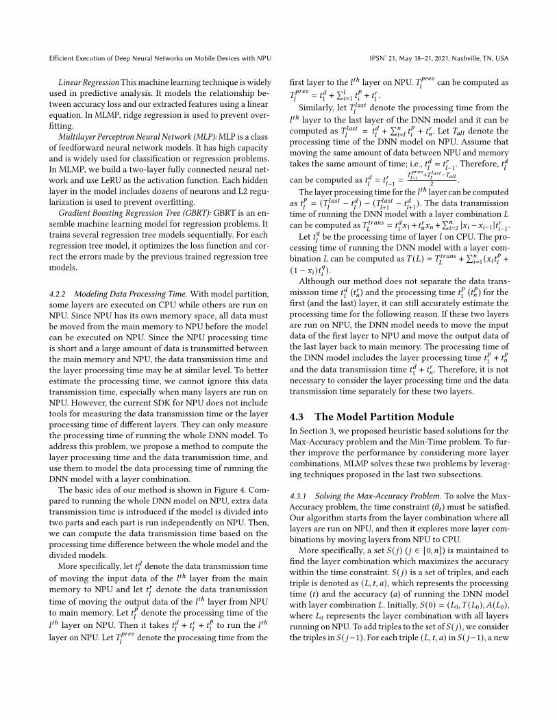
4.2.2 Modeling Data Processing Time. With model partition,some layers are executed on CPU while others are run onNPU. Since NPU has its own memory space, all data mustbe moved from the main memory to NPU before the modelcan be executed on NPU. Since the NPU processing timeis short and a large amount of data is transmitted betweenthe main memory and NPU, the data transmission time andthe layer processing time may be at similar level. To betterestimate the processing time, we cannot ignore this datatransmission time, especially when many layers are run onNPU. However, the current SDK for NPU does not includetools for measuring the data transmission time or the layerprocessing time of different layers. They can only measurethe processing time of running the whole DNN model. Toaddress this problem, we propose a method to compute thelayer processing time and the data transmission time, anduse them to model the data processing time of running theDNN model with a layer combination.The basic idea of our method is shown in Figure 4. Com-

pared to running the whole DNN model on NPU, extra datatransmission time is introduced if the model is divided intotwo parts and each part is run independently on NPU. Then,we can compute the data transmission time based on theprocessing time difference between the whole model and thedivided models.

More specifically, let 𝑡𝑑𝑙denote the data transmission time

of moving the input data of the 𝑙𝑡ℎ layer from the mainmemory to NPU and let 𝑡𝑟

𝑙denote the data transmission

time of moving the output data of the 𝑙𝑡ℎ layer from NPUto main memory. Let 𝑡𝑝

𝑙denote the processing time of the

𝑙𝑡ℎ layer on NPU. Then it takes 𝑡𝑑𝑙+ 𝑡𝑟

𝑙+ 𝑡𝑝

𝑙to run the 𝑙𝑡ℎ

layer on NPU. Let𝑇 𝑝𝑟𝑒𝑣

𝑙denote the processing time from the

first layer to the 𝑙𝑡ℎ layer on NPU. 𝑇 𝑝𝑟𝑒𝑣

𝑙can be computed as

𝑇𝑝𝑟𝑒𝑣

𝑙= 𝑡𝑑1 +

∑𝑙𝑖=1 𝑡

𝑝

𝑖+ 𝑡𝑟

𝑙.

Similarly, let 𝑇 𝑙𝑎𝑠𝑡𝑙

denote the processing time from the𝑙𝑡ℎ layer to the last layer of the DNN model and it can becomputed as 𝑇 𝑙𝑎𝑠𝑡

𝑙= 𝑡𝑑

𝑙+ ∑𝑛

𝑖=𝑙𝑡𝑝

𝑖+ 𝑡𝑟𝑛 . Let 𝑇𝑎𝑙𝑙 denote the

processing time of the DNN model on NPU. Assume thatmoving the same amount of data between NPU and memorytakes the same amount of time; i.e., 𝑡𝑑

𝑙= 𝑡𝑟

𝑙−1. Therefore, 𝑡𝑑𝑙

can be computed as 𝑡𝑑𝑙= 𝑡𝑟

𝑙−1 =𝑇𝑝𝑟𝑒𝑣

𝑙−1 +𝑇𝑙𝑎𝑠𝑡𝑙−𝑇𝑎𝑙𝑙

2 .The layer processing time for the 𝑙𝑡ℎ layer can be computed

as 𝑡𝑝𝑙= (𝑇 𝑙𝑎𝑠𝑡

𝑙− 𝑡𝑑

𝑙) − (𝑇 𝑙𝑎𝑠𝑡

𝑙+1 − 𝑡𝑑𝑙+1). The data transmission

time of running the DNN model with a layer combination 𝐿can be computed as𝑇 𝑡𝑟𝑎𝑛𝑠

𝐿= 𝑡𝑑1 𝑥1 + 𝑡𝑟𝑛𝑥𝑛 +

∑𝑛𝑖=2 |𝑥𝑖 −𝑥𝑖−1 |𝑡𝑟𝑖−1.

Let 𝑡𝑞𝑙be the processing time of layer 𝑙 on CPU. The pro-

cessing time of running the DNN model with a layer com-bination 𝐿 can be computed as 𝑇 (𝐿) = 𝑇 𝑡𝑟𝑎𝑛𝑠

𝐿+∑𝑛

𝑖=1 (𝑥𝑖𝑡𝑝

𝑖+

(1 − 𝑥𝑖 )𝑡𝑞𝑖 ).Although our method does not separate the data trans-

mission time 𝑡𝑑1 (𝑡𝑟𝑛) and the processing time 𝑡𝑝1 (𝑡𝑝𝑛 ) for thefirst (and the last) layer, it can still accurately estimate theprocessing time for the following reason. If these two layersare run on NPU, the DNN model needs to move the inputdata of the first layer to NPU and move the output data ofthe last layer back to main memory. The processing time ofthe DNN model includes the layer processing time 𝑡𝑝1 + 𝑡

𝑝𝑛

and the data transmission time 𝑡𝑑1 + 𝑡𝑟𝑛 . Therefore, it is notnecessary to consider the layer processing time and the datatransmission time separately for these two layers.

4.3 The Model Partition ModuleIn Section 3, we proposed heuristic based solutions for theMax-Accuracy problem and the Min-Time problem. To fur-ther improve the performance by considering more layercombinations, MLMP solves these two problems by leverag-ing techniques proposed in the last two subsections.

4.3.1 Solving the Max-Accuracy Problem. To solve the Max-Accuracy problem, the time constraint (\𝑡 ) must be satisfied.Our algorithm starts from the layer combination where alllayers are run on NPU, and then it explores more layer com-binations by moving layers from NPU to CPU.More specifically, a set 𝑆 ( 𝑗) ( 𝑗 ∈ [0, 𝑛]) is maintained to

find the layer combination which maximizes the accuracywithin the time constraint. 𝑆 ( 𝑗) is a set of triples, and eachtriple is denoted as (𝐿, 𝑡, 𝑎), which represents the processingtime (𝑡 ) and the accuracy (𝑎) of running the DNN modelwith layer combination 𝐿. Initially, 𝑆 (0) = (𝐿0,𝑇 (𝐿0), 𝐴(𝐿0),where 𝐿0 represents the layer combination with all layersrunning on NPU. To add triples to the set of 𝑆 ( 𝑗), we considerthe triples in 𝑆 ( 𝑗−1). For each triple (𝐿, 𝑡, 𝑎) in 𝑆 ( 𝑗−1), a new


Intermediate

Data Output

Layer Layer Layer Layer

Figure 4: Modeling the data processing time of running the DNN model with a layer combination.

layer combination 𝐿′ is generated by moving a layer runningon NPU in 𝐿 to CPU. Since the time constraint must be satis-fied for the layer combinations, the tuple (𝐿′,𝑇 (𝐿′), 𝐴(𝐿′))is added to 𝑆 ( 𝑗) if and only if 𝑇 (𝐿′) ≤ \𝑡 .

Not all possible triples are maintained in 𝑆 ( 𝑗), since onlythe most efficient ones (i.e., with higher accuracy and lessprocessing time) are kept. More specifically, a triple (𝐿, 𝑡, 𝑎)is said to dominate another triple (𝐿′, 𝑡 ′, 𝑎′) if and only if𝑡 ≤ 𝑡 ′, 𝑎 ≥ 𝑎′. The layer combination 𝐿 is more efficient thanthe layer combination 𝐿′ and all dominated triples will beremoved from the list of 𝑆 ( 𝑗).The number of layer combinations in 𝑆 ( 𝑗) may quickly

grow as 𝑗 increases. To improve the search efficiency, MLMPuses a predefined threshold 𝐾 to limit the number of triplesin 𝑆 ( 𝑗). More specifically, the triples in 𝑆 ( 𝑗) are sorted in thedescending order of their accuracy and 𝑆 ( 𝑗) only keeps thefirst 𝐾 triples.

Themodel partition algorithm is summarized inAlgorithm1. In the algorithm, 𝐴𝑏𝑒𝑠𝑡 is used for tracking the maximumaccuracy that has been found so far, and its correspondinglayer combination is maintained by 𝐿𝑏𝑒𝑠𝑡 .

4.3.2 Solving the Min-Time Problem. To solve the Min-Timeproblem, the accuracy requirement (\𝑎) must be satisfied. Ouralgorithm starts from the layer combination where all layersare run onCPU, and then it exploresmore layer combinationsby moving layers from CPU to NPU.The algorithm is similar to the Algorithm 1 and the key

difference is that the accuracy requirement must be satisfiedfor all layer combinations in 𝑆 ( 𝑗) ( 𝑗 ∈ [0, 𝑛]). More specifi-cally, the set 𝑆 (0) = {𝐿′0,𝑇 (𝐿′0), 𝐴(𝐿′0)}, where 𝐿′0 is the layercombinations where all layers are run on CPU. 𝐴(𝐿) ≥ \𝑎must be satisfied when a triple (𝐿,𝑇 (𝐿), 𝐴(𝐿)) is added to𝑆 ( 𝑗). The techniques for improving the search efficiency inAlgorithm 1 is also applied to 𝑆 ( 𝑗).

The model partition algorithm is summarized in Algo-rithm 2. In the algorithm, 𝑇𝑏𝑒𝑠𝑡 is used for tracking the mini-mum data processing time that has been found so far, andits corresponding layer combination is maintained by 𝐿𝑏𝑒𝑠𝑡 .

Algorithm 1: Solving Max-Acc with MLMPResult: The layer combination 𝐿𝑏𝑒𝑠𝑡 which

maximizes the accuracy1 𝑆 (0) ← {(𝐿0,𝑇 (𝐿0), 𝐴(𝐿0)},

𝐴𝑏𝑒𝑠𝑡 ← 𝐴(𝐿0), 𝐿𝑏𝑒𝑠𝑡 ← 𝐿02 for 𝑗 from 1 to 𝑛 do3 for each (𝐿, 𝑡, 𝑎) in 𝑆 ( 𝑗 − 1) do4 for each layer that is run on NPU in 𝐿 do5 Generate 𝐿′ by moving the layer from

NPU to CPU in 𝐿.6 if 𝑇 (𝐿′) ≤ \𝑡 then7 Add (𝐿′,𝑇 (𝐿′), 𝐴(𝐿′)) to 𝑆 ( 𝑗)8 if 𝐴𝑏𝑒𝑠𝑡 < 𝐴(𝐿′) then9 𝐴𝑏𝑒𝑠𝑡 ← 𝐴(𝐿′), 𝐿𝑏𝑒𝑠𝑡 ← 𝐿′

10 Remove the dominated triples from 𝑆 ( 𝑗).11 Sort the triples in 𝑆 ( 𝑗) in the descending

order of their accuracy.12 𝑆 ( 𝑗) keeps the first 𝐾 triples and remove

others.13 Return 𝐿𝑏𝑒𝑠𝑡

5 IMPLEMENTATIONSFigure 5 shows the details of our implementation which isdivided into two parts: one runs on the server and the otherone runs on the mobile device. For a DNN model, the serverfinds the layer combination based on the Max-Accuracy al-gorithm, the Min-Time algorithm, or the MLMP algorithm.The result will be sent to the mobile device. Note that theproposed algorithms only need to run once for a particu-lar DNN model or a particular application requirement. Aslong as the DNN model and the application requirementsare not changed, the mobile device can keep using the layercombination.Since Max-Accuracy and Min-Time are simple, no addi-

tional library is needed for implementation. However, theMLMP algorithm is more complex, where machine learningmodels are trained to estimate the accuracy loss. We train


Algorithm 2: Solving Min-Time with MLMPResult: The layer combination 𝐿𝑏𝑒𝑠𝑡 which

minimizes the data processing time1 𝑆 (0) ← {(𝐿′0,𝑇 (𝐿′0), 𝐴(𝐿′0)},

𝑇𝑏𝑒𝑠𝑡 ← 𝑇 (𝐿′0), 𝐿𝑏𝑒𝑠𝑡 ← 𝐿′02 for 𝑗 from 1 to 𝑛 do3 for each (𝐿, 𝑡, 𝑎) in 𝑆 ( 𝑗 − 1) do4 for each layer that is run on CPU in 𝐿 do5 Generate 𝐿′ by moving the layer from

CPU to NPU in 𝐿.6 if 𝐴(𝐿′) ≥ \𝑎 then7 Add (𝐿′,𝑇 (𝐿′), 𝐴(𝐿′)) to 𝑆 ( 𝑗)8 if 𝑇𝑏𝑒𝑠𝑡 > 𝑇 (𝐿′) then9 𝑇𝑏𝑒𝑠𝑡 ← 𝑇 (𝐿′), 𝐿𝑏𝑒𝑠𝑡 ← 𝐿′

10 Remove the dominated triples from 𝑆 ( 𝑗).11 Sort the triples in 𝑆 ( 𝑗) in the ascending order

of their data processing time.12 𝑆 ( 𝑗) keeps the first 𝐾 triples and remove

others.13 Return 𝐿𝑏𝑒𝑠𝑡

DNN Models

……

Scikit-Learn

JNI functions

Caffe Library

JavaCV

CPU NPU

Mobile Device

CPU NPU

Mobile Device

ServerServer

Input Data

NPU Model Optimizer

NPU SDK

Partitioned DNN ModelsPartitioned DNN Models

…

Min-Time MLMPMax-Acc Min-Time MLMPMax-Acc

Figure 5: The implementation details

these models using the Scikit-learn library [35]. Althoughthe library has already included API for building up the mod-els, there are many parameters to be determined. We usethe gird search method to optimize the parameters for eachmodel.

After finding out a layer combination, the partitionedDNNmodels should be optimized before running on NPU sinceNPU has a different architecture from CPU. The HUAWEIDDK includes toolsets to perform such optimizations forDNN models trained by deep learning frameworks such asCaffe [23] or Tensorflow.To run the partitioned DNN models on CPU, we use the

Caffe deep learning framework. Since the HUAWEI mate 10pro uses Android system, we cross-compile the Caffe frame-work using NDK [11]. Although there is an existing Android

Caffe library, it only has limited functions and cannot exe-cute a set of specific layers on CPU. Therefore, we add morefunctions to the existing library and cross-compile it to theAndroid platform.

To run DNN model layers on NPU, we need to use NPUSDK provided by the NPU manufacturers. The HUAWEIDDK includes the APIs to run a DNN model, and a few JavaNative Interface (JNI) functions are provided to use the APIson Android. However, these JNI functions are hard codedfor running a specific model on NPU. Therefore, we use theAndroid Native Development Kit (NDK) to implement moreflexible JNI functions which can run specific model layerson CPU or NPU.

6 PERFORMANCE EVALUATIONSIn this section, we evaluate the performance of the proposedDNN model partition algorithms. We first present the evalu-ation setup and then present the evaluation results.

6.1 Evaluation SetupThe evaluations are performed on HUAWEI mate 10 pro,which is equipped with 6 GB memory, octa-core CPU (4×2.4GHz and 4 × 1.8 GHz) and a Cambricon NPU. The modeltraining and model partition algorithms are run offline on apowerful desktop.

We evaluate the performance of the proposed algorithms:the Max-Accuracy (Max-Acc) algorithm, the Min-Time al-gorithm and the MLMP algorithm. We compare them withtwo existing solutions All-CPU and All-NPU, where All-CPUruns all model layers on the CPU, and All-NPU runs all modellayers on NPU.The evaluations are based on two different DNN models:

VocNet and Yolo Small. VocNet is used for object recognitionand the Yolo Small model is used for object detection. Thesetwo models are chosen because they are popular in com-puter vision community and have been fine-tuned for manyproblems. VocNet has the same model structure as AlexNetand many researchers use the same model structure for theirown problems. The Yolo small model has been fine-tuned todetect faces or texts in images. Moreover, object detectionand recognition is critical for many applications, such as theAR navigator in Google Map and the shopping assistant inSamsung Bixby.To measure the performance of VocNet model, we use

images from the VOC dataset [6], which includes real worldimages. It requires the DNN model to recognize twenty dif-ferent kinds of objects and each image may contain morethan one kind of objects. Since the model may miss an objectin the image or classify an object incorrectly, we use F-scoreto evaluate the performance.


To measure the performance of the Yolo Small model,we use a subset of images from the MS COCO dataset [27].These images have been used for training models related toobject detection and recognition. Since the dataset is verylarge, about 170,000 images, we randomly select 5,000 imagesfrom the dataset. To determine whether an object is correctlydetected, we use the Intersection over Union (IoU) metric.IoU can be defined as 𝑎𝑟𝑒𝑎 (𝑅⋂

𝑃 )𝑎𝑟𝑒𝑎 (𝑅⋃

𝑃 ) , where 𝑅 and 𝑃 are thebounding boxes of the ground truth and predicted results. Inour experiment, if IoU ≥ 0.5, the object is correctly detected.

On mobile device, the images need to be preprocessed be-fore running the DNN models. For instance, the images mustbe resized to the input size of the DNN models. In the exper-iments, we use JavaCV to perform such image manipulationon mobile devices.

6.2 Selecting machine learning models inMLMP

In the profiling module of MLMP, three machine learningmodels are considered: Linear regression, multilayer percep-tron neural network (MLP), and gradient boosting regressiontree (GBRT). To find the best model for estimating the accu-racy loss, we evaluate their performance with the followingcommonly used metrics.

• Mean Absolute Error (MAE): MAE measures the differ-ence between the true accuracy loss and the estimatedaccuracy loss. It can be expressed as

∑𝑚𝑖=1 (𝑦𝑖−𝑦𝑖 )

𝑚, where

𝑦𝑖 is the ground truth, 𝑦𝑖 is the estimated accuracy and𝑚 is the number of test cases.• Mean Absolute Percentage Error (MAPE): MAPE issimilar toMAE and the only difference is that the resultis normalized. MAPE is defined as 1

𝑚

∑𝑚𝑖=1(𝑦𝑖−𝑦𝑖 )

𝑦𝑖.

• Coefficient of Determination (𝑅2): This metric mea-sures how well the model fits the data. 𝑅2 can be de-fined as 1 −

∑𝑚𝑖=1 (𝑦𝑖−𝑦𝑖 )2∑𝑖 (𝑦𝑖−𝑦𝑖 )2

, where 𝑦𝑖 is the average of theground truth accuracy.

We train and test these three models with the sample datagenerated by the profiling module in MLMP (250 samples fortraining and 50 samples for testing). Since there are manyparameters, such as learning rate and regularization strength,we have tried different parameter combinations and selectedthe best results for each model.

As shown in Table 2, MLP outperforms Linear Regressionon the Yolo Small model but underperforms linear regressionfor the VocNet model. The reason is as follows. MLP has twohidden layers which can learn more complex relationshipsbetween the feature vectors and the accuracy loss. However,these extra layers also lead to overfitting. Since the structureof the VocNet model is much simpler than Yolo Small, MLP

VocNetMetric Linear Regression MLP GBRTMAE 0.04 0.06 0.01MAPE 0.07 0.11 0.02𝑅2 0.95 0.88 0.99

Yolo SmallMETRIC Linear Regression MLP GBRTMAE 0.06 0.03 0.01MAPE 0.41 0.15 0.05𝑅2 0.91 0.97 0.98

Table 2: Comparisons of different machine learningmodels on estimating the accuracy loss.

overfits and underperforms when it is used for the VocNetmodel.GBRT has the best performance among these three ma-

chine learning models, since its MAE and MAPE are muchlower which means the estimated accuracy loss is closer tothe actual accuracy loss. Moreover, it fits the sample datawell since it has the highest 𝑅2 among all models. Therefore,GBRT is used for estimating the accuracy loss in the MLMPalgorithm.

6.3 Selecting Parameter 𝐾 in MLMPIn the model partition module of MLMP, the parameter 𝐾is used to limit the number of layer combinations that willbe searched by MLMP. To set the parameter properly, weuse different parameter 𝐾 to evaluate the performance ofMLMP on the Max-Accuracy problem and the Min-Timeproblem. In the experiment, we only use Yolo Small modelsince it has more layers than VocNet and more possible layercombinations, and hence 𝐾 has larger impact.Figure 6 shows the performance of MLMP on the Max-

Accuracy problem and the Min-Time problem under 𝐾 anddifferent constraints (\𝑡 and \𝑎). As shown in the Figure, theperformance of MLMP is better when𝐾 becomes larger. Thisis because MLMP tries more layer combinations and thus canfind a better solution to solve the problems. However, theperformance of MLMP does not improve any more when 𝐾is larger than 50 in Figure 6(a) and when 𝐾 is larger than 100in Figure 6(b). This is because the new layer combinationsare less efficient (i.e., lower accuracy or longer processingtime) than those searched by MLMP, and thus MLMP cannotfind better solutions among these new layer combinations.As a result, 𝐾 is set to be 50 for the Max-Accuracy problemand is set to be 100 for the Min-Time problem in MLMP.

6.4 Comparisons of Different Algorithmson the Max-Accuracy Problem

Figure 7 compares the performance of All-CPU, All-NPU,Max-Acc and MLMP on the Max-Accuracy problem for the


K1

1050

1001000

5000Time Constraint (ms)

300400

500600

Norm

alizedA

ccuracy

0.8

0.9

1.0

(a) Max-Accuracy Problem

K1

1050

1001000

5000Accuracy Requirement

3040

5060

Norm

alizedT

ime

Red

uction

0.4

0.6

0.8

1.0

(b) Min-Time Problem

Figure 6: The performance of MLMP under differentparameter 𝐾

100 200 300 400 500 600 700Time Requirement (ms)

50

60

70

80

90

Acc

ura

cy(%

)

All-CPU

All-NPU

Max-Acc

MLMP

(a) VocNet Model

200 300 400 500 600 700 800 900 1000Time Requirement (ms)

20

30

40

50

60

70

Acc

ura

cy(%

)

All-NPU

Max-Acc

MLMP

(b) Yolo Small Model

Figure 7: The performance of different algorithms onthe Max Accuracy Problem

C1 P1 C2 P2 C3 C4 C5 P5 F6 F7 F8

Layer

0.0

0.1

0.2

0.3

0.4

0.5

Pro

cess

ing

Tim

eR

edu

ctio

n

0.00

0.05

0.10

0.15

0.20

0.25

0.30

0.35

Acc

ura

cyL

oss

Processing Time Reduction

Accuracy Loss

Figure 8: The processing time reduction and the accu-racy loss of running each layer on NPU for VocNet.

VocNet model and the Yolo Small model. Note that the Min-Time algorithm is not shown here since it is designed for theMin-Time problem instead of the Max-Accuracy problem.The All-CPU algorithm is not shown in Figure 7(b) becauseit requires 3400ms to run the the Yolo Small Model, and thuscannot satisfy the time constraint. In Figure 7(a), All-CPUcan only be used when the time constraint is larger than650ms.As shown in the figure, the All-NPU algorithm runs all

model layers on NPU, and thus its accuracy does not changewhen the time constraint increases. As the time constraintincreases, model partition algorithms such as Max-Acc andMLMP can run more model layers on the CPU and hence theaccuracy increases. However, the increasing trend is different.

As shown in Figure 7(a), Max-Acc and MLMP achieve similaraccuracy when running the VocNet model. The reason can befurther explained with Figure 8, which shows the processingtime reduction and the accuracy loss by running each layeron NPU. For example, running layer 𝑃1 on NPU while otherlayers are run on CPU can incur 32% accuracy loss. Since 𝑃1has the highest accuracy loss, both Max-Acc and MLMP willfirst move it from NPU to CPU. After 𝑃1 is moved to CPU, theaccuracy can be significantly improved. Even though morelayers can be moved to CPU to further increase the accuracy,such improvement is much smaller compared to the accuracyimprovement by moving 𝑃1 to CPU. As a result, Max-Acc andMLMP have similar performance. After moving 𝑃1 from NPUto CPU, both algorithms may move other layers differently.Thus, we can see some minor difference between them, andMLMP outperforms Max-Acc when the time constraint is150ms or 200ms.

As shown in the Figure 7(b), All-NPU, Max-Acc andMLMPachieve the same accuracy by running all layers on NPUwhen the time constraint is 200 ms. As the time constraintincreases, Max-Acc and MLMP can move more layers toCPU and hence increase the accuracy, compared to the All-NPU algorithm. When the time constraint is between 300msand 750ms, the accuracy of MLMP is much higher than thatof Max-Acc. For example, when the time constraint is 400ms, MLMP can improve the accuracy by about 40%, com-pared to Max-Acc. This is because MLMP tries more layercombinations than Max-Acc and then can select better layercombinations than Max-Acc within the time constraint. Dif-ferent from the VocNet model (shown in Figure 8), the YoloSmall model has more layers and there are more variationsin the processing time and accuracy loss, as shown in Figure2. As a result, trying more layer combinations in MLMP canfurther improve the accuracy than Max-Acc.

When the time constraint is larger than 800 ms, Max-Accand MLMP have similar performance. This is because theaccuracy is close to the maximum, after most layers that cancause most of the accuracy loss have been moved from NPUto CPU. Although moving more layers from NPU to CPUcan still increase the accuracy, such improvement is muchsmaller and thus the difference between Max-Acc and MLMPbecomes much smaller when the time constraint is largerthan 800 ms.

Breakdownof theProcessingTime:To better understandthe performance difference among the algorithms, we breakdown the data processing time into CPU processing time,NPU processing time, and data transmission time. Figure 9shows the processing time breakdown of these algorithmsfor the Yolo Small model when the time constraint is 550ms.As shown in the figure, All-CPU has the highest accuracy,but its processing time reaches 3.4s, which does not satisfy


All-CPU All-NPU Max-Acc MLMP0

500

1000

1500

2000

2500

3000

3500

Tim

e(m

s)

NPU Processing Time

CPU Processing Time


Accuracy

0.0

0.1

0.2

0.3

0.4

0.5

0.6

0.7

Acc

ura

cyFigure 9: The processing time breakdown of differentalgorithms for the Yolo Small Model with time con-straint \𝑡 ≤ 550ms

the time constraint. All-NPU has the lowest processing time,but its accuracy is also the lowest. Max-ACC and NPU applymodel partition techniques and hence the processing timeincludes CPU processing time, NPU processing time, anddata transmission time. As shown in the figure, the CPUprocessing time of MLMP is longer than that of Max-Accand the NPU processing time of MLMP is shorter than thatof Max-Acc. The is because MLMP tries more layer combi-nations than Max-Acc and it can run more layers on CPU toachieve higher accuracy within the time constraint.

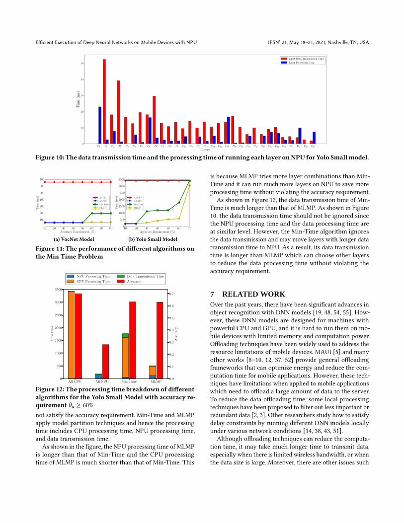
As shown in Figure 9, the data transmission time of Max-Acc is longer than that of MLMP. The reason can be betterexplained with Figure 10, which shows the data transmissiontime and the layer processing time of running each layer onNPU. For example, layer 𝐶6 needs 16ms to be processed onNPU and 19ms to move its input data from main memoryto NPU. Since the data transmission time and the NPU pro-cessing time are at similar level, the data transmission timeshould not be ignored. However, Max-Acc ignores such datatransmission time, and may move layers with longer datatransmission time to NPU. As a result, it has less optionsthan MLMP which can choose other layers to achieve higheraccuracy within the time constraint.

6.5 Comparisons of Different Algorithmson the Min-Time Problem

Figure 11 shows the performance of All-CPU, All-NPU, Max-Acc and MLMP on the Min-Time problem for the VocNetmodel and the Yolo Small model. Note that the Max-Accalgorithm is not shown here since it is designed for the Max-Accuracy problem instead of the Min-Time problem. TheAll-NPU algorithm achieves 53% and 29% accuracy on theVocNet model and the Yolo Small model, and thus it can

only be used when the accuracy requirement is below 60%in Figure 11(a) and when the accuracy requirement is below30% in Figure 11(b).As shown in the figure, the All-CPU algorithm runs all

model layers on CPU, and thus its processing time does notchange when the accuracy requirement decreases. As theaccuracy requirement decreases, model partition algorithmsuch as Min-Time and MLMP can run more model layerson NPU and hence the processing time is reduced. However,the decreasing trend is different. As shown in Figure 11(a),the processing time of MLMP is much shorter than that ofMin-Time when the accuracy requirement is between 60%to 80%. For example, when the accuracy requirement is 70%,the processing time of MLMP is 70% shorter than that ofMin-Time. This is because the accuracy drops slightly afterMin-Time moves the first three layers from CPU to NPU.However, the fourth model layer 𝑃1 (shown in Figure 8) hasthe highest high accuracy loss. After 𝑃1 is moved to NPU,the accuracy drops below 60% and thus Min-Time can onlymove three model layers from CPU to NPU. Compared toMin-Time, MLMP tries more layer combinations and canselect better layer combinations to satisfy the accuracy re-quirement. When the accuracy requirement is between 10%to 50%, Min-Time and MLMP have the same processing timesince the accuracy requirement is still satisfied when alllayers are run on NPU.As shown in Figure 11(b), the processing time of MLMP

is much shorter than that of Min-Time when the accuracyrequirement is between 30% and 70%. For example, when theaccuracy requirement is 60%, the processing time of MLMPis decreased by about 70%, compared to Min-Time. This isbecause the model layers 𝐶21 and 𝐶18 (shown in Figure 2)have long processing time and high accuracy loss and theyare the ninth and the thirteenth model layers moved fromCPU to NPU by Min-Time. After they are moved to NPU,the accuracy drops significantly. As a result, Min-Time onlymoves about ten layers from CPU to NPU. Compared to Min-Time, MLMP tries more layer combinations and then canselect better layer combinations to satisfy the accuracy re-quirement. When the accuracy requirement is between 10%to 20%, All-NPU, Min-Time and MLMP have the same pro-cessing time since the accuracy requirement is still satisfiedeven when all layers are run on NPU.Breakdownof theProcessingTime:To better understandthe performance difference among the algorithms, we breakdown the data processing time into CPU processing time,NPU processing time, and data transmission time. Figure 12shows the processing time breakdown of these algorithms forthe Yolo Small model when the accuracy requirement is 60%.As shown in the figure, All-CPU has the highest accuracybut its processing time is also the longest. All-NPU has thelowest processing time, but its accuracy is 29%, which does


C1 P1 C2 P2 C3 C4 C5 C6 P6 C7 C8 C9 C10 C11 C12 C13 C14 C15 C16 P16 C17 C18 C19 C20 C21 C22 C23 C24 F25 F26 F27

Layer

0

10

20

30

40

50

Tim

e(m

s)

Input Data Transmission Time

Layer Processing Time

Figure 10: The data transmission time and the processing time of running each layer onNPU for Yolo Smallmodel.

10 20 30 40 50 60 70 80Accuracy Requirement (%)

0

100

200

300

400

500

600

700

Tim

e(m

s) All-CPU

All-NPU

Min-Time

MLMP

(a) VocNet Model

10 20 30 40 50 60 70Accuracy Requirement (%)

0

500

1000

1500

2000

2500

3000

3500

Tim

e(m

s) All-CPU

All-NPU

Min-Time

MLMP

(b) Yolo Small Model

Figure 11: The performance of different algorithms onthe Min Time Problem

All-CPU All-NPU Min-Time MLMP0

500

1000

1500

2000

2500

3000

3500

Tim

e(m

s)

NPU Processing Time

CPU Processing Time


Accuracy

0.0

0.1

0.2

0.3

0.4

0.5

0.6

0.7

Acc

ura

cy

Figure 12: The processing time breakdown of differentalgorithms for the Yolo Small Model with accuracy re-quirement \𝑎 ≥ 60%not satisfy the accuracy requirement. Min-Time and MLMPapply model partition techniques and hence the processingtime includes CPU processing time, NPU processing time,and data transmission time.

As shown in the figure, the NPU processing time of MLMPis longer than that of Min-Time and the CPU processingtime of MLMP is much shorter than that of Min-Time. This

is because MLMP tries more layer combinations than Min-Time and it can run much more layers on NPU to save moreprocessing time without violating the accuracy requirement.

As shown in Figure 12, the data transmission time of Min-Time is much longer than that of MLMP. As shown in Figure10, the data transmission time should not be ignored sincethe NPU processing time and the data processing time areat similar level. However, the Min-Time algorithm ignoresthe data transmission and may move layers with longer datatransmission time to NPU. As a result, its data transmissiontime is longer than MLMP which can choose other layersto reduce the data processing time without violating theaccuracy requirement.

7 RELATEDWORKOver the past years, there have been significant advances inobject recognition with DNN models [19, 48, 54, 55]. How-ever, these DNN models are designed for machines withpowerful CPU and GPU, and it is hard to run them on mo-bile devices with limited memory and computation power.Offloading techniques have been widely used to address theresource limitations of mobile devices. MAUI [5] and manyother works [8–10, 12, 37, 52] provide general offloadingframeworks that can optimize energy and reduce the com-putation time for mobile applications. However, these tech-niques have limitations when applied to mobile applicationswhich need to offload a large amount of data to the server.To reduce the data offloading time, some local processingtechniques have been proposed to filter out less important orredundant data [2, 3]. Other researchers study how to satisfydelay constraints by running different DNN models locallyunder various network conditions [14, 38, 43, 51].Although offloading techniques can reduce the computa-

tion time, it may take much longer time to transmit data,especially when there is limited wireless bandwidth, or whenthe data size is large. Moreover, there are other issues such


as the lack of server support or privacy concerns, which mo-tivate the large amount of research on efficient execution ofDNNs on mobile devices. For example, DeepEye [31] reducesthe processing time and the energy consumption of runningDNNmodels on mobile devices by interleaving the executionof the convolutional layers and the fully connected layersin DNN models. Xu et al. [47] proposed a cache design toaccelerate DNN based video analytics on mobile devices. In[1, 7, 13, 15, 45], convolutional layers and fully-connectedlayers are compressed to reduce the processing time of DNNmodels. Liu et al. [28] optimize the convolutional operationsby reducing the redundant parameters in neural networks.DeepIoT [49] and FastDeepIoT [50] compress DNNmodels byoptimizing the neural network configuration. Although theefficiency can be improved through these model compressiontechniques, the accuracy also drops. The execution efficiencyof DNN models can also be improved through hardwaresupport. For example, some existing research [21, 25, 32]leverages CPU and GPU to execute the DNN models effi-ciently. Different from them, we use NPU.Instead of running the whole DNN model locally or of-

floading all computations to the cloud, some researchersleverage model partition technique to run part of the modellocally and offload the intermediate results to the server.For instance, Teerapittayanon et al. [44] distribute the DNNmodel computations across local device, edge server andcloud, and insert early exit points to reduce the processingtime. Mao et al. [30] proposes to reduce the processing timeby distributing the partitioned DNN models across mobiledevices. In Neruosurgeon [24], the DNN models are dividedinto local processing part and offloading part to optimizeenergy. In [17, 22], model partition techniques are appliedto reduce the data processing delay. However, these existingtechniques cannot be directly applied to our problem sincenone of them considers the low accuracy problem introducedby NPU.

8 CONCLUSIONSIn this paper, we developed model partition techniques toimprove the performance of running DNN models on mo-bile devices with NPU. Based on the delay and accuracyrequirements of the applications, we studied two problems:Max-Accuracy where the goal is to maximize the accuracy un-der some time constraints, andMin-Time where the goal is tominimize the processing time while ensuring that accuracyis above a certain threshold. We have identified some specialcharacteristics of running DNN models on mobile deviceswith NPU.We formalized theMax-Accuracy problem and theMin-Time problem, and proposed heuristic based solutionsto solve them based on the identified special characteristics.More specifically, we proposed model partition techniques to

determine which layers to run on CPU and which layers torun on NPU to satisfy the application requirements on delayand accuracy. We identified some limitations of the heuristicbased algorithms, and proposed a Machine Learning basedModel Partition (MLMP) algorithm to further improve theperformance. MLMP leverages machine learning techniqueto estimate the accuracy loss of running the DNN modelwith a layer combination. Since the SDK for NPU does notinclude tools to measure the layer processing time on NPU,and the data transmission time between NPU and memory,we proposed techniques to better estimate them and thenefficiently search for the best layer combinations to solve theMax-Accuracy problem and the Min-Time problem. We alsoaddressed many implementation issues to support modelpartition techniques on mobile devices with NPU. Exten-sive evaluation results show that MLMP can significantlyimprove the accuracy or reduce the processing time basedon the application requirements.

ACKNOWLEDGMENTSThis work was supported in part by the National ScienceFoundation (NSF) under grant CNS-1815465.

REFERENCES[1] S. Bhattacharya and N. Lane. 2016. Sparsification and Separation of

Deep Learning Layers for Constrained Resource Inference on Wear-ables. ACM Sensys (2016).

[2] Y. Chen, L. Ravindranath, S. Deng, P. Bahl, and H. Balakrishnan. 2015.Glimpse: Continuous, Real-Time Object Recognition on Mobile De-vices. ACM Sensys (2015).

[3] K. Chen, T. Li, H. Kim, D. Culler, and R. Katz. 2018. MARVEL: EnablingMobile Augmented Reality with Low Energy and Low Latency. ACMSensys (2018).

[4] J. Chorowski, D. Bahdanau, D. Serdyuk, K. Cho, and Y. Bengio. 2015.Attention-Based Models for Speech Recognition. NIPS (2015).

[5] E. Cuervo, A. Balasubramanian, D. Cho, A. Wolman, S. Saroiu, R. Chan-dra, and P. Bahl. 2010. MAUI: Making Smartphones Last Longer withCode Offload. ACM Int’l Conf. on Mobile Systems Applications andServices (MobiSys) (2010).

[6] M. Everingham, S. Eslami, L. Van Gool, C. Williams, J. Winn, andA. Zisserman. 2015. The Pascal Visual Object Classes Challenge: ARetrospective. Springer International Journal of Computer Vision (IJCV)(2015).

[7] B. Fang, X. Zeng, and M. Zhang. 2018. Nestdnn: Resource-AwareMulti-Tenant On-Device Deep Learning for Continuous Mobile Vision.ACM Mobicom (2018).

[8] Y. Geng and G. Cao. 2018. Peer-Assisted Computation Offloading inWireless Networks. IEEE Transactions on Wireless Communications 17,7 (2018), 4565–4578.

[9] Y. Geng, W. Hu, Y. Yang, W. Gao, and G. Cao. 2015. Energy-EfficientComputation Offloading in Cellular Networks. IEEE ICNP (2015).

[10] Y. Geng, Y. Yang, and G. Cao. 2018. Energy-Efficient ComputationOffloading for Multicore-based Mobile Devices. IEEE Infocom (2018).

[11] Google. [n.d.]. Android NDK. https://developer.android.com/ndk.[12] M. Gordon, D. Jamshidi, S. Mahlke, Z. Mao, and X. Chen. 2012. COMET:

Code Offload by Migrating Execution Transparently. ACM USENIX


Symposium on Operating Systems Design and Implementation (OSDI)(2012).

[13] S. Han, H. Mao, and W. Dally. 2016. Deep Compression: CompressingDeep Neural Networks with Pruning, Trained Quantization and Huff-man Coding. IEEE International Conference on Learning Representations(ICLR) (2016).

[14] S. Han, H. Shen, M. Philipose, S. Agarwal, A. Wolman, and A. Kr-ishnamurthy. 2016. MCDNN: An Approximation-Based ExecutionFramework for Deep Stream Processing Under Resource Constraints.ACM Int’l Conf. on Mobile Systems Applications and Services (MobiSys)(2016).

[15] S. Han, J. Pool, J. Tran, and W. Dally. 2015. Learning both Weights andConnections for Efficient Neural Network. NIPS (2015).

[16] K. He, X. Zhang, S. Ren, and J. Sun. 2015. Delving Deep into Rectifiers:Surpassing Human-Level Performance on ImageNet Classification.IEEE ICCV (2015).

[17] C. Hu, W. Bao, D. Wang and F. Liu. 2019. Dynamic Adaptive DNNSurgery for Inference Acceleration on the Edge. IEEE Infocom (2019).

[18] G. Huang, R. Manu, B. Tamara, and L. Erik. 2007. Labeled Faces in theWild: A Database for Studying Face Recognition in Unconstrained Envi-ronments. Technical Report. University of Massachusetts, Amherst.

[19] G. Huang, Z. Liu, L. Van Der Maaten, and K.Weinberger. 2017. DenselyConnected Convolutional Networks. IEEE CVPR (2017).

[20] HUAWEI. 2019. Kirin 990. https://consumer.huawei.com/en/campaign/kirin-990-series/.

[21] L. Huynh, Y. Lee, and R. Balan. 2017. DeepMon: Mobile GPU-basedDeep Learning Framework for Continuous Vision Applications. ACMInt’l Conf. onMobile Systems Applications and Services (MobiSys) (2017).

[22] Y. Ikeda, Y. Yanagisawa, Y. Kishino, S. Mizutani, Y. Shirai, T. Suyama,K. Matsumura, and H. Noma. 2018. Reduction of Communication Costfor Edge-Heavy Sensor using Divided CNN. IEEE International Confer-ence on Embedded and Real-Time Computing Systems and Applications(2018).

[23] Y. Jia, E. Shelhamer, J. Donahue, S. Karayev, J. Long, R. Girshick, S.Guadarrama, and T. Darrell. 2014. Caffe: Convolutional Architecturefor Fast Feature Embedding. ACM International Conference on Multi-media (2014).

[24] Y. Kang, J. Hauswald, C. Gao, A. Rovinski, T. Mudge, J. Mars, and L.Tang. 2017. Neurosurgeon: Collaborative Intelligence Between theCloud and Mobile Edge. ACM SIGARCH (2017).

[25] N. Lane, S. Bhattacharya, P. Georgiev, C. Forlivesi, L. Jiao, L. Qendro,and F. Kawsar. 2016. DeepX: A Software Accelerator for Low-PowerDeep Learning Inference on Mobile Devices. IEEE International Con-ference on Information Processing in Sensor Networks (IPSN) (2016).

[26] S. Lapuschkin, A. Binder, G. Montavon, K.-R. Müller, and W. Samek.2016. Analyzing classifiers: Fisher vectors and deep neural networks.IEEE CVPR (2016).

[27] T. Lin, M. Maire, S. Belongie, J. Hays, P. Perona, D. Ramanan, P. Dollárand C. Zitnick. 2014. Microsoft COCO: Common Objects in Context.European Conference on Computer Vision (ECCV) (2014).

[28] B. Liu, M. Wang, H. Foroosh, M. Tappen and M. Pensky. 2015. SparseConvolutional Neural Networks. IEEE CVPR (2015).

[29] X. Liu, P. He, W. Chen, and J. Gao. 2019. Multi-Task Deep NeuralNetworks for Natural Language Understanding. Annual Meeting of theAssociation for Computational Linguistics (2019).

[30] J. Mao, Z. Yang, W. Wen, C. Wu, L. Song, K. Nixon, X. Chen, H. Li, andY. Chen. 2017. Mednn: A Distributed Mobile System with EnhancedPartition and Deployment for Large-Scale DNNs. IEEE InternationalConference on Computer-Aided Design (2017).

[31] A. Mathur, N. Lane, S. Bhattacharya, A. Boran, C. Forlivesi, and F.Kawsar. 2017. DeepEye: Resource Efficient Local Execution of MultipleDeep Vision Models using Wearable Commodity Hardware. ACM Int’l

Conf. on Mobile Systems Applications and Services (MobiSys) (2017).[32] L. Oskouei, S. Salar, H. Golestani, M. Hashemi and S. Ghiasi. 2016.

CNNdroid: GPU-Accelerated Execution of Trained Deep Convolu-tional Neural Networks on Android. ACM International Conference onMultimedia (2016).

[33] J. Park, Y. Boo, I. Choi, S. Shin, andW. Sung. 2018. Fully Neural NetworkBased Speech Recognition on Mobile and Embedded Devices. NIPS(2018).

[34] O. M. Parkhi, A. Vedaldi, A. Zisserman. 2015. Deep Face Recognition.British Machine Vision Conference (2015).

[35] F. Pedregosa, G. Varoquaux, A. Gramfort, V. Michel, B. Thirion, O.Grisel, M. Blondel, P. Prettenhofer, R. Weiss, V. Dubourg, J. Vanderplas,A. Passos, D. Cournapeau, M. Brucher, M. Perrot, and E. Duchesnay.2011. Scikit-learn: Machine Learning in Python. Journal of MachineLearning Research (2011).

[36] Qualcomm. [n.d.]. Snapdragon 855.https://www.qualcomm.com/products/snapdragon-855-mobile-platform.

[37] M. Ra, A. Sheth, L. Mummert, P. Pillai, D. Wetherall, and R. Govindan.2011. Odessa: Enabling Interactive Perception Applications on MobileDevices. ACM Int’l Conf. on Mobile Systems Applications and Services(MobiSys) (2011).

[38] X. Ran, H. Chen, X. Zhu, Z. Liu, and J. Chen. 2018. DeepDecision: AMobile Deep Learning Framework for Edge Video Analytics. IEEEInfocom (2018).

[39] J. Redmon, S. Divvala, R. Girshick, and A. Farhadi. 2016. You OnlyLook Once: Unified, Real-Time Object Detection. IEEE CVPR (2016).

[40] Samsung. [n.d.]. Samsung Electronics to Strengthen itsNeural Processing Capabilities for Future AI Applications.https://news.samsung.com/global/samsung-electronics-to-strengthen-its-neural-processing-capabilities-for-future-ai-applications.

[41] T. Sattler, M. Havlena, K. Schindler, and M. Pollefeys. 2016. Large-ScaleLocation Recognition and the Geometric Burstiness Problem. IEEECVPR (2016).

[42] H. Taira, M. Okutomi, T. Sattler, M. Cimpoi, M. Pollefeys, J. Sivic, T.Pajdla and A. Torii. 2018. InLoc: Indoor Visual Localization with DenseMatching and View Synthesis. IEEE ICCV (2018).

[43] T. Tan and G. Cao. 2020. FastVA: Deep Learning Video AnalyticsThrough Edge Processing and NPU in Mobile. IEEE INFOCOM (2020).

[44] S. Teerapittayanon, B. McDanel and H. Kung. 2017. Distributed DeepNeural Networks Over the Cloud, the Edge and End Devices. IEEEInternational Conference on Distributed Computing Systems (ICDCS)(2017).

[45] W. Wen, C. Wu, Y. Wang, Y. Chen, and H. Li. 2016. Learning StructuredSparsity in Deep Neural Networks. NIPS (2016).

[46] W. Xiong, J. Droppo, X. Huang, F. Seide, M. Seltzer, A. Stolcke, D. Yu,and G. Zweig. 2017. Toward Human Parity in Conversational SpeechRecognition. IEEE/ACM Transactions on Audio, Speech and LanguageProcessing (TASLP) (2017).

[47] M. Xu, and M. Zhu, and Y. Liu, and F. Lin, and X. Liu. 2018. DeepCache:Principled Cache for Mobile Deep Vision. ACM Mobicom (2018).

[48] S. Yang and D. Ramanan. 2015. Multi-scale recognition with DAG-CNNs. IEEE ICCV (2015).

[49] S. Yao, Y. Zhao, A. Zhang, L. Su, and T. Abdelzaher. 2017. DeepIoT:Compressing Deep Neural Network Structures for Sensing Systemswith a Compressor-Critic Framework. ACM Sensys (2017).

[50] S. Yao, Y. Zhao, H. Shao, S. Liu, D. Liu, L. Su, Lu and T. Abdelzaher.2018. FastDeepIoT: Towards Understanding and Optimizing NeuralNetwork Execution Time on Mobile and Embedded Devices. ACMSensys (2018).


[51] S. Yi, Z. Hao, Q. Zhang, Q. Zhang, W. Shi, and Q. Li. 2017.Lavea: Latency-Aware Video Analytics on Edge Computing Platform.ACM/IEEE Symposium on Edge Computing (2017).

[52] I. Zhang, A. Szekeres, A. Van, I. Ackerman, S. Gribble, A. Krishna-murthy, and H. Levy. 2014. Customizable and Extensible Deploymentfor Mobile/Cloud Applications. ACM USENIX Symposium on OperatingSystems Design and Implementation (OSDI) (2014).

[53] H. Zhang, C. Song, A. Wang, C. Xu, D. Li, and W. Xu. 2019. PDVocal:Towards Privacy-preserving Parkinson’s Disease Detection using Non-speech Body Sounds. ACM Mobicom (2019).

[54] Y. Zhang, K. Lee, and H. Lee. 2016. Augmenting Supervised NeuralNetworks with Unsupervised Objectives for Large-scale Image Clas-sification. IEEE International Conference on Machine Learning (ICML)(2016).

[55] J. Zhang, Z. Tang, M. Li, D. Fang, P. Nurmi, and Z. Wang. 2018.CrossSense: Towards Cross-Site and Large-Scale WiFi Sensing. ACMMobicom (2018).

efficient execution of deep neural networks on mobile

Documents