ORIGINAL ARTICLE

Efficient Spiking Neural Network Model of Pattern MotionSelectivity in Visual Cortex

Michael Beyeler & Micah Richert & Nikil D. Dutt &Jeffrey L. Krichmar

Abstract Simulating large-scale models of biological motionperception is challenging, due to the required memory to storethe network structure and the computational power needed toquickly solve the neuronal dynamics. A low-cost yet high-performance approach to simulating large-scale neural net-work models in real-time is to leverage the parallel processingcapability of graphics processing units (GPUs). Based on thisapproach, we present a two-stage model of visual areaMT thatwe believe to be the first large-scale spiking network todemonstrate pattern direction selectivity. In this model,component-direction-selective (CDS) cells in MT linearlycombine inputs from V1 cells that have spatiotemporal recep-tive fields according to the motion energymodel of Simoncelliand Heeger. Pattern-direction-selective (PDS) cells in MT areconstructed by pooling over MT CDS cells with a wide rangeof preferred directions. Responses of our model neurons arecomparable to electrophysiological results for grating andplaid stimuli as well as speed tuning. The behavioral responseof the network in a motion discrimination task is in agreementwith psychophysical data. Moreover, our implementation out-performs a previous implementation of the motion energymodel by orders of magnitude in terms of computationalspeed and memory usage. The full network, which comprises153,216 neurons and approximately 40 million synapses,processes 20 frames per second of a 40×40 input video inreal-time using a single off-the-shelf GPU. To promote the useof this algorithm among neuroscientists and computer vision

researchers, the source code for the simulator, the network,and analysis scripts are publicly available.

Keywords Pattern motion selectivity . Spiking neuralnetwork .MT . GPU . Real-time . CARLsim

Introduction

Visual motion perception is a challenging problem that iscritical for navigating through the environment and trackingobjects. Several software packages are available to the publicthat deal with the neurobiologically plausible modeling ofmotion perception in the mammalian brain, such asspatiotemporal-energy models like the motion energy modelof Simoncelli and Heeger (1998), or gradient-based modelslike ViSTARS (Browning et al. 2009a, b). However, in orderfor these frameworks to become practical in, for example,neuromorphic or robotics applications, they must be capableof running large-scale networks in real-time. Moreover, totake advantage of state-of-the-art neuromorphic hardware,the elements of the algorithms need to be spiking neurons(Indiveri et al. 2006; Merolla et al. 2007; Vogelstein et al.2007; Khan et al. 2008; Srinivasa and Cruz-Albrecht 2012).Developing such a simulation environment is challenging,due to the required memory to store the network structureand the computational power needed to quickly solve theequations describing the neuronal dynamics. A low-cost yethigh-performance approach to simulating large-scale spikingneural networks (SNNs) in real-time is to leverage the parallelprocessing capability of graphics processing units (GPUs)(Nageswaran et al. 2009; Fidjeland and Shanahan 2010;Yudanov et al. 2010; Richert et al. 2011).

Based on this approach, we present a two-stage model ofvisual area MT that we believe to be the first large-scalespiking network to demonstrate pattern direction selectivity.The model combines and extends two previous incarnations of

M. Beyeler (*) :N. D. Dutt : J. L. KrichmarDepartment of Computer Science, University of California, Irvine,Irvine, CA 92697, USAe-mail: mbeyeler@uci.edu

M. Richert : J. L. KrichmarDepartment of Cognitive Sciences, University of California Irvine,Irvine, CA, USA

M. RichertBrain Corporation, San Diego, CA, USA

Neuroinform (2014) 12:435–454DOI 10.1007/s12021-014-9220-y

Published online: 5 February 2014# Springer Science+Business Media New York 2014

the motion energy model (Simoncelli and Heeger 1998; Rustet al. 2006). Broadly speaking, our model integrates the V1stage of Simoncelli and Heeger (1998) with the MT stage ofRust et al. (2006) in the spiking domain. More precisely, ourmodel uses a bank of spatiotemporal filters (Adelson andBergen 1985; Simoncelli and Heeger 1998) to model thereceptive fields of directionally selective neurons in V1, whichthen project to component-direction-selective (CDS) cells inarea MT. However, the local motion estimates coded by thespike patterns of these neurons often vary drastically from theglobal pattern motion of a visual stimulus, because the localmotion of a contour is intrinsically ambiguous (“aperture prob-lem”). Therefore, in order to construct pattern-direction-selective (PDS) cells in MT that signal the global patternmotion, we implemented three design principles introducedby Rust et al. (2006): 1) spatial pooling over V1 or MT CDScells with a wide range of preferred directions, 2) strongmotion opponent suppression, and 3) a tuned normalizationthat may reflect center-surround interactions in MT. Whereasthe implementation by Rust et al. (2006) was restricted toinputs that are mixtures of sinusoidal gratings of a fixed spatialand temporal frequency, our model can operate on any spatio-temporal image intensity.

The motion energy model of Simoncelli and Heeger (1998),henceforth referred to as the S&H model, is conceptuallyequivalent to an elaborated Reichardt detector at the end ofthe V1 stage (van Santen and Sperling 1985), and is a specificimplementation of the intersection-of-constraints (IOC) princi-ple at the end of the MT PDS stage (Bradley and Goyal 2008).The IOC principle in turn is one possible solution to theaperture problem; that is, a velocity-space construction thatfinds the global pattern motion as the point in velocity-spacewhere the constraint lines of all local velocity samples inter-sect. Adelson and Movshon (1982) differentiated among threemethods to estimate the global pattern motion; 1) IOC princi-ple, 2) vector average (VA), and 3) blob or feature tracking,which may be equally valid approaches to solving the apertureproblem (for a recent review on the topic see Bradley andGoyal (2008)). Although the S&H model is not complete, inthe sense that it does not specify the exact pattern or objectvelocity, the model in particular and the IOC principle ingeneral are consistent with various experimental data.

In the present paper, we introduce a large-scale spikingneuron model of cortical areas critical for motion processing,which is efficient enough to run in real-time on availableprocessors. We show that the responses of neurons in thenetwork are comparable to electrophysiological results forgrating and plaid stimuli, as well as speed tuning. The behav-ioral response of the network in a two-alternative forced choice(2AFC) motion discrimination task (that is, a random dotmotion coherence task) is in agreement with psychophysicaldata. Moreover, our implementation outperforms a previousrate-based C/Matlab implementation of the S&H model by up

to a factor of 12 in terms of computational speed and by ordersof magnitude in terms of memory usage. The full network,which comprises 153,216 neurons and approximately 40 mil-lion synapses, processes 20 frames per second of a 40×40input video in real-time using a single off-the-shelf GPU.

The network was constructed using an open-source SNNsimulator (Richert et al. 2011) that provides a PyNN-likeprogramming interface; its neuron model, synapse model, andaddress-event representation (AER) are compatible with recentneuromorphic hardware (Srinivasa and Cruz-Albrecht 2012).To promote the use of this algorithm among the neuroscientistand computer vision research communities, the source code forthe simulator, the network, and analysis scripts are publiclyavailable at http://www.socsci.uci.edu/~jkrichma/CARLsim/.

Methods

The Simulator

The present model was developed on a simulator that waspreviously published in Nageswaran et al. (2009) and Richertet al. (2011). The first study demonstrated real-time perfor-mance for a simulation of 100,000 neurons on a singleNVIDIA C1060 GPU. The latter added a wide range of func-tionalities, such as equations for synaptic conductances, spike-timing-dependent plasticity (STDP), and short-term plasticity(STP). The present release builds on this mainly by: 1) provid-ing the complete source code for a detailed large-scale modelof visual motion processing in V1 and MT, 2) improving theoriginal model to demonstrate PDS responses and speedtuning, and 3) introducing source code-level optimizations thatimprove GPU memory management and ensure code stability.Whereas the optimizations should be applicable to a widerange of GPU architectures, they are not directly relevant tothis paper and will thus not be discussed (for more informationplease refer to the release notes).

The main code to run the experiments described in thispaper can be found in the file “examples/v1MTLIP/main_v1MTLIP.cpp”, which is part of the CARLsim 2.1software package. The “examples” directory also containsa number of other experiments that were part of a previouscode release—for more information refer to Richert et al.(2011). Matlab scripts to analyze the network output andcreate the figures can be found in the directory “scripts/v1MTLIP/”. Please note that Matlab is not necessary to usethe simulator, as the scripts are provided mainly for analysispurposes.

Setting up a Simulation

Step-by-step instructions on how to set up, interact with, andrun a simulation can be found in the tutorial on our website

436 Neuroinform (2014) 12:435–454

and in our previous code release (Richert et al. 2011). For thereader’s convenience, we include here a representative exam-ple to illustrate the ease of setting up and running a simulation.Listing 1 randomly connects ten Poisson spike generators

(gIn) firing at 50 Hz mean rate to a population of 100excitatory Izhikevich neurons (gEx), records and stores thespike times in a binary file “spkEx.dat”, and runs thenetwork for a second of simulation time:

In this example, connectivity (achieved throughCpuSNN:connect(…)) is random with an initial weightof 1.0, a maximum weight of 1.0, a 10 % (0.10) connectionprobability, a synaptic delay uniformly distributed between1 ms and 20 ms, and static synapses (SYN_FIXED). Note thatany type of connectivity profile is possible by using a callbackmechanism. For a description of the Izhikevich neuron modelplease refer to section “Neuron Model”.

CPU vs. GPU Simulation Mode

A major advantage of our simulator is the possibility torun a simulation either on standard x86 central process-

ing units (CPUs) or off-the-shelf NVIDIA GPUs, simplyby passing a constant with value CPU_MODE orGPU_MODE as an additional function argument toCpuSNN::runNetwork(…). A new feature is the op-tion to pass a “device index” to the same method, whichcan be used in multi-GPU systems to specify on whichCUDA device to establish a context. For example,Listing 2 would run a built network for 1 second onthe second GPU (if such a device exists):

The two simulation modes allow the user to exploit theadvantages of both architectures. Whereas the CPU is more

efficient for relatively small networks, the GPU is most ad-vantageous for network sizes of 1,000 neurons and up

#include "snn.h" CpuSNN sim("My network");

// set up network int gIn=sim.createSpikeGeneratorGroup("input", 10, EXCITATORY_NEURON); int gEx=sim.createGroup("excitatory", 100, EXCITATORY_NEURON); sim.setNeuronParameters(gEx, 0.02f, 0.2f, -65.0f, 8.0f); // RS neurons sim.connect(gIn, gEx, "random", 1.0, 1.0, 0.10f, 1, 20, SYN_FIXED);

// write spike times to file sim.setSpikeMonitor(gEx, "spkEx.dat");

// set spike rates and run network PoissonRate inSpikes(100); for (int i=0; i<100; i++) inSpikes.rates[i] = 50.0f; // 50 Hz sim.setSpikeRate(gIn, &inSpikes); sim.runNetwork(1,0); // run for 1 sec and 0 msec

Listing 1

CpuSNN sim(“My network”);... // build network int run_sec = 1; int run_msec = 0; // run for 1 s and 0 ms bool onGPU = true; // run on GPU int ithGPU = 1; // run on 2nd device (0-indexed) sim.runNetwork(run_sec, run_msec, onGPU?GPU_MODE:CPU_MODE, ithGPU);

Listing 2

Neuroinform (2014) 12:435–454 437

(Nageswaran et al. 2009; Richert et al. 2011). It has beendemonstrated that a GPU implementation (on NVIDIAGTX-280 with 1 GB of memory) for a simulation of100,000 neurons and 50 million synaptic connections canrun up to 26 times faster than a CPU version (Core2 4600@ 2.13 GHz with 4 GB of memory) of the same network(Nageswaran et al. 2009). On the other hand, the CPU modeallows for execution of extremely large networks that wouldnot fit within the GPU’s memory.

It is worth noting that a simulation can be run in CPUmodeeven if the code is compiled in the presence of CUDA sourcefiles. An example of this hybrid mode is the network ex-plained in the present work, which contains a V1 stage purelywritten in CUDA. In this case the network would be allocatedon the CPU’s memory, but the generation of motion energyresponses would be delegated to the GPU.

Neuron Model

The simulator currently supports four parameter Izhikevichpoint-neurons (Izhikevich 2003). Other neuron models willfollow in future releases. The Izhikevich model aims to reduceHodgkin-Huxley-type neuronal models to a two-dimensionalsystem of ordinary differential equations,

dv tð Þdt

¼ 0:04v2 tð Þ þ 5v tð Þ þ 140−u tð Þ þ isyn tð Þ ð1Þ

du tð Þdt

¼ a b v tð Þ−u tð Þð Þ: ð2Þ

Here (1) describes the membrane potential v for a givenexternal current isyn, whereas (2) describes a recovery vari-able u; the parameter a is the rate constant of the recoveryvariable, and the parameter b describes the sensitivity of therecovery variable to the subthreshold fluctuations of themembrane potential. All parameters in (1) and (2) are di-mensionless; however, the right-hand side of (1) is in a formsuch that the membrane potential v has mV scale and thetime t has ms scale (Izhikevich 2003). The Izhikevich modelis well-suited for large-scale simulations, because it is com-putationally inexpensive yet capable of spiking, bursting,and being either an integrator or a resonator (Izhikevich2004, 2007).

In contrast to other simple models such as the leakyintegrate-and-fire (LIF) neuron, the Izhikevich neuron is ableto generate the upstroke of the spike itself. Thus the voltagereset occurs not at the threshold, but at the peak (vcutoff=+30),of the spike. The action potential downstroke is modeled usingan instantaneous reset of the membrane potential whenever v

reaches the spike cutoff, plus a stepping of the recoveryvariable:

v v > 30ð Þ ¼ c and u v > 30ð Þ ¼ u−d: ð3Þ

The inclusion of u in the model allows for the simulation oftypical spike patterns observed in biological neurons. The fourparameters a, b, c, and d can be set to simulate different typesof neurons. Unless otherwise specified, excitatory neurons inall our simulations were modeled as regular spiking (RS)neurons (class 1 excitable, a=0.02,b=0.2, c=−65, d=8),and all inhibitory neurons were modeled as fast spiking (FS)neurons (class 2 excitable, a=0.1, b=0.2, c=−65, d=2)(Izhikevich 2003, 2004).

Synapse Model

A simulation can be run with either a current-based or aconductance-based neuron model (sometimes referred to asCUBA and COBA, respectively). All experiments in thepresent study were run in COBA mode.

In a conductance-based model, each ionic current thatcontributes to the total current isyn (see (1)) is associated witha conductance. The simulator supports four of the most prom-inent synaptic conductances found in the cortex: AMPA (fastdecay), NMDA (slow decay and voltage-dependent), GABAa(fast decay), and GABAb (slow decay), which are modeled asdynamic synaptic channels with zero rise time and exponen-tial decay according to

dgr tð Þdt

¼ −1

τ rgr tð Þ þ w

Xi

δ t−tið Þ; ð4Þ

where δ is the Dirac delta, the sum is over all presynaptic spikesarriving at times ti,w is the weight of that synapse, τr is its decaytime constant, and the subscript r denotes the receptor type; thatis, AMPA, NMDA, GABAa, or GABAb. Unless otherwisespecified, a spike arriving at a synapse that is post-synapticallyconnected to an excitatory (inhibitory) neuron increases bothgAMPA and gNMDA (gGABAa

and gGABAbÞ: In our simulations

we set the time constants to τAMPA ¼ 5 ms; τNMDA ¼ 150 ms;τGABAa ¼ 6 ms; and τGABAb ¼ 150 ms (Dayan and Abbott2001; Izhikevich et al. 2004). The rise time of these conduc-tances was modeled as instantaneous, which is a reasonableassumption in the case of AMPA, NMDA, and GABAa

(Dayan and Abbott 2001), but a simplification in the case ofGABAb, which has a rise time on the order of 10 ms (Koch1999).

Then the total synaptic current isyn in (1) for each neuron isgiven by:

438 Neuroinform (2014) 12:435–454

isyn ¼ −gAMPA v−0ð Þ

−gNMDA

vþ8060

� �21þ vþ80

60

� �2 v−0ð Þ−gGABAa vþ 70ð Þ−gGABAb

vþ 90ð Þ

; ð5Þ

where v is the membrane potential of the neuron, and thesubscript indicates the receptor type. This equation is equiva-lent to the one described in Izhikevich et al. (2004).

The Network

The network architecture is shown in Fig. 1. Grayscale videosare fed frame-by-frame through a model of the primary visualcortex (V1), the middle temporal area (MT), and the lateralintraparietal cortex (LIP). Bold black arrows indicate synapticprojections. Note that inhibitory populations and projectionsare not shown for the sake of clarity. Numbers in parenthesesnext to an element are the equations that describe the corre-sponding neuronal response or synaptic projections, as will beexplained in the subsections below.

The V1 model consisted of a bank of spatiotemporal filters(rate-based) according to the S&H model (Simoncelli andHeeger 1998), which will be described in detail in section“Spatiotemporal-EnergyModel of V1”. At each point in time,a 32×32 input video frame was processed by V1 cells at threedifferent spatiotemporal resolutions (labeled “3 scales” inFig. 1). Simulated V1 simple cells computed an inner productof the image contrast with one of 28 space-time orientedreceptive fields (third derivatives of a Gaussian), which wasthen half-wave rectified, squared, and normalized within alarge Gaussian envelope. V1 complex cell responses werecomputed as a weighted sum of simple cell afferents thathad the same space-time orientation, but were distributed overa local spatial region. We interpreted these filter responses asmean firing rates of Poisson spike trains (labeled “Hz” in thefigure) as explained in section “Spatiotemporal-EnergyModelof V1”, which were first scaled to match the contrast sensitiv-ity function of V1 simple cells, and then used to driveIzhikevich spiking neurons representing cells in area MT.

Area MT consisted of two distinct populations of spikingneurons (explained in section “Two-Stage Spiking Model ofMT”), the first one being selective to all local componentmotions of a stimulus (CDS cells), and the other oneresponding to the global pattern motion (PDS cells). MTCDS cells responded to three different speeds (1.5 pixels/frame, 0.125 pixels/frame, and 9 pixels/frame) illustrated asthree distinct populations in the MT CDS layer of Fig. 1.Divisive normalization between these populations enabledthe generation of speed tuning curves that are in agreementwith neurophysiological experiments (Rodman and Albright

1987). The three MT CDS populations consisted of eightsubpopulations, each of which was not only selective to aparticular speed but also to one of eight directions of motion,in 45° increments. PDS cells were constructed by 1) poolingover MT CDS cells with a wide range of preferred directions,2) using strong motion opponent suppression, and 3)employing a tuned normalization that may reflect center-surround interactions inMT (Rust et al. 2006). PDS cells wereselective to the same speed as their CDS afferents. For thepurpose of this paper we only implemented PDS cells selec-tive to a speed of 1.5 pixels/frame (see MT PDS layer inFig. 1) to be used in a motion discrimination task. However,it is straightforward to implement PDS cells that are selectiveto another speed.

A layer of decision neurons (see section “Spiking Layer ofLIP Decision Neurons”) was responsible for integrating overtime the direction-specific sensory information that is encodedby the responses ofMTPDS cells. Analogous to theMT layer,the decision layer consisted of eight subpopulations, each ofwhich received projections from a subpopulation of MT PDScells selective to one of eight directions of motion. Thisinformation was then used to make a perceptual decisionabout the presented visual stimulus, such as determining theglobal drift direction of a field of random moving dots in amotion discrimination task (presented in section “RandomDot Kinematogram”). Figure 1 exemplifies this situation byshowing a snapshot of the network’s response to a random dotkinematogram (RDK) where dots drift to the right at a speedof 1.5 pixels/frame. The subpopulation of decision neuronsthat is coding for rightward motion is activated the strongest.The temporal integration of sensory information might beperformed in one of several parietal and frontal cortical re-gions in the macaque, such as LIP, where neurons have beenfound whose firing rate are predictive of the behavioral reac-tion time (RT) in a RDK task (Shadlen and Newsome 2001;Roitman and Shadlen 2002).

The following subsections will explain the model in detail.

Spatiotemporal-Energy Model of V1

The first (V1) stage of the S&H model was implemented andtested in a Compute Unified Device Architecture (CUDA)environment (Richert et al. 2011). This part of the model isequivalent to Eqs. 1–4 in Simoncelli and Heeger (1998) andtheir subsequently released C/Matlab code, which can beobtained from: http://www.cns.nyu.edu/~lcv/MTmodel/.Unless otherwise stated, we used the same scaling factorsand parameter values as in the S&H model.

A visual stimulus is represented as a light intensity distribu-tion I(x,y,t), that is, a function of two spatial dimensions (x,y)and time t. The stimulus was processed at three differentspatiotemporal resolutions (or scales), r (labeled “3 scales” inFig. 1). The first scale, r=0, was equivalent to processing at the

Neuroinform (2014) 12:435–454 439

original image (and time) resolution. The other two scales wereachieved by successively blurring the image with a Gaussiankernel. The three stimuli Ir(x,y,t) can thus be expressed as:

I0 x; y; tð Þ ¼ I x; y; tð ÞI1 x; y; tð Þ ¼ exp

− x2 þ y2 þ t2ð Þ2

� �*I0 x; y; tð Þ

I2 x; y; tð Þ ¼ exp− x2 þ y2 þ t2ð Þ

2

� �*I1 x; y; tð Þ;

ð6Þ

where * denotes convolution. In order to circumvent the non-causality of these convolutions (the response depends both onpast and future stimulus intensities), a time delay of fourframes was introduced (see (Simoncelli and Heeger 1998)).

V1 Simple Cells A large body of research has found thatneurons located in V1 that project to MT are directionallyselective and may be regarded as local motion energy filters(Adelson and Bergen 1985; DeAngelis et al. 1993; Movshonand Newsome 1996). In our network, V1 simple cells aremodeled as linear space-time-oriented filters whose receptive

Ret

ina

InputGrayscale

spik

ing

LIP Output

LIP decision

50 Hz

0 Hz

MT

MT PDS

MT CDS

50 Hz0 Hz

50 Hz0 Hz

V1

V1 simple

V1 complex

rate

-bas

ed

50 Hz

0 Hz

100 Hz

0 Hz

...

... ... ...

3 scales

(eqns. 1 - 5)

(eqns. 1 - 5)

(eqns. 1 - 5)

(eqn. 11)

(eqn. 10)

(eqn. 6)

(eqn. 12)

(eqn. 13)

Fig. 1 Network architecture. 32×32 grayscale images are fed throughmodel V1, MT, and LIP (as explained in sections “Spatiotemporal-Ener-gy Model of V1 – Spiking Layer of LIP Decision Neurons”). Shown is asnapshot in time of the network’s response to an example RDK stimulusin which 50 % of the dots drift to the right. Black bold arrows denotesynaptic projections. Inhibitory projections and populations are not

shown. Numbers in parentheses next to an element are the equations thatdescribe the corresponding neuronal response or synaptic projections (seetext). V1 filter responses were mapped onto mean firing rates by repro-ducing the contrast sensitivity function reported for V1 cells projecting toMT, as explained in section “Spatiotemporal-Energy Model of V1”

440 Neuroinform (2014) 12:435–454

fields are third derivatives of a Gaussian (Simoncelli andHeeger 1998). These filters are very similar to a Gabor filter,but more computationally convenient as they allow for sepa-rable convolution computations.

The full set of V1 linear receptive fields consisted of 28space-time orientations that are evenly distributed on thesurface of a sphere in the spatiotemporal frequency domain.The k th space-time-oriented filter in the V1 population can be

described by a unit vector buk ¼ buk;x;buk;y;buk;t� �0that is par-

allel to the filter orientation, where k=1,2,…,28 and ' denotesvector transposition. For more information please refer toSimoncelli and Heeger (1998). An example of a spatiotempo-ral receptive field is illustrated in Fig. 2, where the coloredovals correspond to the orientation of the positive (green) andnegative (red) lobes of the spatiotemporal filter. If a driftingdot traces out a path (dashed line) in space (x, for now ignoringy) and time (t) that is oriented in the same way as the lobes,then the filter could be activated by this motion (Fig. 2a). A

dot moving in the orthogonal direction would not elicit a filterresponse because its path intersects both positive and negativelobes of the filter (as depicted in Fig. 2b).

First, input images were filtered with a 3D Gaussian cor-responding to the receptive field size of a V1 simple cell:

f r x; y; tð Þ ¼ exp− x2 þ y2 þ t2ð Þ

2σ2v1simple

!� I r x; y; tð Þ ð7Þ

where * is the convolution operator, r denotes the scale, andσv1simple=1.25 pixels.

Then the underlying linear response of a simple cell atspatial location (x,y) and scale r with space-time orientationk is equivalent to the third-order derivative in the direction of

u ̂k ; that is,

Lkr x; y; tð Þ ¼ αv1lin

XT¼0

3 X3−TY¼0

3!

X !Y !T !buk;x� �X buk;y� �Y buk;t� �T ∂3 f r x; y; tð Þ

∂xX ∂yY∂tT

� " #; ð8Þ

where ! denotes the factorial,X=3−Y−T, andαv1lin=6.6084 isa scaling factor. Note that the two sums combined yieldexactly 28 summands. This operation is equivalent to Eq. 2in the original paper, and can also be expressed using vectornotation:

Lr ¼ αv1linMbr; ð9Þ

where Lr is the set of all V1 responses at scale r, each elementof br is one of the separable derivatives in (8) at scale r, andeach element of the 28×28 matrix M is a number3!= X !Y !T !ð Þ buk;x� �X buk;y� �Y buk;t� �T

. Each row of M has adifferent value for k, and each column of M has differentvalues for X, Y, and T. We will make use of this notation insection “Two-Stage Spiking Model of MT”, where we will

t

x

t

x

a b

Fig. 2 A drifting dot traces out a path (dashed line) in space (x, ignoringy) and time (t). The colored ovals correspond to the orientation of thepositive (green) and negative (red) lobes of a spatiotemporal filter a If thefilter is oriented in the same way as the dot’s space-time path it could be

activated by this motion b A dot moving in the opposite direction wouldalways contact both positive and negative lobes of the filter and thereforecould never produce a strong response. Adopted from (Bradley andGoyal2008)

Neuroinform (2014) 12:435–454 441

explain the construction of synaptic projections from V1 toMT.

At this stage of the model it is possible that filter responsesLkr at positions (x,y) close to the image border have becomeunreasonably large. We suppressed these edge effects by

applying a scaling factor to Lkr whenever (x,y) was near animage border.

Simple cell responses were constructed by half-squaringand normalizing the linear responses Lkr from (8) within alarge Gaussian envelope:

Skr x; y; tð Þ ¼ αfilt→rate;r αv1rect Lkr x; y; tð Þ2

αv1normexp− x2 þ y2ð Þ2σ2

v1norm

� �� 1

28

X28

k¼1Lkr x; y; tð Þ2

� �þ α2

v1semi

; ð10Þ

where . denotes half-wave rectification, and * is the convolu-tion operator. The scaling factors αv1rect=1.9263 and αv1semi=0.1 (the semi-saturation constant) had the same values as inthe original S&H model. Instead of having a single globalnormalization, our normalization occurs within a large spatialneighborhood (Gaussian half-width σv1norm=3.35 pixels),which is thought to be more biologically realistic. Thereforethe scaling factor αv1norm=1.0 had to be adjusted to compen-sate for the implementation difference. This was done simul-taneously by setting αfilt→rate,r=15 Hz, a scaling factor to mapthe unit-less filter responses at each scale r onto more mean-ingful mean firing rates, as will be explained below. In brief,we opted to reproduce the contrast sensitivity function report-ed for V1 cells projecting to MT (Movshon and Newsome1996). Other than that, the computation in (10) is conceptuallyequivalent to Eqs. 3–4 in Simoncelli and Heeger (1998).

V1 Complex Cells V1 complex cell responses were computedas local weighted averages of simple cell responses,

Ckr x; y; tð Þ ¼ αv1compexp− x2 þ y2ð Þ2σ2

v1comp

!*Skr x; y; tð Þ; ð11Þ

where the half-width of the Gaussian was σv1comp=1.6, andαv1comp=0.1 is a scaling factor.

The responses Ckr(x,y,t) described in (11) served as outputof the CUDA implementation. These responses wereinterpreted as mean firing rates of Poisson spike generators,following the procedure described in the next subsection. V1complex cells then projected to MT CDS cells as explained insection “Two-Stage Spiking Model of MT”.

Converting Filter Responses to Firing Rates In order to find ameaningful mapping from unit-less filter responses to meanfiring rates, we opted to reproduce the contrast sensitivityfunction reported for V1 cells projecting to MT (Movshonand Newsome 1996), which is shown in Fig. 3. The red line isthe electrophysiological data adapted from Fig. 7 of Movshon

and Newsome (1996), whereas the blue line is our simulateddata. In order to arrive at this plot, we presented a driftingsinusoidal grating of varying contrast to V1 simple cellscoding for scale r=0, and computed their mean response Sk0from (10) over a stimulation period of 1 s. The drifting gratinghad a spatial frequency of ωspat=0.1205 cycles/pixel and atemporal frequency of ωtemp=0.1808 cycles/frame, which isequivalent to the one used in section “Direction Tuning” forMT direction tuning. Because the grating was drifting to theright, we only looked at the subpopulation of V1 simple cellsthat responded maximally to this stimulus (which was true fork=24). The mean firing rate of neurons in this subpopulation,S24,0, was then averaged over all cells in the subpopulation andplotted in Fig. 3 (blue curve) for αv1norm=1.0 and αfilt→rate,0=15 Hz. Vertical bars are the standard deviation on the popula-tion average. The scaling factor αv1norm was graduallychanged until the curvature of the blue graph approximatedthe curvature of the electrophysiological data. The scaling

0.1 0.2 0.3 0.4 0.50

10

20

30

40

50

60

70

80

90

100

0.6 0.7 0.8 0.9 1.0Contrast

Res

pons

e (s

pike

s/s)

ElectrophysiologySimulation

Fig. 3 The contrast sensitivity function of model V1 simple cells (blue)is plotted against electrophysiological data adapted from Fig. 7 of(Movshon and Newsome 1996). Each data point is a V1 mean responseto a drifting grating, averaged over both 1 s of stimulus presentation andall neurons in the subpopulation. Vertical bars are the standard deviationon the population average

442 Neuroinform (2014) 12:435–454

factor αfilt→rate,0 was then adjusted such that the simulatedresponses saturated at approximately 100 Hz.

In order to tune V1 simple cells at the other two scales, thatis, Sk1 and Sk2 from (10), we used a RDK stimulus, which isdepicted as the sample input in Fig. 1 and explained in detail insection “Random Dot Kinematogram”. We chose scalingfactors that would give equal response magnitudes at all threescales in response to the RDK stimulus, which resulted inαfilt→rate,1=17 Hz and αfilt→rect,2=11 Hz.

Because these filter response were transformed to meanfiring rates, it was straight-forward to assign the responsesCkr(x,y,t) described in (11) to mean firing rates of Poissonspike generators, which served as input to the spiking neuronsin area MT. The exact mapping of V1 complex onto MT CDScells is given in (12) (see section “Two-Stage Spiking Modelof MT”).

Two-Stage Spiking Model of MT

The two-stage model of MT is based on the idea that CDScells represent an earlier stage of motion processing than PDScells (Movshon et al. 1985; Smith et al. 2005). The presentmodel is built on this idea, making MT CDS cells similar interms of direction and speed tuning to the model V1 complexcells used by Simoncelli and Heeger (1998). In fact, it hasbeen shown that MT cells exhibit speed tuning characteristicssimilar to V1 complex cells (Priebe et al. 2006), which has ledto the suggestion that speed tuning in MT might be inheritedfrom V1. Livingstone and Conway (2007) have shown thateven some V1 simple cells are speed-tuned in macaque.Whereas CDS cells give responses whose selectivity is stableand consistent from the time they are first activated, PDS cellsoften respond with different and broader selectivity when firstactivated, sometimes even resembling CDS cells, and onlyover a time-course on the order of 100 ms do they establishpattern selectivity (Smith et al. 2005). At least in anesthetizedmonkeys, MT is believed to consist of roughly 40 % CDScells, 25 % PDS cells, and 35 % unclassified cells (Movshonet al. 1985). However, in awake animals the situation might bemore complicated (Pack et al. 2001).

All cells in MT were Izhikevich spiking neurons, whosemembrane potential was thus described by a pair of coupleddifferential equations (see (1) and (2)).

Component-Direction-Selective Cells CDS cells are selectiveto a particular direction and speed of motion (an orientation inspace-time). The name is an indication that these cells, whenpresented with a plaid stimulus consisting of twosuperimposed sine gratings, preferably respond to the motionof each grating (component) rather than the global motionpattern produced by the combination of the two gratings(Movshon et al. 1985).

MT CDS cells in our model responded preferentially tomotion in one of eight different directions (in 45° increments)and three different speeds (1.5 pixels per frame, 0.125 pixelsper frame, and 9 pixels per frame) at any pixel location. Thesevalues can be easily adjusted by running the Matlab script“scripts/v1MTLIP/projectV1toMT.m”. The re-sponse properties of MT CDS cells were given by 1) a set ofboth excitatory and inhibitory interpolated weights (as ex-plained next) coming from V1 complex cells (Simoncelliand Heeger 1998), and 2) projections from an inhibitory groupof MT interneurons to account for response normalization.

Because the directional derivatives of a Gaussian are steer-able (Freeman and Adelson 1991), the response of an arbi-trarily oriented filter can be synthesized from a fixed bank ofbasis filters (the third derivatives of a Gaussian). Thus theprojection weights from V1 complex cells to MT were inter-

polated as follows. Let bα ¼ bαx; bαy; bαt

� �0be the unit vector

parallel to an arbitrary space-time orientation (direction and

speed of motion), akin to the unit vectors u ̂k described in

section “Spatiotemporal-Energy Model of V1”. Then we can

write the third directional derivative in direction of α ̂ anal-ogously to (9) as:

∂3 f r

∂bα3 ¼ v0 bα� �M−1

h ibr ¼ wbαbr; ð12Þ

where the matrix M and the vector br are the same as in (9),each element of the vector v bαð Þ is a number6!= X !Y !T !ð ÞbαX

x bαYy bαT

t analogous to (8), and ' denotes vectortransposition. The product v0 bαð ÞM−1 �

thus is a setwbα ¼ wbα;1;…;wbα;28� �

of interpolated weights, where thek th element of this vector, wbα;k , determined the strength ofthe projection from the k th V1 complex cell onto a MT CDScell. The two cells were connected only if they were located atthe same pixel location, (x,y). Speed tuning arose from the factthat bα corresponds to a specific direction and speed ofmotion. Thus, in order to achieve MT CDS cells tuned todifferent speeds, bα was the only parameter that needed to beadjusted (refer to the Matlab script mentioned above). A MTCDS cell received projections from V1 complex cells at allthree spatiotemporal resolutions, r. Note that it is possible toconstruct a network with the same functionality by using onlyone spatiotemporal resolution, which has been shown inSimoncelli and Heeger’s own C/Matlab implementation.Using multiple spatiotemporal resolutions, however, makesthe network more robust in responding to motion of different-sized objects.

Because the interpolated weights could assume both posi-tive and negative values, it was necessary to relay the projec-tions with negative weights to a population of inhibitoryneurons. In this case (that is, if wbα;k < 0 ), the weights in

Neuroinform (2014) 12:435–454 443

(12) are applied to excitatory projections from V1 complex

cells to the MT inhibitory population (where wbα;k;inh ¼ wbα;k��� ��� ),and the inhibitory population sends one-to-one connectionsback to the pool of MT CDS cells. Overall the interpolatedweights are equivalent to the parameters pnm in Eq. 5 ofSimoncelli and Heeger (1998).

In order to model response normalization equivalent to theone in Eq. 6 of Simoncelli and Heeger (1998), we introducedanother pool of inhibitory interneurons, which integrated theactivity of all MT CDS cells within a large Gaussian neigh-borhood (across direction and speed), and projected back to allthree pools of MT CDS cells with one-to-one connections.This response normalization is important to qualitatively re-produce the speed tuning curves (see section “SpeedTuning”).

Pattern-Direction-Selective Cells PDS cells differ from CDScells in that they, when presented with a plaid stimulusconsisting of two superimposed sine gratings, preferentiallyrespond to the overall motion direction, not the individualcomponents (Movshon et al. 1985). Because visual stimulitypically contain many oriented components, local motionmeasurements must be appropriately combined in order tosense the true global motion of the stimulus (aperture prob-lem). Thus it has been suggested that PDS neurons reflect ahigher-order computation that acts on V1 or MT CDS affer-ents (Movshon et al. 1985). MT PDS cells in our modelreceived direct input from CDS cells, and thus conserved theirspeed and direction preferences.

Pooling over MT CDS cells and opponent suppressionwere implemented by pooling CDS responses across spatialposition and across direction preference, such that the strengthof a projection from a CDS cell selective to motion directionθCDS at location (xCDS,yCDS) to a PDS cell selective to motiondirection θPDS at location (xPDS,yPDS) can be expressed as:

wCDS→PDS ¼ αCDS→PDScos Δθð Þexp− Δxð Þ2 þ Δyð Þ2� �

2σ2PDS;pool

0@ 1A;

ð13Þ

where Δθ=θPDS−θCDS, Δx=xPDS−xCDS, Δy=yPDS−yCDS,the half-width of the Gaussian neighborhood σPDS,pool=3pixels, and αCDS→PDS is a scaling factor. If the resultingweight was negative, due to Δθj j > π

2 , the projection wasrelayed to a population of inhibitory interneurons. Followingthe reasoning of Rust et al. (2006), the pattern index of a MTcell can be reduced simply by sharpening the cosine tuningcomponent in (13) (see third column of Fig. 6 in Rust et al.(2006)).

Tuned normalization was implemented by an inhibitoryself-connection with a narrowly tuned Gaussian across direc-tion (see second column of Fig. 6 in Rust et al. (2006)).Analogous to previous projections, this was implemented byrelaying the inhibitory projection to a pool of inhibitory inter-neurons:

wPDS→PDS;inh ¼ exp− Δθð Þ2

2σ2PDS;tuned;dir

!exp

− Δxð Þ2 þ Δyð Þ2� �2σ2

PDS;tuned;loc

0@ 1A;

ð14Þ

where σPDS,tuned,dir<45° (such that only one of the eightsubpopulations was activated), σPDS,tuned,loc=2 pixels, andthe inhibitory population sent one-to-one connections backto the pool of MT PDS cells.

Spiking Layer of LIP Decision Neurons

A layer of decision neurons was responsible for integratingover time the direction-specific sensory information that isencoded by the responses of MT PDS cells. This informationwas then used to make a perceptual decision about the pre-sented visual stimulus, such as determining the global driftdirection of a field of random moving dots in a motiondiscrimination task (presented in section “Random DotKinematogram”). A good candidate for such an integratorarea in macaques might be LIP, where neurons have beenfound whose firing rate are predictive of the behavioral reac-tion time (RT) in a motion discrimination task (Shadlen andNewsome 2001; Roitman and Shadlen 2002).

Spiking neurons in a simulated LIP area were grouped intoeight pools of 50 neurons, each pool receiving projectionsfrom exactly one of the eight pools of MT PDS cells with10 % connection probability. As a result of this connectivityprofile, each pool of decision neurons accumulated sensoryevidence for a particular direction of motion, based on theresponse of MT PDS cells.

Additionally, each decision pool received inhibitory pro-jections from other decision pools if the two preferred direc-tions of motion were close to opposite. More precisely, adecision neuron in pool i (thus selective to direction θi) re-ceived an inhibitory projection from neurons in pool j (selec-tive to direction θj) with strength

wdec;inh→dec ¼ cos θi−θ j þ π� �

; ð15Þ

and 10 % connection probability.LIP decision neurons did not employ any internal noise.

444 Neuroinform (2014) 12:435–454

Implementation Details

In order for our implementation to be useful to researchersalready working with the S&Hmodel, we tried to stay as closeto the S&H C/Matlab implementation as possible. However,there are a few minor differences worth mentioning. First, asexplained in section “Spatiotemporal-Energy Model of V1”,we normalize V1 simple cell responses in a large Gaussianneighborhood rather than across the whole population.Second, whereas the S&H model deals with edge effects bytemporarily “padding” the input image with an invisible bor-der, we opted for the computationally more economical alter-native to simply decrease the responses of V1 simple cellslocated close to image borders. Third, in the S&H C/Matlabimplementation there are two additional scaling factors (calledv1Blur and v1Complex, with values 0.99 and 1.02, re-spectively) that we do not apply in order to save executiontime. Fourth, our model processes input images at three dif-ferent scales as described in (6), which is a feature that is notimplemented in the original S&H model.

The most crucial mathematical operation in the V1 stage ofthe model is the convolution. Because the filter kernels used inour implementation are relatively small, employing the fastFourier transform (FFT) would actually hurt performance.Instead we perform all convolution operations in the space-time domain using a custom function, which makes use of thefact that the Gaussian filter and its derivative are dimension-ally separable. Future work could be directed towards furtheroptimizing the convolution operation in CUDA.

Results

We conducted a number of experiments to ensure the accuracyand efficiency of our implementation. Here we demonstratethat the network is able to exhibit direction and speed tuningfor drifting bar and plaid stimuli that are in agreement withneurophysiological recordings, and that the network qualita-tively reproduces both the psychometric and chronometricfunction in a 2AFC motion discrimination task. Additionally,we measured both the computational performance and memo-ry consumption of our model and compared it to the S&HC/Matlab implementation.

GPU simulations were run on a NVIDIA Tesla M2090(6 GB of memory) using CUDA, and CPU simulations (in-cluding Matlab) were run on an Intel Xeon X5675 at3.07 GHz (24 GB of RAM). The same exact network runningon a single GPU produced all results; the only difference perexperiment was the presented input stimulus. The full networkconsisted of 153,216 neurons and approximately 33 millionsynapses, which corresponds to a 32×32 pixels inputresolution.

Direction Tuning

We tested the ability of our model MT cells to signal thedirection of motion for drifting grating and plaid stimuli.Responses were simulated for CDS cells and PDS cells inMT. The first stimulus was a drifting sinusoidal gratingconsisting of spatial and temporal frequency components thatwere preferred by MT neurons selective to a speed of 1.5pixels per frame (that is, ωspat=0.1205 cycles/pixel,ωtemp=0.1808 cycles/frame). The second stimulus was a pair ofsuperimposed gratings drifting in a direction orthogonal totheir orientation, which together formed a coherently driftingplaid pattern. The two gratings both had the same spatialfrequency ωspat, but their orientation and drift direction dif-fered by 120°. The direction of these particular patterns layequidistant between the directions of motion of the two com-ponent gratings. The stimulus contrast for both grating andplaid was 30 %.

Our model was able to reproduce direction tuning curvesthat are in agreement with single-cell electrophysiological data(Movshon et al. 1985; Rodman and Albright 1989; MovshonandNewsome 1996) for V1 cells,MTCDS cells, andMT PDScells. Figure 4 shows polar plots of direction tuning for V1neurons (Panels b and f), MT CDS cells (Panels c and g), andMT PDS cells (Panels d and h), where the angle denotesmotion direction and the radius is the firing rate in spikes persecond (compare also Fig. 9 in Simoncelli and Heeger (1998)and Fig. 1 in Rust et al. (2006)). Tuning curves were obtainedby calculating the mean firing rate of a neuron’s response to adrifting grating during two seconds of stimulus presentation.These responses were averaged over all neurons in the popu-lation selective to the same direction of motion (black: meanneuronal response, blue: mean plus standard deviation on thepopulation average, green: mean minus standard deviation).As a result of suppressing edge effects, neurons that coded forlocations closer than five pixels from the image border wereonly weakly activated, and were thus excluded from the plot.The tuning curves in the top row were generated in response tothe sinusoidal grating drifting upwards, which is illustrated inPanel a. Analogously, the tuning curves in the bottom rowwere generated in response to the plaid stimulus drifting up-wards, which is illustrated in Panel e (red arrow: patternmotiondirection, black arrows: motion direction of the grating com-ponents). The direction tuning curve for gratings is unimodalfor all three neuron classes, but the direction tuning curve forplaids shows two distinct lobes for V1 complex cells (Panel f)and MT CDS cells (Panel g). Each lobe corresponds to one ofthe component gratings of the plaid. OnlyMTPDS cells (Panelh) responded to the motion of the entire plaid pattern ratherthan to the motions of the individual component gratings.

In order to quantify the pattern selectivity of our modelPDS cells, we computed the pattern index for each CDS andPDS cell (see Fig. 5) using the standard technique (Movshon

Neuroinform (2014) 12:435–454 445

et al. 1985; Movshon and Newsome 1996; Smith et al. 2005).Based on the tuning curve for the drifting grating describedabove, we generated two predictions for each cell’s tuningcurve to drifting plaids (Fig. 5a); either the cell would respondto the plaid in the same way as it responded to the grating(“pattern” prediction, black solid line), or it would respondindependently to the two grating components (“component”

prediction, black dashed line). We then computed the correla-tion (rc,rp) between the cell’s actual response to a plaid stim-ulus and the component and pattern predictions. To removethe influence of correlations between the predictions them-selves, we calculated partial correlations Rc and Rp for thecomponent and pattern predictions, respectively, using thestandard formulas:

30

210

270

150

180 0

1 8 16 24 32

1

8

16

24

32

1

8

16

24

321 8 16 24 32

150

180 180 180

180

a b d

e f g h

90120 60

60

20 40

240 300

330

30

210

270

150

180 0

90120 60

240 300

330

30

210

270

0

90120 60

240 300

330

30

210

270

150

0

90120 60

240 300

330

30

210

270

150

0

90120 60

240 300

330

30

210

270

150

0

90120 60

240 300

330μ +

μ - μ

30 10

20 30

10 20 30

10 20

30 10

20 30

10 20

c

μ +

μ - μ

μ +

μ - μ

μ +

μ - μ

μ +

μ - μ

μ +

μ - μ

Fig. 4 Polar plots of direction tuning for a sinusoidal grating a–d and aplaid stimulus e–h drifting upwards, where the angle denotes motiondirection and the radius is the firing rate in spikes per second. Tuningcurves were obtained by taking the mean firing rate of a neuron to adrifting grating during 2 s of stimulus presentation, averaged over allneurons in the population selective to the same stimulus direction (black:

mean neuronal response, blue: mean plus standard deviation on thepopulation average, green: mean minus standard deviation). Shown aremean responses for V1 complex cells (b and f), MT CDS cells (c and g),and MT PDS cells (d and h). Only MT PDS cells h responded to themotion of the entire plaid pattern rather than to the motions of theindividual component gratings

30

210

60

240

90

270

120

300

150

330

180 0

component

−6 −4 −2 0 2 4 6 8 10 12−6

−4

−2

0

2

4

6

8

10

12

component

Z )c

Z ) p

ba

Z-t

rans

form

ed p

atte

rn c

orre

latio

n

Z-transformed component correlation

pattern

pattern

Fig. 5 The pattern index iscomputed for all MT CDS cells(blue) and all MT PDS cells (red),and plotted as a Fisher Z-score.The black solid lines are theclassification region boundaries,indicating that all MT CDS cellshave indeed been classified ascomponent-selective, and all MTPDS cells have been classified aspattern-selective

446 Neuroinform (2014) 12:435–454

Rc ¼ rc−rprpcffiffiffiffiffiffiffiffiffiffiffiffiffiffiffiffiffiffiffiffiffiffiffiffiffiffiffiffiffiffiffi1−r2p� �

1−r2pc� �r

Rp ¼ rp−rcrpcffiffiffiffiffiffiffiffiffiffiffiffiffiffiffiffiffiffiffiffiffiffiffiffiffiffiffiffiffiffi1−r2c� �

1−r2pc� �r ; ð16Þ

where rc and rp are the simple correlations between the dataand the component and pattern predictions, respectively, andrpc is the simple correlation between the predictions (Movshonand Newsome 1996). Because the sampling distribution ofPearson’s r is not normal, we converted the correlation mea-sures Rc and Rp to a Fisher Z -score,

Zc ¼0:5ln

1þ Rc

1−Rc

� �ffiffiffiffiffiffi1

df

r ¼ atanh Rcð Þffiffiffiffiffiffi1

df

rZp ¼

atanh Rp

� �ffiffiffiffiffiffi1

df

r; ð17Þ

where the numerator is the Fisher r -to- Z transformation anddf is the degrees of freedom, equal to the number of values inthe tuning curve (in our case 24) minus three (Smith et al.2005). The Z -scores of all CDS and PDS cells (excludingneurons coding for locations closer than five pixels from theimage border) in the network are plotted in Fig. 5b. Each valueof Zc and Zp was tested for significance using a criterion of1.28, which is equivalent to P=0.90 (Smith et al. 2005). For aPDS cell (red) to be judged as pattern-selective, the value of Zphad to exceed the value of Zc by a minimum of 1.28 (blacksolid lines). All PDS cells in Fig. 5b met this criterion and,therefore, were indeed pattern-selective. Analogously, allCDS cells (blue) could be judged as component-selective.

Speed Tuning

We next considered the ability of our implementation toreproduce MT speed tuning curves as demonstrated inSimoncelli and Heeger (1998).MT neurons have been dividedinto three distinct classes based on their speed tuning proper-ties (Rodman and Albright 1987). The first class of neurons isrelatively sharply tuned for a particular speed and direction ofmotion (“speed-tuned” or “band-pass”). This class of neuronsis also strongly suppressed by motion in the anti-preferred(opposite) direction; the suppression is strongest when thestimulus moves in the opposite direction at roughly the pre-ferred speed. The second class of neurons prefers low speedsin both the preferred and anti-preferred direction (“low-pass”).

The third class responds to high speed stimuli in both direc-tions (“high-pass”).

Figure 6 faithfully reproduces the speed tuning character-istics of these three distinct classes (compare also Fig. 10 inSimoncelli and Heeger (1998)). The stimulus consisted of asingle bar drifting over the entire visual field either to the right(preferred direction) or to the left (anti-preferred direction) atdifferent speeds. Each data point is the mean firing rate of aparticular MT CDS neuron located near the center of thevisual field, averaged over the time course of a specific speedand direction configuration. The relatively low mean firingrates can be explained by the fact that the stimulus residesoutside the neuron’s receptive field for most of the time. Thefirst neuron class (Panel a, “band-pass”) preferentiallyresponded to a bar moving at 1.5 pixels per frame to the right,and was strongly suppressed when the bar moved at the samespeed to the left. The second neuron class (Panel b, “low-pass”) exhibited a preference for low speeds (0.125 pixels per

1000

2

4

6

8

10MT1 ("band−pass")

speed (pixels/frame)

10-14 10

2

0

4

6

8

10MT2 ("low−pass")

speed (pixels/frame)

100 1010

5

10

15MT3 ("high−pass")

speed (pixels/frame)

preferred direction

anti−preferred direction

a

b

c

preferred direction

anti−preferred direction

preferred direction

anti−preferred direction

4·1003·10-1

-2 5·10-1

Fig. 6 Speed tuning curves for three different classes of MT neurons.The stimulus consisted of a single bar drifting over the entire visual fieldeither to the right (preferred direction) or to the left (anti-preferreddirection) at different speeds a Response of a “speed-tuned” neuron(selective to motion at 1.5 pixels per frame) b Response of a “low-pass”neuron (selective to motion at 0.125 pixels per frame) c Response of a“high-pass” neuron (selective to motion at 9 pixels per frame)

Neuroinform (2014) 12:435–454 447

frame) in both directions. With increasing speed the responseof the neuron to dots moving in the anti-preferred directionweakened. This behavior can be explained by the fact that theFourier planes corresponding to low speed motions in oppo-site directions are both close to the ωt=0 plane, and thus closeto each other (Simoncelli and Heeger 1998). Also, this class ofneurons was suppressed by fast stimuli moving in eitherdirection. Similarly, the third neuron class (Panel c, “high-pass”), which had a high preferred speed (9 pixels per frame)in one direction, was excited by fast stimuli moving in theopposite direction, but was suppressed by slow stimuli mov-ing in either direction.

Random Dot Kinematogram

In order to compare the performance of the model with be-havioral data from 2AFC motion discrimination tasks, wedeveloped a paradigm equivalent to the RDK experimentsperformed with monkeys and humans (Roitman and Shadlen2002; Resulaj et al. 2009). We constructed a simple decisioncriterion based on the race model (Shadlen and Newsome2001; Smith and Ratcliff 2004), in which eight pools ofdecision neurons (one for each of the directions of motion,50 neurons per pool) sum the responses of MT PDS cellsselective to a particular direction and speed of motion. Thefirst decision pool to emit 500 spikes (on average ten spikesper neuron) “won the race” and thus signaled a choice for thatdirection. A correct decision was the event in which thewinning decision pool was selective to the actual motiondirection of the stimulus. The time it took the network to reachthe decision threshold was termed the reaction time (RT).

The RDK stimulus was constructed out of approximately150 dots (15 % dot density, maximum stimulus contrast) on a32 × 32 input movie. An example frame is shown as the inputstimulus in Fig. 1. Each stimulus frame was presented to thenetwork for 50ms. A trial consisted of 20 stimulus frames of aparticular motion direction and coherence level. Motion co-herence in the stimulus was varied between 0 and 50 %.Coherently moving dots drifted in one of eight possible direc-tions, in 45° increments, at a speed of 1.5 pixels per frame.Note that, therefore, only MT PDS cells that were selective tothis particular stimulus speed were connected to the decisionlayer.

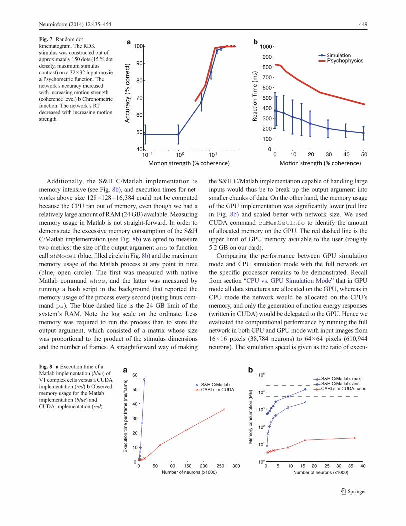
Choice accuracy and RT as a function of task difficulty(coherence of dot motion) are shown in Fig. 7 (Panel a and b,respectively), where the thick red lines are human behavioraldata extracted from a RTexperiment (see Fig. 3 and Table 2 inRoitman and Shadlen (2002)) and simulated data is shown inblue. Each data point (blue) is the mean outcome of 80 trials(fixed coherence level, ten repetitions per motion direction),and the vertical bars are the standard error and standarddeviation for accuracy (Panel a) and RT (Panel b),

respectively. As in Fig. 3 in Roitman and Shadlen (2002),we did not show RTs on error trials.

Our network performance is comparable to human accura-cy, and it qualitatively emulates the effect of motion strengthon RT. Decreasing RT for a relatively easy task (e.g., highmotion coherence) is a direct consequence of the race model.Conversely, when the difficulty of a decision is high (e.g., lowcoherence level), information favoring a particular responsegrows more slowly (Smith and Ratcliff 2004), and the prob-ability of making an error is higher (Shadlen and Newsome2001). The quantitative difference between behavioral andsimulated RT in Fig. 7 could be eradicated by fine-tuningthe excitatory weights from MT cells to the decision layer.However, such an exercise would be meaningless, becauseour model does not take into consideration neural areas in-volved in characteristics of the decision-making process thatinfluence the length of RT, such as the time-course of LIPneuronal dynamics or the gating of saccadic eye movements(Shadlen and Newsome 2001), which have been successfullymodeled in detail by others (Grossberg and Pilly 2008).

Computational Performance

In order to compare our CUDA implementation of V1 (that is,the file v1colorME.cu) to the original, unmodified S&Himplementation (which features code in both C and Matlab)we computed V1 complex cell responses (see section“Spatiotemporal-Energy Model of V1”) at a single spatiotem-poral scale to a drifting sinusoidal grating (the same stimulusas described in section “Direction Tuning”) and recorded themodel’s execution time. The S&H C/Matlab code was exe-cuted as shModel(stim,pars,‘v1Complex’), wherestim was the input stimulus, and pars were the defaultparameters (shPars). Figure 8a shows the execution timeper video frame for both models. Our GPU implementation(red) was not only faster (except for relatively small networks)than the S&H C/Matlab implementation (blue), but it alsoscaled better with network size. Note that the C/Matlab im-plementation was a single-threaded computation. The largestspeedup, a factor of 12, was observed for a network consistingof 96×96=9,216 neurons. It is likely that even greaterspeedups could have been achieved on larger networks, butthese networks could not run with the S&H C/Matlab imple-mentation because they ran out of memory. Timing wasperformed using standard commands tic and toc inMatlab, and the <ctime> function time in C++/CUDA.For the S&H C/Matlab implementation, the time it took tocreate the stimulus was not included in the time measurement.On the other hand, in the CUDA implementation the stimulushad to be read from file frame-by-frame and copied to theGPU card. However, we did not include the time it takes totransfer the response back from the device to the host.

448 Neuroinform (2014) 12:435–454

Additionally, the S&H C/Matlab implementation ismemory-intensive (see Fig. 8b), and execution times for net-works above size 128×128=16,384 could not be computedbecause the CPU ran out of memory, even though we had arelatively large amount of RAM (24GB) available.Measuringmemory usage in Matlab is not straight-forward. In order todemonstrate the excessive memory consumption of the S&HC/Matlab implementation (see Fig. 8b) we opted to measuretwo metrics: the size of the output argument ans to functioncall shModel (blue, filled circle in Fig. 8b) and the maximummemory usage of the Matlab process at any point in time(blue, open circle). The first was measured with nativeMatlab command whos, and the latter was measured byrunning a bash script in the background that reported thememory usage of the process every second (using linux com-mand ps). The blue dashed line is the 24 GB limit of thesystem’s RAM. Note the log scale on the ordinate. Lessmemory was required to run the process than to store theoutput argument, which consisted of a matrix whose sizewas proportional to the product of the stimulus dimensionsand the number of frames. A straightforward way of making

the S&H C/Matlab implementation capable of handling largeinputs would thus be to break up the output argument intosmaller chunks of data. On the other hand, the memory usageof the GPU implementation was significantly lower (red linein Fig. 8b) and scaled better with network size. We usedCUDA command cuMemGetInfo to identify the amountof allocated memory on the GPU. The red dashed line is theupper limit of GPU memory available to the user (roughly5.2 GB on our card).

Comparing the performance between GPU simulationmode and CPU simulation mode with the full network onthe specific processor remains to be demonstrated. Recallfrom section “CPU vs. GPU Simulation Mode” that in GPUmode all data structures are allocated on the GPU, whereas inCPU mode the network would be allocated on the CPU’smemory, and only the generation of motion energy responses(written in CUDA) would be delegated to the GPU. Hence weevaluated the computational performance by running the fullnetwork in both CPU and GPU mode with input images from16×16 pixels (38,784 neurons) to 64×64 pixels (610,944neurons). The simulation speed is given as the ratio of execu-

10−1 100 10140

50

60

70

80

90

100

Acc

urac

y (%

cor

rect

)

0 10 20 30 40 500

100

200

300

400

500

600

700

800

900

1000

Psychophysics

a bFig. 7 Random dotkinematogram. The RDKstimulus was constructed out ofapproximately 150 dots (15 % dotdensity, maximum stimuluscontrast) on a 32×32 input moviea Psychometric function. Thenetwork’s accuracy increasedwith increasing motion strength(coherence level) b Chronometricfunction. The network’s RTdecreased with increasing motionstrength

0 50 100 150 200 250 3000

10

20

30

40

50

60

S&H C/MatlabCARLsim CUDA

100

101

102

103

104

105

S&H C/Matlab: maxS&H C/Matlab: ansCARLsim CUDA: used

0 5 10 15 20 25 30 35 40Number of neurons (x1000) Number of neurons (x1000)

a b

Exe

cutio

n tim

e pe

r fr

ame

(ms/

fram

e)

Mem

ory

cons

umpt

ion

(MB

)

Fig. 8 a Execution time of aMatlab implementation (blue) ofV1 complex cells versus a CUDAimplementation (red) b Observedmemory usage for the Matlabimplementation (blue) andCUDA implementation (red)

Neuroinform (2014) 12:435–454 449

tion time over the simulation time (see Fig. 9a) for networksrun in CPU mode (blue) and GPU mode (red). Note that inboth modes, the V1 CUDA implementation was executed(green), whose run-time is part of the total simulation time(in blue and red). The GPU simulations not only ran faster, butalso simulation speed scaled better with network size. Notethat the CPU simulation was a single-threaded computation.The full network at 40×40 input resolution (239,040 neurons)ran in real-time on the GPU. At 32×32 input resolution(153,216 neurons) the simulation was 1.5 times faster thanreal-time. This result compares favorably with previous re-leases of our simulator (Nageswaran et al. 2009; Richert et al.2011), which is partly due to code-level optimizations, butmostly due to differences in GPU hardware and the V1 stageof the network being spatiotemporal filters instead of spikingneurons. As the network size increased, the GPU simulationsshowed a significant speedup over the CPU (see Fig. 9b).Speedup was computed as the ratio of CPU to GPU executiontime. The largest network we could fit on a single GPUroughly corresponded to 64×64 input resolution (610,944neurons), which ran approximately 30 times faster than onthe CPU. Larger networks currently do not fit on a single GPUand as such must be run on the CPU, which would be morethan 70 times slower than real-time judging from Fig. 9a.

Discussion

We presented a large-scale spiking model of visual area MTthat 1) is capable of exhibiting both component and patternmotion selectivity, 2) generates speed tuning curves that are inagreement with electrophysiological data, 3) reproduces be-havioral responses from a 2AFC task, 4) outperforms a pre-vious rate-based implementation of the motion energy model(Simoncelli and Heeger 1998) in terms of computational

speed and memory usage, 5) is implemented on a publiclyavailable SNN simulator that allows for real-time executionon off-the-shelf GPUs, and 6) is comprised of a neuronmodel,synapse model, and address-event representation (AER),which is compatible with recent neuromorphic hardware(Srinivasa and Cruz-Albrecht 2012).

The model is based on two previous models of motionprocessing in MT (Simoncelli and Heeger 1998; Rust et al.2006), but differs from these models in several ways. First, ourmodel contains the tuned normalization in the MT stage thatwas not present in Simoncelli and Heeger (1998) but intro-duced by Rust et al. (2006). Second, the implementation byRust et al. (2006) was restricted to inputs that are mixtures of12 sinusoidal gratings of a fixed spatial and temporal frequen-cy, whereas our model can operate on any spatiotemporalimage intensity. Third, MT PDS cells in our model sum overinputs fromMTCDS cells as opposed to inputs fromV1 cells,although the two approaches are conceptually equivalent.Fourth, instead of using linear summation and a static nonlin-ear transformation, all neuronal and synaptic dynamics in ourmodel MT were achieved using Izhikevich spiking neuronsand conductance-based synapses.

One could argue that the inclusion of Izhikevich spikingneurons and conductance-based synapses is unnecessary,since previous incarnations of the motion energy model didnot feature these mechanisms yet were perfectly capable ofreproducing speed tuning and motion selectivity. However,our approach is to be understood as a first step into modelinglarge-scale networks of visual motion processing in morebiological detail, with the ultimate goal of understandinghow the brain solves the aperture problem, among other openissues in motion perception. Integrating the functionality dem-onstrated in previous models with more neurobiologicallyplausible neuronal and synaptic dynamics is a necessary firststep into analyzing the temporal dynamics of model neurons

0 200 400 60010−2

10 -1

10 0

10 1

10 2

Number of neurons (x1000)

Exe

cutio

n T

ime

/ Sim

ulat

ion

Tim

e (s

)

0 200 400 60012

14

16

18

20

22

24

26

28

30

Number of neurons (x1000)

GP

U/C

PU

Spe

edup

ba

CPU modeGPU modeV1 CUDA only

Fig. 9 a Simulation speed isgiven as the ratio of executiontime over the simulation time fornetworks run in CPU mode (blue)and GPU mode (red). In bothcases, the V1 CUDAimplementation was executed(green), which is part of the totalsimulation time (in blue and red).Note the log scale on the ordinate.The GPU simulations did not onlyrun faster, but simulation speedscaled better with network size bSpeedup is given as the ratio ofCPU execution time over GPUexecution time

450 Neuroinform (2014) 12:435–454

in MT, which may 1) help to explain how MT PDS cellestablish their pattern selectivity not instantly but over atime-course on the order of 100 ms (Smith et al. 2005) and2) enable the addition of spike-based learning rules such asSTDP; both of which might be harder to achieve with previ-ous model incarnations. Additionally, the introduction of thepresent neuron model, synapse model, and address-event rep-resentation (AER) did not affect performance, yet enabled theintegration of the S&Hmodel with recent neuromorphic hard-ware (Srinivasa and Cruz-Albrecht 2012) (see also section“Practical Implications”).

On the other hand, it is possible (if not likely) that someresponse dynamics produced by the neural circuitry in theretina, the lateral geniculate nucleus (LGN), and V1 mayaccount for certain response properties of neurons in MT.Thus future work could be directed towards implementingthe entire early visual system in the spiking domain.However, for the purpose of this study we deem a rate-basedpreprocessor to be an adequate abstraction, as the core func-tionality of directionally selective cells in V1 seem to be well-characterized by local motion energy filters (Adelson andBergen 1985; DeAngelis et al. 1993; Movshon andNewsome 1996).

Neurophysiological Evidence and Model Alternatives

There is evidence that MT firing rates represent the velocity ofmoving objects using the IOC principle. A psychophysicalstudy showed that the perception of moving plaids depends onconditions that specifically affect the detection of individualgrating velocities (Adelson and Movshon 1982). This is con-sistent with a two-stage model in which component velocitiesare first detected and then pooled to compute pattern velocity.Subsequent physiological studies broadly support such a cas-cade model (Perrone and Thiele 2001; Rust et al. 2006; Smithet al. 2005).

However, other psychophysical results exist where theperceived direction of plaid motion deviates significantly fromthe IOC direction (Ferrera and Wilson 1990; Burke andWenderoth 1993). Alternatives to the IOC principle are, forexample, vector average (VA) or feature tracking. VA predictsthat the perceived pattern motion is the vector average of thecomponent velocity vectors. Blob or feature tracking is theprocess of locating something (a “feature”) that does not sufferfrom the aperture problem, such as a bright spot or a T-junction, and tracking it over time (Wilson et al. 1992).Ultimately, one needs to consider the interactions of the mo-tion pathway with form mechanisms (Majaj et al. 2007), andmodel the processing of more complex stimuli (e.g., motiontransparency, additional self-motion, multiplemoving objects)(Raudies et al. 2011; Layton et al. 2012). Clarifying by whichrule (or combination of rules) the brain integrates motion

signals is still a field of ongoing research. For recent reviewson the topic see (Bradley and Goyal 2008; Nishida 2011).

Although clear evidence for spatiotemporal frequency in-separability in MT neurons has been found (Perrone andThiele 2001), which supports the idea of a motion energymodel, later studies reported it to be a weak effect (Priebeet al. 2003, 2006). The actual proportion of neurons in theprimate visual system that are tuned to spatiotemporal fre-quency is currently not known.

Model Limitations

Although our model is able to capture many attributes ofmotion selectivity (e.g., direction selectivity, speed tuning,component and pattern motion), it is not yet complete for thefollowing reasons. First, it does not explicitly specify the exactpattern velocity, but instead reports an activity distributionover the population of MT neurons, whose firing rates areindicative of the observed pattern motion. In order to estimatethe speed of a target stimulus, it has been proposed to use asuitable population decoding mechanism that operates on MTresponses (Perrone 2012; Hohl et al. 2013). Second, ourmodel does not attempt to predict the temporal dynamics ofMT PDS cells, which often respond with broad selectivitywhen first activated, sometimes even resembling CDS cells,and only over a time-course on the order of 100 ms establishtheir pattern motion selectivity (Smith et al. 2005). A possibleexplanation for these temporal dynamics is given in Cheyet al. (1997). Third, it does not consider the visual formpathway and abstracts early visual details that may be criticalfor operation in natural settings. Fourth, the extent to whicheach stage in the motion energy model can be mapped ontospecific neuronal populations is rather limited. Tiling thespatiotemporal frequency space according to the motion en-ergy model is biologically implausible, and the temporalextent of the filters is unrealistically long (especially the lowspeed filters). However, a way to combine spatiotemporalfilters based on V1 neuron properties into a pattern motiondetector has been proposed in Perrone and Thiele (2002).

Another more fundamental limitation is that the S&Hmodel (or for that matter, any spatiotemporal-energy basedmodel including the elaborated Reichardt detector) can onlysense so-called first-order motion, which is defined as spatio-temporal variations in image intensity (first-order imagestatistics) that give rise to a Fourier spectrum. Second-orderstimuli, such as the motion of a contrast modulation over atexture, are non-Fourier and thus invisible to the model, yetcan be readily perceived by humans (Chubb and Sperling1988). In addition, the existence of a third motion channelhas been suggested, which is supposed to operate throughselective attention and saliency maps (Lu and Sperling1995). Also, MT has been shown to be involved in color-based motion perception (Thiele et al. 2001).

Neuroinform (2014) 12:435–454 451

There is also a plainly technical limitation to our model,which is manifested in the amount of available GPU memory.Due to their size, large-scale spiking networks have demand-ing memory requirements. The largest network that could fiton a single NVIDIATeslaM2090 (with 6 GB ofmemory) wascomprised of 610,944 neurons and approximately 137 millionsynapses, which corresponds to processing a 64×64 inputvideo. In order to run larger networks on current-generationGPU cards, a change in model (or software and hardware)architecture is required. One should note that this is only atemporary limitation and could become obsolete as soon aswith the next generation of GPU cards. Another possiblesolution would be to employ multi-GPU systems; however,more work is required to efficiently integrate our SNN simu-lator with such a system.

Practical Implications

The present network might be of interest to the neuroscientistand computer vision research communities for the followingreasons.

First, our implementation outperforms the S&H C/Matlabimplementation by orders of magnitude in terms of computa-tional speed and memory usage. Thus our CUDA implemen-tation can be used to save computation time, as well as beapplied to input resolutions that the C/Matlab implementationcannot handle due to memory constraints. Additionally, theCUDA implementation can act as a stand-alone module thatcould potentially be used in computer vision as an alternativeto computationally expensive operations such as Gabor filter-ing for edge detection or dense optic flow computations.

Second, we have demonstrated that our approach is fast,efficient, and scalable; although current GPU cards limit thesize of the simulations due to memory constraints.Nevertheless, our model processes a 40×40 input video at20 frames per second in real-time, which corresponds to a totalof 239,040 neurons in the simulated V1,MT, and LIP areas, at20 frames per second using a single GPU, which enables thepotential use of our software in real-time applications rangingfrom robot vision to autonomous driving.

Third, our implementation might be of particular interest tothe neuromorphic modeling community, as the present neuronmodel, synapse model, and AER are compatible with recentneuromorphic hardware (Srinivasa and Cruz-Albrecht 2012).Thus our algorithm could be used as a neural controller inneuromorphic and neurorobotics applications. Future workcould be directed toward creating an interface by which net-works can be automatically exported onto neuromorphichardware.

Fourth, because of the modular code structure, our imple-mentation can be readily extended to include, for example,higher-order visual areas or biologically plausible synapticlearning rules such as STDP. Thus our implementation may

facilitate the testing of hypotheses and the study of the tem-poral dynamics that govern visual motion processes in areaMT, which might prove harder to study using previous (rate-based) model incarnations.

Lastly, the network was constructed using a SNN simulatorthat is publicly available at http://www.socsci.uci.edu/~jkrichma/CARLsim/. The present release features thecomplete source code for the simulator, the network, andanalysis scripts. As such it is the next step towards our goalof making efficient simulations of large-scale spiking net-works available to a wide range of researchers, without theneed of a cluster or supercomputer.

Information Sharing Statement

The source code for the simulator, for the network, and anal-ysis scripts are publicly available at http://www.socsci.uci.edu/~jkrichma/CARLsim/. This website does also featureinstallation instructions, source code documentation and atutorial on how to set up, run, and interact with a simulation.In order to run the simulator in CUDA mode, the NVIDIACUDA software developer kit must be installed (freeware,available at https://developer.nvidia.com/cuda-downloads).

Acknowledgments This work was supported by the Defense Ad-vanced Research Projects Agency (DARPA) subcontract 801888-BS.We thank Jayram M. Nageswaran for his work developing the customspiking neural network simulator. We also thank Michael Avery, KrisCarlson, and Steve Grossberg for valuable feedback and discussion onthis project.

Conflict of Interest The authors have no conflicts of interest with thismanuscript.

References

Adelson, E. H., & Bergen, J. R. (1985). Spatiotemporal energymodels forthe perception of motion. Journal of the Optical Society of AmericaA, 2(2), 284–299.

Adelson, E. H., & Movshon, J. A. (1982). Phenomenal coherence ofmoving visual patterns. Nature, 300(5892), 523–525.

Bradley, D. C., & Goyal, M. S. (2008). Velocity computation in theprimate visual system. Nature Reviews Neuroscience, 9(9), 686–695. doi:10.1038/Nrn2472.

Browning, N. A., Grossberg, S., & Mingolla, E. (2009a). Cortical dy-namics of navigation and steering in natural scenes: motion-basedobject segmentation, heading, and obstacle avoidance. NeuralNetworks, 22(10), 1383–1398. doi:10.1016/j.neunet.2009.05.007.

Browning, N. A., Grossberg, S., & Mingolla, E. (2009b). A neural modelof how the brain computes heading from optic flow in realisticscenes. Cognitive Psychology, 59(4), 320–356. doi:10.1016/j.cogpsych.2009.07.002.

Burke, D., & Wenderoth, P. (1993). The effect of interactions betweenone-dimensional component gratings on 2-dimensional motion per-ception. Vision Research, 33(3), 343–350. doi:10.1016/0042-6989(93)90090-J.

452 Neuroinform (2014) 12:435–454

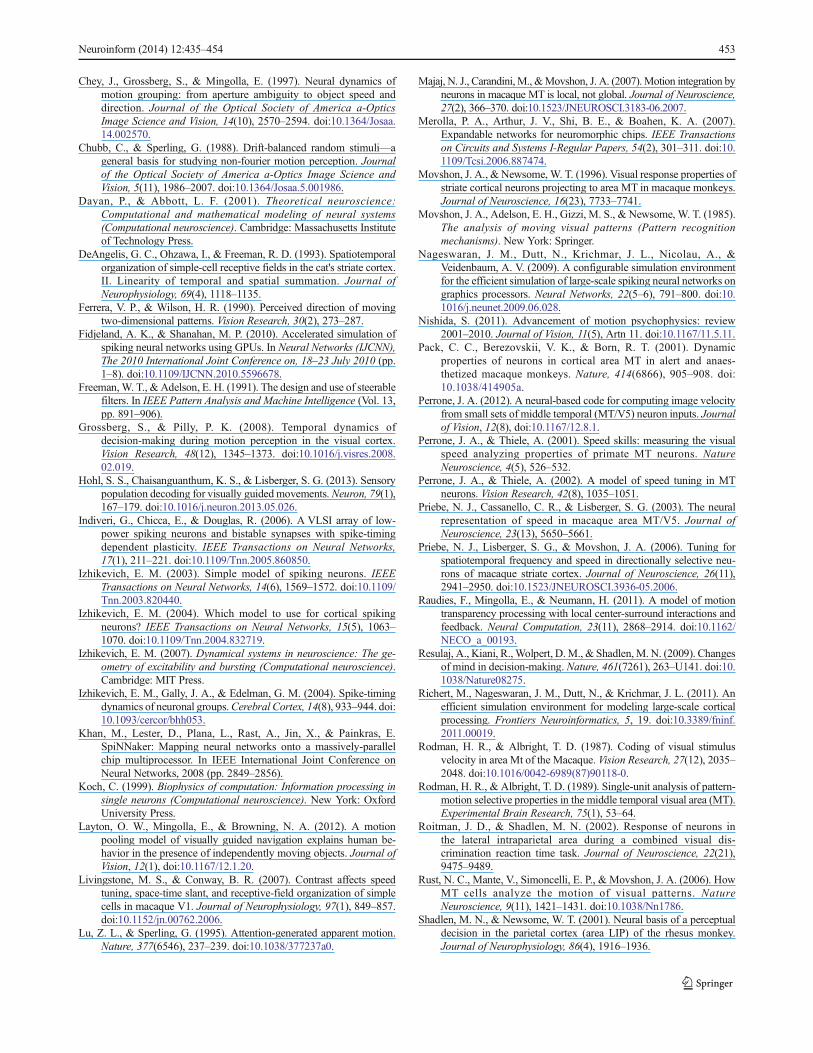
Chey, J., Grossberg, S., & Mingolla, E. (1997). Neural dynamics ofmotion grouping: from aperture ambiguity to object speed anddirection. Journal of the Optical Society of America a-OpticsImage Science and Vision, 14(10), 2570–2594. doi:10.1364/Josaa.14.002570.

Chubb, C., & Sperling, G. (1988). Drift-balanced random stimuli—ageneral basis for studying non-fourier motion perception. Journalof the Optical Society of America a-Optics Image Science andVision, 5(11), 1986–2007. doi:10.1364/Josaa.5.001986.

Dayan, P., & Abbott, L. F. (2001). Theoretical neuroscience:Computational and mathematical modeling of neural systems(Computational neuroscience). Cambridge: Massachusetts Instituteof Technology Press.

DeAngelis, G. C., Ohzawa, I., & Freeman, R. D. (1993). Spatiotemporalorganization of simple-cell receptive fields in the cat's striate cortex.II. Linearity of temporal and spatial summation. Journal ofNeurophysiology, 69(4), 1118–1135.

Ferrera, V. P., & Wilson, H. R. (1990). Perceived direction of movingtwo-dimensional patterns. Vision Research, 30(2), 273–287.

Fidjeland, A. K., & Shanahan, M. P. (2010). Accelerated simulation ofspiking neural networks using GPUs. In Neural Networks (IJCNN),The 2010 International Joint Conference on, 18–23 July 2010 (pp.1–8). doi:10.1109/IJCNN.2010.5596678.

Freeman,W. T., & Adelson, E. H. (1991). The design and use of steerablefilters. In IEEE Pattern Analysis and Machine Intelligence (Vol. 13,pp. 891–906).

Grossberg, S., & Pilly, P. K. (2008). Temporal dynamics ofdecision-making during motion perception in the visual cortex.Vision Research, 48(12), 1345–1373. doi:10.1016/j.visres.2008.02.019.

Hohl, S. S., Chaisanguanthum, K. S., & Lisberger, S. G. (2013). Sensorypopulation decoding for visually guided movements.Neuron, 79(1),167–179. doi:10.1016/j.neuron.2013.05.026.

Indiveri, G., Chicca, E., & Douglas, R. (2006). A VLSI array of low-power spiking neurons and bistable synapses with spike-timingdependent plasticity. IEEE Transactions on Neural Networks,17(1), 211–221. doi:10.1109/Tnn.2005.860850.

Izhikevich, E. M. (2003). Simple model of spiking neurons. IEEETransactions on Neural Networks, 14(6), 1569–1572. doi:10.1109/Tnn.2003.820440.

Izhikevich, E. M. (2004). Which model to use for cortical spikingneurons? IEEE Transactions on Neural Networks, 15(5), 1063–1070. doi:10.1109/Tnn.2004.832719.

Izhikevich, E. M. (2007). Dynamical systems in neuroscience: The ge-ometry of excitability and bursting (Computational neuroscience).Cambridge: MIT Press.

Izhikevich, E. M., Gally, J. A., & Edelman, G. M. (2004). Spike-timingdynamics of neuronal groups.Cerebral Cortex, 14(8), 933–944. doi:10.1093/cercor/bhh053.

Khan, M., Lester, D., Plana, L., Rast, A., Jin, X., & Painkras, E.SpiNNaker: Mapping neural networks onto a massively-parallelchip multiprocessor. In IEEE International Joint Conference onNeural Networks, 2008 (pp. 2849–2856).

Koch, C. (1999). Biophysics of computation: Information processing insingle neurons (Computational neuroscience). New York: OxfordUniversity Press.

Layton, O. W., Mingolla, E., & Browning, N. A. (2012). A motionpooling model of visually guided navigation explains human be-havior in the presence of independently moving objects. Journal ofVision, 12(1), doi:10.1167/12.1.20.

Livingstone, M. S., & Conway, B. R. (2007). Contrast affects speedtuning, space-time slant, and receptive-field organization of simplecells in macaque V1. Journal of Neurophysiology, 97(1), 849–857.doi:10.1152/jn.00762.2006.

Lu, Z. L., & Sperling, G. (1995). Attention-generated apparent motion.Nature, 377(6546), 237–239. doi:10.1038/377237a0.

Majaj, N. J., Carandini, M., &Movshon, J. A. (2007).Motion integration byneurons in macaque MT is local, not global. Journal of Neuroscience,27(2), 366–370. doi:10.1523/JNEUROSCI.3183-06.2007.

Merolla, P. A., Arthur, J. V., Shi, B. E., & Boahen, K. A. (2007).Expandable networks for neuromorphic chips. IEEE Transactionson Circuits and Systems I-Regular Papers, 54(2), 301–311. doi:10.1109/Tcsi.2006.887474.

Movshon, J. A., & Newsome, W. T. (1996). Visual response properties ofstriate cortical neurons projecting to area MT in macaque monkeys.Journal of Neuroscience, 16(23), 7733–7741.

Movshon, J. A., Adelson, E. H., Gizzi, M. S., & Newsome, W. T. (1985).The analysis of moving visual patterns (Pattern recognitionmechanisms). New York: Springer.

Nageswaran, J. M., Dutt, N., Krichmar, J. L., Nicolau, A., &Veidenbaum, A. V. (2009). A configurable simulation environmentfor the efficient simulation of large-scale spiking neural networks ongraphics processors. Neural Networks, 22(5–6), 791–800. doi:10.1016/j.neunet.2009.06.028.

Nishida, S. (2011). Advancement of motion psychophysics: review2001–2010. Journal of Vision, 11(5), Artn 11. doi:10.1167/11.5.11.

Pack, C. C., Berezovskii, V. K., & Born, R. T. (2001). Dynamicproperties of neurons in cortical area MT in alert and anaes-thetized macaque monkeys. Nature, 414(6866), 905–908. doi:10.1038/414905a.

Perrone, J. A. (2012). A neural-based code for computing image velocityfrom small sets of middle temporal (MT/V5) neuron inputs. Journalof Vision, 12(8), doi:10.1167/12.8.1.

Perrone, J. A., & Thiele, A. (2001). Speed skills: measuring the visualspeed analyzing properties of primate MT neurons. NatureNeuroscience, 4(5), 526–532.

Perrone, J. A., & Thiele, A. (2002). A model of speed tuning in MTneurons. Vision Research, 42(8), 1035–1051.

Priebe, N. J., Cassanello, C. R., & Lisberger, S. G. (2003). The neuralrepresentation of speed in macaque area MT/V5. Journal ofNeuroscience, 23(13), 5650–5661.

Priebe, N. J., Lisberger, S. G., & Movshon, J. A. (2006). Tuning forspatiotemporal frequency and speed in directionally selective neu-rons of macaque striate cortex. Journal of Neuroscience, 26(11),2941–2950. doi:10.1523/JNEUROSCI.3936-05.2006.

Raudies, F., Mingolla, E., & Neumann, H. (2011). A model of motiontransparency processing with local center-surround interactions andfeedback. Neural Computation, 23(11), 2868–2914. doi:10.1162/NECO_a_00193.

Resulaj, A., Kiani, R.,Wolpert, D.M., & Shadlen,M. N. (2009). Changesof mind in decision-making. Nature, 461(7261), 263–U141. doi:10.1038/Nature08275.

Richert, M., Nageswaran, J. M., Dutt, N., & Krichmar, J. L. (2011). Anefficient simulation environment for modeling large-scale corticalprocessing. Frontiers Neuroinformatics, 5, 19. doi:10.3389/fninf.2011.00019.

Rodman, H. R., & Albright, T. D. (1987). Coding of visual stimulusvelocity in area Mt of the Macaque. Vision Research, 27(12), 2035–2048. doi:10.1016/0042-6989(87)90118-0.

Rodman, H. R., & Albright, T. D. (1989). Single-unit analysis of pattern-motion selective properties in the middle temporal visual area (MT).Experimental Brain Research, 75(1), 53–64.

Roitman, J. D., & Shadlen, M. N. (2002). Response of neurons inthe lateral intraparietal area during a combined visual dis-crimination reaction time task. Journal of Neuroscience, 22(21),9475–9489.

Rust, N. C., Mante, V., Simoncelli, E. P., & Movshon, J. A. (2006). HowMT cells analyze the motion of visual patterns. NatureNeuroscience, 9(11), 1421–1431. doi:10.1038/Nn1786.

Shadlen, M. N., & Newsome, W. T. (2001). Neural basis of a perceptualdecision in the parietal cortex (area LIP) of the rhesus monkey.Journal of Neurophysiology, 86(4), 1916–1936.

Neuroinform (2014) 12:435–454 453

Simoncelli, E. P., & Heeger, D. J. (1998). A model of neuronal responsesin visual area MT. Vision Research, 38(5), 743–761. doi:10.1016/S0042-6989(97)00183-1.

Smith, P. L., & Ratcliff, R. (2004). Psychology and neurobiology ofsimple decisions. Trends in Neurosciences, 27(3), 161–168. doi:10.1016/j.tins.2004.01.006.

Smith, M. A., Majaj, N. J., & Movshon, J. A. (2005). Dynamics ofmotion signaling by neurons in macaque area MT. NatureNeuroscience, 8(2), 220–228. doi:10.1038/Nn1382.

Srinivasa, N., & Cruz-Albrecht, J. M. (2012). Neuromorphic adaptiveplastic scalable electronics analog learning systems. IEEE Pulse,3(1), 51–56. doi:10.1109/Mpul.2011.2175639.

Thiele, A., Dobkins, K. R., & Albright, T. D. (2001). Neuralcorrelates of chromatic motion perception. Neuron, 32(2),351–358.

van Santen, J. P. H., & Sperling, G. (1985). Elaborated Reichardt detec-tors. Journal of the Optical Society of America a-Optics ImageScience and Vision, 2(2), 300–321.

Vogelstein, R. J., Mallik, U., Culurciello, E., Cauwenberghs, G., &Etienne-Cummings, R. (2007). A multichip neuromorphic systemfor spike-based visual information processing.Neural Computation,19(9), 2281–2300. doi:10.1162/neco.2007.19.9.2281.

Wilson, H. R., Ferrera, V. P., & Yo, C. (1992). A psychophysicallymotivated model for 2-dimensional motion perception. VisualNeuroscience, 9(1), 79–97.

Yudanov, D., Shaaban, M., Melton, R., & Reznik, L. (2010). GPU-basedsimulation of spiking neural networks with real-time performance&amp; high accuracy. In Neural Networks (IJCNN), The 2010International Joint Conference on, 18–23 July 2010 (pp. 1–8). doi:10.1109/IJCNN.2010.5596334.

454 Neuroinform (2014) 12:435–454