effects of percent impervious cover on fish and benthos ... · effects of percent impervious cover...

577

Effects of Percent Impervious Cover onFish and Benthos Assemblages and Instream

Habitats in Lake Ontario Tributaries

Les W. Stanfield*Lake Ontario Fisheries Unit, Ontario Ministry of Natural Resources

Picton, Ontario, KOK 2T0, Canada

Bruce W. KilgourStantec Consulting, 1505 Laperriere Avenue

Ottawa, Ontario, K1Z 7T1, Canada

Abstract.—–We demonstrate the effects of percent impervious cover (PIC) on biophysical prop-erties of Lake Ontario tributary streams. Biophysical data (fish assemblages, benthic inverte-brate assemblages (benthos), instream physical habitat, and temperature) were collected frommore than 575 wadeable stream sites. A geographic information system application was devel-oped to characterize the landscape upstream of each site (i.e., drainage area, surficial geology,land use/land cover, slope, stream length, and climate). Total PIC of catchments was estimatedfrom land use/land cover, and a base flow index was derived from the surficial geology. Therelationship between PIC and biophysical responses was determined after statistically remov-ing the effects of natural landscape features (i.e., catchment area, slope, base flow index) onthose responses. Contrasts in PIC from natural conditions (<3% to 10%) were related to varia-tions in fish and benthos assemblages. Both coldwater sensitive and warmwater tolerant fishand diverse benthos assemblages were found in catchments with low PIC. At more than 10PIC (i.e., about 50% urban), both fish and benthos consisted of mainly warmwater or tolerantassemblages. For example, trout were absent and minnows were dominant. While some of theapparent PIC effect may have been confounded by land use/land cover and surficial geology,the consistency of the findings even after natural catchment conditions were considered sug-gests that the threshold response is valid. Percent impervious cover had a weaker effect oninstream geomorphic variables than on biological variables. The models derived from thisstudy can be used to predict stream biophysical conditions for catchments with varying levelsof development.

*Corresponding author: [email protected]

American Fisheries Society Symposium 48:577–599, 2006© 2006 by the American Fisheries Society

INTRODUCTION

Human populations in the Greater Toronto Area(GTA) and central Ontario are predicted to in-crease by nearly 3 million over the next 24 years(Statistics Canada 2003), and urban develop-ment associated with those increases threatensecosystems dependent on the Oak Ridges Mo-raine. Human land use has direct and indirecteffects on physical, chemical, and biological char-

acteristics of streams and has been modeled us-ing a variety of land-use/land-cover descriptors.Metrics such as catchment population density(Jones and Clark 1987), agriculture (Harding etal. 1999), width of riparian zones (Barton et al.1985), and land use/land cover (Kilgour andBarton 1999) have been related to instream bio-logical responses. In general, more intensivedevelopment degrades fish and benthos assem-blages and instream habitats. A quantitative un-derstanding of the relationships betweendevelopment and ecological conditions enables

27stanfield2.p65 4/4/2006, 11:24 AM577

578 Stanfield and Kilgour

planners to predict and mitigate impacts fromfuture land conversions, particularly to ensurethat thresholds are not exceeded that would leadto irreversible damages to the ecosystem.

Percent impervious cover (PIC) is a metricthat integrates various types of human develop-ment activities in catchments. Impervious landsare those that have been covered by materialssuch as concrete, asphalt, and rooftops or resultin severe compaction or draining of the soils, allof which restrict infiltration. Different land cov-ers are variably permeable (impermeable). ThePIC in a catchment is the weighted average im-perviousness for the entire catchment. Percentimpervious cover is typically low in natural land-scapes, intermediate in agricultural landscapes,and high in urban landscapes. Leopold (1968)recognized that the transition from natural for-est cover to agricultural and urban landscapesresulted in increased PIC of the land and led toreduced infiltration of precipitation into soils andincreased overland flow. Streams in disturbedcatchments tended to respond faster and moreseverely to storm events, had lower base flowsduring dry seasons, and were wider, shallower,more polluted, and warmer than streams in un-disturbed catchments (Leopold 1968).

Percent impervious cover is recognized as amaster variable for quantifying both physical andbiological stressors in streams. Shaver andMaxted (1995), demonstrated in Delaware thatpercent Ephemeroptera-Plecoptera-Trichopterataxa (mayflies, stoneflies, caddisflies) was signifi-cantly lower in streams with PIC greater than10%. Klein (1979) demonstrated that fish spe-cies richness declined linearly with PIC such thatcatchments with 30–50% PIC either had severelyimpaired fish assemblages or fish were absent.Several authors have identified impairments tofish metrics at PIC levels greater than 10%. Forexample Steedman (1988) and Wang et al. (2000)both reported that the number of fish speciesand/or an index of biotic integrity (IBI) de-creased in streams above this threshold. Limburgand Schmidt (1990) documented declines in

anadromous fish egg and fry densities above aPIC of 10%. Results for benthos are comparable,although evidence of threshold responses are lessconvincing. Jones and Clark (1987) identified athreshold response at 15% PIC, while Yoder etal. (1999), Shaver and Maxted (1995), and Mayet al. (1997) determined that benthos taxa di-versity declined above 5–8% PIC. Klein (1979)however was unable to identify a threshold re-sponse and suggested that confounding factorssuch as the presence of riparian zones may bufferthe overall effect of PIC on streams. Several stud-ies have confirmed even lower threshold re-sponses to geomorphic variables. Dunne andLeopold (1978) found dramatic change in chan-nel dimensions at only 4% PIC. Booth and Jack-son (1997) found that even at low levels ofeffective impervious cover, flow patterns weresignificantly altered and that by PIC levels of 6–10% PIC, there is a loss of aquatic system func-tion that may be irreversible.

We believe there are three key factors that ex-plain the differences in response to PIC in thesestudies: differences in resilience to PIC betweenecoregions, differences in how instream features(e.g., fish, substrate, etc.) are measured betweenstudies, and differences in how PIC has been es-timated. Until comparisons can be made be-tween ecoregions using similar measures ofinstream conditions and PIC, application of therelationship between PIC and stream conditionmust rely on locally derived models.

Our objective was to quantify the relationshipbetween catchment PIC and biophysical char-acteristics of streams. We recognize that muchof the variability in the biophysical makeup ofstreams is due to natural catchment characteris-tics and the location of the stream within thecatchment. Therefore, we accounted for catch-ment characteristics that might influence streamhydrology and sediments. By including both thebiotic and abiotic properties of streams, we at-tempt to demonstrate how biotic–abiotic rela-tionships can assist managers in predictingchanges from future development scenarios.

27stanfield2.p65 4/4/2006, 11:24 AM578

Effects of Percent Impervious Cover on Fish and Benthos Assemblages and Instream Habitats 579

METHODS

Study Area

Fish, benthic invertebrates, and instream habi-tat conditions were characterized at wadeablesites along the north shore of Lake Ontario. TheOak Ridges Moraine and Niagara Escarpmentdominate this landscape and ensure strong baseflow to streams, which historically provided val-ued salmonid fisheries for the early settlers in theregion (Figure 1). Data were collected 1995–2002by several agencies using methods described inStanfield et al. (1997). Sites were selected usingmultiple stratified random designs. Several stud-ies covered the entire ecoregion. Most studieswere stratified based on a measure of stream size.Sampling intensity and the types of data collected

(not all methods were applied at all sites) withineach stratum were designed to meet the desiredprecision of each study. Once the study designwas determined, sites were randomly selectedwithin each stratum. Sites were a minimum of40 m long, with boundaries at crossovers (i.e.,the location where the thalweg is in the middleof the stream) (Stanfield et al. 1997). In streamsin our study area, this site length provides a reli-able measure of fish biomass (Jones andStockwell 1995), species richness (L. W. Stanfield,unpublished data), and instream habitat(Stanfield and Jones 1998). This design enabledmany more sites to be sampled in a day and pro-vided an opportunity to develop a more robustestimate of fish assemblages within an entirestream than if a single long site (e.g., 40 bank-full widths; Lyons 1992) were sampled.

Figure 1. Major features of the study area and distribution of sample sites.

27stanfield2.p65 4/4/2006, 11:24 AM579


Fish Assemblage Data

Fish were collected by single-pass electrofishingat 721 sites, without bias, for size or species. Ef-fort expended per site varied (4–15 s/m2), butwas sufficient to provide comparable assemblagemeasures at each site (Stanfield, unpublisheddata). All fish were immediately weighed, iden-tified to species, and released, except those keptfor laboratory identification. Mottled sculpinCottus bairdii and slimy sculpin C. cognatus andAmerican brook lamprey Lampetra appendixand sea lamprey Petromyzon marinus were in-consistently identified and were therefore com-bined by genus for this analysis.

Benthos Assemblage Data

Benthos were sampled at 583 sites using a modi-fied version of Plafkin et al. (1989). Two benthossamples were collected from within crossovers,using a 2-min stationary kick-and-sweepmethod, with 1-mm mesh, over approximately1 m2. Organisms were picked from samplingtrays until at least 100 individuals were obtainedfor each replicate or the entire sample was pro-cessed. Benthos were identified to major taxo-nomic groups (see Table 1).

Instream Habitat Data

Instream habitat data were collected from 578sites using a point-transect survey design. De-pending on stream width, from 10 to 20 transects(>3 m width = 10) were established at regular

spacing within each site and then 2–6 observa-tion points (>3 m width = 6) were identified oneach transect. This design explained 90% of thevariability in instream habitat from streamswithin this study area (Stanfield and Jones 1998).At each observation point (total of 40–60/site),depth, substrate, and hydraulic head were mea-sured. Hydraulic head was used as a surrogatefor stream velocity and represents the heightwater climbs a ruler held at right angles to flow.Cover and maximum particle size (largestpresent) were measured within a 30-cm ring thatwas centered on each observation point. Cover(converted to percent) was an object 10 cm wideon its median axis that intersected a 30-cm ring,centered on each observation point. Percent fines(particles � 2 mm) and the D16, D50, and D85were determined from substrate particle sizemeasurements. Proportions of 16 categories ofmorphological features were determined basedon the classes of depth (10, 60, 100 and >100cm) and hydraulic head (<3, 4–7, 8–17, and >17mm) at each observation point. A measure ofchannel homogeneity was determined by sum-ming the proportion of a site within one categoryof the dominant morphologic feature at the site.The width-to-depth ratio was determined byaveraging the sum of the wetted width to depthratios of each transect.

Four metrics were calculated to provide mea-sures of channel stability (Table 2). The vulner-ability to erosion for streambanks wasdetermined at each bank intercepted at a trans-ect. Field measurements of bank angle, bank ma-terial, presence of undercuts, rooted vegetation

Table 1. Benthos taxa identified, and adjusted ratings used to calculate the Hilsenhoff biotic index score.Ratings based on a review of the original ratings of families common to southern Ontario.

Taxa Rating Taxa Rating Taxa Rating

Hydracarina 6 Amphipoda 6 Simuliidae 6Oligochaeta 8 Isopoda 8 Other Diptera 5Hirudinea 8 Chironomidae 7 Tipulidae 3Hemiptera 5 Coleoptera 4 Megaloptera 4Anisoptera 5 Zygoptera 7 Trichoptera 4Gastropoda 8 Pelecypoda 8 Ephemeroptera 5Decapoda 6 Plecoptera 1 Ostracoda 7

27stanfield2.p65 4/4/2006, 11:24 AM580


and riparian vegetation type were interpretedwith a dichotomous key. Bank height informa-tion and substrate size at four horizontal dis-tances (0, 0.25, 0.75, and 1.5 m) from the streamedge were used to determine whether the bankangle exceeded 45° and consisted of erodiblematerial. Undercuts more than 5 cm deep wererecorded, and the percent of rooted vegetativecover in the first 1 m of bank was measured bycounting the number of squares in a grid occu-pied by live vegetation. Finally, the dominantvegetative type in a 2-m2 grid at the intersectionof each transect was recorded. Bank ratingsranged from 0.2 (e.g., undercut present and noforest cover present) to 1.0 (e.g., no undercutpresent, bank angle less than 45% and greaterthan 70% of squares with root cover). The coef-ficient of variation for the maximum particleswas used as a measure of sediment sorting at eachsite. Sediment transport potential was estimatedby dividing the D50 for the point and maximumparticle sizes. Channel stability for each site rep-resented the cumulative ratings for the fourmetrics (Table 2).

Stream Temperature Data

Water temperatures were recorded at 622 sites,between 1600 hours and 1700 hours, during low-flow conditions (mid-July to mid-September),when the daily air temperature exceeded 24°Cfor three consecutive days. We standardizedstream temperatures for each site as follows. The

observed water and air temperatures were usedto classify each site as either cold, cool, or warmusing the nomogram developed by Stonemanand Jones (1996). The appropriate regression line(Table 3) was used to predict the stream tem-perature at an air temperature of 30°C. Finally,the difference between the observed and pre-dicted temperature was added to the predictedtemperature at 30°C to obtain the standardizedstream temperature at 30°C for each site. Forexample, if a stream temperature of 25°C wasdetermined at an air temperature of 27°C, itwould be classified as warm. This site is 1.2°Cwarmer than predicted from the algorithm for awarmwater stream (Table 3), and therefore, thestandardized stream temperature would be26.7°C:

standardized temperature = (30*0.555 +8.838) + (25–23.8). [1]

Table 2. Criteria used to score metrics used to create an overall rating of channel stability for each site. Resultsfrom field surveys derived summary statistics for each metric. Ratings were developed based on the relativeimportance of each metric as a measure of channel stability and thresholds for each metric were based onresults of local geomorphic studies (John Parish, Parish Geomorphic, personal communication). Final score forchannel stability was the cumulative ratings from the four metrics

Ratings

Metric 0 0.1 0.2 0.3

Width/depth >60 >40 � 60 >20 � 40 <20Bank stability �0.4 >0.4 � 0.59 >0.6 � 0.79 >0.8Sediment sorting �70 > 70 � 120 >120Sediment transport >36 >12 � 36 �12

Table 3. Regression parameters used to predict watertemperatures from air temperatures for referencestream types. Sites were assigned a reference classbased on the lowest deviation from the observed andthe predicted water temperature for the air tempera-ture on the day of collection.

Reference Class Slope Constant

Cold 0.251 7.513Cool 0.583 3.497Warm 0.555 8.838

27stanfield2.p65 4/4/2006, 11:24 AM581


Landscape Data

Landscape variables were generally derived forthe total catchment, through use of a geographi-cal information systems application, followingStanfield and Kuyvenhoven (2003). Measured at-tributes from a 1:10,000 DEM with 25-m resolu-tion included drainage area, link number,elevation, stream length, and site slope (deter-mined from elevations at 100 m up and down-stream of each site). The Ontario Ministry ofNatural Resources developed a land cover GISlayer at 1:10,000 that assigns 1 of 28 classes to each25-m pixel. Land classifications were based oninterpretation of Landsat imageries collected from1995 and 1996. From this classification, we quan-tified the amount of forest, urban, pasture, inten-sive agriculture (row crops and orchard), andwater (lake, river, and wetland) in each catchment.

The area covered by each class of quaternarysurficial geology (1:250,000) (Ontario Geologi-cal Survey 1997) was determined for each catch-ment. A base flow index (BFI) for each site wasderived from relationships demonstrated byPiggott et al. (2002) between this index and baseflow (Table 4). The BFI was calculated by sum-ming the ranked percentage of each quaternarysurficial geology unit for each catchment:

BFI per site =�ij(%geology typei*BFI ratingi)j [2]

Impervious ratings for each land-use/land-cover category were selected based on an under-standing of how closely the land-cover categoriesrelated to published ratings. Intensive agricul-ture and pasture lands are typically both ratedlow and similarly (i.e., 0.02, NCDE 2002, 2003;and 0.094, Prisloe et al. 2001). We chose to splitthese categories and rate intensive agriculturehigher (0.10) than pasture lands (0.05) becausein our study area, intensive agriculture often in-volves tile drainage and compaction from heavymachinery. Urban land ratings vary considerablydepending on the detail available from the basedata: 0.23–0.86 (NCDE 2002), 0.10–0.38 (NCDE2003), 0.12–0.51 (Prisloe et al. 2001), and 0.20–0.95 (Arnold and Gibbons 1996). We chose aconservative rating of 0.20 for urban lands be-cause of the coarseness of our land-use/land-cover data. Forested lands (0.01) and water/wetlands (0.0) were both given low ratings.

A rating for catchment percent imperviouscover (PIC) was estimated as the sum of theproducts of percent cover by each land-use/land-cover class and the associated impervious ratingof each class. An upstream catchment area with25% water, 25% intensive agriculture, and 50%urban area, for example, would have a PIC of12.5 (i.e., 0 × 25% + 0.1 × 25% + 0.2 × 50%).

Data Analysis

The objective of the data analysis was todetermine if attributes of fish and benthos as-semblages and instream physical habitat char-acteristics were related to PIC, after accountingfor natural landscape influences. Fish assemblagemetrics included total biomass (g/m2) and spe-cies richness, while a modified Hilsenhoff bioticindex (HBI; Hilsenhoff 1987) and taxa richnesswere calculated for the benthos assemblage. Bothbenthos metrics were based on higher level tax-onomy, and as such, the HBI ratings were as-signed based on a review of the original scores

Table 4. Baseflow index (BFI) ratings for quaternarygeology classes from the Ontario geological survey(1997) (Source: Piggott et al. 2002).

Geology type BFI rating

Bedrock (Paleozoic) 0.4Tavistock Till (Huron - Georgian Bay lobe) 0.29Port Stanley Till (Ontario - Erie lobe) 0.27Newmarket Till ( Simcoe lobe) 0.43Wentworth Till (Ontario - Erie lobe) 0.68Kettleby Till (Simcoe lobe) 0.38Halton Till (Ontario - Erie lobe) 0.39Clay till 0.28Till 0.4Glaciofluvial ice-contact deposits 0.67Glaciofluvial outwash deposits 0.77Glaciolacustrine deposits 0.14Glaciolacustrine deposits 0.77Fluvial deposits 0.38Organic deposits 0.35

27stanfield2.p65 4/4/2006, 11:24 AM582


for lower taxa developed by Hilsenhoff (1987;Table 1).

Correspondence analysis (CA) was used sepa-rately for fish and benthos assemblages to evalu-ate assemblage composition. Correspondenceanalysis ordination calculates a set of “synthetic”variables (axes) that best explain variations intaxa abundances across samples. Calculation ofsample and taxa scores on the first ordinationaxis is done by iteratively estimating theweighted-average sample scores and theweighted average taxa scores. For the first itera-tion, axis scores are arbitrarily assigned to eachtaxon. For each sample, the procedure deter-mines the weighted-average axis score, which isthe average of the taxa scores weighted by theabundances of each taxon. The next iterationproduces new weighted average axis scores forthe taxa, calculated from the sample scores. Theiterative procedure continues until there is littlechange in the sample and taxa scores. Estima-tion of second and third ordination axes followsa similar routine, except that the sample scoresof additional axes are orthogonal (uncorrelated)with the first and subsequent axes. Sample scoresin CA are usually scaled to a mean of zero andstandard deviation of 1 (ter Braak 1992). Thedistribution of samples in a CA diagram indi-cates the relative similarities and differences incomposition based on taxa abundances. Siteswith similar scores have taxa in similar propor-tions. The scatter diagram for taxa portrays thedispersion of taxa along the theoretical variables(axes). Thus, a sample with an axis-1 score of 2would be dominated by taxa that also had axis-1scores close to 2. With CA, the configuration ofordination diagrams tends to be sensitive to raretaxa (Gauch 1982). Therefore, we retained foranalysis only those taxa found in more than 5%of sites.

Canonical correspondence analysis (CCA; terBraak 1992) was used to illustrate how fish andbenthos assemblages varied with landscape at-tributes. Canonical correspondence analysis is anextension of CA, except that the ordination ofthe response (i.e., fish or benthos assemblage) is

constrained to a set of predictor variables (i.e.,landscape features). As with CA, CCA was con-ducted separately for fish and for benthos. Themethod is commonly used in ecological studiesof this nature and has been used to demonstratefish–landscape relationships (Kilgour and Barton1999; Wang et al. 2001, 2003). Bi-plots of taxaand environmental variable scores indicate gen-eral associations between taxa and environmen-tal conditions.

We used backward stepwise multiple regres-sion to construct empirical models that relateinstream biophysical responses to landscape vari-ables. Predictor landscape variables includedcatchment area, stream slope, and base flow in-dex (BFI). Area was selected because it is a mea-sure of stream size and provides a coarse estimateof the amount of water or space available to fishand benthos. Catchment areas varied consider-ably (seven orders of magnitude) and were log10

transformed. Slope was selected because it is amajor factor determining flow velocity and, to-gether with area, provides a measure of streampower. The BFI was selected because it reflectsthe water permeability through surroundingsoils (Piggott et al. 2002). In addition to theseprimary landscape variables, multiple regressionmodels also included PIC. Predictors were re-tained in this backward stepwise regression whenthey accounted for significant amounts of varia-tion in the response variable (at P < 0.05, typi-cally much lower). The fish assemblage variablesincluded biomass, species richness, and sitescores for the first CA axes. The benthos assem-blage variables included richness, HBI, and sitescores from the first two benthos CA axes.Instream habitat variables included averagestream width, width:depth, proportion stablebanks, stability index, D50point, D50max, sortingindex, sediment transport, homogeneity index,and standardized stream temperature.

Percent impervious cover and BFI scorescovaried, with a correlation typically around 0.5,depending on the specific data set. Percent im-pervious cover was more strongly related to bi-otic responses than were BFI scores in some cases.

27stanfield2.p65 4/4/2006, 11:24 AM583


Three sets of models were, therefore, constructedto help us understand how much variation inbiophysical responses was solely attributable toPIC. The first model included all possible pre-dictors (including their squared terms to takeinto account possible curvilinear relationships).The second model included only the primarylandscape variables (with their square terms) andexcluded PIC. The second model, therefore,demonstrated the variation attributable to theprimary landscape variables. The third modelrelated the residual variation from model 2 toPIC (and the squared term). The variation ac-counted for in model 3 represented the varia-tion attributable to PIC alone.

Model Validation

Prior to constructing these models, data weresplit into calibration and validation sets. Sitesavailable from each data set (i.e., fish, benthos,and habitat) were randomly selected after firststratifying the data by quaternary catchment andstream order (see model outputs for number ofsites used). We applied two approaches to vali-date the models. First empirical models wereused to estimate expected biotic index values orinstream habitat features for each validation site,and comparisons were made following the ap-proach of Carr et al. (2003). Differences in pre-cision between calibration and validation data

sets were tested using an F-ratio of residual meansquares. The slope of the relationship betweenobserved and predicted index values was alsodetermined, as was the probability that the slopewas significantly different from one, indicatingthat the model did not fit the validation set. Theminimum, maximum, median, and mean of theresiduals for the validation data, as well as theprobability that the residuals were different fromzero were determined. A nonzero mean residualimplies that the model from the calibration datawere poor. Additionally, we were concerned thatthe power in our data sets, due to the large num-ber of sites, could result in differences in slopedue to this factor alone; therefore, we also plot-ted the data and explored whether patterns andtrends were similar between the calibration andvalidation data sets.

RESULTS

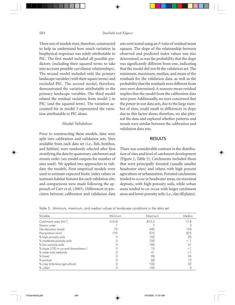
There was considerable contrast in the distribu-tion of sites and level of catchment development(Figure 1; Table 5). Catchments included thosethat were principally forested (usually smallerheadwater sites) and others with high percentagriculture or urbanization. Forested catchmentstended to occur in headwater areas, on morainaldeposits, with high-porosity soils, while urbanareas tended to co-occur with larger catchmentareas and lower porosity soils (i.e., clay till plains).

Table 5. Minimum, maximum, and median values of landscape conditions in the data set.

Variable Minimum Maximum Median

Catchment area (km2 ) 0.018 873.3 17.8Stream order 1 7 3Site elevation (masl) 75 440 176Precipitation (mm) 775 975 875% high porosity soils 0 100 25% moderate porosity soils 0 100 < 1% low porosity soils 0 100 61% slope (100 m up and downstream ) 0 10 <1% water and wetlands 0 41 <1% forest 0 98 24% pasture 0 68 12% crop (intensive agriculture) 0 100 52% urban 0 100 0

27stanfield2.p65 4/4/2006, 11:24 AM584


Fish Assemblages

We collected 64 fish species; 43 were present inless than 5% of the calibration sites. Of the re-maining species, eastern blacknose dace Rhini-chthys atratulus was found at 73% of all sites witha mean biomass of 67 g/100 m2 (Table 6). Scul-pins Cottus sp., creek chub Semotilus atroma-culatus, brook trout Salvelinus fontinalis, browntrout Salmo trutta, rainbow trout Oncorhynchusmykiss, and white sucker Catostomus commer-sonii were commonly occurring and abundant.Total fish biomass was 1.0–7,000 g/100 m2, and thenumber of fish species per site varied from 1 to 14.

The CCA illustrated four fish assemblage clus-ters (Figure 2). Axis 1 separated sites wheresalmonids were dominant from those with amore diverse mix of fishes where salmonids werea smaller component of the assemblage. Siteswith abundant salmonids tended to have higherforest cover and BFI ratings and lower PIC,whereas sites lacking salmonids tended to haveless forest cover, more urban area, lower BFI, andhigher PIC. The second CCA axis separated siteswith salmonid assemblages into those with brooktrout from those with other salmonid species.Brook trout tended to occur in sites with smallercatchments and greater elevations and slopes,while brown trout and rainbow trout tended to

occur in sites with larger catchments and lowerelevations and slopes. The second axis also sepa-rated sites with nonsalmonid taxa. Sites insmaller catchments supported species such asnorthern redbelly dace Phoxinus eos, fatheadminnow Pimephales notatus, and brook stickle-back Culaea inconstans, while darters Etheostomaspp. and rock bass Ambloplites rupestris weremore common in sites with larger catchments.

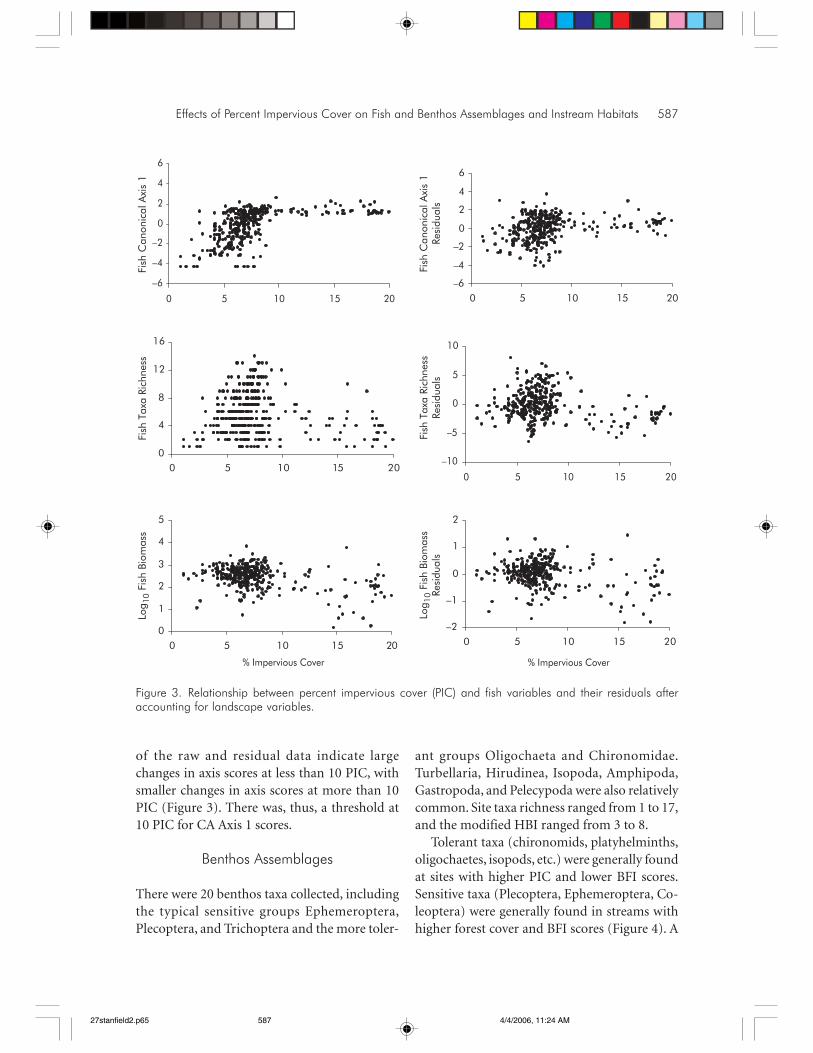
Percent impervious cover was a significantpredictor of each of the fish assemblage re-sponses, regardless of whether we modeled rawfish metrics or their residuals after accountingfor landscape features (Table 7). Relationshipsbetween PIC and fish assemblage metrics wereless apparent with residuals than with the origi-nal variables (Table 7; Figure 3) because PIC andBFI were related (Figure 2). Biomass weakly de-creased linearly with PIC (Figure 3). Species rich-ness was highest at more than 10 PIC, regardlessof whether the full or residual model was used(Figure 3). However, there was a weak bimodalpattern, where two sites with more than 15 PIChad species richness comparable to areas withless than 10 PIC. Scores of fish CA Axis 1 in-creased with PIC. The models for CA Axis 1 pre-dict the presence of salmonids in streams withlow PIC and an absence of salmonids in streamswith high PIC (Figure 2; Table 8). Scatterplots

Table 6. Distribution and biomass of common speciesa used in the model development.

Mean log biomass (g/100 m2)

% of sites with each taxa 0–0.5 0.5–1.0 1.0–1.5 1.5–2.0 2.0–2.5

5–10 BST CHS, FTD COS, LAM, NRD ROB10–20 RBD, PKS, BNM, CSH20–30 FHM BKT30–40 JOD BNT40–50 LND RBT50–60 SCU CRC, WS

60–70 BNDa BST = brook stickleback Culaea inconstans; CHS = Chinook salmon Oncorhynchus tshawytscha, FTD = fantail darter Etheostoma flabellare,COS = coho salmon O. kisutch, LAM = lamprey family Petromyzontidae, NRD = northern redbelly dace Phoxinus eos, ROB = rock bassAmbloplites rupestris, RBD = rainbow darter E. caeruleum), PKS = pumpkinseed Lepomis gibbosus, BNM = bluntnose minnow Pimephalesnotatus, CSH = common shiner Luxilus cornutus, FHM = fathead minnow P. promelas, BKT = brook trout Salvelinus fontinalis, JOD = Johnnydarter E. nigrum, BNT = brown trout Salmo trutta, LND = longnose dace Rhinichthys cataractae, RBT = rainbow trout O. mykiss, SCU =sculpin family Cottidae; CRC = creek chub Semotilus atromaculatus, WS = white sucker Catostomus commersonii, BND = eastern blacknosedace R. atratulus.

27stanfield2.p65 4/4/2006, 11:24 AM585


PIC

MinesWetland

Water

Fores tCrop

Pas ture Urban

BF I

BarrierLow P orMod Por

High P or P rec ipitation

Temperature

Elevation

S lope

S tr. Dis tanceOrderLink

S tr. LengthArea

SCU

JOD

FTD

RBD

PK S

ROB

BST

CRC

LND

BND

FHM

BNMCSH

NRD

WS

BKT

BNTRB T

CHSCOS

LA M

–1.5

-1

–0.5

0

0.5

1

1.5

–1.2 –1 –0.8 –0.6 –0.4 –0.2 0 0.2 0.4 0.6 0.8

CCA Axis 1

CC

A A

xis

2

Table 7. Regression models relating fish assemblage metrics to landscape and percent impervious cover (PIC)variables. There were three models for each response. Model 1 (the full model) relates the best landscape andPIC predictions to the response. Model 2 (reduced landscape model) relates the best landscape predictors (notincluding PIC) to the response. Model 3 relates the residuals from Model 2 to PIC.

Response variable

Log fish biomass Fish taxa richness Fish canonical axis 1

Model parameters 1 2 3 1 2 3 1 2 3

Constant –3.841 –5.075 0.129 –6.582 –3.741 –1.801 –1.625 2.465 –1.243Area 1.866 1.667Area2 –0.125 0.113 0.189 0.184Slope 0.125 –0.298 –0.243 –0.499Slope2 –0.017 0.027 0.052BFI 0.051 –0.016 –0.047BFI2 <–0.001 <0.001PIC –0.066 0.619 0.519 0.476 0.234PIC2 –0.002 –0.035 –0.031 –0.016 –0.008N 361 361 361 361 361 361 361 361 361MSE 0.215 0.242 0.218 5.895 6.380 5.835 0.804 0.949 0.870R2 0.185 0.085 0.087 0.372 0.319 0.085 0.394 0.280 0.081

Note: Each metric was squared to account for possible curvilinear relationships.

Figure 2. Relationship between landscape and fish assemblage composition as determined through canonicalcorrespondence analysis (CCA). Species acronyms are defined in Table 6. Por = porosity of soils; str = stream;PIC = percent impervious cover; BFI = baseflow index.

27stanfield2.p65 4/4/2006, 11:24 AM586


of the raw and residual data indicate largechanges in axis scores at less than 10 PIC, withsmaller changes in axis scores at more than 10PIC (Figure 3). There was, thus, a threshold at10 PIC for CA Axis 1 scores.

Benthos Assemblages

There were 20 benthos taxa collected, includingthe typical sensitive groups Ephemeroptera,Plecoptera, and Trichoptera and the more toler-

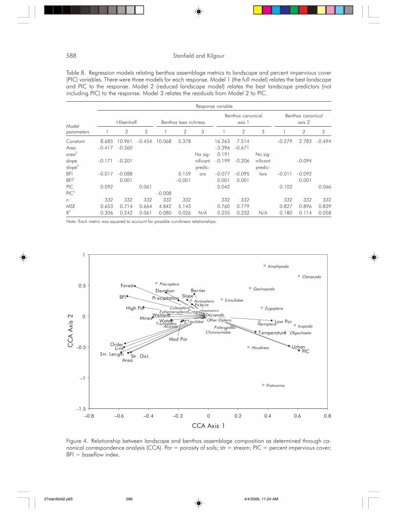
ant groups Oligochaeta and Chironomidae.Turbellaria, Hirudinea, Isopoda, Amphipoda,Gastropoda, and Pelecypoda were also relativelycommon. Site taxa richness ranged from 1 to 17,and the modified HBI ranged from 3 to 8.

Tolerant taxa (chironomids, platyhelminths,oligochaetes, isopods, etc.) were generally foundat sites with higher PIC and lower BFI scores.Sensitive taxa (Plecoptera, Ephemeroptera, Co-leoptera) were generally found in streams withhigher forest cover and BFI scores (Figure 4). A

–6

–4

–2

0

2

4

6

0 5 10 15 20

0

4

8

12

16

0 5 10 15 20–10

–5

0

5

10

0 5 10 15 20

0

1

2

3

4

5

0 5 10 15 20

–2

–1

0

1

2

0 5 10 15 20

–6

–4

–2

0

2

4

6

0 5 10 15 20

Log 1

0 Fi

sh B

iom

ass

Fish

Tax

a Ri

chne

ssFi

sh C

anon

ical

Axi

s 1

Log 1

0 Fi

sh B

iom

ass

Resi

dual

sFi

sh T

axa

Rich

ness

Re

sidu

als

Fish

Can

onic

al A

xis

1 Re

sidu

als

% Impervious Cover % Impervious Cover

Figure 3. Relationship between percent impervious cover (PIC) and fish variables and their residuals afteraccounting for landscape variables.

27stanfield2.p65 4/4/2006, 11:24 AM587


Table 8. Regression models relating benthos assemblage metrics to landscape and percent impervious cover(PIC) variables. There were three models for each response. Model 1 (the full model) relates the best landscapeand PIC to the response. Model 2 (reduced landscape model) relates the best landscape predictors (notincluding PIC) to the response. Model 3 relates the residuals from Model 2 to PIC.

Response variable

Benthos canonical Benthos canonical

ModelHilsenhoff Benthos taxa richness axis 1 axis 2

parameters 1 2 3 1 2 3 1 2 3 1 2 3

Constant 8.685 10.961 –0.454 10.068 5.378 16.263 7.514 –0.279 2.783 –0.494Area –0.417 –0.360 –3.396 –0.671area2 No sig- 0.191 No sig-slope –0.171 –0.201 nificant –0.199 –0.206 nificant –0.094slope2 predic- predic-BFI –0.017 –0.088 0.159 ors –0.077 –0.095 tors –0.011 –0.092BFI2 0.001 –0.001 0.001 0.001 0.001PIC 0.092 0.061 0.042 0.102 0.066PIC2 –0.008n 332 332 332 332 332 332 332 332 332 332MSE 0.653 0.714 0.664 4.842 5.143 0.760 0.779 0.827 0.896 0.839R2 0.306 0.242 0.061 0.080 0.026 N/A 0.255 0.232 N/A 0.180 0.114 0.058

Note: Each metric was squared to account for possible curvilinear relationships.

PIC

MinesWetland

Water

Forest

CropsPasture

Urban

BFIBarrier

Low Por

Mod Por

High Por

Pr ecipitation

Temperature

ElevationSlope

Str . Dist.

OrderLink

S tr. LengthArea

Other Diptera

Flatworms

IsopodaP elecypoda

Gastropoda

Trichoptera

Plecoptera

Anisoptera

ZygopteraMegaloptera

Hemiptera

EphemeropteraColeoptera

T ipulidae

S imuliidae

Chironomidae

Ostracoda

Decapoda

Amphipoda

Hirudinea

Oligochaeta

Acarina

–1.5

–1

–0.5

0

0.5

1

–0.8 –0.6 –0.4 –0.2 0 0.2 0.4 0.6 0.8

CCA Axis 1

CC

A A

xis

2

Figure 4. Relationship between landscape and benthos assemblage composition as determined through ca-nonical correspondence analysis (CCA). Por = porosity of soils; str = stream; PIC = percent impervious cover;BFI = baseflow index.

27stanfield2.p65 4/4/2006, 11:24 AM588


secondary environmental gradient was apparent inthe data, with amphipods, ostracods, and gastro-pods being more prevalent in smaller catchments.

As with fish assemblage metrics, indices ofbenthos assemblage composition were generallyrelated to PIC, even after accounting for the un-derlying influences of natural landscape features(Table 8). The HBI predictably increased withPIC, indicating degraded conditions. Values were4–5 for sites without development and averagedabout 6 for sites with full urbanization (i.e., 20%PIC). The HBI exhibited a weak threshold re-sponse at a 10 PIC (Figure 5). The relationshipbetween richness and PIC was statistically sig-nificant but not convincing. Benthos taxa rich-

ness was not significantly related to landscapefeatures other than BFI (Table 8). The benthosCA Axis 1 scores increased weakly with PIC (Fig-ure 5), but only for the full model (not the re-siduals), indicating that PIC may not beimportant for this metric. Correspondenceanalysis Axis 2 scores, however, did relate to PICafter removing the effects of natural landscapefactors and exhibited a weak threshold response(Figure 5). Correspondence analysis axis 2 scoresvaried between –2 and 3.5 at PIC less than 10,and there were no values greater than 0 abovePIC of 10. Sites with PIC greater than 10 con-tained higher proportions of mayflies, chirono-mids, isopods, and worms.

–4

–2

0

2

4

6

0 5 10 15 20

–6

–3

0

3

6

0 5 10 15 20

–4–3

–2–1

0

1234

0 5 10 15 20

–3

–2

–1

0

1

2

3

0 5 10 15 20

0

2

4

6

8

10

0 5 10 15 20

–4–3–2–1

01234

0 5 10 15 20

Hils

enho

ff sc

ore

Bent

hos

Can

onic

al A

xis

2Be

ntho

s C

anon

ical

Axi

s 1

Hils

enho

ff sc

ore

Resi

dual

sBe

ntho

s C

anon

ical

Axi

s 2

Resi

dual

sBe

ntho

s C

anon

ical

Axi

s 1

Resi

dual

s


Figure 5. Relationship between percent impervious cover (PIC) and benthos variables and their residuals afteraccounting for landscape variables.

27stanfield2.p65 4/4/2006, 11:24 AM589


Instream Habitat

The standardized stream temperature, propor-tion of stable banks, and mean width were re-lated to PIC, after the landscape conditions weretaken into consideration (Table 9). The otherphysical habitat and channel stability metricswere not related to PIC.

Standardized stream temperature and meanwidth were the only habitat attributes to dem-onstrate threshold-type responses to PIC, forboth the main and residual models, but thesewere weak relationships (Figure 6). There was amix of cold- and warmwater sites at less than 8PIC, and there were no coldwater sites above thisthreshold (Figure 6). Mean stream widths were0.5–20 m in catchments with PIC less than 10,but narrow streams were absent in catchmentswith higher PIC (Figure 6).

Model Validation

Fish CA axis 1, the modified HBI, standardizedtemperature, and the log of the width:depth ra-tio had the highest model fits with landscape data(Figure 7; Table 10). The slope of the predictedvalues for the validation and calibration data setsdiffered from unity for the fish CA axis 1 (Fig-ure 7). The validation data sets for all of the vari-ables, however, tended to produce scatterplotsthat were similar to the calibration scatterplots,suggesting that the models produced were rela-tively robust and that the data used to constructthe models were representative of the larger datasets. The lack of fit for the fish CA axis 1 is likelyrelated to either the extreme power in our dataor to other factors (not included in the model)also being important in explaining variation infish assemblages.

DISCUSSION

There are three principal conclusions from thisstudy. First, landscape measures accounted forsignificant variability in the responses of fish andbenthos assemblages, instream temperature, and

some instream habitat metrics. Second, PIC wasa significant modifier of the fish and benthosassemblage responses, as well as temperature,width:depth, and percent stable banks, even af-ter removing or accounting for the influences ofnatural landscape conditions. Third, fish andbenthos assemblages were clearly altered above10 PIC, and there were no coldwater streamsabove that threshold. Below the threshold, thebiophysical responses indicated that change inPIC would change fish, benthos, temperature,and the percent stable banks in an incrementalway. The landscape models developed here canbe used to predict fish and benthos assemblagesand habitat conditions, under a variety of land-use/land-cover scenarios, including an undis-turbed reference state. Each of these main pointsis discussed below.

Natural Landscape InfluenceBiophysical Responses

In this study, catchment area, slope, and the baseflow index were strong predictors of variation inindices of fish and benthos assemblages andstream temperature. These results were consis-tent with previous studies (e.g., Shaver andMaxted 1996; Richards et al. 1996, 1997; Kilgourand Barton 1999; Wang et al. 2001; Zorn et al.2002; Wang and Kanehl 2003). As has been ob-served previously (Horwitz 1978; Kilgour andBarton 1999; Zorn et al. 2002), we observed astrong gradient in the fish assemblages relatedto catchment size. Similar to Barton et al. (1985)for southwestern Ontario and Zorn et al. (2002)for lower Michigan, we found that brook troutwas generally limited to smaller catchments,while other salmonids were found in largercatchments. Stoneman and Jones (2000) provideevidence that this pattern of salmonid abun-dance is partly due to competition. It is also likelythat this relationship relates to the location ofsites relative to barriers in the catchment. TheCCA of the fish assemblage (Figure 2) indicateda weak tendency for brook trout to be moreprevalent upstream of barriers.

27stanfield2.p65 4/4/2006, 11:24 AM590


Tabl

e 9.

Regr

essi

on m

odel

s re

latin

g in

dice

s of

hab

itat

met

rics

to la

ndsc

ape

and

perc

ent

impe

rvio

us c

over

(PI

C)

varia

bles

. Th

ere

wer

e th

ree

mod

els

for

each

resp

onse

. Mod

el 1

(the

full

mod

el) r

elat

es th

e be

st la

ndsc

ape

and

PIC

to th

e re

spon

se. M

odel

2 (r

educ

ed la

ndsc

ape

mod

el) r

elat

es th

e be

st la

ndsc

ape

pred

icto

rs(n

ot in

clud

ing

PIC

) to

the

resp

onse

. Mod

el 3

rel

ates

the

resi

dual

s fro

m M

odel

2 to

PIC

.

Resp

onse

var

iabl

e

Mod

el S

tream

tem

pera

ture

Mea

n w

idth

:dep

thPr

opor

tion

stab

le b

anks

Cha

nnel

sta

bilit

yM

ean

stre

am w

idth

para

met

ers

12

31

23

12

31

23

12

3

cons

tant

12.5

21.3

82–2

.683

0.72

70.

962

–0.0

270.

992

1.16

7–0

.052

2.22

9–0

.455

–0.2

560.

123

area

0.98

9–0

.003

–0.0

30–0

.571

0.03

1ar

ea2

0.07

30.

018

0.01

70.

046

0.03

0slo

pe–1

.818

–2.1

040.

082

0.02

7–0

.012

–0.0

380.

034

–0.0

66sl

ope2

0.18

30.

206

–0.0

090.

004

BFI

–0.0

19–0

.023

–0.0

28–0

.035

BFI2

–0.0

01–0

.001

0.00

020.

0002

–0.0

001

<0.

001

<0.

001

PIC

0.89

10.

560

0.02

20.

011

–0.0

36PI

C2

–0.0

34–0

.022

0.00

050.

0004

–0.0

008

–0.0

004

0.00

10.

002

n38

538

538

537

037

037

035

335

335

335

337

337

337

3M

SE10

.310

.611

10.3

130.

039

0.04

00.

039

0.00

80.

008

0.00

80.

044

NA

NA

0.49

10.

051

0.04

8R2

0.27

80.

263

0.02

30.

357

0.33

20.

022

0.08

20.

077

0.01

00.

069

0.60

70.

590

0.04

8

Resp

onse

var

iabl

e

Mod

elD

50po

int

D50

max

Sorti

ng in

dex

Hom

ogen

eity

para

met

ers

12

31

23

12

31

23

Con

stan

t–1

.313

–1.1

30–2

.493

–2.1

800.

635

2.05

2Ar

eaAr

ea2

0.04

00.

040

0.06

70.

066

–0.0

23Sl

ope

0.40

10.

406

0.67

40.

618

–0.1

28Sl

ope2

–0.0

29–0

.029

–0.0

56–0

.048

BFI

–0.0

100.

049

BFI2

–0.0

001

–0.0

002

–0.0

006

0.00

01PI

C–0

.000

1PI

C2

0.00

2N

369

363

363

363

MSE

0.34

5N

AN

A1.

0254

1.03

7N

A0.

061

NA

NA

0.86

6N

AN

AR2

0.23

70.

224

0.21

30.

032

0.05

3

Not

e: E

ach

met

ric w

as s

quar

ed to

acc

ount

for

poss

ible

cur

vilin

ear

rela

tions

hips

. NA

indi

cate

s no

sig

nific

ant m

odel

det

erm

ined

.

27stanfield2.p65 4/4/2006, 11:24 AM591


In catchments with poorly drained soils, as-sociations between catchment area and the fishfauna were not surprising. Brook stickleback,northern redbelly dace, and fathead minnowwere more common in streams draining smallercatchments, while rock bass, rainbow darterEtheostoma caeruleum, and longnose daceRhinichthys cataractae were more common instreams draining larger catchments. These asso-ciations were subtle, but have been reported be-fore for southern Ontario (Kilgour and Barton1999) and agree for the most part with findingsfrom lower Michigan (Zorn et al. 2002). In lowerMichigan, brook stickleback and northern red-belly dace were found in larger catchments thanin our study and the difference in catchment sizebetween where rock bass and rainbow darterswere found was less distinct than what we ob-served. These differences are likely due to themuch larger catchment size range in the Michi-gan study (i.e., maximum catchment sizes ex-ceeded 10,000 km2 compared to 873 km2 in ourstudy).

In this study, salmonids were generally foundat sites with higher slopes. The influence of slopehas been demonstrated in several other studiesbut notably by Wang and Kanehl (2003). Streamswith greater slopes offer higher energy regimes(Rosgen 1996), higher groundwater contribu-tions (Baker et al. 2001), and potential refuge forbrook trout from migratory salmonid competi-tors. Catchments with higher gradients producegreater head for groundwater movement andstreams with higher gradients tend to cut deeperinto alluvial materials increasing the potential tointersect the water table.

The importance of surficial geology as a pri-mary influence on fish and benthos assemblageswas reconfirmed in this study. Many other stud-ies have demonstrated the significance of surficialgeology, notably Portt et al. (1989) for southernOntario streams. In this study, we used an indexof base flow to capture the surficial geology influ-ence and found it highly predictive of fish andbenthos assemblages. Though our index of baseflow potential differed from others (e.g., Zorn et

0

10

20

30

40

0 5 10 15 20

–10–8–6–4–202468

10

0 5 10 15 2

–0.4

–0.2

0

0.2

0.4

0 5 10 150

0.5

1

1.5

2

0 5 10 15 20

Log 1

0 W

idth

Std.

Tem

pera

ture

Log 1

0 W

idth

Res

idua

lsSt

d. T

empe

ratu

re R

esid

uals


Figure 6. Relationship between percent impervious cover (PIC) and standardized temperature and mean widthand their residuals after accounting for landscape variables.

27stanfield2.p65 4/4/2006, 11:24 AM592


al. 2002; Wang et al. 2003), the results were simi-lar in that coldwater species were more frequentlyobserved in streams with high base flow potential(i.e., were draining areas of high porosity glacialmaterials). Although our models explained rela-tively little variation in the response variables, themodels were apparently robust and reflected whatis intuitively known about the relationships be-tween stream biophysical responses and landscapeattributes. There should, therefore, be reasonable

confidence in using the derived models for un-derstanding the relationships between stream bio-physical responses and landscape and land-use/land-cover conditions.

PIC Effects

Even after considering the effects of natural land-scape variables (i.e., size, surficial geology/baseflow and slope), there were significant variations

2 3 4 5 6 7 8 9

Predicted

2

3

4

5

6

7

8

9

0.5 1.0 1.5 2.0 2.50.5

1.0

1.5

2.0

2.5

10 15 20 25 30 3510

15

20

25

30

35TemperatureLog Width:Depth

Hilsenhoff

–3 –2 –1 0 1 2

Predicted

–3

–2

–1

0

1

2

3CA Axis 1: Fish

Obs

erve

dO

bser

ved

Obs

erve

dO

bser

ved

Predicted Predicted

Figure 7. Relationship between observed and predicted biophysical indices illustrating the general fit of thebest-fitting models. Filled circles are calibration data, open circles are validation data. The solid line is the 1:1line of expectation (calibration data), while the dotted line is for the validation data.

27stanfield2.p65 4/4/2006, 11:24 AM593


in biophysical responses related to PIC. Metricsof fish assemblages and temperature varied withPIC between background conditions (~0–3) tohighly urbanized (>10) (Figures 3 and 6). Be-low 10 PIC, there was considerable noise in thebiological metrics, reflecting influences of otherlandscape variables (i.e., base flow, catchmentsize, slope) and local modifying factors such asriparian zones (Barton et al. 1985), adjacent landuse, and instream habitat complexity. The ob-served relationships, however, indicate that in-crease in PIC will result in changes (i.e.,degradation) in biological assemblages. Thesedata also suggest that locally applied best-man-agement practices and restoration activities arelikely to be most effective when applied tostreams with less than 10 PIC. Wang et al. (2006,this volume) reached a similar conclusion forWisconsin and Michigan streams.

It was surprising that few geomorphic metricswere associated with PIC (Table 9). The mea-sures used have been demonstrated to be pre-cise (Stanfield and Jones 1998); therefore, the lackof association is unlikely related to measurementerror. We also know that geomorphic attributesof streams respond to changes in PIC in thecatchment (Leopold 1968) and that hydrologicfactors are important in determining the kindsof fish and invertebrates found in streams (Zornet al. 2002). The geomorphic variables that didvary in relation to landscape variables (includ-

ing PIC) included width:depth ratio, which is aclassic indicator of an urbanized stream (i.e.,wider and shallower in urban areas), and per-cent stable banks. The other geomorphic vari-ables (stability, D50point, D50max, sorting index,and homogeneity) are essentially measures ofsubstrate. That these factors did not relate wellto landscape features indicates that they may bemore controlled by local factors, such as sinuos-ity, gradient and riparian conditions (Rosgen1996), and potentially local soil types.

An alternative hypothesis is that our data setincluded an insufficient number of sites exhib-iting stable geomorphic conditions. Several stud-ies suggest that channel stability is even moresensitive to PIC than biological variables (Dunneand Leopold 1978; Booth and Jackson 1997).Further, geomorphic processes require hundredsto thousands of years to reestablish equilibrium.The study area was deforested in the 1800s andsustained serious instream modifications untilreforestation and soil protection began in the1930s (Richardson 1944). Stream morphologyand stability in this study area likely reflect thehistoric changes in the landscape and recent de-velopment patterns (i.e., urban sprawl). Ourfindings suggest that more effort is required tosort historic from current impacts on channelgeomorphology and to assess the value of thesegeomorphic metrics as indicators of overallstream condition.

Table 10. Validation of the best-fitting biophysical models. Differences in precision between calibration andvalidation data sets was tested using an F-ratio of residual mean squares. The slope of the relationship be-tween observed and predicted index values was also determined, as was the probability that the slope was one,indicating that the model fit the validation set. The minimum, maximum, median, and mean of the residuals forthe validation data and the probability that the residuals were zero are also provided. A non-zero meanresidual implies a bias in the validation data.

Precision Observed vs. predicted Residual statistics

Model Fval/cal Pval = cal Slope (SE) Pslope = 1 Mean Pmean = 0

Fish canonical axis 1 1.032 0.384 0.714 (0.078) 0.0003 –0.009 0.852Hilsenhoff biotic index 1.230 0.044 0.973 (0.112) 0.807 –0.064 0.284Stream temperature 1.054 0.328 0.921 (0.115) 0.492 0.118 0.588Log10width:depth 1.301 0.017 1.199 (0.117) 0.090 0.017 0.282

27stanfield2.p65 4/4/2006, 11:24 AM594


The PIC Threshold

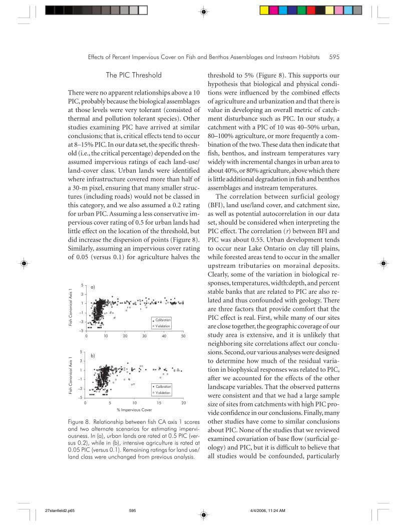
There were no apparent relationships above a 10PIC, probably because the biological assemblagesat those levels were very tolerant (consisted ofthermal and pollution tolerant species). Otherstudies examining PIC have arrived at similarconclusions; that is, critical effects tend to occurat 8–15% PIC. In our data set, the specific thresh-old (i.e., the critical percentage) depended on theassumed impervious ratings of each land-use/land-cover class. Urban lands were identifiedwhere infrastructure covered more than half ofa 30-m pixel, ensuring that many smaller struc-tures (including roads) would not be classed inthis category, and we also assumed a 0.2 ratingfor urban PIC. Assuming a less conservative im-pervious cover rating of 0.5 for urban lands hadlittle effect on the location of the threshold, butdid increase the dispersion of points (Figure 8).Similarly, assuming an impervious cover ratingof 0.05 (versus 0.1) for agriculture halves the

threshold to 5% (Figure 8). This supports ourhypothesis that biological and physical condi-tions were influenced by the combined effectsof agriculture and urbanization and that there isvalue in developing an overall metric of catch-ment disturbance such as PIC. In our study, acatchment with a PIC of 10 was 40–50% urban,80–100% agriculture, or more frequently a com-bination of the two. These data then indicate thatfish, benthos, and instream temperatures varywidely with incremental changes in urban area toabout 40%, or 80% agriculture, above which thereis little additional degradation in fish and benthosassemblages and instream temperatures.

The correlation between surficial geology(BFI), land use/land cover, and catchment size,as well as potential autocorrelation in our dataset, should be considered when interpreting thePIC effect. The correlation (r) between BFI andPIC was about 0.55. Urban development tendsto occur near Lake Ontario on clay till plains,while forested areas tend to occur in the smallerupstream tributaries on morainal deposits.Clearly, some of the variation in biological re-sponses, temperatures, width:depth, and percentstable banks that are related to PIC are also re-lated and thus confounded with geology. Thereare three factors that provide comfort that thePIC effect is real. First, while many of our sitesare close together, the geographic coverage of ourstudy area is extensive, and it is unlikely thatneighboring site correlations affect our conclu-sions. Second, our various analyses were designedto determine how much of the residual varia-tion in biophysical responses was related to PIC,after we accounted for the effects of the otherlandscape variables. That the observed patternswere consistent and that we had a large samplesize of sites from catchments with high PIC pro-vide confidence in our conclusions. Finally, manyother studies have come to similar conclusionsabout PIC. None of the studies that we reviewedexamined covariation of base flow (surficial ge-ology) and PIC, but it is difficult to believe thatall studies would be confounded, particularly

–5

–3

–1

1

3

5

0 10 20 30 40 50

Calibration

Validation

–5

–3

–1

1

3

5

0 5 10 15 20

Calibration

Validation

a)

b)

% Impervious Cover

Fish

Can

onic

al A

xis

1Fi

sh C

anon

ical

Axi

s 1

Figure 8. Relationship between fish CA axis 1 scoresand two alternate scenarios for estimating impervi-ousness. In (a), urban lands are rated at 0.5 PIC (ver-sus 0.2), while in (b), intensive agriculture is rated at0.05 PIC (versus 0.1). Remaining ratings for land use/land class were unchanged from previous analysis.

27stanfield2.p65 4/4/2006, 11:24 AM595


those studies conducted in places like Delawarethat have not experienced glaciations. Regard-less, our understanding of the PIC effect insouthern Ontario would benefit from additionaldata from sites on morainal deposits, with higherlevels of PIC.

Use of Models for Hindcasting

Our models illustrate the magnitude and natureof relationships between biophysical responsesand landscape features (natural and anthropo-genic), and they can be used for two contrastingbut interrelated purposes: hindcasting expectedreference conditions and predicting future con-ditions assuming development scenarios. Theability to hindcast allows one to predict the bio-physical makeup of a stream in the absence ofdevelopment. The reference-condition approach(Hughes 1994; Bailey et al. 1998), in which re-gional reference sites are used to characterizeacceptable biological conditions, requires least orminimally disturbed reference sites. In southernOntario, there are no unaltered catchments. De-fining reference condition, therefore, is biasedtoward disturbance and the definition mighthave to change with catchment size because thereare no large catchments lacking development.Our models, however, have taken catchment sizeand other variables into consideration. They cantherefore be used to estimate what conditionsmight have been in the absence of development.Current and future conditions can then be com-pared to the predicted historical condition, toestimate the magnitude and nature of change incondition. One limitation to the models is thatthey should not be used to hindcast to condi-tions that did not exist as part of the calibrationdata set. Thus, the hindcast reference conditionfor large catchments might not be 100% forestcover. Kilgour and Stanfield (2006, this volume)are using this approach to compare current con-ditions with hindcast historical conditions in theLake Ontario study area as a means of charac-terizing the state of the ecosystem.

Other Considerations

We developed models for a few fish, benthos andinstream habitat metrics, which likely differ fromthose others might have chosen. The methodswe selected provide both an overview of basicfeatures of assemblages (i.e., biomass for fish andnumber of taxa for fish and benthos), as well asaxis scores from correspondence analysis. As aresult, we are confident that the models producedhere are robust and that it would be unlikely thata different conclusion would be reached with adifferent set of variables. Given that the resultsobtained for fish and benthos in southernOntario are similar to results obtained for otherparts of North America, we are confident thatthe patterns identified in this data set are robust.

Finally, this study employed fairly coarse mea-sures of land use/land cover and no analysis ofproximity effects (i.e., the degree to which fea-tures closer to a site influenced its condition).Future efforts will be directed at refining the re-lationships shown here, using finer measures ofland use/land cover and proximity effects and toidentifying those additional variables that con-tribute to explained variability in fish assem-blages. In addition, we intend to explore thedegree to which riparian best management prac-tices and instream habitat complexity buffer theeffects of PIC.

ACKNOWLEDGMENTS

Mike Stoneman developed the database and dataqueries. Randal Kuyvenhoven and Frank Kennydeveloped the GIS applications for extractingland-use/land-cover information. Brent Harlowassisted with data compilation and ran the GISapplication. Colleen Lavender validated the lo-cation of each site on the landscape. Laurie Allin,Jeff Anderson, Jon Clayton, Marc Desjardins,Scott Jarvie, and Bernie McIntyre assisted withdata collection and conceptual discussions.Helen Ball, Jason Borwick, Scott Gibson, SteveHolysh, Don Jackson, Chris Jones, Rob

27stanfield2.p65 4/4/2006, 11:24 AM596


McLaughlin, Nick Mandrak, Mark Peacock, TimRance, Keith Somers, and Chris Wilson providedadvice on the approach and data analysis tech-niques. Gen Carr assisted with data analysis andKeith Somers reviewed the analysis. Cheryl Lewisensured support for the project. Bob Hughes, AlCurry, and one anonymous reviewer providedvaluable comments on an earlier draft. Ottawa,Toronto, Environment Canada, Michigan De-partment of Natural Resources and the OntarioMinistry of Natural Resources provided fund-ing at various stages.

REFERENCES

Arnold, C. L., and C. J. Gibbons. 1996. Impervious

surface coverage: the emergence of a key environ-

mental indicator. Journal of American Planning

62:243–258.

Bailey, R. C., M. G. Kennedy, M. Z. Dervish, and R. M.

Taylor. 1998. Biological assessment of freshwater

ecosystems using a reference condition approach:

comparing predicted and actual benthos inverte-

brate communities in Yukon streams. Freshwater

Biology 39:765–774.

Baker, M. E., M. J. Wiley, and P. W. Seelbach. 2001. GIS-

based hydrologic models of riparian areas: implica-

tions of stream water quality. Journal of the American

Water Resources Association 37:1615–1628.

Barton, D. R., W. D. Taylor, and R. M. Biette. 1985.

Dimensions of riparian buffer strips required to

maintain trout habitat in southern Ontario

streams. North American Journal of Fisheries Man-

agement 5:364–378.

Booth, D. B., and C. R. Jackson. 1997. Urbanization of

aquatic systems: degradation thresholds,

stormwater detection, and the limits of mitigation.

Journal of the American Water Resources Associa-

tion 33:1077–1090.

Carr, G. M., S. A. E. Bod, H. C. Duthie, and W. D. Tay-

lor. 2003. Macrophyte biomass and water quality

in Ontario rivers. Journal of the North American

Benthological Society 22:182–193.

Dunne, T., and L. B. Leopold. 1978. Water in environ-

mental planning. Freeman, New York.

Gauch, H. G. 1982. Multivariate analysis in commu-

nity ecology. Cambridge University Press, Cam-

bridge, England

Harding, J. S., R. G. Young, J. W. Hayes, K. A. Shearer,

and J. D. Stark. 1999. Changes in agricultural in-

tensity and river health along a river continuum.

Freshwater Biology 42:345–357.

Hilsenhoff, W. L. 1987. An improved biotic index of

organic stream pollution. Great Lakes Entomolo-

gist 20:31–39.

Horwitz, R. J. 1978. Temporal variability patterns and

the distribution patterns of streams fishes. Ecologi-

cal Monographs 48:307–321.

Hughes, R. M. 1994. Defining acceptable biological

status by comparing with reference conditions.

Pages 31–47 in W. S. Davis and T. P. Simon, edi-

tors. Biological assessment and criteria: tools for

water resource planning and decision making.

Lewis, Boca Raton, Florida.

Jones, J. B., and C. C. Clark. 1987. Impact of water-

shed urbanization on stream insect communities.

Water Resources Bulletin 23:1047–1055.

Jones, M. L., and J. D. Stockwell. 1995. A rapid assess-

ment procedure for enumeration of salmonine

populations in streams. North American Journal

of Fisheries Management 15:551–562.

Kilgour, B. W., and D. R. Barton. 1999. Associations

between stream fish and benthos across environ-

mental gradients in southern Ontario, Canada.

Freshwater Biology 41:553–566.

Kilgour, B. W., and L. W. Stanfield. 2006. Hindcasting

reference conditions in streams. Pages 623–639 in

R. M. Hughes, L. Wang, and P. W. Seelbach, edi-

tors. Landscape influences on stream habitats and

biological assemblages. American Fisheries Soci-

ety, Symposium 48, Bethesda, Maryland.

Klein, R. D. 1979. Urbanization and stream quality

impairment. Water Resources Bulletin 15:948–963.

Leopold, L. B. 1968. Hydrology for urban land plan-

ning: a guidebook on the hydrologic effects of ur-

ban land use. Geological Survey Circular 554,

Washington, D.C.

Limburg, K. E., and R. E. Schmidt. 1990. Patterns of

fish spawning in Hudson River tributaries: response

to an urban gradient? Ecology 71:1238–1245.

27stanfield2.p65 4/4/2006, 11:24 AM597


Lyons, J. 1992. The length of stream to sample with a

towed electrofishing unit when fish species rich-

ness is estimated. North American Journal of Fish-

eries Management 12:198–203.

May, W. M., R. R. Horner, J. R. Karr, B. W. Mar, and E.

B. Welch. 1997. Effects of urbanization on small

streams in the Puget Sound Lowland ecoregion.

Watershed Protection and Technology 2:483–494.

Ontario Geological Survey. 1997. Quaternary geology,

seamless coverage of the province of Ontario,

ERLIS data set 14. Ontario Ministry of Northern

Development and Mines, Sudbury.

Piggott, A., D. Brown, and S. Moin. 2002. Calculating a

groundwater legend for existing geological mapping

data. Environment Canada, Burlington, Ontario.

Plafkin, J. L., M. T. Barbour, K. D. Porter, S. K. Gross,

and R. M. Hughes. 1989. Rapid bioassessment pro-

tocols for use in streams and rivers: benthic

macroinvertebrates and fish. U.S. Environmental

Protection Agency, EPA/440/4–89/001, Washing-

ton, D.C.

Portt, C. B., S. W. King, and H. B. N. Hynes. 1989. A

review and evaluation of stream habitat classifica-

tion systems with recommendations for the devel-

opment of a system for use in southern Ontario.

Ontario Ministry of Natural Resources, Toronto.

Prisloe, S., Y. Lei, and J. Hurd. 2001. Interactive GIS-

based impervious surface model. American Soci-

ety of Photogrammetry and Remote Sensing,

Bethesda, Maryland.

Richards C, R. J. Haro, L. B. Johnson, and G. E. Host.

1996. Landscape scale influences on stream habi-

tat and biota. Canadian Journal of Fisheries and

Aquatic Sciences 53(supplement 1):295–311.

Richards, C., R. J. Haro, L. B. Johnson, and G. E. Host.

1997. Catchment and reach-scale properties as in-

dicators of macroinvertebrate species traits. Fresh-

water Biology 37:219–230.

Richardson, A. H. 1944. A report on the Ganaraska

watershed: a study in land use with plans for the

rehabilitation of the area in the post-war period.

Ontario Department of Planning and Develop-

ment, Toronto.

Rosgen, D. L. 1996. Applied river morphology. Wild-

land Hydrology, Pagosa Springs, Colorado.

Shaver, E. J., and J. R. Maxted. 1995. The use of imper-

vious cover to predict ecological condition of wade-

able nontidal streams in Delaware. Delaware County

Planning Department, Ellicott City, Maryland.

Shaver, E. J., and J. R. Maxted. 1996. Habitat and bio-

logical monitoring reveals headwater stream im-

pairment in Delaware’s piedmont. Watershed

Protection Techniques 2(2):358–360.

Stanfield, L. W., M. Jones, M. Stoneman, B. Kilgour, J.

Parish, G. Wichert. 1997. Stream assessment pro-

tocol for Ontario. Ontario Ministry of Natural

Resources, Glenora.

Stanfield, L. W., and M. L. Jones. 1998. A comparison

of full-station visual and transect-based methods

of conducting habitat surveys in support of habi-

tat suitability index models for southern Ontario.

North American Journal of Fisheries Management

18:657–675.

Stanfield, L. W., and R. Kuyvenhoven. 2003. Protocol

for applications used in the aquatic landscape in-

ventory software application: a tool for delineat-

ing, characterizing and classifying valley segments

within the Great Lakes basin. Ontario Ministry of

Natural Resources, Peterborough.

Statistics Canada. 2003. Statistics Canada population

estimates and Ministry of Finance population pro-

jections, 1999–2028. Cabinet Office of the Prov-

ince of Ontario, Toronto.

Steedman, R. J. 1988. Modification and assessment of

an index of biotic integrity to quantify stream qual-

ity in southern Ontario. Canadian Journal of Fish-

eries and Aquatic Sciences 45:492–501.

Stoneman, C. L., and M. L. Jones. 2000. The influence

of habitat features on the biomass and distribu-

tion of three species of southern Ontario stream

salmonines. Transactions of the American Fisher-

ies Society 129:639–657.

Stoneman, C. L., and M. L. Jones. 1996. A simple meth-

odology to evaluate the thermal stability of trout

streams. North American Journal of Fisheries Man-

agement 16:728–737.

ter Braak, C. J. F. 1992. CANOCO—a FORTRAN pro-

gram for canonical assemblage ordination. Micro-

computer Power, Ithaca, New York.

Wang, L., J. Lyons, P. Kanehl, R. Bannerman, and E.

27stanfield2.p65 4/4/2006, 11:24 AM598


Emmons. 2000. Watershed urbanization and

changes in fish communities in southeastern Wis-

consin streams. Journal of the American Water

Resources Association 36:1173–1189.

Wang, L., J. Lyons, P. Kanehl, and R. Bannerman. 2001.

Impacts of urbanization on stream habitat and fish

across multiple spatial scales. Environmental Man-

agement 28:255–266.

Wang, L., and P. Kanehl. 2003. Influences of water-

shed urbanization and in-stream habitat on

macroinvertebrates in cold water streams. Journal

of the American Water Resources Association

39:1181–1196.

Wang, L., J. Lyons, P. Rasmussen, P. Seelbach, T.

Simon, M. Wiley, P. Kanehl, E. Baker S. Niemela,

and P. M. Stewart. 2003. Watershed, reach and ri-

parian influences on stream fish assemblages in

the Northern Lakes and Forest ecoregion, U.S.A.

Canadian Journal of Fisheries and Aquatic Sci-

ences 60:491–505.

Wang, L., P. W. Seelbach, and J. Lyons. 2006. Effects of

levels of human disturbances on the influence of

catchment, riparian, and reach-scale factors on fish

assemblages. Pages 199–219 in R. M. Hughes, L.

Wang, and P. W. Seelbach, editors. Landscape in-

fluences on stream habitats and biological assem-

blages. American Fisheries Society, Symposium 48,

Bethesda, Maryland.

Yoder, C .O., R. J. Miltner, and D. White. 1999. Assess-

ing the status of aquatic life designated uses in ur-

ban and suburban watersheds. Pages 16–28 in

Proceedings of the national conference on retrofit

opportunities for water resource protection in ur-

ban environments. U.S. Environmental Protection

Agency, Washington, D.C.

Zorn T. G., P. W. Seelbach, and M. J. Wiley. 2002. Dis-

tributions of stream fishes and their relationship

to stream size and hydrology in Michigan’s lower

peninsula. Transactions of the American Fisheries

Society 131:70–85.

27stanfield2.p65 4/4/2006, 11:24 AM599

27stanfield2.p65 4/4/2006, 11:24 AM600

effects of percent impervious cover on fish and benthos ... · effects of percent impervious cover...

Documents