effects of income inequality on china’s economic growth

Journal of Policy Modeling 31 (2009) 69–86

Available online at www.sciencedirect.com

Effects of income inequality onChina’s economic growth�

Duo Qin a,∗, Marie Anne Cagas c, Geoffrey Ducanes d,Xinhua He b, Rui Liu b, Shiguo Liu b

a Queen Mary, University of London, Mile End Road, London E1 4NS, UKb Institute of World Economics & Politics (IWEP), Chinese Academy of Social Sciences (CASS), China

c SAS Institute, Philippinesd University of the Philippines, Philippines

Received 1 February 2008; received in revised form 1 June 2008; accepted 1 August 2008Available online 19 September 2008

Abstract

A pilot empirical study is carried out on how income inequality affects growth through incorporatingpanel data information into a quarterly macro-econometric model of China. Provincial urban and ruralhousehold data are used to construct income inequality measures, which are then used to augment householdconsumption equations in the model. Model simulations test the inequality effect on GDP growth and itscomponents. Results show that income inequality forms robust explanatory variables of consumption andthat the way inequality develops carries negative consequences on GDP and sectoral growth.© 2008 Society for Policy Modeling. Published by Elsevier Inc. All rights reserved.

JEL classification: R11; E21; D3; C5; C2

Keywords: Income inequality; Growth; Macroeconometric model; China

1. Introduction

Since undertaking market reforms, the Chinese economy has achieved sustained high growthand rapid progress in poverty reduction. The World Bank estimates that in the more than two

� This study was carried out when the authors were working together on a macroeconometric modeling project forAsian Development Bank.

∗ Corresponding author at: Department of Economics, Queen Mary, University of London, Mile End Road, London E14NS, UK. Tel.: +44 2078823641.

E-mail address: [email protected] (D. Qin).

0161-8938/$ – see front matter © 2008 Society for Policy Modeling. Published by Elsevier Inc. All rights reserved.doi:10.1016/j.jpolmod.2008.08.003

mailto:[email protected]

dx.doi.org/10.1016/j.jpolmod.2008.08.003

70 D. Qin et al. / Journal of Policy Modeling 31 (2009) 69–86

decades since reforms started, average income per capita in China has quadrupled while morethan 270 million people have been lifted out of poverty (Chen & Wang, 2001). GDP growth inChina averaged nearly 10% annually for the past decade, and it has not yet shown signs of slowingdown.

If there seems to be a dark lining to these extraordinary achievements, it is that income inequalityin the country – seen as a whole, within/between urban and rural areas, and across provinces – hasalso risen quite rapidly in the period (see, for example, Chen & Wang, 2001; Zhang & Kanbur,2005; World Bank, 1997). Income inequality is generally seen to affect long-term economicgrowth, although there is no consensus on the direction of the effect. If income inequality affectsgrowth positively, it is possible that the poverty-reducing impact of this growth offsets the directadverse effect of inequality on welfare, and thus reason to tolerate relatively high inequality. Onthe other hand, if inequality affects growth negatively, then addressing it immediately should bean important concern.

This paper investigates empirically how much and in what ways income inequality affectsChina’s economic growth by means of incorporating income disparity measures derived fromprovincial panel data of urban and rural household income into a macro-econometric model, andsimulating the effects of changes in income inequality on growth. The rest of the paper is structuredas follows. Section 2 gives a summary of the inequality situation in China. Section 3 briefly surveysthe literature on the transmission mechanism between income inequality and economic growth.Section 4 describes our modeling approach and discusses available inequality measures whichmight be pertinent to our investigation. Section 5 describes the estimation results of incorporatingincome inequality into the macro-econometric model. Section 6 presents the results of modelsimulations showing the effects of inequality changes on other economic variables. The last sectionconcludes with a summary of the findings and a brief discussion of relevant policy implications.

2. Background on income inequality in China

Income inequality had remained fairly mild and stable under an egalitarian regime prior tothe economic reform, which started in 1978. According to Li, Zhang, Wei, and Zhong (2000, pp.3–4), the Gini ratio of urban households was 0.16, the Gini ratio for rural households was 0.21in 1978,1 and the Gini ratio among the provinces was 0.14 in 1979. The situation has changedconsiderably since the reform. According to a World Bank report (1997), China has undergonethree different periods since 1980 as far as the growth-equity characteristics are concerned. Theperiod 1981–1984 is classified as one of growth with equity, during which real mean incomeincreased by 12.6% annually while the Gini ratio rose only marginally. The period 1984–1989 isclassified as one of income inequality with little growth, during which overall real mean incomeincreased by less than 1% annually while the growth was very unevenly distributed.2 The thirdperiod from 1990 onwards is one of growth with income inequality as both overall real meanincome and the Gini ratio grew rapidly.

The aggregate Gini ratios have been estimated in several studies. Krongkaew (2003) reportsthe per capita income Gini ratio to be 0.29 in 1981, and to have risen to 0.30 in 1984, 0.35 in1989, 0.39 in 1995, and 0.46 in 2000. Li et al. (2000, p. 8) estimate that within rural areas the

1 Li et al. (2000, p. 3) list several estimates for rural households’ Gini ratio: 0.21 estimated by the Chinese NationalBureau of Statistics in 1978, 0.22 estimated by Adelman and Sunding in 1987, and 0.31 estimated by the World Bank in1983.

2 However, this description may not be so accurate if we look at the official statistics on per capita GDP.

D. Qin et al. / Journal of Policy Modeling 31 (2009) 69–86 71

Fig. 1. Per capita household income (RMB per quarter).

Gini ratio of household income rose from 0.21 to 0.34 for the period 1979–1995 and that withinurban areas the Gini ratio went up from 0.16 to 0.28 in the same period. Li et al. (2000) andZhang (2003), meanwhile, report the inter-provincial per capita income Gini ratio to have beenrising almost consistently from 0.32 in 1978, to 0.28 in 1983, 0.38 in 1988, 0.39 in 1995, 0.40 in1999, and 0.42 in 2000.

However, the most striking feature of the rising inequality is probably the increasing incomegap between the rural and urban sectors. Some researchers have claimed it to be the world’s largest(e.g. see Lin, 2003). Inequality decompositions done by the government show that the rural–urbanincome gap explained one-third of total inequality in 1995 and one-half the increase in inequalitysince 1985. Rural per capita income was 38.9% of urban per capita income in 1978, 53.8% in1985, and was down to 35.9% in 2000 (Lin, 2003). Li et al. (2000) note the same diverging path ofrural and urban incomes. This does not even take into account the set of publicly provided services– housing, pensions, health, education, and other entitlements – that augment urban incomes byan average of 80%. When these are considered, rural–urban disparities accounted for an evengreater share of total inequality (World Bank, 1997). Fig. 1 shows for the period 1992–2003 thewidening gap between urban and rural per capita incomes.

Income inequality has also risen geographically, the most pronounced being between coastaland interior provinces. Inter-provincial inequality accounted for a quarter of total inequality in1995 and explained a third of the increase since 1985. In 1985, residents of interior China earned75% as much as their coastal counterparts, by 1995 this had dropped to 50% (World Bank, 1997).

3. Inequality → growth nexus: background literature

A famous postulate on income inequality and growth was put forward by Kuznets (1955). Thepostulate says that in the course of a country’s development, inequality first rises before eventuallydeclining—the inverted-U hypothesis. However, Kuznet’s hypothesis implies a causal relationshipof growth → inequality, i.e. relating inequality to the stages of macro-economic development.

Theories concerning how income inequality affects economic growth are more micro-oriented,i.e. relating heterogeneous consumers’ behavior and investment indivisibility to aggregate demand(e.g. see Bagliano & Bertola, 2004). Specifically, the theories demonstrate that unequal income


distribution among households – at a point in time but also at different points over time3 – affectsaggregate consumption and demand structure through heterogeneous propensities to consumeand to save, and these effects are then transmitted to investment allocations, especially investmentin human capital.4 Consequent theories augment the transmission process by studying the effectof inequality on redistributive policies and the possible inefficiencies those may bring.5 Broadersociological studies also pinpoint inequality as a possible cause for socio-political instability orviolence,6 and even for the differences in fertility rate.7

Many empirical studies have produced positive evidence of the growth-inequality link, e.g. see(Aghion, Caroli, & Garcia-Penalosa, 1999). These studies can roughly be divided into two strands:cross-country analyses and micro-based (usually household survey-based) studies. Cross-countryanalyses are frequently carried out by running regressions of growth rates on various proxies forincome inequality and redistribution effects together with relevant control variables. These areoften criticized, however, for lack of structural models and thus methodological crudity, e.g. see(Figini, 1999). Micro-applied studies, on the other hand, while methodologically tighter, oftenlack a systematic and direct link to the macroeconomy.8

One increasingly popular approach is to study the subject by means of computable generalequilibrium (CGE) models, for example the model developed by the World Bank (Bourguignon,Pereira, & Silva, 2003). The CGE approach has the attraction of providing a logically consistentway of analyzing the link between aggregate economic growth and disaggregated income changes.However, as CGE models are heavily calibrated, it is difficult to assess the model conclusionsempirically. Moreover, CGE models tend to lack realistic dynamic adjustment mechanisms andmight not be able to account for the heterogeneous effects of a given policy within assumedhomogenous agent groups, thus making them miss important sources of changes in incomeinequality.

4. Method of present investigation and inequality measures

In this study, we explore a novel route of augmenting a macroeconometric model of China (seeQin et al., 2007)9 with income inequality measures built upon provincial panel data that enablesthe impact of income inequality on growth and the macro-economy to be studied via model

3 An early pioneer of this issue is Staehle (1937, 1938), who demonstrated how visible income distribution changedin Germany using quarterly data and how such changes affected aggregate market demand. In this context, he pointedout the weakness of Keynes’ aggregate propensity to consume for overlooking the implication of income distribution andendorsed Robinson’s (1933) proposal to bring income distribution between classes into discussions of aggregate outputgrowth. Noticeably, Robinson’s idea is precursory to the later development of growth models with two classes, e.g. seeKaldor (1956, 1957) and Bourguignon (1981). An example of recent theories is Zweimüller (2000), which shows howinequality can affect long-run growth negatively by depressing aggregate demand for innovative products.

4 See for example Benabou (1996), Galor and Zeira (1993), and Galor and Tsiddon (1997).5 See, e.g. Alesina and Rodrik (1994), Persson and Tabellini (1994), Perotti (1996), and Deininger and Squire (1998)

for evidence or lack of this.6 See for example Knack and Keefer (2000).7 See for example Perotti (1996).8 A good example of micro-empirical studies relating to China is carried out by Benjamin, Brandt, and Giles (2004).

Based on household survey data, they find unambiguous deterioration of income distribution in rural China, but theyacknowledge the difficulty of drawing inferences from their microfindings to macroconditions.

9 Parts of the model properties are also exhibited in two applied studies by Qin, He, Liu, and Quising (2005) and Qinet al. (2006).


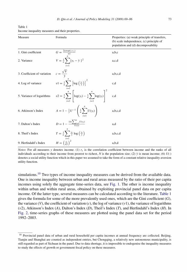
Table 1Income inequality measures and their properties.

Measure Formula Properties: (a) weak principle of transfers,(b) scale independence, (c) principle ofpopulation and (d) decomposability

1. Gini coefficient G = 2covar(y,ry)ny

a,b,c

2. Variance V = 1n

n∑i=1

[yi − y ] 2 a,c,d

3. Coefficient of variation c =√

V

ya,b,c,d

4. Log of variance v1 = 1n

n∑i=1

[log(

yi

y

)]2

c,d

5. Variance of logarithms v2 = 1n

n∑i=1

[log(yi) − 1

n

n∑i=1

log(yi)

]2

c,d

6. Atkinson’s Index A = 1 − 1yU−1

(1n

n∑i=1

U(yi)

)a,b,c,d

7. Dalton’s Index D = 1 − 1/n∑n

i=1U(yi)

U(y) a,d

8. Theil’s Index T = 1n

n∑i=1

yi

ylog(

yi

y

)a,b,c,d

9. Herfindahl’s Index H =(

yi

ny

)2a,b,d

Notes: For all measures y denotes income. (1) ry is the correlation coefficient between income and the ranks of allindividuals according to their income from poorest to richest, N is the population size; (2) y is mean income; (6) U(·)denotes a social utility function which in this paper we assumed to take the form of a constant relative inequality aversionutility function.

simulations.10 Two types of income inequality measures can be derived from the available data.One is income inequality between urban and rural areas measured by the ratio of their per capitaincomes using solely the aggregate time-series data, see Fig. 1. The other is income inequalitywithin urban and within rural areas, obtained by exploiting provincial panel data on per capitaincome. Of the latter type, several measures can be calculated according to the literature. Table 1gives the formula for some of the more prevalently used ones, which are the Gini coefficient (G),the variance (V), the coefficient of variation (c), the log of variance (v1), the variance of logarithms(v2), Atkinson’s Index (A), Dalton’s Index (D), Theil’s Index (T), and Herfindahl’s Index (H). InFig. 2, time-series graphs of these measures are plotted using the panel data set for the period1992–2003.

10 Provincial panel data of urban and rural household per capita incomes at annual frequency are collected. Beijing,Tianjin and Shanghai are counted as independent entries, but Chongqing, a relatively new autonomous municipality, isstill regarded as part of Sichuan in the panel. Due to data shortage, it is impossible to endogenise the inequality measuresto study the effects of growth or government fiscal policy on these measures.


Fig. 2. Urban, rural and overall inter-provincial per capita income inequality.


Four basic properties are commonly used to evaluate income inequality measures (e.g. seeChakravarty, 1999; Cowell, 1995; Deininger & Squire, 1998; Fields, 2001).11 These propertiesare widely known as ‘anonymity’, ‘population homogeneity’, ‘transfer principle’, and ‘incomehomogeneity’ or ‘normalization’.12 ‘Anonymity’ means that the names of the individuals areirrelevant to the question of inequality. ‘Population homogeneity’ means that when one incomedistribution is an n-fold replication of another, the two distributions would be regarded asequal. ‘Transfer principle’ means that an income transfer from a rich person to a poor personthat does not make the poor the richer of the two, reduces inequality. ‘Income homogeneity’means that a relative inequality measure is scale invariant or homogeneous of degree zero inincomes.13

In the modeling experiment, we consider only c, A, T, the three measures which satisfy all fourproperties (see Table 1). In particular, we incorporate them into the model through the privateconsumption equations, similar to what Qin (2003) has done. The consumption equations are ofthe form:

PCONit = f (PCINCit, IR%t , P#Ct,PCINCut

PCINCrt

, INEQrt, INEQut) i = r, u (1)

where PCON denotes per capita consumption, PCINC denotes per capita income, P#Cdenotes the consumer price index, INEQ denotes income inequality measures, IR% denotesthe interest rate on demand deposits, the subscript i denotes subgroup of rural and urbanhouseholds, and t denotes time. To get rid of the scale factors, we assume there are log-linear relationships between the variables, except for the interest rate and income inequalityvariables.

The effect of income inequality on consumption (and therefore savings) is of uncer-tain sign a priori, see, e.g. (Ray, 1998). If marginal savings increase with income, then anincrease in income inequality, insofar as it is equivalent to a transfer of income to the rel-atively rich, will mean an increase in aggregate savings ceteris paribus. On the other hand,if marginal savings decrease with income, an increase in income inequality could lowersavings.

In practice, regressions directly based on the log-linear form of (1) risks nonsense resultsdue to the nonstationarity of most economic time series. Hence, we adopt the general → specificdynamic modeling approach, e.g. see (Hendry, 1995). Specifically, we start with an autoregressivedistributed-lag model based on (1), gradually reduce and re-parameterize it into a parsimonious,data-congruent and economically interpretable ECM. Statistical diagnostic tests, parameter con-stancy tests, and economic interpretability of individual coefficients are used extensively as themain criteria in the model reduction.14

11 Cowell (1995) identifies an additional property—strong principle of transfers. An inequality measure satisfies thisproperty if any transfer of income from a “rich” household to a “poor” one generates a reduction in inequality that increasesas the distance between the two households’ incomes increases.12 These are sometimes referred to as ‘weak principle of transfers’, ‘principle of population’, ‘decomposability’, and

‘income scale independence’, respectively.13 Absolute inequality and relative inequality are not alternative measures of the same underlying concepts; they measure

fundamentally different concepts. Absolute inequality relies on dollar differences in real incomes. By contrast, relativeinequality is measured in terms of income ratios.14 The softwares PcGive 10.0 and PcGETS 1.0 are used in the model reduction and estimation (see Doornik & Hendry,

2001).


5. Econometric model results

As mentioned above, three income inequality measures, c, A, T, are chosen to be experimented.A simple smoothing method is used to interpolate these annual measures into quarterly series.Through modeling experiments, Theil’s index, T, is chosen as the inequality measure in themodel as it gives the most parsimonious model of the three, though the results using the other twomeasures are not so dissimilar. The sample size is 1992Q1–2003Q4.

Tables 2 and 3 present the resulting two consumption equations based on (1) together with theoriginal equations and the relevant diagnostic test statistics.15 The original equations are simplyformulated without the inequality measures, i.e.:

PCONit = f (PCINCit, IR%t , P#Ct) i = r, u (2)

A number of interesting observations are discernible from the tables. First, the encompassingtest statistics show that the inclusion of income inequality measures improves the equations signif-icantly. Second, changes in Theil’s inequality measures are found to exert only short-run impact.These two results corroborate the classical finding, e.g. (Staehle, 1937, 1938) that income inequal-ity cannot be ignored in determining aggregate consumption, especially when income inequalityevolves over time. Noticeably, urban and rural households react to the changing gap between urbanand rural inequality measures and, in addition, urban households also react to changes in urbanincome inequality. The short-run, positive reaction of rural households towards consumption withrespect to increasing income inequality may be explained by the fact that the rural householdsbecame more dependent on cash consumption rather than self-sustained consumption. Finally, anincrease in average income level of the urban/rural households relative to the rural/urban house-holds is found to exert significantly negative long-run impact on the urban/rural consumption. Thissuggests that urban/rural households exhibit a greater savings motive when they perceive theirincome growing steadily faster than their rural/urban counterparts. This result partly confirmsthe theory that inequality affects long-run aggregate demand negatively (see Zweimüller, 2000).

Of course, it cannot be inferred that income inequality is harmful for long-run aggregatedemand by looking at the consumption effects alone. One also needs to take into account theeffect of income inequality – even indirect ones – on the other variables. For instance, suppressedconsumption will raise savings and hence may encourage investment, and eventually enhancefuture consumption. To investigate the overall macroimpact of income inequality, we carry out anumber of model simulations.

6. Model simulations

Two sets of simulations are carried out using two model versions, one in which the twoconsumption equations are without inequality measures (Model 1 in Tables 2 and 3) and the otherin which the two equations are with the measures (Model 2 in Tables 2 and 3).16 The base runassumes that income inequality is constant at the 2003Q4 level from the beginning of 2004 up tothe end of the simulation period, which covers 2005Q1–2010Q4.17

15 The original equations are from the 2004 version of the model, which is also used for the later simulations. The modelpresented in (Qin et al., 2007) contains some modifications of that version.16 The simulations are carried out using WinSolve, see Pierse (2001) for a detailed description of the software.17 The simulations start from 2005Q1 to avoid the periods where there are already actual values for the variables of

interest, even though the data series of the inequality measures end at 2003Q4.

D.Q

inetal./JournalofPolicy

Modeling

31(2009)

69–8677

Table 2Per capita consumption of urban household.

Without income inequalitymeasure (Model 1)

�2 ln(PCONu)t = −0.0644(0.0301)

− 0.0419(0.0138)

× (SQ1 + SQ2) − 0.3761(0.1006)

× �2 ln(PCONu)t−2

+ 0.4562(0.0733)

× �2 ln(PCINCu)t + 0.2573(0.1032)

× �4ln(P#C)t

− 0.5172(0.1126)

×(

lnPCONu

PCINCu+ 0.005 × (IR% − 100 × �4 ln(P#C))

)t−2

Residual diagnostics σ (standard error) 0.0245413No autocorrelation F(3,32) = 1.5187 [0.2285]Normality χ2(2) = 3.2946 [0.1926]Homoscedasticity F(9,25) = 1.7550 [0.1285]RESET F(1,34) = 1.5233 [0.2256]

With income inequality measure(Model 2)

�2 ln(PCONu)t =−0.0305

(0.0107)− 0.3854

(0.0751)× �2 ln(PCONu)t−2 − 0.0341

(0.0139)× SQ2 − 0.0612

(0.0185)× SQ3 + 0.3742

(0.0523)

× �2ln(PCINCu)t + 0.2628(0.0608)

× �4 ln(PCINCu)t−1 + 0.5805(0.1109)

× �2�4 ln(P#C)t + 18.5771(6.306)

× ��(INEQu − INEQr)t−1 − 43.72(11.10)

× ��INEQut−1 − 0.7333(0.0752)

×[

lnPCONu

PCINCu+ 0.005 × (IR% − 100 × �4 ln(P#C))−1 + 0.13 × ln

(PCINCu

PCINCr

)−1

]t−2

Residual diagnosticsNo autocorrelation F(3,28) = 1.6566 [0.1989]Normality χ2(2) = 0.4401 [0.8025]Homoscedasticity F(16,14) = 1.3718 [0.2790]RESET F(1,30) = 0.9166 [0.3460]

Encompass-ing test Model 1 vs. Model 2 Model 2 vs. Model 1Cox N(0,1) = −8.620 [0.0000]a N(0,1) = −0.4500 [0.6527]Ericsson IV N(0,1) = 5.032 [0.0000]a N(0,1) = 0.1229 [0.7023]Sargan χ2 (7) = 18.859 [0.0086]a χ2 (3) = 0.92356 [0.8197]Joint Model F(7,28) = 4.6736 [0.0014]a F(3,28) = 0.2866 [0.8347]

Note: The variable notations are given in Appendix A. Δ2 denotes second-order difference, i.e. xt − xt−2. SQ denotes quarterly seasonal dummy. The statistics in the bracketsbelow coefficient estimates are standard errors. The statistics in the squared brackets following test statistics are the associated probabilities.

a Probability is smaller than 1%, i.e. strongly rejecting the null hypothesis.

78D

.Qin

etal./JournalofPolicyM

odeling31

(2009)69–86

Table 3Per capita consumption of rural household.

Without income inequalitymeasure (Model 1)

�3ln(PCONr)t = −0.4190(0.0390)

+ 0.3226(0.0218)

× SQ1 − 0.0064(0.002)

× �3(IR% − 100 × �4 ln(P#C))t

+ 0.0113(0.0041)

× �(IR% − 100 × �4ln(P#C))t−3 + 0.5159(0.0323)

× �3ln(PCINCr)t + 0.1367(0.0218)

× � ln(PCINCr)t−2 − 0.5971(0.0605)

×(

lnPCONr

PCINCr+ 0.007 × (IR% − 100 × �4ln(P#C))

)t−3


With income inequality measure(Model 2)

�3ln(PCONr)t = −1.0056(0.0629)

+ 0.2338(0.0329)

× SQ1 − 0.0095(0.0017)

× �3(IR% − 100 × �4 ln(P#C))t

+ 0.0058(0.0016)

× �3(IR% − 100 × �4 ln(P#C))t−3 + 0.3755(0.0257)

× ��3ln(PCINCr)t + 0.3537(0.0592)

× �3

(ln

PCINCr

PCINCu

)t−1

+ 0.1525(0.0258)

× �

(ln

PCINCr

PCINCu

)t−2

+ 16.939(6.059)

× �(INEQr − INEQu)t

− 0.9921(0.0615)

×(

lnPCONr

PCINCr+ 0.008 × (IR% − 100 × �4ln(P#C)) + 0.4 ×

(ln

PCINCr

PCINCu

))t−3


Encompass-ing test Model 2 vs. Model 1Cox Model 1 vs. Model 2 N(0,1) = -0.5074 [0.6119]Ericsson IV N(0,1) = −6.590 [0.0000]a N(0,1) = 0.4279 [0.6687]Sargan N(0,1) = 3.871 [0.0001]a χ2 (4) = 2.5040 [0.6439]Joint Model χ2 (6) = 15.470 [0.0169]* F(4,25) = 0.5907 [0.6725]

F(6,25) = 4.1504 [0.0050]a

Note: The variable notations are given in Appendix A. Δ2 denotes second-order difference, i.e. xt − xt−2. SQ denotes quarterly seasonal dummy. The statistics in the bracketsbelow coefficient estimates are standard errors. The statistics in the squared brackets following test statistics are the associated probabilities.

a Probability is smaller than 1%, i.e. strongly rejecting the null hypothesis.* Indicates the probability being smaller than 5% but larger than 1%.


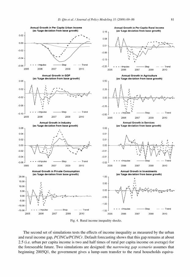
The first set of simulations is the conventional impulse, step, and trend shocks on each of theurban and rural inequality measures. These shocks are defined below.

1. Impulse shock refers to an increase in inequality for 1 year (2005Q1–2005Q4) by 10% fromits 2003Q4 level; then it returns to the 2003Q4 level at 2006Q1 and remains so to the end ofthe simulation period.

2. Step shock refers to an increase in inequality by 10% from its 2003Q4 level at 2005Q1, andremains so to the end of the simulation period.

3. Trend shock refers to a linear increase in inequality at 10% per annum starting from 2005Q1.The growth rate is chosen with reference to the increase in overall Theil index during recentyears, e.g. 9% in 2002 and 13% in 2003.

Notice that INEQu and INEQr, the inequality measures, are calculated from panel data whereasPCINCu and PCINCr, the household per capita income series, are taken from China MonthlyEconomic Indicators. Therefore, the shocks defined above implicitly assume that changes inINEQu and INEQr do not affect PCINCu and PCINCr directly. However, as the income vari-ables are endogenous in the model, they are impacted indirectly by changes in the inequalitymeasures. Hence, the only assumption we make is that the shocks do not affect the incomelevels at the initial point when they first occur. In Figs. 3 and 4, the indirect effect of theshocks on PCINCu and PCINCr are plotted (top panels). It is interesting to see that increas-ing urban inequality would, to a large extent, stimulate the growth of both urban and rural incomelevel, whereas both urban and rural incomes would decline with increasing rural inequality.More interestingly, rural household income growth would not be significantly affected down-wards if the inequality situation keeps evolving at the present pace (the trend shock case),i.e. unless there is an abrupt deterioration in income inequality (the impulse and step shockcases). Nevertheless, this result highlights the need, at the macro-level, to address rural incomeinequality.

Figs. 3 and 4 also demonstrate, for the urban and rural sectors respectively, the effects ofthe inequality shocks on GDP, its supply side components of the three-sector output, and itsdemand-side components of private consumption and capital formation, all measured in constantprice. In the urban scenario (Fig. 3), rural inequality is assumed to remain at its 2003Q4 levelthroughout the simulation period. The same applies to the rural scenario (Fig. 4). It can be seenthat the overall effects of rising inequality on GDP growth are almost negligibly small. In theurban scenario, rising inequality appears to stimulate slightly the industry and services sectors.Agriculture seems to be the only sector that would get virtually no long-run benefit. In comparison,agriculture is slightly worse off and the other two sectors are significantly worse off in the ruralscenario.

From the demand-side of GDP, private consumption is the most responsive to income inequalityshocks in terms of both velocity and volatility, with the response rapidly tapering off to virtuallyzero. This is not surprising given the household consumption equations reported in Tables 2 and 3.The volatility in aggregate consumption undulates on to aggregate investment, whose responsesoscillate more persistently and more strongly than those of the three sectors. In a recent studyby Qin, Cagas, He, and Quising (2006), impulse shocks in investment are found to affect theoutput growth in the industry and services sectors far more than that of the agricultural sector.This helps to explain why the output growth of the three sectors responds very differently tothe inequality shocks. If judged by economic stability, the simulation results show that changinginequality adversely affects the stability by encouraging more volatility in the growth of aggregateconsumption, investment, and GDP.


Fig. 3. Urban income inequality shocks.


Fig. 4. Rural income inequality shocks.

The second set of simulations tests the effects of income inequality as measured by the urbanand rural income gap, PCINCu/PCINCr. Default forecasting shows that this gap remains at about2.5 (i.e. urban per capita income is two and half times of rural per capita income on average) forthe foreseeable future. Two simulations are designed: the narrowing gap scenario assumes thatbeginning 2005Q1, the government gives a lump-sum transfer to the rural households equiva-


Fig. 5. Rural–urban income gap shocks.


lent to 1% of the previous year’s GDP; the widening gap scenario assumes that the governmenttaxes the rural household income an amount equivalent to 1% of the previous year’s GDP.18

The two scenarios amount to shifting the existing income gap by 0.15 roughly during the sim-ulation period, as shown in Fig. 5. It is clear from the figure that, for the most part, the twoscenarios result in opposite effects. Narrowing the income gap has an immediate and sustainedpositive impact on GDP growth, whereas widening the gap has a negative immediate effect thateventually tapers off and becomes positive towards the end of the simulation period. On thewhole, the narrowing-gap scenario results in weaker macroeconomic responses in terms of mag-nitude as rural households have a smaller share of aggregate private consumption than urbanhouseholds.

In terms of dynamics, the step shocks of changing urban and rural income gaps affect privateconsumption almost immediately and very significantly, and in turn its responses are transmittedto investment, agricultural production, industrial production and services supply. The narrowing-gap scenario initially boosts aggregate private consumption by up to around 2.7% in the shortrun, whereas the widening-gap scenario depresses it, and both effects recede quickly to about0.15–0.19% in absolute value in the long run. Consumption responses in turn are transmitted todemand for sectoral output, especially for agricultural produce and services, and these undulateon to investment demand. Notice that the responses of the secondary sector follow closely thoseof investment, only on a smaller scale, as this is the sector most dependent on investment. Incomparison, the primary and tertiary sectors are more demand-driven. Hence their growths arebuoyed by the increase in disposable income in the narrowing-gap scenario, and vice versa in thewidening-gap scenario.

Compared to the first set of simulations, the results of the second set show that furtherwidening of rural–urban income inequality would hinder economic growth, while narrowingthe inequality would actually boost long-run growth. Overall, the simulations suggest thatfurther disparate income distribution is unlikely to contribute favorably to sustaining steady eco-nomic growth, even though the likely adverse impact may not yet be very significant at themacro-level.

7. Conclusion

Macroeconometric models are incapable of tackling the issue of how income inequality affectsgrowth empirically for lack of explicit channels relating aggregate income and consumption toincome distribution. The present study runs a pilot experiment to incorporate panel data infor-mation into a macro-econometric model of China so that the issue of how income inequalityaffects growth can be studied through model simulations. A panel of provincial urban and ruralhousehold income data is used to construct income inequality measures, which are used to aug-ment the urban and rural consumption equations of the China model. Simulations are then carriedout on the modified model to see how future changes in income inequality would affect themacro-economy.

Through model augmentation, the rapidly changing income inequality is found to exertsignificant impact on consumption of both urban and rural households. While rising urbanincome inequality holds back urban consumption in the short run, increase in the relative

18 The simulations implicitly assume that the taxes and transfers are proportional to household incomes so that within-urban and within-rural inequalities are unaffected.


income level between rural and urban areas is found to stimulate household savings in thelong run.

Through model simulations, we observe several interesting results. We find that significantchanges in income inequality – whether within-urban, within-rural, or urban–rural – carry negativeeffects on macro-economic stability as they cause consumption and then investment to undulate.Comparing the effects of shocking each of the urban and rural inequality measures, we find thatincreases in urban inequality carry more favorable (or less negative) effects than increases inrural inequality. In simulating the impact of changing urban–rural average income disparity, wesee that long-run GDP growth is highest when urban–rural income gap is narrowed (i.e. rural-favorable growth), as compared with the scenario where it is widened, and that the urban-favorablegrowth scenario (i.e. widening urban–rural gap) would only benefit the industrial sector in thelong run.

These results carry significant policy implications. Specifically, our findings indicate thatanti-inequality policies should prioritize narrowing the urban–rural income gap and alleviatingwithin-rural area inequality. Policies fostering economic growth in the rural areas augmentedby rural social welfare provision, such as on education and health care, are examples of suchpolicies. Policies facilitating greater labour mobility should also be considered to further uti-lize the agricultural labour surplus, see also (Besley & Burgess, 2003) for more discussionon relevant policy measures. More fundamentally, our findings show the imperative of havinganti-inequality policies high on the agenda, not just for economic growth, but for social stabil-ity, as widening income inequality in any respect is found to have economically destabilizingeffect.

Several extensions of the present study are desirable. First, it is desirable to extend the fiscalblock of the model to establish explicit links between income inequality and income re-distributionpolicies. Secondly, it is desirable to extend the consumption block to base it on panel data entirelyso as to achieve data consistency between aggregate income levels and income inequality mea-sures. Thirdly, it is desirable to explore explicit links between income inequality and employmentdistribution among the three sectors of GDP. More data would be needed for this extension.Whichever direction of extension, a wider mix of time-series and panel data in macroeconometricmodeling seems the desirable way forward.

Acknowledgements

Thanks are due to many of the colleagues at ADB and IWEP of CASS, who offered us varioussuggestions and support. We are also grateful for the suggestions from participants at EcoMod2005 Conference, where the original version of the paper was presented, and for the commentsfrom the referee and the editor of JMP.

Appendix A. Main data sources and variable definition

National Bureau of Statistics: Statistics Yearbook of China (SYC), China Monthly Eco-nomic Indicators (CMEI), Comprehensive Statistical Data and Materials on 50 years of NewChina (1999, CSDM). Some of the historical data are from National Bureau of Statisticsdirectly.


Variables Definition Source

GDPc Gross domestic product, quarterly frequency (million yuan, in 1992Q1price)

CMEI

INEQu, INEQr Income inequality measures, quarterly frequency interpolated fromannual data (Theil’s index is the final choice)

Own calculation

IR% Interest rate on demand deposits, quarterly frequency CMEIP#C Consumer price index, quarterly frequency 1992Q1 = 100 CMEIPCINCri Provincial per capita net income of rural households of China, annual

frequency (yuan)CSDM

PCINCr Per Capita net income of rural households of China, quarterlyfrequency (yuan)

CMEI

PCINCui Provincial per capita disposable income of urban households of China,annual frequency (yuan)

CSDM

PCINCu Per capita disposable income of urban households of China (yuan) CMEIPCONr Per capita living consumption of rural households of China, quarterly

frequency (yuan)CSDM & CMEI

PCONu Per capita living consumption of urban households of China, quarterlyfrequency (yuan)

CSDM & CMEI

POPr Population of rural China, annual frequency (1000 persons) SYCPOPri Provincial population of rural China, annual frequency (1000 persons) CSDMPOPu Population of urban China, annual frequency (1000 persons) SYCPOPui Provincial population of urban China, annual frequency (1000 persons) CSDM

References

Aghion, P., Caroli, E., & Garcia-Penalosa, C. (1999). Inequality and economic growth: The perspective of the new growththeories. Journal of Economic Literature, 37, 1615–1660.

Alesina, A., & Rodrik, D. (1994). Distributive politics and economic growth. The Quarterly Journal of Economics, 109,465–489.

Bagliano, F.-C., & Bertola, G. (2004). Models for dynamic macroeconomics. Oxford: Oxford University Press.Benabou, R. (1996). Inequality and growth. In B. Bernanke & J. Rotemberg (Eds.), NBER Macro-Annual 1996 (pp.

11–76). Cambridge: MIT Press.Benjamin, D., Brandt, L., & Giles, J. (2004). The evolution of income inequality in China. William Davidson institute

working papers series, 654.Besley, T., & Burgess, R. (2003). Halving global poverty. Journal of Economic Perspective, 17, 3–22.Bourguignon, F. (1981). Pareto-superiority of unegalitarian equilibria in Stiglitz’ model of wealth distribution with convex

savings function. Econometrica, 49, 1469–1475.Bourguignon, F., Pereira, L. A., & Silva, D. (2003). The impact of economic policies on poverty and income distribution:

Evaluation techniques and tools. Oxford: Oxford University Press.Chakravarty, S. R. (1999). Measuring inequality: The axiomatic approach. In J. Silber (Ed.), Handbook of income inequality

measurement (pp. 163–186). Boston/Dordrecht/London: Kluwer Academic Publishers.Chen, S., & Wang, Y. (2001). China’s growth and poverty reduction: Recent trends between 1990 and 1999. World Bank

policy research working paper no. 2651.Cowell, F. A. (1995). Measuring inequality. London: Prentice Hall-Harvester Wheatsheaf.Deininger, K., & Squire, L. (1998). New ways of looking at old issues. Journal of Development Economics, 57, 259–287.Doornik, J. A., & Hendry, D. F. (2001). Empirical econometric modeling using PcGive. London: Timberlake Consultants

Ltd.Fields, G. S. (2001). Distribution and development: A new look at the developing world. Cambridge, MA: Russell Sage

Foundation and MIT Press., pp. 1–72, 191–224.Figini, P. (1999). Inequality and growth revisited. Trinity College Dublin Economics Department: Economic Papers, 99/2.Galor, O., & Tsiddon, D. (1997). Technological progress, mobility, and economic growth. American Economic Review,

87, 363–382.Galor, O., & Zeira, J. (1993). Income distribution and macroeconomics. Review of Economic Studies, 60, 35–52.


Hendry, D. F. (1995). Dynamic econometrics. Oxford: Oxford University Press.Kaldor, N. (1956). Alternative theories of distribution. Review of Economic Studies, 23, 83–100.Kaldor, N. (1957). A model of economic growth. Economic Journal, 57, 591–624.Knack, S., & Keefer, P. (2000). Polarization, politics, and property rights: Links between inequality and growth. World

Bank policy research working paper, no. 2418.Krongkaew, M. (2003). Income distribution and sustainable economic development in east Asia: A comparative analysis.

Paper presented at annual meeting of the east Asian development network held in Singapore on October 10–11, 2003.Kuznets, S. (1955). Economic growth and income inequality. American Economic Review, 45, 1–28.Li, S., Zhang, P., Wei, Z., & Zhong, J. (2000). Positive analysis on distribution of income on China (in Chinese). Beijing:

Social Science Documentation Press., pp. 5–14.Lin, B. (2003). Economic growth, income inequality, and poverty reduction in People’s Republic of China. Asian

Development Review, 20, 105–124.Perotti, J. (1996). Growth, Income distribution and democracy: What the data say. Journal of Economic Growth, 1,

149–187.Persson, T., & Tabellini, G. (1994). Is inequality harmful for growth: Theory and evidence. American Economic Review,

84, 600–621.Pierse, R. (2001). Winsolve manual. UK: Department of Economics, University of Surrey.Qin, D. (2003). Determinants of household savings in China and their role in quasi-money supply. Economics of Transition,

11, 513–537.Qin, D., He, X.-H., Liu, S.-G., & Quising, P. (2005). Modeling monetary transmission and policy in People’s Republic of

China. Journal of Policy Modeling, 27, 157–175.Qin, D., Cagas, M. A., He, X.-H., & Quising, P. (2006). How much does investment drive economic growth in China.

Journal of Policy Modeling, 28, 751–774.Qin, D., He, X., Liu, R., Liu, S., Cagas, M. A., Ducanes, G., et al. (2007). A small macroeconometric model of China.

Economic Modelling, 24, 814–822.Ray, D. (1998). Development economics. Princeton: Princeton University Press.Robinson, J. (1933). The economics of imperfect competition. London: Macmillan.Staehle, H. (1937). Short-period variations in the distribution of income. Review of Economic Statistics, 19, 133–143.Staehle, H. (1938). New considerations on the distribution of incomes and the propensity to consume. Review of Economic

Statistics, 20, 134–141.World Bank. (1997). Sharing rising incomes. Washington, DC.Zhang, P. (2003). Growing and sharing income distribution theory, events and policy. Beijing: Social Science Documen-

tation Press., p. 16.Zhang, X., & Kanbur, R. (2005). Spatial inequality in education and health care in China. China Economic Review, 16,

189–204.Zweimüller, J. (2000). Inequality, redistribution and economic growth. Institute for empirical research in economics

working paper no. 31. University of Zurich.

effects of income inequality on china’s economic growth

Documents