effect of gis learning on spatial ability
TRANSCRIPT

EFFECT OF GIS LEARNING ON SPATIAL ABILITY
A Dissertation
by
JONG WON LEE
Submitted to the Office of Graduate Studies of Texas A&M University
in partial fulfillment of the requirements for the degree of
DOCTOR OF PHILOSOPHY
May 2005
Major Subject: Geography
EFFECT OF GIS LEARNING ON SPATIAL ABILITY
A Dissertation
by
JONG WON LEE
Submitted to Texas A&M University
in partial fulfillment of the requirements for the degree of
DOCTOR OF PHILOSOPHY
Approved as to style and content by: _____________________________
Robert Bednarz (Co-Chair of Committee)
_____________________________
Sarah W. Bednarz (Co-Chair of Committee)
_____________________________Hongxing Liu
(Member)
_____________________________Lynn M. Burlbaw
(Member)
_____________________________Douglas J. Sherman
(Head of Department)
May 2005
Major Subject: Geography

iii
ABSTRACT
Effect of GIS Learning on Spatial Ability. (May 2005)
Jong Won Lee, B.A., Seoul National University;
M.A., Seoul National University
Co-Chairs of Advisory Committee: Dr. Robert Bednarz Dr. Sarah W. Bednarz
This research used a spatial skills test and cognitive-mapping test to examine the
effect of GIS learning on the spatial ability and spatial problem solving of college
students. A total of 80 participants, undergraduate students at Texas A&M University,
completed pre- and post- spatial skills tests administered during the 2003 fall semester.
Analysis of changes in the students’ test scores revealed that GIS learning could help
students improve their spatial ability. Strong correlations existed between the
participants’ spatial ability and their performance in the GIS course. The research also
found that spatial ability improvement linked to GIS learning was not significantly
related to differences in gender or to academic major (geography majors vs. science and
engineering majors).
A total of 64 participants, recruited from students enrolled in Introduction to GIS
and Computer Cartography at Texas A&M University, completed pre- and post-
cognitive-mapping tests administered during the 2003 fall semester. Students’
performance on the cognitive-mapping test was used to measure their spatial problem
solving. The study assumed that the analysis of the individual map-drawing strategies
would reveal information about the cognitive processes participants used to solve their
iv
spatial tasks. The participants were requested to draw a map that could help their best
friends find their way to three nearby commercial locations. The map-drawing process
was videotaped in order to allow the researcher to classify subjects’ map-drawing
strategies. The study identified two distinctive map-drawing strategies: hierarchical and
regional. Strategies were classified as hierarchical when subjects began by drawing the
main road network across the entire map, and as regional when they completed mapping
sub-areas before moving on to another sub-area. After completion of a GIS course, a
significant number of participants (about half) changed their map-drawing strategies.
However, more research is necessary to address why these changes in strategy came
about.

v
DEDICATION
To my loving wife Jong Ok
You are my rock, you are my love.

vi
ACKNOWLEDGEMENTS
I would like to acknowledge all the people who have helped me to complete the
work for this degree. I am most grateful for the guidance I received from each of my
committee members: Dr. Robert Bednarz, Dr. Sarah Bednarz, Dr. Hongxing Liu, and Dr.
Lynn Burlbaw. Their support and expertise were essential in the progress and
completion of my dissertation study.
Special thanks go to Drs. Robert Bednarz and Sarah Bednarz who served as co-
chairs of my dissertation committee. Thank you, Bob, for serving as my mentor since we
met for the first time in 2000 at Seoul. You have always been there to respond quickly to
my questions and to provide advice into what I needed to do. And thank you, Sarah, for
always being such a positive person and for all of your support while I studied in
College Station. Your encouragement and caring attitude have helped me immeasurably
to attain my ultimate goal.
I extend a special thanks to Dr. Anthony Filippi, Dr. Andrew Klein, Dr. Daniel Sui,
Dr. So-min Cheong, Dr. Douglas Sherman, Matthew Clemonds, Alexis Green, and
Jeatawn Degelia for their assistance in data collection.
I would also like to thank my friends and colleagues Dr. Gillian Acheson, Sandra
Metoyer, and Jose Gavinha for reviewing my manuscripts and providing valuable advice.
To Jose, your input has been influential in the “finishing” of this dissertation.
Last but not least, I would like to express my sincere gratitude to my wife and best
friend, Jong Ok, for all her encouragement to pursue this degree and her endless patience
and support throughout the process. Your love and strength are limitless and I am

vii
cherishing every moment in the journey we travel together. Also, I would like to thank
my daughter Soyoon, your smiles and babbles have lightened my life the past two years
and gave me the ultimate push to finish my work.

viii
TABLE OF CONTENTS
Page
ABSTRACT. .................................................................................................................... iii
DEDICATION . .................................................................................................................v
ACKNOWLEDGEMENTS . ............................................................................................vi
TABLE OF CONTENTS. .............................................................................................. viii
LIST OF FIGURES...........................................................................................................xi
LIST OF TABLES. ..........................................................................................................xii
CHAPTER
I INTRODUCTION ............................................................................................1
Context of Research Problem..................................................................1 GISystem and GIScience .........................................................2 GIS Learning ............................................................................3 Spatial Ability in the Use of GIS .............................................4 Cognitive Mapping for Spatial Problem Solving.....................6
Research Questions .................................................................................7 Research Methods ...................................................................................9 Study Significance.................................................................................10 Study Assumptions................................................................................12 Study Limitations ..................................................................................12
II REVIEW OF LITERATURE........................................................................13
Analytical and Visual Features of GIS..................................................13 Analytical Processes in GIS ...................................................13 Visualization in GIS ...............................................................17
Spatial Ability .......................................................................................20 Definition of Spatial Ability...................................................20 Measurement of Spatial Ability .............................................22 Individual Differences in Spatial Ability ...............................25 GIS Learning and Spatial Ability...........................................27
Cognitive Mapping and Problem Solving.............................................28 Mechanical Approach ............................................................29 Structural Approach ...............................................................31
ix
CHAPTER Page
Process-Oriented Approach....................................................33 How People Draw a Map: Map-drawing Strategy .................35
Relationship between Aptitude and Strategy Choice............................40 Summary ...............................................................................................42
III RESEARCH METHODOLOGY.................................................................45
Experiment 1: Spatial Skills Test .........................................................45 Test Descriptions....................................................................45 Subjects and Test Setting .......................................................50 Test Administration................................................................53 Data Scoring and Analysis .....................................................53
Experiment 2: Cognitive-Mapping Test................................................54 Research Questions ................................................................54 Subjects ..................................................................................55 Test Descriptions and Procedure............................................55 Pilot Tests ...............................................................................57 Analysis ..................................................................................58
IV FINDINGS AND ANALYSIS.....................................................................59
Experiment 1: Spatial Skills Test ..........................................................60 Test Reliability .......................................................................60 Score Comparison by Group ..................................................60 Score Comparison by Gender and Major ...............................66 Correlation between the Spatial Skills Test and GIS Course Achievement...........................................................................70
Experiment 2: Cognitive-Mapping Test................................................72 Video-Analysis of Map-drawing Strategy .............................72 Classification of Map-drawing Strategy ................................75 Quantitative Comparison among Strategies...........................84 Changes of Map-drawing Strategies ......................................86 Relationship between Map-drawing Strategy and Spatial Ability.....................................................................................89
V DISCUSSION AND CONCLUSIONS.........................................................91
Research Question 1a ............................................................................92 Research Question 1b............................................................................96 Research Question 1c ............................................................................98
Educational Implications: GIS Lab Exercise, Project, and Their Relationship ................................................................101

x
Page Research Question 2a ..........................................................................104 Research Question 2b..........................................................................106 Summary and Conclusions..................................................................109 Suggestions for Future Research.........................................................113
REFERENCES...............................................................................................................115 APPENDIX 1 .................................................................................................................142 APPENDIX 2 .................................................................................................................162 VITA ..............................................................................................................................166

xi
LIST OF FIGURES
FIGURE Page
1 GIS activities and spatial abilities ........................................................................6
2 The sequential and spatial map from Applyard (1970)......................................32
3 Number of GIS courses completed by the subjects and their average scores in the spatial skills test ......................................................................................50 4 Reference map....................................................................................................56
5 A comparison of pre- and posttest scores by group ...........................................61
6 Score changes of pre- and posttest by gender ....................................................67
7 Score changes in pre- and posttest by major......................................................69
8 Maps created based in a regional (A) and a hierarchical (B) approach. ............74
9 Hierarchical approach 1 (major and secondary roads drawn before features)...76
10 Hierarchical approach 2 (major roads first, then each secondary road and associated features). ...........................................................................................77 11 Regional approach (one area at a time, without a major road network) ............78
12 Mixed approach..................................................................................................79
13 Relationship between GIS activities and spatial abilities. .................................93

xii
LIST OF TABLES
TABLE Page
1 Three types of spatial analytical methods of GIS ..............................................15
2 Average scores and standard deviations in the pilot test....................................50
3 Control group and three experimental groups....................................................51
4 The type of quasi-experimental design used in experiment 1............................53
5 A comparison of pre- and posttest scores by group ...........................................61
6 ANOVA for pretest scores by group..................................................................62
7 ANCOVA using posttest scores as the dependent variable with the pretest scores as the covariate........................................................................................63 8 Paired sample t-test for gain scores....................................................................64
9 Average scores and standard deviations by item type .......................................65
10 Effect of the completion of Physical Geography on the spatial skills test.........66
11 A comparison of pre- and posttest scores by gender..........................................67
12 ANCOVA using posttest scores as the dependent variable with the pretest scores as the covariate (by gender) ....................................................................68 13 A comparison of pre- and posttest scores by major ...........................................69
14 ANCOVA using posttest scores as the dependent variable and the pretest scores as the covariate (by major)......................................................................70 15 Correlation between spatial skills test and performance of GIS course.............71
16 A comparison of pre- and posttest scores by assignment type ..........................71
17 ANCOVA using posttest scores as the dependent variable and the pretest scores as the covariate (by assignment type) .....................................................72 18 The mean second required for each map-drawing strategy used by the subjects (pretest only) ........................................................................................85

xiii
TABLE Page
19 Map-drawing strategy by gender and major (pretest only)................................85 20 Map-drawing strategies in the pre- and posttest ................................................86
21 Direction of map-drawing strategy changes ......................................................87
22 A comparison of posttest scores by map-drawing strategies .............................90
23 ANOVA for posttest scores by map-drawing strategies ....................................90

1
CHAPTER I
INTRODUCTION
Context of Research Problem
This study investigates the effects of GIS learning on spatial abilities and spatial
problem solving of college students. It has been suggested that GIS can help students
develop spatial abilities (Albert and Golledge 1999; Self et al. 1992), solve spatial
problems (Audet and Abegg 1996; Audet et al. 1993; Audet and Paris 1997; Baker 2000;
Barstow 1994; Hall-Wallace and McAuliffe 2002; Kerski 2000; Salinger 1995;
Wigglesworth 2000), reason spatially (ESRI 1996; Geography Education Standards
Project 1994; Hagevik 2003; UCGIS 1997), improve higher-order thinking skills
(Ramirez 1995a; Sanders et al. 2001; West 2003), enhance map-reading skills (Forer and
Unwin 1999), and learn geographic principles (Patterson et al. 2003).
Despite many claims that learning GIS improves spatial abilities, results are
inconsistent concerning both the existence and magnitude of the effects of GIS learning
on spatial ability. For example, Kerski (2000) reported that high school students using
GIS scored significantly higher than students using traditional methods on a spatial
analysis test. Furthermore, the GIS group demonstrated better abilities to synthesize,
identify, and describe human and physical patterns. In research examining how students’
spatial abilities affect the understanding of environmental content after using GIS,
This dissertation follows the style of Journal of Geography.

2
Hagevik (2003) concluded that learning with GIS developed students’ spatial-visual
thinking skills. A study by Baker (2002) concluded that students showed improvement in
integrating science process skills after a two-week GIS treatment. However, GIS
students in the same study did not improve their ability to recognize geographic patterns
and make generalized statements about the trends in the data. This finding confirmed
research by Abbott (2001), who did not find a significant difference between students in
an experimental GIS group and the control group in a test of integrated scientific process
skills. A study by Albert and Golledge (1999) also did not find significant differences
between GIS-users and non-users in subjects’ abilities to use map overlays. A brief
description of major concepts used in this study follows.
GISystem and GIScience
There has been extensive debate over whether the “S” of GIS should be interpreted
as system (GISystem) or science (GIScience) (Forer and Unwin 1999; Kemp et al. 1992;
Longley et al. 2001; Wright et al. 1997). GISystem focuses on technology for the
acquisition and management of spatial information (Forer and Unwin 1999). According
to Wright et al. (1997), “doing GIS” is differentiated from “doing GISc” as follows:
[Doing GIS] is identified as a problem solving activity, while science was linked to discovery and problem understanding … (Wright et al. 1997, 349).
Doing GIS amounts to making use of a tool to advance the investigation of a
problem … (Wright et al. 1997, 355). Doing GIS is not necessarily the same as “doing science” (Wright et al. 1997,
357).
Unlike GISystem, GIScience pursues a scientific approach to the fundamental issues
3
arising from geographic information (Longley et al. 2001). In this perspective, “doing
GIScience” is interpreted as follows:
[GIScience] spoke mainly about the use of GIS as a method or body of knowledge for developing and testing spatial theories, not about the physical entity GIS itself … (Wright et al. 1997, 349).
Doing GIS is “doing science” and the only sufficient grounds for legitimacy
as a research field in the academy (Wright et al. 1997, 358).
Despite considerable discussion, the distinction between GISystem and GIScience is still
not clear. In fact, some prefer a fuzzy distinction between GISystem and GIScience. For
example, Wright et al. (1997) argue that the GIS should be described along a “fuzzy”
continum rather than “black-and-white” boxes of description. According to this idea,
GIS is interpreted depending on its purpose or situation. For instance, while GIS having
technical and problem-solving orientation at the undergraduate level course is closer to a
tool or system, GIS emphasizing discovery and problem understanding at the graduate
level or for research is more likely to be science. In this study, GIS refers to both its use
as a tool and technology (GISystem), and to inference and spatial reasoning (GIScience).
GIS Learning
In order to use GIS properly, three different types of knowledge are needed:
declarative, procedural, and conditional knowledge:
Declarative knowledge is “knowing that,” or “knowing about.” It is fact, concepts, or ideas organized in different ways, as lists, as statements, or as stories. Knowing how to do something is termed procedural knowledge. Performing a series of tasks in the correct sequence requires procedural knowledge. Much of the learning involved in GIS is procedural knowledge. The third type of knowledge is termed conditional knowledge, knowing when and why to use a procedure. All three types of knowledge are required to learn and do GIS (Bednarz 1997, 197).

4
GIS leaning in this study refers to learning what GIS is, how to use it, and when and
where to use it. The purpose of this study is to examine whether the completion of a GIS
course affects spatial abilities of college students. Therefore, “GIS learning” in this study
is defined narrowly as the completion of a semester-long GIS course offered at the
undergraduate level.
Spatial Ability in the Use of GIS
Cognitive psychologists, such as McGee (1979b), generally agree that spatial
ability comprises several distinct but interrelated factors. Nevertheless, some
disagreement still exists about whether there are two dominant dimensions–spatial
visualization and spatial orientation–or whether a third–spatial relations–is also a
fundamental dimension of spatial ability (Gilmartin and Patton 1984; Golledge and
Stimson 1997; Lohman 1979; Montello et al. 1999). Spatial visualization is the ability to
mentally manipulate, rotate, twist, or invert pictorially presented visual stimuli. Spatial
orientation involves the comprehension of the arrangement of elements within a visual
stimulus pattern, the aptitude for remaining unconfused by the changing orientations in
which a configuration may be presented and the ability to determine spatial relations in
which the body orientation of the observer is an essential part of the problem (McGee
1979b). The dimension that is the least clearly defined, and the most contentious, is
spatial relations:
Spatial relations include abilities to recognize spatial distributions and spatial patterns, to connect locations, to associate and correlate spatially distributed phenomena, to comprehend and use spatial hierarchies, to regionalize, to orientate
5
to real-world frames of reference, to imagine maps from verbal descriptions, to sketch map, to compare maps, and to overlay and dissolve maps (Golledge and Stimson 1997, 158).
Identification of spatial activities employed by using GIS is a starting point to
investigate a relationship between GIS learning and spatial abilities (Bednarz 1995; Self
et al. 1992). For example, it has been suggested that GIS learning is directly related to
spatial abilities as follows:
Both remote sensing and cartography require spatial-visual skills and an understanding of spatial relations. Aerial photographic interpretation involves specific abilities, including feature identification, clustering and/or grouping, and recognition of spatial association. … Users of GIS techniques have to understand concepts that are uniquely spatial, such as scale, projection, geometry and topology. Geometric understanding, as evidenced by visualization tasks such as rotation, do appear to show gender differences (Self et al. 192, 335-336).
Albert and Golledge (1999) were the first to connect GIS activities to the three
dimensions of spatial abilities. According to Albert and Golledge (1999), spatial
orientation and spatial visualization are important to the use of GIS because users are
often required to adopt new a perspective on 2-D and 3-D representations and
manipulate spatial features when using a map overlay operation for example. Spatial
relations are also important in recognizing spatial patterns such as spatial distribution,
association, and hierarchy. In related research, Lee and Bednarz (2004) suggested that
spatial relations have a stronger relationship with GIS activities than the other two
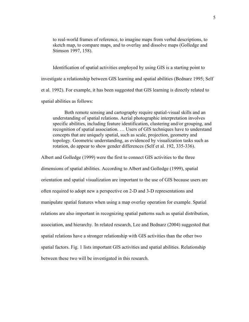
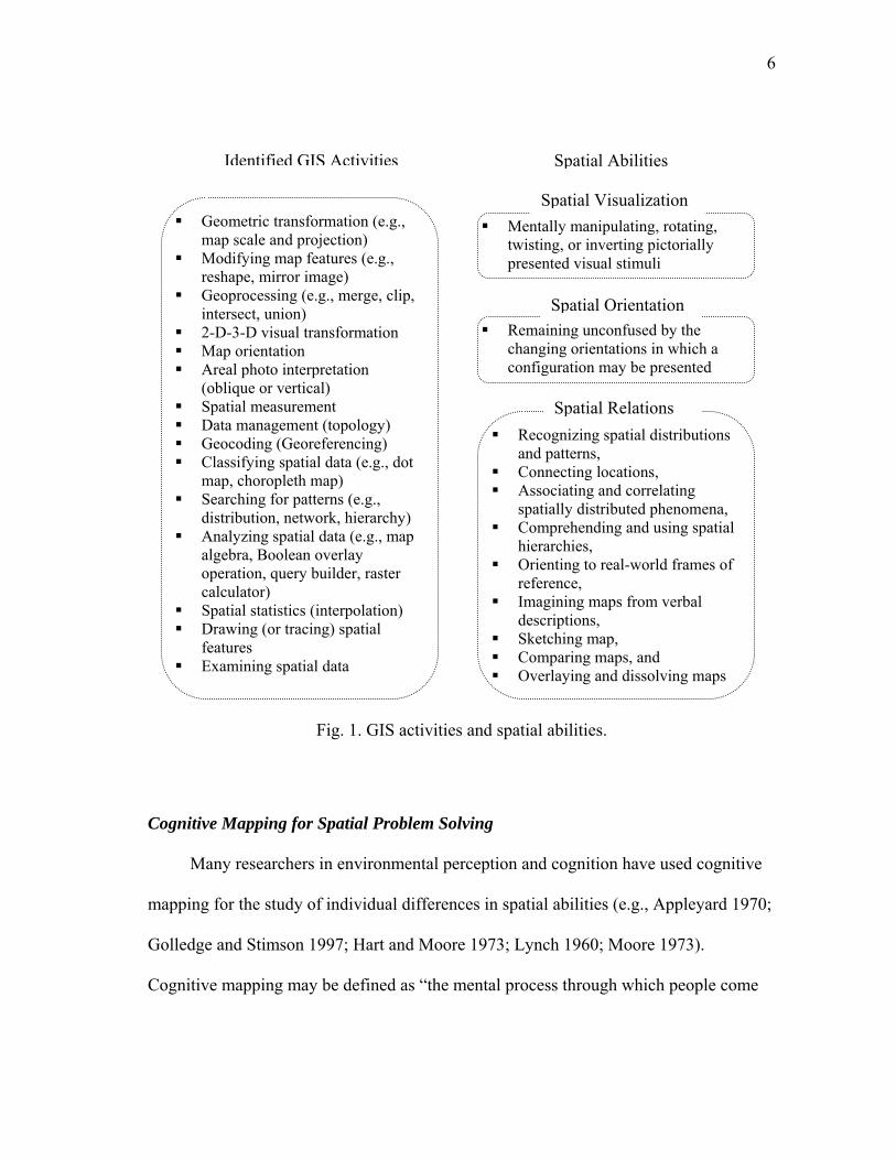
spatial factors. Fig. 1 lists important GIS activities and spatial abilities. Relationship
between these two will be investigated in this research.
6
Identified GIS Activities Spatial Abilities
Fig. 1. GIS activities and spatial abilities.
Cognitive Mapping for Spatial Problem Solving
Many researchers in environmental perception and cognition have used cognitive
mapping for the study of individual differences in spatial abilities (e.g., Appleyard 1970;
Golledge and Stimson 1997; Hart and Moore 1973; Lynch 1960; Moore 1973).
Cognitive mapping may be defined as “the mental process through which people come
Spatial Visualization Geometric transformation (e.g.,
map scale and projection) Mentally manipulating, rotating,
twisting, or inverting pictorially presented visual stimuli Modifying map features (e.g.,
reshape, mirror image) Geoprocessing (e.g., merge, clip,
intersect, union) 2-D-3-D visual transformation Map orientation Areal photo interpretation
(oblique or vertical) Spatial measurement Data management (topology) Geocoding (Georeferencing) Classifying spatial data (e.g., dot
map, choropleth map) Searching for patterns (e.g.,
distribution, network, hierarchy) Analyzing spatial data (e.g., map
algebra, Boolean overlay operation, query builder, raster calculator)
Spatial statistics (interpolation) Drawing (or tracing) spatial
features Examining spatial data
Remaining unconfused by the changing orientations in which a configuration may be presented
Spatial Orientation
Spatial Relations Recognizing spatial distributions
and patterns, Connecting locations, Associating and correlating
spatially distributed phenomena, Comprehending and using spatial
hierarchies, Orienting to real-world frames of
reference, Imagining maps from verbal
descriptions, Sketching map, Comparing maps, and Overlaying and dissolving maps

7
to grip with and comprehend the world around them” (Downs and Stea 1977, 61). When
drawing cognitive maps, people cope with spatial information, select and convert
information taken from a spatial environment into an organized representation, and
translate information from the large-scale space of world to the small-scale space of a
piece of paper (Downs and Stea 1977; Siegel 1981). The mental process used by
cognitive mappers involves spatial problem solving.
[The cognitive mapping] process generates plans for solving specific spatial problems (Downs and Stea 1977, 68).
This mapmaking requirement involves decisions about what types of
information we store, how we symbolize it, how we arrange and order it, and how we attach relative value or importance to it (Downs and Stea 1977, 77).
Additionally, cognitive mapping is a good measure of spatial ability and spatial problem
solving since cognitive mapping requires mappers to use most of the skills in the
proposed definition of spatial relations, such as recognizing spatial distributions and
patterns, connecting locations, associating spatial phenomena, comprehending spatial
hierarchies, and regionalizing.
Research Questions
It is widely recognized that spatial abilities are important in the use of GIS (Mark
et al. 1999; Montello et al. 1999). In addition, researchers have suggested that GIS
learning can positively influence the development of spatial abilities and spatial problem
solving (Albert and Golledge 1999; Audet and Abegg 1996; Audet et al. 1993; Audet
and Paris 1997; Baker 2000; Barstow 1994; Hall-Wallace and McAuliffe 2002; Keriski
2000; Salinger 1995; Self et al. 1992; Wigglesworth 2000). Empirical research, however,

8
is not sufficient to provide an understanding of where GIS learning can accomplish those
goals (Hall-Wallace and McAuliffe 2002; Kerski 2000). This study investigates the
relationship between GIS learning and spatial abilities by using a spatial skills test and a
cognitive-mapping test. This study also aims to determine how GIS learning differs by
sub-populations of students based on gender, major, and course assignment type (project
vs. paper). In order to address the central research question, operational research
questions were formulated:
1. Will GIS learning affect students’ spatial ability?
a. Will completion of a GIS course affect the spatial ability of college
students? Will completion of a cartography course be equally effective
as a GIS course?
b. Will these effects be different for male and for female students? Will
these effects differ by students’ academic majors?
c. Is there a relationship between students’ spatial abilities and learning
achievement in a GIS course?
2. Will GIS learning affect students’ spatial problem solving?
a. Will completion of a GIS course affect the map-drawing strategy of
college students?
b. Is there a relationship between students’ map-drawing strategies and
spatial ability?
9
Research Methods
Psychometric tests have been used extensively to assess spatial abilities especially
spatial visualization and spatial orientation (e.g., Goldstein et al. 1990; Kail et al. 1979;
McGlone 1981; Miller and Santoni 1986; Newcombe and Dubas 1992). “Spatial” in the
psychometric tests, however, refers only to small-scale (table-top) space which is not the
scale most relevant to geography. Furthermore, psychometric tests hardly assess the
“spatial relations” dimension which is most closely related to GIS activities (Golledge
1993; Lee and Bednarz 2004; Self et al. 1992). Since the type of standardized tests of
spatial relations that were necessary for this study did not exist, a set of new tests was
developed. Two paper and pencil tests, a spatial skills test and a cognitive-mapping test,
were designed to measure performance on a variety of spatial abilities.
The spatial skills test contained a total of 14 multiple-choice questions and
performance exercises. It was designed to evaluate students’ spatial abilities, including
overlaying and dissolving a map, reading a topographic map, finding the best location
based on several spatial factors, correlating spatially distributed phenomena,
constructing contours based on point data, and recognizing spatial data models. A total
of 80 undergraduate students at Texas A&M University completed both pre- and
posttests administered during the 2003 fall semester.
The cognitive-mapping test asked participants to draw a sketch map of a familiar
region. It was designed to identify students’ problem-solving approach, which was
measured by analysis of their map-drawing strategy. This study presumed that analysis
of individuals’ map-drawing strategies would reveal information about the cognitive

10
processes subjects used to operate in their environment. The participants were recruited
from students enrolled in a GIS and a cartography course at Texas A&M University
during the 2003 fall semester. A total of 64 students completed both pre- and posttests
administered at the beginning and end of the semester. The cognitive-mapping tests were
pilot tested twice during the 2003 spring semester. By comparing pre- and posttest maps
that the participants produced, changes in map-drawing strategies from pre- to posttest
could be determined.
Study Significance
As a result of the rapid growth of GIS industry, the importance of education and
training in GIS has never been greater (Forer and Unwin 1999; Longley et al. 1999).
Research regarding the teaching and learning of GIS places most of its emphasis on
discussing what should be taught in a GIS course or strategies for teaching particular
concepts of GIS (Bednarz 1997). The majority of this previous research fails to provide
discussion of changes in the cognitive abilities of the students. Although GIS researchers
and educators have suggested that GIS learning can contribute to the development of
spatial ability and the improvement of spatial problem solving, this claim has not been
proven experimentally (Albert and Golledge 1999). In recent years a number of articles
have been published asserting that utilizing GIS in the classroom will improve students’
spatial ability and problem-solving skills. Empirical research, however, is not enough to
understand where GIS learning can accomplish these aimed-for goals (Hall-Wallace and
McAuliffe 2002; Kerski 2000).
11
The outcome of this study provides a first step toward explaining the relationship
between GIS learning and the development of spatial abilities. There is little research
that has tested whether individuals exposed to geographic training have greater success
in understanding spatial knowledge than those who have not been exposed (Golledge
1993). Furthermore there has been little research on gender differences and GIS learning
(Self et al. 1992). GIS curriculum development would benefit from the results of this
research.
Even though psychometric tests have been widely used to measure spatial abilities,
these tests fail to assess the spatial relations dimension, which is most closely related to
GIS activities. Virtually no research has been undertaken concerning spatial relations in
the area of spatial cognition, either by geographers or psychologists (Golledge 1993).
This study provides an initial attempt to develop a paper-and-pencil test that can directly
measure some components of spatial relations.
In addition, cognitive-mapping tests provide an alternative way to measure the rich
spatial ability more related to real-world situations and problem solving. In particular,
this study attempts to identify individuals’ map-drawing strategies based on analysis of
videotapes of students’ mapping sessions and follow-up interviews conducted while
students watched video clips of themselves. Later, this study introduces specific
typologies concerning efficient strategies and common strategies that were used to
evaluate the participants’ performances (spatial problem solving).
Finally, this study sheds light on a relatively untouched issue: the relationship
between spatial aptitude and spatial-strategy selection by correlating participants’ spatial
12
ability with their strategy used in the cognitive-mapping test.
Study Assumptions
1. This study assumes that individuals’ spatial abilities can be measured and that
the spatial skills test created for this study is valid.
2. This study assumes that subjects’ mapping strategy is a valid representation of
their spatial problem-solving strategy.
3. This study assumes that differences between the pre- and posttest are results of
the treatment.
4. This study assumes that students enrolled in the GIS course achieved the
learning objectives of the course.
5. This study assumes that subjects provide answers to interview questions that
accurately represent their knowledge.
Study Limitations
1. Participants are not randomly assigned to treatment groups, thus the research
can not assume that the sample is representative of a greater population and
limits conclusions to the sample.
2. Since this study does not affect students’ grades, students may perceive it as
less relevant, and not try as hard.
3. The internal reliability of the spatial skills test is relatively low (Cronbach's
alpha = .7034).

13
CHAPTER II
REVIEW OF LITERATURE
The main focus of this study is to analyze the effect of GIS learning on students’
spatial ability and spatial problem solving. This literature review aims to provide a
background and context for this research question. It is divided into four sections.
The first section explores spatial cognitive processes of GIS activities. This
examination provides an answer to questions such as what insights GIS allows that other
ways of learning do not (Salinger 1995), and what kinds of experiences that are unique
to GIS learning. This review focuses on the analytical and visual processes of GIS. The
second section reviews spatial ability in the context of GIS. This section also discusses
limitations of traditional assessments of the individuals’ spatial ability (e.g.,
psychometric tests). The third section reviews spatial problem solving in the context of
GIS. Since students’ spatial problem-solving strategies are measured by analysis of their
map-drawing processes in a cognitive-mapping task, this section focuses on evaluation
methods of individual’s map-drawing strategies. The last section reviews relationships
between spatial ability and (spatial problem-solving) strategy choice.
Analytical and Visual Features of GIS
Analytical Processes in GIS
Researchers have argued that GIS is different from other information processing
systems because of its emphasis on spatial analysis functions (Anseline and Getis 1992;

14
Cowen 1988; Goodchild 1987; Maguire 1991). The term “spatial analysis” has assumed
various definitions over time such as “the quantitative study of phenomena that are
located in space” (Bailey and Gatrell 1995, 7), “the process to turn raw spatial data into
useful spatial information” (Longley et al. 2001, 278), and “set of analytical methods
which require access to both the attributes of the objects under study and to their
locational information” (Goodchild 1987, 68). Researchers agree, however, that spatial
data analysis plays a central role in GIS (Anselin and Getis 1992). The analytical
methods in GIS include (1) measurement, (2) spatial query, and (3) spatial statistics.
Table 1 synthesizes additional information about these three analytical methods.
The first method deals with measurement. Since all geographical entities of the world
can be clearly demarcated and positioned within some coordinate frame of reference
(Laurini and Thompson 1992), basic spatial properties such as distance, area, and slope
can be measured easily. The traditional manual measurements on paper maps are more
difficult to extract and less accurate when compared to the new options provided by
automatic measurement using GIS (Longley et al. 2001).
The second method deals with spatial queries. Transformation and optimization
are the most commonly used spatial query operations in GIS. Longley et al. (2001, 282)
defined transformation and optimization as follows:
Transformations are simple methods of spatial analysis that change datasets, combining them or comparing them to obtain a new dataset, and eventually new insights. Optimization techniques are normative in nature, designed to select ideal locations for objects given certain well-defined criteria.
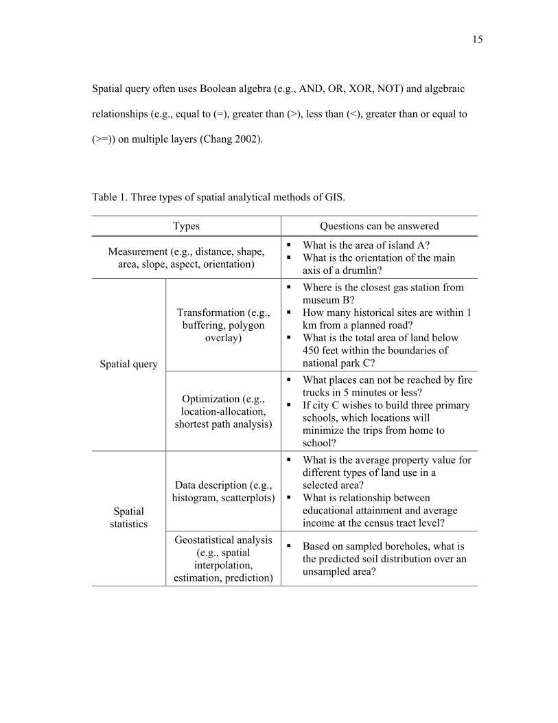
15
Spatial query often uses Boolean algebra (e.g., AND, OR, XOR, NOT) and algebraic
relationships (e.g., equal to (=), greater than (>), less than (<), greater than or equal to
(>=)) on multiple layers (Chang 2002).
Table 1. Three types of spatial analytical methods of GIS.
Types Questions can be answered
Measurement (e.g., distance, shape, area, slope, aspect, orientation)
What is the area of island A? What is the orientation of the main
axis of a drumlin?
Transformation (e.g., buffering, polygon
overlay)
Where is the closest gas station from museum B?
How many historical sites are within 1 km from a planned road?
What is the total area of land below 450 feet within the boundaries of national park C? Spatial query
Optimization (e.g., location-allocation,
shortest path analysis)
What places can not be reached by fire trucks in 5 minutes or less?
If city C wishes to build three primary schools, which locations will minimize the trips from home to school?
Data description (e.g., histogram, scatterplots)
What is the average property value for different types of land use in a selected area?
What is relationship between educational attainment and average income at the census tract level?
Spatial statistics
Geostatistical analysis (e.g., spatial interpolation,
estimation, prediction)
Based on sampled boreholes, what is the predicted soil distribution over an unsampled area?

16
The third method deals with spatial statistics. There are two types of spatial
statistics available in GIS, data description and geostatistical analysis (geostatistics).
Data description is useful for displaying the frequency or distribution of geographic data
in the form of histograms, pie charts, or scatterplots (Longley et al. 2001). Geostatistics
use statistical methods to model spatial variations in data and to predict spatial and
temporal phenomena (Krivoruchko et al. 1997; Shine and Walkfield 1999). A principal
founcation of geostatistics can be understood through Tobler (1979)’s “first law of
geography,” which states that, although all things are related, near things are more
related than distant things. The greater similarity between closer values is the basis for
interpolation methods (e.g., inverse distance weighing/IDW, kriging, polynomial
interpolation). This technique is used to estimate data for continuous variables such as
rainfall, temperature, or elevation based on a limited set of sampled figures (Longley et
al. 2001).
Hall-Wallace and McAuliffe (2002) reported that investigations with GIS improve
students’ analytical skills including data sorting, database searching, simple calculating,
and the use of statistics. Other researchers argue that GIS users must identify which
layers to include in GIS operations in order to determine spatial relationships, and this
process will improve their spatial reasoning (Barstow 1994; Thompson et al. 1997).

17
Visualization in GIS
The term “visualization” has been defined in various ways. The literature on
visualization is vast, with research emerging from multiple fields including psychology,
cognition, art, engineering, and science. MacEachren et al. (1992, 101) argues that:
Visualization… is definitely not restricted to “a method of computing,”… [It is] foremost an act of cognition, a human ability to develop mental representations that allow geographers to identify patterns and to create or impose order.
More recently, the term “visualization” has been extended to include elements of
computer imaging technology such as computer graphics, image processing, computer
vision, geometric modeling, virtual reality, and computer-aided design (Haber and
McNabb 1990; MacEachren and Ganter 1990; MacEachren et al. 1992; Visvalingam
1994).
Visualization makes scientific discovery more accessible by encoding information
in ways that facilitate the search for relevant information and rules (Cheng 1996). For
example, visualization can lead to faster and more effective problem solving by allowing
researchers to view invisible phenomena, and by displaying phenomena in different
perspectives and at different scales (Card et al. 1999; Gordin and Pea 1995; Kirby and
Pazer 1990; MacEachren et al. 1992; Petch 1994; Pinker 1984).
An ability to make visible the invisible is especially useful in solving abstract
problems (Goldstein 1996; Pinker 1984). Dynamic representations such as 3-D
visualization and virtual reality allow people to have different types of perceptual
experiences, mental instead of real, which can help them to solve problems (Höll et al.
2003). Examples of such representations could be the larger scale models of invisible

18
molecules or of DNA chains. Different representations of the same data enable people to
focus on different aspects of the problem and can enhance the understanding of spatial
data (Hall-Wallace and McAuliffe 2002; Hearnshaw 1994; Muehrcke 1990; Petch 1994).
In order to maximize the capacity of visualization as an educational tool, results from
previous research suggested that students should be provided with opportunities to
analyze, synthesize, change viewpoint and scale, and compare phenomena at multiple
perspectives (Ganter 1988; MacEachren and Ganter 1990; Medyckyj-Scott 1994;
Visvalingam 1994).
The characteristics of GIS visualization are similar to those of visualization in
general. GIS visualization serves as a tool for visual thinking and scientific inquiry by
offering dramatically different ways of looking at problems (Gordin and Pea 1995;
MacEachren et al. 1992; Medyckyj-Scott 1994). First, GIS visualization promotes spatial
analysis by presenting spatial data at different perspectives and resolutions (Andrienko
and Andrienko 1999; Barkowsky and Freksa 1997; MacEachren 1995; Monmonier
1989). “The ability selectively to emphasize features which are pertinent to a task while
suppressing less relevant information” (Medyckyj-Scott 1994, 205) allows users to
compare internal patterns which may be initially quite vague or seem independent from
or unrelated to one another (Baker 2000; Goodchild 1992; Hearnshaw 1994;
MacEachren and Ganter 1990; Medyckyj-Scott 1994; Muehrcke 1990). For example, the
interactive data classification employed by most GIS software can highlight spatial
patterns by changing the number of data classes and shifting class boundaries
(MacEachren 1995).

19
Second, GIS visualization helps users identify spatial relationships between
different spatial data by opening multiple thematic layers covering the same area
simultaneously (Barstow 1994; Hagevik 2003; Tinker 1992). For example, the display of
wildlife locations on a vegetation map may reveal the association between the wildlife
species and vegetation type (Chang 2002). Furthermore, overlayed data themes of the
same area are useful to answer “what if” questions (Ramirez 1995b).
Third, GIS visualization offers various representational formats of the same spatial
data including 2-D and 3-D maps, charts, graphs, tables, images, and animations. If they
occurred in isolation, there would be no difference between GIS visualizations and the
images produced by other information processing systems. GIS visualizations, however,
can combine graphs, charts, and tables with their display in maps. A higher level of
understanding can be acquired by examining various permutations of maps, tables, and
graphs (Egenhofer and Kuhn 1999; Muehrcke 1990; Wiegand 2003).
Finally, 3-D techniques for visualization and animation that can simulate spatial
reality allow viewers to recognize and understand spatial relationships more quickly
(Abler 1987). In GIS, for example, a 2-D isoline map can be transformed into a 3-D
image (Kavouras 1995). Now many GIS programs allow the generation of 3-D views by
draping cultural information over terrain models (Visvalingam 1994). Animation
techniques in GIS are useful to depict the sequence of events corresponding to temporal
processes such as growth and expansion (Hearnshaw 1994). Examples of animation
techniques include simulations of landslides and glacial events (GeoSolutions 2004), fire
incidents (Dodge 1996), and urban growth (Hasen 2001). In addition, animation

20
techniques can allow viewers to virtually experience environments, real or imaginary, by
using 3-D visualization techniques. For example, we can "fly" through an inaccessible
study area and look at different GIS layers draped over a digital elevation model (DEM).
In contrast to these many promising advantages of animation techniques, some
researchers suggest that animations are limited in their ability to communicate,
especially because animations are often too complex and/or too fast to be accurately
perceived and may lead readers to perceive continuous events as sequences of discrete
steps (Tversky and Morrison 2002).
Spatial Ability
This section reviews spatial ability in the context of GIS. First, this section defines
spatial abilities and discusses limitations of traditional assessments of the individuals’
spatial ability (e.g., psychometric tests). An overview of individual differences in spatial
ability follows. Finally, this review discusses how GIS learning relates to spatial ability.
This review provides a contextual background for the research questions such as how
completion of a GIS course will affect the spatial ability of college students, and how
these effects of GIS learning on spatial ability will be different for males and for females.
Definition of Spatial Ability
Cognitive psychologists, such as McGee (1979b), generally agree that spatial
ability comprises several distinct but interrelated factors. Nevertheless, some
disagreement still exists about whether there are two dominant dimensions–spatial
21
visualization and spatial orientation–or whether a third–spatial relations–is also a
fundamental dimension of spatial ability (Gilmartin and Patton 1984; Golledge and
Stimson 1997; Linn and Petersen 1985; Lohman 1979; Montello et al. 1999; Vernon
1961).
Spatial visualization refers to the ability “to mentally rotate, manipulate, and twist
two- and three-dimensional stimulus objects” (McGee 1979b, 896), or “to transform or
to recognize a transformation of one element into another; to conjure up mental imagery
and then to transform that imagery” (Gardner 1983, 176). Mentally creating a 3-D
surface from a 2-D representation is also considered spatial visualization (Gilmartin and
Patton 1984).
Spatial orientation involves “the comprehension of the arrangement of elements
within a visual stimulus pattern, the aptitude to remain unconfused by the changing
orientations in which a spatial configuration may be presented, and the ability to
determine spatial orientation with respect to one’s body” (McGee 1979b, 897). This
refers to the ability to keep a clear idea of where the individual is situated in relation to
the wider space in which he or she happens to be. Among the questions people often ask
when trying to find some orientation in space is “If the environment looks like this, what
is my position?” (Common Health of Massachusetts 2003). In geography, spatial
orientation has been used to read and analyze maps, air photographs, and digital images
(Gilmartin and Patton 1984).
Spatial relations has been suggested as a third component of spatial ability
especially by geographers (Golledge 1993). Geographers have argued that psychologists

22
have neglected some aspects of spatial phenomena such as distribution, process,
association, and structure which are important elements used in spatial activities
(Golledge 1993; Self and Gollege 1994). More specifically spatial relations refer to the
… ability to recognize spatial distributions and spatial patterns, to connect locations, to associate and correlate spatially distributed phenomena, to comprehend and use spatial hierarchies, to regionalize, to orientate to real-world frames of reference, to imagine maps from verbal descriptions, to sketch map, to compare maps, and to overlay and dissolve maps (Golledge and Stimson 1997, 158).
Few, if any, of these abilities have been tested by psychometric tests developed by
psychologists (Golledge and Stimson 1997).
Measurement of Spatial Ability
Another objection raised by geographers to psychometric tests is that the term
“spatial” in these tests refers only to small-scale (table-top) spaces (Liben 1981). Space
can be classified into two or more categories based on scale (e.g., Downs and Stea’s
small- and large-scale spaces; Ittelson’s object and large-scale spaces; Mandler’s small-,
medium-, and large-scale spaces; Montello’s figural, vista, environmental, and
geographical spaces). The most common differentiation used in published research has
been between small-scale and large-scale spaces.
Typically small-scale spaces can be apprehended from one single perspective,
from outside of the space itself (Ittleson 1973; Mandler 1983). This is the space of
pictures and small objects (Mondello 1993). The term “manipulable space” has been
used to describe this type of space, although other terms have also been suggested, such
23
as “table-top” space, “haptic” space, “sensormotor” space (Mandler 1983; Montello
1993).
Large-scale spaces, often referred to as environmental or geographic spaces, are
larger than the human body and surround it (Mandler 1983; Mark and Freundschuh
1995). The spatial relationships between elements of large-scale spaces cannot be
directly observed and must be reconstructed over time from experiences within the space
(Downs and Stea 1973; Montello 1993). Whereas small-scale space has been explored
primarily by psychologists concerned with the processes underlying environmental
cognition, large-scale space has been studied by geographers interested in answering
“what”, “where” and “why” questions in real-world situations (Spencer and Blades
1986).
Psychometric tests require individuals to find hidden shapes, match 2-D or 3-D
figures, balance figures with respect to horizontal or vertical axes, solve mazes, and
imagine the result of rotations or spatial manipulations of figures (e.g., Connor et al.
1978; Gilmartin and Patton 1984; Goldstein et al. 1990; Kail et al. 1979; McGlone 1981;
Miller and Santoni 1986; Newcombe and Dubas 1992; Tapley and Bryden 1977).
Psychometric tests, however, assess hardly any of the spatial abilities needed in real-
world problem-solving situations (Allen 1999; Freundschuh 1992; Golledge 1993;
Montello et al. 1999; Self et al. 1992). In addition, spatial relations–including spatial
correlation, association, pattern, and structure–go beyond the abilities usually evaluated
in psychometric tests (Self et al. 1992). Montello et al. (1999) and Golledge (1993)
argued that:

24
… the restricted definition of spatial ability, as incorporated into many psychometric tests, contrasts with the richness of the general literature on spatial activities and spatial behavior, much of it from disciplines other than psychology (Montello et al. 1999, 517).
[Spatial knowledge] includes higher level concepts such as hierarchy,
surface, association, connectivity, pattern, and so on. … Psychologists have neglected height or relief in their examination of spatial phenomena. In contrast, the geographer commonly represents spatial interactions, movements, or even the basic distribution or pattern of phenomena as surfaces. They are sometimes represented in two dimensional form and sometimes represented as three dimensional surfaces (Golledge 1993, 28).
Considering that GIS has been developed to deal with spatial information at the
large/geographic scale (Golledge 1993; Mark and Freundschuh 1995), psychometric
tests suffer obvious limitations for measuring the effects of GIS learning on spatial
ability (Golledge 1993). The spatial features that psychometric tests are designed to
measure are more related to jobs such as drafting, carpentry, art and design, architecture,
and sewing/clothing design than geographic problem solving (Psychological Corporation
1972).
Even though it is still a relatively unexplained field, it is important to develop new
types of assessment tools that can measure what psychometric tests cannot (Kali et al.
1997). For example, when measuring students’ spatial visualization skills acquired from
a geoscience class, Libarkin and Brick (2002, 453) noted that:
Visualization in a specific topic requires a unique set of skills; visualization of earth processes requires spatial and temporal projections not encountered in available assessment tools. Certainly, the field would benefit from instruments specifically designed for studying learning in the earth system.
Kali et al. (1997) developed a new type of test for dealing with geologic spatial ability of
college students. The test asked respondents to draw cross sections of structures

25
presented as block diagrams and to imagine block diagrams that revealed only a single
face. According to Bezzi (1991, 284):
Drawing geological maps and cross sections requires one to visualize structural shapes in the mind’s eye and to rotate, translate, and shear them. … This mental visualization … extends beyond the field of the earth sciences alone.
More recently, so-called “spatial analysis tests” were developed and applied in
geographic education by researchers such as Audet and Abegg (1996), Kerski (2000),
Meyer et al. (1999) and Olsen (2000). The spatial analysis test created by Kerski (2000)
for example, asked students to choose the best site for a fast food restaurant in a
hypothetical community based on given set of geographic (mapped) data such as traffic
volume, existing fast food locations, locations of high schools, annual median income
and zoning; students also ranked the same data according to its relative contribution to
the final selection and provided explanations to support their decisions. However, few
studies have examined the validity and reliability of this type of spatial analysis test.
Individual Differences in Spatial Ability
This section discusses whether spatial ability improves with training, and whether
training affects individuals differently depending on their gender or major. Research
concerning the impact of training on spatial ability has been inconsistent. For example,
Baenninger and Newcombe (1989), Ben-Chaim et al. (1988), Bezzi (1991), Chadwick
(1978), Kali and Orion (1996), Kali et al. (1997), Kiser (1990), Lord (1985; 1987),
Saccuzzo et al. (1996), and Smith and Schroeder (1981) reported improvement in
students’ spatial ability with training. However, studies by Mendicino (1958) and Mundy

26
(1987) found no such improvements. This inconsistency may result from the variety of
training programs and differences in spatial ability tests.
Researchers have also debated the existence and magnitude of gender differences
in the acquisition of spatial ability. While some research suggested that there is no
significant difference between men and women in spatial aptitude (Caplan et al. 1985), a
number of other studies have argued for male superiority based on various spatial ability
tests (Fennema 1975; Harris 1978; Hyde et al. 1975; Linn and Petersen 1985; Smith
1964). Better performances by men have been identified only in specific parts of spatial
skills tests, and especially in visual-spatial tasks (Chadwick 1978; Harris 1978; Kali and
Orion 1996; Liben 1981; Maccoby and Jacklin 1974; McGee 1979a; Sherman 1980).
Saccuzzo et al. (1996) also reported that men initially performed better than
women in spatial ability tests. However, after training women showed significantly
higher rates of improvement. But since men scored much closer to the maximum value
in the initial spatial ability test, women could potentially improve more after training
because their initial scores were lower (Connor et al. 1977; Goldstein and Chance 1965).
Conversely, Baenninger and Newcombe (1989) and Sorby (1998 cited in Turos and
Ervin 2000) suggested that both males and females have substantial room for
improvement in spatial ability. Research about gender differences in GIS learning still
remains insufficient and inconclusive (Baker and White 2003; Self et al. 1992).
Individual academic mastery in areas of knowledge like science has been
considered as one of the main factors that can cause differences in performance of
spatial aptitude tasks (Orin et al. 1997; Pallrand and Seeber 1984; Smith and Schroeder

27
1981). However, there has been little research on the relationship between individuals’
academic major and GIS learning. One exception is Vincent (2004), who correlated
students’ demographic information such as learning styles, spatial ability, gender, and
major to their achievement in a GIS course. His research did not find any significant
correlation between students’ academic major and performance in a GIS course.
GIS Learning and Spatial Ability
A positive relationship between GIS learning and spatial ability has been proposed
by many researchers (Albert and Golledge 1999; Self et al. 1992). Identification of
spatial activities employed by GIS users is a starting point to investigate the relationships
between GIS learning and spatial ability (Bednarz 1995; Self et al. 1992). Self et al.
(1992, 335-336), for example, suggested that:
… both remote sensing and cartography requires spatial-visual skills and an understanding of spatial relations. Aerial photographic interpretation involves specific abilities, including feature identification, clustering and/or grouping, and recognition of spatial association. … Users of GIS techniques have to understand concepts that are uniquely spatial, such as scale, projection, geometry and topology. Geometric understanding, as evidenced by visualization tasks such as rotation, do appear to show gender differences.
Albert and Golledge (1999, 10-11) were the first researchers to connect GIS activities to
the three components of spatial ability:
… it [spatial visualization] may be very important in the use of GIS. In particular, spatial visualization ability may be extremely useful in tasks such as map overlay, since map overlay involves the comparison of individual spatial elements and the performance of a logical operation on those elements, hence manipulation. Spatial visualization may also be used in the rotation and geometric transformations of 2-D and 3-D graphic representation such as map layers and DEMs…

28
… Spatial orientation may also play an important role in the use of GIS since GIS-users are often required to adopt new perspectives on 2-D and 3-D graphic representations such as a digital elevation model (DEM). In order for the GIS user to make any spatial inferences regarding shape, pattern, or layout, where the orientation of the subject is a factor, the user must adopt a new perspective, and therefore use aspects of spatial orientation….
… This ability [spatial relations] may be important in specific GIS tasks in
which mental rotation is not involved, such as the identification of features, as well as the clusters to which features belong, and the recognition of spatial association...
In related research, Lee and Bednarz (2004) also argued that the spatial relations
dimension has a more direct correlation with GIS activities than spatial visualization and
spatial orientation.
Cognitive Mapping and Problem Solving
This section reviews spatial problem solving in a context of GIS. Since students’
spatial problem-solving strategies are measured by analysis of their map-drawing
processes in a cognitive mapping task, this section focuses on methods to evaluate
cognitive maps and cognitive mapping. This section provides the background context for
the research question that investigates how completion of a GIS course will affect the
map-drawing strategy of college students.
Researchers of environmental perception and cognition have used cognitive maps
and cognitive mapping to study individual differences in spatial abilities (e.g., Appleyard
1970; Golledge and Stimson 1997; Hart and Moore 1973; Liben 1981; Lynch 1960;
Moore 1973). Cognitive mapping may be defined as “the mental process through which
people come to grip with and comprehend the world around them” (Downs and Stea
29
1977, 61). The product of this process can be considered as a cognitive map (Downs and
Stea 1973).
Different methodologies have been used to study various aspects of cognitive
maps and cognitive mapping (Anooshian and Siegel 1985). These methodologies include
(1) mechanical approaches (e.g., counting items and evaluating the accuracy of distance
estimation), (2) structural approaches (e.g., classifying maps based on the level of
cognitive development), and (3) process-oriented approaches (e.g., looking at cognitive
mapping as spatial problem solving).
Mechanical Approach
The simplest approach has been to count items in subjects’ maps. According to
Lynch (1960), cognitive maps contain five basic elements: paths, edges, nodes, districts
and landmarks. Devlin (1976), Evans et al. (1981), and McNamara et al. (1989)
tabulated the amount of spatial information, such as paths, nodes (path interactions),
labels, and landmarks, that subjects put on their maps. However, people do not always
map everything they see and remember (Foley and Cohen 1984). For example, the
importance of roads is over-estimated if one uses sketch maps to evaluate spatial
cognition as opposed to memory reports of subjects (Carr and Schissler 1969). Although
individuals cannot map features they are not aware of, they might also choose to reduce
the amount of information they map to prevent the maps from becoming cluttered or
exceedingly detailed. Other researchers have assessed maps by measuring relative

30
distance and the absolute coordinate errors (Antes et al. 1988; Briggs 1981; Brown and
Broadway 1981; Cadwallader 1979; McGuinness and Sparks 1983).
These mechanical approaches have the common assumption that the quality of
people’s cognitive maps can be measured by comparing them to accurate Euclidean
maps. Some researchers have found high correlations between perceived and actual
distances (Baird 1979; Golledge and Zannaras 1973), but others point out that cognitive
maps are always distorted with respect to Euclidean geometry, and thus the level of
distortion will likely depend on individual differences such as their age, environmental
experience, graphic skills, style of training, and patterns of thinking (Downs 1981;
Downs and Stea 1973; Golledge and Stimson 1997). Non-Euclidean information also
influences people’s selection of landmarks (Hirtle and Jonides 1985), and several studies
have shown that subjects’ familiarity with, preference for, and the function of, routes and
landmarks affect their ability to estimate distance accuracy (Antes et al. 1988; Canter
and Tagg 1975; Lee 1970). Other researchers have identified additional distance
estimation effects. For instance, Sadalla and Magel (1980) found that people consistently
judged a route containing more turns as longer than one of the same length containing
fewer turns. Sadalla and Staplin (1980) found that routes with fewer interactions were
estimated to be shorter than those with more interactions. Kosslyn et al. (1974) reported
that both preschoolers and adults overestimated the distance of a route containing a large
opaque barrier, compared to a route with no barrier. This study suggests that an adequate
model of mental mapping cannot be built around a strictly Euclidean conception.

31
Structural Approach
In contrast to mechanically analyzing the accuracy and amount of information
included in cognitive maps, the structural approach classifies cognitive maps based on
the developmental level of the spatial abilities required to draw the maps. This approach
implies that cognitive maps possess kinds of structural properties that we are familiar
with in “real” cartographic maps (Boyle and Robinson 1979). Most of this work is based
on Piaget’s extensive theorizing about spatial ontogeny, including his idea that people
progress from topological to projective and metric knowledge (Piaget and Inhelder 1967).
For example, Hart and Moore (1973) discussed three categories of reference systems–
egocentric, fixed, and coordinated–observed in cognitive maps. A few findings in the
environmental cognition literature supported the Piagetian hypothesis. For instance,
Moore (1973) had independent judges classify adults’ sketch maps based on their
developmental level. Maps judged as level I (egocentric) maps organized
undifferentiated elements from a personal perspective. These maps typically included
serpentine-like routes comprised of personally significant street segments bearing little
resemblance to the actual geographical relations between these streets. Level II (linear-
route) maps were partially coordinated and organized around one or two different
referent points. Level III (abstract coordinated) maps were characterized by features of
interest embedded in an overall geometric organization.
In related research, Appleyard (1970) found that sketch maps drawn of Cuidad
Guayana by 320 inhabitants were structured either sequentially, using roads and rivers as
organizing features, or spatially, using buildings and districts (Fig. 2). The better

32
educated residents produced spatially structured maps rather than sequential maps.
Appleyard’s conclusion that sequential maps were of a lower developmental order than
spatial maps supported the findings of Shemyakin (1962), who used the terms “route
map” and “survey map” to classify the developmental stage of representation in
cognitive maps. According to Shemyakin (1962), a route map consists of a sequence of
landmarks identifying a particular location. With more experience, information about
different routes is integrated into a network-like structure, producing a survey map.
Fig. 2. The sequential and spatial map from Applyard (1970).
Appleyard (1970) reported that differences in structuring cognitive maps were
caused more by cognitive differences, travel mode, and familiarity than by other

33
personal variables such as age, sex, and occupation. Miller and Santoni (1986) found
significant correlations between accuracy in map use and the completion of specific
courses such as math. Moore (1979) went on to argue that the overall education level
was not important in the construction of cognitive maps, but what was more important
was the development of specific cognitive abilities needed for processing spatial
information. Moore (1975a; 1975b) compared the scores in spatial skills from the
Differential Aptitude Test (DAT) with the level of cognitive mapping performance of
high school students. The results indicated that none of the verbal reasoning or
numerical ability scores was significantly correlated to the level of cognitive mapping
performance. There was, however, a highly significant and strong correlation between
spatial ability and the developmental level of students’ cognitive maps. This finding was
supported by O’Laughlin and Brubaker (1988) who reported a positive relationship
between participants’ performance on the Mental Rotation Test (MRT) and a cognitive
map task.
Process-Oriented Approach
The process-oriented approach helps us to get away from focusing on the finished
map (product), and to refocus on spatial problem solving as an intrinsic characteristic of
cognitive mapping (Downs 1981). When drawing cognitive maps, people have to deal
with spatial problems such as selecting information from their spatial environment and
converting it into organized representations, thus translating information from the large-
scale space of the real world into the small-scale space of a piece of paper (Beck and

34
Wood 1976; Downs and Stea 1977; Kuipers 1978; Siegel 1981). The following
quotations provide additional examples of problems people confront during cognitive
mapping.
In producing the street map, we have to decide upon its purpose. Who is it for: Will it be for pedestrians or drivers, for strangers to the city or current residents, for sightseeing or everyday living? The answer to this question is crucial since it determines both who the representation is useful to, and what types of spatial problem it can assist in solving (Downs and Stea 1977; 64).
[The cognitive mapping] process generates plans for solving specific spatial
problems (Downs and Stea 1977, 68). This mapmaking requirement involves decisions about what types of
information we store, how we symbolize it, how we arrange and order it, and how we attach relative value or importance to it (Downs and Stea 1977, 77).
The visual scene presents one view of the space, while the map presents an
alternative representation. In order to accurately decide which way to go, it is necessary to bring these two views of the space into correspondence. … Mental transformations may need to be done in order to coordinate these views to make accurate decision (Gunzelmann and Anderson 2002, 387).
The representation and operations upon it [cognitive map] tell us how the
person solves a problem, remembers a sentence, answers a question or makes a decision (Trabasso and Riley 1975, 381).
Since cognitive mapping and GIS use require people to rely on common mental
processes, GIS learning should affect people’s spatial ability and spatial problem solving.
Actually, Golledge (1993) suggested that cognitive mapping is like an internalized GIS
in order to emphasize the common processes employed by GIS users and cognitive
mappers.
The rapid development of GIS as a means for coding, storing, accessing, analyzing, representing and using spatial data creates an obvious parallel with the cognitive mapping process – which also encodes, stores, internally manipulates, decodes and represents spatial information. We offer a metaphor that may be useful when dealing with both concepts –i.e., that the cognitive map is an

35
internalized GIS (Golledge and Bell 1995, 1).
Another reason why cognitive mapping is a good measure of spatial ability is that
cognitive mapping requires mappers to use most of the skills in the proposed definition
of spatial relations such as recognizing spatial distributions and patterns, connecting
locations, associating spatial phenomena, comprehending spatial hierarchies, and
regionalizing. However, little is known about the relationship between specific spatial
abilities and cognitive map formation, or which abilities make the most important
contribution to cognitive map learning (Allen 1999; Kitchin and Blades 2002).
How People Draw a Map: Map-drawing Strategy
Kitchin (1997) argues that commonly used strategies employed in a cognitive-
mapping task can be identified objectively. However, there have been few attempts to
reveal which strategies are used in constructing cognitive maps (Foley and Cohen 1984).
Some possible research questions might include: “What strategies are used to construct
cognitive maps?” “How many strategies are used to construct cognitive maps?” “Do
different strategies (cognitive mapping) lead to different results (cognitive maps)?”
Although not much has been written about the process of creating cognitive maps
(Kitchin 1997), research concerning the “anchor hypothesis” (Couclelis et al. 1987;
Golledge 1978; Golledge and Zannaras 1973)” and the “rational analysis framework”
(Anderson 1990; 1991) offers a starting point.
An “anchor” is a personal, familiar landmark that serves as a reference point for a
region of space. Cognitive maps are organized according to reference points known as

36
anchors. Anchors (or reference points) are closely related to Lynch’s (1960) landmarks.
The concept of landmark has multiple referents. The term has been used to denote (a)
discriminable features along a route, that signals navigational decisions; (b)
discriminable features of a region, that allow a subject to maintain a general
geographical orientation; and (c) salient information in a memory task (Sadalla et al.
1980). Anchors tend to be large, have important functions in the environment, and be
perceived as a point feature such as a building. Nevertheless rivers and roads, classified
as paths by Lynch (1960), are able to function as anchors too. According to Ferguson
and Hegarty (1994), linear landmarks are remembered better than point landmarks
because they occupy a larger amount of space.
These anchors and the linkages between them provide a skeletal hierarchical
structure for representing and organizing cognitive information about space (Couclelis et
al. 1987). Because a reference point is regarded as a place that defines the position of
other adjacent places, it follows that other places are seen “in spatial relation to” a
reference point rather than vice versa (Rosch 1975). Researchers hypothesized that a
system having a number of reference locations from which the location of other places
could be computed would make fewer demands on an individual’s storage capacity than
would a system that tried to represent the spatial relationships between all known
locations (Sadalla et al. 1980). The relation between “anchors” and details has been
understood as function of hierarchy. A large-scale external environment such as urban
area can be conceptualized as a collection of parts. These parts consist of a set of
hierarchical nodes, hierarchical paths connecting the nodes, and areas of various scales

37
and with various degrees of generalization (Golledge 1978). The location of different
places is known with different degrees of certainty (Sadalla et al. 1980). The locations of
anchors are represented at a higher level of the hierarchical scheme whereas other
landmarks are represented at a lower level, inferred from the locations of their anchors
(Stevens and Coupe 1978).
One method for discovering the hierarchy implicit in a cognitive representation is
to examine the order in which people include landmarks when drawing their maps. If
anchors are functioning as reference points, they should be drawn before other
landmarks so that landmarks can be located with respect to anchors. By videotaping the
order in which people create a map, this assumption can be verified. In order to deduce
mappers’ spatial skills and knowledge used for their cognitive maps, one must be able to
identify the mappers’ strategy accurately. Although individuals often record the same
things on their cognitive maps, there is no evidence that they record them in the same
way (Billinghurst and Weghorst 1995; Lohman and Kyllonen 1983). As the present
study will show, it is frequently difficult to determine a mapper’s strategy solely by
examining a finished map.
While the anchor analysis theory deals with the structural process of map-drawing,
the rational analysis framework focuses on the decision-making aspects of cognitive
mapping. To solve a problem requires the determination of a sequence of decisions
(Anderson 1991). Problem solving research shows that people seldom plan complete
sequences of actions before acting (Anderson 1990; Gunzelmann and Anderson 2003).
As several authors (e.g., Anderson 1990; O’Hara and Payne 1998) have pointed out,

38
problem solvers construct partial plans, execute the action based on the partial plans, and
keep planning as they act. Therefore, every problem-solving behavior lies somewhere
along the continuum between the following two extremes:
At one extreme, a single action is decided and executed based purely on the current state of the problem. … However, this usually leads to inefficient solutions to the problem. At the other extreme of the planning continuum, a complete sequence of action is planned out before any action is executed. This results in highly efficient performance, as the best sequence of actions can be chosen and executed. However, the costs associated with planning often nullify any benefit that the planning can bring (Fu 2003, 99).
One explanation for this kind of trade-off was given by Anderson (1990) who perceived
the operation of human memory as an optimization process. In his rational analysis,
human memory maximizes the expected utility of the memory system by balancing each
cost against an expected gain.
With respect to problem solving it was assumed that the goal of the system was to achieve certain states of affairs (e.g., getting from one location to another). Achieving a state of affairs has some value, G. The problem solver is characterized as searching for some plan which will achieve this state of affairs. Any plan is characterized as having a certain cost, C, and probability of success, P. The rational behavior is one of choosing among plans to find one that maximizes PG – C and executing it, provided its expected value is positive (Anderson 1991, 481).
Thus, under the rational framework, the planning process should stop as soon as the cost
of further planning exceeds the benefit that further planning could bring (Christensen-
Szalanski 1980). The idea is that continued search for answers to the problem takes place
at increasing costs. That is, a problem solver reaches temporary satisfaction by selecting
the best plan at the time, without any guarantee that it will be the best overall option.
In order to understand the problem-solving process in cognitive mapping, it is not
sufficient to consider just the internal representation of the task and how this task is
39
processed. For example, the interleaving of planning (internal representation) and action
(drawing) allows for additional reactive and opportunistic planning actions (O’Hara and
Payne 1998). Additionally, implementing representation tools in the planning process
reduces both uncertainty in the problem-solving process and the load on working
memory (Anderson 1991; Kirsh and Maglio 1994).
In summary, some people solve spatial problems based on more developed long-
range plans, while others solve spatial problems based on short-range plans. For example,
when people attempt to find the shortest route from location A to location B, they have
to consider several spatial variables such as traveling time, distance, road conditions,
traffic signs, speed limits, construction sites, etc. People who consider several variables
simultaneously and plan further will likely produce more efficient solutions to their
problems when compared to people who consider fewer variables. However, individuals
cannot hold a long sequence of actions in their minds due to the limits of their memory
(Anderson 1991). Thus, more plan-based strategies require greater cognitive efforts that
often result in additional time costs.
Since strategies that are based on short-range plans require less cognitive effort,
these strategies allow for quicker responses to changing external conditions. However,
strategies using short-range plans often lead to limited solutions that require more trial
and error sequences in order to reach the same goal, often resulting in less efficient
solutions to the problem (Fu 2003; O’Hara and Payne 1998).

40
Relationship between Aptitude and Strategy Choice
This review provides a framework and rationale to understand the research
questions such as whether there is a relationship between students’ map-drawing
strategies and spatial ability. This section reviews relationships between spatial ability
and (spatial problem-solving) strategy choice. An overview of the major research
findings concerning the effects of spatial aptitude on spatial task performance follows.
Researchers agree that different people do employ different strategies when
solving the same spatial tasks (Anzai and Simon 1979; Kyllonen et al. 1984a, 1984b;
Lohman and Kyllonen 1983). It is quite unclear, however, how these different spatial
strategies come about. They may be caused by variations in cognitive styles, or they may
be due to individual differences in spatial ability. Therefore, it is fundamental to study
the relationship between individual aptitude and strategy choice.
Is there a relationship between aptitude and strategy? Kyllonen et al. (1984a) and
Lohman and Kyllonen (1983) identified three possible types of aptitude-strategy
relations. In the first case strategy selection is limited by aptitude, because the use of a
strategy requires particular skills. Differences in how subjects solve problems are
entirely a function of differences in aptitude. Consequently, the strategy is the aptitude
(Lohman and Kyllonen 1983). In the second case strategy choice is not related to
aptitude; the effectiveness in solving tasks depends on the aptitudes required by each
strategy. In this case, strategy is important for understanding task performance, but
irrelevant for understanding aptitude (Lohman and Kyllonen 1983). In the third case the
relationship between aptitude and strategy combines the first two types of aptitude-

41
strategy relations: Aptitude limits both strategic choices and effectiveness in the use of
the selected strategy.
There is evidence that subjects’ ability plays a role in their strategy choices and
efficiency (Freedman and Rovegno 1981; Lohman and Kyllonen 1983; Kyllonen et al
1984a; 1984b; Schultz 1991; Snow 1980). For example, Freedman and Rovegno (1981)
investigated strategies for a mental rotation test using a retrospective questionnaire. They
reported that high-ability individuals, males, and right-handed individuals tend to use
more nonverbal, holistic strategies than their counterparts. In related research, Kali et al.
(1979) examined gender differences on a mental rotation task and concluded that some
subjects rotated an image holistically, while others compared selected features
sequentially and analytically; female participants used the latter strategy more often.
In theory, subjects who use holistic strategies take longer to solve problems, since
they must perform mental manipulations of the figures. In contrast, subjects using
analytic strategy select a feature on the target figures and check it against the response
figure, alternating looks at the target and response figures (Bruin et al. 2000). Snow
(1978; 1980) found that high-ability subjects tend to choose more constructive matching
strategies, whereas low-ability subjects choose more response-elimination strategies.
Other studies did not find these types of relationships between aptitude, strategy
choice, and performance (e.g., Bruin et al. 2000; Latwon 1994; O’Laughlin and
Brubaker 1988). For instance, Latwon (1994) found no relationship between mental
rotation ability and way-finding strategy, which is a behavior dependent upon the
process of cognitive mapping (O’Laughlin and Brubaker 1998). In examining strategic
42
and gender differences in solving a spatial visualization task, Bruin et al. (2000) reported
that strategy choice was not related to aptitude level or gender. Tapley and Bryden
(1977) concluded that strategy was not related to performance accuracy either for real
object or mental rotation tasks.
In summary, existing research on this topic is still insufficient and inconclusive to
determine the relationship between aptitude and strategy choice (Bruin et al. 2000).
Furthermore, there is little research concerning different map-drawing strategies in a
context of spatial aptitude. However, it is clear that individual differences in spatial
strategy are relevant to spatial performance. A better understanding of strategy choice
and its relationship to spatial performances will be an important further for the
understanding of variations in spatial ability (Schultz 1991).
Summary
The purpose of this literature review was to provide background and context for
research questions concerning the effect of GIS learning on spatial ability and spatial
problem solving. The most relevant research performed in this field is summarized as
follows.
GIS is different from other information processing systems due to its emphasis on
spatial analysis and spatial visualization functions (Anseline and Getis 1992; Cowen
1988; Goodchild 1987; Maguire 1991). GIS analytical methods including spatial
measurements, calculations, spatial queries, and spatial statistics can improve students’
analytical skills and spatial reasoning (Hall- Barstow 1994; Thompson et al. 1997;

43
Wallace and McAuliffe 2002). GIS visualization serves as a tool for visual thinking and
scientific inquiry by offering dramatically different ways of looking at problems (Gordin
and Pea 1995; MacEachren et al. 1992; Medyckyj-Scott 1994).
Definitions of spatial abilities are tied to performance on spatial aptitude tests and
to the dimensions of visualization and orientation contained within those tests (Golledge
and Stimson 1997). Golledeg (1993) also suggested that spatial relations is the third
dimension of spatial ability, and it includes characteristics such as spatial correlation,
association, pattern, and structure. Although psychometric tests have been widely used
to measure spatial ability, they have limitations to assess spatial relations, which is the
element most closely related to GIS activities. More recently so-called “spatial analysis
tests” were developed to measure participants’ spatial problem solving in geographic
educational research (e.g., Audet and Abegg 1996; Kerski 2000; Meyer et al. 1999;
Olsen 2000). However, few studies have examined the validity and reliability of this
type of spatial analysis test.
Since cognitive mapping and GIS use make people rely on common mental
processes, GIS learning should affect people’s spatial problem solving. For example,
when drawing cognitive maps, people have to deal with spatial problems such as
selecting information from their spatial environment and converting it into organized
representations, thus translating information from the large-scale space of the real world
into the small-scale space of a piece of paper (Beck and Wood 1976; Downs and Stea
1977; Kuipers 1978; Siegel 1981). Analyzing videotaped map-drawing processes can
provide more information than the analysis of finished paper maps. Although not much

44
has been written about the process of creating cognitive maps (Kitchin 1997), research
concerning the “anchor hypothesis” (Couclelis et al. 1987; Golledge 1978; Golledge and
Zannaras 1973)” and the “rational analysis framework” (Anderson 1990; 1991) offers a
starting point.
Researchers agree that different people employ different strategies when solving
the same spatial tasks (Anzai and Simon 1979; Kyllonen et al. 1984a, 1984b; Lohman
and Kyllonen 1983). It is quite unclear, however, how these different spatial strategies
come about. It has been suggested that the subjects’ abilities play a role in their strategy
choices and efficiency (Freedman and Rovegno 1981; Lohman and Kyllonen 1983;
Kyllonen et al. 1984a, 1984b; Schultz 1991; Snow 1980). The same principle can be
applied to understand the relationships between spatial ability and a choice of cognitive-
mapping strategy.

45
CHAPTER III
RESEARCH METHODOLOGY
Two research assessments were conducted to measure changes in spatial ability
and spatial problem solving of students, before and after they completed a GIS course.
This chapter describes the research design and methods involved in these two
assessments: a spatial skills test and a cognitive-mapping test.
Experiment 1: Spatial Skills Test
Experiment #1 was devised to determine whether the completion of a GIS course
changed the spatial ability of college students. In order to address this issue
comprehensively, the experiment considered a series of related factors such as whether
students with different gender or academic major perform in a comparable way after
completion of a GIS course, whether the completion of a computer cartography course
was equally effective as the completion of a GIS course for the improvement of spatial
ability, and whether there was a relationship between students’ scores on the spatial
skills test and their performance in a GIS course.
Test Descriptions
Spatial relations is the dimension of spatial ability that has the closest correlation
with GIS activities. It has a stronger correlation with GIS than either spatial visualization
or spatial orientation, two other spatial dimensions that have been frequently used in
46
psychological research (Lee and Bednarz, 2004). However, because there are no
standardized tests dealing with the spatial relations dimension, a new test was developed
for this study. The development of this spatial skills test followed these steps: (1)
identification of the test purpose and specification of concepts measured, (2)
construction of the initial pool of items, (3) pilot testing, (4) item analysis, and (5) field
testing.
The initial step in the construction of a test is the delineation of the assessment
objective. This process includes a description of the test content and constructs to be
measured (Plake and Jones 2002). A careful specification of the test content also helps to
improve its content validity. The spatial relations defined by Golledge and Stimson
(1997) provided a guideline for developing test contents. Each test item was designed to
measure a component or a trait of spatial relations as defined by Golledge and Stimson
(1997). The spatial skills test consists of a set of multiple-choice questions and
performance exercises (APPENDIX 1).
The final version of the spatial skills test includes seven types of question items:
(1) overlaying and dissolving a map, (2) choosing the best location based on several
spatial factors, (3) orienting to a real world frame of reference, (4) imagining maps from
verbal descriptions, (5) correlating spatially distributed phenomena, (6) constructing
contours based on point data, and (7) recognizing spatial data types (e.g., point, line, or
polygon). The following is a description of the item types in the study, including how
each one is related to GIS activities, and which traits each item aims to measure.
Item #1 required the participants to visually verify a map overlay process and then

47
select the appropriate map layers involved in the overlay. The map overlay operation
was selected because it is a fundamental GIS operation which requires spatial cognitive
abilities to mentally visualize and manipulate spatial objects (Albert and Golledge 1999).
Item #2 required participants to select an ideal location for a store based on
multiple pieces of spatial information such as population density and distance from
already existing stores. The basic rationale behind items #1 and #2 is to assess Boolean
logic, frequently used in GIS spatial analysis. In contrast to item #1, which involves
abstract problem solving, item #2 emphasizes situational problem solving. Both items
#1and #2 correspond to the trait “overlaying and dissolving maps” in the spatial relations
discussed by Golledge and Stimson (1997).
In item #3, participants were asked to mentally visualize real-world topography
based on the observation of a topographic map. Many modern GIS programs allow for
the generation of 3-D views by draping corresponding cultural information over terrain
models or surfaces (Visvalingam 1994). This item was necessary since participants,
while generating 3-D images based on 2-D information, may perform several cognitive
tasks including 2-D to 3-D conversion and spatial orientation in real-world situations.
This item assesses the trait of “orienting to real-world frames of reference” referred to by
Golledge and Stimson (1997).
In item #4, participants were required to locate specific places on a grid map based
only on the analysis of verbal descriptions. In order to accurately complete this test item,
the students had to critically interpret and synthesize two different types of visual
information (a grid map and a selected topographic profile) and a verbal description.
48
This item measures the trait “imagining maps from verbal descriptions” mentioned by
Golledge and Stimson (1997).
Item #5 asked participants to identify spatial correlations between sets of maps.
GIS users are frequently required to compare several layers of spatial information
pertaining to the same area in the screen. They may have to perform spatial cognitive
processes, such as “comparing, associating and correlating spatially distributed
phenomena,” and “recognizing spatial distributions and spatial patterns” (Golledge and
Stimson 1997).
Item #6 required the participants to create a contour map by connecting points
having the same elevation. In order to complete a contour map, students had to estimate
the elevation of places having no labeled data points. Even though GIS can perform
automated interpolations, students may be required to understand the process. This item
evaluates the trait “associating and estimating spatially distributed phenomena”
discussed by Golledge and Stimson (1997).
Finally item #7 asked participants to visually extract types of spatial data from
visually or verbally expressed spatial information. The recognition of spatial data types
(e.g., point, line, or polygon) is important for GIS users, especially for GIS data
management or spatial analysis. In solving this problem, participants dealt with several
cognitive traits including “imagining maps from verbal descriptions,” and “recognizing
spatial patterns” also discussed by Golledge and Stimson (1997).
Administering a pilot test to a representative sample of the population is an
important element in test preparation (Plake and Jones 2002). In this study, once a test

49
with 25 test items was developed, a pilot test was administered at the end of the 2003
spring semester. A total of 86 subjects (49 males and 37 females) took part in the test.
All subjects were classified as undergraduate or graduate students at Texas A&M
University. They were recruited from several geography courses including Computer
Cartography, Introduction to GIS, Advanced GIS, and Economic Geography. Each
received $5 for his or her participation.
Performance on the pilot test was measured based on the total number of questions
correctly answered. Item analyses were conducted for each question to evaluate clarity,
reliability, content validity, discrimination ability, and difficulty level. Items that were
too difficult, too easy, or unclear were eliminated or revised. By comparing the scores
between a control group (non-GIS users) and experimental groups (GIS users) and by
calculating the correlation between the number of GIS coursework hours finished by
GIS users and their scores on the test, it was possible to determine the correlation
between GIS learning experience and spatial abilities. The average scores of the control
group, those with no GIS experience, were compared to three experimental groups who
had completed (1) a cartography course only, (2) a GIS course only, or (3) more than
two GIS courses (Table 2). Preliminary results suggested that the average scores of all
three experimental groups were higher than the control group’s (p = 0.00). A positive
correlation existed between the number of GIS courses completed by the subjects and
their scores on the spatial skills test (Pearson correlation coefficient = .578) (Fig. 3).
Since a pretest was not administered, it was not possible to determine whether spatial
abilities were improved by completing GIS courses. After the pilot test, 17 test items

50
were selected for field testing.
Table 2. Average scores and standard deviations in the pilot test.
No GIS experience
Cartography only GIS only More than 2
GIS courses Average
Average 15.59 24.25 23.49 27.31 22.67 N 23 18 19 26
S.D. 5.86 3.59 7.13 5.79 7.27
Fig. 3. Number of GIS courses completed by the subjects and their average scores in the spatial skills test.
Subjects and Test Setting
Participants for field tests were recruited from students enrolled in Computer

51
Cartography, Introduction to GIS, and Economic Geography in the Department of
Geography at Texas A&M University during the 2003 fall semester. A total of 80
students completed both pre- and posttests at the beginning and end of the semester.
During this semester, 17 and 18 students took Introduction to GIS and Computer
Cartography respectively. Seven of the students enrolled in the Introduction to GIS
course had already finished the Computer Cartography course before the pretest was
administered. In addition, three students took both courses concurrently. Including
Computer Cartography students in the experiment provided an opportunity to compare
the effect on spatial ability of the completion of a GIS course with that of a cartography
course (Table 3).
Table 3. Control group and three experimental groups.
Group Group description
Control group (N=35) Students who have not taken a GIS or cartography course.
Cartography (N=18) Students who completed only a cartography course.
GIS (N=17) Students who completed only an introductory GIS course. Experimental
group GIS and Cartography
(N=10)
Students who completed both a cartography and an introductory GIS course consecutively or concurrently.
Introduction to GIS consisted of two lectures and one lab per week. While lectures
emphasized the underlying principles of GIS and its basic concepts of design, planning,
and implementation, the laboratory component provided hands-on experience with GIS

52
software frequently used in the real-world GIS community, namely ESRI ArcView,
Arc/Info, and ArcGIS. Lab exercises included topics such as basic GIS data models; GIS
data input, storage, and editing; elementary spatial measurement; analysis of spatial
arrangements; overlay analysis; cartographic visualization; and GIS modeling. By the
end of the semester, students were expected to complete either a GIS project or a paper
as the final assignment. Final grades were assigned based on student performance on two
exams, the lab exercises, and the final project or paper.
The Computer Cartography course was a combination of traditional cartography
and GIS. This course also combined lectures with laboratory exercises. Lectures covered
basic cartographic concepts and design principles, while laboratory exercises provided
students with hands-on experiences of map design and production in ArcView and MS
Office. Among the types of maps studied in the course were choropleth maps, dot maps,
proportional circle maps, flow maps, and cartograms.
The purpose of the course on Economic Geography was to acquaint students with
the basic principles of economics within a spatial context. The course explored topics
such as the process of globalization, technological development, the dynamic
relationship between the market and the state, and the role of transnational corporations.
Economic Geography was primarily a lecture-based course.
Since random assignment of subjects to the control and experimental groups was
not possible, a quasi-experimental method was used to measure the effect of the
independent variable (completion of GIS course or cartography course) on the dependent
variable (scores on the spatial skills test). This quasi-experimental method is the most
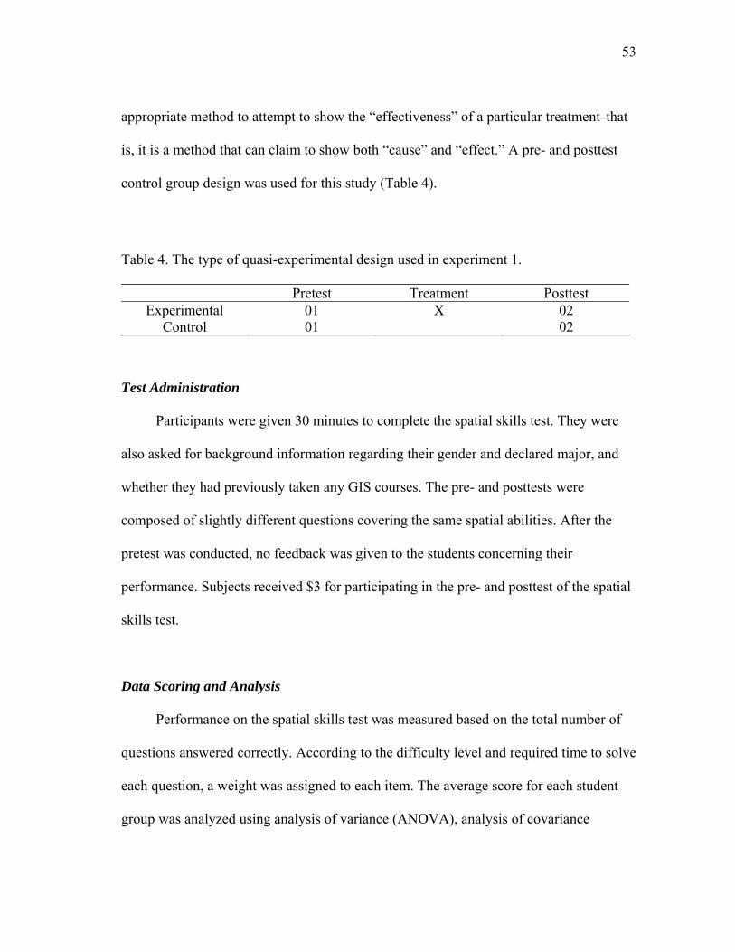
53
appropriate method to attempt to show the “effectiveness” of a particular treatment–that
is, it is a method that can claim to show both “cause” and “effect.” A pre- and posttest
control group design was used for this study (Table 4).
Table 4. The type of quasi-experimental design used in experiment 1.
Pretest Treatment Posttest Experimental 01 X 02
Control 01 02
Test Administration
Participants were given 30 minutes to complete the spatial skills test. They were
also asked for background information regarding their gender and declared major, and
whether they had previously taken any GIS courses. The pre- and posttests were
composed of slightly different questions covering the same spatial abilities. After the
pretest was conducted, no feedback was given to the students concerning their
performance. Subjects received $3 for participating in the pre- and posttest of the spatial
skills test.
Data Scoring and Analysis
Performance on the spatial skills test was measured based on the total number of
questions answered correctly. According to the difficulty level and required time to solve
each question, a weight was assigned to each item. The average score for each student
group was analyzed using analysis of variance (ANOVA), analysis of covariance

54
(ANCOVA), and a paired sample t-test. An alpha level of .05 was used to determine
whether there was significant difference between or among groups. If a significant
difference among groups occurred, post hoc comparison (using Tukey and Bonferroni
tests) was used to identify where differences had occurred.
In addition, personal interviews with the subjects who completed the GIS course
were conducted to gather information about the learning process they perceived had
occurred during the GIS course. Interview questions asked for a general evaluation of
the teaching style (lecture vs. lab) and about the advantage of completing a final project
in the course.
Experiment 2: Cognitive-Mapping Test
Research Questions
Experiment #2 was created to determine if GIS learning led to changes in the
students’ problem-solving strategies. These changes were measured by observing and
analyzing the participants’ map-drawing strategies. A previously administered pilot test
revealed that hierarchical, regional, and mixed map-drawing strategies were the three
types used by students. Comparisons of students’ map-drawing strategies were made
before and after they completed their GIS learning experience. In addition, the
correlation between each map-drawing strategy and the corresponding average scores in
the spatial skills test was also calculated.
55
Subjects
The participants were recruited from the students enrolled in the Introduction to
GIS and Computer Cartography courses at Texas A&M University during the 2003 fall
semester. A total of 64 students completed both pre- and posttests administered at the
beginning and end of the semester. Of the 64 subjects, about half (36 of 64) were
geography majors. Subjects received $3 for participating in both the pre- and posttest.
Test Descriptions and Procedure
The participants were asked to draw a sketch map of a familiar region based on the
instructions that follow (Fig. 4). Map-drawing scenario was developed by the researcher
(APPENDIX 2).
Map-drawing scenario: A friend of yours is coming to visit you here. You are unable to show your friend around. Draw a map to help your friend find some useful places in town. This map should include the O&M building (location of the Dept. of Geography), Best Buy (a large electronics store), HEB (a grocery store), and Hollywood 16 (movie theater).

56
Fig. 4. Reference map.
For the posttest, the participants were asked to locate three different commercial
locations (e.g., Barns & Noble, Target, and Sam’s Club). By selecting three different
places located near the three places used on the pretest, the pre- and posttest should be
able to maintain consistency. The target area for the cognitive-mapping task is a part of
College Station where the Texas A&M University campus is located. Two main roads,
Texas Avenue and Highway 6, traverse the target area. All four of the locations subjects
were asked to map are situated within 2 miles of the campus and are businesses
frequented by almost all students.
Each student was given an 8.5 by 11 inch sheet of white paper. Subjects were
given as long as necessary to complete their maps. Most of the subjects completed their
maps within 10 minutes. The map-drawing process of each subject was videotaped in
order to identify the subject’s map organization method. The subjects were also asked

57
how long they had lived in College Station; their usual mode of transportation; and their
declared major, age, gender, and year in school (freshman, sophomore, etc.).
After the posttest of the cognitive-mapping task, interviews with 30 subjects were
conducted in order to develop a richer understating of their map-drawing strategies. The
students’ videotapes were used to help the subjects recall their drawing experience. The
interviewer asked subjects about their map-drawing strategies, the order in which they
constructed the map, the location of their viewpoint (i.e., their orientation), and their
familiarity with the area. The interview began by asking students to describe their
mapping strategies as they watched the video tapes of themselves. After students
described the mapping procedure in their own words, they were asked to answer specific
questions such as “Why did you start with Highway 6 (a main road)?”, “How did you
orientate yourself?”, “Where was your viewpoint?”, “Why did you begin with upper-left
(or upper right) corner of a paper?”, “Why did you use a double line (or single line) for
road construction?”, and “Are you familiar with the mapping area?” Each interview was
tape-recorded and transcribed.
Pilot Tests
Pre- and posttest versions of the cognitive-mapping test were administered as part
of a pilot study in the 2003 spring semester. The participants (N=8) were undergraduate
students registered in Computer Cartography at Texas A&M University. Through the
analysis of the pilot test results, three map-drawing strategies were identified:
hierarchical, regional, or mixed. Only minor changes in map-drawing strategies were

58
found from pre- to posttest. The findings were, however, restricted due to the relatively
small sample size.
Analysis
The respondents’ map-drawing strategies were classified as hierarchical, regional,
or mixed based on the recorded data. The average time used for each map-drawing
strategy was calculated. By comparing the subjects’ map-drawing strategies in the pre-
and posttest, changes in map-drawing strategies after the completion of a GIS or
cartography course were identified. The correlation between each map-drawing strategy
and its corresponding average scores on the spatial skills test was determined. However,
no attempt was made to measure the relationship between the complexity of maps and
the average time used for drawing them.
59
CHAPTER IV
FINDINGS AND ANALYSIS
This chapter examines the statistical and qualitative outcome of the two research
experiments described in Chapter III. The results are presented in the same order as the
research experiments. Experiment #1 dealt with the spatial skills test. First, analyses of
the participants’ scores in the test were conducted to determine whether any differences
existed between the control and experimental groups. Second, the effects of the variables
related to the subjects’ background, such as gender and major, were examined. Lastly,
the correlation between the participants’ average scores on the spatial skills test and
performance in the GIS course were analyzed.
Experiment #2 involved the cognitive-mapping test. First, participants’ map-
drawing strategies were classified into three strategies (hierarchical, regional, and
mixed) and any changes in their map-drawing strategies from pre- to posttest were
determined. Qualitative data collected during interviews with subjects is reported in this
section. Second, demographic information about the participants was correlated with the
three map-drawing strategies. Lastly, participants’ map-drawing strategies were
correlated to their average scores in the spatial skills tests.
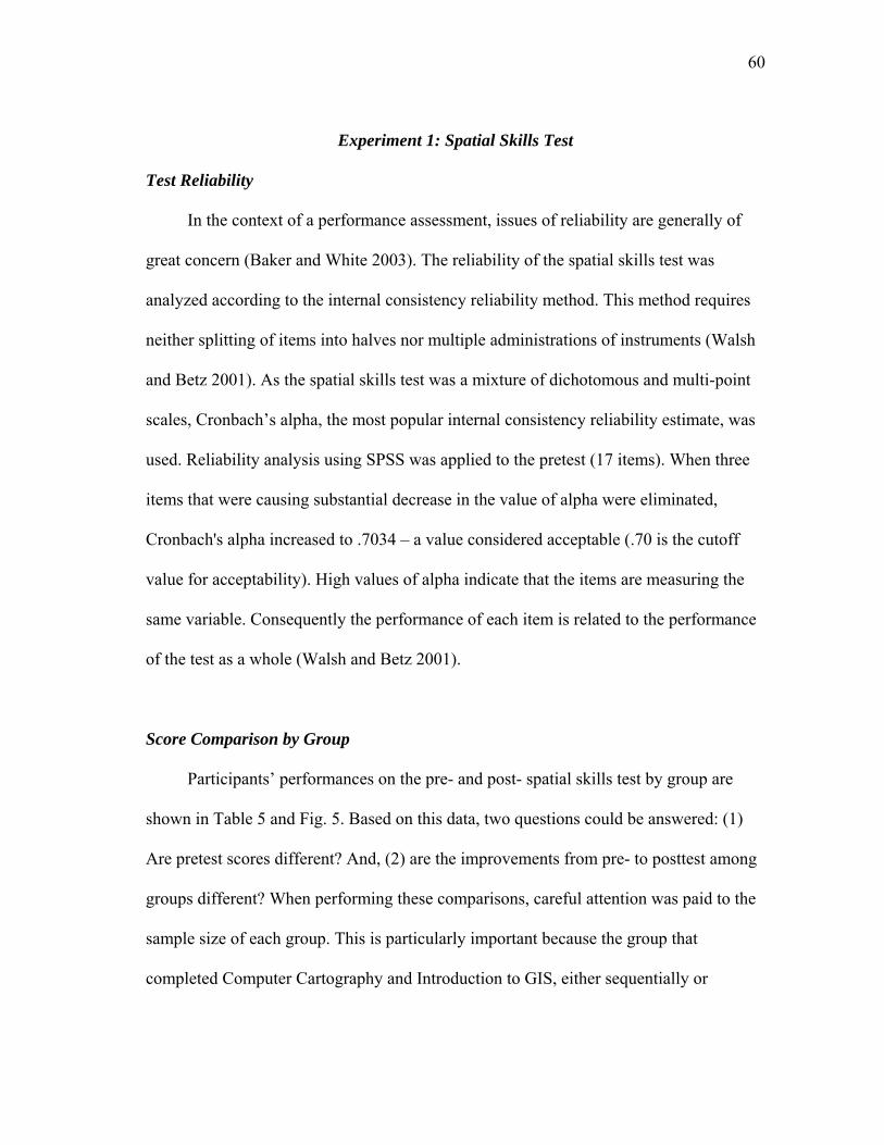
60
Experiment 1: Spatial Skills Test
Test Reliability
In the context of a performance assessment, issues of reliability are generally of
great concern (Baker and White 2003). The reliability of the spatial skills test was
analyzed according to the internal consistency reliability method. This method requires
neither splitting of items into halves nor multiple administrations of instruments (Walsh
and Betz 2001). As the spatial skills test was a mixture of dichotomous and multi-point
scales, Cronbach’s alpha, the most popular internal consistency reliability estimate, was
used. Reliability analysis using SPSS was applied to the pretest (17 items). When three
items that were causing substantial decrease in the value of alpha were eliminated,
Cronbach's alpha increased to .7034 – a value considered acceptable (.70 is the cutoff
value for acceptability). High values of alpha indicate that the items are measuring the
same variable. Consequently the performance of each item is related to the performance
of the test as a whole (Walsh and Betz 2001).
Score Comparison by Group
Participants’ performances on the pre- and post- spatial skills test by group are
shown in Table 5 and Fig. 5. Based on this data, two questions could be answered: (1)
Are pretest scores different? And, (2) are the improvements from pre- to posttest among
groups different? When performing these comparisons, careful attention was paid to the
sample size of each group. This is particularly important because the group that
completed Computer Cartography and Introduction to GIS, either sequentially or
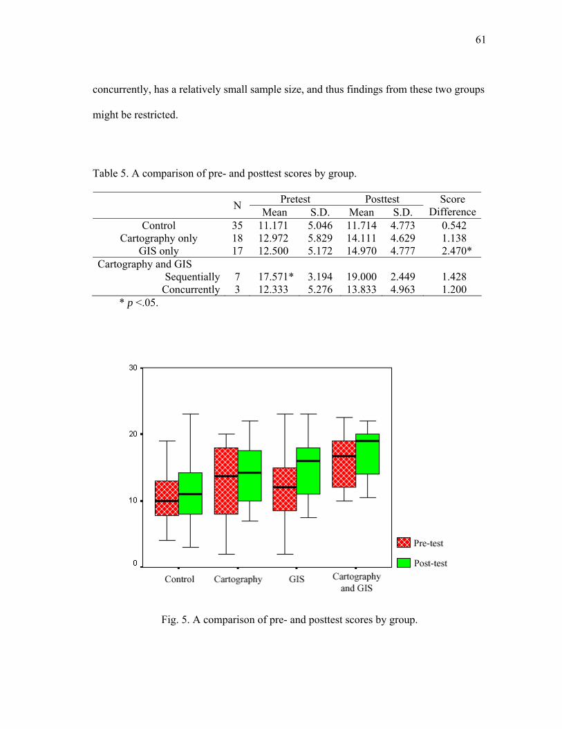
61
concurrently, has a relatively small sample size, and thus findings from these two groups
might be restricted.
Table 5. A comparison of pre- and posttest scores by group.
Pretest Posttest N Mean S.D. Mean S.D. Score
DifferenceControl 35 11.171 5.046 11.714 4.773 0.542
Cartography only 18 12.972 5.829 14.111 4.629 1.138 GIS only 17 12.500 5.172 14.970 4.777 2.470*
Cartography and GIS Sequentially 7 17.571* 3.194 19.000 2.449 1.428
Concurrently 3 12.333 5.276 13.833 4.963 1.200 * p <.05.
Fig. 5. A comparison of pre- and posttest scores by group.

62
By comparing pretest scores between groups, this study was able to determine
students’ spatial abilities prior to the treatment (GIS learning). When applying analysis
of variance (ANOVA) to the pretest scores of the four groups (excluding the group that
had only three subjects) significant differences were found (p = .032) (Table 6). A post-
hoc comparison (using Tukey method) was used to determine which groups were
significantly different from the control group and which were not. Post-hoc comparisons
indicated that students who completed the cartography and GIS courses sequentially
scored significantly higher than students of the control group (p = .019). This result
should not be surprising because these students were the only group exposed to
Computer Cartography prior to the treatment. No other significant differences between
these groups were found.
Table 6. ANOVA for pretest scores by group.
SS df MSE F p Between groups 245.747 3 81.916 3.094 .032 Within groups 1932.922 73 26.478
Total 2178.669 76
All groups changed their scores during the experimental period. Analysis of
covariance (ANCOVA) was used to determine whether there were significant
differences in score improvements between groups (Table 7). ANCOVA was applied to
the posttest scores of the four different groups, using their pretest scores as covariate to
account for initial differences in spatial abilities. After performing ANCOVA, the most
significant effects were further analyzed by post hoc comparisons in order to identify

63
differences between groups. The F statistic value of 3.697 (p = .016) showed that a
significant difference existed between the posttest scores. The post-hoc comparison
(using Bonferroni method) revealed that students that completed only the GIS course
improved their scores far more than the control group students (p = .016). This finding
indicated that completion of a GIS course is relevant for improving students’ spatial
abilities. No significant difference, however, was found between the cartography group
and the control group (p = .992).
Table 7. ANCOVA using posttest scores as the dependent variable with the pretest scores as the covariate.
SS df MSE F p Between groups 74.954 3 24.985 3.697 .016 Within groups 486.629 72 6.759
Total 1905.130 76
A t-test comparing paired sample scores between pre- and posttest within a group
produced comparable results (Table 8). The students who completed only the GIS course
increased their scores significantly as a result of the treatment (p = .002). Even though
students who completed the cartography course only and both courses sequentially had
higher scores on the posttests, their increases were not statistically significant (p = .153
and p = .180 respectively). It should be noted that students who completed both courses
sequentially were closer to the maximum potential on the pretest. Consequently, it was
more difficult for them to increase their scores on the posttest. The maximum score for
both pre- and posttest was 24.
64
Table 8. Paired sample t-test for gain scores.
Group Mean (posttest – pretest) S.D. S.E. t p
Control 0.5429 2.893 0.489 1.110 .275 Cartography only 1.1389 3.225 0.760 1.498 .153
GIS only 2.4706 2.741 0.664 3.716 .002 Carto. and GIS
sequentially 1.4286 2.490 0.941 1.518 .180
In order to determine whether some items had a larger impact than others on the
average difference between the control (N=35) and GIS group (N=27), the average
scores between the two groups were compared item by item. A total of 14 question items
were grouped into seven item types. Average scores for each group of students,
displayed by item type are shown in Table 9. Significant differences in score changes
across the item types were reported by ANCOVA statistics. Note that GIS users
increased their scores more than the control group students on item types #2, #5, and #7
(Table 9). From this one can conclude that completion of a GIS course helps students in
(1) finding the best location under various spatial conditions, (2) connecting regions
having spatial correlations, and (3) identifying spatial information as point, line, or
polygon.
Score increases from pre- to posttest in the control group in some item types (e.g.,
#1, #6, and #7) might have been caused by two major factors. First, it was not known to
what extent having previously taken a similar test may have influenced a person’s
performance of the retest. Practice with test materials themselves (e.g., verbal analogies)
would likely improve the performance of some students (Walsh and Betz 2001). Second,

65
differences in the degree of difficulty from pre- to posttest may have contributed to score
variations. The decreases in scores on item type #4 from pre- to posttest by both groups
could have resulted from a more difficult posttest item. The problem of uneven item
difficulty could be solved by conducting ANCOVA, which is able to detect comparable
improvements by adjusting for preexisting differences by using the pretest as a covariate.
Table 9. Average scores and standard deviations by item type.
Pretest Posttest Item Types Mean S.D. Mean S.D.
Score Difference
p (ANCOVA)
Control 2.11 1.60 2.77 0.94 0.657 Type 1: Map overlay operation (4) GIS 2.62 1.49 2.85 1.09 0.222 .623
Control 1.25 0.98 1.52 0.87 0.285 Type 2: Finding the best locations (2) GIS 1.18 1.00 1.92 0.38 0.740 .025
Control 0.94 1.50 1.11 1.32 0.171 Type 3: Orienting to real world frame of reference (3) GIS 0.72 1.05 1.44 1.34 0.722 .226
Control 1.54 0.74 1.45 0.65 -0.085 Type 4: imagining maps from verbal description (2) GIS 1.66 0.62 1.62 0.49 -0.037 .309
Control 1.85 1.35 1.45 1.40 -0.400 Type 5: Identifying spatial correlation (5) GIS 2.51 1.55 2.66 1.75 0.148 .022
Control 1.97 1.68 2.51 1.86 0.542 Type 6: Creating a contour map (5) GIS 3.33 1.54 3.96 1.34 0.629 .198
Control 1.48 0.98 0.85 0.64 -0.628 Type 7: Identifying spatial data types (3) GIS 1.74 1.12 1.40 0.74 -0.333 .005
Control 11.17 5.04 11.71 4.77 0.542 Average GIS 13.79 4.97 15.88 4.54 2.092
Completion of a physical geography course was also believed to have a positive
impact on the students’ spatial ability. The course on Physical Geography offered by
geography department of Texas A&M University consists of both lectures and
laboratory exercises. The course covers a wide array of topics such as climatology,
biogeography, and geomorphology. Ten laboratory exercises are designed to provide
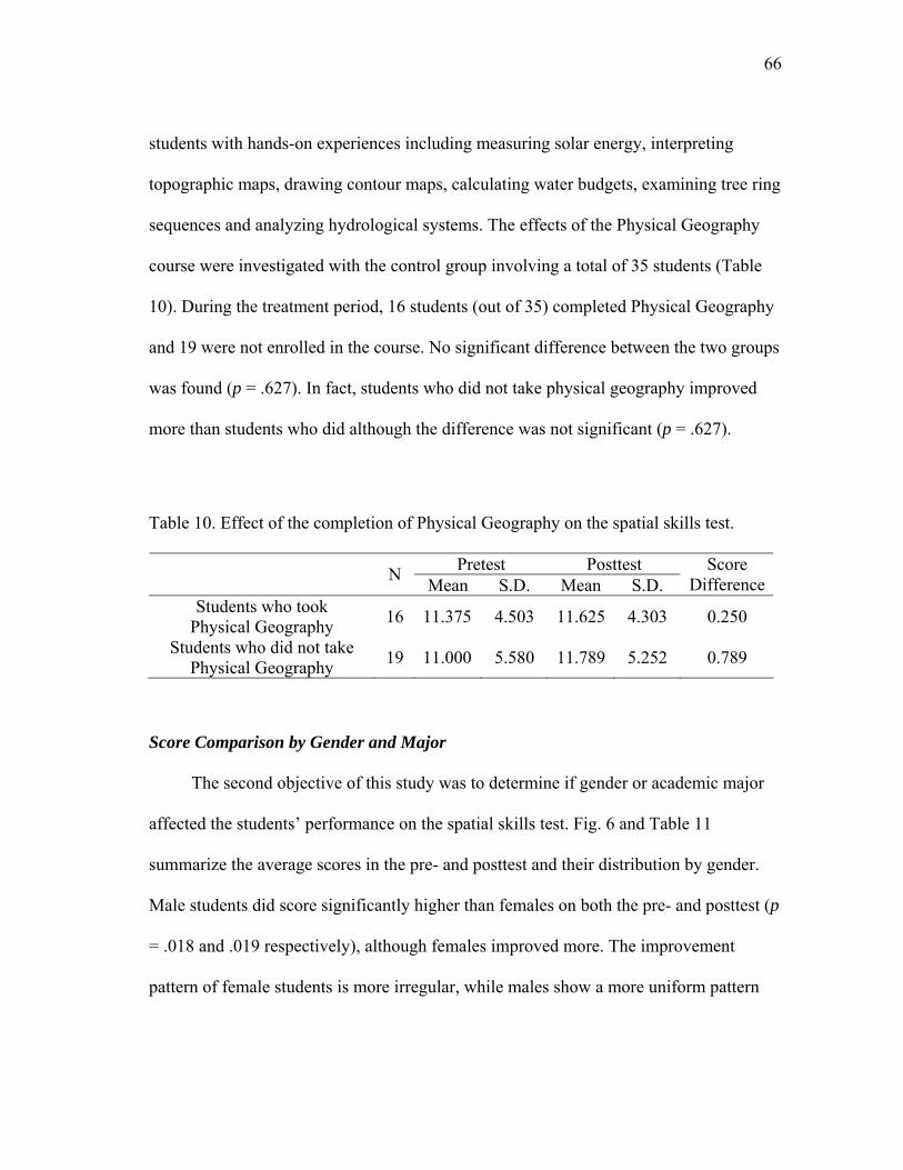
66
students with hands-on experiences including measuring solar energy, interpreting
topographic maps, drawing contour maps, calculating water budgets, examining tree ring
sequences and analyzing hydrological systems. The effects of the Physical Geography
course were investigated with the control group involving a total of 35 students (Table
10). During the treatment period, 16 students (out of 35) completed Physical Geography
and 19 were not enrolled in the course. No significant difference between the two groups
was found (p = .627). In fact, students who did not take physical geography improved
more than students who did although the difference was not significant (p = .627).
Table 10. Effect of the completion of Physical Geography on the spatial skills test.
Pretest Posttest N Mean S.D. Mean S.D. Score
DifferenceStudents who took
Physical Geography 16 11.375 4.503 11.625 4.303 0.250
Students who did not take Physical Geography 19 11.000 5.580 11.789 5.252 0.789
Score Comparison by Gender and Major
The second objective of this study was to determine if gender or academic major
affected the students’ performance on the spatial skills test. Fig. 6 and Table 11
summarize the average scores in the pre- and posttest and their distribution by gender.
Male students did score significantly higher than females on both the pre- and posttest (p
= .018 and .019 respectively), although females improved more. The improvement
pattern of female students is more irregular, while males show a more uniform pattern
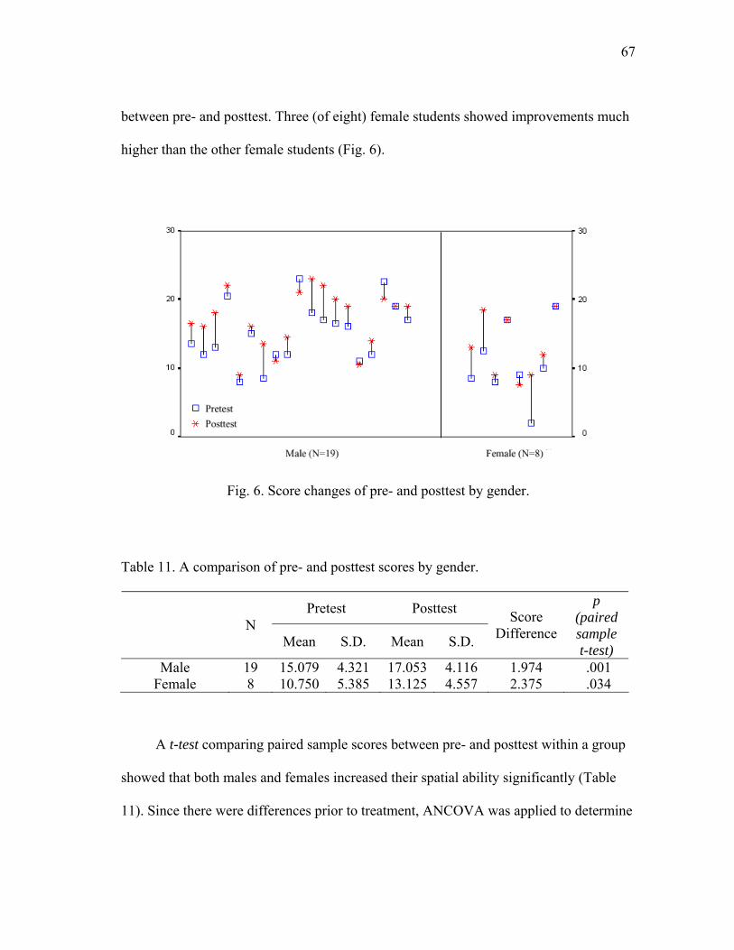
67
between pre- and posttest. Three (of eight) female students showed improvements much
higher than the other female students (Fig. 6).
Fig. 6. Score changes of pre- and posttest by gender.
Table 11. A comparison of pre- and posttest scores by gender.
Pretest Posttest N
Mean S.D. Mean S.D.
Score Difference
p (paired sample t-test)
Male 19 15.079 4.321 17.053 4.116 1.974 .001 Female 8 10.750 5.385 13.125 4.557 2.375 .034
A t-test comparing paired sample scores between pre- and posttest within a group
showed that both males and females increased their spatial ability significantly (Table
11). Since there were differences prior to treatment, ANCOVA was applied to determine

68
whether they were significantly different for improving scores between groups.
ANCOVA revealed that there was no significant difference in score improvement
between the two genders (p = .571) (Table 12). This finding indicates that male and
females students benefit similarly from completing a GIS course.
Table 12. ANCOVA using posttest scores as the dependent variable with the pretest scores as the covariate (by gender).
SS df MSE F p Between groups 1.906 1 1.906 .330 .571 Within groups 138.654 24 5.777
Total 537.167 26
The performance by students having different academic majors was also compared.
The 27 students who completed the GIS course were grouped into three categories:
geography, science and engineering, and humanities. The humanities group was
excluded from further study because it had only 1 student. The average scores of
geography majors and science and engineering majors were compared and are shown in
Table 13. Average score changes from pre- to posttest by major are displayed in Fig. 7.
The relatively higher standard deviations in test scores by students majoring in science
and engineering, a grouping of students majoring in several science and engineering
disciplines, most likely reflected their various fields of study (Table 13).
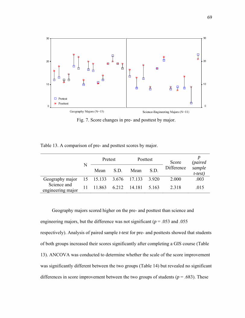
69
Fig. 7. Score changes in pre- and posttest by major.
Table 13. A comparison of pre- and posttest scores by major.
Pretest Posttest N
Mean S.D. Mean S.D.
Score Difference
p (paired sample t-test)
Geography major 15 15.133 3.676 17.133 3.920 2.000 .003 Science and
engineering major 11 11.863 6.212 14.181 5.163 2.318 .015
Geography majors scored higher on the pre- and posttest than science and
engineering majors, but the difference was not significant (p = .053 and .055
respectively). Analysis of paired sample t-test for pre- and posttests showed that students
of both groups increased their scores significantly after completing a GIS course (Table
13). ANCOVA was conducted to determine whether the scale of the score improvement
was significantly different between the two groups (Table 14) but revealed no significant
differences in score improvement between the two groups of students (p = .683). These
70
results indicated that both groups of students benefited comparably from the completion
of the GIS course. It must be noted that, given the small sample size for each gender and
major, the results should be interpreted with caution.
Table 14. ANCOVA using posttest scores as the dependent variable and the pretest scores as the covariate (by major).
SS df MSE F p Between groups 1.033 1 1.033 .171 .683 Within groups 138.795 23 6.035
Total 537.154 25
Correlation between the Spatial Skills Test and GIS Course Achievement
Students’ performance in the spatial skills test was also correlated with each of
their scores in the GIS course: lab exercise score, mid-term grade, and final exam grade.
The results of these correlations are summarized in Table 15. It was expected that (1)
positive correlations between students’ spatial ability and performance in the GIS course
would exist; and furthermore, (2) lab exercise scores, which demanded intensive spatial
cognitive processes, would have a stronger correlation with the spatial ability scores than
exams.
These expectations were only partially supported by empirical findings. Relatively
strong correlations were found between the two spatial skills tests and the final exam
score [.443 (p = .027) and .329 (p = .108)] and between the two spatial skills tests and
lab exercise score [.357 (p = .080) and .405 (p = .044)]. However, correlations with the
mid term scores were weak [.185 (p = .377) and .213 (p = .307)] most likely because this

71
exam occurred before much lab work was done. There was no significant difference in
the correlations between the spatial skills test and either the final exam or the lab
exercise scores.
Table 15. Correlation between spatial skills test and performance of GIS course.
Pretest Posttest Mid-term Final exam Lab exercise
Pretest 1 .852 (p=.000)
.185 (p=.377)
.443 (p=.027)
.357 (p=.080)
Posttest .852 (p=.000) 1 .213
(p=.307) .329
(p=.108) .405
(p=.044)
In addition to these correlations, the impact of the final assignment type on the
spatial skills test was examined, since students of the GIS course were asked to complete
either a project or a paper as their final assignment. During the semester, 17 students
chose a paper assignment and seven students a project assignment. Table 16 shows the
pre- and posttest scores of the two groups. It was expected that students who completed
a GIS project would show higher improvement in spatial ability, since paper assignments
focused more on theoretical aspects of GIS rather than spatial analytical or visual skills.
Table 16. A comparison of pre- and posttest scores by assignment type.
Pretest Posttest N
Mean S.D. Mean S.D.
Score Difference
p (paired sample t-test)
Paper 17 14.205 5.049 15.676 4.260 1.470 .012 Project 7 11.857 5.459 14.214 4.724 2.357 .032
72
A comparison of paired sample t-test scores between pre- and posttest within each
group showed that in both cases students increased their spatial ability significantly
(Table 16). The students who selected to do a project did improve their scores by a
greater amount than students who wrote a paper. Because the sample sizes are small,
however, the difference in the score improvement from pre- to posttest between the two
groups of students taking different assignment types was not significant (p = .778)
(Table 17).
Table 17. ANCOVA using posttest scores as the dependent variable and the pretest scores as the covariate (by assignment type).
SS df MSE F p Between groups .385 1 .385 .081 .778 Within groups 99.606 21 4.743
Total 435.000
Experiment 2: Cognitive-Mapping Test
Video-Analysis of Map-drawing Strategy
Videotaping the participants’ map-drawing process allowed for the analysis of
map-drawing strategies employed by the subjects, including the sequence of map
construction. Post-hoc analysis of the finalized hand-made maps could not have
provided the same amount and types of information. For example, the two maps shown
in Fig. 8, produced by students in this experiment look similar and both might have been
classified as survey maps (according to Applyard 1970), but the analysis of the map-

73
drawing process revealed that the maps were constructed using completely different
strategies. This finding seems counter to that of Foley and Cohen (1984) who assert that
different strategies lead to radically different results.
This study suggests, and demonstrates the efficacy of, a method to accurately
identify the cognitive mapping strategies of individuals. If, as many researchers have
argued, mapping strategies reveal information about the cognitive processes people use
to operate in their environment, it is imperative that researchers categorize the strategies
correctly. Past research has relied on evaluation of the (finished) maps produced by
individuals to identify mapping strategies. Unfortunately, as this study demonstrates, it is
often extremely difficult to determine a subject’s strategy from the map she or he draws.
Videotaping subjects while they map does add time and effort to the experimental design,
but modern digital video equipment is affordable enough that researchers can employ
more than one camera during mapping sessions, reducing the time necessary to collect
data. In addition, digital images can be viewed repeatedly, allowing researchers to
extract detailed information that might otherwise go unobserved. Finally, digital motion
pictures are easily edited so that compelling presentations demonstrating the results of
the research can be developed and shown to other researchers.
The inability to determine a subject’s mapping strategy from a finished map also
means that it is often impossible to detect changes in a subject’s mapping strategy over
time. The pilot test demonstrated that some subjects changed their map-drawing strategy
after the completion of a computer cartography course. Only through the analysis of
tapes of subject’s map-drawing process, was it possible to detect these changes.

74
Fig.
8. M
aps c
reat
ed b
ased
in a
regi
onal
(A) a
nd a
hie
rarc
hica
l (B
) app
roac
h.
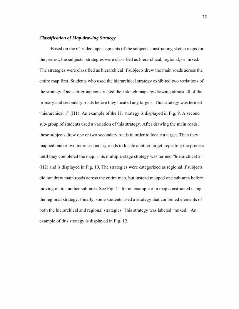
75
Classification of Map-drawing Strategy
Based on the 64 video tape segments of the subjects constructing sketch maps for
the pretest, the subjects’ strategies were classified as hierarchical, regional, or mixed.
The strategies were classified as hierarchical if subjects drew the main roads across the
entire map first. Students who used the hierarchical strategy exhibited two variations of
the strategy. One sub-group constructed their sketch maps by drawing almost all of the
primary and secondary roads before they located any targets. This strategy was termed
“hierarchical 1” (H1). An example of the H1 strategy is displayed in Fig. 9. A second
sub-group of students used a variation of this strategy. After drawing the main roads,
these subjects drew one or two secondary roads in order to locate a target. Then they
mapped one or two more secondary roads to locate another target, repeating the process
until they completed the map. This multiple-stage strategy was termed “hierarchical 2”
(H2) and is displayed in Fig. 10. The strategies were categorized as regional if subjects
did not draw main roads across the entire map, but instead mapped one sub-area before
moving on to another sub-area. See Fig. 11 for an example of a map constructed using
the regional strategy. Finally, some students used a strategy that combined elements of
both the hierarchical and regional strategies. This strategy was labeled “mixed.” An
example of this strategy is displayed in Fig. 12.

76
Fig.
9. H
iera
rchi
cal a
ppro
ach
1 (m
ajor
and
seco
ndar
y ro
ads d
raw
n be
fore
feat
ures
).
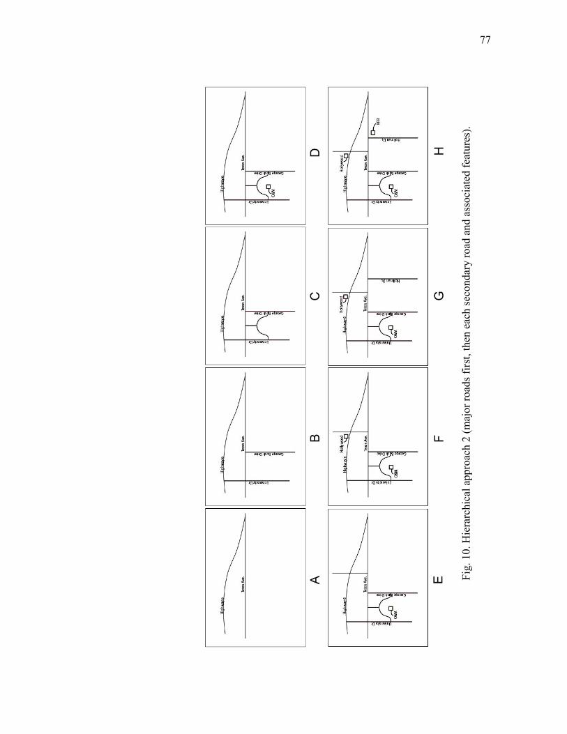
77
Fig.
10.
Hie
rarc
hica
l app
roac
h 2
(maj
or ro
ads f
irst,
then
eac
h se
cond
ary
road
and
ass
ocia
ted
feat
ures
).
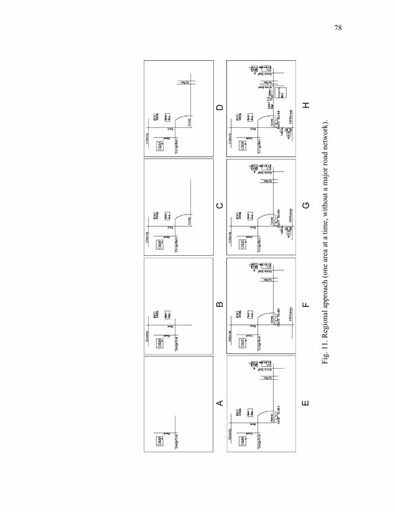
78
Fig.
11.
Reg
iona
l app
roac
h (o
ne a
rea
at a
tim
e, w
ithou
t a m
ajor
road
net
wor
k).

79
Fig.
12.
Mix
ed a
ppro
ach.

80
The majority of the subjects (47 of 64) used one of the hierarchical strategies. The
H2 strategy was the most frequently observed. It is very similar to the strategy described
by Taylor and Tversky (1992) who reported that when subjects were asked to describe
their cognitive maps verbally, they began their maps with larger border features,
continued with the major roads, and then placed the smallest features, the buildings. It
seems obvious that one or two main roads constructed at an early stage could serve as a
reference point for the location of other places. Thus, the relationship between main
roads and details (secondary roads) can be understood as a function of hierarchy.
Excerpts of three typical transcripts from students using the H2 strategy illustrated the
multiple-stage process that characterizes this mapping strategy:
I drew Highway 6 first and then I drew the bypass and Texas Avenue. Those are the main roads that go through the town. I related everything else off those two roads. I started drawing the next level roads down, which is the next main highway in the area that was discussed, which is Highway 30, also known as Harvey (road). I drew the movie theater next it was… And I drew George Bush (Drive), which is the next main road needed to relate where the O&M building was. And I drew Bizzell connecting it.
I drew Highway 6 first because this is one of main highways where most
people come in off of. Then I drew Texas (Ave.), another pretty much main road through College Station. University (Drive) runs along the campus as well as George Bush (Drive). Harvey road, which can take you to Sam’s and Hollywood movie…. Then Holleman (Drive), that’s connected to HEB. I drew New Main (road), which runs close to the O&M building. And I drew the feeder of Highway 6 running through Hollywood Movie.
I drew Texas Ave. first because I feel like that it’s the most major road in
town. And the BestBuy and HEB are off that road. And then …by drawing Texas Ave. I could add … the other major roads in town …off that way I can find out where the school is. Because I know on all four sides of the school there are major roads. When I have the major roads in town, I could draw the small roads of the university … then I could label the O&M building. … I drew Highway 6 because that’s where the movie theater is off. So basically I drew the major roads in town first. … I think (Farm to Market Road) 2818’s right there. Now it’s like a skeleton
81
of the city. … That was Holleman (Drive). I knew that HEB is next Holleman. So, BestBuy… right off Texas (Ave).
In contrast to those who used the H2 strategy, subjects who used the H1 strategy
mapped almost all of the roads before they placed any target monuments. This strategy
represents the most stereotypically hierarchical strategy used by any of the subjects. The
students who used the H1 strategy seemed to have more flexible and precise knowledge
of the area than other subjects. The following is an excerpt of a typical transcript from a
student using the H1 strategy:
Anytime I think about the city I kind of think outskirts first and kind of work in. … If you start inside, you might be too detailed. … I tried to have some scale, obviously not much. I think that starting inside, all of a sudden you’ve got all this junk packed in, and then you know you have stuff way off the page. … If I put the roads in the first, I can better reference where the stuff is. If I put the stuff in and it gets off at the first, the whole image after while is gonna get…
By drawing one or two major roads first, using the H1 and H2 strategies, students
could reduce the load on their working memory. The H1 and H2 strategies also provide
physical limitations on the range of potential drawing and consequently reduce the size
of the search space to be considered. However, since the H1 strategy requires a longer
planning horizon and a more systematic sequence of drawing, this strategy can be
regarded as more plan-based than the H2 strategy.
Most students who used the regional strategy (5 of 7) began by drawing the O&M
building which is where the subjects were physically located when they were drawing
their maps. The subjects gave a variety of reasons for beginning their sketch maps with
the O&M Building or the campus:
I started with the O&M building because I’m familiar with this area.
82
Probably because that’s where I am at. I liked to know where the campus is because it seems like everything is
related to where the campus is... Kyle Field is a pretty good landmark here. Coming into College Station if you don’t know where you going. If you see that then you know where you’re at. I drew that first I guess.
I drew A&M (campus) first because that’s the center piece to me. It is kind
of base, everything around where it is in relation to A&M … That (campus) is really the first thing came into my head. (I) drew (campus) first and drew roads around it. There wasn’t really a specific reason. It seems the easiest for me to do it that way.
From the content of these interviews, it appears that participants using the regional
strategy begin by drawing important or familiar targets first. One of these participants
gave a different reason for beginning at one corner:
I started with the O&M building because it was just the first one in the list (of targets students were asked to locate). So I went systematically through it (list of targets). Kind of went in that order.
Whereas participants with other strategies completed a major road by one stroke,
those using the regional strategy constructed major roads segment by segment. The
following two excerpts give an idea of why they did not draw a road with a single stroke,
and were taken from answers to the questions: why didn’t you complete Texas Ave. all
at once? Why did you draw only half of University Drive?
Because I was trying not to forget anything on the way. So I was thinking. You know, up to a point like did I forget anything or how far am I going to have to go to include everything.
Because I didn’t know how far down I was going to have Texas Ave.,
because nothing is to scale. That’s why I didn’t draw all University (Drive).
In addition, participants with the regional strategy encoded the area as a set of sub-
regions occupying geometrical divisions of the map such as the top half, bottom left

83
quadrant, etc. There are two plausible explanations for this type of drawing pattern. One
is that starting at the upper-left corner may be related to habits of reading order, that is,
top-down, left-right (Kugelmass and Lieblich 1979). The other is that problem solving
based on the spatial proximity of elements in the task is more often observed in novices
than in experts who focus more on the functional nature of the elements in the task
(Egan and Schwartz 1979). Just as local maximization can lead to global non-optimality,
localized map-drawing might not be globally optimal (Anderson 1991).
Some of the participants using the regional strategy drew and explained their maps
as if they were driving around the area:
Then the shopping center and on the other side of Texas (Ave.) ... kind of like, if I was driving down Texas (Ave.), kind of what I see to the left of me.
I think that it’s because I am from Fort Worth and that’s the direction I come
in. So that’s just what I think of what I know I’m going to pass, I guess that’s how I normally see it.
This strategy may be related to the “mental tour” suggested by Linde and Labov (1975)
and Levelt (1982). According to them, when people describe an apartment, for example,
some of them start at the front door and then imagine moving through the apartment
room by room.
Even though users of the regional strategy frequently started drawing in a corner of
the paper without constructing a framework for the entire area, most of them seem to
envision the whole map from the beginning:
Definitely I thought about it (layout) in my head before I drew it. It’s like all already there in my brain, I just have to start somewhere. … I
knew that I had to fit in Hollywood 16 (movie theater) eventually. So I need space in bottom left and corner. That’s why I picked that top right corner relative to

84
bottom left corner leaving space available for the Hollywood 16. I tried to keep in mind where the full extent of the map would have to be
because all the way on the right, you’ll see that, it has Hollywood 16 (movie theater). I knew that would have to be on the right. And I knew Best Buy, HEB, so I just kind of kept those in mind where those were. Make sure that all those were included on the side.
The mixed strategy was similar to the hierarchical strategy in that subjects began
by drawing the main roads. The mixed strategy, however, also displays similarities with
the regional strategy in that subjects completed a sub-area or half of the map before they
moved to another area.
Quantitative Comparison among Strategies
Variability among strategies could result from the different spatial cognitive ability
of mappers. For example, the regional strategy is thought to be a bottom-up approach
more frequently used by novices (Chase and Chi 1981; Chi et al. 1981). However, the
qualitative data provided by the interviews did not support this argument. Subjects of
both strategies have a similar grasp of the spatial details of the study area. One
difference between the hierarchical mappers and the regional mappers is that the subjects
using the hierarchical strategy seem to draw their maps more efficiently. This difference
is illustrated by the mean time these two groups took to draw their maps. The average
time to construct maps for all students was 361s. The mean time for users of the
hierarchical strategies was 343s; for the users of the regional strategy was 478s. The
difference was significant (p = .043).
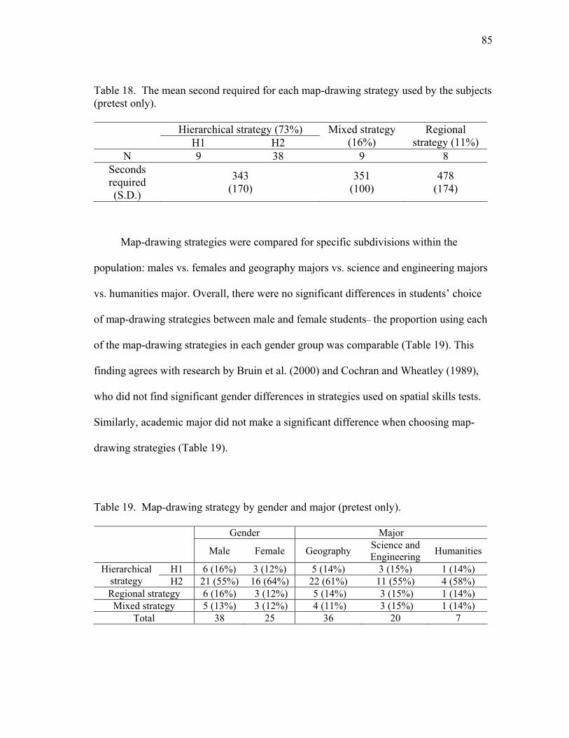
85
Table 18. The mean second required for each map-drawing strategy used by the subjects (pretest only).
Hierarchical strategy (73%) H1 H2 Mixed strategy
(16%) Regional
strategy (11%) N 9 38 9 8
Seconds required (S.D.)
343 (170)
351 (100)
478 (174)
Map-drawing strategies were compared for specific subdivisions within the
population: males vs. females and geography majors vs. science and engineering majors
vs. humanities major. Overall, there were no significant differences in students’ choice
of map-drawing strategies between male and female students– the proportion using each
of the map-drawing strategies in each gender group was comparable (Table 19). This
finding agrees with research by Bruin et al. (2000) and Cochran and Wheatley (1989),
who did not find significant gender differences in strategies used on spatial skills tests.
Similarly, academic major did not make a significant difference when choosing map-
drawing strategies (Table 19).
Table 19. Map-drawing strategy by gender and major (pretest only).
Gender Major Male Female Geography Science and
Engineering Humanities
H1 6 (16%) 3 (12%) 5 (14%) 3 (15%) 1 (14%) Hierarchical strategy H2 21 (55%) 16 (64%) 22 (61%) 11 (55%) 4 (58%) Regional strategy 6 (16%) 3 (12%) 5 (14%) 3 (15%) 1 (14%)
Mixed strategy 5 (13%) 3 (12%) 4 (11%) 3 (15%) 1 (14%) Total 38 25 36 20 7

86
Changes of Map-drawing Strategies
After finishing either the GIS or cartography course, the participants produced
their second maps. A total of 46 students completed both the pre- and posttest of the
cognitive-mapping experiment. Table 20 and 21 show which strategies were used by
participants during the pre- and posttest, and how their strategies changed after
completion of either the GIS or cartography courses.
Forty one percent of the students (19 of 46) changed their map-drawing strategies
for the posttest. It was assumed that learning GIS would cause students to change their
map-drawing strategies from regional to hierarchical, from mixed to hierarchical or from
hierarchical 2 to hierarchical 1. Ten of 13 changes observed within the GIS group
supported this research assumption. However, the same pattern was not found in the
group that completed only the cartography course; only three of six changes in the
cartography group agreed with this research assumption (Table 21).
Table 20. Map-drawing strategies in the pre- and posttest.
Hierarchical strategy H1 H2
Mixed strategy
Regional strategy
Pretest 3 10 1 3 Cartography Posttest 1 11 1 4
Pretest 3 15 4 3 GIS Posttest 6 14 3 2 Pretest 2 2 Cartography
and GIS Posttest 4

87
Table 21. Direction of map-drawing strategy changes.
Direction of map-drawing strategy changes N
Hierarchical 1 to Regional 2 Hierarchical 2 to Regional 1
Hierarchical 2 to Hierarchical 1 1 Cartography
(6 of 17) Regional to Hierarchical 1 2
Hierarchical 1 to Hierarchical 2 1 Hierarchical 2 to Hierarchical 1 3
Hierarchical 2 to Mixed 1 Hierarchical 2 to Regional 1 Mixed to Hierarchical 2 3
Regional to Hierarchical 1 1
GIS (11 of 25)
Regional to Mixed 1 Cartography and GIS
(2 of 4) Hierarchical 2 to Hierarchical 1 2
About half (11 of 19) of the participants who changed their map-drawing strategies
were interviewed to investigate the underlying reasons for their strategy changes. The 11
students were randomly selected from either the GIS or the cartography group. The
analysis of the interview data is presented jointly because there was no significant
difference between the GIS and cartography group in terms of reasons for their strategy
changes.
Interestingly enough, five of the 11 interviewed participants could not explain the
reason they used different map-drawing strategies for their second maps:
I have no idea. (A participant who changed from regional to H2) It’s just… at the first time the campus popped up in my head first. But at the
second time University Drive came up first. It’s hard to explain that. (A participant who changed from regional to H2)
I don’t know. Maybe I was tired. (A participant who changed from H2 to
88
regional) It makes more sense to me to draw all at once. I am not sure why I drew two
increments [segments] the first time. (A participant who changed from regional to mixed)
Even though the interval between pre- and posttest was relatively long (about three
months), testing effects were found in some cases. Three (of the 11 interviewed
participants) attributed changes in their map-drawing strategies to learning effects from
their pretest:
I just realized that I thought about the last time I did this. And I realized that I wasted a bunch of space I could use to put more details on. (A participant who changed from H1 to H2)
I just think that I learned what I did wrong about the first one. (A participant
who changed from H2 to mixed) I needed a lot more space. I realized that I’ve already drawn Texas Ave. first
before I even thought about how much space I would need until… it was too late. … Because this time [posttest] I just wanted to make sure that I had enough space to get everything on that. I wanted to get my grid first. (A participant who changed from mixed to H2)
Only one student in the same group attributed the change in the map-drawing
strategy to GIS experience:
[GIS experience] …getting me to think like where things are compared to another places. At the beginning I had to do it like when I was moving in my car approaching something that’s what I saw. The GIS course helped me see the big picture. (A participant who changed from regional to H1)
Even though the reasons that some participants used for adopting different
strategies for their second maps were not clear, impacts of their GIS experience on map-
drawing were easy to find during interviews. For example, some participants either
added a north arrow or used different types of north arrows as orientation for their

89
second maps:
I think that I used to do this in class, GIS. From everything I read covered in all the classes… it should always have a
north arrow. I guess that it’s working with ArcView. It looked like that. I think from classes like… I learned more than one compass through GIS
[class]. I guess getting used to making more maps; you need to know where you
oriented it… just kind of reference.
The influence of GIS courses was also found on space usage:
Definitely in that [GIS] class one thing that it wants you [to do] is to use as much as area you can to show what you have. And I think that is probably why I drew a bigger space on this one here.
Remote sensing coursework also affected some students’ viewpoints:
I saw them [air photos] in remote sensing class. Because I see it from overhead, that’s more how you draw a map.
Looking from space, you know, satellites [images from remote sensing
class] help you see holistically instead of what’s right around O&M.
Relationship between Map-drawing Strategy and Spatial Ability
The relationship between students’ map-drawing strategies and their performance
on the spatial skills test was investigated, and the findings are summarized in Table 22.
A total of 39 students finished both the spatial skills test and the cognitive-mapping test.
They were grouped by type of strategy, and the average score of each map-drawing
group was calculated. Contrary to expectations, students who used the regional strategy
scored higher in the spatial skills test than those using either hierarchical or mixed

90
strategies. However, the score difference between the four different strategies was not
significant (p = .284). It should be emphasized that this insignificant difference may
have been caused by the small sample size used in the study.
Table 22. A comparison of posttest scores by map-drawing strategies.
Strategy N Mean S.D. Hierarchical 1 6 16.666 2.750 Hierarchical 2 23 14.260 5.065
Mixed 6 16.250 4.535 Regional 4 19.875 1.887
Table 23. ANOVA for posttest scores by map-drawing strategies.
SS df MSE F p Between groups 80.062 3 26.687 1.316 .284 Within groups 750.389 37 20.281
Total 830.451 40
91
CHAPTER V
DISCUSSION AND CONCLUSIONS
This chapter provides interpretation of the results of the two previous research
experiments and their discussion in the context of the research questions. The discussion
also connects the findings of this study with the literature reviewed in Chapter II. This is
followed by a summary and conclusions. The results of this study are discussed in the
same order established when presenting the research questions. The research questions
that were previously framed for this study are as follows:
1. Will GIS learning affect students’ spatial ability?
a. Will completion of a GIS course affect the spatial ability of college
students? Will completion of a cartography course be equally effective as
a GIS course?
b. Will these effects be different for male and for female students? Will
these effects differ by students’ academic majors?
c. Is there a relationship between students’ spatial abilities and learning
achievement in a GIS course?
2. Will GIS learning affect students’ spatial problem solving?
a. Will completion of a GIS course affect the map-drawing strategy of
college students?
b. Is there a relation between students’ map-drawing strategies and spatial
ability?
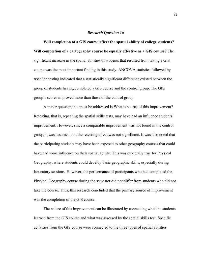
92
Research Question 1a
Will completion of a GIS course affect the spatial ability of college students?
Will completion of a cartography course be equally effective as a GIS course? The
significant increase in the spatial abilities of students that resulted from taking a GIS
course was the most important finding in this study. ANCOVA statistics followed by
post hoc testing indicated that a statistically significant difference existed between the
group of students having completed a GIS course and the control group. The GIS
group’s scores improved more than those of the control group.
A major question that must be addressed is What is source of this improvement?
Retesting, that is, repeating the spatial skills tests, may have had an influence students’
improvement. However, since a comparable improvement was not found in the control
group, it was assumed that the retesting effect was not significant. It was also noted that
the participating students may have been exposed to other geography courses that could
have had some influence on their spatial ability. This was especially true for Physical
Geography, where students could develop basic geographic skills, especially during
laboratory sessions. However, the performance of participants who had completed the
Physical Geography course during the semester did not differ from students who did not
take the course. Thus, this research concluded that the primary source of improvement
was the completion of the GIS course.
The nature of this improvement can be illustrated by connecting what the students
learned from the GIS course and what was assessed by the spatial skills test. Specific
activities from the GIS course were connected to the three types of spatial abilities
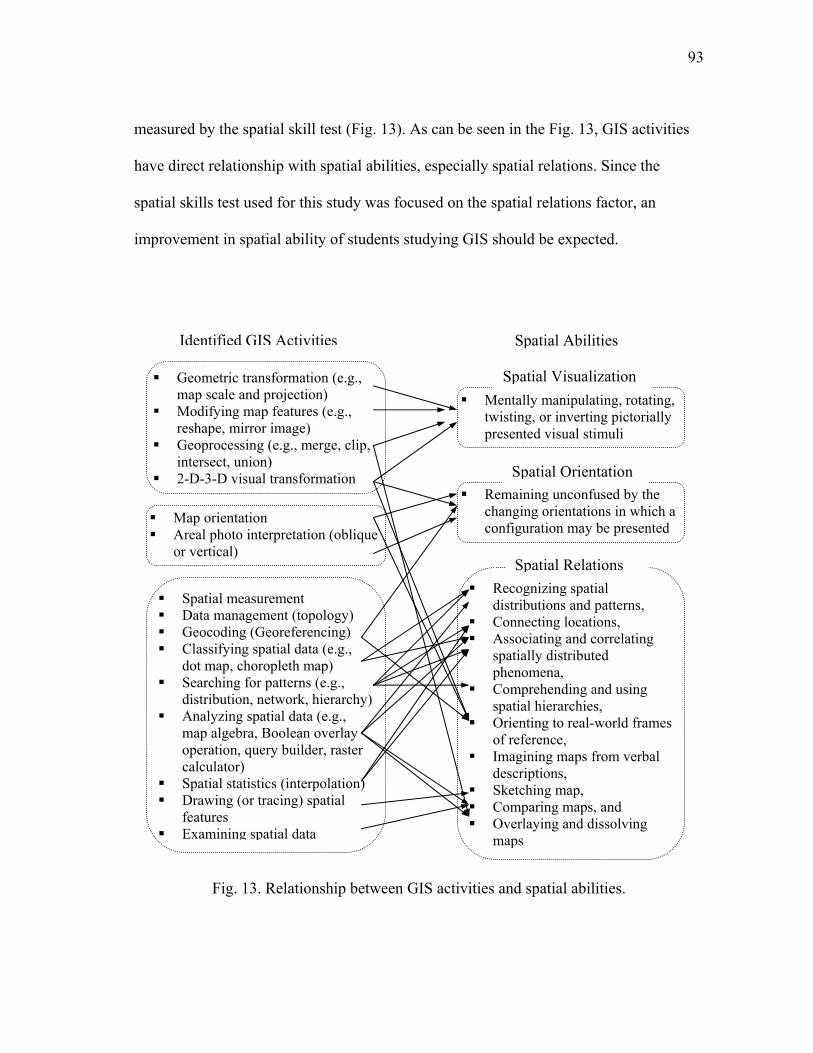
93
measured by the spatial skill test (Fig. 13). As can be seen in the Fig. 13, GIS activities
have direct relationship with spatial abilities, especially spatial relations. Since the
spatial skills test used for this study was focused on the spatial relations factor, an
improvement in spatial ability of students studying GIS should be expected.
Identified GIS Activities Spatial Abilities
Fig. 13. Relationship between GIS activities and spatial abilities.
Map orientation Areal photo interpretation (oblique
or vertical)
Geometric transformation (e.g., map scale and projection)
Spatial Visualization Mentally manipulating, rotating,
twisting, or inverting pictorially presented visual stimuli
Modifying map features (e.g., reshape, mirror image)
Geoprocessing (e.g., merge, clip, intersect, union)
2-D-3-D visual transformation
Spatial measurement Data management (topology) Geocoding (Georeferencing) Classifying spatial data (e.g.,
dot map, choropleth map) Searching for patterns (e.g.,
distribution, network, hierarchy) Analyzing spatial data (e.g.,
map algebra, Boolean overlay operation, query builder, raster calculator)
Spatial statistics (interpolation) Drawing (or tracing) spatial
features Examining spatial data
Remaining unconfused by the changing orientations in which a configuration may be presented
Spatial Orientation
Recognizing spatial distributions and patterns,
Connecting locations, Associating and correlating
spatially distributed phenomena,
Comprehending and using spatial hierarchies,
Orienting to real-world frames of reference,
Imagining maps from verbal descriptions,
Sketching map, Comparing maps, and Overlaying and dissolving
maps
Spatial Relations

94
However, the strength and type of interaction between GIS learning and
improvement of spatial abilities varied widely. Certain aspects of the interaction were
more easily verified than others. For example, it turned out that GIS learning was
particularly helpful for specific spatial tasks such as finding the best location for an
activity when given diverse spatial information (item #2), identifying spatial correlations
between sets of maps (item #5), and identifying spatial data types such as point, line and
polygon (item #7) (See Table 9). The findings of this study almost coincided with the
prediction of the GIS instructor, who expected improvements by GIS students on items
item #1 (map overlay operation), item #2, and #7. Assuming that students already had
enough cartographic/map-reading skills, the instructor did not emphasize these skills in
class, and thus did not predict improvements on items such as orienting to real world
frame of reference (item #3) and imagining maps from verbal description (item #4). It is
interesting to note that items #1 (map overlay operation) and #2 (finding the best
location) were believed to measure the same trait as “overlaying and dissolving maps”
but led to different results. GIS students outperformed their control group counterparts
on item #2, but not on item #1. This outcome may have been caused by similarity
between item #2 and examples of spatial analysis which GIS students worked out during
their lab exercises. Since students dealt with similar examples during their labs, they
might have felt more comfortable when confronting item #2 than item #1. This
hypothesis was supported by anecdotal discussions with some of the test takers. This
finding supported previous research by Albert and Golledge (1999) who found no
significant differences in performance between GIS-users and non-users for similar

95
types of map overlay operations.
The better performance by GIS students on item #5 (identifying spatial
correlations) indicated that GIS learning positively affected students’ abilities to
“recognize spatial distributions and spatial patterns,” and to “compare, associate, and
correlate spatially distributed phenomena.” This finding conflicts with research by Baker
(2002), who did not find improvements of this type.
Cartography students also performed better than the control group on item #5
(identifying spatial correlations). In Computer Cartography, students were exposed to a
variety of spatial data and maps during both lectures and labs. Consequently, they may
have increased their spatial ability to find spatial patterns and relations. However,
significant differences between the cartography group and the control group were not
found for items #3 (orientating to real world frame of reference) and #4 (imagining maps
from verbal description); these items were also believed to require students to use their
cartographic/map-reading skills. Actually for item #3, cartography students raised their
scores (the rate of correct answers was 19.5 percent and 33.3 percent for pre- and
posttest respectively), but this increase was not statistically significant when compared
to the control group (who scored 31.1 percent and 37.1 percent respectively). In regard
to item #4, and taking into consideration the rates of 86 percent and 72 percent correct
answers by cartography students in the pre- and posttest, it can be assumed that
cartography students already had enough of the cartographic/map-reading skills required
for this item.
The better performance by the GIS group on item #7 (identifying spatial data type)
96
indicated that GIS learning could advance students’ spatial cognitive abilities to
“imagine maps from a verbal description,” and to “recognize spatial patterns.” The GIS
students who clarified concepts for spatial data may have become proficient in
identifying structures of spatial information.
This study verified that GIS learning positively affected the spatial ability of
students. This finding supports previous research asserting strong correlations between
GIS-based learning and spatial thinking (Hall-Wallace and McAuliffe 2002), and
between learning with GIS and spatial-visual thinking skills (Hagevik 2003).
Research Question 1b
Will these effects be different for male and for female students? Will these
effects differ by students’ academic majors? The second research question asked if
students of different gender or fields of study benefited differently from completion of a
GIS course. Very few differences in spatial skills improvement were found when
comparing students of different gender or different major.
With regard to gender, male students performed better than females on pre- and
posttests (p = .018 and p = .019 respectively). However, ANCOVA did not find
significant gender-related differences in students’ score improvements (p = .571). It
should be noted that, although differences in the pre- and posttest were statistically
significant, there was a mixed pattern in the performance of the two groups with some
female students performing well and some male students performing poorly on the
spatial skills test. These results are in agreement with findings by Hagevik (2003) and

97
Allen (1974) who reported higher scores for males on the spatial reasoning tests. Other
studies (e.g., Vincent 2004), however, found little or no difference in the spatial ability
of males and females.
In general, males outperform females in spatial visualization ability (Chadwick
1978; Harris 1978; Kali and Orion 1996; Liben 1981; Maccoby and Jacklin 1974;
McGee 1979a; Sherman 1980). Connor et al. (1977) and Goldstein and Chance (1965)
argued that males tend to get marks closer to the maximum score than females on pretest,
and since females are farther from the maximum score, they potentially have larger room
for improvement after training. For example, Saccuzzo et al. (1996) reported that men
outperformed women in the pretest, but that women showed a much higher rate of
improvement after training.
This study found that male students, even though having scored higher than
females on the pretest, still improved their spatial ability as much as female students
(Table 11). Both males and females increased their spatial ability significantly after the
GIS learning experience (p = .001 and p = .034 respectively). Therefore this study can
argue that both males and females have substantial room for improvement in spatial
ability through training.
Irregular patterns of improvement were identified within female students: some of
them improved substantially while others remained at the same level or even scored
lower. These differences among females may be related to their computer skills or
attitudes toward computer usage. However, tests evaluating the participants’ computer
skills or attitudes were not conducted during the experiment, and in the context of this

98
research this issue remains unresolved.
Participants’ performance on the spatial skills test was also analyzed according to
their different academic majors. A paired sample t-test followed by ANCOVA showed
that both the geography majors and the science and engineering majors improved their
spatial ability after the completion of a GIS course, and that there were no significant
differences in the rate of improvement of the two groups. This finding agrees with
previous research, in which no relationship between fields of study and spatial cognitive
test scores in the context of GIS were found (e.g., Hagevik 2003; Vincent 2004).
When analyzing the distribution of scores of geography and science and
engineering students, it was found that the former showed smaller standard deviations
than the latter. This difference may be attributed to the more varied background that
science and engineering students were previously exposed to, given that this group of
students was composed of individuals majoring in a variety of disciplines. If spatial
abilities are important in the use of GIS (Montello et al. 1999), this finding suggests that
GIS educators should be aware of the wider variation in spatial ability of non-geography
students.
Research Question 1c
Is there a relationship between students’ spatial abilities and learning
achievement in a GIS course? The third research question dealt with the relationship
between the participants’ spatial ability and their scores in the GIS course. Students’
performance on the spatial skills test was correlated with their lab exercises scores, mid-

99
term score, and final exam score. The impact of the type of final assignment (paper vs.
project) on the spatial skills test was also examined. It was hypothesized that (1) positive
correlations between students’ spatial abilities and their performance in a GIS course
would exist; (2) the posttest of spatial ability would have a stronger correlation with lab
exercises than class exams because lab exercises demand more intensive hands-on
spatial cognitive processes; and (3) the participants who chose a project instead of a
paper as their final assignment would have a greater increase in their spatial ability than
their counterparts.
The results of this study can be compared to some previous research. For example,
Hall-Wallace and McAuliffe (2002) found positive correlations between students’ spatial
ability and performance in a posttest that covered material similar to what was learned
during a set of GIS-related activities. Orion et al. (1997) also found significant
correlations between overall geology class scores and spatial skills tests. Conversely,
research by Vincent (2004) found very little relationship between students’ spatial ability
scores and their lab and exam scores in a GIS course.
The first hypothesis that this study advanced is only partially supported by
empirical evidence. Relatively strong correlations exist between the two spatial skills
tests and the final exam [.443 (p = .027) and .329 (p = .108)] and between the two spatial
skills tests and the lab exercises [.357 (p = .080) and .405 (p = .044)]. However,
correlation with the mid term is weak [.185 (p = .377) and .213 (p = .307)]. It is
noticeable that correlations between the spatial skills test and the lab exercises became
stronger after GIS learning experience. These findings indicate that the participants

100
improved their spatial ability during the experimental semester.
The second hypothesis is supported by the results of correlation analyses. Posttest
spatial ability has a stronger correlation with lab exercises than class exams. Considering
that the lab exercises were relatively simple (i.e., demanding few spatial cognitive
processes) it is possible that the correlation could have been higher than 0.044. The
simplicity of some of the problems faced by students in the labs was mentioned by
several study participants.
The labs from the textbook we used were very basic. They were a good introduction. They were very easy and very basic. … Well, the labs talk you through, and, it’s not just what theoretically you’re trying to do, but it’ll tell you everything from what to click on, to what file you’re looking for.
You get instructions for lab. You just go bang, bang, bang, and do them.
And turn it in, you know, do the minimal amount possible and then, you know, when comes time to do it, and put it all together, you’ve forgotten… Or maybe never really learned it and just followed the steps.
It [doing labs] was just more, just getting familiar with software instead of
actually having to use it. However, the difference was not stronger than assumed.
It is also interesting to note the strong correlation between the final exam and the pretest
of spatial ability which was administered before the actual treatment. Since the final
exam required fewer of the spatial abilities acquired during the GIS experiences than lab
exercises, exam scores should be more directly correlated to the students’ intellectual
potential already reflected in the pretest.
Regarding the final assignment, because paper assignments focus more on GIS
theoretical content than on the analytical or visual aspects of GIS, those students who
completed a GIS project were expected to show greater increases in spatial ability than
students who completed a paper. ANCOVA, however, revealed that there is no
101
significant difference in score improvement between the paper and project groups (p
= .778).
Even though an analysis based on quantitative data did not show significant
differences, qualitative data obtained from student interviews provided some additional
useful information. This is particularly significant for the types of projects assigned to
students, the types of experiences students gained from a project, the relationships
between labs and projects, and how project assignments could be enhanced.
Lab is just you know do this, click this. It…this [project] is more like real world situations. You know, I was pretending I was with a business, and I had to figure out where to put a new pizza store location. That’s what I did for mine [project].
Working on the project made me do that [combining multiple labs], so, and
that’s what helped. I’ve learned more during the project than I learned what to do during class.
Because this is actually…you know, like … analyzing. I thought it would be a good opportunity to fully assess what I had gained in
390 [Introduction to GIS class] in order for me to assess if I should go on to 475 [advanced GIS class]. And uh, I think I did just that. I felt that doing a report would just, would be more of a…something I could just research. As far as the project goes, I would have to use stuff that I learned in lab as well as stuff I learned in research, and bring them all together.
Educational Implications: GIS Lab Exercise, Project, and Their Relationship
Usually an individual lab exercise is developed to cover a single topical procedure
such as changing map projection, georeferencing, network analysis, etc. Completing a
lab exercise implies that students will (1) recognize the same or similar problems (or
procedures) when they encounter real-world situations later, and (2) apply the specific

102
procedure or application they learned from the lab appropriately to the problem. In
reality, however, the lab exercises are often overly simplified whereas real world
projects are so complicated that students cannot recognize the problem and apply the
proper procedure or application (Forer and Unwin 1999).
The development of lab exercises typically follows a kind of “divide-and-conquer”
approach that divides real-world problems into smaller sub-problems, each of which is
covered by a single lab exercise. In addition, lab exercise development depends on the
principles of “transfer” assuming that knowledge or skills from lab exercises can be
transferred to real-world projects. The divide-and-conquer approach is often applied in
artificial intelligence to solve large problems efficiently. The solution of the entire
problem is obtained by solving smaller sub-problems. The procedures that solve mini-
problems are combined to get larger applications, and then these are combined again to
get even larger procedures (Kammár et al. 1998). However, the divide-and-conquer
approach cannot guarantee the transition from solving a collection of simple sub-
problems to a solution to a complicated larger problem. Bednarz (1997, 2001) points out
the same problem:
Students knew how to do it (one can assume that from the fact that they completed the course with an above average grade), but they could not state what it was they could do. … The step-by-step instructions offered in the lab served as “training wheels” but it was not until the wheels were removed and students had to pedal off by themselves that real learning took place.
The use of learned outcomes to facilitate learning in other situations is generally
referred to as transfer of learning. When students (1) are taught in multiple contexts or
from multiple examples, (2) are guided to use multiple skills (labs) rather than a single

103
lab procedure for their projects, and (3) work with actual local data, they will be more
able to transfer knowledge and skills successfully from labs to projects and from projects
to real-world situations (Anderson et al. 1996; Bransford et al. 2000; Brown and Kane
1988; Gick and Holyoak 1983; Lodico et al. 1983; McCombs 1996; Nixon and Kanak
1981; Reed and Bolstad 1991; Sweller and Cooper 1985).
Research has indicated that transfers across contexts are especially difficult when a
subject is taught in only a single context rather than in multiple contexts (Anderson et al.
1996; Nixon and Kanak 1981). Transfer of learning is enhanced when learning involves
multiple examples rather than a single example (Reed and Bolstad 1991; Sprio et al.
1992; Sweller and Cooper 1985). These findings provide useful guidelines to the
development of GIS lab exercises that would allow GIS learners to develop usable and
conditionalized knowledge supporting transfer of learning. For instance, students can be
asked to elaborate on the multiple aspects of one problem, then be provided with similar
problems and asked for slightly different solutions, and then finally be required to
deduce to what degree their learning may be applicable to the real-world.
There are few real-world problems that one can solve with a single GIS procedure.
If students are guided to use multiple labs (skills) in their projects, they will be more
likely to develop skills applicable to real world problems, which often require combined
on multiple knowledge and techniques.
Learners are often motivated by working with local data that they are familiar with
because they can easily perceive the potential application of what they are doing in class
to their community or workplace. Anecdotal interviews with GIS students support this

104
argument:
If you can show something for most people, I think, well, at least especially with me I find that if you put something into a… related to real world situation, it’s a lot more easily understood.
[If we can work with local data users are familiar]… It’s more interesting to
work with because you’re more familiar with town. You spend more time on it [project] than just…it becomes more familiar.
Research Question 2a
Will completion of a GIS course affect the map-drawing strategy of college
students? This research question examined if GIS learning helped students change the
strategy they used in spatial tasks. People’s spatial problem-solving strategy was
measured by analyzing their map-drawing strategy in a cognitive-mapping test. The
research presumed that the individuals’ map-drawing strategies would reveal
information about the cognitive processes people use in spatial environments. Based on
video tape segments of participants constructing their sketch maps, strategies were
classified as hierarchical, regional, or mixed. Map-drawing strategies were considered as
“hierarchical” when subjects started by drawing the main roads across the entire map.
Strategies were considered as “regional” when subjects completed their maps by
working in one sub-area at a time, only moving to a new sub-area after completing the
previous one. Some students used a strategy based on a combination of both hierarchical
and regional strategies; this strategy was called “mixed.”
According to Chase and Chi (1979), some subjects, usually the most sophisticated,
tend to work in a top-down fashion; others, less sophisticated, move bottom-up. The
105
greater the number of hierarchy levels, or the more systematically constructed, the
greater the chances of being accurate (Beach and Mitchell 1978). One the one hand,
since a hierarchical strategy tackles spatial problems systematically and hierarchically
(i.e., from a larger to a smaller area or from the whole to a detail), this approach has the
possibility of being more accurate and thus can be considered as top-down and the most
sophisticated strategy. On the other hand, since a regional strategy solves spatial
problems based on spatial proximity of the elements in the task (i.e., line-by-line), this
approach can be considered as bottom-up and least sophisticated.
Since GIS can be considered as a tool for spatial problem solving, it was assumed
that GIS learning would help learners improve their spatial problem solving. This study
assumed that GIS learning would encourage students to change their map-drawing
strategies from regional to mixed or hierarchical, from mixed to hierarchical, or from
hierarchical 2 to hierarchical 1. This hypothesis is partially supported by empirical
findings. However, as more than half of the participants used either H1 or H2 in drawing
their first maps, there was an intrinsic limitation (small sample size) in verifying this
research hypothesis. Out of 46 students that completed either Computer Cartography or
Introduction to GIS, 41 percent of the students (19 of 46) changed map-drawing
strategies from their first map to their second map. In 10 out of 13 cases, the changes
observed in the group of students taking GIS support the research hypothesis; five
students changed their map-drawing strategies from H2 to H1, three students changed
from the mixed to H2, one student changed from the regional to H1, and another student
from the regional to the mixed. These findings are consistent with other research also

106
reporting that strategy use in spatial skills tests can be changed by training (e.g., Glück et
al. 2002). In regard to students who took only the cartography course, however, only
three out of six (a half of the cases) agreed with the research hypothesis.
Students’ experience with the cognitive-mapping pretest may also have affected
the participants’ performance on their second maps. Psychological research shows that
people are able to change their level of planning in response to characteristics of the
environment and improve their problem-solving performance (O’Hara and Payne 1998;
Gunzelmann and Anderson 2003; Kirsh and Maglio 1994). For example, Gunzelmann
and Anderson (2003) found that their subjects increased the level of planning in a spatial
task as they became more familiar with the task. Thus, some of the changes observed in
the GIS group may be the result of the practice effect of the pretest.
Research Question 2b
Is there a relation between students’ map-drawing strategies and spatial ability?
This study intended to verify the level of correlation between students’ map-drawing
strategies and their spatial ability. It was assumed that students who employed the most
sophisticated strategy would score higher on the spatial skills test than students who used
less sophisticated strategies. The results, however, do not support this hypothesis.
Participants using hierarchical strategies (assumed as more sophisticated) did not score
higher than students who used either the mixed or regional strategies. Actually, students
who used the regional strategy scored highest on the spatial skills test although the
difference was not significant (p = .284).

107
In order to understand the relatively better performance by users of regional
strategies in the spatial skills test, it is helpful to examine the four different map-drawing
strategies in terms of a planning continuum. Even though there are differences in
drawing styles, both regional strategy (mapping one sub-area at a time before moving
into another) and the H1 strategy (mapping almost all of the roads before placing any
target sites) might have more similarities between them than the H2 and mixed strategies,
since participants who used them attempted to envision the entire map from the
beginning. The longer drawing time required by users of the regional strategy explains
some cost-benefit (time vs. planning) tradeoffs. On other hand, users of the H2 strategy
(completing main roads first and then drawing a few secondary roads in order to locate a
target) may be constructing a partial plan by drawing main roads first, and then
executing actions based on these partial plans, planning as they act. This interactive
plan-and-act structure allows for more reactive and opportunistic planning (Anderson
1991; O’Hara and Payne 1998). In summary, users of the regional and H2 strategies
could manipulate more information simultaneously than the users of the H1 and mixed
strategies, and thus are believed to have a better working memory than their counterparts.
This may also result in higher scores in the spatial skills test.
Literature on the expert-novice differences in problem solving provides another
possible explanation for the regional strategy. According to Larkin (1981) and Anderson
(1980), novices tend to work forward from a problem, line-by-line until they arrive to a
solution. Experts, on the other hand, tend to work backward, decomposing each problem
into manageable chunks. Thus, sub-areas as drawing units in the regional strategy might
108
be understood as “manageable chunks” in expert problem-solving.
The findings of this study shed new light on a relatively untouched issue–the
relationship between spatial aptitude and spatial strategy choice (Bruin et al. 2000). The
relevance of spatial strategy to spatial performance has been discussed by a number of
authors (Kyllonen et al. 1984a, Lohman and Kyllonen 1983) and others have
demonstrated that different subjects can employ different strategies when solving the
same spatial task (Allen 1974; Cooper 1980; Freedman and Rovegno 1981; Kyllonen et
al. 1984b; Lohman and Kyllonen 1983; Snow 1978; 1980; Schultz 1991). A few authors
argued that strategy choice and performance are both related to spatial aptitude
(Freedman and Rovegno 1981; Kyllonen et al. 1984a, 1984b). However, little research
has been conducted on the relationship between spatial aptitude and map-drawing
strategies. Moreover, since psychometric tests have been used to measure the subjects’
spatial ability in the previous studies, comparisons between their findings and those of
this study should be attempted with great caution.
On the one hand, this study was able to identify the strategies used in cognitive
mapping, to develop a method for assessing these strategies (i.e., video analysis of map-
drawing strategies), and to demonstrate a relationship between strategy choice and
spatial performance in some instances. On the other hand, this study was not able to
address sufficiently the way these strategies can change as a result of training.
Nevertheless, the method used in this study can be replicated and applied to new
contexts by using multiple spatial tasks having different difficulty levels and by testing
different populations at varying scales. This research will enable geographers to gauge
109
the nature and influence of spatial aptitude upon strategy choice.
Summary and Conclusions
Recent educational research supports the assumption that GIS learning can help
students develop their spatial abilities and solve spatial problems (Albert and Golledge
1999; Audet and Abegg 1996; Audet et al. 1993; Audet and Paris 1997; Baker 2000;
Barstow 1994; Keriski 2000; Salinger 1995; Self et al. 1992; Wigglesworth 2000).
Empirical research, however, has been insufficient to understand to what extent GIS
learning can accomplish those goals (Hall-Wallace and McAuliffe 2002; Kerski 2000).
The major objective of this study was to examine the effect of GIS learning on the
spatial ability and spatial problem solving of college students. Since GIS is a tool for
spatial analysis, spatial visualization, and spatial problem solving, this study
hypothesized a relationship between GIS learning and spatial ability (or spatial problem
solving). The two major research questions that this study aimed to answer were the
following:
1. Will GIS learning improve students’ spatial ability?
2. Will GIS learning improve students’ spatial problem solving?
The first research question examined the effect of GIS learning on spatial ability.
Changes in students’ spatial ability were measured by a spatial skills test created
specifically for this study. The spatial skills test contained multiple-choice questions and
performance exercises to evaluate the students’ spatial ability, including overlaying and
dissolving a map, reading a topographic map, finding the best location based on given

110
spatial factors, correlating spatially distributed phenomena, constructing contours based
on point data, and recognizing different types of spatial data.
The spatial skills test was quasi-experimental and used a non-equivalent pretest-
posttest control group design with four groups. These four groups included a control
group (N=35), a GIS group (N=18) of students who had completed the Introduction to
GIS course, a cartography group (N=17) of students who had completed the Computer
Cartography course, and a group (N=10) of students who had completed both courses
sequentially or concurrently. All these courses were offered by the department of
geography of Texas A&M University in the 2003 fall semester. All the participants in
the four groups completed a pretest and posttest administered at the beginning and end
of the same semester.
The second research question examined how GIS learning affected spatial problem
solving. Changes in the students’ spatial problem solving were measured by a cognitive-
mapping test also created for this study. This study assumed that the analysis of the
individual map-drawing strategies would reveal information about the cognitive
processes participants used to solve their spatial tasks. The study used a qualitative
methodology to identify the strategy that students applied to complete their cognitive-
mapping tests; this methodology was based on the observation (and videotaping) of
participants while they completed their tests, complemented by information from
interview questions related to the way they were trying to complete the task. The
cognitive-mapping test required participants to draw a sketch map of a familiar region;
this process was videotaped in order to identify and classify each subject’s map-drawing
111
strategy. A total of 64 participants, recruited among students enrolled in Introduction to
GIS and Computer Cartography at Texas A&M University, completed this exercises.
Both pre- and posttests were administered during the 2003 fall semester.
The six major findings of this study are summarized in the following paragraphs.
First, this study used an innovative methodology to evaluate the influence of GIS
in the development of spatial skills. This was the first attempt to build a paper-and-pencil
test that could directly measure components of spatial relations skills. Virtually no
research has been undertaken on spatial relations in the area of spatial cognition, either
by geographers or psychologists.
Second, this study demonstrated that, in an experimental setting, GIS learning
helps students improve their spatial ability. More specifically, completion of a GIS
course helped students in (1) finding the best location under a specified set of spatial
conditions, (2) identifying spatial correlations between sets of maps, and (3) identifying
spatial data types (e.g., point, line, or polygon). Strong correlations existed between the
participants’ spatial ability and their performance in the GIS course. The study also
found that the spatial ability improvement linked to GIS learning was not significantly
related to differences in gender or to academic major (geography majors vs. science and
engineering majors).
Third, this study identified two distinctive map-drawing strategies: hierarchical
and regional. Strategies were classified as hierarchical when subjects began by drawing
the main road network across the entire map, and as regional when they completed
mapping sub-areas before moving on to another sub-area. The results of this study
112
suggested that users of both hierarchical and regional strategies had similar knowledge
about, and understanding of, their environment. Users of the hierarchical strategy,
however, seemed to convey their knowledge more efficiently. In addition, this research
found the anchor hypothesis and rational analysis framework were helpful concepts in
analyzing people’s map-drawing strategy.
Fourth, the study demonstrated that the analysis of map-drawing processes based
on videotaped data was a viable way to analyze individuals’ spatial problem-solving
strategy. Videotaped records of students taking part in this study were categorized easily
and accurately into two major types (hierarchical and regional), enabling further
hypotheses about the students’ cognitive skills and knowledge to be explored with
confidence.
Fifth, after completion of a GIS course, a significant number of participants (about
half, or 19 out of 46) changed their map-drawing strategies. Detailed descriptive facts
about strategy changes were provided in both quantitative and qualitative form. However,
more research is necessary to address why these changes in strategy come about.
Finally, this study shed light on the relatively untouched issue of the relationship
between spatial aptitude and spatial strategy selection. Users of the regional strategy
performed better on spatial skills test than users of other strategies although the
difference was not statistically significant. Neither participants’ gender nor academic
major affected their choice of mapping strategy.

113
Suggestions for Future Research
In this study several innovative research methods were utilized to investigate the
relationships between GIS learning experiences and spatial abilities. This initial research
could be improved in future studies in three major areas.
First, numerous studies concerning spatial abilities have been conducted but the
spatial relations factor has received insufficient attention. Golledge (1993) argued that
virtually no research had been undertaken on spatial relations within the area of spatial
cognition, either by geographers or psychologists. This study made an initial attempt to
develop a paper-pencil test that could directly measure selected components of spatial
relations, but new and more refined tests should be developed. In order to reinforce the
validity and reliability of these tests additional empirical research should be performed
involving the measurement of spatial relations, especially the significance of the scale
factor. Several researchers have used table-top and paper-and-pencil tests to infer spatial
ability at a larger geographic scale (Kitchin and Blade 2002), but it is still unclear to
what extent spatial ability measured by small-scale and paper-and-pencil tests may be
different from spatial ability measured by large-scale and authentic performance tests
(Allen 1999).
Second, this study developed a method for assessing the choice of a spatial
strategy by subjects asked to draw a cognitive mapping (i.e., video recording map
drawing in order to identify the strategies chosen by participants). Video analysis of map
drawing has the potential to identify the ways individuals solve spatial problems. More
research addressing the relationships between map-drawing strategies and problem-

114
solving strategies are necessary. There is also a need to better understand the spatial
cognitive processes behind the map-drawing strategy of individuals. For example,
extending and developing the research of Lawton (1994) who used a questionnaire to
assess subjects’ level of reliance on route (use of landmarks) versus orientation (self in
relation to environmental reference points) strategies of way-finding would be helpful in
identifying the rationale behind spatial strategies.
And finally, the relationship between strategy choice and spatial performance
demonstrated by some individuals in this study needs further attention. Additional
research about the relationship between individuals’ spatial ability and their choice of
strategy for spatial problem-solving is necessary. Findings in this study must be linked to
and discussed in the broader context of other disciplines such as behavioral geography,
educational psychology, developmental psychology, and in multidisciplinary
frameworks. The methods used in this study should be replicated and applied to new
contexts by using multiple spatial tasks of different levels of difficulty and by testing
different populations at varying scales.
115
REFERENCES
Abbott, T. D. 2001. An evaluation of geographic information system software and its
utility in promoting the use of integrated process skills in secondary students.
Ph.D. dissertation. University of Connecticut, Storrs.
Abler, R. F. 1987. The national science foundation national center for geographic
information and analysis. International Journal of Geographical Information
System 1 (4):303-326.
Albert, W. S., and R. G. Golledge. 1999. The use of spatial cognitive abilities in
geographic information systems: The map overlay operation. Transactions in
GIS 3 (1):7-21.
Allen, M. J. 1974. Sex differences in spatial problem-solving styles. Perceptual and
Motor Skills 39:843-846.
Allen, G. L. 1999. Spatial abilities, cognitive maps, and wayfinding. In Wayfinding
behavior: Cognitive mapping and other spatial processes, ed. R. G. Golledge, pp.
46-80. Baltimore, Maryland: The Johns Hopkins University Press.
Anderson, J. R. 1980. Cognitive psychology and its implications. New York: Freeman.
Anderson, J. R. 1990. The adaptive character of thought. Hillsdale, New Jersey:
Erlbaum.
Anderson, J. R. 1991. Is human cognition adaptive? Behavioral and Brain Science
14:471-517.
Anderson, J. R., L. M. Reder, and H. A. Simon. 1996. Situated learning and education.
116
Educational Researcher 25 (4):5-11.
Andrienko, G. L., and N. V. Andrienko. 1999. Interactive maps for visual data
exploration. International Journal of Geographic Information Science 13
(4):355-374.
Anooshian, L. J., and A. W. Siegel. 1985. From cognitive to procedural mapping. In
Basic processes in memory development: Progress in cognitive development
research, ed. C. J. Brainerd and M. Presson, pp. 47-101. New York: Springer.
Anseline, L., and A. Getis. 1992. Spatial statistical analysis and geographic information
systems. The Annals of Regional Science 26:19-33.
Antes, J. R., R. B. McBride, and J. D. Collins. 1988. The effect of a new city traffic
route on the cognitive maps of its residents. Environment and Behavior 20
(1):75-91.
Anzai, Y., and H. A. Simon. 1978. The theory of learning by doing. Psychological
Review 86 (2):124-140.
Appleyard, D. 1970. Styles and methods of structuring a city. Environment and Behavior
2:100-118.
Audet, R., and G. L. Abegg. 1996. Geographic information systems: Implications for
problem solving. Journal of Research in Science Teaching 33 (1):21-45.
Audet, R., W. Huxhold, and L. Ramasubramanian. 1993. Electronic exploration: An
introduction to geographic information systems. The Science Teacher 60 (7):34-
38.
Audet, R., and J. Paris. 1997. GIS implementation model for schools: Assessing the

117
critical concerns. Journal of Geography 96 (6):293-300.
Baenninger, M., and N. Newcombe. 1989. The role of experience in spatial skills test
performance: A meta-analysis. Sex Roles 20:327-344.
Bailey, T. C., and A. G. Gatrell. 1995. Interactive spatial data analysis. Reading,
Massachusetts: Addison Wesley Publishers.
Baird, J. C. 1979. Studies of the cognitive representation of spatial relations. Journal of
Experimental Psychology: General 108 (1):90-91.
Baker, T. R. 2000. Applications of GIS in the K-12 science classroom. In Proceedings of
20th Annual ESRI User Conference. San Diego: California. Available online:
http://gis.esri.com/library/userconf/proc00/professional/papers/PAP265/p265.htm
Baker, T. R. 2002. The effects of geographic information system (GIS) technologies on
students' attitudes, self-efficacy, and achievement in the middle school science
classroom. Ph.D. dissertation. The University of Kansas, Lawrence.
Baker, T. R., and S. W. White. 2003. The effects of GIS on students’ attitudes, self-
efficacy, and achievement in middle school science classrooms. Journal of
Geography 102 (6):243-254
Barkowsky, T., and C. Freksa. 1997. Cognitive requirements on making and interpreting
maps. In Spatial information theory: A theoretical basis for GIS, ed. S. Hirtle and
A. Frank, pp. 347-361. Berlin: Springer.
Barstow, D. 1994. An introduction to GIS in education. In Proceedings of the First
National Conference on the Educational Applications of Geographic Information
Systems (EdGIS), pp. 14-19. Washington, D.C.: U.S. Government Printing Office.
118
Beach, L. R., and T. R. Mitchell. 1978. A contingency model for the selection of
decision strategies. Academy of Management Review 3:439-449.
Beck, R. J., and D. Wood. 1976. Cognitive transformation of information from urban
geographic field to mental maps. Environment and Behavior 2:199-238.
Bednarz, S. W. 1995. Reaching new standards: GIS and K-12 geography. In
Proceedings of GIS/LIS 1995 Conference, pp. 44-52, Nashville, Tennessee.
Bednarz, S. W. 1997. Seeing the world in spatial terms: Applying cognitive science to
understand how students learn GIS. In Proceedings of the Applied Geography
Conferences., ed. F. A. Schoolmaster, pp. 195-203. Albuquerque, New Mexico,
Applied Geography Conferences, Inc.
Ben-Chaim, D., G. Lappan, and R. T. Houang. 1988. The effect of instruction on spatial
visualization sills of middle school boys and girls. American Education Research
Journal 25:51-71.
Bezzi, A. 1991. A mackintosh program for improving three-dimensional thinking.
Journal of Geological Education 39:284-288.
Billinghurst, M., and S. Weghorst. 1995. The use of sketch maps to measure cognitive
maps of virtual environments. In Proceedings of Virtual Reality Annual
International Symposium (VRAIS '95), Research Triangle Park, North Carolina,
pp. 40-47. Available online: http://www.hitl.washington.edu/publications/p-94-
1/p-94-1.pdf.
Boyle, M. J., and M. E. Robinson. 1979. Cognitive mapping and understanding. In
Geography and the urban environment: Progress in research and applications

119
(Vol. 2), ed. D. T. Herbert and R. J. Johnston, pp. 59-82. Chichester, UK: John
Wiley & Sons.
Bransford, J. D., A. L. Brown, and R. Cocking. 2000. How people learn: Brain, mind,
experience and school. Washington, D.C.: National Academy Press.
Briggs, D. 1973. Urban cognitive distance. In Image and environment: Cognitive
mapping and spatial behavior, ed. R. M. Downs and D. Stea, pp. 361-388.
Chicago: Aldine Pub.
Brown, M. A., and M. J. Broadway. 1981. The cognitive maps of adolescents: Confusion
about inter-town distances. Professional Geographer 33 (3):315-325.
Brown, A. N., and M. J. Kane. 1988. Preschool children can learn to transfer: Learning
to learn and learning from example. Cognitive Psychology 20:493-523.
Bruin, D. I., A. R. Delgado, and G, Prieto. 2000. Solution strategies and gender
differences in spatial visualization tasks. Psicológica 21:275-286.
Cadwallader, M. 1979. Problems in cognitive distance. Environment and Behavior
11:559-576.
Canter, D., and S. K. Tagg. 1975. Distance estimation in cities. Environment and
Behavior 7 (1):59-80.
Caplan, P. J., G. M. MacPherson, and P. Tobin. 1985. Do sex-related differences in
spatial abilities exist? American Psychologist 40:786-799.
Card, S. K., J. D. Mackinlay, and B. Shneiderman. 1999. Readings in information
visualization: Using vision to think. San Francisco: Morgan Kaufmann
Publishers.

120
Carr, S., and D. Schissler. 1969. The city as a trip: Perceptual selection and memory in
the view from the road. Environment and Behavior 1:7-35.
Chadwick, P. 1978. Some aspects of the development of geological thinking. Geology
Teaching 3:142-148.
Chang, K. 2002. Introduction to geographic information systems. Toronto: McGraw Hill.
Chase, W. G., and M. T. H. Chi. 1981. Cognitive skill: Implications for spatial skill in
large-scale environments. In Cognition, social behaviors, and the environment,
ed. J. Harvey, pp. 111-136. Hillsdale, New Jersey: Erlbaum.
Cheng, P. C. 1996. Problem solving and learning with diagrammatic representations in
physics. In Forms of Representation, ed. D. Peterson, pp. 47-66. Wiltshire, UK:
Cromwell Press.
Chi, M. T. H., P. J. Feltovich, and R. Glaser. 1981. Categorization and representation of
physics problems by experts and novices. Cognitive Science 5:121-152.
Christensen-Szalanski, J. J. J. 1980. A further examination of the selection of problem-
solving strategies: The effects of deadlines and analytic aptitudes. Organizational
Behavior and Human Performance 25:107-122.
Cochran, K. F., and G. H. Wheatley. 1989. Ability and sex-related differences in
cognitive strategies on spatial tasks. The Journal of General Psychology 116
(1):43-55.
Common Health of Massachusetts Human Resources Division. 2003. Entry level police
officer examination orientation and preparation guide. Available online:
121
http://www.state.ma.us/hrd/employment/EM_Civil_Service/EM_Civil_Service_
Publications/2003_police_exam_guide.htm#spatial.
Connor, J. M., M. Shackman, and L. Serbin. 1978. Sex-related differences in response to
practice on a visual-spatial skills test and generalized to a related test. Child
Development 49:24-29.
Cooper, L. A. 1980. Spatial information processing: Strategies for research. In Aptitude,
learning, and instruction (Vol. 1): Cognitive process analyses of aptitude, ed.
P.A. Federico and W. E. Montague, pp. 149-176. Hillsdale, New Jersey: Erlbaum.
Couclelis, H., R. G. Golledge, N. Gale, and W. Tobler, 1987. Exploring the anchor-point
hypothesis of spatial cognition. Journal of Environmental Psychology 7:99-122.
Cowen, D. J. 1988. GIS versus CAD versus DBMS: What are the differences?
Photogrammetric Engineering and Remote Sensing 54:1551-1555.
Devlin, A. S. 1976. The “small town" cognitive map: Adjusting to a new environment.
In Environmental knowing: Theories, research and methods, ed. G. T. Moore
and R. G. Golledge, pp. 58-66. Dowden, Pennsylvania: Hutchinson and Ross.
Dodge, M. 1996. The visualization and analysis of fire incidents using GIS. In
Proceedings of the Joint European Conference and Exhibition on Geographical
Information, pp. 592-601. Amsterdam: IOS Press.
Downs, R. M. 1981. Maps and mappings as metaphors for spatial representations. In
Spatial representation and behavior across the life span, ed. L. Liben, N.
Newcombe, and A. Pattison, pp. 143-165. New York: Academic Press.

122
Downs, R. M. and D. Stea. 1973. Cognitive maps and spatial behavior: Process and
Products. In Image and environment: Cognitive mapping & spatial behavior, ed.
R. M. Downs and D. Stea, pp. 8-26. Chicago: Aldine Publishing.
Downs, R. W., and D. Stea. 1977. Maps in minds: Reflections on cognitive mapping.
New York: Harper & Row.
Egan, D. E., and E. J. Schwartz. 1979. Chunking in recall of symbolic drawings.
Memory and Cognition 7:149-158.
Egenhofer, M., and W. Kuhn. 1999. Interacting with GIS. In Graphical information
systems: Principles, techniques, applications, and management, ed. P. A.
Longley, M. F. Goodchild, D. J. Maguire, and D. W. Rhind, pp. 401-412. New
York: John Wiley & Sons.
ESRI. 1996. Exploring common ground: The educational promise of GIS. Redlands,
California: Environmental Systems Research Institute.
Evans, G. W., D. G. Marrero, and P. A. Butler. 1981. Environmental learning and
cognitive mapping. Environment and Behavior 13 (1):83-104.
Fennema, E. 1975. Spatial ability, mathematics, and the sexes. In Mathematics learning:
What research says about sex differences, ed. E. Fennema, pp. 33-43. Columbus:
ERIC Clearinghouse for Science.
Ferguson, E. L., and M. Hegarty. 1994. Properties of cognitive maps constructed from
text. Memory & Cognition 22:455-473.
Foley, J. E., and A. J. Cohen. 1984. Mental mapping of a megastructure. Canadian
Journal of Psychology 38:440-453.

123
Forer, P., and D. Unwin. 1999. Enabling progress in GIS and education. In
Geographical information systems (Vol. 2): Management issues and
applications, ed. P. A. Longley, M. F. Goodchild, D. J. Maguire, and D. W.
Rhind, pp. 747-756. New York: John Wiley & Sons.
Freedman, R. J., and L. Rovegno. 1981. Ocular dominance, cognitive strategy, and sex
differences in spatial ability. Perceptual and Motor Skills 52:651-654.
Freundschuh, S. M. 1992. Is there a relationship between spatial cognition and
environmental patterns? In Theories and methods of spatio-temporal reasoning
in geographic space, ed. A. U. Frank, I. Campari, and U. Formentini, pp. 1-21.
Berlin: Springer-Verlag.
Fu, W. T. 2003. An ACT-R adaptive planner in a simple map-navigation task. In
Proceedings of the 5th International Conference on Cognitive Modeling, ed., F.
Detje, D. Doerner, and H. Schaub, pp. 99-104. Bamberg, Germany: Universitats-
Verlag Bamberg.
Ganter, J. H. 1988. Interactive graphics: Linking the human to the model. In
Proceedings of GIS/LIS’ 88, San Antonio, Nov. 30 – Dec. 2, 230-239.
Gardner, H. 1983. Frames of mind: The theory of multiple intelligence. New York: Basic
Books.
Geography Education Standard Project. 1994. Geography for life: National geography
standards 1994. Washington, DC: National Geographic Research and
Exploration.
124
Geosolutions. 2004. Case study: 3D modeling and visualization of landslides and
glacial events. Available online:
http://www.geosolutions.com/projects/glacial.htm
Gick, M. L., and K. J. Holyoak. 1983. Schema induction and analogical transfer.
Cognitive Psychology 15:1-38.
Gilmartin, P. P., and J. C. Patton. 1984. Comparing the sexes on spatial abilities: Map-
use skills. Annals of the Association of American Geographers 74 (4): 605-619.
Glück, J., R. Machat, M. Jirasko, and B. Rollett. 2002. Training-related changes in
solution strategy in a spatial skills test: An application of item response models.
Learning and Individual Differences 13 (1):1-22.
Goldstein, L. 1996. Representation and geometrical methods of problem-solving. In
Forms of Representation, ed. D. Peterson, pp. 79-85. Wiltshire, UK: Cromwell
Press.
Goldstein, A. G., and J. E. Chance. 1965. Effects of practice on sex-related different
performance on embedded figures. Psychonomic Science 3:361–362.
Goldstein, D., D. Haldane, and C. Mitchell. 1990. Sex differences in visual-spatial
ability: The role of performance factors. Memory & Cognition 18 (5):546-550.
Golledge, R. G. 1978. Learning about urban environment. In Timing space and spacing
time, ed. T. Carlstein, D. Parkes, and T. Thrift, pp. 76-89. London: Edward
Arnold.
125
Golledge, R. G. 1993. Geographical perspectives on spatial cognition. In Behavior and
environment: Psychological and geographical approaches, ed., T. Gärling and R.
G. Golledge, pp. 16-46. Amsterdam: Elsevier Science Publishers.
Golledge, R. G., and S. M. Bell. 1995. Reasoning and inference in spatial knowledge
acquisition: The cognitive map as an internalized geographic information system,
pp. 1-28. Unpublished manuscript. Department of Geography, University of
California-Santa Barbara.
Golledge, R. G., and R. J. Stimson. 1997. Spatial behavior: A geographic perspective.
New York: The Guilford Press.
Golledge, R. G., and G. Zannaras. 1973. Cognitive approaches to the analysis of human
spatial behavior. In Environment and cognition, ed. W. H. Ittelson, pp. 59-97.
New York: Seminar Press.
Goodchild, M. F. 1987. Towards an enumeration and classification of GIS functions. In
International Geographic Information Systems (IGIS) Symposium: The Research
Agenda Proceedings, pp. 67-78. Arlington, VA: National Aeronautics and Space
Administration.
Goodchild, M. F. 1992. Geographical information science. International Journal of
Geographical Information Systems 6 (1):31-45.
Gordin, D. N., and R. D. Pea. 1995. Prospects for scientific visualization as an
educational technology. The Journal of the Learning Sciences 4 (3): 249-279.
Gunzelmann, G., and J. R. Anderson. 2002. Strategic differences in the coordination of
different views of space. In Proceedings of the 24th Annual Conference of the

126
Cognitive Science Society, ed. W. D. Gray and C. D. Schunn, pp. 387-392.
Mahwah, New Jersey: Lawrence Erlbaum Associates. Available online:
http://act-r.psy.cmu.edu/publications/?subtopic=23.
Gunzelmann, G., and J. R. Anderson. 2003. Problem solving: Increased planning with
practice. Cognitive Systems Research 4:57-76.
Haber, R. B., and D. A. McNabb. 1990. Visualization idioms: A conceptual model for
scientific visualization systems, In Visualization in Scientific Computing, ed. G.
M. Nielson, B., Shriver, and L. J. Rosenblum, pp. 74-94. Washington D.C.: IEEE
Computer Society Press.
Hagevik, R. A. 2003. The effects of online science instruction using geographic
information systems to foster inquiry learning of teachers and middle school
science students. Ph.D. dissertation. North Carolina State University, Raleigh.
Hall-Wallace, M. K., and C. M. McAuliffe. 2002. Design, implementation, and
evaluation of GIS-based learning materials in an introductory geoscience.
Journal of Geoscience Education 50 (1):5-14.
Hansen, H. S. 2001. A time-series animation of urban growth in Copenhagen
metropolitan area. In ScanGIS'2001 - The 8th Scandinavian Research Conference
on Geographical Information Science, 25-27 June 2001, Ås, Norway -
Proceedings, ed. J. T. Bjørke and H. Tveite, pp. 225-235. Available online:
http://www.umb.no/conf/scangis2001/papers/19.pdf
127
Harris, L. J. 1978. Sex differences in spatial ability: Possible environmental, genetic, and
neurological factors. In Asymmetrical function of the brain, ed. M. Kinsbourne,
pp. 405-522. New York: Cambridge University Press.
Hart, R. A., and G. T. Moore. 1973. The development of spatial cognition: A review. In
Image and environment: Cognitive mapping and spatial behavior, ed. R. M.
Downs, pp. 246-288. Chicago: Aldine Pub.
Hearnshaw, H. 1994. Psychology and Displays in GIS. In Visualization in geographic
information systems, ed. H. M. Hearnshaw and D. J. Unwin, pp. 193-199. New
York: John Wiley & Sons.
Hirtle, S. C., and J. Jonides. 1985. Evidence of hierarchies in cognitive maps. Memory &
Cognition 13 (3):208-217.
Höll, D., B. Leplow, R. Schönfeld, and M. Mehdorn. 2003. Is it possible to learn and
transfer spatial information from virtual to real world? In Spatial cognition III, ed.
C. Freksa, W. Brauer, C. Habel, and K. F. Wender, pp. 143-156. Berlin:
Springer-Verlag.
Hyde, J. S., E. R. Geiringer, and W. M. Yen. 1975. On the empirical relation between
spatial ability and sex difference in other aspects of cognitive performance.
Multivariate Behavioral Research 10:289-309.
Ittelson, W. H. 1973. Environment perception and contemporary perceptual theory. In
Environment and cognition, ed. W. H. Ittelson, pp. 1-19. New York: Seminar
Press.

128
Kail, R., R. Carter, and J. Pellegrino. 1979. The locus of sex differences in spatial ability.
Perception & Psychophysics 26 (3):182-186.
Kali, Y., and N. Orion. 1996. Spatial abilities of high-school students in the perception
of geologic structures. Journal of Research in Science Teaching 33:369-391.
Kali, Y., N. Orion, and E. Mazor. 1997. Software for assisting high-school students in
the spatial perception of geological structures. Journal of Geoscience Education
45:10-21.
Kammár, Z., C. Szepesvári, and A. Lörincz. 1998. Module-based reinforcement
learning: Experiments with a real robot. Autonomous Robots 5:273-295.
Kavouras, M. 1995. Human-computer interaction considerations in terrain modeling and
visualization. In Cognitive aspects of human-computer interaction for
geographic information systems, ed. T. L. Nyerges, D. M. Mark, R. Laurini, and
M. J. Egenhofer, pp. 213-219. Dordrecht: Kluwer Academic Publishers.
Kemp, K. K., M. F. Goodchild, and R. F. Dodson. 1992. Teaching GIS in geography.
Professional Geographer 44 (2):181-191.
Kerski, J. J. 2000. The implementation and effectiveness of geographic information
systems technology and methods in secondary education. Ph.D. dissertation.
University of Colorado, Boulder.
Kirby, K., and M. Pazner. 1990. Graphic map algebra. In Proceedings of the 4th
International Symposium on Spatial Data Handling, ed. K. Brassel, and H.
Kishimoto, pp. 413-422. Zurich, Switzerland.
129
Kirsh, D., and P. Maglio. 1994. On distinguishing epistemic from pragmatic action.
Cognitive Science 18:513-549.
Kiser, L. 1990. Interaction of spatial visualization with computer-enhanced and
traditional presentations of linear absolute-value inequalities. Journal of
Computers in Mathematics and Science Teaching 10 (1):85-96.
Kitchin, R. M. 1997. Exploring spatial thought. Environment and Behavior 29 (1):123-
156.
Kitchin, R., and M. Blades. 2002. The cognition of geographic space. London: I. B.
Tauris Publishers.
Kosslyn, S. M., H. L. Pick, and G. R. Fariello. 1974. Cognitive maps in children and
men. Child Development 45:707-716.
Krivoruchko, K., A. Gribov, I. Figurin, S. Karebo, D. Pavlushko, D. Remesov, and A.
Zhigimont. 1997. The specialized GIS integrating possibilities of geostatistics. In
Proceedings of the 3rd Joint European Conference and Exhibition on
Geographical Information, pp. 187-196. Vienna, Austria.
Kugelmass, S., and A. Lieblich. 1979. Impact of learning to read on directionality in
perception: A further cross-cultural analysis. Human Development 22:406-415.
Kuipers, B. J. 1978. Modeling spatial knowledge. Cognitive Science 2:129-153.
Kyllonen, P. C., D. F. Lohman, and D. J. Woltz. 1984. Componential modeling of
alternative strategies for performing spatial tasks. Journal of Educational
Psychology 76:1325-1345.
130
Kyllonen, P. C., D. F. Lohman, and R. E. Snow. 1984. Effects of aptitudes, strategy
training, and task facets on spatial task performance. Journal of Educational
Psychology 76:130-145.
Larkin, J. 1981. Enriching formal knowledge: A model of learning to solve textbook
physics problems. In Cognitive skills and their acquisition, ed. J. R. Anderson,
pp. 311-335. Hillsdale, New Jersey: Lawrence Erlbaum Associates.
Laurini, R., and D. Thompson. 1992. Fundamentals of spatial information systems.
London: Academic Press.
Lawton, C. A. 1994. Gender differences in way-finding strategies: Relationship to
spatial ability and spatial anxiety. Sex Roles 30:765-779.
Lee, T. 1970. Perceived distance as a function of direction in a city. Environment and
Behavior 2 (1):40-51.
Lee, J., and R. Bednarz. 2004. GIS learning and spatial abilities: How GIS learning
affects students’ spatial abilities. Presented at AAG annual conference,
Philadelphia.
Levelt, W. J. M. 1982. Cognitive styles in the use of spatial direction terms. In Speech,
Place, and Action, ed. R. J. Jarvella and W. Klein, pp. 251-268. Chichester, UK:
Wiley.
Libarkin, J. C., and C. Brick. 2002. Research methodologies in science education:
Visualization and the geosciences. Journal of Geoscience Education 50 (4):449-
455.

131
Liben, L. S. 1981. Spatial representation and behavior: Multiple perspectives. In Spatial
representation and behavior across the life span: Theory and application, ed. L.
Liben, A. H. Patterson and N. Newcombe, pp. 3-36. New York: Academic Press.
Linde, C., and W. Labov. 1975. Spatial structures as a site for the study of language and
thought. Language 51:924-939.
Linn, M. C., and A. C. Petersen. 1985. Emergence and characterization of sex
differences in spatial ability: A meta-analysis. Child Development 56:1479-1498.
Lodico, M. G., E. S. Ghatala, J. R. Levin, M. Pressley, and J. A. Bell. 1983. The effects
of strategy: Monitoring training on children’s selection of effective memory
strategies. Journal of Experimental Child Psychology 35:267-277.
Lohman, D. F. 1979. Spatial ability: A review and reanalysis of the correlational
literature. Technical report 8. Stanford University, Aptitude Research Project,
School of Education.
Lohman, D. F., and P. C. Kyllonen. 1983. Individual differences in solution strategy on
spatial tasks. In Individual differences in cognition, ed. D. F. Dillon and R. R.
Schmeck, pp. 105-135. New York: Academic Press.
Longley, P. A., M. F. Goodchild, D. J. Maguire, and D. W. Rhind. 1999. Geographical
information systems (Vol. 2): Management issues and applications. New York:
John Wiley & Sons.
Longley, P. A., M. F. Goodchild, D. J. Maguire, and D. W. Rhind. 2001. The
Information systems and science. New York: John Wiley & Sons.
Lord, T. R. 1985. Enhancing the visuo-spatial aptitude of students. Journal of Research
132
in Science Teaching 22 (5):395-405.
Lord, T. R. 1987. A look at spatial abilities in undergraduate women science majors.
Journal of Research in Science Teaching 24:757-767.
Lynch, K. 1960. The image of the city. Cambridge: MIT Press.
Maccoby, E. E., and C. Jacklin. 1974. The psychology of sex differences. Stanford,
California: Stanford University Press.
MacEachren, A. M. 1995. How maps work: Representation, visualization, and design.
New York: The Guilford Press.
MacEachren, A. M., B. P. Buttenfield, J. B. Campbell, D. W. DiBiase, and M.
Monmonier. 1992. Visualization. In Geography’s inner worlds, ed. R. F. Abler,
M. G. Marcus and J. M. Olson, pp. 99-137. New Jersey: Rutgers University Press.
MacEachren, A. M., and J. H. Ganter. 1990. A pattern identification approach to
cartographic visualization. Cartographica 27 (2):64-81.
Maguire, D. J. 1991. An overview and definition of GIS. In Geographical information
systems: Principles and applications (Vol. 1), ed. D. Maguire, M. F. Goodchild
and D. Rhind, pp. 9-20. New York: Longman.
Mandler, J. M. 1983. Representation. In Handbook of child psychology (Vol. 3), ed. P.
Mussen, pp. 420-494. New York: John Wiley & Sons.
Mark, D. M., and S. M. Freundschuh, 1995. Spatial concepts and cognitive models for
geographic information use. In Cognitive aspects of human-computer interaction
for geographic information systems, ed. T. L. Nyerges, D. M. Mark, R. Laurini,
and M. J. Egenhofer, pp. 21-28. Dordrecht: Kluwer Academic Publishers.

133
Mark, D., B. Smith, and B. Tversky. 1999. Ontology and geographic objects: An
empirical study of cognitive categorization. In Spatial information theory:
Cognitive and computational foundations of geographic information science, ed.
C. Freksa and D. Mark, pp. 283-298. Germany: Springer.
McCombs, B. L. 1996. Alternative perspectives for motivation. In Developing engaged
readers in school and home communities, ed. L. Baker, P. Afflerbank and D.
Reinking, pp. 67-84. Mahwah, New Jersey: Lawrence Erlbaum Associates.
McGee, M. G. 1979a. Human spatial abilities: sources of sex differences. New York:
Praeger Press.
McGee, M. G. 1979b. Human spatial abilities: Psychometric studies and environmental,
genetic, hormonal, and neurological influences. Psychological Bulletin 86
(5):889-918.
McGlone, J. 1981. Sexual variation in behavior during spatial and verbal tasks.
Canadian Journal of Psychology 35:277-282.
McGuinness, D., and J. Sparks. 1983. Cognitive style and cognitive maps: Sex
differences in representations of a familiar terrain. Journal of Mental Imagery 7
(2):91-100.
McNamara, T. P., J. Altarriba, M. Bendele, S. C. Johnson, and K. N. Clayton. 1989.
Constraints on priming in spatial memory: Naturally learned versus
experimentally learned environments. Memory and Cognition 17 (4):444-453.
134
Medyckyj-Scott, D. 1994. Visualization and human-computer interaction in GIS. In
Visualization in geographic information systems, ed. H. M. Hearnshaw and D. J.
Unwin, pp. 200-211. New York: John Wiley & Sons.
Mendicino, L. 1958. Mechanical reasoning and space perception: Native capacity of
experience. Personality Guidance Journal 36:335-338.
Meyer, J. W., J. Butterick, M. Olkin, and G. Zack. 1999. GIS in the K-12 curriculum: A
cautionary note. The Professional Geographer 51 (4):571-578.
Miller, L. K., and V. Santoni. 1986. Sex differences in spatial abilities. Acta
Psychologica 62:225-235.
Monmonier, M. 1989. Geographic brushing: Enhancing exploratory analysis of the
scatterplot matrix. Geographical Analysis 21 (1):81-84.
Montello, D. R. 1993. Scale and multiple psychologies of space. In Spatial information
theory: A theoretical basis for GIS, ed. A. U. Frank and I. Campari, pp. 312-321.
Berlin: Springer-Verlag.
Montello, D. R., L. L. Lovelace, R. G. Golledge, and C. M. Self. 1999. Sex-related
differences and similarities in geographic and environmental spatial abilities.
Annals of the Association of American Geographers 89:515-534.
Moore, G. T. 1973. Developmental differences in environmental cognition. In
Environmental design research (Vol. 2), ed. W. F. E. Preiser, pp. 232-239.
Stroudsburg: Hutchinson & Ross.
Moore, G. T. 1975a. The development of environmental knowing: An overview of an
interactional-constructivist theory and some data on within-individual

135
development variations. In Psychology and the built environment, ed. D. Canter
and T. Lee, pp. 184-194. New York: Wiley-Halstead.
Moore, G. T. 1975b. Spatial relations ability and developmental levels of urban
cognitive mapping: A research note. Man-Environment Systems 5 (4):247-248.
Moore, G. T. 1979. Knowing about environmental knowing: The current state of theory
and research on environmental cognition. Environment and Behavior 11 (1):33-
70.
Muehrcke, P. C. 1990. Cartography and geographic information systems. Cartography
and Geographic Information Systems 17 (1):7-15.
Mundy, J. F. 1987. Spatial training for calculus students: Sex differences in achievement
and in visualization ability. Journal for Research in Mathematics Education
18:126-140.
Newcombe, N., and J. S. Dubas. 1992. A longitudinal study of predictors of spatial
ability in adolescent females. Child Development 63:37-46.
Nixon, S. J., and N. J. Kanak. 1981. The interactive effects of instructional set and
environmental set and environmental context changes on the serial position effect.
Bulletin of the Psychonomic Society 18:237-240.
O’Hara, K. P., and S. J. Payne. 1998. The effects of operator implementation cost on
planfulness of problem solving and learning. Cognitive Psychology 35:34-70.
O’Laughlin, E. M., and B. S. Brubaker. 1998. Use of landmarks in cognitive mapping:
Gender differences in self report vs. performance. Personality and Individual
Difference 24:595-601.

136
Olsen, T. P. 2000. Situated student learning and spatial informational analysis for
environmental problem. Ph.D. dissertation. University of Wisconsin-Madison,
Madison.
Orion, N., D. Ben-Chaim, and Y. Kali. 1997. Relationship between earth-science
education and spatial visualization. Journal of Geoscience Education 45:129-132.
Pallrand, G., and F. Seeber. 1984. Spatial abilities and achievement in introductory
physics. Journal of Research in Science Teaching 21 (5):507-516.
Patterson, M., K. Reeve, and D. Page. 2003. Integrating geographic information systems
into the secondary curricula. Journal of Geography 102 (6):275-81.
Petch, J. 1994. Epistemological aspects of visualization. In Visualization in geographic
information systems, ed. H. M. Hearnshaw and D. J. Unwin, pp. 212-219. New
York: John Wiley & Sons.
Piaget, J., and B. Inhelder. 1967. The child’s conception of space. New York: Norton.
Pinker, S. 1984. Visual cognition. Cambridge, MA: The MIT Press.
Plake, B. S., and P. Jones. 2002. Ensuring fair testing practices. Presented at the
February 2002 meeting of Association of Test Publishers, Carlsbad, California.
Available online: http://www.testpublishers.org/jattfinal070202.pdf.
Psychological Corporation. 1972. DAT career planning questionnaire. San Antonio.
Ramirez, M. 1995a. Closing the gap: GIS in the high school classroom. Geo Info
Systems, April, 52-55.
Ramirez, M. 1995b. Fresh thinking: GIS in environmental education. T.H.E. Journal,
September, 87-90.

137
Reed, S. K., and C. A. Bolstad. 1991. Use of examples and procedures in problem
solving. Journal of Experimental Psychology 17 (4):753-766.
Rosch E., 1975. Cognitive representations of semantic categories. Journal of
Experimental Psychology: General 104:192-233.
Ryu, J. 2005. Homepage, http://plaza.snu.ac.kr/~ryujm.
Saccuzzo, D., A. Craig, N. Johnson, and G. Larson. 1996. Gender differences in
dynamic spatial abilities. Personality and Individual Differences 21:599-607.
Sadalla, E. K., and S. G. Magel. 1980. The perception of traversed distance.
Environment and Behavior 12:65-79.
Sadalla, E. K., and L. J. Staplin. 1980. An information storage model for distance
cognition. Environment and Behavior 12:183-193.
Sadalla, E., W. Eurroughs, and L. Staplin. 1980. Reference points in spatial cognition.
Journal of Experimental Psychology 6 (5):516-528.
Salinger, G. L. 1995. The charge from the National Science Foundation. In First
conference on the educational applications of geographic information systems
(EdGIS), ed. D. Barstow and M. D. Decker, pp. 24-27. Washington, D.C.:
National Science Foundation.
Sanders, R. L., L. T. Kajs, and C. M. Grawford. 2001. Electronic mapping in education:
The use of geographic information systems. Journal of Research on Technology
in Education 34:121-129.
Schultz, K. 1991. The contribution of solution strategy to spatial performance. Canadian
Journal of Psychology 45:474-491.

138
Self, C. M., and R. G. Golledge. 1994 Sex-related differences in spatial ability: What
every geography educator should know. Journal of Geography 93 (5):234-243.
Self, C. M., S. Gopal, R. G. Golledge, and S. Fenstermaker. 1992. Gender-related
differences in spatial abilities. Progress in Human Geography 16:315-342.
Shemyakin, F. N. 1962. General problems of orientation in space and space
representations. In Psychological science in the USSR (Vol. 1), ed. B.G. Anayev,
pp. 184-225. Washington, DC: U.S. Joint Publications Research Service.
Sherman, J. A. 1980. Mathematics, spatial visualization, and related factors: Changes in
girls and boys, grades 8-11. Journal of Educational Psychology 72:476-482.
Shine, J. A., and G. I. Wakefield. 1999. A comparison of supervised imagery
classification using analyst-chosen and geostatistically-chosen training sets,
Available online:
http://www.geovista.psu.edu/sites/geocomp99/Gc99/044/gc_044.htm.
Siegel, A. W. 1981. The externalization of cognitive maps by children and adults: In
search of ways to ask better questions. In spatial representation and behavior
across the life span: Theory and application, ed. L. Liben, A. S. Patterson and N.
Newcombe, pp. 167-194. New York: Academic Press.
Smith, I. M. 1964. Spatial ability: Its educational and social significance. San Diego:
Robert R. Knapp.
Smith, W. S., and C. K. Schroeder. 1981. Preadolescents’ learning and retention of a
spatial visualization skill. School Science and Mathematics 81:705-709.
Snow, R. E. 1978. Eye fixation and strategy analyses of individual differences in

139
cognitive aptitudes. In Cognitive psychology and instruction, ed. R. E. Snow, A.
M. Lesgold, J. W. Pellegrino, S. D. Fokkema, and R. Glaser, pp. 229-308. New
York: Plenum Press.
Snow, R. E. 1980. Aptitude processes. In Aptitude, learning, and instruction (Vol. 1):
Cognitive process analyses of aptitude, ed. P.A. Federico and W. E. Montague,
pp. 27-64. Hillsdale, New Jersey: Lawrence Erlbaum Associates.
Spencer, C., and M. Blades. 1986. Pattern and process: a review essay on the
relationship between behavioral geography and environmental psychology.
Progress in Human Geography 10:230-48.
Stevens, A., and P. Coupe. 1978. Distortions in judged spatial relations. Cognitive
Psychology 10:422-437.
Sweller, J., and G. A. Cooper. 1985. The use of worked examples as a substitute for
problem solving in learning algebra. Cognition and Instruction 2 (1):59-89.
Tapley, S. M., and M. P. Bryden. 1977. An investigation of sex differences in spatial
ability: mental rotation of three dimensional objects. Canadian Journal of
Psychology 31:122-130.
Taylor, H. A., and B. Tversky. 1992. Spatial mental models derived from survey and
route descriptions. Journal of Memory and Language 31:261-282.
Thompson, D., F. E. Lindsay, P. E. Davis, and D. W. S. Wong. 1997. Towards a
framework for learning with GIS: The case of urban world, a hypermap learning
environment based on GIS, Transactions in GIS 2 (2):151-167.

140
Tinker, R. F. 1992. Mapware: Educational applications of geographic information
systems. Journal of Science Education and Technology 1 (1):35-48.
Tobler, W. R. 1979. Cellular geography. In Philosophy in geography, ed. S. Gale and G.
Olsson, pp. 379-386. Dordrecht, Holland: D. Reidel Publishing Company.
Trabasso, T., and C. A. Riley. 1975. The construction and use of representations
involving linear order. In Information Processing and Cognition: The Loyola
Symposium, ed. R. L. Solso, pp. 381-410. New Jersey: Lawrence Erlbaum
Associates.
Turos, J., and A. Ervin. 2000. Training and gender differences on a web-based mental
rotation task. The Penn State Behrend Psychology Journal 4 (2):3-12. Available
online: http://viz.bd.psu.edu/viz/conferences/Training-and-Gender.pdf
Tversky, B., and Morrison, J. B. 2002. Animation: can it facilitate? International
Journal of Human-Computer Studies 57:247-262.
UCGIS. 1997. UCGIS education priorities white paper: Learning with GIS, learning
about GIS. Available online:
http://www.ucgis.org/priorities/education/priorities/learning.htm
Vernon, P. E. 1961. The structure of human abilities. London: Methuen.
Vincent, P. 2004. Using cognitive measures to predict the achievement of students
enrolled in an introductory course on geographic information systems. Ph.D.
dissertation. Texas A&M University, College Station.
141
Visvalingam, M. 1994. Visualization in GIS; Cartography and VISC. In Visualization in
geographic information systems, ed. H. M. Hearnshaw and D. J. Unwin, pp. 18-
25. New York: John Wiley & Sons.
Walsh, W. B., and N. E. Betz. 2001. Tests and Assessment. 4th ed. New Jersey: Prentice
Hall, Inc.
West, B. A. 2003. Student attitudes and the impact of GIS on thinking skills and
motivation. Journal of Geography 102 (6):267-274.
Wiegand, P. 2003. School students’ understanding of choropleth maps: Evidence from
collaborative mapmaking using GIS. Journal of Geography 102 (6):234-242.
Wigglesworth, J. C. 2000. Spatial problem solving strategies of middle school students:
Wayfinding with geographic information systems. Ph.D. dissertation. Boston
University, Boston.
Wright, D. J., M. F. Goodchild, and J. D. Proctor. 1997. Demystifying the persistent
ambiguity of GIS as “tool” versus “science.” The Annuals of Association of
American Geographers 87 (2):346-362.
142
APPENDIX 1
Pre-Test
Personal Information 1. Name: 2. Major: 3. Freshman / Sophomore / Junior / Senior / Graduate 4. Gender: M / F 5. Have you ever taken a GIS course? : Yes / No
a. If you “Yes”, which GIS course? Geog 332 (Thematic Cartography) Geog 361 (Remote Sensing in Geosciences) Geog 390 (Principles of Geographic Information Systems) Geog 475 (Advanced Geographic Information Systems) Others ( )
Spatial skills test

143
Direction: Solve the following questions based on the example below. Please mark (√) an answer [Question 1-2]
[Example]
[1]
[2]
Question 1 and 2 were adapted from Albert and Golledge (1999)

144
Direction: Based on figures below, solve the following questions. Please mark (√) an answer [Question 3-4]
(A) (B) (C) (D)
[3] A and B =
( ) ( ) ( ) ( ) ( )
[4] (not C) and A and D =
( ) ( ) ( ) ( ) ( )
Direction: Find a new best site for a coffee shop based on the following conditions. [Question 5]
• Possible site for a new store should be more than 1 mile from any existing stores. If any stores are closer than 1 mile, they may compete with each other for customers.
• Possible site for a new store should be easy for potential customers to access. ‘Customer density’ shows the density of coffee drinkers who have visited the three stores over the last year.
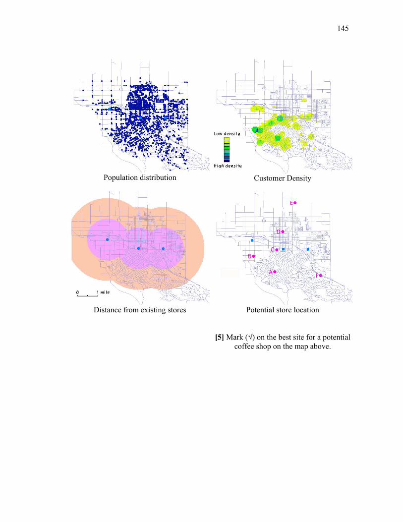
145
Population distribution
Customer Density
Distance from existing stores Potential store location
[5] Mark (√) on the best site for a potential
coffee shop on the map above.

146
Direction: Imagine that you are standing and looking in the direction of the red (or green) arrow. Among 6 photos (A~F) on the next page, which photo most closely represents what you would see? Mark (√) on your answer [Question 6-7]
(A) (B) (C) (D) (E) (F) [6] Red Arrow [7] Green Arrow
Question 6 and 7 were adapted from personal homepage of J. Ryu (2005)

147
(A) (B)
(C) (D)
(E) (F)
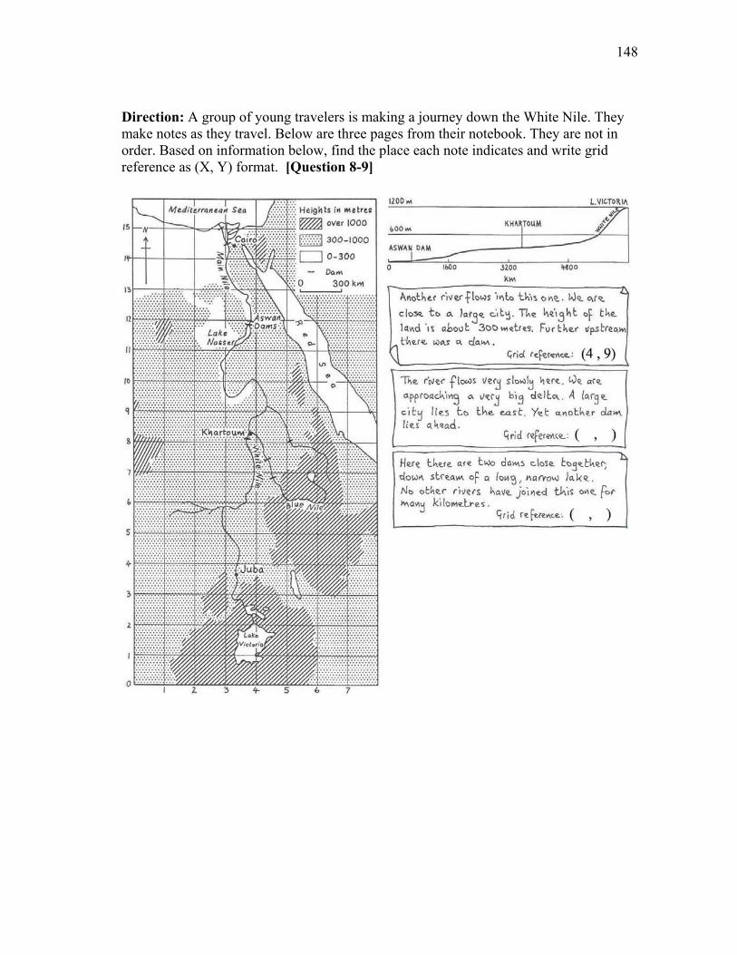
148
Direction: A group of young travelers is making a journey down the White Nile. They make notes as they travel. Below are three pages from their notebook. They are not in order. Based on information below, find the place each note indicates and write grid reference as (X, Y) format. [Question 8-9]
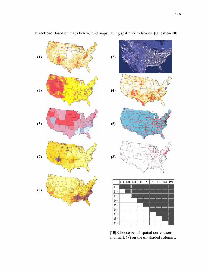
149
Direction: Based on maps below, find maps having spatial correlations. [Question 10]
(1)
(2)
(3)
(4)
(5)
(6)
(7)
(8)
(9)
[10] Choose best 5 spatial correlations and mark (√) on the un-shaded columns.
(1) (2) (3) (4) (5) (6) (7) (8) (9)(1) (2) (3) (4) (5) (6) (7) (8) (9)

150
Direction: The values below are indicating elevation of each point. Based on the elevation data, create contour lines. The contour interval should be 50 feet. The lowest contour line is 400 feet. In this way your contour intervals should run 400, 450, 500… [Question 11]

151
Direction: Spatial information can be displayed based on Point, Line(Arc), Area(Polygon), and Raster(lattice). Based on the sample question below, classify the following spatial data. [Question 12-17]
Point
Line (Arc)
Area (Polygon)
Raster (lattice)
[Sample Question]
[√] Point [√] Line [ ] Area [ ] Raster
[12]
[13]
Soil map
[14]
Elevation [15] River channels and their basins in Brazos County. [16] Locations of weather stations in Harris County. [17] Texas A&M University shuttle bus route in College Station.
Please mark (√) on your answer Point Line Area Raster
[12] [ ] [ ] [ ] [ ] [13] [ ] [ ] [ ] [ ] [14] [ ] [ ] [ ] [ ] [15] [ ] [ ] [ ] [ ] [16] [ ] [ ] [ ] [ ] [17] [ ] [ ] [ ] [ ]

152
Post-Test
Personal Information 1. Name: 2. Major: 3. Freshman / Sophomore / Junior / Senior / Graduate 4. Gender: M / F 5. Have you ever taken a GIS course? : Yes / No
Spatial skills test
a. If you “Yes”, which GIS course? Geog 332 (Thematic Cartography) Geog 361 (Remote Sensing in Geosciences) Geog 390 (Principles of Geographic Information Systems) Geog 475 (Advanced Geographic Information Systems) Others ( )

153
Direction: Solve the following questions based on the example below. Please mark (√) an answer [Question 1-2]
[Example]
[1]
[2]

154
Direction: Based on figures below, solve the following questions. Please mark (√) an answer [Question 3-4]
(A) (B) (C) (D)
[3] (not B) and D
( ) ( ) ( ) ( ) ( )
[4] A and B and C
( ) ( ) ( ) ( ) ( )

155
Direction: Find the best location for a flood management facility based on the following conditions. [Question 5]
• Possible site for a flood management facility should be within 60 ft of an existing electric line.
• Possible site for a flood management facility should be located less than 220 elevation level.
• Possible site for a flood management facility should be located in State Park or Public Land.
Land use
Elevation (feet)
60 feet from electric line
Potential facility location
[5] Mark [√] on the best site for the flood management facility on the map above.

156
Direction: Imagine that you are standing and looking in the direction of the red (or green) arrow. Among 6 photos (A~F) on the next page, which photo most closely represents what you would see? Mark (√) on your answer [Question 6-7]
(A) (B) (C) (D) (E) (F) [6] Red Arrow [7] Green Arrow

157
(A) (B)
(C) (D)
(E) (F)
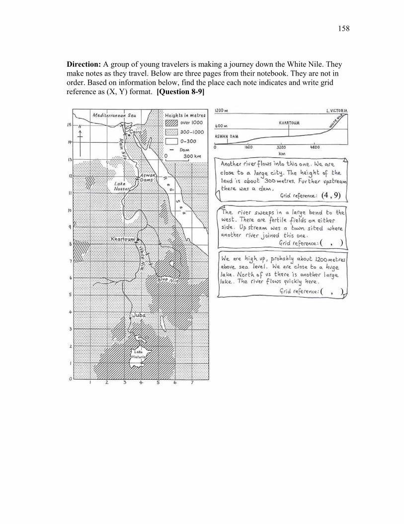
158
Direction: A group of young travelers is making a journey down the White Nile. They make notes as they travel. Below are three pages from their notebook. They are not in order. Based on information below, find the place each note indicates and write grid reference as (X, Y) format. [Question 8-9]
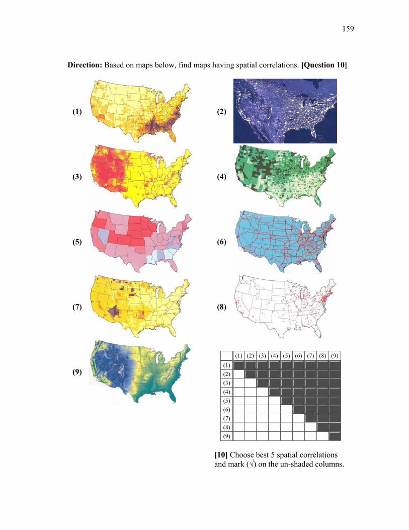
159
Direction: Based on maps below, find maps having spatial correlations. [Question 10]
(1)
(2)
(3)
(4)
(5)
(6)
(7)
(8)
(9)
[10] Choose best 5 spatial correlations and mark (√) on the un-shaded columns.
(1) (2) (3) (4) (5) (6) (7) (8) (9)(1) (2) (3) (4) (5) (6) (7) (8) (9)

160
Direction: The values below are indicating elevation of each point. Based on the elevation data, create contour lines. The contour interval should be 50 feet. The lowest contour line is 400 feet. In this way your contour intervals should run 400, 450, 500… [Question 11]
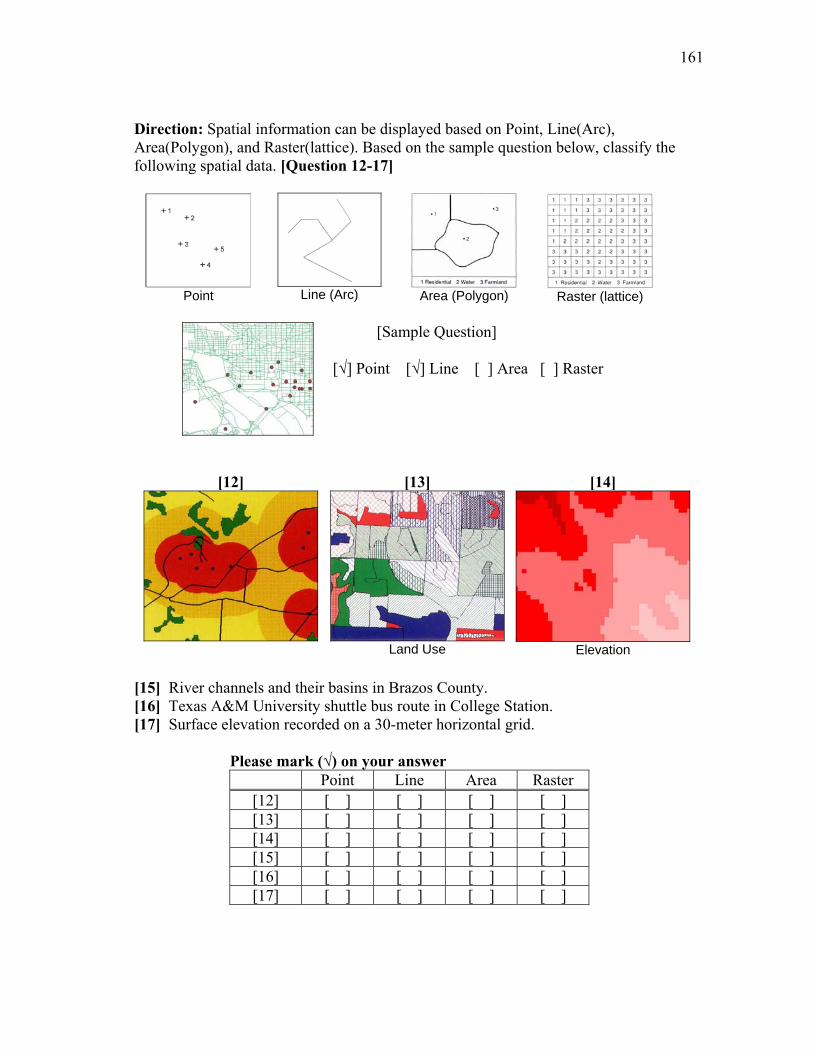
161
Direction: Spatial information can be displayed based on Point, Line(Arc), Area(Polygon), and Raster(lattice). Based on the sample question below, classify the following spatial data. [Question 12-17]
Point
Line (Arc)
Area (Polygon)
Raster (lattice)
[Sample Question]
[√] Point [√] Line [ ] Area [ ] Raster
[12]
[13]
Land Use
[14]
Elevation [15] River channels and their basins in Brazos County. [16] Texas A&M University shuttle bus route in College Station. [17] Surface elevation recorded on a 30-meter horizontal grid.
Please mark (√) on your answer Point Line Area Raster
[12] [ ] [ ] [ ] [ ] [13] [ ] [ ] [ ] [ ] [14] [ ] [ ] [ ] [ ] [15] [ ] [ ] [ ] [ ] [16] [ ] [ ] [ ] [ ] [17] [ ] [ ] [ ] [ ]
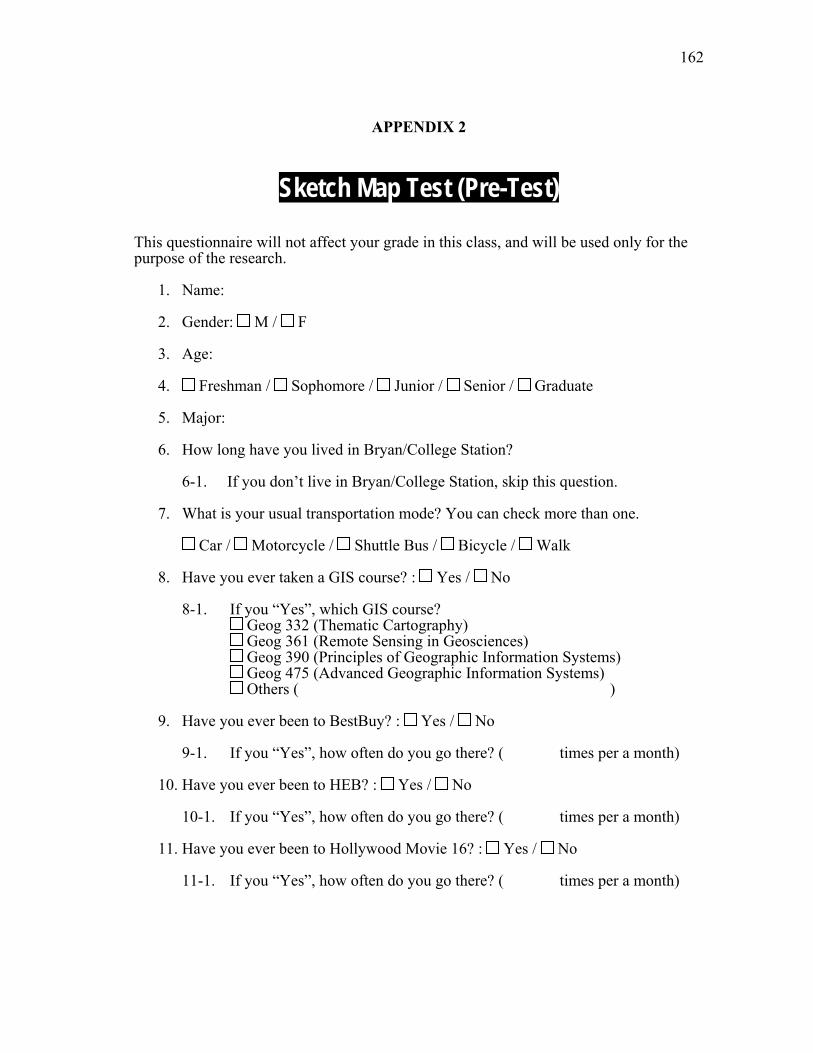
162
APPENDIX 2
Sketch Map Test (Pre-Test) This questionnaire will not affect your grade in this class, and will be used only for the purpose of the research.
1. Name: 2. Gender: M / F
3. Age:
4. Freshman / Sophomore / Junior / Senior / Graduate
5. Major:
6. How long have you lived in Bryan/College Station?
6-1. If you don’t live in Bryan/College Station, skip this question.
7. What is your usual transportation mode? You can check more than one.
Car / Motorcycle / Shuttle Bus / Bicycle / Walk
8. Have you ever taken a GIS course? : Yes / No
8-1. If you “Yes”, which GIS course? Geog 332 (Thematic Cartography) Geog 361 (Remote Sensing in Geosciences) Geog 390 (Principles of Geographic Information Systems) Geog 475 (Advanced Geographic Information Systems) Others ( )
9. Have you ever been to BestBuy? : Yes / No
9-1. If you “Yes”, how often do you go there? ( times per a month)
10. Have you ever been to HEB? : Yes / No
10-1. If you “Yes”, how often do you go there? ( times per a month)
11. Have you ever been to Hollywood Movie 16? : Yes / No
11-1. If you “Yes”, how often do you go there? ( times per a month)

163
A fr
iend
of y
ours
is c
omin
g to
vis
it yo
u in
Col
lege
Sta
tion.
Unf
ortu
nate
ly y
ou c
anno
t sho
w h
im/h
er a
roun
d to
wn.
Dra
w a
m
ap to
hel
p yo
ur fr
iend
find
som
e us
eful
pla
ces.
You
r map
shou
ld in
clud
e th
e O
&M
bui
ldin
g, B
est B
uy, H
EB, a
nd
Hol
lyw
ood
mov
ie16
.Sho
was
muc
has
deta
ilas
you
can.
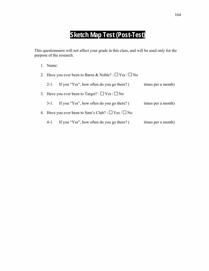
164
Sketch Map Test (Post-Test) This questionnaire will not affect your grade in this class, and will be used only for the purpose of the research.
1. Name: 2. Have you ever been to Barns & Noble? : Yes / No
2-1. If you “Yes”, how often do you go there? ( times per a month)
3. Have you ever been to Target? : Yes / No
3-1. If you “Yes”, how often do you go there? ( times per a month)
4. Have you ever been to Sam’s Club? : Yes / No
4-1. If you “Yes”, how often do you go there? ( times per a month)

165
A fr
iend
of y
ours
is c
omin
g to
vis
it yo
u in
Col
lege
Sta
tion.
Unf
ortu
nate
ly y
ou c
anno
t sho
w h
im/h
er a
roun
d to
wn.
Dra
w a
m
ap to
hel
p yo
ur fr
iend
find
som
e us
eful
pla
ces.
You
r map
shou
ld in
clud
e th
e O
&M
bui
ldin
g, B
arns
& N
oble
s, Ta
rget
, an
dSa
m’s
Clu
b.Sh
owas
muc
has
deta
ilas
you
can.
166
VITA
Jong Won Lee 1710 16th Street NW
Washington, DC 20009-3198
EDUCATION HISTORY
Ph.D. Geography Texas A&M University, College Station, Texas. May 2005
M.A. Geography Education
Seoul National University, Seoul, February 2000
B.A. Geography Education Seoul National University, Seoul, August 1997
EMPLOYMENT HISTORY
Education Fellow: Association of American Geographers, Washington DC, May 2005 – Graduate Assistant Lecturer: Department of Geography, Texas A&M University, College Station, Texas, Fall 2004 – Spring 2005
Graduate Teaching Assistant: Department of Geography, Texas A&M University, College Station, Texas, Fall 2002 – Spring 2004
Researcher: Korea Institute of Curriculum and Evaluation, Seoul, 2000 – 2001