Effect of Design Parameters on the Mass of a Variable-spanMorphing Wing Based on Finite Element Structural Analysis

and Optimization

Pedro D.R. Santosa,∗, Diogo B. Sousaa, Pedro V. Gamboaa, Yifan Zhaob

aDepartment of Aerospace Sciences, Faculty of Engineering, University of Beira Interior, PortugalbThrough life Engineering Services Centre, Cranfield University, United Kingdom

Abstract

In the past years, the development of morphing wing technologies has received a

great deal of interest from the scientific community. These technologies potentially

enable an increase in aircraft efficiency by changing the wing shape, thus allowing

the aircraft to fly near its optimal performance point at different flight conditions.

However, these technologies often present an undesired mass increase due to their

inherent complexity. Therefore, the aim of the current work is to ascertain the

influence of geometrical and inertial parameters on the structural mass of a Variable-

span Wing (VSW). The structural mass prediction is based on a parametric study.

A minimum mass optimization problem with stiffness and strength constraints is

implemented and solved, being the design variables structural thicknesses and widths,

using a parametric Finite Element Model (FEM) of the wing. The study is done for

a conventional fixed wing and the VSW, which are then combined to ascertain the

VSW mass increment, i.e., the mass penalization of the adopted morphing concept.

Polynomials are found to produce good approximations of the wing mass. The effects

of the various VSW design parameters in the structural mass are discussed. On one

hand, it was found that the span and chord have the highest impact in the wing mass.

On the other hand, the VSW to fixed wing mass ratio proved that the influence of

span variation ratio in the wing mass is not trivial. It is found that the mass increase

does not grow proportionally with span variation ratio increase and that for each

combination of span and chord, exists a span variation ratio that minimizes the mass

penalty. In the future, the developed polynomials could be used to create a mass

∗Corresponding author at: Department of Aerospace Sciences, Faculty of Engineering, Universityof Beira Interior, Portugal

Email address: p_daniel_santos@hotmail.com (Pedro D.R. Santos)

prediction model to aid the design of morphing wings during the conceptual design

phase.

Keywords: Morphing Wing, Variable-span Wing, Telescopic Wing, Optimization,

Finite Element Model, Parametric Study, Composite Material Structure,

Multivariable Polynomial Fitting

1. Introduction

Mass control, namely the process by which the lightest possible aeroplane is de-

rived within the constraints of the design criteria [1], is an essential part of the design

process of any aerospace vehicle. Accurate estimations of aircraft mass are vital in

the early stages of an aircraft design process. They drive all the major choices in

configuration and layout as well as being the main foundation of performance predic-

tions. Mass estimation in aircraft design is very challenging due to the high number

of variables involved in the creation of an accurate mass model, the numerous re-

lationships between them and the high degree of uncertainty associated with the

problem itself.

Morphing wing technologies require the concurrent development of design and

optimization strategies to expedite overall development of these systems. The devel-

opment of robust morphing wing sizing codes to be used during conceptual design

tasks is of major importance, since it enables studies of the operational benefits and

provide a methodological basis for future morphing aircraft sizing codes. However,

such tools need accurate mass predictions for the major components, including the

morphing wings. Therefore, morphing technologies will only be considered in new air-

craft development, if mass predictions with sufficient accuracy are available. Simple

and sufficiently accurate mass prediction methods for designing morphing wings at

the conceptual design phases are rare. Therefore, the benefits that one morphing

strategy can offer over another or even over a conventional fixed wing are thus quite

difficult to assess without resorting to detailed time consuming Finite Element Model

(FEM), normally only performed at the detailed design phase.

Most of the existing mass estimation models available in the literature can be clas-

sified into two main categories: semi-empirical and finite element [2]. Semi-empirical

models are based on data from similar existing aircraft. Therefore, the robustness

2

of these models depends on the similarities: size, configuration, and technology (sys-

tems, structural efficiency, and materials), between the aircraft under study and the

aircraft that have been used in the derivation process of these models [3]. In the

case of morphing wings, little information is currently available to substantiate such

a wing mass prediction and thus, the sizing results would be unfounded. On the

other hand, FEMs are not suitable to be used during the conceptual and preliminary

design phases, since they require detailed knowledge of the internal geometry and

aerodynamics that are usually not available early in the design process [4]. Thus, it

is desirable to formulate a model based on FEM analyses, to capture the structural

trends, but without the complexity posed by these methods.

Various studies have been performed in mass models for conceptual design of

conventional wings. Some developed wing mass estimation models for commercial

and transport aircraft [2, 5] and others for more unconventional configurations, such

as nonplannar configurations [6, 3, 7] or high speed transport [8]. However, very few

studies have focused on morphing wings.

Frommer and Crossley [9] used a technique called photo-morphing. In this tech-

nique, the reference wing mass is computed using a mass model developed for con-

ventional wings, the so called basic mass. Then, this value is corrected for actuation

system mass, using the maximum variation in unique planform area, multiplied by

an actuator specific (in relation to area) mass constant. This metric is indicative of

the wing planform that needs to be moved when changing from one shape to another.

Although the photo-morphing is simple to implement, it is very limiting, since there

may be no skin materials or actuation strategy to achieve some of the represented

shape changes. Additionally, the actuator specific mass constant is difficult or even

impossible to derive for some morphing systems.

Probably, the most significant study was performed by Skillen and Crossley

[10, 11], where they developed a wing mass model, considering the variation of span,

chord and sweep. FEM analyses, based on equivalent box-beam models or shell type

structures, were used to estimate the mass for a sufficient number of combinations

and then a least square regression was used to approximate the wing mass. Val-

idation examples were provided for chord and variable sweep morphing wings. No

details about the span variation methodology were given. The shape variation con-

3

sidered clearly required the use of high strainable skins, but they were not formally

addressed in the FEM, potently resulting in erroneous mass estimations. Moreover,

the actuation system was modelled using simplified hydraulic actuators, not being

considered other types of actuators that could yield better results, specially for small

sized Remotely Piloted Aircraft Systems (RPAS).

From what has been presented, methods to predict wing mass of morphing wings

are limited and scarce. Morphing wings can have an undesired mass increase due to

their inherent complexity both in the load carrying structure and in the actuation

systems. This can potentially limit or even negate any performance benefits, depend-

ing on the intended flight mission and/or aeroplane type. However, mass estimation

of morphing wings is difficult and very little is known about the impact of wingspan

or wingspan maximum variation, among others, on the mass of the load carrying

structure. Therefore, the present work has two main goals:

• Ascertain the influence of geometrical and inertial parameters on the structural

mass of a Variable-span Wing (VSW) concept with an integrated Trailing Edge

(TE) device;

• Develop mass prediction functions by fitting multivariable polynomial approx-

imations. These can be used, in the future, to create a mass prediction model

of VSWs that could be used during the conceptual design phases.

A total of five parameters were considered, namely, wingspan, wing chord, span

variation ratio, flap chord ratio and aeroplane weight. To achieve this, a minimum

mass optimization problem with stiffness and strength constraints was implemented

and solved for a sufficient number of combinations of the wing parameters, being the

design variables, structural thicknesses and widths. A parametric structural FEM of

the wing was built in APDL and solved in ANSYS®. Concurrently, the same study

was performed for a conventional fixed wing. Using the computed data, mass and

mass ratio functions were created by fitting multivariable polynomials: fixed wing

mass, VSW mass and VSW to fixed wing mass ratio. The latter was used to ascertain

the mass penalty associated with the adopted morphing concept. Additionally, the

effects of various VSW design parameters in the structural mass were inferred and

synthesized.

4

2. Variable-span Wing Concept

2.1. Wing Concept

The morphing wing herein presented relies on a telescopic wing. The layout of

the VSW concept is based on a hollow Inboard Fixed Wing (IFW) that is attached to

the fuselage, inside of which an Outboard Moving Wing (OMW) slides actuated by

an electromechanical mechanism. This concept consists of a two element rectangular

telescopic wing containing a variable camber TE that starts next to the fuselage and

extends in the spanwise direction up to the region where the moving element of the

wing retracts into. The VSW does not possess ailerons, allowing for structural simpli-

city and improved aerodynamic performance. Rolling moments could be effectively

controlled by asymmetrical wingspan variation.

Figure 1 shows a planform conceptual view of the VSW, where the main planform

parameter names are identified for easier description. The VSW has some differenti-

(a) (b)

Figure 1: VSW conceptual planform view: (a) fully retracted and (b) fully extended configuration,with geometrical parameters identified.

ating factors, namely the use of a canted wingtip and a morphing flap. The wingtip

is intended to provide additional lateral-directional stability. In fact, it creates an

effective dihedral angle, without changing the telescopic sections of the wing, thus,

decreasing the structural and actuation system complexity that would result from

non-flat wing sections. Additionally, the wingtip increases the overall aerodynamic

efficiency. Finally, the addition of the morphing flap enables camber changes, result-

ing in an increase in lift-to-drag ratio at different flight lift coefficients.

Both IFW and OMW wing panels have the design constraint of keeping chord

and aerofoil geometry constants along each panel span, enabling proper fitting and

support of the OMW. Observing Fig.1 one can see that the IFW length is denoted

by lIFW , the OMW length by lOMW , the tip length by ltip and the flap length by

lflap. The lvar parameter refers to the span length that is variable as a result of the

5

movement of the OMW. There are two regions of contact that aid the load transfer

from the OMW to the IFW: lover1 and lover2. The former is the innermost region

and is responsible for carrying the majority of the bending and torsional moments of

the OMW. The latter corresponds to the outermost contact region, being responsible

for providing stability in the chordwise direction. There is an additional length

parameter that takes into account the fuselage length, called lfus. Finally, IFW,

OMW, flap and tip chords are designated as cIFW , cOMW , cflap and ctip, respectively.

The shape and size of the VSW reference design was obtained through an in-

house computational constrained aerodynamic shape optimization code, aimed at

determining the wing mean chord and span values that minimize its drag for the

specified mission profile. A detailed description of the aerodynamic optimization

procedure is given in [12]. Along with the optimization procedure, two geometrically

compatible aerofoils were provided in a way that the OMW slides inside the IFW. The

method employed to geometrically offset the aerofoils and determine its aerodynamic

performance is fully explained in [13].

2.2. Structural Concept and Materials

In principle, morphing wings tend to be heavier than conventional fixed wings due

to increased structural and actuation complexity. Therefore, the structure should be

designed and materials selected in such a way that sufficiently light wing components

are attained. This facilitates integration into a realistic application while maintaining

rigidity to carry flight loads. Therefore, the VSW uses a semi-monocoque structural

concept, which consists in a stressed skin construction that carries shear loads, rein-

forced by multiple spars to carry bending and torsion moments.

Figure 2 shows a schematic of the IFW and OMW wing cross-sections, where the

main sectional parameters are identified to facilitate the description.

(a) (b)

Figure 2: VSW cross-section view with sectional parameters identified: (a) inboard fixed wing and(b) outboard moving wing sections.

6

Observing Fig.2, it is visible that both sections are composed by a composite

sandwich made up with a foam core and two plies of bidirectional laminated carbon-

epoxy composite. The fibres of the laminate are orientated at an angle of ± 45°. The

four unidirectional pultruded carbon-epoxy composite spar caps are integrated into

the skin, two in the upper surface and the other two in the lower surface. The two

frontal spar caps are located in the thicker aerofoil section (30% of the local chord),

while the two rear spar caps are located at a chord ratio dictated by the flap chord

(cflap).

Looking at the IFW section (Fig.2(a)), only one web (vertical element of the wing-

box) is visible and it does not extend the full length. Instead, it is interrupted at the

end of the flap position (lfus + lflap) from its root, in order to allow the OMW to

retract into the IFW. Due to this constraint, no internal ribs can be used. Therefore,

chordwise reinforcements made with unidirectional laminated carbon-epoxy compos-

ite are applied in three critical sections: beginning/end of the flap and IFW tip.

In Fig.2(b) it can be seen that the OMW has two webs. They extend from

the component’s root to the end of the rectangular portion (beginning of wing tip).

Similar to the IFW, the two frontal spar caps and webs are located in the thicker

aerofoil section (30% of the local chord), while the two rear spar caps and webs are

located in a chord ratio dictated by the flap chord (cflap). There are no chordwise

reinforcements in the OMW, since four internal ribs are used: OMW root and lover2

location, end of the rectangular portion and end of wingtip.

Several sectional parameters are identified in Fig.2: tlam and tlam,web denote the

laminate thicknesses of the skin contour and web; tfoam and tfoam,web denote the

foam core thicknesses of the skin contour and web; and wsc denotes the width of the

spar caps. The subscripts IFW and OMW are added to the mentioned terminology,

in order to differentiate the parameters of the former and latter sections.

The VSW is made with three materials: carbon-fibre fabric with epoxy for the

faces of the sandwich; PVC foam (Airex® C70.90) for the core of the sandwich and

internal ribs; and pultruded unidirectional carbon-fibre with epoxy for the spar caps

(vDijk high-strength pultrusions).

Material properties of the PVC foam and pultruded unidirectional carbon-fibre

were obtained from the manufacturer’s datasheet. The properties of the sandwich

7

faces are assumed for a hand lay-up procedure with vacuum curing [14].

The properties of these materials are presented in Table 1. The pultruded carbon

fibre and woven carbon/epoxy are formulated as orthotropic materials and the PVC

foam is considered to be an isotropic material. Note that subscripts 1 and 2 denote the

direction of the fibre and perpendicular to the fibre, respectively (where applicable).

Table 1: Material properties used in the VSW parametric study.

PropertyWoven

carbon/epoxyPultruded

carbon/epoxy Airex® C70.90

ρ, kg/m3 1500 1600 100E1, GPa 46 105 0.084E2, GPa 46 7.5 -G12, GPa 3.25 3.75 0.040

ν12 0.1 0.3 0.05Ftu1, MPa 600 1500 2.7Ftu2, MPa 600 50 -Fcu1, MPa 570 1200 2Fcu2, MPa 570 250 -S12, MPa 90 70 1.7

3. Parametric Study Methodology

The most common approach to developing fixed-wing mass predictions is centred

on the idea that a large database of wing masses and their associated geometry

already exists through previous developed aircraft. Direct application of the above

approach is not possible for morphing wing components because an adequate set

of aircraft data does not exist. The approach used here is to develop a wing mass

database and develop an equation that approximates this database. Using a Design

of Experiments (DOE) to define a set of morphing wings with various shapes, rep-

resentative FEMs were developed for each wing in the database and then sized to

give a corresponding mass estimate. These data can then be approximated using an

appropriate basis equation using a least squares regression technique resulting in the

morphing wing mass equation. Only the structural mass was considered here. The

various aspects of this procedure are described in detail in the following sections.

The VSW presented in detail in the previous section serves as a basis to perform

the parametric study with a double purpose. On one hand, it allows the study of

the influence of a set of geometrical and inertial parameters on the structural mass

8

of the VSW. On the other hand, as already mentioned, it allows the creation of the

mass database, needed to create the approximation to predict the structural mass of

the VSW. A total of five parameters were selected to perform the study. These are

1. b - wingspan in fully extended configuration;

2. cIFW - inboard fixed wing chord;

3. lvar - wing variable-span (VS) ratio (with respect to semi-span);

4. cflap - flap chord ratio (with respect to cIFW );

5. W - aeroplane Maximum Takeoff Weight (MTOW).

The first four parameters are called the wing geometrical base parameters, since

all the other wing dimensions are derived from those. Parameters one and two are

illustrated in Fig.1. Parameters three and four, lvar and cflap, are nondimensionalized

versions of lvar and cflap, using the semi-span and the IFW chord, respectively. The

fifth mentioned parameter, the aeroplane MTOW, W , was included in order to size

the wings with different loading conditions and is used to compute the maximum

load factor, using the CS-VLA regulation (described in Section 3.4).

For each set of parameters a minimum mass optimization problem with stiffness

and strength constraints was implemented and solved, being the design variables

structural thicknesses and widths. The optimization and structural FEM of the wing

were developed in ANSYS® APDL.

The characteristics of an in-house developed RPAS were used to define a refer-

ence wing configuration. Those characteristics are: MTOW of 150 N; IFW chord of

0.257 m; span of 3.554 m in the fully extended configuration and a span of 3.104 m

in the fully retracted configuration, giving a span variation to span ratio of 0.25.

3.1. Optimization

The optimization was carried out for each wing configuration, with the purpose

of minimizing wing mass and, at the same time, ensure that each wing supports the

prescribed loading. ANSYS® Mechanical APDL internal optimization facilities were

used to carry out the optimization. The first order method was used, since it is the

most accurate method available [15]. This method of optimization computes and

uses derivative information. The constrained problem statement is transformed into

9

an unconstrained one via penalty functions. Derivatives are formed for the objective

function and the state variable penalty functions, using central finite differences, lead-

ing to a search direction in the design space. Various steepest descent and conjugate

direction searches are performed during each iteration until convergence is reached.

Each iteration is composed of multiple sub-iterations that include search direction

and gradient computations [15].

The Design Variables (DV) adopted in the current study were: IFW and OMW

laminate thicknesses, tlam,IFW and tlam,OMW , and IFW and OMW spar cap widths,

wsc,IFW and wsc,OMW (see Fig.2). Maximum bounds of laminate thicknesses were

chosen based on the limitation of the thin shell element derivation assumptions, since

shells elements can not have a radius of curvature to thickness ratio ≤ 0.5. Notice

that these upper bounds are only used to improve optimization stability and they do

not have an impact on the final optimized values. The maximum spar cap widths

were dictated by geometric constraints, i.e., maximum width that avoids mutual

intersection. In the IFW, this is a function of the local and flap chord. In the OMW,

it is only a function of the local chord.

Three constraint functions were adopted: maximum tip deflection and rotation,

and ratio of elements that display failure. The tip deflection, wtip, was limited to

2.5% of the span (b) and the tip rotation, θtip, to be between -0.6 and 0.6°. These

constraints were necessary to allow an even slide of the two wing components. In

fact, if the tip displacement or rotation were too large, the VSW mechanism could

eventually jam, compromising system integrity and functionality. These bounds were

derived from past experience [14]. Additionally, a failure criterion constraint was used

to detect structural failure of the wing. The inverse of Tsai-Wu strength ratio index

failure criterion was used. In the current implementation, the ratio of the failed

elements, SRTW , was imposed to be less than 0.1% of the total number of elements,

rather than imposing that all elements do not display failure. This is due to the

possibility of existing small areas with failed elements, that could be easily solved

using local reinforcements. Since the current study is appropriate for the conceptual

design phases, these small areas should not drive the overall design.

10

In short, the optimization problem can be written as

Minimize: mwing = f(wsc,IFW , tlam,IFW ,

wsc,OMW , tlam,OMW )

Subjected to: wsc,IFW,min < wsc,IFW < wsc,IFW,max

wsc,OMW,min < wsc,OMW < wsc,OMW,max

tlam,IFW,min < tlam,IFW < tlam,IFW,max

tlam,OMW,min < tlam,OMW < tlam,OMW,max

wtip < 0.025 b

|θtip|< 0.6◦

SRTW < 0.001

(1)

Figure 3 summarizes the general flow of steps in the developed parametric design

script.

Figure 3: Parametric design script flowchart.

Observing Fig.3, one can divide the work-flow in the following steps:

1. Variable initialization: variables are initialize using the user defined parameters

(geometrical base parameters, aeroplane MTOWs, constraint function limits,

among others).

2. Parameters calculation: Step 2 signals the start of the DOE loop. Design

dependent parameters are calculated using equations defined in the geometric

scaling (described in Section 3.5). Additionally, maximum span variation for

the configuration under evaluation is computed.

3. Search feasible solution: This step is critical to enhance the stability and conver-

gence time of the optimization procedure. The parametric study base variables

and a first guess of the design variables are used to evaluate the feasibility of the

11

wing structure. A solution is considered feasible if it meets all the constraint

functions. Wing deformations and stresses are computed using the FEM script

(subject of the next section). This first guess is a user prescribed value if it

is the first run or the previous optimized values if otherwise. Two loops are

used: a coarser loop to quickly find design values that satisfy the constraints

and a finer loop to refine these values. In the coarser loop a multiplier is used,

which starts at 1 and increases by 1 each loop, changing the values of the design

variables until a feasible solution is found. In the finer loop, the same technique

is used 8 times with decreasing multipliers (0.5, 0.25, 0.125...).

4. Establish base solution: The optimization procedure requires a starting solution

to be performed. This solution is done using the design variables determined

in the previous step.

5. Optimization initialization: Here the optimization problem is defined, namely

design variables, objective and constraint functions, and optimization method.

6. Optimization: In step 6, ANSYS® internal optimization facilities are started.

The optimization continues until convergence is achieved by comparing the

current iteration design set to the previous set and the best set, using an ob-

jective function tolerance (chosen by the user), or until the maximum number

of iterations is reached [15].

7. Write results: The main outputs of the optimization are written, namely: final

values of the optimization variables, tip deflection and rotation, fraction of

elements that display failure, among others.

8. DOE check: Evaluate if all the values in the DOE were already analyzed. If

the check is true the loop ends. If the check is false the script continues to step

2 and proceeds to the evaluation of the next wing configuration.

3.2. Finite Element Analysis

The numerical model of the VSW wing was developed using the ANSYS® Para-

metric Design Language (APDL) [16] with shell elements according to the base geo-

metrical variables and design variables. The APDL script handles geometry creation,

material definition, section properties, meshing, analysis and post-processing. The

developed script allows the computation of a static solution (deformations, rotations

12

and stresses) using small deformations. Due to computational resource optimization,

SHELL281 element was used to discretize the surfaces. This element is an eight-node

element suitable for analysing thin to moderately-thick shell structures. It has a total

of six degrees of freedom at each node: translations in the x, y and z directions, and

rotations about the x, y and z-axes. The element is well-suited for linear, large

rotation, and/or large strain nonlinear applications.

The IFW sandwich skin was modelled with three layers built as offset surfaces

from the aerofoil contour according to their own thickness. These three layers consti-

tute the carbon/epoxy faces and foam core. In the locations of the embedded spar,

the foam layer was replaced with rectangular cross-section unidirectional pultruded

carbon/epoxy rods. Likewise, the OMW was discretized using the same approach.

The peculiar structure used by the VSW, required the use of contact elements,

in order to correctly model the interface. The contact in the overlapping surfaces

between the IFW and the OMW was modelled with a shell to shell contact using

TARGE170 (target element for 3D geometries surfaces) and CONTA174 (contact

element for 3D shells with mid side nodes). The contact elements were added to

the lover1 and lover2 regions. In order to reduce computational cost, an asymmetric

contact was created. In this type of contact, one surface is designated to be the

target and the other a contact surface. Then, one contact pair is created between

surfaces. Contrary, in the symmetric contact both surfaces are designated as target

and contact, which requires the creation of two contact pairs. Consequently, the

asymmetric contact is more efficient than the symmetric contact. The contact ele-

ments’ behaviour was chosen to be bonded, in order to reduce the computation cost

of each analysis. However, an increase in the local stiffness is to be expected, which

has the effect of underestimating the wing deformations. The bonded contact uses

a Multipoint Constraint (MPC) formulation. MPC uses rigid constraint equations

between the elements on the contact and target faces to model the bonded connec-

tion. The connection locations are determined using the contact element pinball

radius and then the contact elements are replaced with internal constraint equations.

The performed solution was a static analysis, without large deflections and us-

ing the MPC based contact interface. Given these characteristics, the solution was

linear, greatly reducing the computation time for each static analysis. In turn, this

13

improved the robustness of the optimization, since it reduces the possibility of un-

converged solutions. It should be added that since a symmetric wing planform was

assumed, only one wing was modelled. Figure 4 summarizes the general structure of

the developed FEM script.

Compute Wing Dimensions

Create Surface Based Geometry

Define Element Types and Material

Properties

Create and Associate Sections to Surfaces

Define Contacts between IFW/OMW –

MPC Based

Constrain Finite Element Model

Apply Aerodynamic Loading

END

Define Static Analysis

Solve Linear Problem Compute MassPost-process FEM

Results

Compute Maximum Tip Displacement

Compute Maximum Tip

Rotation

Determine Fraction of Failed Elements using “Inverse of

Tsai-Wu Strength Ratio Index Failure Criterion”

Finite Element Analysis

Figure 4: Finite element model flowchart.

3.3. Polynomial Fitting

Several basis functions can be used to approximate the mass of the wings under

study. In the present study, a full quadratic polynomial was used. The general form

of such equation is given by

m({X1:n}) = a0 +

n∑

i=1

aiXi +

n∑

i=1

n∑

j=i

aijXiXj (2)

where, {Xi} represents one of the n parameters within the DOE and aij represent the

unknown coefficients in each of the mass equations. The quadratic approximation

captures both linear and quadratic terms and tends to provide a good approximation

when the design set displays moderate deviations from linear behaviour. Therefore,

it can approximate the wing mass if a non-linear relationship of the wing mass para-

meters is verified. The second order polynomial allows a better study of the effect

on the wing mass produced by each individual parameter, since both linear and two

level interaction relationships between parameters could be identified.

A total of two structural mass and one mass ratio equations were developed: fixed

wing mass, VSW mass and VSW to fixed wing mass ratio. Multivariate polynomials

were then created, mstr,fw, mstr,V SW and mstr,V SW/fixed being a function of the wing

14

parameters in the following form

mstr,fw =f(b, cIFW , cflap,W ) (3)

mstr,V SW =f(b, cIFW , lvar, cflap,W ) (4)

mstr,V SW/fw =f(b, cIFW , lvar, cflap,W ) (5)

where, Eqs.(3), (4) and (5) are functions of the already mentioned parametric study

parameters, with the exception of the first (fixed wing polynomial) that does not

have VS ratio. Notice that Eq.(5) is not a mass equation since it represents the ratio

of VSW mass to fixed wing mass, thus being a non-dimensional quantity.

A mathematical algorithm was applied to find the unknown polynomial coeffi-

cients. The used method is based on an extension to the Granger causality test,

called ERR-causality [17]. The main advantage of the ERR test is that it can be

applied to nonlinear multivariate systems. Furthermore, with the ERR-causality

method it is possible to organize the polynomial terms, in respect to its significance

to the overall solution. Therefore, the complete polynomial model does not have

to be used to provide a good polynomial approximation. The minimum number

of significant terms that adequately fits the dataset is evaluated by calculating the

Sum of Error Reduction Ratio (SERR) values. Using this metric, the final simplified

polynomial can be obtained, by screening the terms that have lower influence in the

dependent variable and eliminating them.

The resulting polynomials were evaluated using goodness of fitting parameters:

coefficient of determination, R2, maximum relative error, maximum absolute error

and Root Mean Squared Error (RMSE). The R2 correlates the computed data with

the predicted data by a square of the sample correlation coefficient, where values near

to one indicate a good fit. RMSE is a fit standard error for regression and estimates

the standard deviation of each data component [18].

After computing the polynomial, it was important to visually validate the results

by plotting the representation of the resulting polynomials with the data points

overlaid for comparison reasons. These plots facilitated final considerations to be

taken about the trends of each parameter on the wing mass. The five independent

variables describe a hypersurface with a six-dimensional representation. As this is

15

not possible to plot, the complete polynomial approximations were reduced to several

polynomials with only two independent variables.

3.4. Loading

The design load cases are important to determine realistic sizes of the wing’s

structural components. These load cases are usually defined by the limits of the V-n

diagram. In fact there may be combinations of bending and torsion moments outside

the corner points which may size individual components. Ideally, the wing structure

would be optimized with respect to all expected loading and operating conditions.

However, this results in an extremely large number of loading conditions. Therefore,

selecting only the critical loading condition should suffice to demonstrate the present

approach.

In general terms, the morphing aircraft is expected to perform a long-endurance

loiter, followed by a high speed dash. The morphing wing would have a high aspect

ratio during loiter to reduce induced drag. During dash, the wing would have a low

aspect ratio. Thus, the maximum speed of the dash wing is significantly higher than

that of the loiter wing. Therefore, each configuration of the morphing wing has its

own V-n diagram and, consequently, each configuration has its own set of design

loads.

To extract the different design loads, the reference baseline VSW was analysed

in three wing configurations: maximum, intermediate and minimum span. For each

configuration, manoeuvre and gust V-n diagrams were computed, using the EASA’s

Certification Specifications for Very Light Aeroplanes, CS-VLA [19] and the RPAS

specifications. From each V-n diagram the critical design points were extracted based

on the maximum load factor which corresponds to the maximum bending moment.

For aeroplanes with low wing loading (W/S), the gust envelope is critical [20].

Therefore, the maximum load factor of the gust diagram was used as design point.

The next paragraphs explain in more detail the rational behind this methodology.

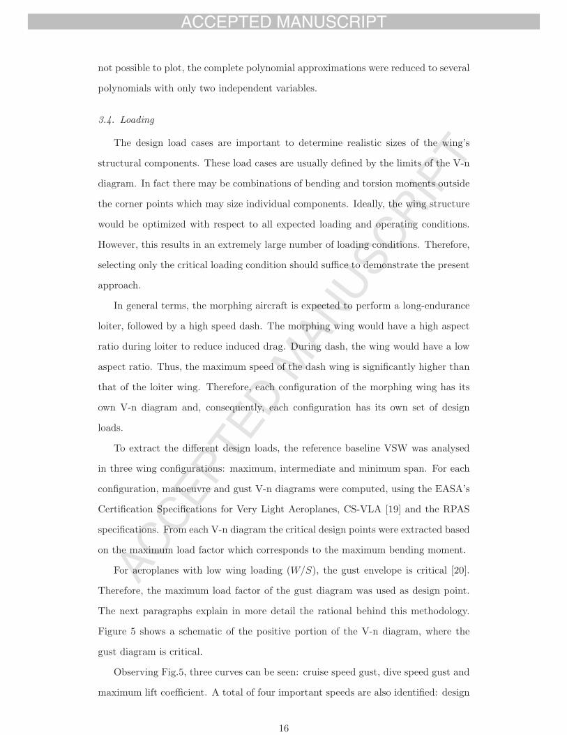
Figure 5 shows a schematic of the positive portion of the V-n diagram, where the

gust diagram is critical.

Observing Fig.5, three curves can be seen: cruise speed gust, dive speed gust and

maximum lift coefficient. A total of four important speeds are also identified: design

16

speed

load

fact

or

Figure 5: Schematic of the positive portion of the V-n diagram, where the gust diagram is critical.

cruise speed, VC , design dive speed, VD, stall speed, Vstall, and design speed, Vdesign.

Referring to CS-VLA norm, the design cruise speed, VC , and the dive speed, VD, are

computed using the following equations

VC = VC,min =2.4√W/S (6)

VD = VD,min =1.25VC (7)

being, W the aircraft weight and S the wing area. Analysing Eq.(6), one concludes

that cruise speed is a function of the wing loading.

The cruise and dive gust curves are computed, as functions of speed, according

to the CS-VLA norm, using the following equations

nVC= 1 +

ρair V CLα Kg Vg,C

2W/S(8)

nVD= 1 +

ρair V CLα Kg Vg,D

2W/S(9)

where Kg is the gust alleviation factor, CLα is the wing lift curve slope, Vg,C and

Vg,D are the gust vertical speeds in cruise and dive conditions, respectively. Note that

the gust vertical speeds are constant values (given in CS-VLA). The gust alleviation

factor and the aeroplane mass ratio, μg are introduced to correct for dynamic effects

in the aircraft pitching and vertical motion and the time lag during which lift is

building. They are computed from

Kg = 0.88μg

5.3 + μgwith μg =

2W

ρair cIFW CLαS(10)

The lift curve slope is estimated from the aerofoil lift curve slope, considering an

17

inviscid, incompressible flow over a wing with general planform [21]. Thus

CLα =Clα

1 + Clα/(π AR)(1 + τ)(11)

where, Clα is the aerofoil lift curve slope, AR is the wing aspect ratio and τ is a

function of the wing planform. In the current work, although the wing planform is

not elliptic, the lift distribution is assumed to have an elliptic shape. Therefore, τ

can be neglected.

The stall load factor is computed using the definition of lift for maximum lift

coefficient. Thus

nCL,max=

0.5 ρair V2 S CL,max

W(12)

From Fig.5, one can see that, for low speeds, the nCL,maxcurve is the limiting load

factor. When the cruise speed is reached, the load factor reduces linearly between the

two gust curves. The maximum gust load factor speed is found in the intersection

between nVCand nVD

curves and nCL,maxcurves, denoted by Vdesign. Therefore

nVC+

nVD− nVC

VD − VC(Vdesign − VC) =

0.5 ρair V2design S CL,max

W(13)

Solving Eq.(13) for Vdesign, yields the speed for the maximum gust load factor.

The design load factor can now be determined by substituting the computed speed

in the load factor for the maximum lift coefficient. Thus

ndesign =0.5 ρair V

2design S CL,max

W(14)

After computation of the design load factor, the design lift force can be readily

computed from

Ldesign = ndesignW (15)

Drag and pitching moment can now be computed. The drag was determined

using the lift-to-drag ratio of the baseline wing. This quantity was corrected using

the aspect ratio, if a different wing is considered. Therefore

Ddesign =Ldesign

(L/D)blw AR/ARblw(16)

18

where, (L/D)blw and ARblw are the lift-to-drag ratio and aspect ratio of the baseline

wing, respectively.

The pitching moment is computed from the baseline wing pitching moment coef-

ficient and the design speed. Thus

Mdesign = 0.5 ρair V2design S cIFW CM,blw (17)

being CM,blw the pitching moment coefficient of the baseline wing. The pitching

moment coefficient used is an average value in the studied range of lift coefficients of

the baseline wing. It was assumed constant for all studied wing configurations.

The lift was considered to have an elliptic distribution, applied along the span

at 25% chord position. Both drag and pitching moment distributions were assumed

uniform along the wingspan. Lift and drag forces are perpendicular and parallel,

respectively, to the free stream direction. However, since the effect of the AOA was

not considered, they are assumed to be perpendicular and parallel to the wing chord

line, respectively. Therefore, lift force is the vertical force, FV , and the drag force is

the horizontal force, FH .

Finally, in order to better represent the load distributions along the chord, the

initial force system of one vertical and horizontal force, applied at 25% of the wing

chord, and a torsion moment about this same point, was substituted by two vertical

forces applied at the fore and aft wing-box webs and four horizontal forces applied

at each spar cap corner, as shown in Fig.6.

Figure 6: Equivalent force system of the VSW parametric study (FV is the vertical force, FH thehorizontal force and M the pitching moment).

19

From the force and moment equilibrium, forces FV,1 and FV,2 are found to be

FV,1 =FV − M − 0.25cFV + x1cFV

c(x1 − x2)(18)

FV,2 =M − 0.25cFV + x1cFV

c(x1 − x2)(19)

where, x1 and x2 are the ratios of the fore and aft spar positions to the chord length

of the VSW. In the studied case, the fore ratio is 0.3 and the aft ratio is dependent

on the flap chord (1− cflap).

The fore vertical load was distributed along the frontal web of the wing, the aft

vertical force was distributed along the rear web of the wing and the horizontal force

was equally distributed by the four spar caps.

3.5. Geometric Scaling

In the parametric study, different wing geometric configurations were used. Thus,

there was a need to create geometric mathematical relations between the different

used parameters. In order to perform the scaling, a baseline or reference wing was

used, being its dimensions designated using the subscript blw, where “bl” stands

for baseline and “w” to wing. The geometric scaling can be divided into spanwise,

chordwise and sectional parameters. As the names implies, the former denotes para-

meters in the spanwise direction and the second in the chordwise direction. The

latter denotes mathematical relations of the section thicknesses and widths.

3.5.1. Spanwise Formulas

In the spanwise scaling, the important input parameters are the wingspan, b,

and the VS ratio, lvar. The innermost overlap between the IFW and OMW, lover1

is scaled using the OMW exposed area (moving part) and tip area, as well as the

y centroid of the same sections. In fact, with increasing lvar the bending moment

in the contact surface location increases and section centroid location moves away

from the wing’s root. Consequently, lover1 needs to increase to allow a smooth load

transfer. The derived mathematical relation is given by

lover1 =lover1,blw

Avar+tip,blw yvar+tip,blw

Avar+tip yvar+tip (20)

20

where, Avar+tip is the area of the moving portion of the OMW plus the tip area and

yvar+tip is the y section centroid of the moving portion of the OMW plus the tip.

Note that the VS length, lvar, is directly computed from the semi-span and VS ratio.

Thus

lvar = 0.5 b lvar (21)

The tip length, ltip is computed using a linear scaling relative to the span. There-

fore

ltip = ltip,blwb

bblw(22)

Finally, the IFW length, lIFW , OMW length, lOMW and flap length, lflap can be

readily computed by careful analysis of Fig.1. Thus

lIFW = 0.5 b− lvar − ltip (23)

lOMW = 2 lvar + lover1 + lover2 (24)

lflap = lvar + lover1 (25)

3.5.2. Chordwise Formulas

In the chordwise scaling, the fundamental parameter inputs are the IFW chord,

cIFW and the flap chord ratio, cflap. The flap chord can be readily computed using

the flap chord ratio and the IFW chord. Hence

cflap = cflap cIFW (26)

Both OMW chord, cOMW and tip chord, ctip are computed by linearly scaling the

reference value relative to the IFW chord. Therefore

cOMW = cOMW,blwcIFW

cIFW,blw(27)

ctip = ctip,blwcIFW

cIFW,blw(28)

The aerofoil geometry is fixed (section 2) and, consequently, curvature, aerofoil

thickness-to-chord ratio and LE radius, are all constant in the studied wing config-

urations.

21

3.5.3. Cross-section Formulas

IFW and OMW sections are composed of different structural elements, whose no-

menclature as been previously elucidated in Fig.2 (section 2). All sectional paramet-

ers are either constant or derived from the wing design variables: laminate thicknesses

and spar caps widths. IFW web laminate thickness, tlam,web,IFW , is considered to be

twice the skin laminate thickness, tlam,IFW , and the OMW web laminate thickness,

tlam,web,OMW is considered to be equal to tlam,OMW . Thus

tlam,web,IFW = 2 tlam,IFW (29)

tlam,web,OMW = tlam,OMW (30)

The IFW skin foam thickness, tfoam,IFW , and the web foam thickness, tfoam,web,IFW ,

does not change throughout the parametric study. The same is valid for the OMW

sections (tfoam,OMW and tfoam,web,OMW ).

3.6. Fixed Wing Reference Design

The fixed wing reference design was used to gauge the mass increase when consid-

ering the structural methodology of the VSW. In order to be comparable, the fixed

wing has similar planform dimensions and cross-sections. However, the variable span

ratio is zero, i.e., no outer moving wing. Due to the fact that the fixed wing was

used as a reference, a more complex skin optimization layout was developed. In par-

ticular, the fixed wing skin was divided into four different regions, in order to allow

the laminate thicknesses to vary along the span. However, the spar cap width was

still kept constant in the spanwise direction, i.e., the spar caps remain rectangular.

Therefore, a total of five design variables were used: four skin laminate thicknesses

and one spar cap width. Figure 7 shows a model of the fixed wing, where the different

optimization skin laminate areas were coloured to aid its identification.

4. Parametric Study Results

As presented in previous sections, the chosen design parameters are: wingspan, b,

IFW wing chord, cIFW , VS ratio, lvar, flap chord ratio, cflap, and aeroplane MTOW,

W . For each input parameter the selected values are presented in Table 2.

22

Figure 7: Fixed wing model with coloured sections, identifying the different skin laminate optim-ization areas.

Table 2: Parameter values used to create the design of experiments (baseline wing values in bold).

b, m [2.665 3.554 4.442]cIFW , m [0.257 0.321 0.386]

lvar[0 0.05 0.1 0.2 (lvar,max + 0.2)/2.0 lvar,max

]

cflap [0.3 0.4]W , N [120 150 180]

In Table 2 the bold values correspond to the baseline wing dimensions and weight.

As can be inferred from the same table, three values of span, IFW chord and aeroplane

weight were selected. The values of span and weight were computed considering

a ± 25% variation centred in the baseline wing reference values. The minimum

value of the IFW chord was set to the reference, in order to avoid unrealistic aspect

ratios. The other values were considered to be 1.25 and 1.5 times higher than the

baseline. In what concerns lvar parameter, a total of six values were selected: the zero

value corresponds to the conventional wing configuration and the lvar,max corresponds

to the maximum VS ratio. The latter is a function of the span and the interface

between the IFW and OMW (lover1). Note that the baseline wing uses the larger VS

ratio. Regarding cflap parameter, only a higher value than the VSW reference value

was added, in order to reduce the computational time. The parameters in study

(independent variables) were used to create the wings to be optimized in ANSYS®,

by using sequential repetitions of unique parameters combinations.

There are some geometrical and cross-section dimensions that were kept constant

throughout the study. Table 3 summarizes these constant geometrical and cross-

section dimensions. As described in section 3.5 some dimensions were scaled using

the baseline wing dimensions. These reference values are presented in Table 4.

In the next sections, the results of the parametric study are presented. Since the

parametric study is composed of a large dataset (324 parameter combinations), only

a case study is shown using the baseline wing. Later in this section, the polynomial

23

Table 3: Parametric study constant geometrical and cross-section dimensions.

Geometric Cross-section

lfus 0.12 m tfoam,IFW 2 mmlover2 0.025 m tfoam,web,IFW 3 mmΓtip 57° tfoam,OMW 2 mm

tfoam,web,OMW 2 mm

Table 4: Baseline wing geometrical parameters used in scaling.

Parameter Value

lover1,blw 0.125 mltip,blw 0.157 m

cOMW,blw 0.234 mctip,blw 0.18 m

approximations for each studied case are analysed and the interaction between the

parameters asserted.

4.1. Design Loading Analysis

According to what was introduced, a single reference wing was studied and loading

values for different wings were generalized based on CS-VLA regulation gust loading.

Design loads were estimated with the use of the V-n diagram as specified in

EASA’s CS-VLA [19]. This diagram allows to obtain the symmetrical load factor

envelope for any given wing configuration as a function of speed. It was assumed

that the maximum and minimum manoeuvre load factors in any wing configuration

are +3 and -1.5, respectively. Each diagram is composed of a manoeuvre envelope

and a gust envelope. The gust speeds for the cruise, Vg,C , and dive, Vg,D, conditions

are 15.24 m/s and 7.62 m/s, respectively. The cruise speed was computed using

Eq.(6) and the wing lift coefficients curve slopes using Eq.(11). The aerofoil lift

curve slope was estimated using XFOIL [22]. It was assumed that the minimum

wing lift coefficient is half the maximum wing lift coefficient. The maximum lift

coefficient, CL,max, was assumed to be the same for all wings due to the Reynolds

number and aerofoil similarity among the three wing configurations. This coefficient,

along with lift-to-drag ratio and moment coefficient were estimated based on an

aerodynamic analysis using Vortex Lattice Method (VLM) performed in XFLR5.

The data required to construct the V-n diagrams is summarized in Table 5.

A total of three V-n diagrams were calculated, one for each wing configuration.

Figure 8 shows the V-n diagram for each wing configuration superimposed. Referring

24

Table 5: Required data to compute the V-n diagrams of the three wing configurations.

Wingspan

Wing

area, m2 CL,max CL,minCLα ,

rad-1Design cruisespeed, m/s

Max. 0.913 1.44 -0.72 5.062 30.76Int. 0.798 1.44 -0.72 4.978 32.91Min. 0.682 1.44 -0.72 4.870 35.59

to Fig.8, the critical case for the maximum, intermediate and minimum span wings

is highlighted using a circle, a delta and a square symbol, respectively. Because the

negative load factors are much lower than the positive ones those are not considered.

The critical envelope in every case is, as expected, the gust envelope. Observing

the three diagrams, the critical envelope is that of the fully extended wing, since it

presents the higher load factor. The referred point corresponds to the speed and load

factor computed with Eqs.(13 ) and (14), respectively. Therefore, in the parametric

study maximum span configurations were used in all studied cases.

speed, m/s

load

fac

tor

10 15 20 25 30 35 40 45 50-4

-3

-2

-1

0

1

2

3

4

5

6 maximum span

intermediate span

minimum span

maximum span design

intermediate span design

minimum span design

Figure 8: V-n diagrams for each wing configuration.

The presented analysis was generalized for all wing configurations and the lift,

drag and pitching moment were calculated for the given speed, wing area and aero-

plane weight, using Eqs.(15), (16) and (17), respectively. Recalling Eq.(16), the drag

is computed by scaling the lift-to-drag ratio of the baseline, (L/D)blw. A value of

32.6 was used. Regarding the pitching moment, CM , a constant value of -0.15 was

used for all the studied wings. The aerodynamic reference values are summarized in

Table 6.

Table 6: Baseline wing aerodynamic scaling parameters.

Parameter Value

(L/D)blw 32.6CM,blw -0.15

Since the effect of AOA was neglected, lift and drag are already the vertical and

25

horizontal forces, respectively. The vertical force and pitching moment were moved

to the spar web fore and aft positions using Eqs.(18) and (19), respectively. Finally,

the horizontal force was divided by the four spar cap corners.

4.2. Baseline Wing Mesh Convergence Study

A convergence analysis of the finite element model of the baseline wing was carried

out to assess the sensitivity of the maximum tip displacement and rotation as func-

tions of the element number in the mesh. Several meshes were created and a static

analysis was performed with the loading distributed along the span. It should be

highlighted that, due to the nature of the parametric study, wing geometry changes

depending on input parameters. In order to avoid the time consuming process of per-

forming a mesh study for each geometry configuration, the relative spacing between

elements was kept constant across all FEM analysis.

4.3. Baseline Wing Optimization and Analysis

The focus of this section is to assess the functionality and correctness of the FEM

and optimization scripts developed in ANSYS® APDL. To achieve this, the baseline

wing underwent structural optimization and subsequent structural analysis of the

optimized structure.

Since a prototype of the baseline wing is planned to be built and installed in

a prototype RPAS, one should take in consideration the minimum bounds of the

design variables. Regarding the skin laminate, the minimum acceptable value is

0.12 mm, corresponding to a layer of 185 g/m2 plain weave carbon/epoxy. Thus,

both tlam,IFW and tlam,OMW minimum optimization bounds were set to this value.

The spar widths minimum bounds were selected based on standard available sections

from vDijk high-strength pultrusions [23]. In that list, the minimum available section

is 2 mm×0.4 mm, being this value used as lower limit to wsc,IFW and wsc,OMW .

Using the above considerations, the optimization was run with the baseline wing

specifications. In Table 7 one can see the initial and final values of the design variables

and of the objective and constraint functions; and in Fig.9 the variation of the same

variables throughout the design sets. The initial values of the design variables were

selected so that the wing had sufficient stiffness to guarantee a feasible solution, i.e.,

all constrains were fulfilled.

26

Table 7: Baseline wing design variables, and objective and constraint functions initial and finalvalues.

wsc,IFW ,mm

tlam,IFW ,mm

wsc,OMW ,mm

tlam,OMW ,mm

mwing,kg

wtip,m

θtip,deg

SRTW ,%

Initial 50.0 0.48 40.0 0.13 2.54 0.028 -0.09 0.0073Final 21.7 0.12 0.8 0.12 1.00 0.088 -0.36 0.0113

optimization design set

win

g m

ass,

kg

tip

def

lect

ion

, m;

tip

ro

tati

on

, deg

1 2 3 4 5 60.8

1

1.2

1.4

1.6

1.8

2

2.2

2.4

2.6

2.8

-0.4

-0.3

-0.2

-0.1

0

0.1

0.2wing mass, kgtip deflection, mtip rotation, deg

(a)

optimization design set

spar

cap

wid

th, m

m

fab

ric

thic

knes

s, m

m

1 2 3 4 5

0

10

20

30

40

50

60

0.05

0.1

0.15

0.2

0.25

0.3

0.35

0.4

0.45

0.5

0.55

0.6IFW spar cap width, mmOMW spar cap width, mmIFW fabric thickness, mmOMW fabric thickness, mm

(b)

Figure 9: Baseline wing optimization design: (a) objective/constraint variables and (b) designvariables.

Observing Fig.9, one can see that the wing mass was significantly reduced from

2.54 kg to 1 kg, indicating that the optimization started with design variables that

were relatively far from the optimum. This can be confirmed from the constraint

variables, wtip and θtip, that are 0.028 m and -0.09° in the first set and 0.088 m and

-0.36° in the final set. The upper bound of the tip deflection (0.088 m or 0.025 b) was

reached, whereas the lower bound of the tip rotation -0.6° was not achieved. The

latter happened since the skin laminates resist the majority of the torsion loading

and they were limited by manufacturing requirements. This indicates that a thinner

laminate could further lower the mass. On the other hand, the spar caps resist the

majority of the bending loading and due to their higher design space, the tip deflection

constraint was reached. Regarding the wing strength, it was not problematic since

the SRTW is not near the constraint value of 0.1%, being nearly ten times lower.

Using the optimized fabric thicknesses and spar cap widths, the wing was analyzed

in FEM. Wing surface plots of the vertical displacements and failure criterion were

obtained to perform a detailed analysis. The former can be seen in Fig.10. The

referred figure shows a displacement distribution which smoothly increases from root

(on the left hand side) to tip. The displacement reaches a maximum of 0.088 m at the

27

wing tip, being around 2.5% of the span. As expected, the maximum twist appears

at the wing tip. Due to the relative magnitude of the fore web and aft web vertical

loads the VSW demonstrates a positive twist.

Figure 10: Vertical displacements of the optimized baseline VSW (displacements in m).

Figure 11 shows the inverse of Tsai-Wu strength ratio criterion of the baseline

VSW, for the various material layers: outer sandwich laminate, sandwich core (foam

and pultruded carbon/epoxy) and inner sandwich laminate.

(a) (b)

(c)

Figure 11: Inverse of Tsai-Wu strength ratio of the optimized baseline VSW: (a) outer sandwichlaminate, (b) sandwich core (foam and pultruded carbon/epoxy) and (c) inner sandwich laminate.

Observing Fig.11, it is possible to conclude that both IFW and OMW are over-

sized since the failure criterion never exceeds unity, being about 0.45 near the wing

root. The more stressed areas of the IFW are located near the root and in the region

of lover1 contact zone. In particular, the maximum failure criterion near the root area

28

was to be expected since it is there that the maximum bending moment is present,

along with the flap discontinuity, that creates a stress concentration. Regarding the

moving portion of the VSW, one can see that it is relatively oversized, as evidenced

by the even lower failure criterion. The more stressed areas are seen in the end of the

second contact region (lover2) between the two wing elements, being more pronounced

in the location of the spar caps.

In conclusion, the generalized lightly loaded structure results from the fact that

the minimum thicknesses allowed in the skin composite laminate were 0.12 mm, spe-

cially in the OMW, where the loads are much lower. It should be added that the use

of bonded contact formulation reduced the accuracy of stress predictions near the

contact zones. In fact, in the lover1 and lover2 areas the surfaces are bonded and no

stress concentration can be identified due to the normal pressure effects. In previous

works [24, 25], the use of a standard contact formulation clearly identified those zones

with stress concentrations near the contact region.

4.4. Parameter Influence and Mass Estimation

The nonlinear ERR-Causality method was used to derive three multivariable

second order polynomials: reference fixed-wing, VSW and VSW to fixed wing ra-

tio.

The used approximation method includes an arrangement of the significant terms

from higher to lower significance. It is expected that using higher number of terms,

the polynomial fitting precision would increase. However, a synthetic and accurate

polynomial equation is desired, since it simplifies its use. To simplify the polynomials

a study of the SERR was performed. The variation of SERR was computed with

increasing number of terms, until the variation was lower than a convergence stopping

criterion of 0.1%. A SERR value equal to 100% would stand for an ideal regression

where there is a perfect relationship between the computed and the predicted data.

After computation of the polynomials, the influence of each parameter can be de-

termined by a careful analysis of the obtained equations. Note that, the independent

variables of the polynomials were considered as the difference between a given para-

meter and its average over the design space. Three-dimensional plots were produced

to perform a graphical exploration of the most significant parameter’s interactions.

29

In the next sections, the analysis of each polynomial approximation is performed.

4.4.1. Fixed Wing

Table 8 shows the SERR study of the fixed wing polynomial. One can infer that

SERR increases with increasing number of terms and that its variation is not linear.

This is due to the different significance of each term. The convergence occurs for

12 terms, since ΔSERR decreases below the convergence stopping criterion of 0.1%

(0.04%). The increment in precision in the next set is 0.02%, being also below the

convergence stopping criterion. It is important to analyse at least a further term,

since the variation of SERR can occur in a lightly dampened oscillatory behaviour.

The resulting SERR gives 99.72% of the solution, being close to 100%, which indicates

that the strength of association between the variables is high and the method is

adequate to fit the data. Note that with the complete polynomial, the SERR is

99.74%, thus, very little (<0.2%) would be gained by adding more terms.

Table 8: Fixed wing polynomial SERR calculated for different number of terms (convergence shownin bold).

9 10 11 12 13

SERR 99.01% 99.52% 99.68% 99.72% 99.74%ΔSERR 0.26% 0.51% 0.16% 0.04% 0.02%

Error metrics of the polynomial fitting were assessed and it was concluded that

the second order polynomial produces an adequate fit of the data. The maximum

relative error was below 10% and the maximum absolute error below 0.050 kg. The

latter is a low value, considering that the minimum computed wing mass is 0.259 kg.

The resultant polynomial can be seen in Eq.(31). The terms are organized in

decreasing order of significance, facilitating the identification of the most significant

ones.

mstr,fw = f(b, cIFW , cflap,W )

= 0.3546 (b− 3.554)− 1.5466 (cIFW − 0.321) + 0.002768 (W − 150)

− 1.2893 (b− 3.554)(cIFW − 0.321)− 0.8358 (cflap − 0.35)

+ 0.002076 (b− 3.554)(W − 150)− 0.01322 (cIFW − 0.321)(W − 150)

− 0.4256 (b− 3.554)(cflap + 0.06819 (b− 3.554)2 − 22.007 (cflap − 0.35)2

+ 5.9577 (cIFW − 0.321)2 − 0.00469 (W − 150)(cflap − 0.35) + 0.6186

(31)

In Eq.(31), the parameter (b − 3.554) in the first term represents the difference

between the given span and the average of the spans given in Table 2. The other terms

30

follow a similar reasoning. Analysing the referred equation, one may acknowledge

that span and chord (first and second terms) have the higher significance, accounting

for 86.16% of the total significance. The high influence of b and cIFW in the wing

mass was already expected. In fact, a higher aspect ratio (higher span and/or lower

chord) have the effect of increasing the root bending moment, demanding extra struc-

tural mass to comply with the structural constraints. The aeroplane weight is also

important since wing loading is increased and, consequently, root bending moment

increases. The additional linear parameter, flap chord ratio appears to be inversely

correlated with wing mass. Therefore, an increase in flap chord, reduces the wing

mass. However, caution should be taken, since the actual flap mass was not included

in the study.

In order to visually analyse the interaction of parameters, three-dimensional plots

were produced. Only the two most significant interactions are presented: span ×IFW chord and span × weight. The data computed using the parametric study and

the data approximated by the nonlinear regression are overlapped and illustrated in

the form of scatter and surface plots, respectively. Figure 12 illustrates the three-

dimensional plots of span and chord for the two weights, with constant flap chord

ratio, and Fig.13 the plots of span and weight for the two studied chords, with

constant flap chord ratio.

(a) (b)

Figure 12: Fixed wing mass predictions and actual data points as functions of span and chord forthe two studied weighs (cflap = 0.3): (a) 120 N and (b) 180 N.

Looking at Figs.12(a) to (b), one can verify an increase in mass with increasing

31

span and decreasing chord. Increasing span, augments root bending moment, while

lowering the chord reduces the section inertia, requiring more structural material, to

achieve the same stiffness and strength. The trends are similar for the two aeroplanes

weights, but the magnitudes vary considerably, as expected. In fact, for the lower

aeroplane weight, the maximum wing mass is 1.03 kg, whereas for the higher weight,

the maximum mass is 1.37 kg. However, the minimum wing mass is approximately

similar for the two MTOWs, occurring for minimum span and maximum chord. The

minimum mass varies between 0.332 kg and 0.376 kg.

(a) (b)

Figure 13: Fixed wing mass predictions and actual data points as functions of span and weight forthe two studied wing chords (cflap = 0.3): (a) 0.257 m and (b) 0.386 m.

Observing Figs.13(a) to (b), one can see the same trend for all figures: increasing

span and MTOW increases wing mass. The span increase has more impact in the

wing mass than the MTOW variation, as indicated by the higher slope of the former.

Maximum mass occurs for the smaller chord (Fig.13(a)), being 1.37 kg. As in the

previous analysed figures, the minimum mass is approximately similar irrespective of

the chord, varying between 0.335 kg and 0.363 kg, but occurs for minimum MTOW

and span. One should also add that the variation is nearly linear, as evidenced by

the near planar surfaces.

4.4.2. Variable-span Wing

Table 9 shows the SERR study of the VSW polynomial. Analysing the table, one

can see that the convergence occurs for 13 terms, since ΔSERR decreases below the

convergence stopping criterion of 0.1% (0.09%). The increment in precision in the

32

next set is 0.06%, being also below the convergence stopping criterion. The resulting

SERR with 13 terms gives 99.41% of the solution (total is 99.58%). As in the fixed

wing polynomial, the resulting SERR value is close to 100%, which indicates that

the strength of association between the variables is high and the method is adequate

to fit the data.

Table 9: VSW polynomial SERR calculated for different number of terms (convergence shown inbold).

10 11 12 13 14

SERR 98.84% 99.11% 99.33% 99.41% 99.47%ΔSERR 0.37% 0.27% 0.23% 0.08% 0.06%

Additional error metrics of the polynomial fitting were assessed. The maximum

relative error is below 12% and the maximum absolute error is about 0.14 kg, which

is a relatively high value. However, the RMSE error is only 0.023 kg, which indicates

that the majority of the data points have a significantly lower value.

The resultant polynomial is presented in Eq.(32). As in the previous polynomial,

the terms are organized in decreasing order of significance.

mstr,V SW = f(b, cIFW , lvar, cflap,W )

= 0.3632 (b− 3.554)− 1.2557 (cIFW − 0.321) + 0.002496 (W − 150)

− 1.4998 (b− 3.554)(cIFW − 0.321)− 0.8066 (cflap − 0.35)

+ 0.001875 (b− 3.554)(W − 150)− 0.4752 (b− 3.554)(cflap − 0.35)

+ 0.07991 (b− 3.554)2 − 28.002 (cflap − 0.35)2

+ 9.1823 (cIFW − 0.321)2 − 0.01185 (cIFW − 0.321)(W − 150)

+ 3.5632 (cIFW − 0.321)(lvar − 0.153)− 1.0233 (lvar − 0.153) + 0.6893

(32)

Analysing Eq.(32) it is possible to conclude that the presented polynomial is

similar to the fixed wing polynomial (Eq.(31)). The high influence of wingspan,

weight and IFW chord on the wing mass is verified, both in linear and non-linear

contributions. Interestingly, the VS ratio has a small contribution to the overall

solution (0.3%). This is somewhat intriguing and is probably explained by the larger

contribution of the other parameters, which effectively mask the effect of span change.

This also indicates that the morphing interface is more complicated than anticipated

and that the structural duplication, resulting from the IFW/OMW interface, could

not be as significant as expected. Thus, further considerations about the influence

of span change have to be deferred to the VSW to fixed wing ratio polynomial. The

33

flap chord ratio is again inversely correlated with wing mass. However, as in the fixed

wing case, caution should be taken, since the actual flap mass was not included in

this study.

Similarly to the previous studied case, three-dimensional plots were produced.

The most significant interaction is presented, being span × IFW chord. To aid the

comprehension of the impact of the VS ratio, span is plotted against the latter.

The data computed in the parametric study and the data approximated using the

nonlinear regression are overlapped and illustrated in the form of scatter and surface

plots, respectively. Figure 14 illustrates the plots of span and chord for two extreme

VS ratios, with constant flap chord ratio and weight, and Fig.15 the three-dimensional

plots of span and VS ratio for two IFW chords, with the remaining parameters

constant.

(a) (b)

Figure 14: VSW mass predictions and actual data points as functions of span and IFW chord fortwo VS ratios (cflap = 0.3 and W = 180 N): (a) 0.05 and (b) 0.255.

Observing Figs.14(a) and (b), it is possible to see that the increase of the VS ratio

causes a small decrease in the wing mass. The two figures show the same trends: the

increase in span and the decrease in chord increases the wing mass. However, the

span effect is slightly more pronounced than the chord effect. Additionally, the chord

effect is more pronounced for higher span values. Therefore, higher mass occurs for

maximum span and minimum wing chord. The maximum wing mass is 1.429 kg and

1.407 kg for the lower and higher VS ratios, respectively.

Figures 15(a) to (b) show that the increase in chord causes a decrease in wing

34

(a) (b)

Figure 15: VSW mass predictions and actual data points as functions of span and VS ratio for twostudied IFW chords (cflap = 0.3 and W = 180 N): (a) 0.257 m and (b) 0.386 m.

mass. The span has the highest influence on the wing mass, with the mass increasing

with span. As anticipated from the polynomial analysis, the influence of the VS ratio

is almost negligible, as evidenced by the near horizontal surfaces, in the VS ratio axis.

Despite this, the lower chord shows a small mass reduction with increasing VS ratio,

whereas the higher chord shows a mass increase. Therefore, the trend inverts between

these two chords. This could be explained by the available area to transfer the loading

between the IFW/OMW: the lower chord has less area and the larger chord has more

area. It should be added that, the higher wing mass occurs for the maximum span,

minimum VS ratio and minimum chord. The maximum wing mass reaches 1.429 kg

for the smaller chord and 1.005 kg for the larger chord.

4.4.3. Variable-span Wing Mass Ratio

Similar to the previous polynomials, a SERR study was performed. Table 10

shows the SERR study of the VSW to fixed wing polynomial. Analysing the table,

one can see that convergence occurs for 16 terms with a ΔSERR of 0.07%. The

resulting SERR with 16 terms corresponds to 97.41% of the solution, being the

maximum SERR 97.46%. Contrary to the fixed wing and VSW polynomials, the

resulting SERR value is not as close to 100%, indicating a slightly weaker association

between variables.

Additional error metrics of the polynomial fitting were assessed, being evident

that the approximation has sufficient accuracy. The maximum relative error is below

35

Table 10: VSW to fixed wing ratio polynomial SERR variation for different number of terms(convergence shown in bold).

13 14 15 16 17

SERR 96.36% 96.88% 97.34% 97.41% 97.44%ΔSERR 0.61% 0.54% 0.48% 0.07% 0.03%

5% and RMSE error is 0.016, which indicates that the majority of the data points

have significantly lower error values.

The resultant polynomial is presented in Eq.(33), being the terms organized in

decreasing order of significance.

(33)

mstr,V SW/fw = f(b, cIFW , lvar, cflap,W ) = −0.06964 (b− 3.554)

+ 0.9585 (cIFW − 0.321)− 0.6468 (b− 3.554)(cIFW − 0.321)

+ 0.3507 (lvar − 0.153) + 6.1716 (cIFW − 0.321)(lvar − 0.153)

− 0.0009336 (W − 150)− 0.3275 (b− 3.554)(lvar − 0.153)

+0.2809(cflap−0.35)+0.0400(b−3.554)2+3.8598(cIFW −0.321)2

+ 1.8603 (lvar − 0.153)cflap + 2.6966 (cIFW − 0.321)(cflap − 0.35)

− 0.1838 (b− 3.554)(cflap − 0.35)

−0.003389 (lvar−0.153)(W −150)+0.7316 (lvar−0.153)2+1.1066

Equation (33) show that, again, span and chord have the higher effect, both with

linear and non-linear contributions. However, contrary to the previous polynomial,

the VS ratio has now a significant contribution appearing has a linear parameter and

also combined with chord. This corroborates the fact that the other parameters were

effectively masking the effect of the span variation ratio. The impact of the latter is

complex, being the three-dimensional plots crucial to interpret the influence between

parameters. Two interactions are presented: span × IFW chord and span × VS

ratio. Figure 16 illustrates the three-dimensional plots of span and IFW chord for

two VS ratios, with constant flap chord ratio and aeroplane weight, and Fig.17 the

three-dimensional plots of span and VS ratio for two IFW chords, with constant flap

chord ratio and aeroplane weight.

Figure 16(a) to (b) demonstrates an interesting and complex influence of span and

chord. Different trends are visible for the two VS ratios. Among the four studied

VS ratios (two intermediate cases not shown), the mass prediction surface appears

to rotate along a diagonal line that crosses the minimum span and maximum chord

points, in the sense of increasing the maximum mass penalty, while keeping the

minimum approximately constant. Thus, higher mass penalties occur for minimum

36

(a) (b)

Figure 16: VSW to fixed wing ratio mass predictions and actual data points as functions of spanand IFW chord for two VS ratios (cflap = 0.3 and W = 180 N): (a) 0.05 and (b) 0.255.

span and maximum chord. On the other hand, for each span ratio appears to exist

a combination of span and chord that minimizes the mass penalty of the morphing

wing. For lvar = 0.05, the minimum occurs for an intermediate chord and span,

whereas for lvar = 0.255, maximum span and minimum chord grants the minimum

mass penalty. The maximum penalty reaches 1.177 for the lower VS ratio and 1.350

for the higher VS ratio.

(a) (b)

Figure 17: VSW to fixed wing ratio mass predictions and actual data points as functions of spanand VS ratio for two IFW chords (cflap = 0.3 and W = 180 N): (a) 0.257 m and (b) 0.386 m.

Observing Fig.17(a) till (b), one can see distinct trends for the two chords. The

lower chord has two peaks of higher mass penalty for minimum span and maximum

VS ratio and vice-versa. In the second chord, only one peak exists and is more

37

marked, occurring for minimum span and maximum lvar, being the mass penalty

1.350. In fact, a rotation of the surfaces about the maximum span, minimum VS

ratio diagonal is observed. Therefore, it is not a straightforward task to conclude

which VS ratio minimizes the mass penalty for a given span and chord. However,

the plots show that for a given span and chord, there is a lvar that minimizes the

mass penalty of using the VSW. The maximum penalty reaches 1.104 for the smaller

chord.

5. Concluding Remarks

In this paper, the influence of geometrical and inertial parameters on the struc-

tural mass of a VSW concept with an integrated trailing edge device was studied.

Mass and mass ratio functions were created by fitting multivariable polynomials:

fixed wing mass, VSW mass and VSW to fixed wing mass ratio. The polynomial

approximations were derived based on a parametric study, which analysed the im-

pact of wingspan, wing chord, span variation ratio, flap chord ratio and aeroplane

weight. Then, a minimum mass optimization problem was developed in ANSYS®

with stiffness and strength constraints, being the design variables structural thick-

nesses and widths. A parametric structural FEM was built to allow the structural

analyses to be performed. The study was done for a conventional fixed wing and

the VSW, which were then combined to ascertain the VSW mass increment, i.e., the

mass penalization of the adopted morphing concept. The polynomials were found

to produce good approximations of the wing mass. Later, the effects of the various

VSW design parameters in the structural mass were inferred and synthesized. On one

hand, it was found that span and chord have the highest impact in the wing mass.

On the other hand, the VSW to fixed wing mass ratio proved that the influence of

VS ratio in the wing mass is more complex than anticipated. In fact, it was found

that the mass increase does not grow proportionally with span variation ratio and

that, for each combination of span and chord, there exists a span variation ratio that

minimizes the mass penalty.

The work presented showed that the conceptual idea behind the estimation of the

morphing wing mass is relatively straightforward. However, implementation of the

overall process revealed some problematic areas. Probably the most problematic area

38

was the sizing loads. The current work used the CS-VLA specification to derive cred-

ible loads. However, these are only applicable for low wing loading aeroplanes and in

the speed range of the CS-VLA regulation (Mach numbers below 0.3). In the present

formulation the loads for a given aircraft mass are only affected via the analysis of

the V-n diagram and an assumption for L/D. Therefore, it is possible to expand

the current method to higher Mach numbers by simply changing to appropriate V-n

diagrams for a given design.

6. Future Work

In the near future, the newly developed polynomial functions can be used to derive

a mass model, by adding the mass contributions of the span actuation system and

morphing flap. Equations to estimate flap mass and span variation actuation system

would have to be developed, using semi-empirical information and/or using FEM

simulations. This mass estimation model could then be compared with an existing

VSW design, namely the one in Reference [14]. However, a systematic comparison

would have to be performed in order to prove its applicability over a wide range of

VSWs designs.

Acknowledgements

The work presented herein was made possible by the financial support of the Por-

tuguese Science Foundation (FCT - Fundacao para a Ciencia e Tecnologia) through

the PhD Grant SFRH/BD/90159/2012.

The work presented herein has been partially funded by the European Com-

munity’s Seventh Framework Programme (FP7) under the Grant Agreement 314139.

The CHANGE project (Combined morphing assessment software using flight envel-

ope data and mission based morphing prototype wing development) was a Level 1

project funded under the topic AAT.2012.1.1-2. involving 9 partners. The project

started on August 1st 2012, and ended in December 2015, lasting for a total of 40

months.

39

References

[1] C. Hannon, L. Agyepong, V. Toropov, O. Querin, An Alternative View on

Weight Estimation for the Aircraft Industry: Problems and MDO Solutions,

in: 12th AIAA/ISSMO Multidisciplinary Analysis and Optimization Confer-

ence, Multidisciplinary Analysis Optimization Conferences, American Institute

of Aeronautics and Astronautics, Victoria, British Columbia, Canada, 2008.

doi:10.2514/6.2008-5877.

[2] R. M. Ajaj, M. I. Friswell, D. Smith, A. T. Isikveren, A conceptual wing-

box weight estimation model for transport aircraft, The Aeronautical Journal

117 (1191) (2013) 533–551. doi:10.1017/S0001924000008174.

URL http://dx.doi.org/10.1017/S0001924000008174

[3] G. Bindolino, G. Ghiringhelli, S. Ricci, M. Terraneo, Multilevel Structural Op-

timization for Preliminary Wing-Box Weight Estimation, Journal of Aircraft

47 (2) (2010) 475–489. doi:10.2514/1.41552.

URL http://dx.doi.org/10.2514/1.41552

[4] M. C. Chambers, M. D. Ardema, A. P. Patron, A. S. Hahn, H. Miura, M. D.

Moore, Analytical Fuselage and Wing Weight Estimation of Transport Aircraft,

Technical Memorandum 110392, NASA Ames Research Center, Moffett Field,

California, USA (4 1996).

URL https://ntrs.nasa.gov/archive/nasa/casi.ntrs.nasa.gov/

19960025262.pdf

[5] A. Elham, G. L. Rocca, M. van Tooren, Development and implementation of an

advanced, design-sensitive method for wing weight estimation, Aerospace Sci-

ence and Technology 29 (1) (2013) 100–113. doi:10.1016/j.ast.2013.01.012.

URL http://www.sciencedirect.com/science/article/pii/

S1270963813000291

[6] S. A. Andrews, R. E. Perez, D. Wowk, Wing weight model for conceptual

design of nonplanar configurations, Aerospace Science and Technology 43 (2015)

51–62. doi:10.1016/j.ast.2015.02.011.

40

URL http://www.sciencedirect.com/science/article/pii/

S1270963815000681

[7] P. O. Jemitola, G. Monterzino, J. Fielding, Wing mass estimation algorithm for

medium range box wing aircraft, The Aeronautical Journal 117 (1189) (2013)

329–340. doi:10.1017/S0001924000008022.

[8] M. Kaufman, V. Balabanov, A. A. Giunta, B. Grossman, W. H. Mason, S. L.

Burgee, R. T. Haftka, L. T. Watson, Variable-complexity response surface ap-

proximations for wing structural weight in hsct design, Computational Mechan-

ics 18 (2) (1996) 112–126. doi:10.1007/BF00350530.

URL http://dx.doi.org/10.1007/BF00350530

[9] J. Frommer, W. Crossley, Enabling Continuous Optimization for Sizing Morph-

ing Aircraft Concepts, in: 43rd AIAA Aerospace Sciences Meeting and Exhibit,

Aerospace Sciences Meetings, American Institute of Aeronautics and Astronaut-

ics, Reno, Nevada, USA, 2005. doi:10.2514/6.2005-816.

URL http://dx.doi.org/10.2514/6.2005-816

[10] M. Skillen, W. Crossley, Developing Morphing Wing Weight Predictors with

Emphasis on the Actuating Mechanism, in: 47th AIAA/ASME/ASCE/AHS/

ASC Structures, Structural Dynamics, and Materials Conference, Structures,

Structural Dynamics, and Materials and Co-located Conferences, American In-

stitute of Aeronautics and Astronautics, Newport, Rhode Island, USA, 2006.

doi:10.2514/6.2006-2042.

URL http://dx.doi.org/10.2514/6.2006-2042

[11] M. D. Skillen, W. A. Crossley, Modeling and Optimization for Morphing Wing

Concept Generation II. Part 1; Morphing Wing Modeling and Structural Sizing

Techniques, Tech. Rep. NASA/CR-2008-214902/PT1, NASA Langley Research

Center, Hampton, Verginia, USA (2 2008).

URL http://hdl.handle.net/2060/20080009777

[12] P. F. Albuquerque, P. V. Gamboa, M. A. Silvestre, Mission-Based Multidiscip-

linary Aircraft Design Optimization Methodology Tailored for Adaptive Tech-

41

nologies, Journal of Aircraft (2017) 1–16doi:10.2514/1.C034403.

URL https://doi.org/10.2514/1.C034403

[13] D. Sousa, P. V. Gamboa, D. Melo, Aerodynamic performance of aerofoils ob-

tained from a geometric offset applied to a given initial aerofoil, Open Engin-

eering 6 (2016) 98. doi:10.1515/eng-2016-0098.

[14] P. Santos, J. Sousa, P. Gamboa, Variable-span wing development for improved

flight performance, Journal of Intelligent Material Systems and Structures 28 (8)

(2017) 961–978. doi:10.1177/1045389X15595719.

URL https://doi.org/10.1177/1045389X15595719

[15] ANSYS, Mechanical APDL and Mechanical Applications Theory Reference,

Tech. Rep. Release 13.0, ANSYS, Inc., Canonsburg, PA, United States of Amer-

ica (11 2010).

[16] ANSYS, Mechanical APDL Structural Analysis Guide, Tech. Rep. Release 15.0,

ANSYS, Inc., Canonsburg, PA, United States of America (11 2013).

[17] Y. Zhao, S. A. Billings, H. Wei, P. G. Sarrigiannis, Tracking time-varying

causality and directionality of information flow using an error reduction ra-

tio test with applications to electroencephalography data., Physical review.

E, Statistical, nonlinear, and soft matter physics 86 (5 Pt 1) (2012) 51919.

doi:10.1103/PhysRevE.86.051919.

[18] J. R. Taylor, Covariance and Correlation, University Science Books, 1997, pp.

209–266.

URL http://www.uscibooks.com/taylornb.htm

[19] Certification Specifications for Very Light Aeroplanes CS-VLA, Amendment 1,

European Aviation Safety Agency (3 2009).

[20] E. Torenbeek, The Wing Structure and Its Weight, John Wiley & Sons, 2013,

pp. 319–362. doi:10.1002/9781118568101.ch11.

URL http://dx.doi.org/10.1002/9781118568101.ch11

[21] J. D. Anderson Jr., Fundamentals of Aerodynamics, 5th Edition, McGraw-Hill

Education, 2010.

42

[22] M. Drela, XFOIL 6.94 User Guide, Tech. rep., Massachusetts Institute of Tech-

nology & Astro Harold Youngren Aerocraft, Inc. (12 2001).

[23] Van Dijk Pultrusion Products, DPP high performance micro-pultrusion profiles

- Specification sheet (6 2014).

URL http://www.dpp-pultrusion.com/wp-content/uploads/2012/12/

DPP-specificationsheet-2014.pdf

[24] P. Santos, P. Gamboa, P. Santos, J. Silva, Structural Design of a Composite

Variable-Span Wing, in: 4th International Conference on Integrity, Reliability

and Failure, Funchal, 2013.

[25] P. Gamboa, P. Santos, J. Silva, P. Santos, Flutter Analysis of a Composite

Variable-Span Wing, in: 4th International Conference on Integrity, Reliability

and Failure, Funchal, 2013.

43