eece 353 - real time systems - vanderbilt university
TRANSCRIPT

EECE 353 - Real Time Systems
Sherif Abdelwahed
Institute for Software Integrated SystemsVanderbilt University
Spring 2007

Part I
Introduction to Real Time Systems

Real-time Systems
Definition
Real-time systems are those in which the correctness of the systemdepends not only on the logical results of the computation but alsoon the time at which the results are produced
I Logical Correctness: Produces correct sequence of outputs fora given set of inputs. Can by checked, for example, byreachability analysis.
I Temporal Correctness: Produces outputs at the right time.Can be checked also by reachability analysis (formalverification) or timing analysis (scheduling theory).
I This course focuses primely on techniques for checkingtemporal correctness.

Terminology
I System: A collection of components organized to accomplishspecific functions. Typically represented as a box with severalinputs and outputs.
I Reactive Systems: continuous interaction with theenvironment.
I Embedded systems: Embedded in electronic and/ormechanical devices.
I Safety-critical systems: System failure may cause the loss of alife.
I Response time: time between presentation of a set of inputsand the appearance of the corresponding outputs.
I Utilization: measure of useful work a system performs.
I Event: Change of state causing a change of flow-of-control.

Basic Characteristics
I Event-driven, reactive. Interact with an external“environment” (i.e. the “plant” or system under control)
I Safety critical or high cost of failure.
I Concurrency and multiprogramming. Events need to beprocessed in parallel.
I Stand-alone and continuous operation.
I Reliability and fault-tolerance requirements. Real-timeembedded systems typically control the environment in whichthey operate; failure to control can result in loss of life,damage to environment or economic loss.
I Predictable behavior. We need to be able to predict withconfidence the worst case response times for systems;efficiency is important but predictability is essential.

System Predictability
I The system behavior is known before it is put into operation,e.g. response times, deadlock freedom, etc
I Certain assumptions about workload and sufficient resourceavailability.
I Certify at “design time” that all the timing constraints of theapplication will be met.
I Static predictabilityI Assumptions: Immutable workload and system resourcesI 100% guarantees can be given at design timeI System must be re-certified if anything changes
I Dynamic predictabilityI Assumption: Variable system configuration and workloadI Under appropriate assumptions (sufficient resources) tasks will
satisfy time constraints

Real Time System Structure
I Hardware (CPU, I/O device etc)I a clock
I A real time OS (function as standard OS, with predictablebehavior and well-defined functionality) ..
I A collection of RT tasks/processes (share resources,communicate/synchronize with each other and theenvironment)

Real-time System Components

Misconceptions (Stankovic 88)
I There is no science in real-time-system design.I We shall see ...
I Advances in supercomputing hardware will take care ofreal-time requirements.
I The old “buy a faster processor” argument ...
I Real-time computing is equivalent to fast computing.I Only to ad agencies. To us, it means predictable computing.
I Real-time programming is assembly coding.I We would like to automate (as much as possible) real-time
system design, instead of relying on clever hand-crafted code.
I “Real time” is performance engineering.I In real-time computing, timeliness is almost always more
important than raw performance ...

Misconceptions (Stankovic 88)
I “Real-time problems” have all been solved in other areas ofCS or operations research.
I OR people typically use stochastic queuing models or one-shotscheduling models to reason about systems.
I CS people are usually interested in optimizing average-caseperformance.
I It is not meaningful to talk about guaranteeing real-timeperformance when things can fail.
I Though things may fail, we certainly dont want the operatingsystem to be the weakest link.
I Real-time systems function in a static environment.I Not true. We consider systems in which the operating mode
may change dynamically.

Real-time and Control
I All control systems are real-time systems and many hardreal-time systems are control systems.
I Control engineers need real-time systems to implement theirsystems. Computer Engineers need control theory to buildreliable and efficient systems.

Example: Water Tank System

Example: Water Tank System
Control loop
The sampling period, T, is a key design choice. Typical range forT: milliseconds to minuets.

Choice of Sampling Period
I Higher sampling rate is sometimes chosen to
I reduce the delay between a command change and the plantresponse
I produce smooth response

Effect of Sampling Period
I Controller behavior with a one-minute sample period
I Controller behavior with a one-second sample period

Example: Car Controller
I Activities of a car control system. Let
1. C = worst case execution time2. T = sampling period3. D = deadline
I Speed measurement: C=4ms, T=20ms, D=5ms
I ABS control: C=10ms, T=40ms, D=40ms
I Fuel injection: C=40ms, T=80ms, D=80ms
I Other software with soft deadlines e.g audio, air condition, etc.

Programming The Car Controller (1)

Any Problem ?
I We forgot the execution times !
e.g. Process speed:20ms = execution time + sleep(X)

Programming The Car Controller (2)

What is The Problem Now ?
We dont know if the deadlines are met!
I We need to know the execution times
I We need to do schedulability analysis
I We need to construct a scheduleI We need to implement/buy an RT operating system
I ... and then test the system at rum-time

Programming The Car Controller (3)

The Real Picture

Real-time Applications
I Real-time databases: Important issues include:I Transaction scheduling to meet deadlines.I Explicit semantics for specifying timing and other constraints.I Checking the database systems ability of meeting transaction
deadlines during application initialization.
I Multimedia.I Want to process audio and video frames at steady rates.
I TV video rate is 30 frames/sec. HDTV is 60 frames/sec.I Telephone audio is 16 Kbits/sec. CD audio is 128 Kbits/sec.
I Other requirements: Lip synchronization, low jitter, lowend-to-end response times (if interactive).

More Real-time Systems

More Terminology
I Task: A sequential piece of code.
I Job: Instance of a task.I Jobs require resources to execute.
I Example resources: CPU, network, disk, critical section.I We will simply call all hardware resources processors
I Release time: The time instant the job becomes ready toexecute. Typically specified by the sampling time.
I Deadline: The time instant by which the job must completeexecution.
I Completion time: The time instant the job finishes executionat the current cycle.
I Relative deadline: Deadline - Release time
I Response time: Completion time - Release time

Example
Job is released at time 3.Its (absolute) deadline is at time 10.Its relative deadline is 7.Its response time is 6.

Hard vs. Soft Real-time Systems
I Hard Deadline: Late result may be a fatal flaw, of no use, orcause disastrous consequences.
I Soft Deadline: Timely completion desirable. Late resultsuseful to some degree
I Quantitative measure: Overall system performance as functionof tardiness of jobs.
I Operational Definition: A job has a hard deadline wheneverthe designer must prove that the job never misses its deadline.

Hard Real-time Systems
Definition
A real-time system is hard-real-time when some of the deadlinesare hard.
I If any hard deadline is ever missed, then the system isincorrect.
I Many of these systems are considered to be safety critical.
I Requires a means for validating that deadlines are always met.
I We mostly consider hard real-time systems in this course.
I Examples: Nuclear power plant control, flight control.

Soft Real-time Systems
Definition
A real-time system is soft-real-time when all of the deadlines aresoft.
I A soft deadline may occasionally be missed.
I Question: How to define occasionally?
I Requires a means for validating that deadlines are likely to bemet.
I Examples: Telephone switches, multimedia applications.
I Requirements often specified in probabilistic terms; validationis done by simulation, trial use.

Other Characterizations
I Firm Real-Time Systems:
I The computation is obsolete if the job is not finished on time.I Cost may be interpreted as loss of revenue.I Typical example are forecast systems.
I Weakly Hard Real-Time Systems
I Systems where m out of k deadlines have to be met.I In most cases feedback control systems, in which the control
becomes unstable with too many missed control cycles.I Best suited if system has to deal with other failures as well
(e.g. Electro Magnetic Interference EMI).I Probabilistic guarantees are usually sufficient.

Main desirable properties of RT Systems
I Timeliness: not only outputs but also times they are produced
I Predictability: able to predict the future consequences ofcurrent actions
I Testability: easy to test if the system can meet all thedeadlines
I Cost optimality: e.g. Energy consumption, memory blocks etc
I Maintainability: modular structure to ease systemmodification
I Robustness: must not collapse when subject to peak load,exception, manage all possible scenarios
I Fault tolerance: hardware and software failures should notcause the system to crash - function down-grading

RT OS: Predictability Challenges
I System calls: difficult to know the worst execution times(theoretically impossible, halting problem)
I Cache (hit ratio, never exact), pipelines ...
I DMA stealing CPU memory cycle (when CPU running a hardtask)
I Interrupt handling may introduce unbounded delays
I Priority inversion (low-priority tasks blocking high-prior tasks)
I Memory management (static allocation may not be enough,dynamic data structures e.g. Queue), no virtual memory
I Communication delays in a distributed environment

RT Tasks: Predictability Challenges
I Difficult to calculate the worst case execution time for tasks(theoretically impossible, halting problem)
I Avoid dynamic data structuresI Avoid recursionI Bounded loops e.g. For-loops only
I Complex synchronization patterns between tasks: potentialdeadlocks (formal verification)

Problems to Solve
I Missing deadlines (!)
I Deadlocks/livelocks
I Uncontrolled exception (ARIAN 5)
I Clock jitter
I Priority inversion (the Mars project)
I Uncontrolled code size, cost, ...
I Wrong timeout periods
I Non-determinism and/or Race condition
I Overloading

Part II
Real-Time Scheduling

Real-time Systems Types
I Purely cyclic: Every task executes periodically. Resourcedemands do not change from period to period. Examples:digital controller, and real-time monitors.
I Mostly cyclic: Most tasks execute periodically while someother are initiated asynchronously by external events.Examples: modern avionics and process control systems.
I Asynchronous and somewhat predictable: Tasks are notperiodic but the duration between tasks have either boundedranges or known statistical distribution. Examples:multimedia and signal processing applications.
I Asynchronous and unpredictable: Tasks are initiated byexternal random events with high run-time complexity.Example: intelligent real-time control systems.

Reference Model for RT Systems
I Goal: Abstract away from functional characteristics. Focus ontiming properties and resource requirements.

Processors and Resources
I Processors: servers, active resources
P1, . . . , Pm
Examples: CPUs, transmission links, servers, etc.
I Resources: passive resources: needed in addition to theprocessor to make progress. Resources are assumed reusable
R1, . . . , RS
Examples: Memory, sequence numbers, database locks, etc.
I Resource or Processor? or The Art of Modeling.
I Example: I/O bus as resource or as processor?

Tasks: Temporal Parameters
I Each job Ji is characterized by its:I release time ri
I absolute deadline di
I relative deadline Di
I maximum execution time ei
I Sometimes a range of release times is specified: [r−i , r+i ]. This
range is called release-time jitter.
I Likewise, sometimes instead of ei, execution time is specifiedto range over [e−i , e+
i ].I Note: It can be difficult to get a precise estimate of ei (more
on this later).

Periodic, Sporadic, Aperiodic Tasks
I A set of related jobs is called a task.I A task Ti is characterized by the following:
I release/phase time ri (φi): the time at which the fist job isreleased.
I period pi: the interval between the release time of the jobs.I execution time ei: the maximum execution time for all jobs.I relative deadline Di: deadline relative to the start time.
I A task is periodic if pi is the exact interval between jobrelease times.
I A task is sporadic if pi > 0 is the minimum interval betweenjob release times.
I A task is aperiodic if the time between task is not bounded.Tasks are purely event driven.

Terminology Issues
I What Liu calls periodic, the rest of the world calls sporadic.
I Example: a periodic task Ti with ri = 2, pi = 5, ei = 2,Di = 5 executes like this according to the rest of the world
I According to Liu, it could execute like this:
I To the rest of the world, this is a sporadic task.

Periodic Task Systems
I The jobs of task Ti are denoted Ji,1, Ji,2, . . ..I As mentioned earlier, the release time of Ji,1, ri,1, is called
the phase of Ti.I Synchronous System Each task has the same phase of 0.I Asynchronous System Phases are arbitrary.
I Hyperperiod: The least common multiple (lcm) of pi.I Task utilization: ui = ei/pi.
I System utilization: U =∑
i∈[1,n] ui where n is the number oftasks.

Precedence Constraints/Graph
I Reflects data and control dependencies. For example, job Ji
may be constrained to be released only after job Jk completes.
I Precedence is typically modeled as a partial order relation <Ji < Jj : Ji is predecessor of Jj
I Precedence graph: G = (J,<)I Precedence constraints can be quite exotic, e.g. AND/OR:
I Tasks with no dependencies are called independent.

Functional Parameters
I Preemptivity:I Preemption: Suspension of execution of job to give processor
to more urgent job.I Preemptable: e.g. job on CPU, message in packets witched
networkI Non-preemptable: data frame in token ringI Non-preemptability is typically tied to particular resource.
I Criticality:I Can associate weight with jobs to indicate criticalness with
respect to other jobs.I Schedulers and resource access protocols then optimize
weighted performance measures.
I Dispatching:I Dynamic dispatching: jobs can be allocated to any processor
at run time. Jobs are migratable.I Static dispatching: jobs are assigned to specific processor at
design time.

Preemption
I Why preemptive scheduling is good:I It allows for shorter response time of high priority tasksI As a result it is likely to allow for a higher utilization of the
processor before the system starts missing deadlines
I Why preemptive scheduling is bad:I It leads to more task switches then necessaryI The overheads of task switches are non-trivialI The system becomes harder to analyse whether it is able to
meet all its deadlinesI Preemption delay (cache refill etc.) becomes more expensive
with modern processors
I Cooperative preemption:I Applications allow preemption at given pointsI Reduction of preemptionsI Increase of latency for high priority tasks

Schedules and Scheduling Algorithms
I Schedule: assignment of jobs to available processors
I Feasible schedule: In a feasible schedule, every job starts at orafter its release time and completes by its deadline.
I Optimality of a scheduling algorithm: A scheduling algorithmis optimal if it always produces a feasible schedule if such aschedule exists.
I Performance measures:I Number of tardy jobs.I Maximum or average tardiness.I Maximum or average absolute lateness.I Maximum or average response time.I Makespan (the maximum completion time).

Scheduling Algorithms
I We are generally interested in two kinds of algorithms:
1. A scheduler or scheduling algorithm (policy), which generatesa schedule at runtime.
2. A feasibility analysis algorithm, which checks if timingconstraints are met. That is a given set of tasks areschedulable.
I Usually (but not always) Algorithm 1 is pretty straightforward,while Algorithm 2 is more complex.
I In addition to finding above algorithms it is critical to providean estimate of their complexity.

Common Approaches to Real-Time Scheduling
I Clock-driven (time-driven) schedulersI Scheduling decisions are made at specific time instants, which
are typically chosen a priori.
I Priority-driven schedulersI Scheduling decisions are made when particular events in the
system occur, e.g.I a job becomes availableI processor becomes idle (a job is completed)
I Work-conserving: processor is busy whenever there is work tobe done.
I Priority driven schedulers can be static or dynamic dependingon priority assignment at run-time.

Clock-driven Approaches: Overview
I Scheduling decision time: point in time when schedulerdecides which job to execute next.
I Scheduling decision time in clock-driven schedulers is defineda priori.
I For example: Scheduler periodically wakes up and generates aportion of the schedule.
I Special case: When job parameters are known a priori,schedule can be pre-computed off-line, and stored as a table(table-driven schedulers).

Priority-driven Approaches: Overview
I Basic rule: Never leave processor idle when there is work to bedone. (such schedulers are also called work conserving)
I Based on list-driven, greedy scheduling. Examples: FIFO,LIFO, SETF, LETF, EDF.
I An implementation of preemptive priority-driven scheduling:I Assign priorities to jobs.I Scheduling decisions are made when
I Job becomes readyI Processor becomes idleI Priorities of jobs change
I At each scheduling decision time, choose ready task withhighest priority.
I In non-preemptive case, scheduling decisions are made onlywhen processor becomes idle.

Scheduling Decision
I Scheduling decision points:
1. The running process changes from running to waiting (currentCPU burst of that process is over).
2. The running process terminates.3. A waiting process becomes ready (new CPU burst of that
process begins).4. The current process switches from running to ready.

Example: Priority-Driven Non-Preemptive
Schedules

Example: Priority-Driven Preemptive
Schedules
I Note the dynamic dispatching in the above schedule.

Effective Timing Constraints
I Timing constraints often inconsistent with precedenceconstraints.Example: d1 > d2 , but J1 → J2.
I Effective timing constraints on single processor:
I Effective release time: reffi := maxri, reff
j |Jj → Ji .
I Effective deadline: deffi := mindi, deff
j |Ji → JjI The effective release time/ deadline of all jobs can be
computed in O(n2) where n is the number of jobs.

Effective Timing Constraints
I In the above example, the effective release time of J3 is 2, andits effective deadline is 8.
Theorem
A set of Jobs J can be feasibly scheduled on a processor if andonly if it can be feasibly scheduled to meet all effective releasetimes and deadlines.

Optimality of the EDF Algorithm
EDF Algorithm
At any time, execute that available job with the earliest deadline.
I This is an online dynamic priority driven algorithm.
Theorem
(Optimality of EDF) In a system one processor and withpreemptions allowed, EDF can produce a feasible schedule of a jobset J with arbitrary release times and deadlines if and only if sucha schedule exists.
I Note that the theorem applies even if tasks are not periodic.
I If periodic, a tasks relative deadline can be less than itsperiod, equal to its period, or greater than its period.

Optimality of the EDF Algorithm: Proof
I Assume that arbitrary schedule S meets timing constraints.
I For S to not be an EDF schedule, we must have the followingsituation:

Optimality of the EDF Algorithm: Proof
I We now have two cases.
I Case 1: L(A) > L(B)

Optimality of the EDF Algorithm: Proof
I Case 2: L(A) ≤ L(B)
I If we inductively repeat this procedure, we can eliminate allout-of-order violations.
I The resulting schedule may still fail to be an EDF schedulebecause it has idle intervals where some job is ready.
I Such idle intervals can be eliminated by moving some jobsforward.

LLF Scheduling
LLF Algorithm
At any time t, the slack (or laxity) of a job with deadline d is equalto d− t minus the time required to complete the remaining portionof the job.
I LLF Scheduling: The job with the smallest laxity has highestpriority at all times.

Optimality of the LLF Algorithm
Theorem
(Optimality of LLF) When preemption is allowed and jobs do notcontend for resources, the LLF algorithm can produce a feasibleschedule of a set J of independent jobs with arbitrary release timesand deadlines on a processor if and only if J has feasible schedules.
I The proof is similar to that for EDF and is left as an exercise.
I Question: Which of EDF and LLF would be preferable inpractice?

Non Optimality of the EDF Algorithm
I Case 1: When preemption is not allowed:
I Case 2: On more than one processor:

Clock-driven (or Static) Scheduling
I Model for clock-driven scheduling:I n periodic tasks T1, . . . , Tn
I The “rest of the world” periodic model is assumed.I Ti is specified by (φi, pi, ei, Di), where
I φi is its phase,I pi is its period,I ei is its execution cost per job,I Di is its relative deadline
I Will abbreviate as:I (pi, ei, Di) if φi = 0,I (pi, ei) if φi = 0 and pi = Di.
I We also have aperiodic jobs that are released at arbitrarytimes (later, well consider sporadic jobs too).

Clock-driven (or Static) Scheduling
I Our scheduler will schedule periodic jobs using a staticschedule that is computed offline and stored in a table T .
T (tk) =
Ti, if Ti is to be scheduled to start at time tkI, if no periodic task is scheduled at time tk
I For now we assume the table is given.
I Later, we consider one algorithm for producing the table.
I Note: This algorithm need not be highly efficient, why?.
I We will schedule aperiodic jobs (if any are ready) in intervalsnot used by periodic jobs.

Schedule Table

Example:
I Consider a system of four tasks, T1 = (4, 1), T2 = (5, 1.8),T3 = (20, 1), T4 = (20, 2).
I The hyperperiod is chosen to be 20 = lcm(4, 5, 20, 20).I Consider the following static schedule:
I The first few table entries would be: (0, T1), (1, T3), (2, T2),(3.8, I), (4, T1), . . ..

Frames
I Let us refine this notion of static schedulingI To keep the table small, we divide the time line into frames
and make scheduling decisions only at frame boundaries.I Each job is executed as a procedure call that must fit within a
frame.I Multiple jobs may be executed in a frame, but the table is only
examined at frame boundaries (the number of “columns” inthe table = the number of frames per hyperperiod).
I In addition to making scheduling decisions, the scheduler alsochecks for various error conditions, like task overruns, at thebeginning of each frame.
I We let f denote the frame size.

Cyclic Schedules: General Structure
I Scheduling decision is made periodically:I choose which job to executeI perform monitoring and enforcement operations
I Major Cycle: Frames in a hyperperiod.

Frame Size Constraints
I Frames must be sufficiently long so that every job can startand complete within a single frame
f ≥ maxi∈[1,n]
(ei) (1)
I To keep table small, f should divide H. Thus, for at least onetask Ti,
bpi/fc = pi/f (2)
I Let F = H/f . (Note: F is an integer.) Each interval oflength H is called a major cycle. Each interval of length f iscalled a minor cycle. There are F minor cycles per majorcycle.

Frame Size Constraints
I The frame size should be sufficiently small so that betweenthe ri and Di of every job, there is at least one frame.
I A job released “inside” a frame is not noticed by the scheduleruntil the next frame boundary.
I Moreover, if a job has a deadline “inside” frame k + 1, itessentially must complete execution by the end of frame k.
2f − (t− t′) ≤ Di
(t− t′) ≥ gcd(pi, f)2f − gcd(pi, f) ≤ Di (3)

Example:
I Consider a system of four tasks, T1 = (4, 1), T2 = (5, 1.8),T3 = (20, 1), T4 = (20, 2).
I By first constraint, f ≥ 2.
I Hyperperiod is 20, so by second constraint, possible choicesfor f are 2, 4, 5, 10, and 20.
I Only f = 2 satisfies the third constraint. The following is apossible cyclic schedule.

Job Slices
I What do we do if the frame size constraints cannot be met?
I Example: Consider T = (4, 1), (5, 2, 7), (20, 5). By firstconstraint, f ≥ 5, but by third constraint, f ≤ 4
I Solution: “Slice” the task (20, 5) into subtasks, (20, 1),(20, 3), and (20, 1). Then, f = 4 works. In this case, the firstcondition results in f ≥ 3.Heres a schedule:

Summary of Design Decisions
I Three design decisions:
I choosing a frame size,I partitioning jobs into slices,I placing slices in frames.
I In general, these decisions cannot be made independently.
I We will look at an algorithm for making these decisions later.

Pseudo-code for Cyclic Executive

Scheduling Aperiodic Jobs
I Typically:I Scheduled in the background and their execution may be
delayed.
I But:I Aperiodic jobs are typically results of external events.
I Therefore:I The sooner the completion time, the more responsive the
systemI Minimizing response time of aperiodic jobs is a design issue.
I Approach:I Execute aperiodic jobs ahead of periodic jobs whenever
possible.I This is called Slack Stealing.
I Note that there is no point in completing a hard realtime jobearly, as long as it finishes by its deadline.

Slack Stealing
I Let the total amount of time allocated to all the slicesscheduled in frame k be xk.
I Definition: The slack available at the beginning of frame k isf − xk.
I The cyclic executive can execute aperiodic jobs for f − xk
amount of time without causing jobs to miss deadlines.I Change to scheduler:
I If the aperiodic job queue is nonempty, let aperiodic jobsexecute in each frame whenever there is nonzero slack.

Example

Implementing Slack Stealing
I Use a pre-computed “initial slack” table.I Initial slack depends only on static quantities.
I Use an interval timer to keep track of available slackI Set the timer when an aperiodic job begins to run. If it goes
off, must start executing periodic jobs.I Problem: Most OSs do not provide sub-millisecond granularity
interval timers.I So, to use slack stealing, temporal parameters must be on the
order of 100s of msecs. or secs.

Scheduling Sporadic Jobs
I Sporadic jobs arrive at arbitrary times.
I They have hard deadlines.
I Implies we cannot hope to schedule every sporadic job. Butwe can try the best effort.
I When a sporadic job arrives, the scheduler performs anacceptance test to see if the job can be completed by itsdeadline.
I We must ensure that a new sporadic job does not cause apreviously-accepted sporadic job to miss its deadline.
I We assume sporadic jobs are prioritized on an earliestdeadline-first (EDF) basis.

Acceptance Test
I Let σ(i, k) be the initial total slack in frames i through k,where 1 ≤ i ≤ k ≤ F .
I Suppose we are doing an acceptance test at frame t for anewly-arrived sporadic job S with deadline d and exec. time e.
I Suppose d occurs within frame l + 1, i.e., S must complete bythe end of frame l.
I Compute the current total slack in frames t through l using
σc(t, l) = σ(t, l)−∑dk≤d
(ek − ξk)
The sum is over previously-accepted sporadic jobs with equalor earlier deadlines. ξkis the amount of time already spentexecuting Sk before frame t.

Acceptance Test
I Well specify the rest of the test algorithmically
I To summarize, the scheduler must maintain the followingdata:
I pre-computed initial slack table σ(i, k),I ξk values to use at the beginning of the current frame t,I the current slack σk of every accepted sporadic job Sk.

Example

Executing Sporadic Tasks
I Accepted sporadic jobs are executed like aperiodic jobs in theoriginal alg. (without slack stealing).
I Remember, when meeting a deadline is the main concern,there is no need to complete a job early.
I One difference: The aperiodic job queue is in FIFO order,while the sporadic job queue is in EDF order.
I Aperiodic jobs only execute when the sporadic job queue isempty.
I As before, slack stealing could be used when executingaperiodic jobs (in which case, some aperiodic jobs couldexecute when the sporadic job queue is not empty).

Scheduling of Accepted Jobs

Practical Considerations
I Handling frame overruns.I Main Issue: Should offending job be completed or aborted?
I Mode changes.I During a mode change, the running set of tasks is replaced by
a new set of tasks (i.e., the table is changed).I Can implement mode change by having an aperiodic or
sporadic mode-change job. (If sporadic, what if it fails theacceptance test???)
I MultiprocessorsI Like single processor, but table probably takes longer to
precompute.

Computing Static Schedules: The Network
Flow Algorithm
I Initialization: Compute all frame sizes in accordance with thesecond two frame-size constraints:
dpi/fe = pi/f
2f − gcd(pi, f) ≤ Di
At this point, we ignore the first constraint,f ≥ max1∈[1,N ]ei. Recall this is the constraint that can forceus to “slice” a task into subtasks.
I Iterative Algorithm: For each possible frame size f , wecompute a network flow graph and run a max-flow algorithm.If the flow thus found has a certain value, then we have aschedule.

Flow Graph
I Vertices:I N job vertices, denoted J1, J2, . . . , JN .I F frame vertices, denoted 1, 2, . . . , F .I source and sink.
I Edges:I (Ji, j) with capacity f iff Ji can be scheduled in frame j.I (source, Ji) with capacity ei.I (f, sink) with capacity f .
I Flows: A non-negative number on each edge satisfying:I It is less or equal to the capacity of the edge.I with the exception of source and sink, the sum of flows of all
the edges into a vertex v is equal to the sum of flows of theedges out of v.

Illustration of Flow Graph

Finding a Schedule
I The maximum attainable flow value is clearly∑i∈[1,N ]
ei
This corresponds to the exact amount of computation to bescheduled in the major cycle.
I If a max flow is found with value∑
i∈[1,N ] ei, then we have aschedule.
I If a job is scheduled across multiple frames, then we mustslice it into corresponding subjobs.

Non-independent Tasks
I Tasks with precedence constraints are no problem.I We can enforce precedence constraint like Ji precedes Jk by
simply making sure Jis release is at or before Jks release, andJis deadline is at or before Jks deadline.
I If slices of Ji and Jk are scheduled in the wrong order, we canjust swap them.
I Critical sections pose a greater challenge.I We can try to massage the flow-network schedule into one
where nonpreemption constraints are respected.I Unfortunately, there is no known efficient, optimal algorithm
for doing this (the problem is actually NP-hard).

General Schedule
I The network flow graph algorithm can be used also forpreemptive scheduling of jobs with arbitrary release times anddeadlines.
I In this case the frames are defined by the points correspondingto the release time and deadline of each job.

Pros and Cons of Cyclic Executives
I Main Advantage: CEs are very simple – you just need a table.
I For example, additional mechanisms for concurrency controland synchronization are not needed. In fact, theres really nonotion of a “process” here – just procedure calls.
I Can validate, test, and certify with very high confidence.I Certain anomalies will not occur.I For these reasons, cyclic executives are the predominant
approach in many safety-critical applications (like airplanes).

Pros and Cons of Cyclic Executives
I Disadvantages of cyclic executives:
I Very brittle: Any change, no matter how trivial, requires that anew table be computed!
I Release times of all jobs must be fixed, i.e., real-world sporadictasks are difficult to support.
I Temporal parameters essentially must be multiples of f .I F could be huge!I All combinations of periodic tasks that may execute together
must a priori be analyzed.I From a software engineering standpoint, slicing one procedure
into several could be error-prone.

Putting the Cyclic Executive into Practice
I Important Reading: T. P. Baker, Alan Shaw, “The CyclicExecutive Model and Ada”
I Implementation approaches for a Cyclic Executive: Solutionsand Difficulties
I Naive solution using the DELAY statementI Using an interrupt from a hardware clockI Dealing with lost or buffered interruptsI Handling frame overruns

Priority-Driven Scheduling of Periodic Tasks
I Priority-driven vs. clock-driven scheduling:
I Assumptions:I tasks are periodic,I jobs are ready as soon as they are released,I preemption is allowed,I tasks are independent,I no aperiodic or sporadic tasks

Why Focus on Uniprocessor Scheduling?
I Dynamic vs. static multiprocessor scheduling:
I Poor worst-case performance of priority-driven algorithms indynamic environments.
I Difficulty in validating timing constraints.

Static-Priority vs. Dynamic Priority
I Static-Priority: All jobs in task have same priority.
I Example: Rate-Monotonic: The shorter the period, the higherthe priority.
I Dynamic-Priority: May assign different priorities to individualjobs.
I Example: Earliest-Deadline-First: the nearer the absolutedeadline, the higher the priority.

Example Algorithms
I Static-Priority:I Rate-Monotonic (RM): The shorter the period, the higher the
priority. [Liu+Layland 73]I Deadline-Monotonic (DM): The shorter the relative deadline,
the higher the priority. [Leung+Whitehead 82]
I For arbitrary relative deadlines, DM outperforms RM.
I Dynamic-Priority:
I EDF: Earliest-Deadline-First.I LST: Least-Slack-Time-First.I FIFO/LIFO:

Considerations about Priority Scheduling
I FIFO/LIFO do not take into account urgency of jobs.
I Static-priority assignments based on functional criticality aretypically non-optimal.
I We confine our attention to algorithms that assign prioritiesbased on temporal parameters.
Schedulable Utilization
Every set of periodic tasks with total utilization less or equal thanthe schedulable utilization of an algorithm can be feasiblyscheduled by that algorithm.
I The higher the schedulable utilization, the better thealgorithm.
I Schedulable utilization is always less or equal 1.0!

Schedulable Utilization of FIFO
I Result of Opinion Poll in an earlier real-time systems class:

Schedulable Utilization of FIFO
I Theorem:UFIFO = 0
I Proof: Given any utilization level ε > 0, we can find a taskset, with utilization ε may not be feasibly scheduled accordingto FIFO.

Optimality of EDF for Periodic Systems
Theorem
A system of independent preemptable tasks with relative deadlinesequal to their periods is feasible if and only if their total utilizationis less or equal 1.
I Proof:
I Only if: Obvious.
I if: find algorithm that produces feasible schedule of anysystem with total utilization not exceeding 1. Try EDF.
I We show: If EDF fails to find feasible schedule, then the totalutilization must exceed 1.
I Assumptions: At some time t, Job Ji,c of Task Ti misses itsdeadline.

Optimality of EDF for Periodic Systems
I How much executions have we done before t?

Optimality of EDF for Periodic Systems
I Case 1: Current period of every task begins at or after ri,c.
I Case 2: Current period of some task my start before ri,c.
I Current jobs other than Ji,c do not execute before time t.
t <(t− φi)ei
pi+∑k 6=i
⌊t− φk
pi
⌋ek
≤ t · ei
pi+ t ·
∑k 6=i
ek
pk
= t · U ⇒ U > 1

Optimality of EDF for Periodic Systems
I Case 2: Some current periods start before ri,c
I Notations: T : Set of all tasks, T ′: Set of tasks where currentperiod starts before ri,c, T − T ′: Set of tasks where currentperiod start at or after ri,c
I tl : Last time point < t when some current job in T ′ isexecuted.
I No current job is executed immediately after time tl.
I Why? 1) Jobs in T ′ are done, 2) Jobs in T − T ′ not yet ready.

Optimality of EDF for Periodic Systems
t− tl <(t− tl − φ′i)ei
pi+
∑Tk∈T−T ′
⌊t− tl − φ′k
pk
⌋ek
≤ (t− tl) ·ei
pi+ (t− tl) ·
∑Tk∈T−T ′
ek
pk
= (t− tl) · U ⇒ U > 1
I What about assumption that processor never idle?

More About the Theorem
I A system of independent preemptable periodic tasks withrelative deadlines longer than can be feasibly scheduled on aprocessor if their total utilization is less or equal 1.
I The schedulable utilization of the EDF algorithm for nindependent, preemptable periodic tasks with relativedeadlines equal to or larger than their periods is equal to 1.
I It can be proven also that schedulable utilization of the LLTalgorithm is also 1.

EDF with Deadlines < Periods
I If deadlines are less than periods then U ≤ 1 is no longer asufficient schedulability condition.
I This is easy to see. Consider two tasks such that, for both,ei = 1 and pi = 2. If both have deadlines at 1.9, then thesystem is not schedulable, even though U = 1.
I For these kinds of systems, we work with densities instead ofutilizations.
Definition
The density of task Tk is defined to be
δk = ek/ min(Dk, pk)
The density of the system is defined to be ∆ =∑
k∈[1,N ] δk.

Schedulability Test for EDF Algorithm
Theorem
A system T of independent, preemptable, periodic tasks can befeasibly scheduled on one processor if its density is at most one.
I The proof is similar to that for Theorem 6-1 and is left as anexercise.
I We refer to the following as the schedulability condition forEDF: ∑
k∈[1,N ]
ek
min(Dk, pk)≤ 1

Proof of Non-tightness
I To see that D > 1 does not imply non-schedulability, considerthe following example.
I Example: We have two tasks T1 = (2, 0.6, 1) andT2 = (5, 2.3). D = 0.6/1 + 2.3/5 = 1.06. Nonetheless, wecan schedule this task set under EDF:

Example of EDF Schedule
I A digital robot with EDF scheduleI Control loop: ec ≤ 8ms at 100HzI BIST: eb ≤ 50 msI Give:
uc + ub =810
+50pb
≤ 1
I BIST can be done every 250 ms

Example of EDF Schedule
I Add a telemetry task to send and receive messages withet ≤ 15 ms
I Assume BIST is done every 1000 ms.I Give:
δc + δb + δt =810
+50
1000+
15Dt
≤ 1
I The telemetry task can have a relative deadline of 100ms.I That is sending or receiving must be separated at least 100ms.

Unpredictability of EDF Scheduling
I Over-running jobs hold on to their priorities
I Example:

Unpredictability of EDF Scheduling

Static-priority Scheduling
I We now consider static-priority scheduling.I Under static-priority scheduling, different jobs of a task are
assigned the same priority.I We will assume that tasks are indexed in decreasing priority
order, i.e., Ti has higher priority than Tk if i < k. T1 is thehighest priority task.
I Notation:I πi denotes the priority of Ti.I Ti denotes the subset of tasks with equal or higher priority
than Ti.I Note: In some of the papers, it is assumed no two tasks have
the same priority.

Rate-monotonic Scheduling
I Priority Definition: Tasks with smaller periods have higherpriority.
I Example Schedule: Three tasks, T1 = (3, 0.5), T2 = (4, 1),T3 = (6, 2).

Deadline-monotonic Scheduling
I Priority Definition: Tasks with smaller relative deadlines havehigher priority.
I Same as rate-monotonic if each tasks relative deadline equalsits period.
I Example Schedule: Lets change the RM example by giving T2
a tighter deadline: T1 = (3, 0.5), T2 = (4, 1, 2), T3 = (6, 2).

Optimality of RM and DM
Theorem
Neither RM nor DM is optimal.
I Proof: Consider T1 = (2, 1) and T2 = (5, 2.5).I Total utilization is one, so the system is schedulable (under
EDF).
I However, under RM or DM, a deadline will be missed,regardless of how we choose to (statically) prioritize T1 andT2.
I The details are left as an exercise.

Schedulability of Simply Periodic Systems
I A system of periodic tasks is simply periodic if for every pairof tasks Ti and Tk in the system where pi < pk, pk is aninteger multiple of pi.
Theorem
A system T of simply periodic, independent, preemptable tasks,whose relative deadlines are at least their periods, is schedulable onone processor according to the RM algorithm if and only if its totalutilization is at most one.
I Proof: Assume Ti misses deadline at time t.
I We consider the worst case scenario, in which, all higherpriority tasks are in phase with Ti (we will prove this later).

Schedulability of Simply Periodic Systems
I In this case, t is integer multiple of pi and t is also integermultiple of pk, ∀pk < pi.
I Therefore, total time to complete jobs with deadline t :
i∑k=1
ei · tpk
= t ·i∑
k=1
ei
pk= t · Ui
I If the job misses deadline, then Ui > 1 which implies U > 1.

Optimality Among Fixed-Priority Algs
Theorem
A system T of independent, preemptable periodic tasks that are inphase and have relative deadlines at most their respective periodscan be feasibly scheduled on one processor according to the DMalgorithm whenever it can be feasibly scheduled according to anyfixed-priority algorithm.
I The proof of this theory can be established similar to theproof of the optimality of the EDF algorithm.
I Start with a feasible static schedule and show that it can betransformed to a DM schedule while maintaining thefeasibility.
I In the case where the relative deadline Di of every task Ti isequal to δpi for some δ > 0, the RM and DM algorithms arethe same.

Utilization-based RM Schedulability Test
Theorem (Liu and Layland)
A system of n independent, preemptable periodic tasks withrelative deadlines equal to their respective periods can be feasiblyscheduled on a processor according to the RM algorithm if its totalutilization U is at most
URM(n) = n(21/n − 1)
I Why not 1.0? Counterexample: T1 = (2, 1), T2 = (5, 2.5)

Proof Settings
I First, show that theorem is correct for special case wherelongest period pn < 2p1 (p1 = shortest period). We willremove this restriction later.
I General idea: Find the most-difficult-to-schedule system of ntasks among all difficult-to-schedule systems of n tasks.
I Difficult-to-schedule: Fully utilizes processor for some timeinterval. Any increase in execution time would make systemunschedulable.
I Most-difficult-to-schedule : system with lowest utilizationamong difficult-to-schedule systems.
I The proof for the special case pn ≤ 2p1 consists of four steps,described next.

Special Case: pn ≤ 2p1
I Step 1: Identify phases of tasks in most-difficult-to-schedulesystem.
I System must be in-phase. (We will show this later)
I Step 2: Define the periods and execution times for the mostdifficult-to-schedule system.
I Confine attention to first period of each task.I Tasks keep processor busy until end of period pn.

Special Case: pn ≤ 2p1
I Step 3: Show that any set of D-T-S tasks that are not relatedaccording to Property A has higher utilization.
I What happens if we deviate from Property A?I Deviate one way: Increase execution of some high-priority task
by ε:e′1 = e1 + ε = p2 − p1 + ε
I Must reduce execution time of some other task (why?):
e′k = ek − ε
I The change in utilization:
U ′ − U =e′1p1
+e′kpk
− e1
p1− ek
pk=
ε
p1− ε
pk> 0

Special Case: pn ≤ 2p1
I Deviate other way: Reduce execution time of somehigh-priority tasks by ε
e′1 = e1 − ε = p2 − p1 − ε
I Must increase execution time of some other task by 2ε (why?):
e′k = ek + 2ε
I The change in utilization:
U ′ − U =2ε
pk− ε
p1> 0

Special Case: pn ≤ 2p1
I Express the total utilization of the M-D-T-S task system(which has Property A).
I Let:
U(n) =n∑
k=1
ek
pk
denote the utilization of the system in Step 2.
I define qk,i = pk/pi,. Then
U(n) = q2,1 + q3,2 + . . . + qn,n−1 +2
q2,1q3,2 . . . qn,n−1− n
I To find the minimum, we take the partial derivative of U(n)with respect to each adjacent period ratio q and set thederivative to zero.

Special Case: pn ≤ 2p1
I This gives us the following n− 1 equations.
1− 2q2,1q3,2 . . . q2
k−1,k . . . qn,n−1,∀k ∈ [1, n− 1]
I Solving these equations for qk−1,k we find that U(n) is at itsminimum when all the n− 1 adjacent period ratios qk−1,k areequal to 21/n. Thus,
U(n) = n(21/n − 1)

Removing the Restriction pn ≤ 2p1
I Definition: The ratio qn,1 = pn/p1 is the period ratio of thesystem.
I We have proven the Theorem only for systems with periodratios of at most 2.
I To deal with systems with period ratios larger than 2, weshow the following
1. Corresponding to every difficult-to-schedule n-task system Twhose period ratio is larger than 2 there is adifficult-to-schedule n-task system T ′ whose period ratio is atmost 2, and.
2. The utilization of the system with period ration larger than 2(T ) is larger than the total utilization of the correspondingsystem (T ′) whose period ration is less than 2.

Proof of (1)
I We show we can transform T step-by-step to get T ′.
I At each step, we find a task Tk whose period is such thatlpk < pn ≤ (l + 1)pk, where l is an integer that is at least 2.
I We modify (only) Tk and Tn as follows.
I The resulting system is difficult-to-schedule.
I We eventually will get a system with a period ratio ≤ 2.

Proof of (2)
I It suffices to look at the difference between the utilization ofthe old and new system when one of the steps in the proof of(1) is applied.
I This difference is:
ek
pk− ek
lpk− (l − 1)ek
pn
= (1
lpk− 1
pn)(l − 1)ek
> 0
because lpk < pn.
I This concludes the proof of (2) and (finally!) the proof ofTheorem 6-11.

Task Utilization based Test
I In the earlier proof we can express the adjacent period ratio asfollows.
pk+1 = pk(1 + uk) ∀k ∈ [1, n− 1]
Also, given the fact that pn ≤ 2p1 we can conclude that:
pn(1 + un) ≤ 2p1
Combining these two expressions we can have the following:
Corollary
n independent, preemptable periodic tasks with relative deadlinesequal to their respective periods are schedulable rate monotonicallyif their utilization u1, u2, . . . , un satisfies the inequality.
(1 + u1)(1 + u2) . . . (1 + un) ≤ 2

Utilization for Arbitrary Di
I In general, a system of n tasks with total utilization URM(n)may not be schedulable if Di < pi for some i
I On the other, hand a better utilization can be achieved ifDi > pi for some i
Theorem
A system of n independent, preemptable periodic tasks withrelative deadlines Di = δpi for all 1 ≤ i ≤ n is schedulablerate-monotonically of its total utilization is equal to or less than
URM(n) =
δ(n− 1)
[( δ+1
δ )1/n−1 − 1], for δ = 2, 3, . . .
n((2δ)1/n − 1
)+ 1− δ, 0.5 ≤ δ ≤ 1
δ, 0 ≤ δ ≤ 0.5

Critical Instance
Definition
A critical instant (CI) of a task Ti is a time instant which is suchthat:
I If the maximum response time of all jobs in Ti is less than Di,then the job of Ti released in the critical instant has themaximum response time. [Liu and Layland]
I If the response time of some jobs in Ti exceeds Di, then theresponse time of the job released during the critical instantexceeds Di. [Baker]
Theorem
In a fixed-priority system where every job completes before thenext job in the same task is released, a critical instant of a task Ti
occurs when one of its jobs Ji,c is released at the same time with ajob of every higher-priority task.

Proof (informal)
I Assume: Theorem holds for all k < i.
I WLOG: ∀k < i φk = 0 , and we look at Ji,1
I Observation: The completion time of higher-priority jobs isindependent of the release time of Ji,1.
I Therefore: The sooner Ji,1 is released, the longer it has towait until it is completed.

Proof (less informal)
I WLOG: assume minφk|k = 1, . . . , i = 0I Observation: Need only consider time processor is busy
executing jobs in T1, T2, . . . , Ti−1 before φi. If processor idleor executes lower-priority jobs, ignore that portion of scheduleand redefine the φk’s.
I Let Wi,1 be the response time of Ji,1. During [φk, φi + Wi,1] atotal of d(Wi,1 + φi − φk)/pke jobs of Tk become ready forexecution. So
Wi,1 + φi = ei +i−1∑k=1
⌈Wi,1 + φi − φk
pk
⌉ek
I Wi,1 is smallest solution, if such a solution exists.
I Wi,1 is maximum when φk = 0 for all k ∈ [1, i].

Time-Demand Analysis
I Time-demand analysis was proposed by Lehoczky, Sha, andDing.
I TDA can be applied to produce a schedulability test for anyfixed-priority algorithm that ensures that each job of everytask completes before the next job of that task is released.
I For some important task models and scheduling algorithms,this schedulability test will be necessary and sufficient.

Time-Demand Analysis
I Compute total demand on processor time of job released at acritical instant and by higher-priority tasks as function of timefrom the critical instant.
I Check whether demand can be met before deadline.I Determine whether Ti is schedulable:
I Focus on a job in Ti, assume release time is CI of Ti.I wi(t): Processor-time demand of this job and all higher
priority jobs released in (0, t):
wi(t) = ei +i−1∑k=1
⌈t
pk
⌉ek for 0 < t ≤ pi
I This job in Ti meets its deadline if, for some
t1 ≤ Di ≤ pi : wi(t1) ≤ t1
I If this does not hold, job cannot meet its deadline, and systemof tasks is not schedulable by given static-priority algorithm.

Necessity and Efficiency
I The condition ∀i : (∃t : 0 < t ≤ pi : wi(t) ≤ t) is necessary for
I synchronous, real-world periodic task systems, andI real-world sporadic (= periodic here) task systems.I why?
I For a given i, we don’t really have to consider all t in therange 0 < t ≤ pi. Two ways to avoid this:
I Iterate using t(k+1) := wi(t(k)), starting with a suitable t(0),and stopping when, for some n, t(n) ≥ w(t(n)) or t(n) > pi.
I Only consider t = j · pk, where k = 1, 2, . . . , i andj = 1, 2, . . . , bmin(pi, Di)/pkc.
I The complexity of the time demand analysis is O(nqn,1)where qn,1 = pn/p1.

Example

Example

Example

Example

Example: Iterative Solution
I Consider the task T3 in the previous example.
I Find the worst case response time using the iteration
t(n+1) = ei +i−1∑k=1
⌈t(n)
pk
⌉ek for 0 < t ≤ pi
which turns into
t(n+1) = 1.25 +
⌈t(n)
3
⌉+ 1.5
⌈t(n)
5
⌉
I Start by an initial guess t(1) = ei = 1.25, we get t(2) = 3.75,t(3) = 4.75, t(4) = 4.75.
I Hence W3 = 4.75, and therefore T3 is schedulable.

Practical Factors
I In the task model assumed so far,
I all tasks are independent,I there is no penalty for preemption,I preemptions may occur at any time, andI an unlimited number of priority levels exists.
I We now consider how to extend the analysis presentedpreviously for use in systems in which some of theseassumptions do not hold.

Nonpreemptability
I In practice, tasks may have nonpreemptive regions due tosystem calls, critical sections, I/O calls, etc.
I The use of nonpreemptive regions can result in priorityinversions.
I A priority inversion is said to exist when a high priority task isprevented from running because it is blocked by lower-prioritytasks.
I Priority inversions may lengthen the response times ofhigher-priority tasks and make them miss their deadlines.

Priority Inversions
I Example: Three tasks, T1 = (3, 0.5), T2 = (4, 1), T3 = (6, 2).T3 is nonpreemptive.
I Note that if T1 had a relative deadline of 0.75, then it wouldmiss a deadline here, while in the preemptive version of thissystem, it would always meet its deadlines.

Effect of Blocking on Schedulability
I Suppose we know that bi is maximum total duration for whicheach job of task Ti may be blocked by lower-priority tasks.
I bi is called the blocking time of Ti and is given by:
bi = maxi+1≤k≤n
θk
where θk is the maximum execution time of the longestnon-preemptable portion of jobs in Tk
I How does the scheduling analysis presented previously change?
I Fixed-Priority Systems:Time-demand analysis: Similar to before, except that thetime-demand function is as follows:
wi(t) = ei + bi +i−1∑k=1
⌈t
pk
⌉ek for 0 < t ≤ min(Di, pi)

Effect of Blocking on Schedulability
I Rate-monotonic Utilization Test: Task Ti is schedulable if
e1
p1+
e2
p2+ . . . +
ei + bi
pi= Ui +
bi
pi≤ URM(i)
where URM(i) is the rate monotonic utilization bound for itasks.
I Why do we have to test each task separately?

Blocking: Example

Schedulability Under EDF
Theorem
In a system where jobs are scheduled under EDF, a job Jk withrelative deadline Dk can block a job Ji with relative deadline Di ifand only if Dk > Di.
I Why is this true?
I In an EDF-scheduled system, all deadlines will be met if thefollowing holds for every i ∈ [1, n]:
n∑k=1
ek
min(Dk, pk)+
bi
min(Di, pi)≤ 1
I Why “if” and not “if and only if” ?

Self-Suspension
Definition
Self-suspension of a job occurs when the job waits for an externaloperation to complete (RPC, I/O operation).
I Assumption: We know the maximum length of externaloperation; i.e., the duration of self-suspension is bounded.
I In a special case where every job in a task Ti self suspends forx unit of time immediately after its release, determineschedulability by replacing Di with Di − x in the test.

Example
I Three tasks, T1 = (3, 0.5), T2 = (4, 1), T3 = (6, 2). Here isthe system with no suspensions:

Example
I Heres the system assuming J2,2 begins with a 2 time unitsuspension:
I T1 is completely unaffected by T2 suspension.T3s worst-case response time lengthens from 4 to 5 time units.

Scheduling Analysis with Suspensions
I Calculate a “blocking term” due to suspensions:
bssi = maximum self suspension time of Ti
+i−1∑k=1
min(ek,maximum self suspension time of Tk)
I Adding non-preemption:I Whenever job self-suspends, it loses the processor.I When tries to re-acquire processor, it may be blocked by tasks
in non-preemptable portions.I Let bnp
i be the blocking time due to non-preemptable portions,and Ki: Max. number of self-suspensions. The total blockingtime bi is given by
bi = bssi + (Ki + 1)bnp
i

Context Switches
I In reality, context switches dont take 0 time.I We can account for context switches in all of the analysis
presented previously by inflating job execution costs.I If each job of Ti self-suspends Ki times, add 2(Ki + 1)CS to
ei.
I Note that dynamic-priority schemes context switch more thanstatic-priority schemes.
I In a scheme like LLF, in which a jobs priority is dynamic,context switching costs may be prohibitive.
I A nonpreemptive scheme will context switch the least.

Limited Priority Levels
I In reality, the number of priority levels in a system will belimited.
I The IEEE 802.5 token ring has only 8 priority levels.I As we shall see, most real-time OSs have at most 256 priority
levels.
I As a consequence of this, we may have multiple tasks perpriority level. Two issues:
I How does this impact scheduling analysis?I How do we assign real priorities?

Scheduling Analysis
I Most systems schedule same-priority tasks on a round robin orFIFO basis. Assuming this, we can adjust our analysis asfollows.
I Let TE(i) denotes the set of tasks with same priority level astask Ti, and TH(i) be the set of tasks with higher priorities.
I Time Demand Analysis:The time demand function becomes:
wi(t) = ei + bi +∑
Tk∈TE(i)
ek +∑
Tk∈TH(i)
⌈t
pk
⌉ek
for 0 < t ≤ min(Di, pi)

Assigning Priorities
I Let the assigned priorities be denoted 1, 2, . . . ,Ωn (highest tolowest).
I Denote the system priorities by π1, π2, . . . , πΩs , where πk is apositive integer in the range [1,Ωn] and πj is less than πk ifj < k.
I We call π1, π2, . . . , πΩs the priority grid.
I We map the assigned priorities onto this grid.
I All assigned priorities that are at most π1 are mapped to π1.
I Assigned priorities in the range (πk−1, πk] are mapped to πk
for 1 < k ≤ Ωs.

Mappings
I Question: How to map priorities?I An obvious choice: Use a uniform mapping.
I For example: A system with 10 tasks with Ωn = 1, . . . , 10.With a support for only three level priority scheme we will haveπ1 = 3, π2 = 6, π3 = 10 with [1, 2, 3] → π1 and so on.
I After thinking about this for a few minutes, it should be clearto you that it would be advantageous to have more distinctpriorities at higher priority levels.
I A better choice: Use a constant ratio mapping,I Idea: Keep the ratios (πi−1 + 1)/πi as equal as possible.I In the previous example, we can let π1 = 1, π2 = 4, π3 = 10.
This will make the ratio (πi−1 + 1)/πi = 2 for i = 2, 3

Schedulability Loss
I Let g = min2≤i≤Ωs(πi−1 + 1)/πi.
I Consider the RM algorithm with Di = pi.
I Lehoczky and Sha showed that when the constant ratiomapping is used, the schedulable utilization approaches is
=
ln(2g) + 1− g, g > 1/2,g, g ≤ 1/2
for large n.
I The ratio of this schedulable utilization to ln 2 is therelative schedulability, which is a measure of schedulabilityloss due to an insufficient number of priority levels.
I For a system of 100, 000 tasks (Ωn = 100, 000), the relativeschedulability is 0.9986 when Ωs = 256.

Schedulability Loss in EDF Systems
I Here, we can compress the number of priority levels byshortening some job deadlines.
I For example, the scheduler could map all relative deadlines inthe range [Di,min, Di,max] to Di,min.
I In essence, some jobs will have relative deadlines less thantheir periods.
I Let g = min2≤i≤Ωs Di,min/Di,max be the grid ration.
I A sufficient condition for schedulability is the total density ofall periodic tasks be no greater than g.

Tick Scheduling
I We have assumed so far that the scheduler is activatedwhenever a job is released.
I In many systems, the scheduler is activated only at clockinterrupts.
I This is called tick scheduling, time-based scheduling, orquantum-based scheduling.
I Two main consequences for scheduling:I We must regard the scheduler itself as a high-priority periodic
task.I We may have additional blocking times due to the possibility
that a job can be released between clock interrupts.

Example
Consider a fixed priority system with three task: T1 = (0.1, 4, 1, 4),T2 = (0.1, 5, 1.8, 5), T3 = (20, 5). The clock interrupt period is 1,cost of interrupt service is 0.05, and cost of moving tasks betweenqueues is 0.06.

Tick Scheduling in Fixed-priority Systems
Do the following when computing the time-demand function for Ti:
1. Include the task To = (po, eo) in the set of higher-prioritytasks, where po is the clock interrupt period and eo is thescheduling cost per interrupt.
2. Add (Kk + 1)CSo to the execution time ek of everyhigher-priority task Tk, 1 ≤ k ≤ i, where Kk is the number oftimes a job of Tk may self suspend.
3. For every lower-priority task Tk, i + 1 ≤ k ≤ n, add a task(pk, CSo) in the set of higher-priority tasks.
4. Make the blocking time due to nonpreemptivity of Ti equal to(⌈max
i+1≤k≤nθk/p0
⌉+ 1)
po
where θk is the maximum execution time of nonpreemptablesections of the lower-priority task Tk.

Tick Scheduling in Dynamic-priority Systems
Do the following when checking the schedulability of Ti:
1. Add the task To = (po, eo).2. Add (Kk + 1)CSo to the execution time ek of every task Tk,
1 ≤ k ≤ n.
3. For every lower-priority task Tk, i + 1 ≤ k ≤ n, add a task(pk, CSo) in the set of higher-priority tasks.
4. Make the blocking time due to nonpreemptivity of Ti equal to(⌈max
i+1≤k≤nθk/po
⌉+ 1)
po
where θk is the maximum execution time of nonpreemptablesections of a task Tk whose relative deadline is larger than therelative deadline of Ti.

Scheduling Aperiodic Jobs in Priority Driven
Systems
I Aperiodic tasks: no hard real-time constraints:I Released at arbitrary times.I Has no deadline and ei is unspecified until the job is released.
I A correct schedule never results in a deadline being missed byperiodic tasks.
I A correct scheduling algorithm only produces correctschedules.
I An optimal aperiodic job scheduling algorithm minimizeseither:
I the response time of the aperiodic job at the head of thequeue or
I the average response time of all aperiodic jobs.

Assumptions
I Periodic and aperiodic tasks are independent of each other.
I The execution time of an aperiodic jobs becomes known afterrelease.
I Periodic tasks are scheduled using a feasible priority drivenalgorithm. That is, all periodic tasks meet their prospectivedeadlines.

Scheduling Mixed Jobs
I We assume there are separate job queues for real-time(periodic) and non-real-time (aperiodic) jobs, (and a one forsporadic tasks to be discussed later).
I How do we minimize response time for aperiodic jobs withoutimpacting periodic?

Common Aperiodic Scheduling Approaches
I Background:I Aperiodic job queue has always lowest priority among all
queues. Periodic tasks and accepted jobs always meetdeadlines.
I Simple to implement.I Execution of aperiodic jobs may be unduly delayed.
I Interrupt-Driven:I Response time as short as possible.I Periodic tasks may miss some deadlines.
I Slack Stealing:I Postpone execution of periodic tasks only when it is safe to do
so.I Well-suited for clock-driven environments.I What about priority-driven environments? (quite complicated)

Examples

Polling Server
I Periodic jobs are scheduled using any priority-drivenscheduling algorithm.
I Aperiodic are executed by a special periodic server:
I The Polling server is a period task Tp = (ps, es).I es is called the execution budget of the server.I The ratio us = es/ps is the size of the server.
I Suspends as soon as the aperiodic queue is empty or Tp hasexecuted for es time units (whichever comes first).
I This is called exhausting its execution budget.
I Once suspended, it cannot execute again until the start of thenext period.
I That is, the execution budget is replenished (reset to es timeunits) at the start of each period.
I Thus, the start of each period is called the replenishment timefor the polling server.

Example: Polling Server

Improving the Periodic Server
I The problem with the periodic server is that it exhausts itsexecution budget whenever the aperiodic job queue is empty.
I If an aperiodic job arrives e time units after the start of theperiod, it must wait until the start of the next period (ps - etime units) before it can begin execution.
I We would like to preserve the execution budget of the pollingserver and use it later in the period to shorten the responsetime of aperiodic jobs:
I Bandwidth-Preserving Servers do just this!

Bandwidth-Preserving Servers
I First some more terms:I The periodic server is backlogged whenever the aperiodic job
queue is nonempty or the server is executing a job.I The server is idle whenever it is not backlogged.I The server is eligible for execution when it is backlogged and
has an execution budget (greater than zero).I When the server executes, it consumes its execution budget at
the rate of one time unit per unit of execution.I Depending on the type of periodic server, it may also consume
all or a portion of its execution budget when it is idle: thesimple periodic server consumed all of its execution budgetwhen the server was idle.

Bandwidth-Preserving Servers
I Bandwidth-preserving servers differ in their replenishmenttimes and how they preserve their execution budget when idle.
I We assume the scheduler tracks the consumption of theservers execution budget and suspends the server when thebudget is exhausted or the server becomes idle.
I The scheduler replenishes the servers execution budget at theappropriate replenishment times, as specified by the type ofbandwidth-preserving periodic server.
I The server is only eligible for execution when it is backloggedand its execution budget is non-zero.

Bandwidth-Preserving Servers Types
I Deferrable Servers (1987)I Oldest and simplest of the bandwidth-preserving servers.I Static-priority algorithms by Lehoczky, Sha, and Strosnider.I Deadline-driven algorithms by Ghazalie and Baker (1995).
I Sporadic Servers (1989)I Static-priority algorithms by Sprunt, Sha, and Lehoczky.I Deadline-driven algorithms by Ghazalie and Baker (1995).
I Total Bandwidth Servers (1994, 1995)I Deadline-driven algorithms by Spuri and Buttazzo.
I Constant Utilization Servers (1997)I Deadline-driven algorithms by Deng, Liu, and Sun.

Deferrable Server (DS)
I Let the task TDS = (ps, es) be a deferrable server.I Consumption Rule:
I The execution budget is consumed at the rate of one time unitper unit of execution.
I Replenishment Rule:I The execution budget is set to es at time instants kps, for
k ≥ 0.I Note: Unused execution budget cannot be carried over to the
next period.
I The scheduler treats the deferrable server as a periodic taskthat may suspend itself during execution (i.e., when theaperiodic queue is empty).

Example: Deferrable Server with RM

Example: Deferrable Server with EDF

DS with Background Scheduling
I The responsiveness of the system can be further improved bycombining DS with background scheduling.
I The background server is scheduled whenever the budget ofthe DS is exhausted, and none of the periodic tasks is readyfor execution.
I When background server is scheduled it also executes theaperiodic job at the head of the aperiodic job server.

Example: DS with EDF and Background
Server

DS with Background Scheduling
I We can also combine background scheduling of the deferrableserver with RM.
I Why complicate things by adding background scheduling ofthe deferrable server?
I Why not just give the deferrable scheduler a larger executionbudget? See the next slide!

DS: Why not Increase the Budget?
I Modified Example: Same two tasks, T1 = (2, 3.5, 1.5),T2 = (6.5, 0.5), and deferrable server TDS = (3, 1).
I Assume an aperiodic job Ja arrives at time to = 65 with anexecution time of ea = 3.
I A larger execution budget for TDS would result in T1 missinga deadline. Time to = 6.5 is a critical instant for this task set.
Schedulability and DS
I There are no known necessary and sufficient schedulabilityconditions for task sets that contain a DS with arbitrarypriority. We will see why shortly.
I However, we can extend TDA to yield necessary and sufficientschedulability tests when the DS is the highest priority task ina periodic task set.
I We start with a critical instant lemma for systems with a DS.

Schedulability and DS
Lemma 7.1
In a fixed-priority system in which the relative deadline of everyindependent, preemptable periodic task is no greater than itsperiod and there is a deferrable server (ps, es) with the highestpriority among all tasks, a critical instant of every periodic task Ti
occurs at time to when all of the following are true.
1. One of its jobs Ji,c is released at to.
2. A job in every higher-priority task is release at the same time.
3. The budget of the server is es at to, one or more aperiodicjobs are released at to, and they keep the server backloggedhereafter.
4. The next replenishment time of the server is to + es.

Discussion of Lemma 7.1
I The Proof of Lemma 7.1 is a straightforward extension of theproof we gave for Theorem 6.5.
I Convince yourself of this!
I Note: We are not saying that TDS, T1, . . . , Ti will allnecessarily release jobs at the same time, but if this doeshappen, we are claiming that the time of release will be acritical instant for Ti.
I We can use the critical instant to, defined by Lemma 7.1, toderive necessary and sufficient conditions for the schedulabilityof a task set when the DS has highest priority.
I First, lets take a look at a processor demand anomaly createdby the bandwidth preserving DS.

Discussion of Lemma 7.1
I All four conditions of Lemma 7.1 hold in the last example:
I Notice that the processor demand created by the DS in aninterval from [65, 68.5] is twice what it would be if it were anordinary periodic task!
I This is because we preserve the bandwidth of the DS.

TDA with a DS
I Observation: Cases (1) and (2) of Lemma 7.1 define a criticalinstant for any fixed-priority task set.
I When cases (3) and (4) of Lemma 7.1 are true, the processordemand created by the DS in an interval of length t can be atmost
es +⌈
t− es
ps
⌉es (∗)
Thus, TDA with blocking terms can be extended to systemswith a DS that executes at the highest priority. The TDAfunction becomes:
wi(t) = ei + bi + es +⌈
t− es
ps
⌉es +
i−1∑k=1
⌈t
pk
⌉ek
for 0 ≤ t ≤ min(Di, pi)

DS with Highest Fixed Priority
I When the DS is the highest priority process in ta fixed-prioritysystem:
I It may be able to execute an extra es time units more than anormal periodic task in the feasible interval of task Ti, asexpressed in Equation (∗) and the modified wi(t).
I Thus, the TDA method, using the modified wi(t) provides anecessary and sufficient condition for fixed-priority systemswith one DS executing at the highest priority.

DS with Arbitrary Fixed Priority
I When the DS is not the highest priority process:I It may not be able to execute the extra es time units expressed
in Equation (∗) and the modified wi(t).I However, the time-demand function of a task Ti with lower
priority than an arbitrary-priority DS is bounded from above bythe modified wi(t).
I Thus, the TDA method provides a sufficient (but notnecessary) condition for fixed-priority systems with onearbitrary-priority DS.

Multiple Arbitrary Fixed-Priority DS
I We may want to differentiate aperiodic jobs by executingthem at different priorities.
I To do this, we use multiple DS with different priorities andtask parameters (ps,k, es,k).
I The TDA and Generalized TDA with blocking terms can befurther extended to these systems. Specifically, the timedemand function wi(t) of a periodic task Ti with a lowerpriority than m DS becomes:
wi(t) = ei + bi +m∑
q=1
(1 +
⌈t− es,q
ps,q
⌉)es,q +
i−1∑k=1
⌈t
pk
⌉ek
for 0 ≤ t ≤ min(Di, pi)

Schedulable Utilization with a Fixed-Priority
DS
I We now look at utilization based scheduling tests forfixed-priority systems with one DS.
I There are no known necessary and sufficient schedulableutilization conditions for fixed priority systems with a DS.
I However, there does exist a sufficient condition for RM whenthe DS has the shortest period plus some other conditions.

Schedulable Utilization with Fixed-Priority
DS
Theorem
Consider a system of n independent, preemptable periodic taskswhose periods satisfy the inequalitiesps < p1 < p2 < . . . < pn < 2ps and pn > ps + es and whoserelative deadlines are equal to their respective periods. This systemis schedulable rate monotonically with a deferrable server (ps, es) iftheir total utilization is less than or equal to
URMDS(n) = (n− 1)
[(us + 2us + 1
)1/(n−1)
− 1
]
where us is the utilization es/ps of the server.
I The proof is similar to Theorem 6.11 and left as an exercise.
I Note that this is only a sufficient schedulability test.

Schedulable Utilization with Arbitrary
Periods
I Observe: If pi < ps, then task Ti is unaffected by the DS. Ifpi > ps, then it may be blocked an extra es time units in afeasible interval.
Theorem
Consider a system of n independent, preemptable periodic taskswhose relative deadlines are equal to their respective periods. TaskTi with pi > ps is schedulable rate monotonically with a deferrableserver (ps, es) with a utilization us = es/ps if
Ui + us +es + bi
pi≤ URM(i + 1)
where Ui is the total utilization of the tasks Ti, and bi is theblocking time encountered by task Ti from lower priority tasks.

Example

Schedulability of Deadline-Driven System
with a DS
I In fixed-priority systems, the DS behaves like a periodic task(ps, es) except that it could execute an extra amount of time(at most es time units) in the feasible interval of any lowerpriority job.
I In a deadline-driven system, the DS can execute at most es
time units in the feasible interval of any job (under certainconditions).
I We present a sufficient (but not necessary) schedulabilitycondition for the EDF algorithm.

Schedulability for Deadline-Driven Systems
Lemma 7.3
A periodic task Ti in a system of n independent, preemptiveperiodic tasks is schedulable with a DS with period ps andexecution time es according to the EDF algorithm if
n∑k=1
ek
min(Dk, pk)+ us
(1 +
ps − es
Di
)≤ 1
where us is the utilization es/ps of the server.

Proof of Lemma 7.3
I Let t be the deadline of some Job Ji,c.
I Let t−1 be the last point in time before t where eitherprocessor idle, or was executing a lower-priority task (deadlineafter t).
I If Ji,c misses deadline at time t, total amount of processortime consumed by Deferrable Server during interval (t−1, t] isbounded by:
es +⌊
t− t−1 − es
ps
⌋es

Proof of Lemma 7.3
I Time consumed by deferrable server:
wDS(t− t−1) = es +⌊
t− t−1 − es
ps
⌋es
≤ es +t− t−1 − es
pses
= us(t− t−1 + ps − es)
I Time consumed by Task Tk:
wk(t− t−1) = ek
⌊t− t−1
pk
⌋≤ ek
t− t−1
pk
I We used “floor” instead of “ceiling” because last invocationhas deadline after t (and therefore has lower priority than Ji,c).

Proof of Lemma 7.3
I We miss deadline if we don’t have enough time to finish bytime t:
t− t−1 <
n∑k=1
ek
pk(t− t−1) + us(t− t−1 + ps − es)
I Divide by (t− t−1) and go from there (note thatDi ≤ (t− t−1)).

Multiple DS
I We may want to differentiate aperiodic jobs by executingthem at different priorities. To do this in a deadline-drivensystem, we (again) use multiple DS with different prioritiesand task parameters (ps,k, es,k).
Corollary
A periodic task Ti in a system of n independent, preemptableperiodic tasks is schedulable with m DS= (ps,q, es,q) according tothe EDF algorithm if
n∑k=1
ek
min(Dk, pk)+
m∑q=1
us,q
(1 +
ps,q − es,q
Di
)≤ 1
where us,k is the utilization es,k/ps,k of server k.

DS Punch Line
I In both fixed-priority and deadline-driven systems, we see thatthe DS behaves like a periodic task with parameters (ps, es)except it may execute an additional amount of time in thefeasible interval of any lower priority job.
I This is because, the bandwidth-preserving conditions result ina scheduling algorithm that is non-work-conserving withrespect to a normal periodic task.

Sporadic Servers
I Sporadic Servers (SS) were designed to overcome theadditional blocking time a DS may impose on lower priorityjobs.
I All sporadic servers are bandwidth preserving, but theconsumption and replenishment rules ensure that a SS,specified as TS = (ps, es), never creates more demand than aperiodic task with the same task parameters.
I Thus, schedulability of a system with a SS is determinedexactly as a system without a SS.

Sporadic Servers (SS)
I We will look at SS for fixed-priority systems. The one fordeadline-driven systems is similar and left as a requiredreading.
I They differ in complexity (and thus overhead) due to differentconsumption and replenishment rules.
I We assume, as with a DS, that the scheduler monitors theexecution budget of the SS.
I However, in all cases schedulability conditions remainunchanged from an equivalent system without an SS.

Simple SS in a Fixed-Priority System
First some (new) terms:
I Let T be a set of n independent, preemptable periodic tasks.
I The (arbitrary) priority of the server TS in T is ps.
I TH is the subset of tasks that have higher priority than TS .
I T(TH) is idle when no job in T(TH) is eligible for execution.T(TH) is busy when it is not idle.
I At a time t, let BEGIN be the last instant in time when TH
transitions from idle to busy, and END be the instant in timewhen it becomes idle again (or infinity if TH is still busy).The interval (BEGIN,END] is a busy interval.
I tr is the last replenishment time of TS .
I t′r is the next scheduled replenishment time of TS .
I te is the effective replenishment time of TS .
I tf is the first instant after tr at which TS begins to execute.

Simple SS in a Fixed-Priority System
I Consumption Rule: at any time t after tr, TS consumes itsbudget at the rate of one time unit per unit of execution untilthe budget is exhausted when either
C1 TS is executing, orC2 TS has executed since tr and END < t.
(END < t implies that TH is currently idle.)

Simple SS in a Fixed-Priority System
I Replenishment Rule: tr is set to the current time wheneverthe execution budget is replenished with es time units by thescheduler.
R1 Initially, tr = te = 0 and t′r = ps (assuming the system startsat time 0).
R2 At time tf ,I If END = tf , te = max(tr, BEGIN).I If END < tf , te = tf .
The next scheduled replenishment time is t′r = te + ps.R3 The next replenishment occurs at t′r except:
(a) If t′r < tf , then the budget is replenished as soon as it isexhausted.
(b) If T is idle before t′r and then begins a new busy interval attb, then the budget is replenished at min(t′r, tb).

Simple Sporadic Server: Example
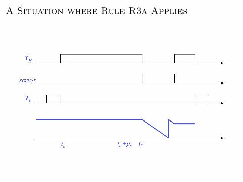
A Situation where Rule R3a Applies

Informal Proof of Correctness
I Correctness: The server never demands more time in anyinterval than corresponding periodic task Ts = (ps, es).
I For now: T has not been idle, and Rule R3b has never applied.
I We show that server “emulates” Task TS = (ps, es).I For this, we view replenishment time as nominal “release
time” of server job.I Each server job only executes at times when a job of TS
would. According to:I Rule C1: Each server job never executes for more than its
budget es
I Rule C2: Budget of idle sporadic server decreases as if serverwas executing.
I On the other hand: C2 means that server holds on to budgetwhen:
I Job in TH is executing. (obviously correct)I Server has not executed since tr. (Actual release time can be
later than nominal release time.)

Informal Proof of Correctness
I Rules R2 and R3(a) make sure that next replenishment timealways set ps time units later than effective release time te.The next effective release time is never earlier than nextreplenishment time.
I R2: Make effective release time as early as possible.
I R3(a): Emulates situation where job in TS takes more time tocomplete than one period.
I R3(b): Applicable only when busy interval of periodic tasksystem ends, and a new one starts. Behavior of tasks in oldbusy period does not affect new busy period.This condition is already accounted for in schedulabilityanalysis of T and Ts.

Enhancements to the Simple SS
I We can improve response times of aperiodic jobs bycombining the Background Server with the Simple SS tocreate a Sporadic/Background Server (SBS).
I Consumption Rules are the same as for the Simple SS exceptwhen the task system T is idle.
I As long as T is idle, the execution budget stays at es.
I Replenishment Rules are the same as for the Simple SS exceptRule R3b.
I The SBS budget is replenished at the beginning of each idleinterval of T. tr is set at the end of the idle interval.

Aperiodic Job Servers for Deadline-Driven
Systems
I The Total Bandwidth Server (TBS) was created by Spuri andButazzo (RTSS 94) to schedule:
I aperiodic task whose arrival time was unknown butI whose worst-case execution time (wcet) was known.I A trivial admission control algorithm used with the TBS can
also schedule sporadic jobs (whose wcet and deadline isknown).
I The constant utilization server was created by Deng, Liu, andSun (Euromicro Workshop 97) to schedule:
I sporadic task whose arrival time was unknown butI whose wcet and deadline was known.I However, they also wanted to schedule aperiodic jobs whose
wcet was unknown.I This server is almost the same as the TBS.

Aperiodic Job Servers for Deadline-Driven
Systems
I Liu’s presentation of the constant utilization server and theTBS is poorly motivated and nearly unintelligible.
I You should read the papers, they make more sense than thematerial in the book.
I We will first cover the TBS and then the constant utilizationserver since it may be easier to understand the value of theconstant utilization server when they are presented in thisorder.

Total Bandwidth Server (TBS)
I One way to reduce the response time of aperiodic jobs whosewcet is known in a deadline-driven system is to
I allocate a fixed (maximum) percentage, US , of the processorto the serve aperiodic jobs, and
I make sure the aperiodic load never exceeds this maximumutilization value.
I When an aperiodic job comes in, assign it a deadline such thatthe demand created by all of the aperiodic jobs in any feasibleinterval never exceeds the maximum utilization allocated toaperiodic jobs.
I This approach is the main idea behind the TBS.
I Note: We use US to denote the server size (as Spuri andButtazzo do) rather than us as Liu does.

TBS in Deadline-Driven Systems
I Let TB be a TBS of size US in a task system T scheduledwith EDF. Thus, the server is allocated US percent of thetotal processor bandwidth.
I The server is ready for execution only when it is backlogged.I In other words: the server is only suspended when it is idle.

TBS in Deadline-Driven Systems
I Consumption Rule: When executing, TB consumes its budgetat the rate of one time unit per unit of execution until thebudget is exhausted.
I Replenishment Rule:
R1 Initially, the execution budget es = 0 and the servers deadlineds = 0.
R2 At time t when aperiodic job Ji with execution time ei arrivesand the server is idle, set ds = max(ds, t) + ei/US andes = ei. If the server is backlogged, do nothing.
R3 When the server completes the currently executing aperiodicjob, Ji,
a If the server is backlogged, update the server deadline andbudget: ds = ds + ei+1/US and es = ei+1.
b If the server is idle, do nothing.

Total Bandwidth Server: Example

TBS Processor Demand
I Observe that the total bandwidth of the server is allocated toone aperiodic job at a time.
I Moreover, if Ji’s execution time is less than its specified wcet,ei, and job Ji+1 arrives before the deadline for job Ji, theTBS effectively performs background execution byreplenishing the servers budget as soon as job Ji is done.
I However, the deadline value ds = max(ds, t) + ei+1/US forjob Ji+1 is is no earlier than ei+1/US time units from thedeadline of job Ji.
I Thus, the demand created by any n jobs in an interval (t1, t2]is at most(
n∑i=1
eieiUs
)=
(n∑
i=1
ei
ei
)Us = nUs ≤ (t2 − t1)Us

Schedulability with a TBS
I Combining this observation with Theorem 6.1, we get thefollowing theorem from Spuri and Buttazzo:
Theorem
A system T of n independent, preemptable, periodic tasks withrelative deadlines equal to their periods is schedulable with a TBSif and only if
UT + US ≤ 1
where UT is the processor utilization of the periodic tasks and US
is the processor utilization of the TBS.

Schedulability with a TBS
I Combining this result with Theorem 6.2, we get the followingtheorem:
Theorem
A system T of n independent, preemptable, periodic tasks withrelative deadlines equal to their periods is schedulable with a TBSif
n∑i=1
ek
min(Dk, pk)+ Us ≤ 1
where US is the processor utilization of the TBS.

Sporadic jobs and the TBS
I Recall that a sporadic job is like an aperiodic job except it hasa hard deadline.
I Assume each sporadic job Ji has a release time ri, wcet ei,and a relative deadline Di: Ji = (ri, ei, Di)
I The TBS assigns deadlines such that the (absolute) deadlinedi assigned any job Ji is
di = max(ri, di−1) + ei/US
where do = 0.
I Thus the TBS can guarantee the deadlines of all acceptedsporadic jobs if it only accepts job Ji+1 if ri+1 + Di+1 ≤ di+1
and rejects it otherwise.

Periodic, Aperiodic, and Sporadic Jobs
I In some systems, we may want to support all three types ofjobs: periodic, aperiodic, and sporadic.
I The TBS can do this by accepting all aperiodic jobs and onlyaccepting a sporadic job if its deadline can be met.
I But there is no value in completing sporadic jobs before theirdeadline, which the TBS will do.
I Thus Deng, Liu, and Sun created the constant utilizationserver (CUS).
I We can schedule sporadic jobs with the CUS and aperiodicjobs with the TBS in the same system.

CUS in Deadline-Driven Systems
I Let TC be a CUS of size US in a task system T scheduledwith EDF.
I As with the TBS, the server is ready for execution only whenit is backlogged. Thus, the server is only suspended when theserver is idle.

CUS in Deadline-Driven Systems
I Consumption Rule: When executing, TC consumes its budgetat the rate of one time unit per unit of execution until thebudget is exhausted.
I Replenishment Rule:
R1 Initially, the execution budget es = 0 and the servers deadlineds = 0.
R2 At time t when aperiodic job Ji with execution time ei arrivesand the server is idle,
a If t < ds, do nothing;b If t ≥ ds, ds = t + ei/US and es = ei.
R3 At the deadline ds of the server,
a If the server is backlogged, update the server deadline andbudget: ds = ds + ei+1/US and es = ei+1
b If the server is idle, do nothing.

Total Bandwidth Server: Example

Aperiodic Jobs with Unknown Execution Times
I Assumption for constant utilization server: execution times ofaperiodic jobs are known upon arrival.
I Possible solution: Assign fixed bandwidth to server:I fixed budget es
I fixed period es/us
I Upon job completion of job with execution time e < es,reduce current deadline of server by (es − e)/us beforereplenishing again.
I For execution time e > es, use more than one server period.

Comments on the CUS
I Deadlines and replenish amounts are the same in both servers.
I The main difference between the CUS and the TBS is thatthe CUS never replenishes the servers budget early.
I Thus, the TBS actually yields better average response timesfor aperiodic jobs (and it was created before the CUS ...)
I Moreover, it would appear that the TBS may be able toaccept more sporadic jobs than the CUS.
I The value of the CUS is not clear, and Liu does a terrible jobarguing for it!

TBS and CUS Summary
I Both servers can be modified to support the case when thewcet of aperiodic jobs is unkown:
I fix the execution budget at some value es and assume theserver has a period of es/US .
I Both servers can be modified to reclaim unused resourceswhen the actual execution time e is less than the wcet es thatwe assumed:
I reduce the current deadline of the server by (es − e)/US unitsbefore replenishing the budget.
I We can have multiple TBS/CUS servers as long as the totalprocessor utilization/density is not greater than 1.

Non-Preemptable Portions
I Non-preemptable portions either reduce schedulable utilizationor introduce tardiness.
I Definitions:I bmax(np) is maximum execution time of non-preemptable
portions of periodic tasks and jobs executed by servers.I effective execution time of job executed by server: ratio of job
execution time and server size.I Dmin is minimum of all relative deadlines of periodic tasks and
effective execution times of jobs executed by all servers.
Corollary
When a system of periodic tasks is scheduled with one or moretotal bandwidth and constant utilization server on the EDF basis,every periodic task and every server meets its deadline if the sumof the total density of the periodic tasks and the total size of allservers is no greater than 1− bmax(np)/Dmin.

Fairness and Starvation
I Total Bandwidth Server is not fair
I Example: TB1 and TB2 each of size 0.5I If both servers never idle, service is approximately equally
shared among servers.I With idling servers, this is not always the case.
I Processor time is allocated fairly during (0, t), but not during(t, 2t). And t can be arbitrary large.

Fairness and Starvation
I wi(t1, t2) = total total attained processor time for Server iduring time interval (t1, t2).
I wi(t1, t2)/ui = normalized service.
Definition
Scheduler is fair during interval (t1, t2) if normalized serviceattained by all servers does not differ by more than a fairnessthreshold FR.
I Ideally, FR is zero:
wi(t1, t2)wj(t1, t2)
=ui
uj⇐⇒ wi(t1, t2) = ui(t2 − t1)

Eliminating Starvation
I Problem with Total Bandwidth server: When processing timeavailable, allows to indefinitely put deadlines into the future.
I A simple solution to this is to use only constant utilizationservers.
I Constant Utilization server keeps deadlines “close”:
d− t ≤ ei,max/ui
where ei,max is the maximum execution time of jobs served byServer i.
I Hence the the length of starvation suffered by any server isbounded by maxi(ei,max/ui).
I We can improve the CUS to make better use of backgroundtime (fairly).

Starvation-free CUS/Background Server
I Replenishment rules for starvation-free Constant Utilization/Background server:
R1 - R3 Same as Constant Utilization server.R4 Whenever busy interval ends, replenish budget of all
backlogged servers.
I Note: Background time is not distributed to backloggedservers according to their size =⇒ starvation is eliminated,but not unfairness.

Proportional Share Scheduling
I Proposed by Stoica et. al. (1996)I Processes are allocated a share of a shared resource:
I a relative percentage of the resources total capacity.
I Processes make progress at a uniform rate according to theirshare.
I OS Example time sharing tasks allocated an equal share(1/n) of the processors capacity. Round robin scheduling,fixed size quantum

Formal Allocation Model
I Processes are allocated a share of the processors capacity.
I Process i is assigned a weight wi (a rational number).
I Process is share of the CPU at time t is
fi(t) =wi∑j wj
I Note: in the denominator of fi(t) we are summing over onlythe active processes in the system; all tasks in the case of areal-time system.

Formal Allocation Model
I If processes weights remain constant in [t1, t2] then process ireceives units of execution time in [t1, t2] for a fluid-allocationsystem (quantum can be arbitrary small).
Si(t1, t2) =∫ t2
t1
fi(t)dt =wi∑j wj
(t2 − t1)
I Some comments on Si(t1, t2):I The definition of the integral Si() is always correct.I The assumption that weights remain constant over the interval
lets us reduce the integral to a linear equation.I Otherwise, we can generate a piecewise linear equation.

Formal Allocation Model
I Ignoring weights for a moment, we note that there is a simpleproof that utilization ≤ 1 is a sufficient condition forschedulability when each task Ti is allocated a fraction ofeach time unit equal to its utilization ei/pi.
I Thus, we can schedule periodic tasks with a round robinscheduling algorithm if we assume an infinitesimally smallquantum and allocate each task a share equal to theirprocessor utilization ei/pi within each time unit.

Real-Time Scheduling Example
I Now consider the same task set with RR scheduling and avariable-sized quantum. Assume a round length of 2.
I Thus, the share of task Ti in each round (of length 2) is2(ei/pi).
I Here down arrows represent releases (or a job entering thesystem). and up arrows represent deadlines (or a job leavingthe system).

Real-Time Scheduling Example
I Round robin scheduling with an integer, variable-sizedquantum and a round length of 4:
I Notice that, in this and the last two examples, the processor isidle at least 25% of each round, even when there are readytasks.
I In these examples, the scheduling algorithm isnon-workconserving.
I However, each process always receives its share in each round.

Real-Time Scheduling Example
I A more realistic scheduling scenario would be round robinscheduling with a fixed size quantum.
I Consider a fixed sized quantum of 1 and a round length of 2:
I Notice that T1 is not scheduled in [4, 8) because it has alreadycompleted execution.
I It received more that its share in [0, 4) and less in [4, 8)

Scheduling Sporadic Tasks in Deadline-driven
Systems Systems
I Total density of periodic tasks is ∆.
I As long as total density of sporadic jobs does not exceed1−∆ , all deadlines can be maintained by EDF.
I The acceptance test on the first sporadic job S(t, d, e) issimple. The scheduler accepts S if its density e/(d− t) is nogreater than 1−∆.
I If the schedule accepts S, we will have two distinct intervalswith respect to task densities:
I I1 = [t, d) with density ∆s,1 = ∆ + e/(d− t) andI I2 = [d,∞) with density ∆s,2 = ∆

Scheduling Sporadic Tasks in Deadline-driven
Systems Systems
I In the general case, at a time t there can be ns sporadic jobsalready accepted in the system.
I For the purpose of scheduling, the scheduler maintains anondecreasing list of (absolute) deadlines of accepted jobs.
I These deadlines partitions the time interval [t,∞) into ns + 1disjoint intervals. I1, . . . , Ins+1.
I The scheduler also keeps up-to-date the total density ∆s,k ofthe sporadic jobs that are active during each of these intervals.
I Let Il be the time interval containing the deadline d of thenew sporadic job S(t, d, e). The scheduler will accept the jobS if
e
d− t+ ∆s,k ≤ 1−∆

Scheduling Sporadic Tasks in Deadline-driven
Systems Systems
I If the scheduler accepts S it divides the interval Il into twointervals at separated at d.
I The complexity of this acceptance test is O(Ns) where Ns isthe maximum number sporadic jobs that can be scheduled inthe same time.

Resources and Resource Access Control
I Until now, we have assumed that tasks are independent.
I We now remove this restriction.
I We consider how to adapt the analysis discussed previouslywhen tasks access shared resources.

Mars Pathfinder Incident
I Landing on July 4, 1997
I experiences softwareglitches.
I Pathfinder experiencesrepeated RESETs afterstarting gathering ofmeteorological data.
I RESETs generated bywatchdog process.
I Timing overruns causedby priority inversion.
See: research.microsoft.com/ mbj/Mars Pathfinder/Mars Pathfinder.html

Priority Inversion on Mars Pathfinder

Shared Resources
I We continue to consider single-processor systems.
I We add to the model a set of ρ serially reusable resourcesR1, R2, . . . , Rρ, where there are vi units of resource Ri.
I Examples of resources:I Binary semaphore, for which there is one unit.I Counting semaphore, for which there may be many units.I Reader/writer locks.I Printer.I Remote server.

Locks
I A job that wants n units of resource R executes a lockrequest, denoted L(R,n).
I It unlocks the resource by executing a corresponding unlockrequest, denoted U(R,n).
I A matching lock/unlock pair is a critical section.
I A critical section corresponding to n requested units ofresource R, with an execution cost of e, will be denoted[R,n; e]. If n = 1, then this is simplified to [R; e].

Locks
I Locks can be nested.I We will use notation like this:
I [R1; 14[R4, 3; 9[R5, 4; 3]]]
I In our analysis, we will be mostly interested in outermostcritical sections.
I Note: For simplicity, we only have one kind of lock request.I So, for example, we cant actually distinguish between reader
locks and writer locks.

Conflicts
I Two jobs have a resource conflict if some of the resourcesthey require are the same.
I Note that if we had reader/writer locks, then notion of a“conflict” would be a little more complicated.
I Two jobs contend for a resource when one job requests aresource that the other job already has.
I The scheduler will always deny a lock request if there are notenough free units of the resource to satisfy the request.

Example

Timing Anomalies
I When tasks share resources, there may be timing anomalies.
I Example: Let us reduce J3’s critical section execution from 4time units to 2.5. Then J1 misses its deadline!

Priority Inversions
I When tasks share resources, there may be priority inversions.

Deadlocks
I When tasks share resources, deadlocks may be a problem.
I Example: J1 accesses green, then red (nested). J3 accessesred, then green (nested).

Wait-for Graphs
I We will specify blocking relationships using a wait-for graph.

Specifying Resource Requirements
I Resource requirements will be specified like this:

Resource Access Control Protocols
I We now consider several protocols for allocating resourcesthat control priority inversions and/or deadlocks.
I From now on, the term critical section is taken to meanoutermost critical section unless specified otherwise.

Nonpreemptive Critical Section Protocol
I The simplest protocol: just execute each critical sectionnonpreemptively.
I If tasks are indexed by priority (or relative deadline in the caseof EDF), then task Ti has a blocking term equal to
maxi+1≤k≤n
ck,
where ck is the execution cost of the longest critical section ofTk.
I Disadvantage: Ti’s blocking term may depend on tasks that itdoesn’t even have conflicts with.

Nonpreemptive Critical Section Protocol
I Analysis identical to analysis with non-preemptable portions.
I Define: β = maximum duration of all critical sections
I Task Ti is schedulable if
i∑k=1
ek
pk+
β
pi≤ UX(i)

The Priority Inheritance Protocol
I Observation: In a system with lock-based resources, priorityinversion cannot be eliminated.
I Thus, our only choice is to limit their duration. Consideragain this example:

The Priority Inheritance Protocol
I The problem here is not the low-priority job J3 – its themedium priority job J2!
I We must find a way to prevent a medium-priority job like thisfrom lengthening the duration of a priority inversion.

The Priority Inheritance Protocol
I Priority Inheritance Protocol: When a low-priority job blocks ahigh-priority job, it inherits the high-priority jobs priority.
I This prevents an untimely preemption by a medium-priorityjob.

The Priority Inheritance Protocol
I Each job Jk has an assigned priority (e.g., RM priority) and acurrent priority πk(t).
1. Scheduling Rule: Ready jobs are scheduled on the processorpreemptively in a priority-driven manner according to theircurrent priorities. At its release time t, the current priority ofevery job is equal to its assigned priority. The job remains atthis priority except under the condition stated in rule 3.
2. Allocation Rule: When a job J requests a resource R at t,
2.1 if R is free, R is allocated to J until J releases it, and2.2 if R is not free, the request is denied and J is blocked.
3. Priority-Inheritance Rule: When the requesting job J becomesblocked, the job Jl that blocks J inherits the current priorityof J . The job Jl executes at its inherited priority until itreleases R (or until it inherits an even higher priority); thepriority of Jl returns to its priority πl(t′) at the time t′ when itacquires the resource R.

Example

A more Complicated Example
I Problem: If T5 tries to lock(B) while it has priority π1, wehave a deadlock!

Properties of Priority Inheritance Protocol
I It does not prevent deadlock.
I Task can be blocked directly by a task with a lower priority atmost once, for the duration of the (outmost) critical section.
I Consider a task whose priority is higher than n other tasks:
I Each of the lower-priority tasks can directly block the task atmost once.

The Priority-Ceiling Protocol
I Two key assumptions:I The assigned priorities of all jobs are fixed (as before).I The resources required by all jobs are known a priori before the
execution of any job begins.
I Definition: The priority ceiling of any resource R is the highestpriority of all the jobs that require R, and is denoted Π(R) orΠR.
I Any task holding R may have priority Π(R) at some point;either its own priority is Π(R), or it inherits Π(R).
I Definition: The current priority ceiling Π(t) (at time t) of thesystem is equal to the highest priority ceiling of the resourcescurrently in use, or Ω if no resources are currently in use.
I Ω is a priority lower than any real priority).

The Priority-Ceiling Protocol: Motivation
I Suppose there are resource A and B.
I Both A and B are available. T1 requests A.
I T2 requests B after A is allocated.
I If π2 > Π(A) : T1 can never preempt T2 =⇒ B should beallocated to T2.
I If π2 ≤ Π(A) : T1 can preempt T2 (and also request B) atsome later time. B should not be allocated to T2, to avoiddeadlock.

The Priority-Ceiling Protocol: Definition
I Scheduling Rule:
1. At its release time t, the current priority π(t) of every job Jequals its assigned priority. The job remains at this priorityexcept under the conditions of rule 3.
2. Every ready job J is scheduled preemptively and in apriority-driven manner at its current priority π(t).
I Allocation Rule: Whenever a job J requests a resource R attime t, one of the following two conditions occurs:
a R is held by another job. J ’s request fails and J becomesblocked.
b R is free.
i If J ’s priority π(t) is higher than the current priority ceilingΠ(t), R is allocated to J .
ii If J ’s priority π(t) is not higher than the ceiling Π(t), R isallocated to J only if J is the job holding the resource(s)whose priority ceiling equals Π(t); otherwise, J ’s request isdenied and J becomes blocked.

The Priority-Ceiling Protocol: Definition
I Priority-Inheritance Rule: When J becomes blocked, the jobJl that blocks J inherits the current priority π(t) of J . Jl
executes at its inherited priority until it releases every resourcewhose priority ceiling is ≥ π(t) (or until it inherits an evenhigher priority); at that time, the priority of Jl returns to itspriority π(t′) at the time t′ when it was granted the resources.

Example

Another Example

Schedulability Analysis
I Blocking: A higher-priority task waits for a lower-priority task.
I A task TH can be blocked by a lower-priority task TL in threeways:

Schedulability Analysis: Preliminary
Observations
I Consider: Task T with priority π and at release time t.
Preliminary Observation 1
T cannot be blocked if at time t, when every resource allocatedhas a priority ceiling less than π, i.e., π > Π(t).
I No task with priority lower than π holds any resource withpriority ceiling ≥ π.
I T will not require any of the resources allocated at time twith priority ceilings < π, and will not be directly blockedwaiting for them.
I No lower-priority task can inherit a priority higher than πthrough resources allocated at time t.
I Requests for resources by T will not be denied because ofresource allocations made before t.

Schedulability Analysis: Preliminary
Observations
Preliminary Observation 2
Suppose that
I There is a task TL holding a resource X
I T (with priority π) preempts TL, and then
I T is allocated a resource Y .
Until T completes, TL cannot inherit a priority higher or equal to π.
Reason: (πL = priority of TL when it is preempted.)
I πL < π
I T is allocated a resource =⇒ π is higher than all the priorityceilings of resources held by all lower-priority tasks when Tpreempts TL.
I T cannot be blocked by TL, from Preliminary Observation 1=⇒ πL cannot be raised to π or higher through inheritance.

Schedulability Analysis with Resources
Access
I Schedulability loss due to blocking:
I Reminder: Critical sections are properly nested =⇒ Durationof a critical section equals the outmost critical section.
Observation 1
A low-priority task TL can block a higher-priority task TH at mostonce.
Reason: When TL is not in critical section
I πL < πH
I TL cannot inherit a higher priority

Schedulability Analysis with Resources
Access
Observation 2
A task T can be blocked for at most the duration of one criticalsection, no matter how many tasks share resources with T .
Reason:
I It is not possible for T to be blocked for durations of 2 criticalsections of one task.
I It is not possible for T to be blocked by T1 and T2 withpriorities π1 < π , π2 < π.

Two Theorems
Theorem (8.1)
When the resource accesses of a system of preemptive,priority-driven jobs on one processor are controlled by the PCP,deadlock can never occur.
Theorem (8.2)
When the resource accesses of a system of preemptive,priority-driven jobs on one processor are controlled by the PCP, ajob can be blocked for at most the duration of one critical section.

Deadlock Avoidance
I With the PIP, deadlock could occur if nested critical sectionsare invoked in an inconsistent order. Heres an example welooked at earlier.
I Example: J1 accesses green, then red (nested). J3 accessesred, then green (nested).
I The PCP would prevent J1 from locking green. Why?

Deadlock Avoidance
I Suppose J1 blocks when accessing the green critical sectionand later blocks when accessing the red critical section.

Deadlock Avoidance
I For J1 to block on green, some lower-priority job must haveheld the lock on green when J1 began to execute.

Deadlock Avoidance
I For J1 to later block on red, some lower-priority job musthave held the lock on red when J1 began executing.

Deadlock Avoidance
I Whichever way J2 and J3 are prioritized (here, J2 has priorityover J3), we have a contradiction. Why?

Blocking Terms
I When computing blocking terms, it is important to carefullyconsider all three kinds of blocking (direct, inheritance,ceiling).
I See the book for an example where this is done systematically(Figure 8-15).
I With the PCP, we have to pay for extra two context switchesper blocking term.
I Such context switching costs can really add up in a largesystem.
I This is the motivation for the Stack Resource Policy (SRP),described next.

Stack Sharing
I Sharing of the stack among tasks eliminates stack spacefragmentation and so allows for memory savings:
I However:I Once job is preempted, it can only resume when it returns to
be on top of stack.I Otherwise, it may cause a deadlock.I Stack becomes a resource that allows for one-way preemption.

Stack Sharing
I If tasks share a runtime stack, we clearly cannot allow aschedule like the following. (Why?)
I We must delay the execution of each job until we are sure allthe resources it needs are available.

Stack-Sharing Priority-Ceiling Protocol
I Define: Π(t) highest priority ceiling of all resources currentlyallocated. If no resource allocated, Π(t) = Ω.
I Protocol:
1. Update Priority Ceiling: Whenever all resources are free,
Π(t) = Ω. The value of Π(t) is updated whenever resource isallocated or freed.
2. Scheduling Rule: After a job is released, it is blocked from
starting execution until its assigned priority is higher then Π(t).At all times, jobs that are not blocked are scheduled on theprocessor in a priority-driven, preemptive fashion according totheir assigned priorities.
3. Allocation Rule: Whenever a job requests a resource, it isallocated the resource.

Stack Sharing

Stack-Sharing Priority-Ceiling Protocol
I The Stack-Based Priority-Ceiling Protocol is deadlock-free:I When a job begins to execute, all the resources it will ever
need are free.I Otherwise, Π(t) would be higher or equal to the priority of the
job.I Whenever a job is preempted, all the resources needed by the
preempting job are free.I The preempting job can complete, and the preempted job can
resume.
I Worst-case blocking time of Stack-Based Protocol is the sameas for Basic Priority Ceiling Protocol.
I Stack-Based Protocol has smaller context-switch overheadthan Priority Ceiling Protocol.
I Once execution starts, job cannot be blocked.

Ceiling-Priority Protocol
I Stack-Based Protocol does not allow for self-suspension.
I Re-formulation for multiple stacks (no stack-sharing)straightforward:
I Ceiling-Priority Protocol:I Scheduling Rules:
1. Every job executes at its assigned priority when it does nothold resources.
2. Jobs of the same priority are scheduled on FIFO basis.3. Priority of jobs holding resources is the highest of the priority
ceilings of all resources held by the job.
I Allocation Rule: Whenever a job requests a resource, it isallocated the resource.

Multiprocessor/Distributed Systems
I Many real-time systems contain more than a single processor.I A multiprocessor system is tightly coupled and usually has
shared-memory.I There may be one scheduler for all processors, but this type of
scheduling is usually NP-Hard.I Or, there may be a scheduler for each processor, which is the
model we will assume.
I A distributed system is loosely coupled; it is costly to keepglobal status. There is usually one scheduler for eachprocessor.

Multiprocessor/Distributed Systems
I We assume each processor has its own scheduler and localresources.
I Local resources may be shared globally, but access to them iscontrolled locally.
I All of the same problems with scheduling and shared resourcesthat we discussed on single processors exist on multiprocessorand distributed systems, but the problems are even harder tosolve!

Multiprocessors and Resource Access
Control
I We first consider how to adapt the analysis discussedpreviously when tasks access globally shared resources frommultiple processors in a tightly-coupled systems.
I Later, in our discussion of distributed systems, we willconsider tasks that have precedence constraints, and the taskmay execute in a distributed system.

A Review of Shared Resources
I In multiprocessor systems we will assume a resource is“hosted” on one processor, but accessible from each processor.
I We add to the model a set of r serially reusable resourcesR1, R2, . . . , Rr, where there are vi units of resource Ri.
I Examples of resources:I Binary semaphore, for which there is one unit.I Counting semaphore, for which there may be many units.I Reader/writer locks.I Printer.I Remote server.

A Review of Conflicts
I Two jobs have a resource conflict if some of the resourcesthey require are the same.
I Note that if we had reader/writer locks, then notion of a“conflict” would be a little more complicated.
I Two jobs contend for a resource when one job requests aresource that the other job already has.
I The scheduler will always deny a lock request if there are notenough free units of the resource to satisfy the request.

Multiprocessor Priority-Ceiling Protocol
I The Multiprocessor Priority-Ceiling Protocol (MPCP) wascreated by Sha, Rajkumar, and Lehoczky (1988).
I It assumes that tasks and resources are statically bound toprocessors.
I The host processor for a resource is called the synchronizationprocessor for that resource.
I The fixed priority scheduler for each synchronization processorknows the priorities and resources requirements of all tasksrequiring access to its globally shared resources.

Multiprocessor Priority-Ceiling Protocol
I Access to globally shared resources is controlled locally on thesynchronization processor according to the Priority-CeilingProtocol (PCP) we covered earlier, with the followingexceptions:
I Access to a globally shared resource is modeled as the taskexecuting a global critical section on the synchronizationprocessor for the resource.
I All global critical sections are executed at higher priorities thanlocal tasks on the synchronization processor.

Simple MPCP Example

Distributed Real-Time Systems
I In many distributed systems the workload can be modeled asa set of tasks in which some tasks consist of subtasks thatexecute on different processors:
I The subtasks are released according to precedence constraints.That is, T2,2 cannot be released until task T2,1 completes.

End-To-End Scheduling
I The scheduling problem now becomes one of guaranteeingend-to-end response times in a distributed system withprecedence constraints.
I We assume that each subtask (or task if it has no subtasks)accesses only local resources.
I Thus, we simplify the end-to-end scheduling problem bydecomposing it to a set of similar scheduling problems that wehave already discussed: single processor scheduling.
I We need only worry about scheduling tasks (with access tolocal resources) on a single processor and obeying precedenceconstraints.

End-To-End Scheduling
I We can use any scheduling algorithm we want as long as wecan bound response times.
I We can even use a different algorithm on each processor.
I All we need is a synchronization protocol that ensuresprecedence constraints are met.

Synchronization Protocols
I Work-conserving:I Direct Synchronization (DS) Protocol
I Liu calls this the Greedy Synchronization Protocol.I Simple and low overhead, but may results in large release-time
and/or finish-time jitter.
I Release-Guard (RG) Protocol (Sun) – we cover this lastI Combines MPM with DS.
I Non-work-conserving:I Overcomes release/finish-time jitter by shaping the releasetime
patterns of subtasks.I Non-work-conserving protocols are usually time-driven and
require synchronized clocks (which creates new problems).I Phase-Modification (PM) Protocol (Bettati)I Modified Phase-Modification (MPM) Protocol

Direct Synchronization (DS) Protocol
I As soon as a subtask finishes executing, it sends asynchronization signal (e.g., message) to the downstream(sibling) subtask in the task chain.
I For example:
I Each subtask is released as soon as its predecessor completes,e.g., as soon as a message arrives.

RM Execution Example with DS

EDF Execution Example with DS

Advantages of DS Protocol
I It is the most commonly used protocol, especially innon-real-time systems.
I The DS protocol is simple and can be implemented in manyways.
I Global clock synchronization is not needed.
I Yields the shortest average end-to-end response time of alltasks when compared with the other synchronizationprotocols.

Disadvantages of DS Protocol
I Some synchronized tasks may have extremely large end-to-endresponse times when scheduled with a fixed priority schedulerat each processor (even though this protocol yields the lowestaverage response time).
I The DS protocol often results in bursty release times ofdownstream subtasks.
I This can affect the schedulability of end-to-end tasks in fixedpriority driven systems.
I The Rate-Based Execution Model was created to address thisproblem.
I It is difficult to assign priorities for subtasks on differentprocessors in a priority-driven system.

Phase-Modification (PM) Protocol
I The PM protocol maintains a minimum temporal distancebetween the release times of jobs in sibling subtasks of a taskchain.
I The earliest release time of each subtask is some fixed amountof time after the release of immediate predecessor subtask inthe task chain.
I Let Wi,k be the maximum response time of every subtask Ti,k
on processor Vi,k. The jth job Ji,k+1;j of subtask Ti,k+1 isreleased on processor Vi,k+1 at time
φi + (j − 1)pi +k∑
l=1
Wi,l
Where the release time of the jth job in Ti,1 is φi + (j − 1)pi.

RM Execution Example with PM

Advantages of PM Protocol
I Very simple concept.I Easy to implement when
I clocks are synchronized,I the first subtask of every task chain is released periodically, andI Wi,k of each subtask is available to the downstream scheduler.
I Each subtask is always released periodically if the first subtaskis a periodic task.
I End-to-End response time is simply the sum
Wi =n(i)∑l=1
Wi,l
where n(i) is the number of subtasks in task Ti.

Disadvantages of PM Protocol
I Requires global clock synchronization and global informationon upper bounds to response times.
I If there is any release-time jitter in the first subtasks, as isoften the case, then the PM protocol may violate aprecedence constraint.
I It is difficult to get tight (and precise) bounds on themaximum response time Wi,k of each subtask.

Modified Phase-Modification (MPM)
Protocol
I The MPM protocol combines the synchronization message ofDS with phase modification of PM.
I The only difference between PM and MPM is that eachsuccessor job Ji,k+1;j is released at the later of Wi,k timeunits after the release of its predecessor job Ji,k;j and theactual completion time of Ji,k;j .
I A simple implementation is for the scheduler of Vi,k to send asynchronization signal to the scheduler of Vi, k + 1 when thedownstream job Ji,k+1;j should be released.
I This way we do not need synchronized clocks, andI Release-time jitter of the first sub-task is propagated
throughout the task chain to maintain precedence constraints.

RM Execution Example with MPM

Advantages of MPM Protocol
I Does not require a global clock!I Easy to implement even when
I clocks are not synchronized, orI the first subtask of every task chain is not released periodically.
I Wi,k of each subtask is not needed by the downstreamscheduler.
I Correct even with job overrun or release-time jitter (sporadicrelease times) for the first subtask in the task chain.

Disadvantages of MPM Protocol
I The successor subtask Ti,k+1 may no longer behave like aperiodic task when an upstream job overruns its wcet.
I Thus, the scheduling analysis on two processors may beincorrect!
I The non-work-conserving nature of the protocol increasesaverage response times unnecessarily when the downstreamprocessor is idle.
I This was also true with PM.

Release-Guard (RG) Protocol
I Let ri,k;j be the release time of job Ji,k;j on processor Vi,k;j .
I The scheduler of Vi,k sends a synchronization signal to thescheduler of Vi,k+1 as soon as job Ji,k;j completes.
I The scheduler of Vi,k+1 releases the first job Ji,k+1;1 ofsubtask Ti,k when it receives the first synchronization signalfor the subtask.
I For j > 1, if the processor is busy in the interval[ri,k+1;j−1, ri,k+1;j−1 + pi],R1 job Ji,k+1;j is released at the later of when thesynchronization signal is received from the predecessor jobJi,k;j and ri,k+1;j−1 + pi.
I Otherwise,R2 for j > 1, job Ji,k+1;j is released at the later of when thesynchronization signal is received from the predecessor jobJi,k;j and when the processor becomes idle.

Intuition Behind (RG) Protocol
I Intuitively, the RG protocol makes sure that the inter-releasetime of any two consecutive jobs of the same subtask arenever less than the period of the subtask.
I But it will release jobs early when doing so will not affect theschedulability of lower-priority subtasks.

RM Execution Example with RG

Advantages of RG Protocol
I Work-conserving:I Takes advantage of idle time to reduce end-to-end response
times.
I Does not require a global clock!
I Wi,k of each subtask is not needed by the downstreamscheduler.
I Correct even with job overrun or release-time jitter (sporadicrelease times) for the first subtask in the task chain.
I Liu gives no disadvantages!I Can you think of any?

Relative Performance of the Four Protocols
I The DS has low overhead/complexity and the shortestaverage end-to-end response (EER) times.
I However, it can result in very long worst-case EER times.
I The RG protocol yields better average EER than PM orMPM.
I However, output jitter is much worse than that produced byPM or MPM.
I Liu indicates that if output jitter is a concern, you can use RGand simply ignore rule R2.
I Liu contends that RG is almost always better than DS inactual systems because of the shorter worst-case EER timesRG yields.