EE101

EE101 Introduction to Electrical

Engineering

Statistical Signal Processing

Instructor: Bilge Karaçalı, PhD

EE101

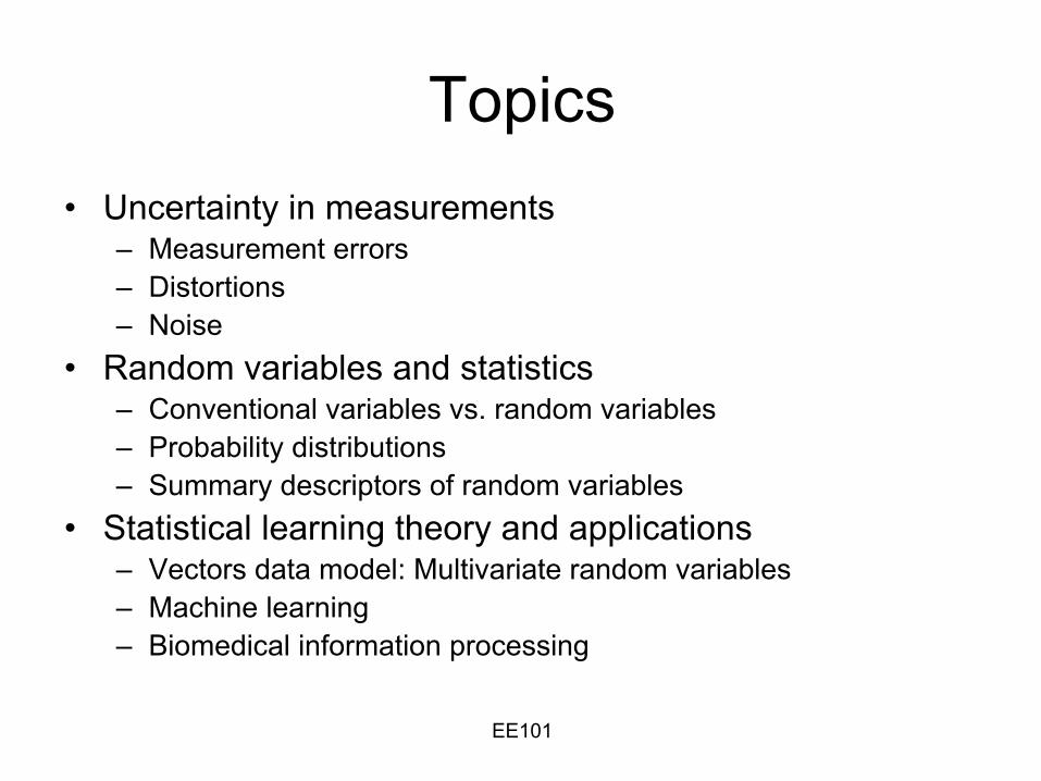
Topics•

Uncertainty in measurements–

Measurement errors–

Distortions –

Noise •

Random variables and statistics–

Conventional variables vs. random variables–

Probability distributions–

Summary descriptors of random variables•

Statistical learning theory and applications–

Vectors data model: Multivariate random variables–

Machine learning–

Biomedical information processing

EE101

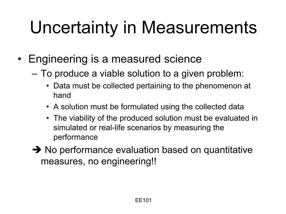
Uncertainty in Measurements

•

Engineering is a measured science–

To produce a viable solution to a given problem:

•

Data must be collected pertaining to the phenomenon at hand

•

A solution must be formulated using the collected data•

The viability of the produced solution must be evaluated in simulated or real-life scenarios by measuring the performance

No performance evaluation based on quantitative measures, no engineering!!

EE101

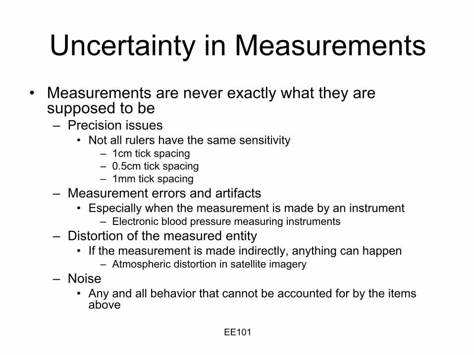
Uncertainty in Measurements•

Measurements are never exactly what they are supposed to be–

Precision issues•

Not all rulers have the same sensitivity–

1cm tick spacing–

0.5cm tick spacing–

1mm tick spacing–

Measurement errors and artifacts •

Especially when the measurement is made by an instrument–

Electronic blood pressure measuring instruments–

Distortion of the measured entity•

If the measurement is made indirectly, anything can happen–

Atmospheric distortion in satellite imagery–

Noise•

Any and all behavior that cannot be accounted for by the items above

EE101

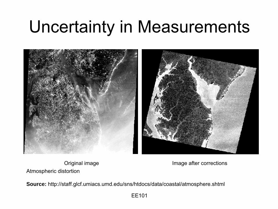
Uncertainty in Measurements

Atmospheric distortion

Source: http://staff.glcf.umiacs.umd.edu/sns/htdocs/data/coastal/atmosphere.shtml

Original image Image after corrections

EE101

Uncertainty in Measurements

Above: Image with a long exposure timeSource: http://digital-photography-school.com/long-

exposure-photography

Right: Under and over exposure Source: http://all-about-camera.blogspot.com/

EE101

Random Variables•

Quantifiable entities that may exhibit different values depending on factors beyond our control are represented by:

random variables–

The outcome of a “measurement”

activity is represented by a random variable

•

Each time you repeat the measurement, the readout may change beyond your control

–

Control underlies the difference between a conventional variable

and a random variable

•

But overall, the readouts tend to accumulate near some values while some other values rarely ever show up

•

Distribution of values observed by a random variable are characterized by its

probability distribution

EE101

Random Variables•

Random variables can be–

discrete or continuous–

univariate

or multivariate•

Probability distribution functions determine how likely it is to

observe a given outcome–

Let the random variable D denote the outcome of a fair die throwing experiment

Pr{D = 1} = FD(1) = 1/6Pr{D = 2} = FD (2) = 1/6Pr{D = 3} = FD (3) = 1/6Pr{D = 4} = FD (4) = 1/6Pr{D = 5} = FD (5) = 1/6Pr{D = 6} = FD (6) = 1/6

–

This means, if you throw the die many times, the total number of

times you get a 1 will be about the same as another number

EE101

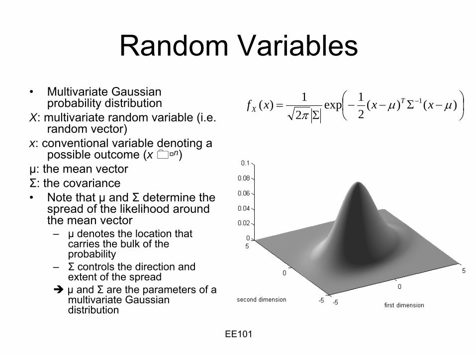
Random Variables•

Multivariate Gaussian probability distribution

X: multivariate random variable (i.e. random vector)

x: conventional variable denoting a possible outcome (x n)

μ: the mean vectorΣ: the covariance•

Note that μ

and Σ

determine the spread of the likelihood around the mean vector

–

μ

denotes the location that carries the bulk of the probability

–

Σ

controls the direction and extent of the spreadμ and Σ are the parameters of a multivariate Gaussian distribution

⎟⎠⎞

⎜⎝⎛ −Σ−−

Σ= − )()(

21exp

21)( 1 μμπ

xxxf TX

EE101

Statistical Learning Theory

•

Objective: to construct mathematical rules that make accurate decisions for recognition problems based on empirical observations–

Decision making via mathematical rules

–

Recognition problems–

Empirical observationsTo decide upon a random variable/vector

using its statistical characterization

EE101

Statistical Learning Theory•

Example:–

Goal: to be able to decide whether a cell is benign or cancerous

based on a set of quantitative features collected into a feature vector

•

Radius•

Texture•

Perimeter•

Area•

…–

Approach: •

Identify a large collection of cells–

Some of the cells to be benign, others cancerous•

Determine which ones are benign and which ones are cancerous using help from an expert pathologist

•

Measure the features of every cell•

Construct a mathematical function of that returns –

Positive values when the associated cell is malignant–

Negative values when the cell is benignWisconsin Breast Cancer Dataset

EE101

Statistical Learning Theory•

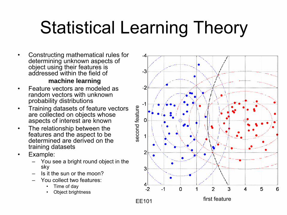
Constructing mathematical rules for determining unknown aspects of object using their features is addressed within the field of

machine learning•

Feature vectors are modeled as random vectors with unknown probability distributions

•

Training datasets of feature vectors are collected on objects whose aspects of interest are known

•

The relationship between the features and the aspect to be determined are derived on the training datasets

•

Example:–

You see a bright round object in the sky

–

Is it the sun or the moon?–

You collect two features:•

Time of day•

Object brightness

seco

nd fe

atur

e

first feature

EE101

Example: Nearest Neighbor Classification

•

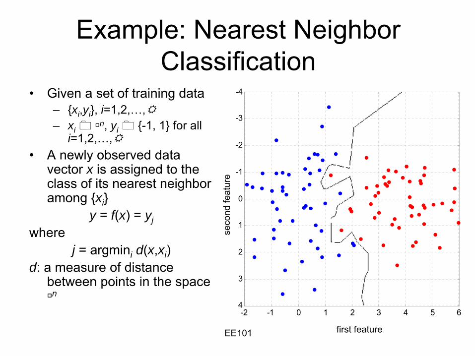
Given a set of training data –

{xi ,yi }, i=1,2,…,–

xin, yi {-1, 1} for all

i=1,2,…,•

A newly observed data vector x is assigned to the class of its nearest neighbor among {xi }

y = f(x) = yjwhere

j = argmini d(x,xi )d: a measure of distance

between points in the space n

-2 -1 0 1 2 3 4 5 6

-4

-3

-2

-1

0

1

2

3

4

seco

nd fe

atur

e

first feature

EE101

Biomedical Information Processing•

Technological innovations in life sciences research–

Development of biosensor technologies•

Medical imaging systems•

Immunohistochemical staining•

Electrophysiological monitoring•

…–

Introduction of high-throughput techniques•

DNA microarrays•

Flow cytometry•

…•

Increasing difficulty in analyzing rapidly accumulating biological data using conventional manual techniques–

Time–

Quantitation–

Standardization–

DimensionalityProcessing of biomedical information using machine learning algorithms

EE101

Biomedical Information Processing

•

Involves biology and medicine•

Operates on information represented by quantitative data

•

Makes inferences on the problems of interest using computational algorithms

EE101

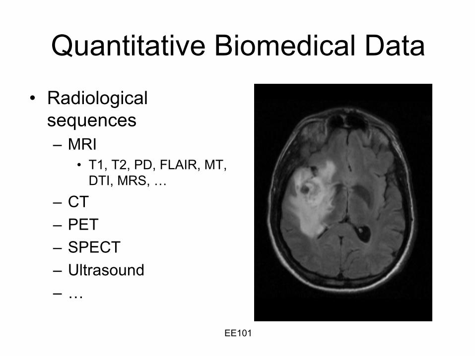
Quantitative Biomedical Data

•

Radiological sequences–

MRI

•

T1, T2, PD, FLAIR, MT, DTI, MRS, …

–

CT–

PET

–

SPECT–

Ultrasound

–

…

EE101

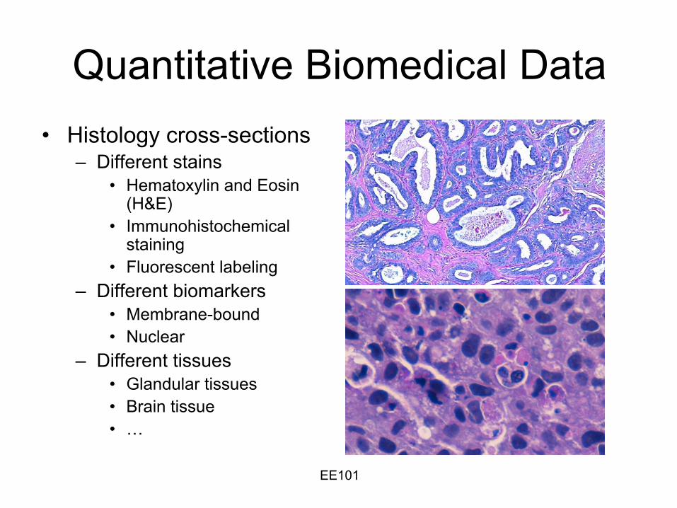
Quantitative Biomedical Data•

Histology cross-sections–

Different stains•

Hematoxylin

and Eosin (H&E)

•

Immunohistochemical staining

•

Fluorescent labeling–

Different biomarkers•

Membrane-bound •

Nuclear –

Different tissues•

Glandular tissues•

Brain tissue•

…

EE101

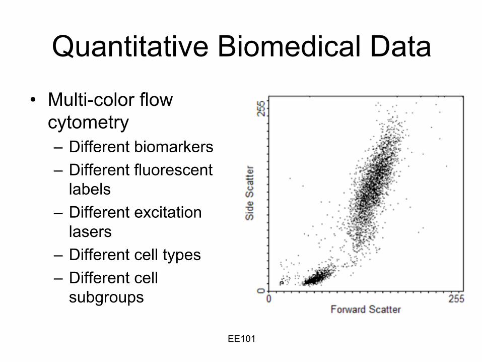
Quantitative Biomedical Data

•

Multi-color flow cytometry–

Different biomarkers

–

Different fluorescent labels

–

Different excitation lasers

–

Different cell types –

Different cell subgroups

EE101

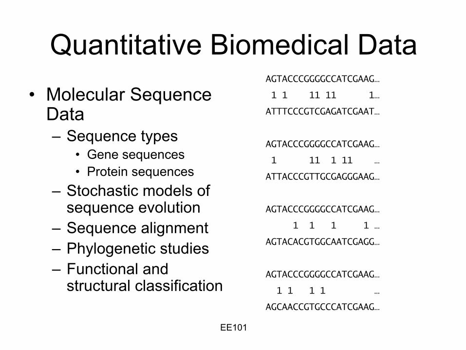
Quantitative Biomedical Data•

Molecular Sequence Data –

Sequence types

•

Gene sequences•

Protein sequences–

Stochastic models of sequence evolution

–

Sequence alignment–

Phylogenetic studies

–

Functional and structural classification

AGTACCCGGGGCCATCGAAG…

1 1 11 11

1…

ATTTCCCGTCGAGATCGAAT…

AGTACCCGGGGCCATCGAAG…

1 11 1 11 …

ATTACCCGTTGCGAGGGAAG…

AGTACCCGGGGCCATCGAAG…

1 1 1 1 …

AGTACACGTGGCAATCGAGG…

AGTACCCGGGGCCATCGAAG…

1 1 1 1 …

AGCAACCGTGCCCATCGAAG…

EE101

Example: Color Segmentation of H&E Stained Slides

•

Direct approach:–

Fit a three-component Gaussian mixture to a small random subset of histology Lab color data

•

small subset of ~10000 pixels for computational feasibility

–

Identify the three regions using the maximum likelihood rule

EE101

Example: Nuclei Detection on H&E Stained Histology Slides

•

Grayscale or color segmentation determines DNA-rich, stromal, and unstained region pixels

•

Nuclei detection is tantamount to detecting objects in a binarized

tissue segmentation maps with–

DNA-rich regions in the foreground–

Stromal

and unstained regions in the background•

Connected component labeling identifies the individual cell nuclei

original image DNA-rich region map

EE101

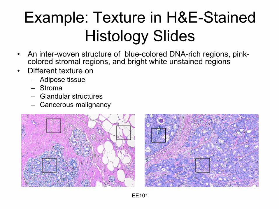
Example: Texture in H&E-Stained Histology Slides

•

An inter-woven structure of blue-colored DNA-rich regions, pink-

colored stromal

regions, and bright white unstained regions•

Different texture on–

Adipose tissue–

Stroma–

Glandular structures–

Cancerous malignancy

EE101

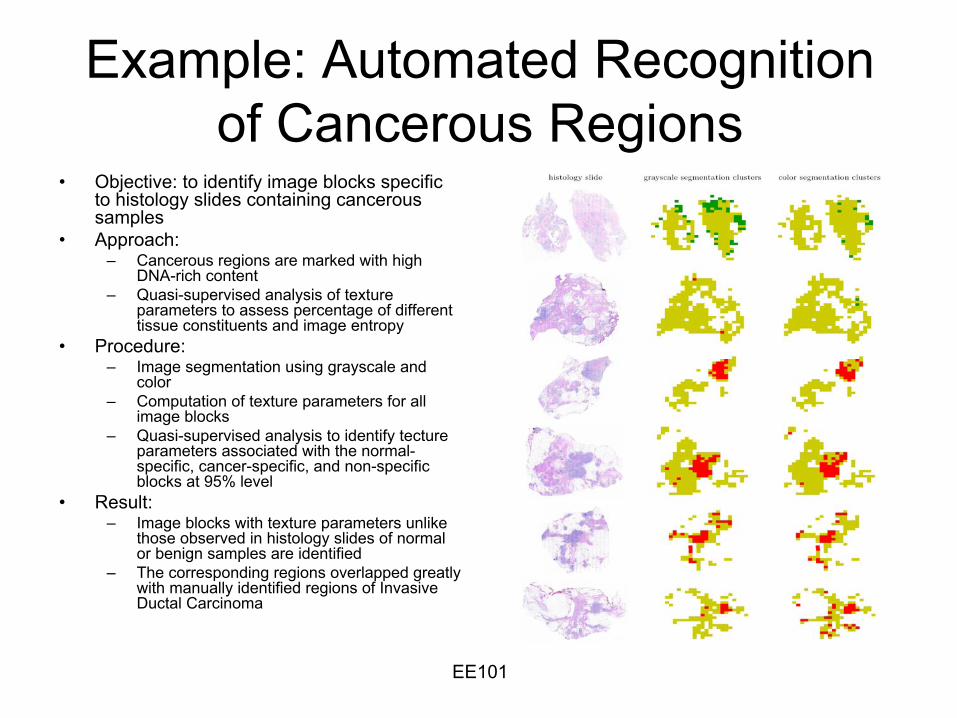
Example: Automated Recognition of Cancerous Regions

•

Objective: to identify image blocks specific to histology slides containing cancerous samples

•

Approach:–

Cancerous regions are marked with high DNA-rich content

–

Quasi-supervised analysis of texture parameters to assess percentage of different tissue constituents and image entropy

•

Procedure:–

Image segmentation using grayscale and color

–

Computation of texture parameters for all image blocks

–

Quasi-supervised analysis to identify tecture

parameters associated with the normal-

specific, cancer-specific, and non-specific blocks at 95% level

•

Result:–

Image blocks with texture parameters unlike those observed in histology slides of normal or benign samples are identified

–

The corresponding regions overlapped greatly with manually identified regions of Invasive Ductal

Carcinoma

EE101

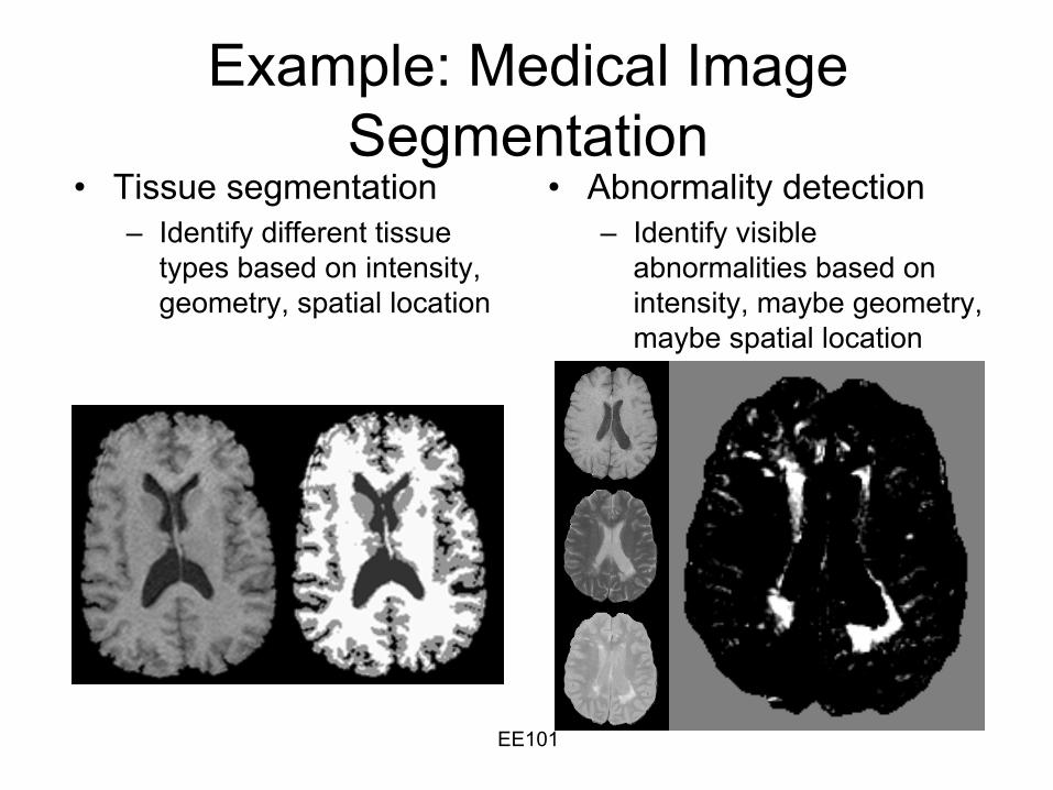
Example: Medical Image Segmentation

•

Tissue segmentation–

Identify different tissue types based on intensity, geometry, spatial location

•

Abnormality detection–

Identify visible abnormalities based on intensity, maybe geometry, maybe spatial location

EE101

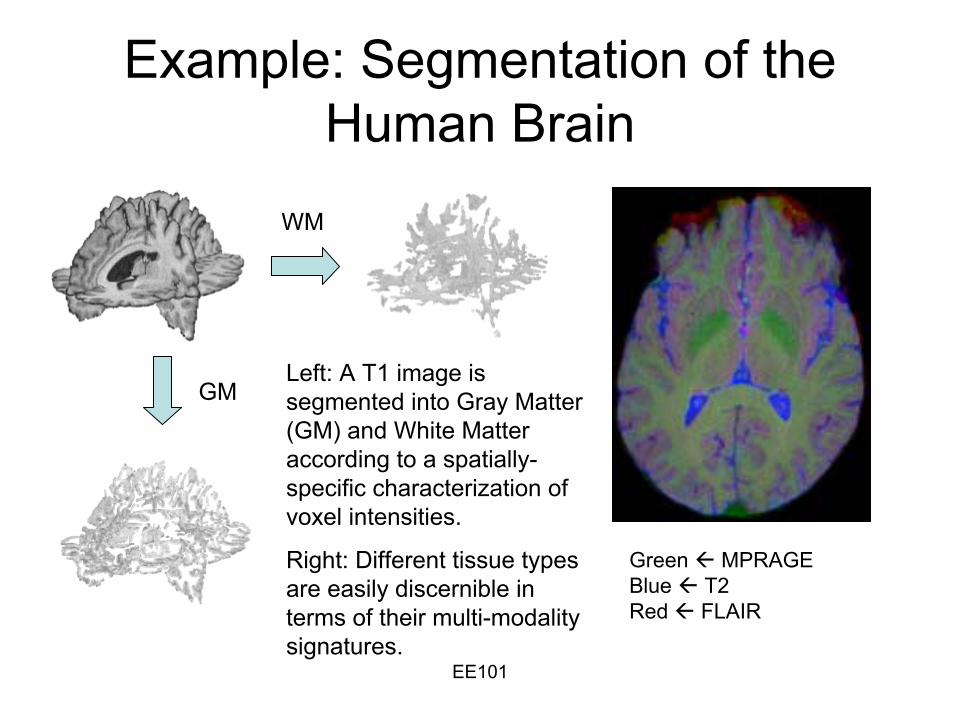
Example: Segmentation of the Human Brain

WM

GM

Green MPRAGEBlue T2 Red FLAIR

Left: A T1 image is segmented into Gray Matter (GM) and White Matter according to a spatially-

specific characterization of voxel

intensities.

Right: Different tissue types are easily discernible in terms of their multi-modality signatures.

EE101

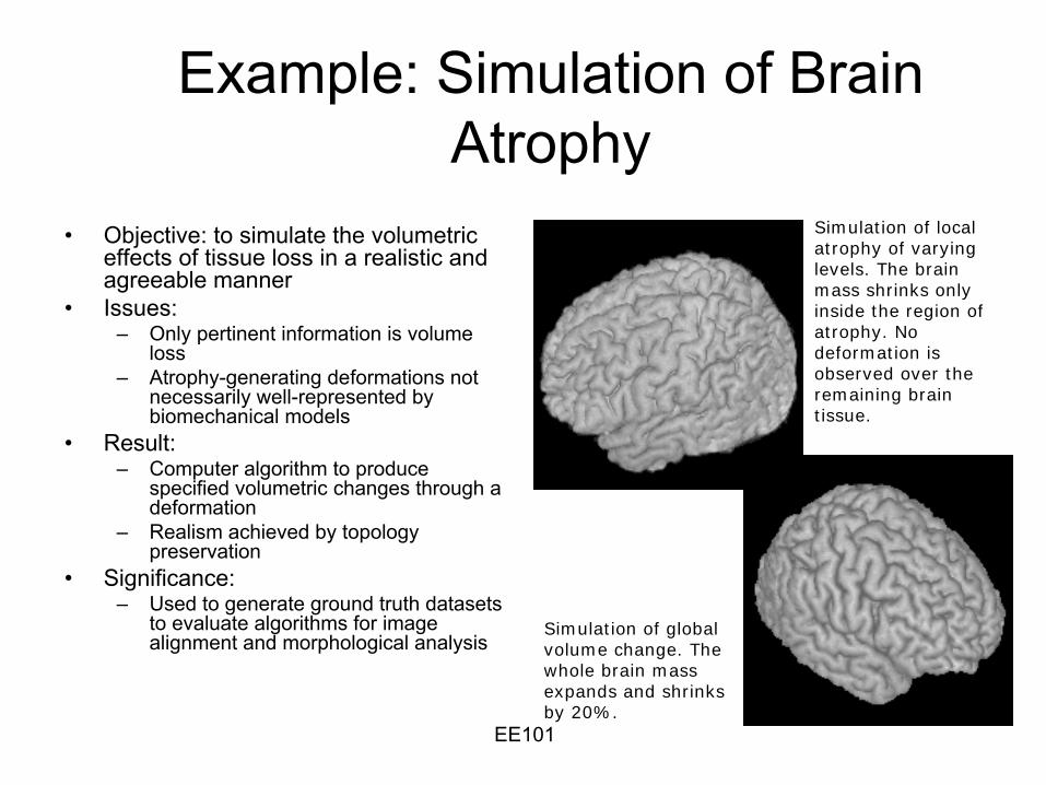
Example: Simulation of Brain Atrophy

•

Objective: to simulate the volumetric effects of tissue loss in a realistic and agreeable manner

•

Issues:–

Only pertinent information is volume loss

–

Atrophy-generating deformations not necessarily well-represented by biomechanical models

•

Result:–

Computer algorithm to produce specified volumetric changes through a deformation

–

Realism achieved by topology preservation

•

Significance:–

Used to generate ground truth datasets to evaluate algorithms for image alignment and morphological analysis

Simulation of local atrophy of varying levels. The brain mass shrinks only inside the region of atrophy. No deformation is observed over the remaining brain tissue.

Simulation of global volume change. The whole brain mass expands and shrinks by 20%.

EE101

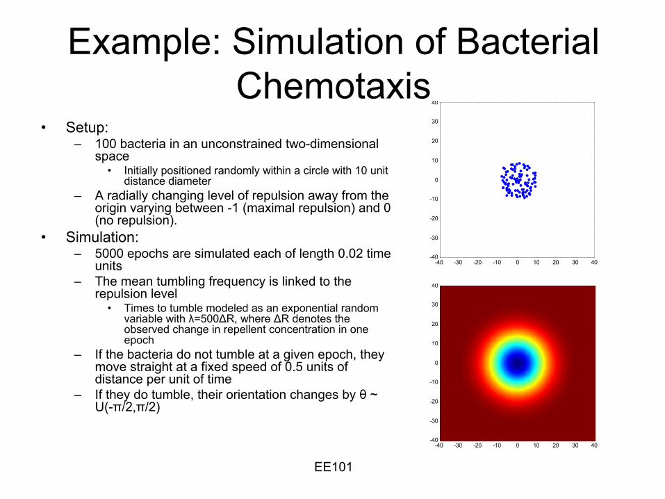
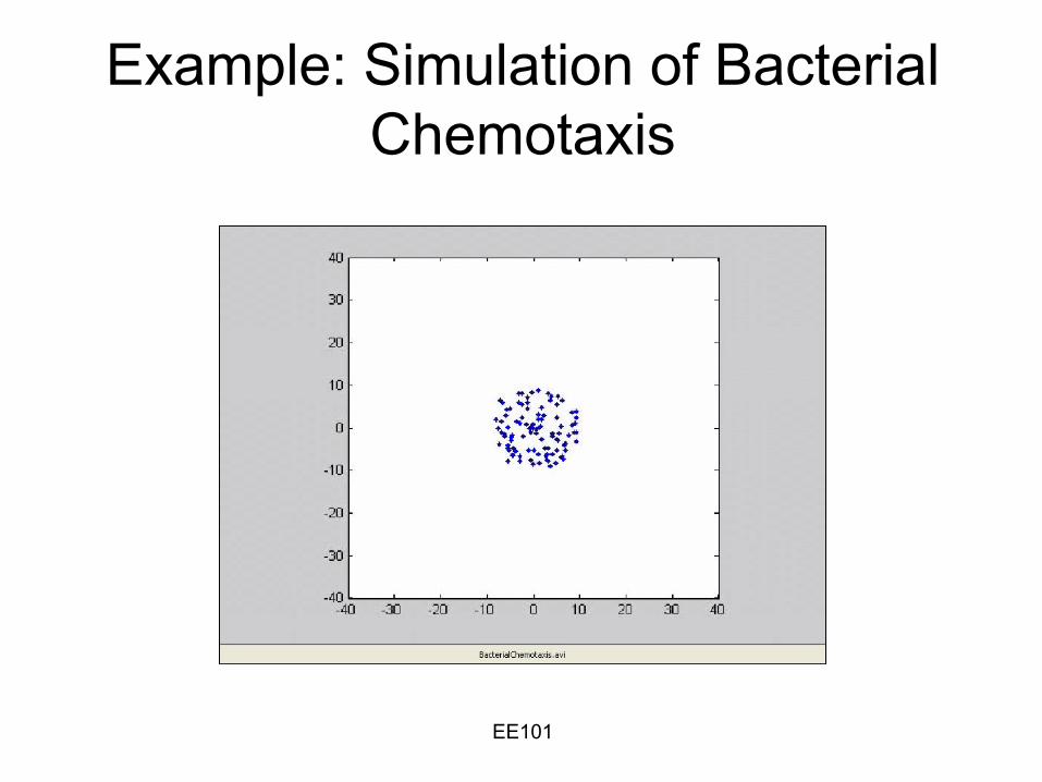
Example: Simulation of Bacterial Chemotaxis

•

Setup:–

100 bacteria in an unconstrained two-dimensional space

•

Initially positioned randomly within a circle with 10 unit distance diameter

–

A radially

changing level of repulsion away from the origin varying between -1 (maximal repulsion) and 0 (no repulsion).

•

Simulation:–

5000 epochs are simulated each of length 0.02 time units

–

The mean tumbling frequency is linked to the repulsion level

•

Times to tumble modeled as an exponential random variable with λ=500ΔR, where ΔR denotes the observed change in repellent concentration in one epoch

–

If the bacteria do not tumble at a given epoch, they move straight at a fixed speed of 0.5 units of distance per unit of time

–

If they do tumble, their orientation changes by θ

~ U(-π/2,π/2)

-40 -30 -20 -10 0 10 20 30 40-40

-30

-20

-10

0

10

20

30

40

-40 -30 -20 -10 0 10 20 30 40-40

-30

-20

-10

0

10

20

30

40

EE101

Example: Simulation of Bacterial Chemotaxis

EE101

Summary

•

Statistical signal processing techniques carry out all automated decision making tasks–

Detection

–

Recognition–

Classification

•

The basis of these techniques is an understanding of the random nature of the phenomenon of interest