editor in chief dr. kouroush jenab - university of malaya · improved irregular augmented ... we...
TRANSCRIPT


Editor in Chief Dr. Kouroush Jenab
International Journal of Engineering (IJE)
Book: 2008 Volume 2, Issue 3
Publishing Date: 30-06-2008
Proceedings
ISSN (Online): 1985-2312
This work is subjected to copyright. All rights are reserved whether the whole or
part of the material is concerned, specifically the rights of translation, reprinting,
re-use of illusions, recitation, broadcasting, reproduction on microfilms or in any
other way, and storage in data banks. Duplication of this publication of parts
thereof is permitted only under the provision of the copyright law 1965, in its
current version, and permission of use must always be obtained from CSC
Publishers. Violations are liable to prosecution under the copyright law.
IJE Journal is a part of CSC Publishers
http://www.cscjournals.org
©IJE Journal
Published in Malaysia
Typesetting: Camera-ready by author, data conversation by CSC Publishing
Services – CSC Journals, Malaysia
CSC Publishers

Table of Contents Volume 2, Issue 3, June 2008.
Pages
1 - 11
12 - 26
27 - 32
Analysis and Design Hilbert Curve Fractal Antenna Feed with Co-
planar Waveguide for multi-band wireless communications.
Niruth Prombutr, Prayoot Akkaraaektharin.
Enhancing the 'Willingness' on the OLSR Protocol to Optimize the
Usage of Power Battery Power Sources Left
Saaidal Razalli Azzuhri, Suhazlan Suhaimi, K. Daniel Wong.
Improved Irregular Augmented Shuffle Multistage Interconnection
Network
Sandeep Sharma, K.S.Kahlon, P.K.Bansal, Kawaljeet Singh.
33 - 40
41 - 50
Hybrid Optimization of Pin type fixture Configuration for Free Form
Workpiece
Afzeri, Nukhaie Ibrahim.
Purpose engineering for Contextual Role-Based Access Control
(C-RBAC)
Muhammad Nabeel Tahir.
International Journal of Engineering, (IJE) Volume (2) : Issue (3)

Niruth prombutr and Prayoot akkaraaektharin
International Journal of Engineering, Volume 2 Issue 31
Analysis and Design Hilbert Curve Fractal Antenna Feed withCo-planar Waveguide for multi-band wireless communications
Niruth Prombutr [email protected] of Engineering/Electrical engineering departmentMahidol UniversityNakornpathom,73170, Thailand
Prayoot Akkaraaektharin [email protected] of Engineering/Electrical engineering departmentKing Mongkut’s University of Technology North BangkokBangkok, 10800,Thailand
Abstract
There are many techniques to improve the characteristic of antennas. In thiswork we use ideas of the fractal. The purpose of this project is to design andanalyze Hilbert curve fractal antennas to get the empirical and electrical model.We use the Zealand program for simulating antennas. The antennas receive andtransmit in many frequency resonances. We design a small Hilbert curve fractalantenna. We analyze this antenna by using the concept of the CPW transmissionline and the mathematical definition of fractal to yield the models for Hilbert curvefractal antenna. From these models we can predict the multi resonancefrequency. In the experiment we found that the least percent of difference forelectromagnetics formular model with the experiment (0.4%) is lower than theleast of the difference for empirical model (4.43%) because the electromagneticsmodel used the transmission line model while the empirical model used thenumerical method. These models will be helpful for design and making Hilbertcurve fractal antenna.
Keywords: Fractal antenna, Multi-band, Hilbert curve, Electromagnetics model, Coplanar waveguid feed.
1. INTRODUCTIONThe term fractal was coined by the French mathematician B.B. Mandelbrot during 1970’s after hispioneering research on several naturally occurring irregular and fragmented geometries notcontained within the realms of conventional Euclidian geometry [1].The use of fractal geometrieshas significantly impacted many areas of science and engineering; one of which is antennas.Antennas using some of these geometries for various telecommunications applications arealready available commercially. The use of fractal geometries has been shown to improveseveral antenna features to varying extents. Yet a direct corroboration between antennacharacteristics and geometrical properties of underlying fractals has been missing. This researchwork is intended as a first step to fill this gap. In terms of antenna performance, fractal shapedgeometries are believed to result in multi-band characteristics and reduction of antenna size. Aquantitative link between multi-band characteristics of the antenna and a mathematicallyexpressible feature of the fractal geometry is needed for design optimization. To explore this, we

Niruth prombutr and Prayoot akkaraaektharin
International Journal of Engineering, Volume 2 Issue 32
design the Hilbert curves fractal antenna that use the coplanar wave guide feed. This has beenexplored numerically and validated experimentally. One of the advantages of using fractalgeometries in small antennas is the order associated with these geometries in contrast to anarbitrary meandering of random line segments (which may also result in small antennas).However this fact has not been used in antenna design thus far. In this work, approximateexpressions for designing antennas with these geometries have been derived incorporating theirfractal nature. To conclude, the research work reported here is a numerical and experimentalstudy in identifying features of fractal shaped antennas that could impart increased flexibility inthe design of newer generation wireless systems.Several antenna configurations based on fractal geometries have been reported in recent years[2] – [4]. These are low profile antennas with moderate gain and can be made operative atmultiple frequency bands and hence are multi-functional. In this work the multi-band(multifunctional) aspect of antenna designs are explored further with special emphasis onidentifying fractal properties that impact antenna multi-band characteristics. Antennas withreduced size have been obtained using Hilbert curve fractal geometry. Further more, designequations for these antennas are obtained in terms of its geometrical parameters such as fractaldimension. One of the fundamental advantages of using a fractal geometry in antennas isreducing the size of a resonant antenna. This is very evident in dipole and monopole antennasusing fractal Koch curves [5], and some of their modifications in the form of closed loops, andMinkowski curves [6]. The ability of these geometries to pack longer curves within relativelysmaller area is the salient aspect in their use in antennas. Being a plane filling geometry, Hilbertcurves can enclose longer curves for a given area than Koch curves [7].
2. Hilbert Curve Fractal antenna
2.1 Axioms L system for Hilbert CurveThe first few iterations of Hilbert curves are shown in Fig. 1. It may be noticed that eachsuccessive stage consists of four copies of the previous, connected with additional linesegments. This geometry is a space-Filling curve, since with a larger iteration, one may think of itas trying to fill the area it occupies. Additionally the geometry also has the following properties:self-Avoidance (as the line segments do not intersect each other), Simplicity (since the curve canbe drawn with a single stroke of a pen) and self-Similarity (which will be explored later). Becauseof these properties, these curves are often called an FASS curves [8].
FIGURE 1: First four iterations of Hilbert curve geometry.
The segments used to connect copies of the previous iteration are shown in dashed lines. Thegeneration algorithm of this geometry is commonly expressed in terms of L-systems. In thisrepresentation, a string of symbols with the following notations are used, leave two blank linesbetween successive sections as here.
(1)
(2)where is moving forward a step, + is turn left by , - is turn right by . A recursive approachmay be used to generate higher iterations ( is integer = 0, 1, 2, …) of the geometry from these

Niruth prombutr and Prayoot akkaraaektharin
International Journal of Engineering, Volume 2 Issue 33
(3)
(4)
2.2 Antenna Configurations Using Hilbert CurvesIt would be interesting to study the properties of a new antenna with reference to various existing,and more familiar antennas. In this context, a schematic of the thought process leading to theHilbert curve antenna. The half-wave meander line antenna is resonant when the arms areapproximately quarter wavelength long. The biconical antenna is a broadband variant for thecommon dipole [9]. This antenna can even be simulated with wires along its periphery. Puente etal [2] have used a bowtie as the base model for explaining the properties of the Sierpinski gasketfractal antenna with multi-band radiation characteristics.A conventional coplanar waveguide (CPW) on a dielectric substrate consists of a center stripconductor with semi-infinite ground planes on either side as shown in Fig 2. This type of antennaoffers several advantages over microstrip line. It simplifies fabrication, facilitates easy shunt aswell as series surface mounting of active and passive devices, eliminates the need for via holesand reduces radiation loss. In addition a ground plane exists between two adjacent lines; hencecross talk effects between them are very week. As a result, CPW circuits can be made denserthan microstrip circuits [9].
FIGURE 2: CPW antenna
CPW antennas are designed by using the IE3D program. This program has high efficiency,accuracy and low cost simulation tools. The proposed antenna is excited by a CPW line of 50and is fabricated on a FR4 substrate with a thickness (h) of 1.6 mm and relative permittivity ( ) of4.4. The two ground planes are placed symmetrically on each side of the CPW line. Design thefundamental resonance frequency at 1.8 GHz for the first stage of Hilbert curve antenna shown inFig 3.
a)

Niruth prombutr and Prayoot akkaraaektharin
International Journal of Engineering, Volume 2 Issue 34
b)FIGURE 3 : a) First stage of Hilbert curve geometry. b) the return loss of this stage
We design the next stage of this Hilbert curve antenna(stage 2, 3,and 4) and study the return lossresponse of each stage that shown in the Fig. 4,5 and 6 respectively. We found that the numberof resonance frequency increase that satisfy the concept of fractal antenna.
a)
b)FIGURE: 4 a) second stage of Hilbert curve geometry. b) the return loss of this stage
a)

Niruth prombutr and Prayoot akkaraaektharin
International Journal of Engineering, Volume 2 Issue 35
b)FIGURE: 5 a) third stage of Hilbert curve geometry. b) the return loss of this stage
a)
b)FIGURE: 6 a) fourth stage of Hilbert curve geometry. b) the return loss of this stage
3. Result
We made this Hilbert Curve antenna by using the fabrication on the FR-4 substrate that shown inFig. 7. The proposed antennas have been tested using a calibrated vector network analyzer.Measured result of the return loss(S11) compared with the simulation is shown in Fig. 8.
FIGURE: 7 The photograph of proposed Hilbert curve antenna at stage 4

Niruth prombutr and Prayoot akkaraaektharin
International Journal of Engineering, Volume 2 Issue 36
FIGURE: 8 Measured result of S11 compared with the simulation
The far-field radiation patterns of the proposed antenna have been measured by connectingtransmitting antenna to the frequency sweep generator and connecting the receiving antenna tothe spectrum analyzer. Measured results of the patterns had been plotted in Fig 9.
FIGURE: 9 Measured result of the patterns for the proposed CPW antennas
4 Analyze and Design formula
4.1 EMPIRICAL MODEL It is now possible to obtain approximate design equations for this type of antenna. The approachfor the design formulation is based on that followed for resonant meander line antennas [10].

Niruth prombutr and Prayoot akkaraaektharin
International Journal of Engineering, Volume 2 Issue 37
The resonant frequencies are obtained through the above formulation by use the numericalmethod. We can find the empirical model equation by using the basic concept of antenna thatstate the resonance frequency vary inversely with the size of the antenna as shown in the Fig. 10
FIGURE: 10 Dimension of Hilbert Curve Fractal Antenna iteration 4 at the first fourth resonance frequency.
From this design HCFA, the dimensions of antenna are h4=88 mm, h3=44 mm, h2=22 mm, andh1=7.266 mm. This antenna wills resonance at 0.84 GHz, 1.52 GHz 1.9GHz and 2.48 GHz thatsatisfy the size of antenna as shown in the table 1
n(band
)
fn(GHz) fn+1/
fn ( )
hn/ n
1 0.840 1.803 0.246
4
2 1.520 1.254 0.222
9
3 1.900 1.302 0.14
4 2.480 1.381 -
TABLE:1 The dimension of Hilbertcurve antenna at difference Resonance frequency
From the data we found that the ratio of the next stage resonance frequency to this stage willconverge to some number (1.38) that we call log period and the ratio of the height to theresonance wavelength seem to be constant about 0.21(average of 0.2464, 0.2229, 0.14) that weuse this coefficient in the proposed model. Finally the data has been analyzed resulting in anempirical model formula at resonance stage n
(5)where fn = the resonance frequency at stage n

Niruth prombutr and Prayoot akkaraaektharin
International Journal of Engineering, Volume 2 Issue 38
c= speed of electromagnetic wave= m/s h = the highest dimension size of antenna n = integer number at stage n (1,2,3,.,.)
= log period = 1.38
The resonance frequency from above model and simulation are compared with simulation. Atable of comparison is given below (Table 2). From the table, the percent of difference will besmaller at the higher resonance frequency. These antennas are fabricated on a FR4. Theseresults show a reasonable match between the simulation and empirical model, and hence it isconcluded that the above formulation may be used as an empirical design equation for antennasof this type.4.2 Electromagnetics Model
It is now possible to obtain approximate design equations for this type of antenna. The approachfor the design formulation is based on that followed for resonant meander line antennas [10]. Inthis approach, the inductances of the turns of the meander line are calculated, considering themas short circuited parallel-two-wire lines. The self inductance of an imaginary straight lineconnecting all these turns is then added to this to get the total inductance. This is then comparedwith the inductance of a regular half wavelength meander line. Since meander line antennas withapproximately half wavelength are resonant (their capacitive and inductive reactances canceleach other)[11], and assuming that the input capacitive reactance for a meander line antennaremains unchanged by reducing its apparent length by introducing turns, the resonant conditionfor this antenna is derived. The approach reported in [12] for the meander line meander lineantenna can readily be extended for the Hilbert curve antenna (HCA). The definition of selfinductance of a straight line for meander line antenna is replaced here with the total inductance ofthe line segments otherwise unaccounted (not forming short-circuited parallel wire sections).Another important assumption is that the capacitances of the meander line configurations remainthe same in all cases. For an HCA (Fig. 10) with outer dimension of and order of fractaliteration n, the length of each line segment d is given by
(6)
The number of short circuit terminations for parallel wire section be founded that
(7)
Niruth prombutr and Prayoot akkaraaektharin
International Journal of Engineering, Volume 2 Issue 39
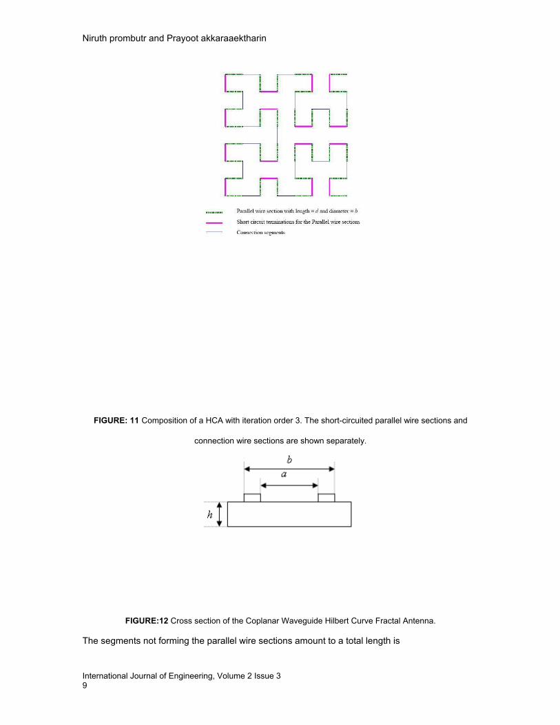
FIGURE: 11 Composition of a HCA with iteration order 3. The short-circuited parallel wire sections and
connection wire sections are shown separately.
FIGURE:12 Cross section of the Coplanar Waveguide Hilbert Curve Fractal Antenna.
The segments not forming the parallel wire sections amount to a total length is

Niruth prombutr and Prayoot akkaraaektharin
International Journal of Engineering, Volume 2 Issue 310
(8)
The approach we introduce to derive the condition for the resonant properties of Hilbert curveantennas printed on a dielectric substrate, is to consider sections of the strip as terminatedparallel strip transmission lines. The characteristic impedance of two parallel strips of negligiblethickness (t) printed on a dielectric of height (h), and dielectric constant , as shown in Fig.11 interms of complete elliptic integral of the first kind (K) is given by [12]:
(9)
where the effective dielectric constant is
and the pure inductance is
(10)The self inductance due to a straight line of length s as
(11)Substituting (9) in (10) and using (11), the total inductance is therefore
(12)It should however be noted that regular meander line antennas resonate when the arm length isa multiple of quarter wavelength. Thus, by changing the resonant length related terms on theRHS of equation, we can obtain all the resonant frequencies of the multi-band HCA. Thereforethe first few resonant frequencies of the HCA can be obtained from the formula model:
(13)where k is an odd integer (1,3,5,…) and
=propagation characteristics of the transmission line.The resonant frequencies were obtained through the above formulation by use the numericalmethod to iterate the frequencies that make the LHS equal RHS. The resonance frequency fromabove model and simulation were compared with experiments. A table of comparison is givenbelow (Table 2). From the table 2, these models will be more accurate at the higher frequency.These antennas are fabricated on a FR4. These results show a reasonable match between thetwo, and hence it is concluded that the above formulation may be used as an empirical designequation for antennas of this type.
Resonant Frequency(GHz)

Niruth prombutr and Prayoot akkaraaektharin
International Journal of Engineering, Volume 2 Issue 311
fr1 fr2 fr3Simulation 1.52 1.90 2.48
Empirical Model (Percentof Difference) 1.36 (10.52%) 1.87 (1.57%) 2.59 (4.43%)
Electromagnetics Model(Percent of Difference) 1.45 (4.6%) 1.96 (3.15%) 2.47 (0.4%)
TABLE: 2 Comparison of formulation with experimental simulation results for Hilbert curve antennas printed
5. ConclusionIn this work the development of antennas using Hilbert curve fractal geometry is presented.Some of the numerical results are validated through experiments and we found that the leastpercent of difference for this empirical model is 4.43%. The advantage of numerical method forthis work is easy because when we consider empirical model, this model gives the higherpercentage of difference than the electromagnetics model that gives the least percentage ofdifference for this model( 0.4 %). These models will be helpful for design Hilbert curve fractalantennas. The numerical results presented in this research indicate that further reduction inresonant frequency is possible for Hilbert curves. A patch configuration is also explored.However, the antenna characteristics in this configuration are found to be dictated by the outerdimensions.
6. References1. B.B. Madelbrot, The Fractal Geometry of Nature, New York: W.H. Freeman, 19832. C. Puente, J. Romeu, R. Bartoleme, and R. Pous, “Fractal multiband antenna based onSierpinski gasket,” Electron. Lett., vol. 32, pp. 1-2, 1996.3. C. Puente-Baliarda, J. Romeu, R. Pous, J. Ramis, and A. Hijazo, “Small but long Koch fractalmonopole,” Electron. Lett., vol. 34, pp. 9-10, 1998.4. N. Cohen, “Fractal antenna applications in wireless telecommunications,” in ProfessionalProgram Proc. of Electronics Industries Forum of New England, 1997,IEEE, pp. 43-49, 19975. C.P. Baliarda, J. Romeu, and A. Cardama, “The Koch monopole: A small fractal antenna,”IEEE Trans. Ant. Propagat., vol. 48 pp. 1773-1781, 2000.6. J.P. Glanvittorio and Y. Rahmaat-Samii, “Fractal element antennas: A compilations ofconfigurations with novel characteristics,” IEEE AP-S Inter. Symp. 2000, pp.1688-1691, 2000.7. V K.J. Vinoy, K.A. Jose, V.K. Varadan, and V.V. Varadan, “Hilbert curve fractal antenna: asmall resonant antenna for VHF/UHF applications,” Microwave & Optical Technology Letters, vol.29, pp. 215-219, 2001.8. H.-O. Peitgen, J.M. Henriques, L.F. Penedo (Eds.),”Fractals in the Fundamental and AppliedSciences”, Amsterdam: North Holland, 19919. Niruth Prombutr, Jarinthip Pakeesirikul, Theerayut Theatmongkol, Samuttachai Suangool,“Dual-band Coplanar Waveguide Antenna Design by using U-Slot with diagonal edge,” The 21stInternational Technical Conference on Circuits/Systems, Computers and Communications, vol III,pp 117-120, Chaingmai, 2006.10. T. Endo, Y. Sunahara, S. Satoh, and T. Katagi, “Resonant frequency and radiation efficiencyof meander line antennas,” Electronics & Commun. in Japan, Pt. 2, vol.83, pp. 52-58, 2000.11. C.A. Balanis, Antenna Theory: Analysis and Design, New York: John Wiley (2nd Ed.), 1997.12. B.C. Wadell, Transmission Line Design Handbook, Dedham Artech House, 1991.

Saaidal Razalli Azzuhri, Suhazlan Suhaimi & K. Daniel Wong
International Journal of Engineering, volume (2) issue (3) 12
Enhancing the 'Willingness' on the OLSR Protocol to Optimize the Usage of Power Battery Power Sources Left
Saaidal Razalli Azzuhri [email protected] Electrical Engineering Department, Faculty of Engineering University of Malaya Kuala Lumpur, 50603 Federal Territory, Malaysia Suhazlan Suhaimi [email protected] Faculty of Information & Communication Technology Sultan Idris Education University Tanjong Malim, 35900 Perak, Malaysia
K. Daniel Wong [email protected] Department of Information Technology Malaysia University of Science & Technology Petaling Jaya, 47301 Selangor, Malaysia
Abstract
Mobile ad-hoc networks are infrastructure-free and highly dynamics wireless networks. There are many routing protocols for Mobile Ad Hoc Networks (MANET). One of the popular routing protocols is Optimized Link State Routing (OLSR). OLSR was developed to work independently from higher-layer protocols and it creates an underlying architecture for communication without the help of traditional fixed-position routers. In addition, OLSR attempts to maintain the communication routes for the mobile nodes that have limited transmission range. This paper discusses the OLSR implementation in terms of battery power status and its advantages particularly pertaining to the relationship between the power status function with the OLSR by modify some of the OLSR source code. The study also focuses on maximizing the use of the battery power sources. The results from the experiment show that the usage of the battery power sources left was maximally used when the “Willingness” for the nodes was indeed increased. We will conclude that the experiments have been successfully done and the results demonstrate the improvement for the OLSR nodes to maximize the battery power sources usage on the MANET by enhancing the “Willingness” on the OLSR protocol. + Keywords: Multipoint-relay, ad-hoc, cross platform, OLSR, MANET
1. INTRODUCTION
A Mobile Ad Hoc Networks (MANET) is an autonomous system of mobile nodes. It consists of mobile platforms for example a router with multiple hosts and wireless communications devices. Herein simply referred to as 'nodes' which are free to move about arbitrarily. It also may operate in isolation or may have gateways to and interface with fixed network. There are many important

Saaidal Razalli Azzuhri, Suhazlan Suhaimi & K. Daniel Wong
International Journal of Engineering, volume (2) issue (3) 13
research questions in MANET. However, power efficiency is one of the most important issues. It is important to realize that issues such as QoS support, TCP performance, speed of routing repair process and others are secondary if nodes have a high probability of running out of energy resources. Energy awareness in wireless ad hoc networks actually spans across several communication layers. Advances in battery technology are very slow compared to the results achieved in integrated circuit technology particularly in comparison to the rate of growth in communication speeds. Therefore, saving transmission power represents one of the most significant methods for long term wireless system performance. In OLSR, the power energy resource is a very important factor in deciding whether the node can forward a packet or not. It is because only nodes where the “Willingness” is bigger than 7 can be used to forward packets. The higher the willingness of the node the higher the chance it will be selected as an MPR (we will explain the terms “willingness” and MPR later). The nodes willingness is based on the power resources it has from AC power sources or from the battery. There is no power problem when the nodes are using the power from the AC power sources as the nodes will get power consistently. However, problems may occur when the nodes use the power from the battery in which the power is limited. On the other hand, the MANET nodes are usually used in scenarios without any infrastructure, and therefore without AC power sources [1]. Thus, it is important to optimize the usage of the limited resources from the battery.
2. BACKGROUND THEORY 2.1. OPTIMIZED LINK STATE ROUTING (OLSR)
The Optimized Link State Routing Protocol (OLSR) is a protocol that was developed for mobile ad hoc network (MANET). It is a variation of traditional link state routing, modified for improved operation in ad hoc networks. It is a table driven and proactive routing protocol where the nodes exchange their topology information with other nodes regularly. The routes in the proactive protocols are always immediately available when needed [2]. OLSR is designed to work in a completely distributed manner and does not depend on any central entity. The protocol does not require reliable transmission of control messages. Each node sends control messages periodically and sustains a reasonable loss of some such messages. Such losses occur frequently in radio networks due to collisions or other transmission problems.
The key feature of this protocol is multipoint relays (MPRs). Topological changes cause floods of the topological information to all available nodes in the network. Therefore, the multipoint relays (MPRs) are used to reduce the overhead of network floods and size of link state updates. Every node selects a set of its neighbour nodes as multipoint relays (MPRs). Only MPRs nodes are responsible for forwarding control traffic. MPRs nodes only declare link-state information when the requirements for OLSR provide the shortest path information message [3]. The neighbours, whom the node selects as MPR, announce this information periodically in their ‘Control Message’. In route calculation, the MPRs are used to form the route from a given node to any destination in the network. It is also be used to facilitate efficient flooding of Control Message in the network. OLSR uses two kinds of Control Messages; Hello Messages and Topology Control messages.
2.1.1. HELLO MESSAGE
Each node should detect the neighbour nodes with which it has a direct and symmetric link. The uncertainties over radio propagation may make some links asymmetric. Consequently, all links MUST be checked in both directions in order to be considered valid. To accomplish this, each node broadcasts HELLO messages, containing information about neighbours and their link status. The link status may either be "symmetric", heard" (asymmetric) or "MPR". "Symmetric" indicates that the link has been verified to be bi-directional, for example, it is possible to transmit data in both directions. "Heard" indicates that the node can hear HELLO messages from a neighbour, but it is not confirmed that this neighbour is also able to receive messages from the node. "MPR" indicates that a node is selected by the sender as a MPR. A status of MPR further implies that the link is symmetric. These control messages are broadcast to all one-hop neighbours, but are *not relayed* to further nodes. A HELLO-message contains [4]:
• A list of addresses of neighbours, to which there exists a symmetric link.
Saaidal Razalli Azzuhri, Suhazlan Suhaimi & K. Daniel Wong
International Journal of Engineering, volume (2) issue (3) 14
• A list of addresses of neighbours, which have been "heard".
• A list of neighbours, which have been selected as MPRs. The list of neighbours in a HELLO message can be partial (for example, due to message size limitations, imposed by the network), the rule being that all neighbour nodes are cited at least once within a predetermined refreshing period (HELLO_INTERVAL).
2.1.2. TOPOLOGY CONTROL (TC) In order to build the topology information base needed, each node, which has been selected as MPR, broadcasts Topology Control (TC) messages. TC messages are flooded to all nodes in the network and take advantage of MPRs. MPRs enable a better scalability in the distribution of topology information. A TC message is sent by a node in the network to declare its MPR Selector set. For example, the TC message contains the list of neighbours which have selected the sender node as a MPR. The information diffused in the network by these TC messages will help each node to calculate its routing table. A node which has an empty MPR selector set, such as nobody has selected it as a MPR, MUST NOT generate any TC message.
2.1.3. CONTROL TRAFFIC
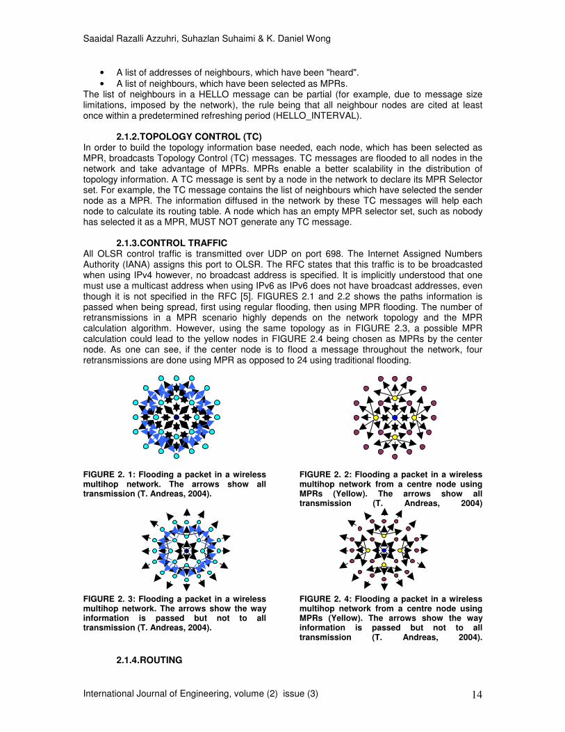
All OLSR control traffic is transmitted over UDP on port 698. The Internet Assigned Numbers Authority (IANA) assigns this port to OLSR. The RFC states that this traffic is to be broadcasted when using IPv4 however, no broadcast address is specified. It is implicitly understood that one must use a multicast address when using IPv6 as IPv6 does not have broadcast addresses, even though it is not specified in the RFC [5]. FIGURES 2.1 and 2.2 shows the paths information is passed when being spread, first using regular flooding, then using MPR flooding. The number of retransmissions in a MPR scenario highly depends on the network topology and the MPR calculation algorithm. However, using the same topology as in FIGURE 2.3, a possible MPR calculation could lead to the yellow nodes in FIGURE 2.4 being chosen as MPRs by the center node. As one can see, if the center node is to flood a message throughout the network, four retransmissions are done using MPR as opposed to 24 using traditional flooding.
FIGURE 2. 1: Flooding a packet in a wireless multihop network. The arrows show all transmission (T. Andreas, 2004).
FIGURE 2. 2: Flooding a packet in a wireless multihop network from a centre node using MPRs (Yellow). The arrows show all transmission (T. Andreas, 2004)
FIGURE 2. 3: Flooding a packet in a wireless multihop network. The arrows show the way information is passed but not to all transmission (T. Andreas, 2004).
FIGURE 2. 4: Flooding a packet in a wireless multihop network from a centre node using MPRs (Yellow). The arrows show the way information is passed but not to all transmission (T. Andreas, 2004).
2.1.4. ROUTING

Saaidal Razalli Azzuhri, Suhazlan Suhaimi & K. Daniel Wong
International Journal of Engineering, volume (2) issue (3) 15
LINK SENSING Link Sensing is accomplished through periodic emission of HELLO messages over the interfaces through which connectivity is checked. A separate HELLO message is generated for each interface and emitted in correspondence with the provisions. Resulting from Link Sensing is a local link set which describing links between "local interfaces" and "remote interfaces" for example the interfaces on neighbour nodes. If sufficient information is provided by the link-layer, this may be utilized to populate the local link set instead of HELLO message exchange. Link sensing populates the local link information base. Link sensing is exclusively concerned with OLSR interface addresses and the ability to exchange packets between such OLSR interfaces. The mechanism for link sensing is the periodic exchange of HELLO messages. The Link Set is populated with information on links to neighbour nodes. The process of populating this set is denoted "link sensing" and is performed using HELLO message exchange, updating a local link information base in each node. Each node should detect the links between itself and neighbour nodes. Uncertainties over radio propagation may make some links unidirectional. Consequently, all links MUST be checked in both directions in order to be considered valid. A "link" is described by a pair of interfaces: a local and a remote interface. For the purpose of link sensing, each neighbour node (more specifically, the link to each neighbour) has an associated status of either "symmetric" or "asymmetric". "Symmetric" indicates that the link to that neighbour node has been verified to be bi-directional, for example, it is possible to transmit data in both directions. "Asymmetric" indicates that HELLO messages from the node have been heard (for example, communication from the neighbour node is possible), however it is not confirmed that this node is also able to receive messages (for example, communication to the neighbour node is not confirmed). The information, acquired through and used by the link sensing, is accumulated in the link set. (A. Laoutti, P. Muhlethaler, A. Najid and E. Plakoo, 2002). The process will illustrate as a FIGURE 2.5.
FIGURE 2.5: A typical neighbour discovery session using HELLO message
MULTIPOINT RELAYS The Multipoint Relays (MPR) is the key idea behind the OLSR protocol in order to reduce the information exchange overhead. In OLSR only the MPRs can forward the data throughout the network. Each node must have the information about the symmetric one hop and two hop neighbours in order to calculate the optimal MPR set. The two hop neighbours are found from the Hello message because each Hello message contains all the nodes’ neighbours [7]. FIGURE 2.6 shows the multipoint relays (MPRs) selection between its neighbours. For instance node A select m1, m2 and m3 nodes. When node A floods a message, only node m1, node m2 and nod m3 re-transmit it, after that the MPRs of node m1, node m2 and node m3 retransmit and so on. There are 2 rules to select a node for MPR:
• First, any 2-hop neighbour must be covered by at least one multipoint relay.
• Second, try to minimize the number of multipoint relays. Then a node forwards a flooding packet according to several rules. The multipoint relays idea is to reduce the redundant retransmissions in the same region by minimizing the overhead of flooding message in the network. Each node in the network selects a set of nodes in its symmetric 1-hop neighbourhood, which may retransmit its messages. This set of selected neighbour nodes is called the "Multipoint Relay" (MPR) set of that node. The neighbours of node N which are *NOT* in its MPR set, receive and process broadcast messages but do not retransmit broadcast messages received from node N.

Saaidal Razalli Azzuhri, Suhazlan Suhaimi & K. Daniel Wong
International Journal of Engineering, volume (2) issue (3) 16
Each node selects its MPR set from among its 1-hop symmetric neighbours. This set is selected such that it covers (in terms of radio range) all symmetric strict 2-hop nodes. The MPR set of N, denoted as MPR (N), is then an arbitrary subset of the symmetric 1-hop neighbourhood of N, which satisfies the following condition: every node in the symmetric strict 2-hop neighbourhood of N must have a symmetric link towards MPR (N) (FIGURE 2.7). The smaller a MPR set, the less control traffic overhead results from the routing protocol gives an analysis and example of MPR selection algorithms.
FIGURE 2.6: The Selection of MPRs among its
neighbours.
FIGURE 2.6: Symmetric strict 2-hop
neighbours of node A
Each node maintains information about the set of neighbours that have selected it as MPR. This set is called the "Multipoint Relay Selector set" (MPR selector set) of a node. A node obtains this information from periodic HELLO messages received from the neighbours. A broadcast message, intended to be diffused in the whole network, coming from any of the MPR selectors of node N is assumed to be retransmitted by node N, if N has not received it yet. This set can change many time (for example, when a node selects another MPR-set) and is indicated by the selector nodes in their HELLO messages. Another rule that apply here is re-emitting rule that is shown in FIGURE 2.8. In FIGURE 2.8, if node m5 receives from node m2 first, it will re-transmit but, if the node m5 receives from node m1, it will not re-transmit. It means that no node will be missed when OLSR is used. SHORTEST PATH WITH MPR LINKS The MPR links offer a sparse partial topology containing the shortest paths. Any 2-hop neighbour of n node of a source of A node must have selected by some neighbours of A node as a MPR since an A node is a 2-hop neighbour of n node. Indeed, any node at distance m6 node from A node must have selected as MPR. Thus, it used MPR links backward to route from A node to m6 node.
FIGURE 2.7: Re-emitting rule
FIGURE 2.8: The shortest path with MPR link

Saaidal Razalli Azzuhri, Suhazlan Suhaimi & K. Daniel Wong
International Journal of Engineering, volume (2) issue (3) 17
TOPOLOGY ADVERTISEMENT IN OLSR The MPR links are flooded in every node. Every node is able to compute the shortest path routes to every destination. On the other hand classical link state protocols will flood entire neighbourhoods, consuming additional bandwidth for just getting redundant routes. A) MULTIPOINT RELAYS SELECTION The objective of MPR selection is for a node to select a subset of its neighbours such that a broadcast message, retransmitted by these selected neighbours, will be received by all nodes 2 hops away. The MPR set of a node is computed such that it, for each interface, satisfies this condition. The information required to perform this calculation is acquired through the periodic exchange of HELLO messages, as described in section 6 in the RFC 3626. The MPR Selections algorithm that propose by RFC 3626 constructs the MPR set which includes minimum number of the one hop symmetric neighbours from which it is possible to reach all the symmetrical strict two hop neighbours. The node must have the information about one and two hop symmetric neighbours in order to start the needed calculation for the MPR set. All the exchange of information is broadcasted using Hello messages (H. Aleksandr, 2004). B) TOPOLOGY SELECTION The nodes that are selected as MPR need to send the topology control (TC) message in order to exchange and build topological information base. Only MPRs are allowed to forward TC messages, in which TC messages are broadcasted throughout the network. In order to advertise its own links, TC message must be sent by a node in the network. The node must send at least the links of its MPR selector set. The TC message includes the own set of advertised links and the sequence number of each message. The sequence number is used to avoid loops of the message, if the node gets a message with the smaller sequence number, it must discard the message without any updates. The node must increment the sequence number when the links are removed and added from the TC message (H. Aleksandr, 2004). When the nodes advertised, links set becomes empty and it can still send an empty TC messages for specified amount of time, in order to invalidate previous TC messages. The size of the TC message can be quite big, so the TC message can be sent in parts during some specified amount of time. Node can increase its transmission rate to become more sensible to the possible link failure. C) ROUTING TABLE CALCULATION The node maintains the routing table in which the routing table entries have “destination address”, “next address”, “number of hops” to the destination address and “local interface address”. “Next address” indicates the next hop node. The information can be get from the topological set (TC messages) and the local link information base (Hello messages). Therefore, any changes for the set, the routing table will be recalculated (P. Jacquet, A. Laouitti, P. Minet and C. Viennot, 2001).
2.2. MULTIPOINT RELAY ( MPR COMPUTATION ) The detail description that specifies a procedure of the proposed heuristic and the terminology that used to describing the heuristic will get in RFC 3626 document for selection of MPRs. It constructs a MPR-set, which enables a node to reach any node in the symmetrical strict 2-hop neighbourhood through relaying on one MPR node with willingness that is different from WILL_NEVER. The heuristic MUST be applied per interface. The MPR set for a node is the union of the MPR sets found for each interface. The implementation of the algorithm is located in /src/mpr.c which is the mpr.c source code file was automatically installed when installing the OLSR software. All one-hop neighbours are linked to the two-hop neighbours that can be reached. Therefore, when selecting a neighbour as MPR, all corresponding two-hop neighbours can easily be updated to reflect this. The algorithm removes all previous selected MPRs and recalculates the whole MPR set. This is done by traversing the neighbour set based on the registered willingness of neighbours, starting with a willingness of 7 and decreasing down to 1. Nodes with a willingness of 0(WILL_NEVER) are never selected as MPRs wile nodes announcing a willingness of 7(WILL_ALWAYS) will always be selected as MPRs.

Saaidal Razalli Azzuhri, Suhazlan Suhaimi & K. Daniel Wong
International Journal of Engineering, volume (2) issue (3) 18
2.3. WILLINGNESS (SETTING WILLINGNESS) “Willingness” is a willing or interest of the node in the Ad Hoc network to give a contribution or commitment to the other nodes in order to send a data in the network. In OLSR, willingness is set based on the power-status of the node. This information is extracted from the pseudofile /proc/apm, which is the user-space interface to the Advanced Power Management offered by the kernel. Advanced Power Management (APM) is the predecessor to ACPI. The BIOS needs to handle all power management which devices are being set into lower power status based on the device activity timeouts. In this case, if no such file is present, willingness will be set to WILL_DEFAULT (3). The user can also set a fixed value for willingness in the configuration file. The willingness is based on a trivial calculation. Beneath is the snippet of code that calculates willingness. This code is implemented in the function “olsr_calculate_willingness” in src/olsr.c. This olsr.c source code file was installed automatically into the nodes computer when doing the installation of the OLSR software.
FIGURE 2.9: Source code for “olsr_calculate_willingness” function in olsr.c source code file
FIGURE 2.10: The willingness calculation flow diagram
2.4. OLSRD PLUG-IN
In order to maintain the communication session, process and generate packets, OLSR allows the usage of dynamically linked plug-ins, which is able to access the necessary functionality in it. Plug-ins can be used for almost everything because the plug-in interface offers a multi-purpose call to perform its specialized tasks. The OLSR daemon (olsrd) is support dynamic loading of plug-in (dynamic link library) for generation and processing of private package type starting from the version 0.4.3. The OLSR version that we used on the experiment was version 0.4.10. The design has been chosen because it does not need to change any code in olsrd in order to add custom package of functionality. The plug-in also can be written with any languages that can be compiled as a dynamic library. Thus, a person does not need to use the extended OLSR functioning to rely on heavy patching in order to maintain functionality whenever the new olsrd version is released.
2.5. THE POWERSTATUS PLUG-IN
The powerstatus plug-in provides a function where the node periodically floods the network with a custom packet, containing the following information:
• Whether or not the node is battery powered
• Estimated usage time left on the battery if using a battery
• Percentage of power left on the battery if battery powered. It is very useful to inform the other nodes about the status of the power info itself. This information is very useful for the node to calculate the willingness for the usage of the other node to select a MPR. The details about the MPR and willingness have been discussed earlier of this chapter.
3.0 METHODOLOGY 3.1. RESEARCH TOOLS
We use specific tools for doing the experiments such the operating system, hardware, software

Saaidal Razalli Azzuhri, Suhazlan Suhaimi & K. Daniel Wong
International Journal of Engineering, volume (2) issue (3) 19
and also the environment of the testbed. We need to verify the specific tools because the different tools that we used sometimes give some effect to the result that we collect. It is also important because we need to make sure that all the element that we used for the tools are applicable and can work well without any error.
3.1.1. OPERATING SYSTEM REQUIREMENTS The platform used Linux operating system (Fedora Core 5 and 6) in the experiment because the updated development of OLSR was created on it. In order to make sure the OLSR software could work with the latest Linux operating system, the latest version of Linux was chosen for experiment ensuring the required capabilities. Thus, the latest Linux kernel version (version 2.6.19) was used in the experiments ensuring that the results from the experiments are reliable.
3.1.2. HARDWARE REQUIREMENTS
In order to achieve greater mobility, wireless notebook devices were used to perform the OLSR functions. Other devices such as PDAs or hand phones are also suitable with OLSR depending on the operating system that supports the hardware. For this testbed, three DELL’s notebooks Latitude D500 named as Telco1, Telco2 and Telco3 are been used. Another notebook that has been used in the experiment was Acer Aspire 5580, which was given the name Acer. The detail of the specifications and configurations is shown in TABLE 3.1.
TABLE 3. 1: The hardware specification and configuration for OLSR nodes.
3.1.3. SOFTWARE REQUIREMENTS
The experiments used the latest version of the OLSR in the implementation of the testbed utilizing the olsrd-0.4.10 version. There are a lot of enhancements in OLSR, entailing the use of the latest version that is free from bugs compared to the previous version. Therefore, the latest version is better and more reliable for use in the experiment owing to its latest features of OLSR software. The ‘gcc’ (gnu c compiler) is one of the prerequisite software for the OLSR that should be installed in the Linux for OLSR software compilation. Others software or tool the used was wireshark software, ping and traceroute or tracert tools.
3.1.4. TESTBED REQUIREMENT
This experiment was tested on MUST campus environment, which involved the first floor and second floor of wing C comprising the Wireless room, IT lab, library and the corridor in the first and second floor for testbed. The results would differ if the experimental requirements chosen were altered.
3.2. OLSR SOURCE CODE MODIFICATION The focus of the experiment is on maximizing the battery usage and the OLSR performance namely the modification of the core and the power status plug-in on the OLSR software to determine the change of willingness that relate to the usage of power resources based on the AC power or battery power sources. At this juncture, the willingness can be enhanced and upgraded in order to maximize the usage of the resources especially when the node is using the battery power sources. FIGURE 2.11 in Chapter 2 summarizes the flow of the willingness calculation, which includes the Core OLSR function and the power status plug-in on OLSR. In the basic OLSR core, only the default and manual willingness setting for the node itself is available. On the

Saaidal Razalli Azzuhri, Suhazlan Suhaimi & K. Daniel Wong
International Journal of Engineering, volume (2) issue (3) 20
other hand, the power status plug-in is where the willingness calculations are performed. The plug-in also has the function as the source of the power information that will be broadcasted into the network where the information will be picked by other node in order to know the power status of the other nodes. The default value that is set in the core OLSR implementation is 3 because the information from the /proc/apm file is not available. The node may use the power source either using the AC or battery power. In this case, other nodes could not know the status and information about the node and for safety purpose; the willingness is set to the value of 3 because if the node uses the weak battery power, the network would automatically lose it without any warning invariably affecting the network to lose data. Alternatively, the setting can be based on user needs if they do not want to install power status plug-in with set the willingness to default or set the value (1-3 value) at the olsrd.conf file in order to allow the information for the node of the power status known to other devices. The willingness calculation on the other hand is located at the power status plug-in. The information flows to the power status plug-in function and then it will be calculated. The value of the willingness will be calculated when the usage of the AC power sources is 6. While the willingness value 1-3 indicating the percentage of balance of the battery power source. The values that have been calculated are not efficient because the resource is not consumed maximally. However, it has to maximize the usage of the power sources particularly in emergency situations such as natural disaster, fire, and earthquake and also for the military operations. Therefore, it is proposed that the value is change from 6 (old willingness value) to 7 (new willingness value) when using AC power because the source can get the power consistently. When using the battery power source, the value change from 1 - 3 (old willingness value) to 0 – 7 (new willingness value), thus increasing the granularity of the possible values and maximizing the resources available to the nodes. The main reason for optimizing the power resource and willingness are to make sure all nodes have enough battery power resource in which the battery is limited and it have more chances to be selected as MPR. The details of the MPR are summarized in the FIGURE 3.1 below.
FIGURE 3.1: The new value for the willingness calculation flow diagram
3.3. OLSR INSTALLATION WITH POWER STATUS PLUG-IN SOFTWARE.
In default, the willingness value is automatically derived from the core OLSR software without the calculation of the willingness. However, it does not use the power status information from the /proc/apm file. It only uses either the default value that have been set or the value from the user setting. The willingness calculation function is located at the power status plug-in where the plug-in is not installed by default with the OLSR software during the installation. The power status plug-in should be installed manually when the user needs to optimize power utilization with OLSR. The OLSR software can work well if the power status plug-in is not installed and A/C power is used, but the results of such OLSR experiments are not highly reliable because it does not replicate the real situation. In real ad hoc network, sometimes there is no infrastructure and it needs the power status function to calculate the willingness based on the information from the /proc/apm file [8].

Saaidal Razalli Azzuhri, Suhazlan Suhaimi & K. Daniel Wong
International Journal of Engineering, volume (2) issue (3) 21
4.0 SETUP AND INSTALLATION
4.1. INTRODUCTION The OLSRd software started out as part of the Master thesis project for Andreas Tonnesen at the University Graduate Centre. The OLSRd project is still on-going while the Master thesis has reached its completion. All nodes must be capable to detect and communicate with each other to establish a network where the infrastructure does not exist or where the services are not required. The IEEE 8102.11 Ad-hoc mode does not support multihop communications, whereas OLSR does. In the OLSR testbed, the Acer node could talk to Telco3 node through Telco2 node where the Acer node and Telco3 node were out of range (radio). The FIGURE 4.1 illustrates the testbed implemented in the experiment.
FIGURE 4.1: Multihop on OLSR
4.2. OLSR INSTALLATION
The nodes of the OLSR testbed were setup using Fedora Core 5 and Fedora Core 6 with the latest update kernel 2.6.19. It involved four notebooks that were installed with the OLSR software. The OLSR software can be downloaded through the internet at www.olsr.org web site. The source files were tarred using tar and bzipped using bzip2. This experiment used the release source which was 0.4.10. Then, after extracting the file, it was compiled and installed after browsing and achieving it. After the compilation and installation was complete, the olsrd.conf file, which is located at /etc/olsrd.conf was configured. All nodes are configured with the static IP address (and they must be, since there is no DHCP server to provide a dynamic address).
4.3. NETWORK CONFIGURATION ON OLSR
OLSR nodes must get the latest update kernel of the Linux operating system (Fedora Core 5 and 6) from the ftp site and it also must been installed with gcc. The gcc in Linux is used to compile the source code after performing the changes of the OLSR source code. The wireless interface on each node should be configured with an IP address. The nodes should be configured with the same ESSID. The wireless card should be configured with “ad-hoc” mode. The other thing that is compulsory is to release the UDP/698 from blocking. When all the networks have been configured, the next step is to configure the olsrd.conf file. The main option that has to change is the debug level (0 – 9) which can be seen through the process where the daemon runs. Next is the IP version, and in this case it uses IPv4. Lastly, it will configure the wireless interface under the name “eth1”. More details about the configuration can be found in the olsrd.conf document. The configuration can be enhanced depending on the needs of a user. The basic configuration needs on the olsrd.conf file is shown in Figure 4.2. The interfaces for the wireless are different for each other ensuring that the interface, which was already set at the olsrd.conf file, is correct. Then, the interface could be checked by using the command code at the terminal windows. Therefore, the tests that were planned performed well representing a small scale of the network (FIGURE 4.3).

Saaidal Razalli Azzuhri, Suhazlan Suhaimi & K. Daniel Wong
International Journal of Engineering, volume (2) issue (3) 22
FIGURE 4.2: The network configuration and
olsrd.conf file for OLSR nodes.
FIGURE 4.3: OLSR network communicate
On the other hand, the OLSR network can also be connected to the hard-wired (Ethernet) connection for a large network as well as network interface running on OLSR. It uses the Node and Network Association (HNA) message that contains sufficient information for the recipients to construct an appropriate routing table enabling the HNA (for IPv4 or IPv6) in the olsrd.conf file (FIGURE 4.5). FIGURE 4.4 illustrates the OLSR connection with the large fix connection.
FIGURE 4.4: OLSR connection with large fix
network.
FIGURE 4.5: The HNA configuration on
olsrd.conf file.
4.4. INSTALLATION THE PLUG-IN ON OLSR The OLSR nodes were actually connected to each other without knowing the power status of the default node. It is actually optional for the OLSR to work without the power status function. In this experiment, the power status plug-in that has been provided with the OLSR source code file would be used during the downloading and installing process into the nodes. On the other hand, this function was not installed into the node when installing the OLSR automatically. Hence, it must be installed manually because it is optional for the OLSR as it is not a core function. The Power Status plug-in locates the olsrd library directory when the OLSR is installed into the computer. It uses the Make and Make Install commands to compile and install the power status function. When the compilation and the installation of the OLSR are complete, it must configure the olsrd.conf file as shown in Figure 4.6 below.
Acer / Telco 1 / Telco2 / Telco3
/etc/sysconfig/network_scripts/ifcfg-eth1
…
MODE=Ad-Hoc
ESSID=olsr
CHANNEL=1
RATE=11M
/etc/olsrd.conf
DEBUG 3
IPVERSION 4
…
INTERFACE “eth1”
{...
Ip4Broadcast 255.255.255.255
…}
Acer / Telco2 / Telco3
/etc/olsrd.conf
DEBUG 3
IPVERSION 4
…
Hna4
{
…
}
…
INTERFACE “eth1”
{
...
Ip4Broadcast 255.255.255.255
…
}

Saaidal Razalli Azzuhri, Suhazlan Suhaimi & K. Daniel Wong
International Journal of Engineering, volume (2) issue (3) 23
FIGURE 4.6: Adding the plug-in script olsrd.conf file
The “olsrd_power.so.0.3” would be located at the /usr/lib/ after the power status installation. It should be located at the correct path because it would show the error and the OLSR automatically terminates (stops) when it runs the OLSR. It must also have the open and close curly bracket after the plug-in function. Once completed, the OLSR network should be tested to determine whether an error has occurred or not.
5.0 NETWORK ANALISYS When all the modifications were completely compiled, we next tested the resulting version on the network and collected some result from the OLSR deployment. The data collection only focuses on the availability of the nodes and also on the routing of the nodes on the ad-hoc network. This is because, the focus of the modification is to make sure the node on the OLSR is selected as MPR and to make sure the node is transferring the data willingly on the ad-hoc networks by using the limited battery power sources. Theoretically, the original OLSR source is calculating the percentage of the battery power balance and the willingness that can be acquired as summarized in FIGURE 5.1 and the modification of the OLSR source is summarized in FIGURE 5.2 as below.
FIGURE 5.1: The percentage (%) of battery power balance with the willingness assign (original source)
FIGURE 5.2 : The percentage (%) of battery power balance with the willingness assign (modification source)
Based on FIGURE 5.1 and FIGURE 5.2, comparison of the “Willingness” between the sources is illustrated in TABLE 5.1. The “Willingness” value based on the percentage (%) of battery power left is shown in Figure 5.7.
/etc/olsrd.conf
DEBUG 3
IPVERSION 4
…
LoadPlugin “/usr/lib/olsrd_power.so.0.3”
{
}
…
INTERFACE “eth1”
{...
Ip4Broadcast 255.255.255.255
…}

Saaidal Razalli Azzuhri, Suhazlan Suhaimi & K. Daniel Wong
International Journal of Engineering, volume (2) issue (3) 24
TABLE 5.1: The willingness comparison table between original and modification sources
FIGURE 5.3: The comparison table on the willingness for original and modification sources based on the percentage of battery power left.
FIGURE 5.3 shows that the willingness for the modified source code is better than the original source code until the percentages of the battery power available reached 20% level. Then, the percentages of battery dropped from 12.5% to 0%, where the “Willingness” was set to 0, in order to give the node enough time to shutdown properly saving all the works being performed. TABLE 5.1 and FIGURE 5.3 show that the “Willingness” on the OLSR plays an important role in choosing a node as MPR. OLSR availability During the experiment on the OLSR ad-hoc network, the network itself must be available. It will affect the OLSR ad-hoc network if the nodes on that network were not available. It will also become a major factor in the measurement performance for the OLSR ad-hoc network. To test the availability of the nodes, “Ping” is used to check either the nodes are available or not on the network. In this experiment, four notebook computers were used for checking the OLSR availability. The details on the hardware and software specifications have been discussed in CHAPTER 3, in which the nodes setup is illustrated in FIGURE 5.4 overleaf.
FIGURE 5.4: OLSR networking topology
5.1. USING AVAILABILITY STATISTIC DURING OLSR EXPERIMENT
When multiple ping packets are sent to a remote node, the ping program tracks on how many responses are received. The result will display as the percentage of the packets, which is not received. A network performance tools can use the “ping” statistic to obtain basic information regarding the status of the networks between the two end points. Once it is confirmed that there are lost packets in the “ping” sequence, it must determine the cause of the packet loss either due to the collisions on network segment or the packet being dropped by a network device. In the experiment, there was no packet loss on the OLSR networks.

Saaidal Razalli Azzuhri, Suhazlan Suhaimi & K. Daniel Wong
International Journal of Engineering, volume (2) issue (3) 25
5.2. ROUTING TABLE When the network in all the OLSR nodes were available and all of them were communicating each other, the Telco3 node then moved far away from Ftec node until the node was out of range of the Ftec node. This is because the Telco3 node must use either the Telco1 or the Telco2 node in transferring the data to the Ftec node and vice versa. In the experiment, the setup of the nodes was performed as illustrated in FIGURE 5.16. 1. Ftec node (10.0.1.4) was located at the wireless room in the IT lab. Telco2 node (10.0.1.2)
and Telco1 node (10.0.1.1) were located in the IT Lab near the door. All the three nodes were on the first floor situated on the left side of Wing C.
2. Telco3 node (10.0.1.3) was located on the second floor, in front of the lecture rooms, which was far away from Ftec node (10.0.1.4). Both nodes were out of line-of-sight range from one another. In this case, both nodes could only communicate via Telco1 or Telco2 node.
However, it needed to collect the data for analysis from the routing table for Ftec node and Telco3 node using a “traceroute” for Fedora Core 5 and “tracert” for Fedora Core 6. This experiment was performed based on time frame to get better result. The result shows that the Ftec node (source node) chose Telco2 node to transmit the data to the Telco3 node (destination) and the Telco3 node (source node) chose Telco2 node to transmit the data to Ftec node (destination node). Therefore, Telco2 node was selected as MPR because the value of the willingness was higher than telco1.
5.3. SUMMARY FROM THE EXPERIMENT The result shows that the willingness plays an important role in choosing a node as MPR in OLSR Ad Hoc network. The higher value of the willingness of the node, the more possibility of that node to be chosen as MPR. The lower value of the willingness of the node, the lower the possibility of the node to be chosen as MPR. On the other hand, if all nodes have almost the same of the less value, then the MPR will be chosen according to the highest value among the nodes. However, the results will be different if the experiment involves more nodes and in different situations. There are also other factors that can generate different outcomes such as the distance between the nodes, the barriers in term of the radio frequency from the buildings, thick walls, mirrors, doors and others. In conclusion, the experimental results provide evidence that enhancing the facilities of OLSR by creating new scheme on calculating the willingness; it will create more paths in the network for the node to choose the shortest path to the destination eventhough the battery power resource is limited.
6.0 DISCUSSION AND CONCLUSIONS
6.1. OLSR Installation Several important aspects need to be addressed when the OLSR network on the Fedora Core 5 and Fedora Core 6 as revealed in the experiment. The wireless adapter must be properly installed and fully functioning to ensure smooth data transmission. The latest kernel version for the system has to be put in place with the essential software to run the OLSR namely gcc for compiling and GTK2.0 development libraries to compile the GUI front-end. The wireless network configuration has to change from the “managed” mode change to “ad-hoc” mode and the setting of the ESSID, CHANNEL and RATE must be performed in accordance with the new setup. Testing for compatibility with Linux Fedora Core 5 and 6 and also other requirements need to be performed in the installation of OLSR using the third party sources. A complete documentation for the OLSR network development on different platform is essentially to help developers or researchers to setup their OLSR network easily and effectively. Currently, there is no OLSR for Windows that works on IPv6. The third party software for OLSR did not perform very well such as the PDA device like iPAQ, which is a run under the Windows Operating System like Windows Mobile 5.0.
6.2. LIMITATION There are some limitations in the experiment conducted. The preparation of the OLSR platform needs each node to be wireless. The experiment was prepared for mobile ad-hoc network nodes requiring the deployment of at least four nodes, which were divided into 3 parts. First, it needs one source node, one destination node and at least two nodes in the middle network. The more

Saaidal Razalli Azzuhri, Suhazlan Suhaimi & K. Daniel Wong
International Journal of Engineering, volume (2) issue (3) 26
nodes used for the experiment, the better results obtained in making comparison with networks having less nodes will shows of that network in which it can find the disadvantages from that networks. It was quite difficult to get sufficient mobile nodes (notebooks) when performing the experiment due to the prohibitive cost. To fulfill the minimum requirements, available devices of the researcher and borrowed devices were used.
REFERENCES
1. C. Guillaume, & Eric F. (2002). Ananas: A New Ad hoc Network Architectural Scheme.
INRIA Research Report – 4354. 2. Aleksandr H. (2004). Comparing AODV and OLSR Routing Protocols.
Telecommunication Software and Multimedia Laboratory, Helsinki University of Technology. Sjokulla.
3. Laoutti, Muhlethaler P., Najid A.,& Plakoo E. (2002). Simulation Results of the OLSR Routing Protocol for Wireless Network. 1
st Mediterranean Ad-Hoc Networks workshop
(Med-Hoc-Net). Sardegna, Italy. 4. Viennot L. (1998). Complexity Results onElection of Multipoint Relays in Wireless
Networks. Technical Report, INRIA. 5. Jacquet P., Laouitti A., Minet P., & Viennot L. (2001). Performance Analysis of OLSR
Multipoint Relay Flooding in Two Ad-Hoc Wireless Network Models. Research Report – 4260. RSRCP Journal Special Issue on Mobility and Internet. INRIA.
6. Jacquet P., Minet P., Muhlethaler P., Rivierre N. (1996). Increasing Reliability in Cable Free Radio LANs: Low Level Forwarding in HIPERLAN. Wireless Personal Communications.
7. Andreas T. (2004). Implementing and Extending the Optimized Link State Routing Protocol. Department of Informatics, University of Oslo. Oslo.
8. Clausen T., Jacquet P. (2003). Request for Comment: 3626. Experimental Project Hipercom.

Sandeep Sharma, Dr. K.S.Kahlon,Dr. P.K.BansalDr.& Kawaljeet Singh
International Journal of Computer Science and Security, volume (2) issue (3)
28
Improved Irregular Augmented Shuffle Multistage Interconnection Network
Sandeep Sharma [email protected] Department of Computer Science & Engineering Guru Nanak Dev University, Amritsar, 143001, India Dr. K.S.Kahlon [email protected] Department of Computer Science & Engineering Guru Nanak Dev University, Amritsar, 143001, India
Dr. P.K.Bansal [email protected] MIMIT College of Engineering and Technology, Malout , India
Dr. Kawaljeet Singh [email protected] Computer Centre Punjabi University, Patiala, 143001, India
Abstract
Parallel processing is the information processing that emphasized the concurrent manipulation of data elements belonging to one or more processors to solve a single problem. The major problem to achieve high-level parallelism is the construction of an interconnection network to provide interprocess communication. One of the biggest issues in the development of such a system is to developed fault tolerant architecture and effective algorithms to analyze its characteristics. An irregular class of Fault Tolerant Multistage Interconnection Network (MIN) called Improved Irregular Augmented Shuffle Network (IIASN) is proposed. The characteristics of some popular irregular class of Multistage Interconnection Networks along with proposed IIASN network which is based on IASN[11] Network are also analyzed in this paper.
Keywords: Augmented Shuffle Network (IASN); Fault Tolerant MIN; Four Tree Network; Multistage
Interconnection Network; Routing; Permutation.
1. INTRODUCTION In the era of parallel processing the multistage interconnection networks are frequently projected as connections in multiprocessor systems to interconnect several processors with several memory modules or processors. A multistage network is capable of connecting an arbitrary input terminal to an arbitrary output terminal [8]. In general a typical MIN consists of more than one stage of small interconnection networks called switching elements (SEs)[10][2]. The stage and number of switching elements may vary from network to network. There are many parameters like path length, cost, and permutation passable that are deciding factor for the whole system performance [9]. In this paper an irregular class of multistage interconnection network named

Sandeep Sharma, Dr. K.S.Kahlon,Dr. P.K.BansalDr.& Kawaljeet Singh
International Journal of Computer Science and Security, volume (2) issue (3)
29
IIASN is designed and analyzed. This paper organized as follows: Section 2 describes the construction procedure of proposed network. Section 3 provides a brief introduction to cost effectiveness and its analysis. Section 4 discuses the path length analysis of various networks along with proposed network. Section 5 describes the permutation passable analysis of some popular MINs. Finally conclusions are given in Section 6.
2. CONSTRUCION PROCEDURE OF IIASN NETWORK
A typical IIASN is an Irregular Multistage Interconnection Network of size 2n
x 2n is constructed
with the help of two similar groups; lower and upper, each group consisting of a sub network of 2
n-1 x 2
n-1 size and has 2
n-2 –1 stages, both stages at log 2 N –3 and log 2 N –1 have 2
n-1 switches
(where N=2n
of N x N network). The centre stage has exactly 2n-3
switches. The switches in the first stage form a loop to provide multiple paths if a fault occur in the next stage. Each source is connected to two different switches in each group with the help of multiplexer and each destination is connected with demultiplexer. In case the main route is busy or faulty, requests will be routed through alternate path in the same sub-network. The advantage of this network is that if both switches in a loop are simultaneously faulty in any stage even then some sources are connected to the destinations. IIASN network of size 16x16 is illustrated in Figure 1.
3. COST-EFFECTIVENESS ANALYSIS
A common method is used to estimate the cost of a network that is to calculate the switch complexity with the assumption that the cost of a switch is proportional to the number of gates involved, which is roughly proportional to the number of ‘cross points ’ within a switch [1][10]. So in this way the cost of n x n switch comes out to n
2. For an interconnection network that contains
FIGURE 1: IIASN MIN of size N=16
Destination
Stages 1 2
0
1
2
0
1
2
3
4
5
6
7
8
9
10
11
12
13
14
15
0
0 0
1
0
1 1
2
22
0
1
2
3
4
5
6
7
8
9
10
11
12
13
14
15
1
Source

Sandeep Sharma, Dr. K.S.Kahlon,Dr. P.K.BansalDr.& Kawaljeet Singh
International Journal of Computer Science and Security, volume (2) issue (3)
30
multiplexers and demultiplexers, it is roughly assumed that each Mx1 multiplexers or 1xM demultiplexers has M units.[3] . Hence the cost of IIASN network is
Total number of 3x3 switches = 2
n-1
Total number of 2x2 switches = 2n-1
+2 Total number of multiplexer =2
n
Total number of demultiplexer =2n
Overall cost of network is = 208
Network Cost
IIASN 208
IASN 236
FT 258
MFT 276
TABLE 1: Cost comparison of various networks
4. PATH LENGTH ANALYSIS Path length refers to the length of the communications path between the source to destination. Multiple paths of different path lengths are possible in a network .It can be measured in distance or by the number of intermediate switches. The possible path lengths [4] between a particular pair of source to destination may vary from 2 to maximum number of stages. The various path lengths of some popular networks along with proposed network is calculated to route a data from given source (let S=0 i.e 0000) to all destination is shown in table 2. Source Destination Path length of
IIASN Path length of IASN
Path length of FT
Path length of MFT
0000
0001
2,4,5 2
0010
0011
2,3
4,5
0100
0101
0110
0111
3
5
5
1000
1001
2,4,5 2
1010
1011
2,3 4,5
1100
1101
1110
00000
1111
2,3
3
5
5
TABLE 2: Comparison of path lengths of IIASN and other networks

Sandeep Sharma, Dr. K.S.Kahlon,Dr. P.K.BansalDr.& Kawaljeet Singh
International Journal of Computer Science and Security, volume (2) issue (3)
31
5. PERMUTATION PASSABLE ANALYSIS Permutation [6] is the one to one association between source to destination pair [7][5]. Path length and the routing tags parameters are the major backbone to evaluate the permutation. There are two ways to evaluate the permutation:
Identity Permutations
A one-to-one correspondence between same source and destination number is called Identity Permutation. For example correspondence between 0..0 , 1..1 and so on .In terms of source and destination this can be expressed by: Where i = 0,1…….N-1
For example: connectivity between source to destination for identity is represented by:
S0 - D0 , S1 – D1 ,------------------------ S15 - D15
Incremental Permutations
A source is connected in a circular chain to the destination in incremental permutation as shown below:
S0 – D4 , S1 – D5 ,------------------------ S15 – D3
We are considering the best possible cases to find out the permutations
• Non-Critical Case : If a single switch is faulty in any stage
• Critical case : If the switches are faulty in a loop in any stage (if it exists) Permutation evaluation requires the path length of given source to destination (path length can be more than one, from a given source to destination if multiple paths exists) and the routing tags. The analysis of some popular network from given source to destination to evaluate incremental (S0 to D4, S1-D5...) permutations along with proposed network is as follows.
A – Non critical B – Critical Case
TABLE 3: Incremental permutation measures of IIASN
Stage Switch / Faults Total path length
Total no of request passes
Average Path Length
(%)passable
WITHOUT 30 13 2.3 81
MUX 30 13 2.3 81
1 S0 / A 26 11 2.36 68
S0 / B 24 10 2.4 62
2 S0 24 11 2.18 68
3 S0 25 11 2.27 68
DEMUX 30 13 2.3 81
Si = Di

Sandeep Sharma, Dr. K.S.Kahlon,Dr. P.K.BansalDr.& Kawaljeet Singh
International Journal of Computer Science and Security, volume (2) issue (3)
32
TABLE 4: Incremental permutation measures of IASN
TABLE 5: Incremental permutation measures of FT
TABLE 6: Incremental permutation measures of MFT
Stage Switch / Faults Total path length
Total no of request passes
Average Path Length
(%) passable
WITHOUT 28 11 2.5 68
MUX 28 11 2.5 68
1 S0 / A 26 10 2.6 62
S0 / B 21 8 2.6 50
25 10 2.5 62 2 SA /A SA/B 19 8 2.3 50
3 S0 26 10 2.6 62
DEMUX 28 11 2.5 68
Stage Switch / Faults Total path length
Total no of request passes
Average Path Length
(%) passable
WITHOUT 20 4 5 25
MUX 20 4 5 25
1 S1 / A 20 4 5 25
S1 / B 20 4 5 25
15 3 5 18 2 S2 / A S2 / B 10 2 5 12
10 2 5 12 3 S3 / A S3 / B 0 0 0 0
15 3 5 18 4 S4 / A S4 / B 10 2 5 12
5 S5 20 4 5 25
DEMUX 20 4 5 25
Stage Switch/Faults Total path length
Total no of passes
Average path length
(%) passable
WITHOUT 40 8 5 50
MUX 40 8 5 50
1 S1 / A 35 7 5 43
S1 / B 30 6 5 37
30 6 5 37 2 S2 / A S2 / B 20 4 5 25
30 6 5 37 3 S3 / A S3 / B 20 4 5 25
30 6 5 37 4 S4 / A S4 / B 20 4 5 25
5 S5 35 7 5 43
DMUX 40 8 5 50

Sandeep Sharma, Dr. K.S.Kahlon,Dr. P.K.BansalDr.& Kawaljeet Singh
International Journal of Computer Science and Security, volume (2) issue (3)
33
6. CONCLUSION
An irregular class of Fault Tolerant Multistage Interconnection Network called Improved Irregular Augmented Shuffle Exchange Network has been proposed and analyzed. It has been observed from table 1 that IIASN has lesser cost in comparison to existing irregular fault tolerant networks. It has been also analyzed from table 2 that IIASN has unique and better path length in comparison to IASN and other popular irregular networks. . It has been also observed from the analysis that the permutation passable of IIASN is much better that existing IASN, FT and MFT networks.
7. REFERENCES
[1] Algirdas Avizenis, “Towards Systematic Design of Fault-Tolerant Systems”, IEEE Computer, Vol. 30, No. 4, , pp. 51-58 , April 1997
[2] Patel,J.H., “Performance of processor-memory interconnection for multiprocessors.” IEEE Transaction on computers , 30,pp. 771-780,1981.
[3] P.K.Bansal, K. Singh, R.C. Joshi, and G.P. Siroha, “Fault tolerant Augmented Base Line Multistage Interconnection Networks” , IEEE TENCON pp. 205-208,1991.
[4] P.K.Bansal, K. Singh, and R.C. Joshi, “Routing and path length algorithm for a cost-effective four-tree multistage interconnection network”, International Journal of Electronics, Vol. 73, pp. 107-115,1992.
[5] Sandeep Sharma, P.K.Bansal, “A new fault tolerant Multistage Interconnection Network ”, IEEE TENCON’02 , vol 1 , pp 347-350,2002.
[6] Shirakawa Isao, “Some comments on Permutation Layout”, IEEE on Networks, Vol. 10, pp. 179-182,1980.
[7] Y.Yang,J.Wang , Y.Pan , “ Permutation capability of optical multistage interconnection network ”, Journal of parallel and Distributed computing ” , pp.60,2000.
[8] George, B.A., P.A. Dharma and H.J. Seigel, 1987. A survey and comparison of fault-tolerant multistage interconnection networks ,Computer, vol. 20, no. 6, pp. 14-27, Jun., 1987.
[9] Park, J.H., 2006. Two-dimensional ring-Banyan network: A high-performance fault-tolerant
switching network. Elect. Lett., IEEE , vol. 42,249-251,2006. [10] Bataineh, S.M. and B.Y. Allosl,. Fault-tolerant multistage interconnection network. J.
Telecomm. Syst., 17, pp. 455-472,2001. [11] Harsh Sadawatri , P.K Bansal Fault Tolerant Irregular augmented Shuffle Network,
Proceedings of WSEAS International conference on Computer Engg. And Application, January 17-19, pp. 7-12, 2007

Afzeri & Nukhaie Ibrahim
International Journal of Computer Science and Security, volume (2) issue (3)
34
Hybrid Optimization of Pin type fixture Configuration for Free Form Workpiece
Afzeri, Nukhaie Ibrahim
1Department of Manufacturing and Materials Engineering, International Islamic Univ. Malaysia
(IIUM), [email protected]
Abstract:This paper presents an automatic mechanism using pin type fixture for holding a workpiece during
machining process. The hybrid optimization algorithm is introduced to obtain the optimum configuration of pin type
fixture. Combination between Genetic Algorithms (GAs) and Particle Swarm Optimization (PSO) algorithms is
enable to determine optimum clamping respect to minimum workpiece deformation. Spherical type pin fixture with
array arrangement in two opposite side comforms geometry of workpiece through with two supporting action.
Deformation as efect of clamping force and friction slip are predicted by simulation of pin-workpiece clamping
model and analyzed by Finite Element methods. Maximum deformation and slip condition are evaluated by building
the parametric script of the model. Parameters of the model is assigned by the algorithm through iteration process.
Satisfies clamping arrangement to minimize the deformation and prevent the slip is evaluated using GAs to arrange
the pin configuration. PSO is further applied based on the result of GAs for obtaining global optimum of objective
function. Result of the evaluation shown that the optimization using two algorithms could achieve the beter position
and clamping configuration for variety of workpiece geometry modeled using CAD software.
Keyword: Optimization, Pin Fixture, Genetic Algorithm, Particle Swarm Optimization, Finite Element
1. INTRODUCTION
Selection of best fixture for holding variety of
workpiece geometry is tending to time consuming and
costly. Pin type fixture is an alternative for free form
geometry where only single fixture for many
workpiece design. Reconfigurable fixturing is
becoming a necessary component in order to reduce
the cost of fixture development. Comparing to the
development of new fixturing system, pin type fixture have possibility to reduce the production cost
significantly especially for low repetitive machining.
Various geometry of the parts could be hold by a pin
type fixture with certain clamping configuration. Pin
fixture has been investigated as an attachment that
used for setup free on machining process with
capability to hold variety of part geometry [1]. A part
hold by setup free attachment could be machined
completely on one process by using long round bar as
raw material.
Main criteria of the fixture for holding the
workpiece are should maintain the workpiece within
acceptable accuracy and stability during machining
process. Every point of the fixture should in contact
with the workpiece. Proper workpiece holding and
clamping location are important to machining quality
in terms of precision, accuracy and surface finish of
the part.
A simulation model through FEA tools that
evaluate the performance of the pin fixture-
workpiece model will help the engineers to
determine the better configuration and save lead time
for workpiece setup. The technique in simulation is
to represent every point where the pins are in
contact with the workpiece using springs element.
For a pin type fixture with array arrangement,
holding of the workpiece is performed by clamping
force in axial direction and friction force in
tangential direction. Amount of friction force is the
function of clamp in axial force and coefficient
friction. Friction force should strong enough to prevent slip of the workpiece. However, increasing
the friction force only can be done by increasing
the clamping force which may affect to the part
quality. In this paper, Finite Element modeling of
pin fixture and workpiece system for evaluation of
workpiece deformation and slip detection is
discussed. Ansys software has been used for
calculating the deflection and slip for various pin
configuration and cutting forces. Spring model is
used instead of pin with contact behavior for
detection of slip. Parametric script file is built for
accepting a variety of modeling input data.
Fig. 1 shows a prototype of array pin type fixture
developed in the laboratory. There are a number of
45 pins with 10 mm diameter in one side. Two
types of pins, flat and spherical type are provided
for clamping the variety geometry of workpiece
material. Distance between pin is 15 mm. In this
paper, only presents the variation of sixteen pins.
2. LITERATURE REVIEW
Pin type reconfigurable fixture has been
considered as an alternative device for holding the
irregular workpiece geometry for machining. Many
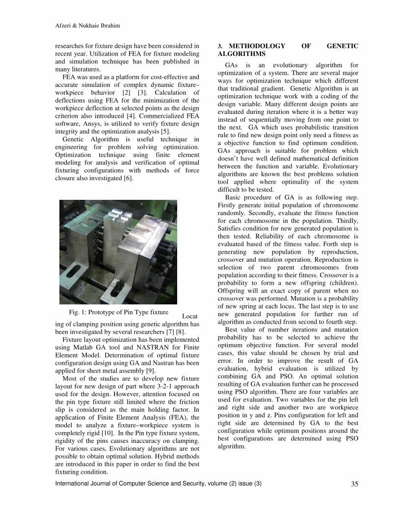
Afzeri & Nukhaie Ibrahim
International Journal of Computer Science and Security, volume (2) issue (3)
35
researches for fixture design have been considered in
recent year. Utilization of FEA for fixture modeling
and simulation technique has been published in
many literatures.
FEA was used as a platform for cost-effective and
accurate simulation of complex dynamic fixture–
workpiece behavior [2] [3]. Calculation of
deflections using FEA for the minimization of the
workpiece deflection at selected points as the design
criterion also introduced [4]. Commercialized FEA
software, Ansys, is utilized to verify fixture design
integrity and the optimization analysis [5].
Genetic Algorithm is useful technique in
engineering for problem solving optimization.
Optimization technique using finite element modeling for analysis and verification of optimal
fixturing configurations with methods of force
closure also investigated [6].
Locat
ing of clamping position using genetic algorithm has
been investigated by several researchers [7] [8].
Fixture layout optimization has been implemented
using Matlab GA tool and NASTRAN for Finite
Element Model. Determination of optimal fixture
configuration design using GA and Nastran has been
applied for sheet metal assembly [9].
Most of the studies are to develop new fixture
layout for new design of part where 3-2-1 approach
used for the design. However, attention focused on
the pin type fixture still limited where the friction
slip is considered as the main holding factor. In
application of Finite Element Analysis (FEA), the
model to analyze a fixture–workpiece system is
completely rigid [10]. In the Pin type fixture system,
rigidity of the pins causes inaccuracy on clamping.
For various cases, Evolutionary algorithms are not
possible to obtain optimal solution. Hybrid methods
are introduced in this paper in order to find the best
fixturing condition.
3. METHODOLOGY OF GENETIC
ALGORITHMS
GAs is an evolutionary algorithm for
optimization of a system. There are several major
ways for optimization technique which different
that traditional gradient. Genetic Algorithm is an
optimization technique work with a coding of the
design variable. Many different design points are
evaluated during iteration where it is a better way
instead of sequentially moving from one point to
the next. GA which uses probabilistic transition
rule to find new design point only need a fitness as
a objective function to find optimum condition.
GAs approach is suitable for problem which
doesn’t have well defined mathematical definition
between the function and variable. Evolutionary
algorithms are known the best problems solution
tool applied where optimality of the system
difficult to be tested.
Basic procedure of GA is as following step.
Firstly generate initial population of chromosome
randomly. Secondly, evaluate the fitness function
for each chromosome in the population. Thirdly, Satisfies condition for new generated population is
then tested. Reliability of each chromosome is
evaluated based of the fitness value. Forth step is
generating new population by reproduction,
crossover and mutation operation. Reproduction is
selection of two parent chromosomes from
population according to their fitness. Crossover is a
probability to form a new offspring (children).
Offspring will an exact copy of parent when no
crossover was performed. Mutation is a probability
of new spring at each locus. The last step is to use
new generated population for further run of
algorithm as conducted from second to fourth step.
Best value of number iterations and mutation
probability has to be selected to achieve the
optimum objective function. For several model
cases, this value should be chosen by trial and
error. In order to improve the result of GA
evaluation, hybrid evaluation is utilized by
combining GA and PSO. An optimal solution
resulting of GA evaluation further can be processed
using PSO algorithm. There are four variables are
used for evaluation. Two variables for the pin left
and right side and another two are workpiece
position in y and z. Pins configuration for left and
right side are determined by GA to the best
configuration while optimum positions around the best configurations are determined using PSO
algorithm.
Fig. 1: Prototype of Pin Type fixture
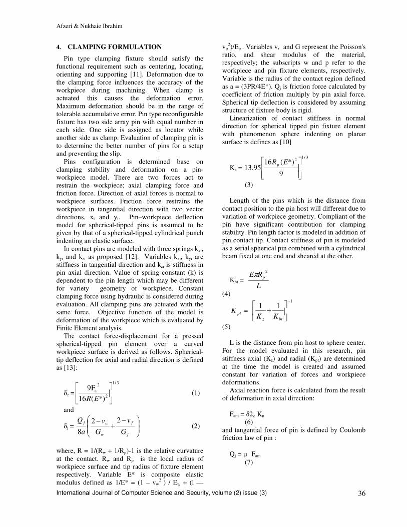
Afzeri & Nukhaie Ibrahim
International Journal of Computer Science and Security, volume (2) issue (3)
36
4. CLAMPING FORMULATION
Pin type clamping fixture should satisfy the
functional requirement such as centering, locating,
orienting and supporting [11]. Deformation due to
the clamping force influences the accuracy of the
workpiece during machining. When clamp is
actuated this causes the deformation error.
Maximum deformation should be in the range of
tolerable accumulative error. Pin type reconfigurable
fixture has two side array pin with equal number in
each side. One side is assigned as locator while
another side as clamp. Evaluation of clamping pin is
to determine the better number of pins for a setup
and preventing the slip.
Pins configuration is determined base on
clamping stability and deformation on a pin-
workpiece model. There are two forces act to
restrain the workpiece; axial clamping force and
friction force. Direction of axial forces is normal to
workpiece surfaces. Friction force restrains the
workpiece in tangential direction with two vector
directions, xi and yi. Pin–workpiece deflection
model for spherical-tipped pins is assumed to be given by that of a spherical-tipped cylindrical punch
indenting an elastic surface.
In contact pins are modeled with three springs kxi,
kyi and kzi as proposed [12]. Variables kxi, kyi are
stiffness in tangential direction and kzi is stiffness in
pin axial direction. Value of spring constant (k) is
dependent to the pin length which may be different
for variety geometry of workpiece. Constant
clamping force using hydraulic is considered during
evaluation. All clamping pins are actuated with the
same force. Objective function of the model is
deformation of the workpiece which is evaluated by
Finite Element analysis.
The contact force-displacement for a pressed
spherical-tipped pin element over a curved
workpiece surface is derived as follows. Spherical-
tip deflection for axial and radial direction is defined
as [13]:
δz =
3/1
2
2
a
*)(16
F9
ER (1)
and
δj =
−
+−
f
f
w
wj
G
v
G
v
a
Q 22
8 (2)
where, R = 1/(Rw + 1/Rp)-1 is the relative curvature
at the contact. Rw and Rp is the local radius of
workpiece surface and tip radius of fixture element
respectively. Variable E* is composite elastic
modulus defined as 1/E* = (1 – vw2
) / Ew + (l —
vp2)/Ep . Variables v, and G represent the Poisson's
ratio, and shear modulus of the material,
respectively; the subscripts w and p refer to the
workpiece and pin fixture elements, respectively.
Variable is the radius of the contact region defined
as a = (3PR/4E*). Qj is friction force calculated by
coefficient of friction multiply by pin axial force.
Spherical tip deflection is considered by assuming
structure of fixture body is rigid.
Linearization of contact stiffness in normal
direction for spherical tipped pin fixture element
with phenomenon sphere indenting on planar
surface is defines as [10]
Kz =
3/12
9
*)(1695.13
ERp
(3)
Length of the pins which is the distance from
contact position to the pin host will different due to
variation of workpiece geometry. Compliant of the
pin have significant contribution for clamping
stability. Pin length factor is modeled in addition of
pin contact tip. Contact stiffness of pin is modeled
as a serial spherical pin combined with a cylindrical beam fixed at one end and sheared at the other.
Kbt = L
RE p
2π
(4)
ptK =
1
11−
+
btz KK
(5)
L is the distance from pin host to sphere center.
For the model evaluated in this research, pin
stiffness axial (Kz) and radial (Kpt) are determined
at the time the model is created and assumed
constant for variation of forces and workpiece deformations.
Axial reaction force is calculated from the result
of deformation in axial direction:
Fam = δ2z Kn
(6)
and tangential force of pin is defined by Coulomb friction law of pin :
Qj = µ Fam
(7)

Afzeri & Nukhaie Ibrahim
International Journal of Computer Science and Security, volume (2) issue (3)
37
5. MODEL FOR FREE FORM GEOMETRY
Free form geometry may be designed using
variety of geometrical formulations. A part model
may be created using a surface equation such as B-
Spline or NURBS or combination between Surface
and Features base modeling.
Contact model between pin and workpiece surface
is defined by three vectors; one normal vector and
two tangential vectors. Normal vector is obtained by
interfere operation between pin and workpiece.
Vector is determined by the direction from contact
point and center of pin. Fig.2 shows CAD simulation
to get contact normal vector.
A tangential vector represents the spring model for restrain the workpiece from slip. First vector is
defined as the vector parallel to x axis of world
coordinate system. Another vector is the cross
product of normal and first tangential vectors.
6. FINITE ELEMENT MODELING
Finite element analysis using Ansys software is
utilized to determine the deformation during
clamping. Workpiece model is imported from
CATIA V5 CAD software and SOLID95 is selected
as material type for meshing. As mentioned in the previous section, three springs are used for a model
of a pin and COMBIN14 is selected as spring model.
Real constants of the spring will be varying for every
pin respect to workpiece geometry. Value of Real
constants is pin stiffness for axial and tangential
direction. Slip is evaluated by comparing pin radial
deflection and workpiece node radial deformation.
Workpiece geometry is modeled using Catia
software and imported to Ansys and meshed using
VSEL command. For PSO Evaluation, the selected
area where the pins are contacted is further refined
using “NREFINE” command. Pin is located to the
node which is closest to actual pin position.
Obtaining the closet not is performed using NODE(
PUX(J),PUY(J),PUZ(J)) command. PUX,PUY and
PUZ are actual pin coordinate while J is pin index.
Following script is codes for refining mesh at pin locations.
!left side pins
*DO,J,1,JPIN/2
*if,CPU(J),EQ,1,THEN
NUPIN = NODE(PUX(J),PUY(J),PUZ(J))
NREFINE,NUPIN, , ,1,1,1,1
*endif
*ENDDO
!right side pins
*DO,J,1,JPIN/2
*if,CPL(J),EQ,1,THEN
NLPIN = NODE(PLX(J),PLY(J),PLZ(J))
NREFINE,NLPIN, , ,1,1,1,1
*endif
*ENDDO
Fig. 3 shows a spring orientation for clamped
workpiece. Support for upper side has three springs
while lower side by two vectors. One another
vector for lower side is hydraulic clamping with
direction always parallel to pin axial axis.
Fig. 2 : Solid Interfere evaluation to obtain
Contact and surface normal
Fig.3 : Pin-Workpiece Contact model

Afzeri & Nukhaie Ibrahim
International Journal of Computer Science and Security, volume (2) issue (3)
38
7. HYBRID EVALUATION USING PSO
ALGORITHM
Genetic algorithms have no mechanisms for
identification absolutely the best solution of
particular problem. However, a solution is "better"
only in comparison to other, presently known
solutions. Algorithm to obtain an optimal solution
has to be tested with another way to check whether a
solution is optimal. Hybrid technique is second
optimization step that runs after the genetic
algorithm terminates in order to improve the value of
the fitness function. The hybrid function uses the
final point from the genetic algorithm as its initial
point. A hybrid function can be specified to improve
the result.
In order to obtain better clamping position, hybrid
evaluation is utilized by combining GAs with PSO
algorithm. The PSO algorithm is utilized to
determine the best position of the workpiece by
shifting around y and z position. Particle Swarm
Optimization (PSO) is a population based stochastic
optimization technique inspired by social behavior of
bird flocking or fish schooling. PSO is initialized with a group of random
particles (solutions) and then searches for optima by
updating generations[15]. In every iteration, each
particle is updated by following two "best" values.
After finding the two best values, the particle
updates its velocity and positions with following
equations.
v[] = v[] + c1 * rand() * (pbest[] - present[]) +
c2 * rand() * (gbest[] - present[]) (7)
present[] = present[] + v[] (8)
v[] is the particle velocity, present[] is the current
particle (solution). pbest[] and gbest[] are defined as
stated before. rand () is a random number.
There are two variables are used for evaluation
using PSO algorithm. Two variables for the pin left
and right side was used for GAs and another two
variables, that are workpiece position in y and z is
utilized for PSO evaluation. Pins configuration for
left and right side it has been determined by GA to
obtain the best configuration is further evaluated
using PSO algorithm to obtain optimum positions of
workpiece around the best configurations.
In order to reduce the time of calculation, larger
mesh size is selected for GAs evaluation and refined
mesh at clamping pin position is performed for PSO.
The best position from range between -5.0 to 5.0 in y
and z position is searched. Amount of movement is
determined by PSO rules. Pins position and contact
vectors are recalculated for new location of
workpiece. Calculation is performed by sending a
message to CAD software using Dynamic Data
Exchange (DDE) interface function.
Twenty numbers of iterations and ten population
sizes has been used with 0.9 initial inertia weight
and 0.4 for final inertia weight.
Fig. 4 shows the overall procedure of
optimization process with sequence explained as
follows. New free form geometry is modeled using
a CAD software. Initial configuration is assigned
through a random number. Number is then
converted to a binary value represent pin
configuration. Clamping model for FEA process is
generated respect to pin configuration model.
Configuration model is evaluated using FEA
software to obtain fitness value. Fitness value is then evaluated by GA rule for next generation of
configuration with iteration process. Finally PSO is
used for fine tuning the result obtained form GAs
evaluation.
Calculate Fitness value
FEAClamping Model
Chromosome
(GAs)
Evaluate Fitness Value
(GAs)
Iteration achieved?
PSO
No
Assign new chromosome
Optimum Configuration
New Free form workiece
Fig. 4 : Hybrid evaluation scenario

Afzeri & Nukhaie Ibrahim
International Journal of Computer Science and Security, volume (2) issue (3)
39
8. CASE STUDY
A prismatic 3D part model is used with geometry
as shown in Fig. 5 and material properties as listed in
Table 2. Cutting force is applied using three forces
in x, y and z directions. There are eight pins in each
side is applied to the model. Result of FEA
computation written using *GET and *VWRITE
command is further evaluated using functions created and executed inside Matlab for finding
optimum clamping configuration using GAs and
PSO. The material properties of the workpiece and
pin elements are given in Table 1.
Table 1 Table Material Properties used for FEA
Workpiece Pin
element
Material Alloy Steel Tool
Steel
Young’s modulus (GPa) 206 217
Shear modulus (GPa) 73 73
Poisson’s ratio 0.3 0.3
Static friction coefficient 0.35
The evaluation source codes are created using
Matlab and interfaced with Ansys for calculation the objective function. First process is assigning initial
parameters such as number of iteration, population
size and generating meshed workpiece model with
no supporting and clamping pin. Meshed workpiece
is used to obtain the node number for contacted pins.
Second process is generating pin workpiece model
with configuration as defined by chromosome codes.
Spring constant for used pins in radial (Kr) and axial
(Ka) are calculated and the result is stored in pin-
workpiece model data. The next process is
evaluation the clamping model using FEA to obtain
maximum deformation and deformation at pin
contacted nodes. Deformation data is used to
calculate friction slip and fitness value. Slip in pin
contacted nodes is occurring when workpiece
tangential deformation is more that pin deformation
due to friction force. Configuration is categorized
as violation if slip in any contacted pin is observed.
The evaluation process is repeated until reach the
assigned number of populations and generations.
Optimum configuration obtained from GAs
evaluation is then evaluated using PSO to obtain
minimum workpiece deformation by shifting the
workpiece position. PSO will search the optimum position with the configuration obtained by GAs.
Workpiece location in x and z direction are
dimension parameters adjusted during iteration
processes of PSO evaluation. Random number is
generated in the range of pin distance in x and z
direction.
The magnitude of 500N clamping force is used for every pin. Cutting force is applied at right
surface. Parameter uses during GAs evaluation is
listed in Table 2.
Table 2. GAs Parameters
Parameter Value
Population Size Generations
Migration Fraction
Crossover Function
Mutation Function
10 20
0.39796
1.1316
0.2907
Result of GAs evaluation with complete iteration
is given in Fig. 6. Optimum configuration after 20
generations is 0.0591 with pin configuration
chromosome 0000001100101110 and
0000111011001100 for left and right side
respectively. Actual pin configuration converting
Fig. 5: Sample workpiece evaluated using
FEA for final clamp configuration
Fig. 6: Result of Genetic Algorithm for 20
generations

Afzeri & Nukhaie Ibrahim
International Journal of Computer Science and Security, volume (2) issue (3)
40
from the chromosome code is shown in the Fig. 5
which have 6 pins for supporting and 7 pins as
clamping.
The hybrid function uses the final point
from the genetic algorithm as its initial point. A
hybrid algorithm is used to improve the result.
The second algorithms using PSO are performed
to determine the best position of the workpiece.
The area between -5.0 to 5.0 in y and z position
is searched by dynamically move the workpiece.
Value 5.0 mm is the half distance between two
closest pins. Process of iteration using PSO rule
is shown in Fig. 7. Result after evaluation was
shift the workpiece position by 1.3950 and -
0.7576 in y and z direction respectively with
fitness 0.0541. PSO optimization was moving
the workpiece to new location with the less
amount of clamping deformation.
9. CONCLUSION
Spherical type pin fixture has been considered as
suitable tools to hold a free from workpiece
geometry. Evaluation of clamping ability has been
performed through Finite Element Analysis for
computation of workpiece deformation and detection
of slip. Three springs for representing a pin contact
vectors possible to reduce the calculation time
during iteration process.
Optimization of pin configuration and position for
pin type fixture was enabling to minimize workpiece
deformation during clamping. The simulation model
developed using Genetic Algorithms and PSO
algorithms integrated with Finite element method
enable to obtain the better configuration of pin
respect to minimum deformation.
Optimization technique was performed using
hybrid algorithms, GAs and PSO, with four input
parameters. Result of optimization process enables
to obtain the better pin configurations and clamping
positions.
ACKNOWLEDGEMENT
This research is supported by a grand from FRGS
2007 with contract number FRGS 0106-2.
REFERENCES
[1] Afzeri, A.G.E. Sutjipto, A.K..M Nurul Amin,
Riza Muhida, 2005, Pin type reconfigurable
Clamping ability evaluation for Setup-Free
Technology, ICOMMS, Kuala Lumpur.
[2] J.H. Yeh, F.W. Liou, 1999,Contact condition
modelling for machining fixture setup processes, Int. J. Mach. Tools Manuf. 39
787–803.
[3] R.O. Mittal, P.H. Cohen, B.J. Gilmore, 1991,
Dynamic modelling of the fixture–workpiece
system, Robot. Comput.-Integr. Manuf. 8 (4)
204–217.
[4] R.J. Menassa, W.R. DeVries, 1991,
Optimization methods applied to selecting
support positions in fixture design, ASME
Journal of Engineering for Industry 113 412–
418.
[5] N. Amaral, J.J. Rencis, Y. Rong, 2004,
Development of a finite element analysis tool
for fixture design integrity verification and
optimisation, International Journal of
Advanced Manufacturing Technology 21
411–419.
[6] E.Y.T. Tan, A.S. Kumar, J.Y.H. Fuh, A.Y.C.
Nee, 2004, Modeling, analysis and
verification of optimal fixturing design, IEEE
Transactions on Automation Science and
Engineering 1 (2) 121–132.
[7] Necmettin, K., 2006, Machining fixture
locating and clamping position optimization
using genetic algorithms, Computers in Industry 57 112–120.
[8] A.S. Kumar, V. Subramaniam, K.C. Seow,
1999, Conceptual design of fixtures using
genetic algorithms, International Journal of Advanced Manufacturing Technology 15, pp
79–84.
Fig. 7: Dynamics of workpiece Positions during
PSO evaluation.

Afzeri & Nukhaie Ibrahim
International Journal of Computer Science and Security, volume (2) issue (3)
41
[9] Y.G. Liao, 2003, A genetic algorithm-based
fixture locating positions and clamping
schemes optimization, Proceedings of the
Institute of Mechanical Engineers. Part B,
Journal of Engineering Manufacture 217, pp
1075–1083.
[10] Shane P. Siebenaler, Shreyes N. Melkote, 2006,
Prediction of workpiece deformation in a
fixture system using the finite element method,
International Journal of Machine Tools &
Manufacture 4651–58.
[11] A.Y.C. Nee, K. Whybrew, A. Senthil Kumar,
1995, Advanced Fixture Design for FMS,
Springer, London.
[12] Haiyan Deng, Shreyes N. Melkote, 2006,
Determination of minimum clamping forces for
dynamically stable fixturing ,International
Journal of Machine Tools & Manufacture 46,
847–857
[13] Anand Raghu, Shreyes N. Melkote, 2004,
Analysis of the effects of fixture clamping
sequence on part location errors, International
Journal of Machine Tools & Manufacture 44
373–382
[14] Ibrahim M. Deiab, Mohamed A. Elbestawi, 2005, Experimental determination of the
friction coefficient on the workpiece-fixture
contact surface in work holding applications
International Journal of Machine Tools &
Manufacture 45 705–712.
[15] http://www.swarmintelligence.org/tutorials.ph
p
[16] Afzeri, A.G. E. Sutjipto, A.K.M. Nurul Amin,
Riza Muhida, 2005, Determination of pin
configuration for clamping fixture by means
of solid model contact analysis, Proceedings
of the International Conference on Mechanical
Engineering (ICME), Dhaka, Bangladesh.
NOMENCLATURE
c1 First learning factors of PSO algorithm.
c2 Second learning factors of PSO algorithm.
δz spherical clamping static deformation at axial
direction
δj spherical clamping static deformation at radial
direction
δ2r
pin static deformation at radial direction
δ2j
pin static deformation at tangential direction
E elastic modulus
Fa axial reaction force at jth pin
G Shear modulus
v Poisson’s ratio
Kz
pin stiffness at axial direction
Kbt radial stiffness of cantilever bream fixed at one
end
Kpt spherical pin stiffness for tangential direction
L Pin length, distant from host to contact surface
P clamping force
Q tangential contact forces of pin.
R Pin radius
µ Static friction coefficient