edges, orientation, hog and sift - university of...

Edges, Orientation, HOG and SIFT

D.A. Forsyth

Linear Filters

• Example: smoothing by averaging• form the average of pixels in a neighbourhood

• Example: smoothing with a Gaussian• form a weighted average of pixels in a neighbourhood

• Example: finding a derivative• form a weighted average of pixels in a neighbourhood

Smoothing by Averaging

Nij =1N

�uvOi+u,j+v

where u, v, is a window of N pixels in total centered at 0, 0

• A Gaussian gives a good model of a fuzzy blob

Smoothing with a Gaussian

• Notice “ringing” • apparently, a grid is

superimposed

• Smoothing with an average actually doesn’t compare at all well with a defocussed lens• what does a point of light

produce?

Gaussian filter kernel

Kuv =⇤

12�⇥2

⌅exp

⇧�

�u2 + v2

⇥

2⇥2

⌃

We’re assuming the index can take negative values

Smoothing with a Gaussian

Nij =�

uv

Oi�u,j�vKuv Notice the curious looking form

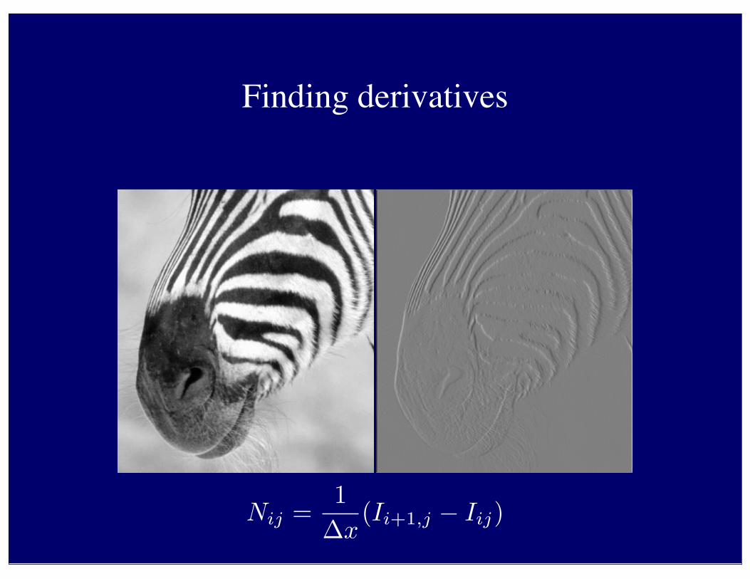
Finding derivatives

Nij =1

�x(Ii+1,j � Iij)

• Each of these involves a weighted sum of image pixels• The set of weights is the same • we represent these weights as an image, H• H is usually called the kernel

• Operation is called convolution• it’s associative

• Any linear shift-invariant operation can be represented by convolution• linear: G(k f)=k G(f)• shift invariant: G(Shift(f))=Shift(G(f))• Examples: • smoothing, differentiation, camera with a reasonable, defocussed lens

system

Convolution

Nij =�

uv

HuvOi�u,j�v

Filters are templates

• At one point• output of convolution is a (strange) dot-product

• Filtering the image involves a dot product at each point• Insight • filters look like the effects they are intended to find• filters find effects they look like

Nij =�

uv

HuvOi�u,j�v

Normalised correlation

• Think of filters of a dot product• now measure the angle• i.e normalised correlation output is filter output, divided by root sum of

squares of values over which filter lies• Tricks:• ensure that filter has a zero response to a constant region • helps reduce response to irrelevant background

• subtract image average when computing the normalising constant• absolute value deals with contrast reversal

normalised correlationwith non-zero mean filter

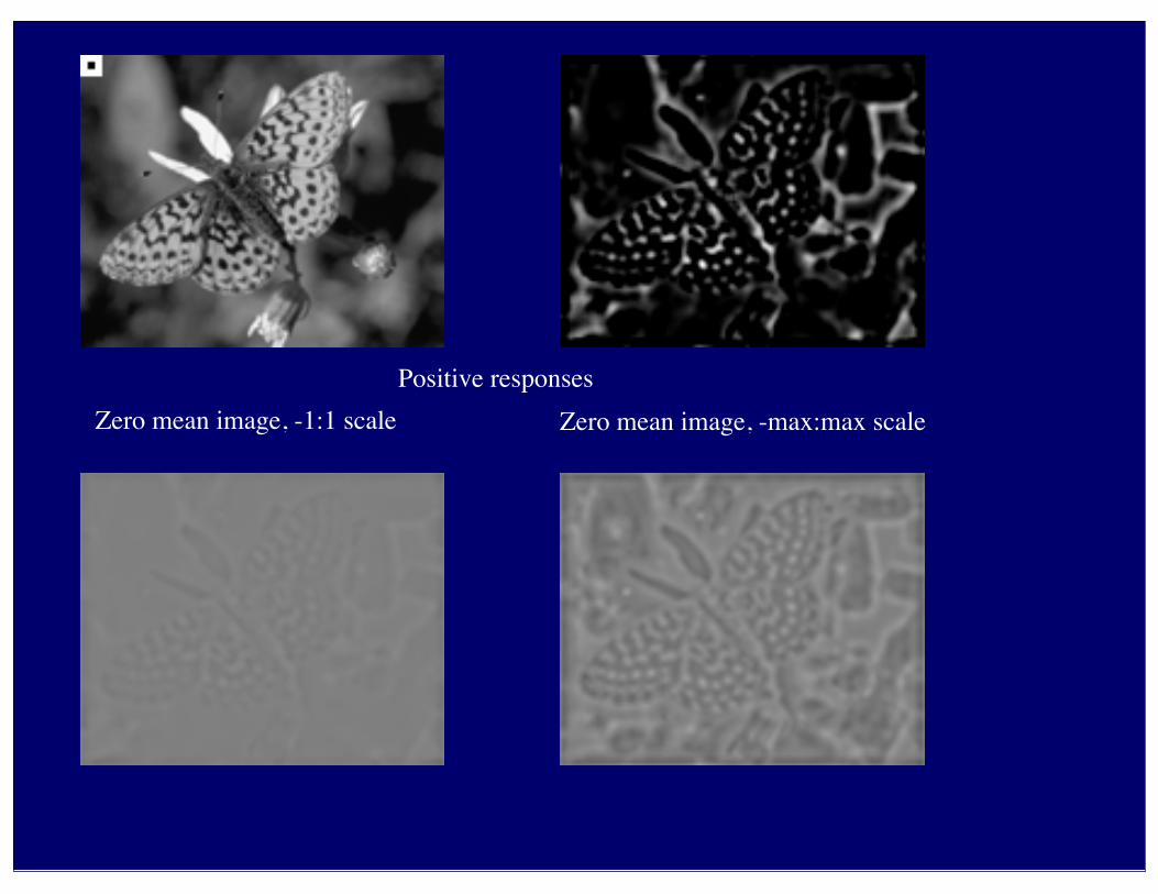
Positive responsesZero mean image, -1:1 scale Zero mean image, -max:max scale

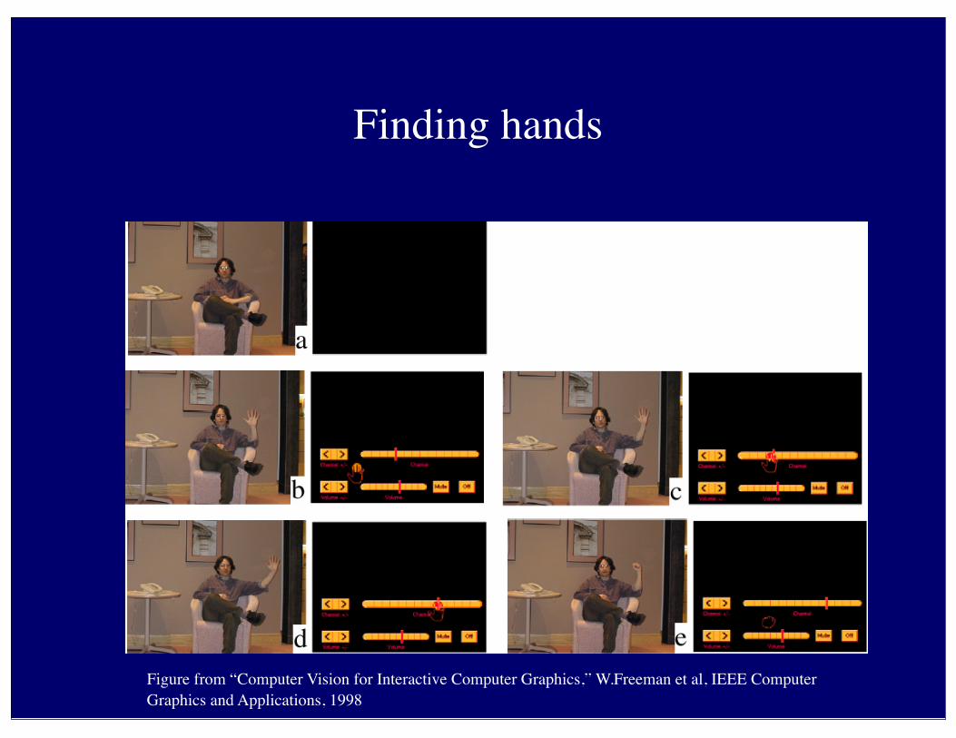
Finding hands

Figure from “Computer Vision for Interactive Computer Graphics,” W.Freeman et al, IEEE Computer Graphics and Applications, 1998

Noise

• Simplest noise model• independent stationary additive Gaussian noise• the noise value at each pixel is given by an independent draw from the

same normal probability distribution

• Issues• allows values greater than maximum camera output or less than zero• for small standard deviations, this isn’t too much of a problem

• independence may not be justified (e.g. damage to lens)• may not be stationary (e.g. thermal gradients in the ccd)

sigma=1

sigma=4

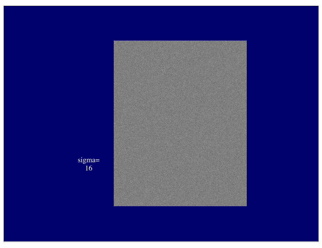
sigma=16

sigma=1

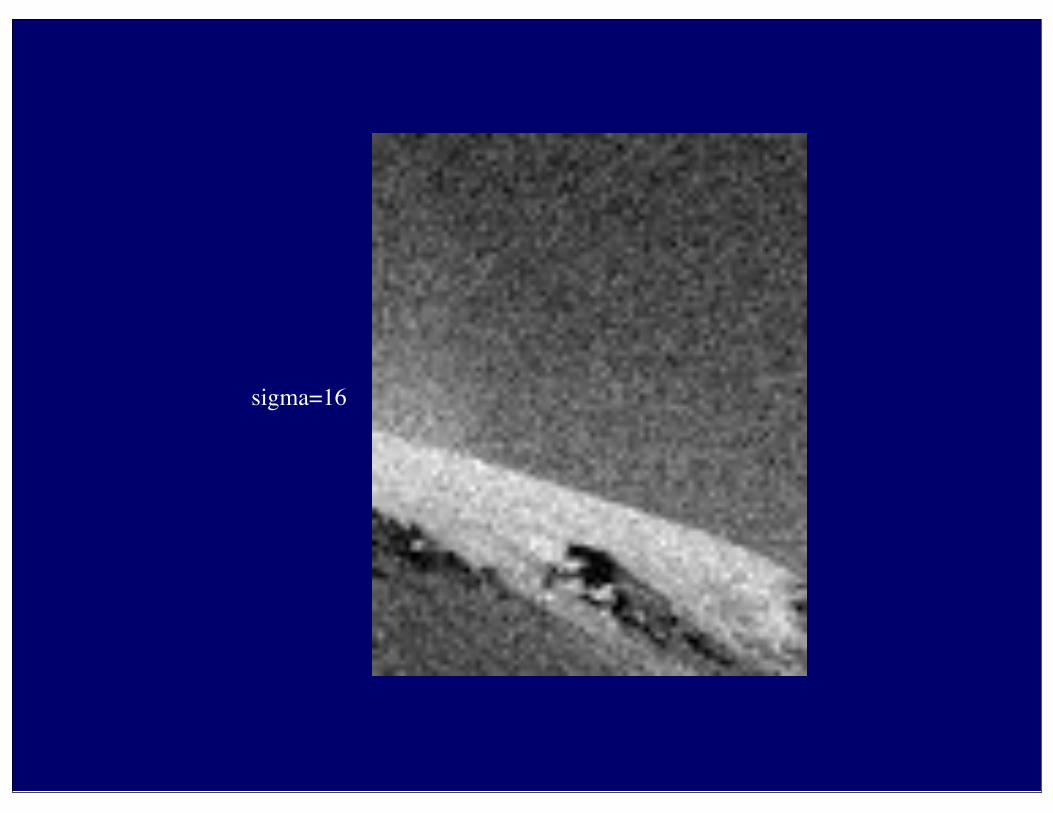
sigma=16

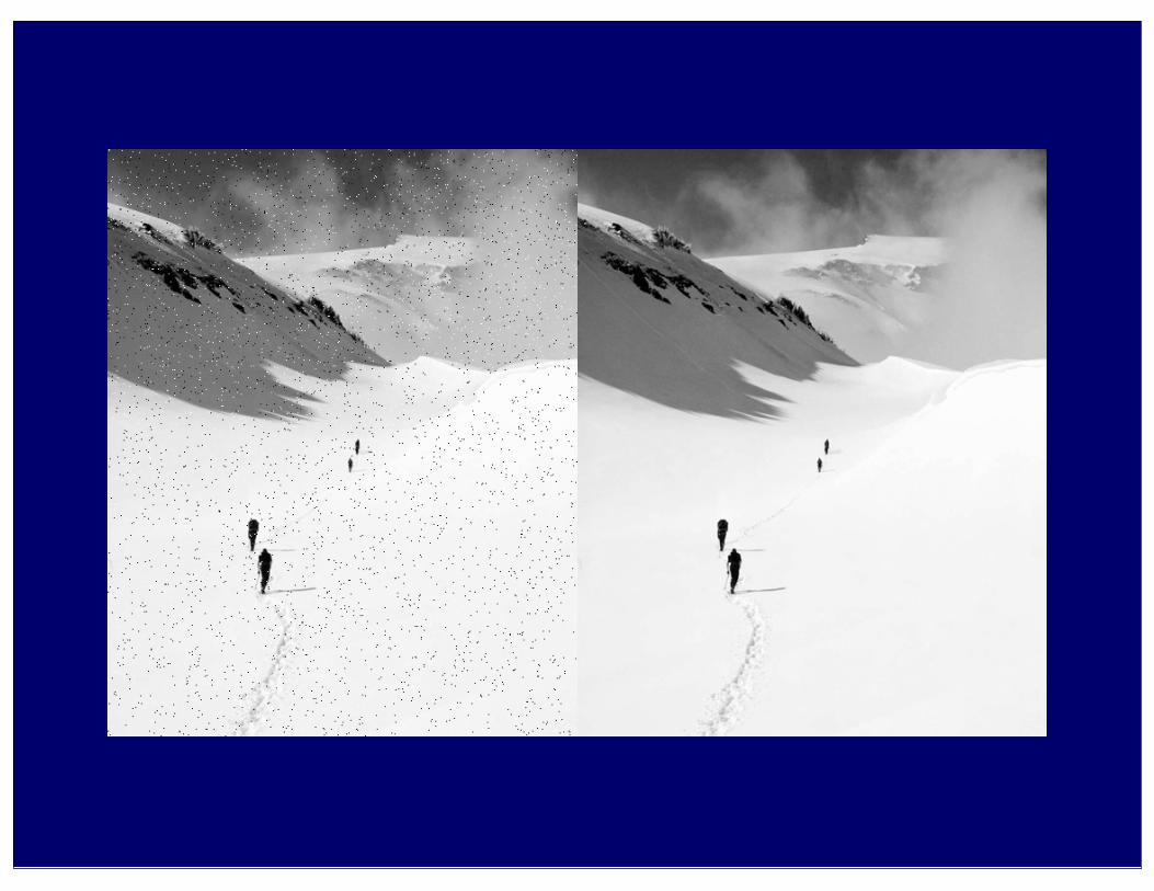
Smoothing reduces noise

• Generally expect pixels to “be like” their neighbours• surfaces turn slowly• relatively few reflectance changes

• Expect noise to be independent from pixel to pixel• Implies that smoothing suppresses noise, for appropriate noise models

• Scale• the parameter in the symmetric Gaussian• as this parameter goes up, more pixels are involved in the average• and the image gets more blurred• and noise is more effectively suppressed

Kuv =⇤

12�⇥2

⌅exp

⇧�

�u2 + v2

⇥

2⇥2

⌃

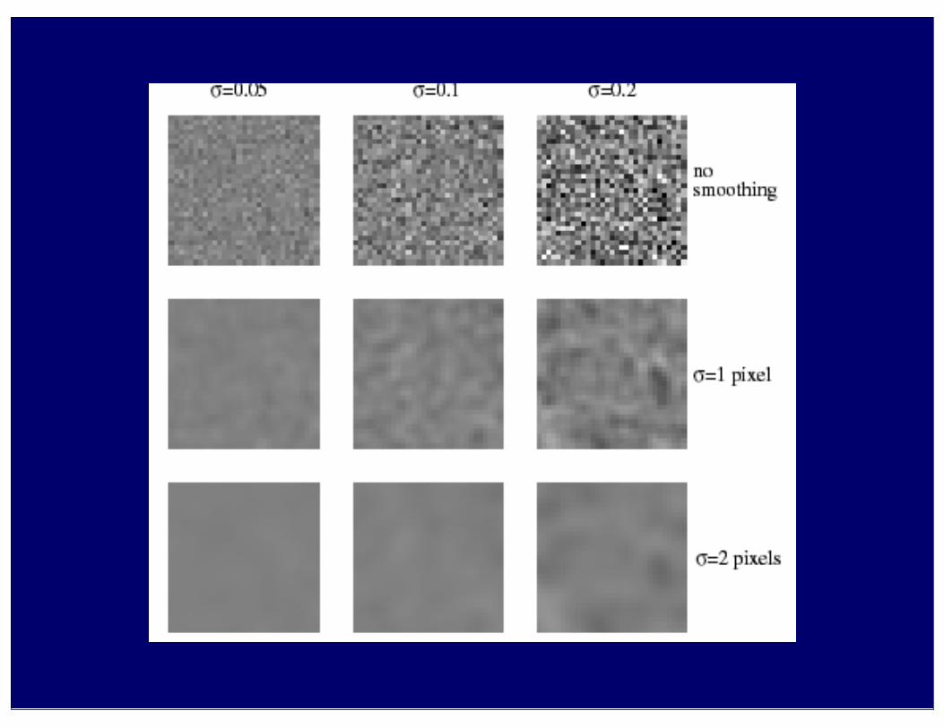
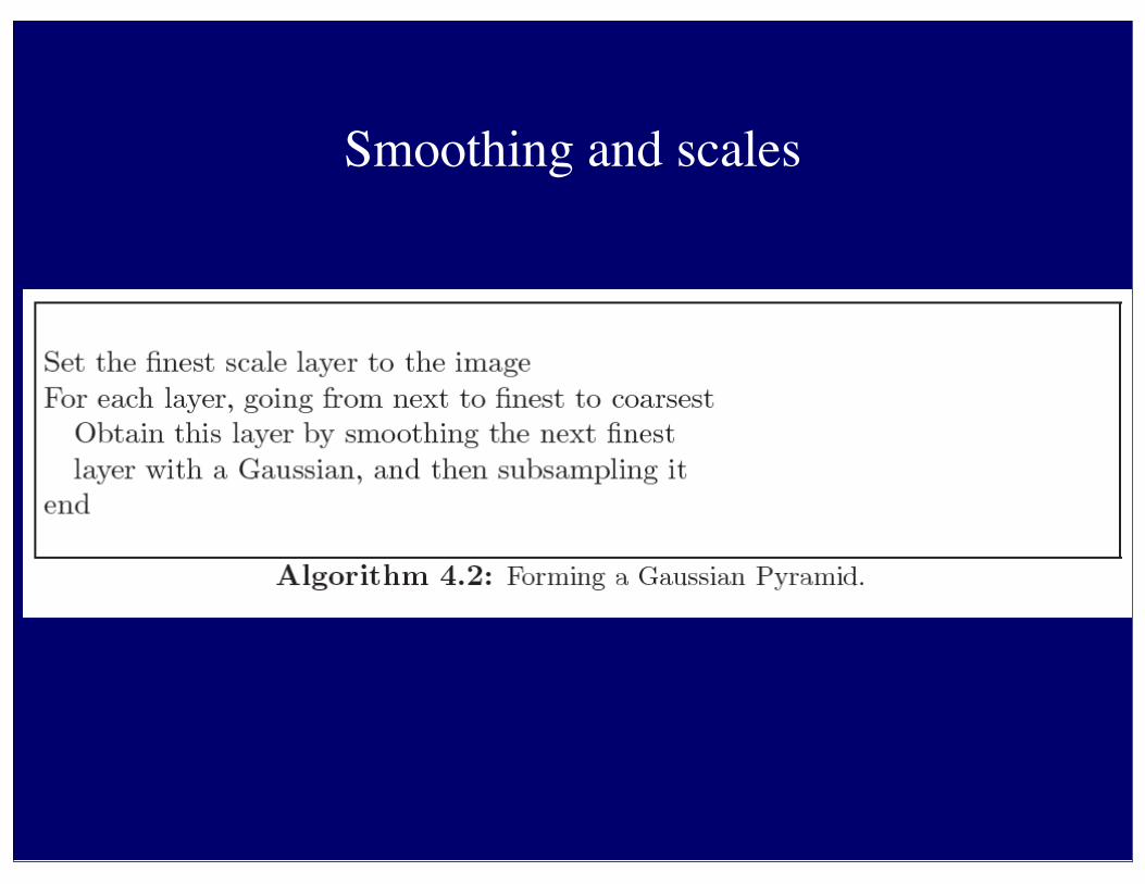
Smoothing and scales

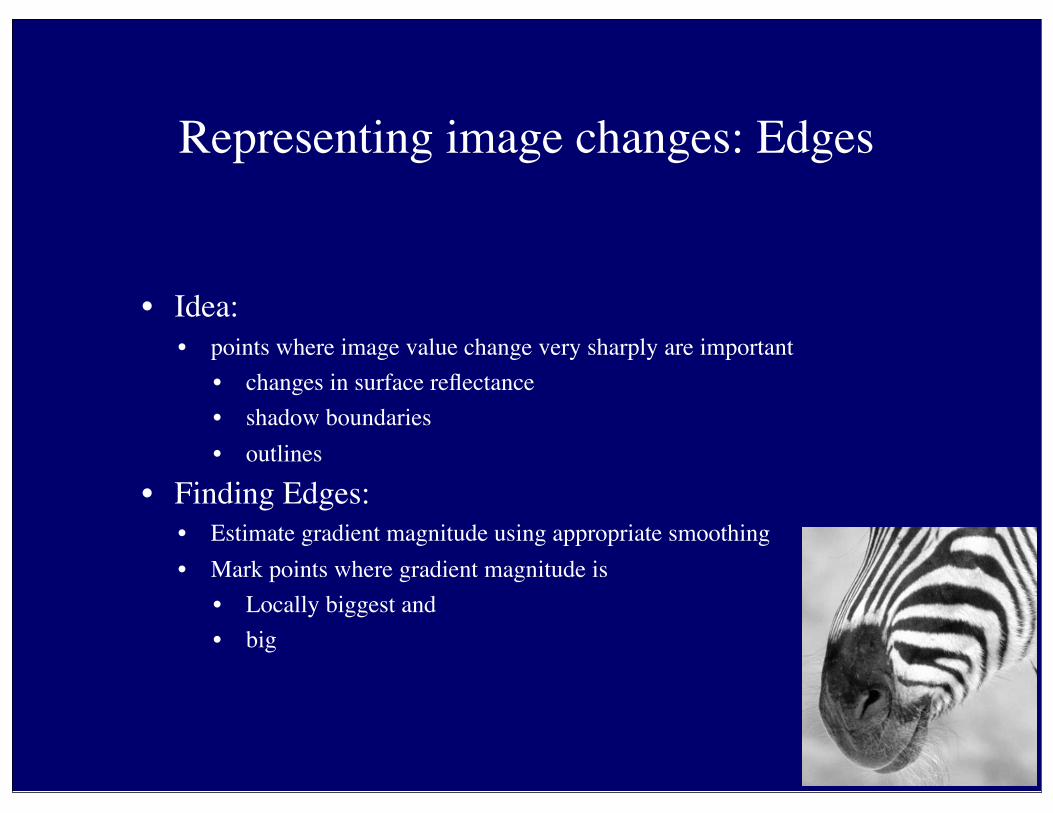
Representing image changes: Edges

• Idea:• points where image value change very sharply are important

• changes in surface reflectance• shadow boundaries• outlines

• Finding Edges:• Estimate gradient magnitude using appropriate smoothing• Mark points where gradient magnitude is

• Locally biggest and• big

Smoothing and Differentiation

• Issue: noise• smooth before differentiation• two convolutions to smooth, then differentiate?• actually, no - we can use a derivative of Gaussian filter

1 pixel 3 pixels 7 pixels

Scale affects derivatives

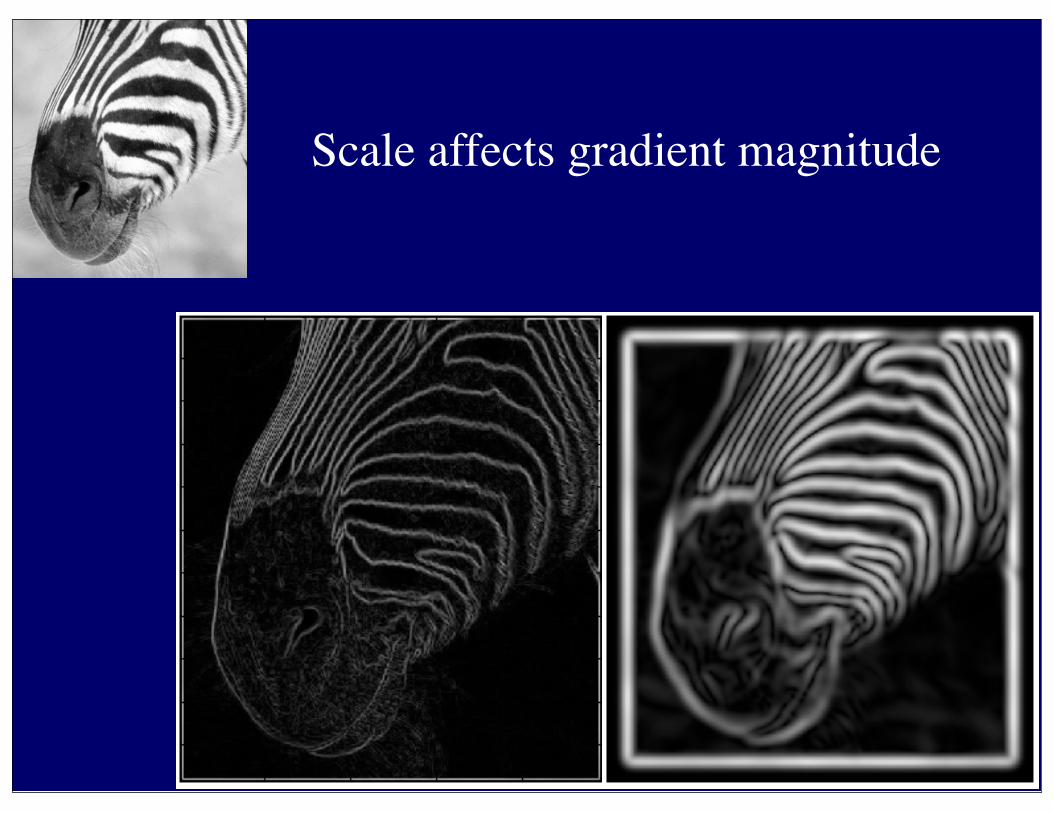
Scale affects gradient magnitude

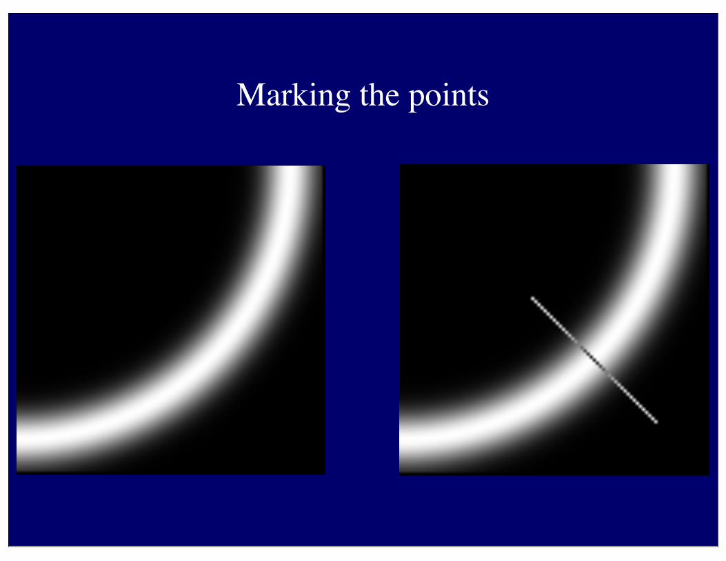
Marking the points

Non-maximum suppression

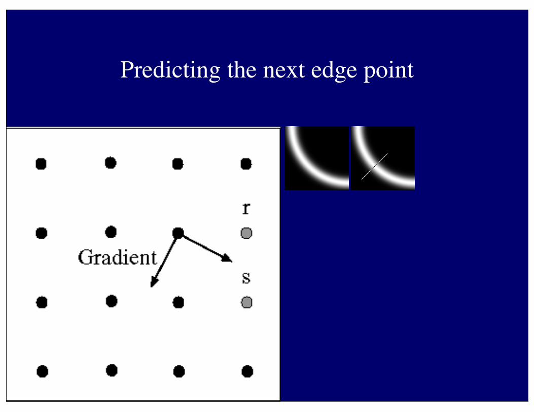
Predicting the next edge point

Remaining issues

• Check maximum value of gradient value is sufficiently large• drop-outs?

• use hysteresis

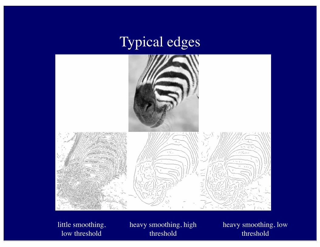
Typical edges

little smoothing, low threshold

heavy smoothing, high threshold

heavy smoothing, low threshold

Notice

• Something nasty is happening at corners• Scale affects contrast• Edges aren’t bounding contours

The Laplacian of Gaussian

• Another way to detect an extremal first derivative is to look for a zero second derivative

• Appropriate 2D analogy is rotation invariant• Laplacian

• Edges are zero crossings• Bad idea to apply a Laplacian without smoothing• smooth with Gaussian, apply Laplacian• this is the same as filtering with a Laplacian of Gaussian filter• Now mark the zero points where • there is a sufficiently large derivative, • and enough contrast

The Laplacian of Gaussian

Filters and Edges: Crucial points

• Filters are simple detectors• they look like patterns they find

• Smoothing suppresses noise• because pixels tend to agree

• Sharp changes are interesting• because pixels tend to agree• easy to find - edges

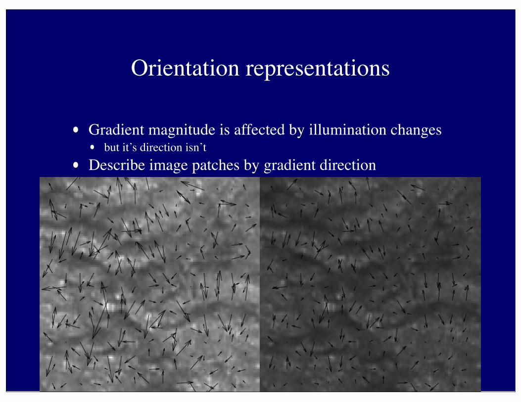
Orientation representations

• Gradient magnitude is affected by illumination changes• but it’s direction isn’t

• Describe image patches by gradient direction

Orientations

Orientations at different scales

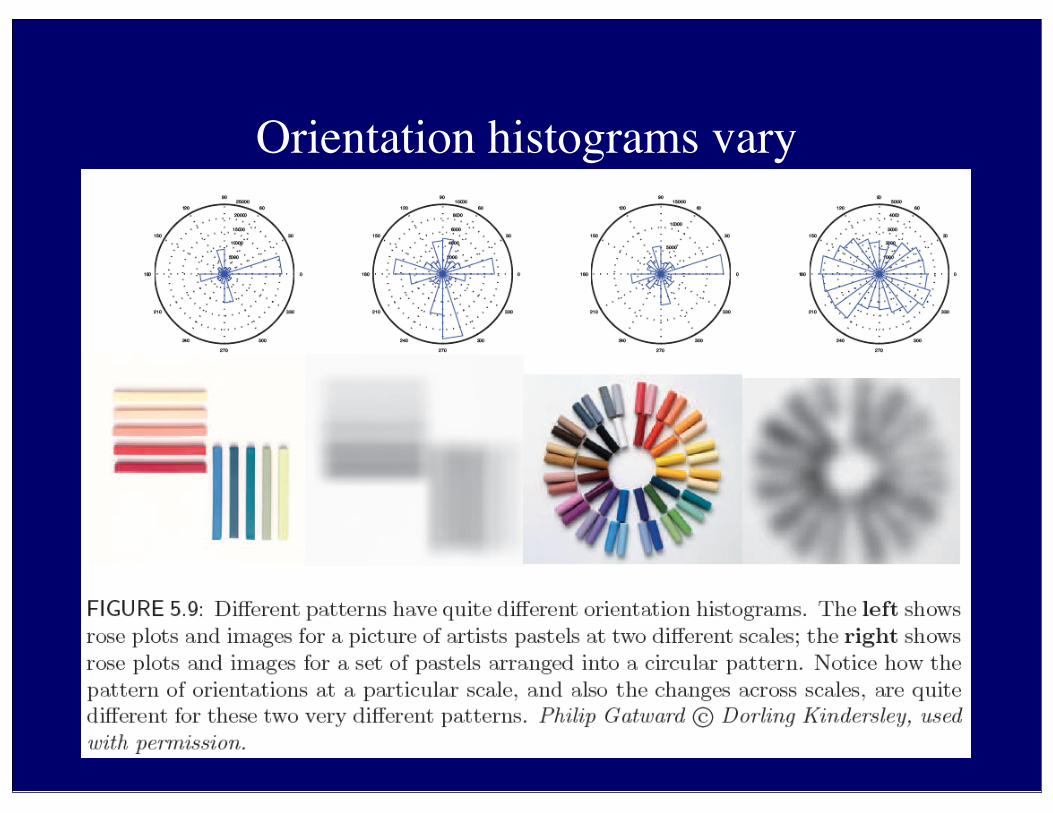
Orientation histograms vary

Histograms of oriented gradients

• Strategy:• break patch up into blocks• construct histogram representing gradients in that block• which won’t change much if the patch moves slightly

• Variants• histogram of angles• histogram of gradient vectors, length normalized by block averages

HOG features

Histograms of oriented gradients

From Deva Ramanan’s lake Como slides

HOG features

Interest points

• Automatic patch construction• HOG works if we know the patch • but what patches should we use?• sliding windows

• We then• find patches• make descriptions• match patches

• Matches for• making mosaics• spotting near duplicates• detection• reconstruction

K. Grauman, B. Leibe

B1

B2

B3A1

A2 A3

Interest points

• For image, find center/radius of circles “worth describing”• these should be “stable”• if the image is panned, the centers should pan• if the image is scaled, the centers should scale

Interest points: locating centers

• We use a corner detector (Harris, 88)• at a corner there are• strong gradients• in different directions

• Use second moments of derivatives


32

1. Image derivatives

2. Square of derivatives

3. Gaussian filter g(σI)

Ix Iy

Ix2 Iy2 IxIy

g(Ix2) g(Iy2)g(IxIy)

har

g(IxIy)

Interest points: finding the radius


Laplacian of Gaussian: radius or blob detector

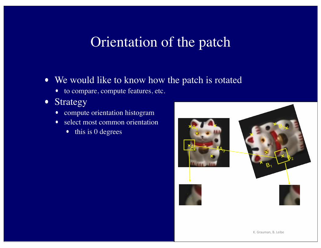
Orientation of the patch

• We would like to know how the patch is rotated• to compare, compute features, etc.

• Strategy• compute orientation histogram• select most common orientation• this is 0 degrees


B1

B2

B3A1

A2 A3

Describing patches

• Various histograms of orientation• HOG• SIFT• SURF• etc.

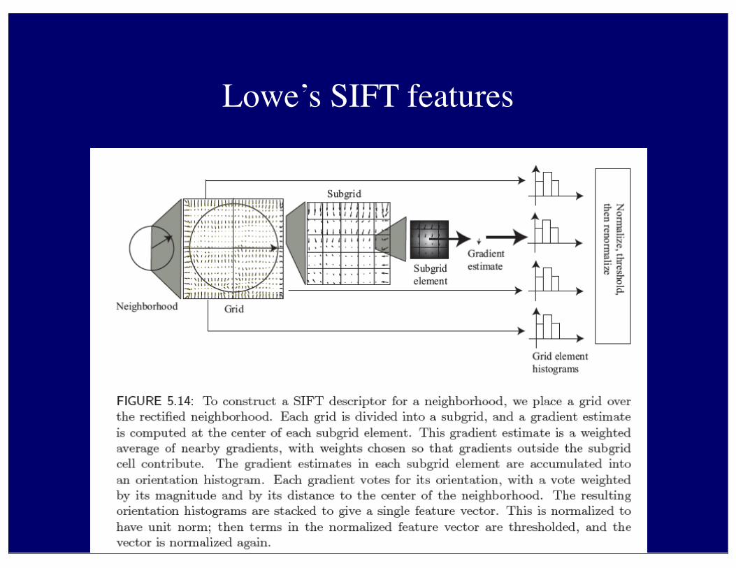
Lowe’s SIFT features

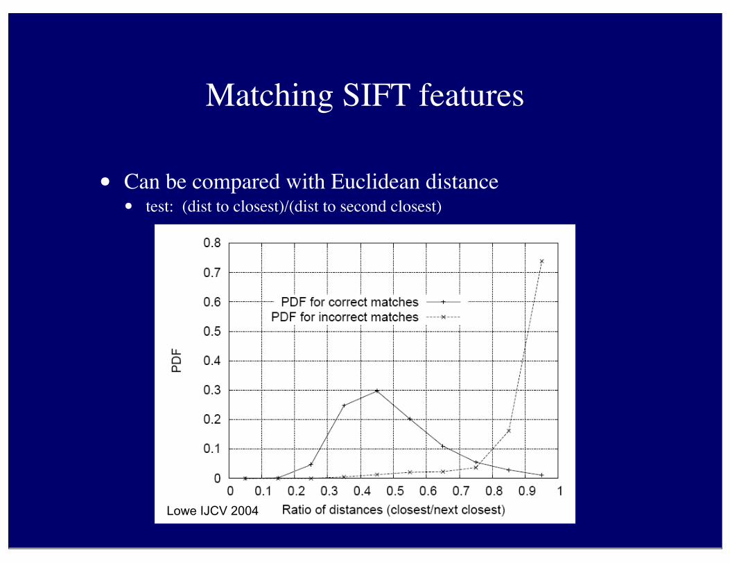
Matching SIFT features

• Can be compared with Euclidean distance• test: (dist to closest)/(dist to second closest)

Lowe IJCV 2004

HOG and SIFT - Crucial points

• Orientation based descriptors are very powerful• because robust to changes in brightness

• HOG feature• known window, make histogram of orientations

• SIFT feature• find domain

• patch center and radius• compute descriptor

• histogram of orientations

• Numerous powerful variants• Software available

Software, etc

edges, orientation, hog and sift - university of...

Documents