CS201: Computer Vision Lect 09: SIFT Descriptors

John Magee 26 September 2014

Slides Courtesy of Diane H. Theriault

Questions of the Day:

• How can we find matching points in images?

• How can we use matching points to recognize objects?

SIFT

• Find repeatable, scale-invariant points in images (Tuesday)

• Compute something about them (Today)

• Use the thing you computed to perform matching (Today)

• A lot of engineering decisions

• “Distinctive Image Features from Scale-Invariant Keypoints” by David Lowe

• Patented!

How to find the same cat?

• Imagine that we had a library of cats

• How could we find another picture of the same cat in the library?

• Look for the markings?

Scale Space

• Image convolved with Gaussians of different widths

Keypoints with Image Filtering

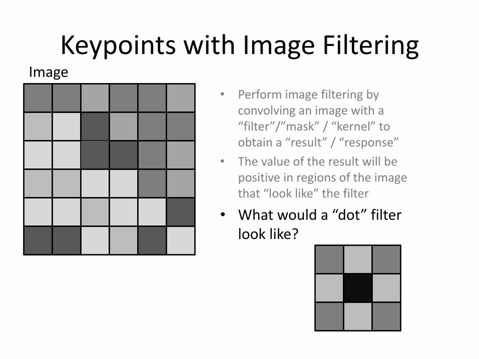
• Perform image filtering by convolving an image with a “filter”/”mask” / “kernel” to obtain a “result” / “response”

• The value of the result will be positive in regions of the image that “look like” the filter

• What would a “dot” filter look like?

Image

Filter

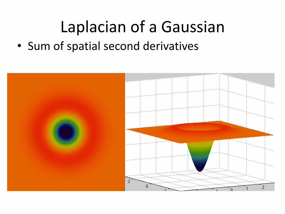
Laplacian of a Gaussian • Sum of spatial second derivatives

Difference of Gaussians

• Approximation of the Laplacian of a Gaussian

Scale-space Extrema

• “Extremum” = local minimum or maximum

• Check 8 neighbors at a particular scale

• Check neighbors at scales above and below

Scale-space Extrema • Find locations and scales where the response to

the LoG filter is a local extremum

Removing Low Contrast Points

• Threshold on the magnitude of the response to the LoG filter

• Threshold empirically determined

Removing Points Along Edges

• In 1D: first derivative shows how the function is changing (velocity)

• In 1D: second derivative how the change is changing (acceleration)

• In 2D: first derivative leads to a gradient vector, which has a magnitude and direction

• In 2D: second derivatives lead to a matrix, which gives information about the rate and orientation of the change in the gradient

Removing Points Along Edges

• Hessian is a matrix of 2nd derivatives

• Eigenvectors tell you the orientation of the curvature

• Eigenvalues tell you the magnitude

• Ratio of eigenvalues tells you extent to which one orientation is dominant

Gradient of a Gaussian

Hessian of a Gaussian

Attributes of a Keypoint

• Position (x,y)

– location in the image

• Scale

– scale where this point is a LoG extremum

• Orientation?

Gradient Orientation Histogram

• Make a histogram over gradient orientation

• Weighted by gradient magnitude

• Weighted by distance to key point

• Contribution to bins with linear interpolation

Gradient Orientation Histogram

Gradient orientation histogram

Gradient Orientation Histogram

• Plain Histogram of Gradient Orientation

Gradient Orientation Histogram

• Weighted by gradient magnitude

• (Could also weight by distance to center of window)

Gradient Orientation Histogram

• Interpolated to avoid edge effects of bin quantization

Assigning Orientation to Keypoint

• Support: from image at assigned scale, all points in a window surrounding keypoint

• 36 bins over 360 degrees

• Contributions weighted by distance to center of key point, weighted by a Gaussian with sigma 1.5 x assigned scale

Dominant orientation

Computing SIFT Descriptor

• Divide 16 x 16 region surrounding keypoint into 4 x 4 windows

• For each window, compute a histogram with 8 bins

• 128 total elements

• Interpolation to improve stability (over orientation and over distance to boundary of window)

Computing SIFT Descriptor

• Divide 16 x 16 region surrounding keypoint into 4 x 4 windows

• For each window, compute a histogram with 8 bins

• 128 total elements

• Interpolation to improve stability (over orientation and over distance to boundary of window)

Normalizing the descriptor

• To get (some) invariance to brightness and contrast

– Clamp weight due to gradient magnitude (In case some edges are very strong due to weird lighting)

– Normalize entire vector to unit length (So the absolute value of the gradient magnitude isn’t as important as the distribution of the gradient magnitude)

Using the keypoints

• Assemble a database:

– Pick some “training” images of different objects

– Find keypoints and compute descriptors

– Store the descriptors and associated source image, position, scale, and orientation

Using the keypoints

• New Image

– Find keypoints and compute descriptors

– Search database for matching descriptors

– (Throw out descriptors that are not distinctive)

– Look for clusters of matching descriptors

• (e.g. In your new image, you found 10 keypoints and associated descriptors, and in the database, there is an image where 6 of the descriptors match, but only 1 or 2 on other database images)

Using the keypoints

– http://chrisjmccormick.wordpress.com/2013/01/24/opencv-sift-tutorial/

Voting for Pose

• Matching keypoints from database image and new image will imply some relationship in pose (position, scale, and orientation)

– Example: This keypoint was found 20 pixels down and 50 pixels to the right of the matching descriptor from the database image

– Example: This keypoint was computed at 2x the scale of the matching descriptor from the database image

– Look for clusters of matches with similar offsets

– (“Generalized Hough Transform”)

Discussion Questions

• What types of invariance do we want to have when we think about doing object recognition?

• What does it mean to be invariant to different image attributes? (brightness, contrast, position, scale, orientation)

• What does it mean for an image feature to be stable?

• Why might it make sense to use a weighted histogram? What kinds of weights?

• What is a problem with the quantization associated with creating a histogram and what can we do about it?