Economies of Scope and Patterns of Outsourcing

Zhihao Yu*Carleton University

Abstract

The paper suggests that the evolution of modern technologies in manufacturing, from economies-of-scale to economies-of-scope, plays a key role in the increasing outsourcing activities. It isshown that the divergence in the degrees of economies-of-scope and the attribute space of theproducts between different stages of production is the fundamental economic force behind therecent trend of outsourcing activities. It also finds that outsourcing occurs in the following twoopposite scenarios: either (i) the degree of economies-of-scope is very high and the attributespace is very small (i.e., close to a homogenous good); or (ii) the degree of economies-of-scope isvery low and the attribute space is very large (i.e. highly specialized input/service). Further-more, technology progress that reduces market transaction costs always increases outsourcing;technology progress that improves production techniques, however, could either increase or de-crease outsourcing.

JEL Classification No.: L22, F2Key Words: Address Model/Spatial Competition, economies-of-scope, Outsourcing

–––––––—*Department of Economics, Carleton University; Research Fellow of the Leverhulme Centre for Research

on Globalization and Economic Policy (GEP) at the University of Nottingham. I wish to thank Nicolas

Schmitt and John Sutton for valuable comments. Thanks are also extended to the participants at the

Annual Meeting of the Academy of International Business, the Far East Meeting of the Econometric

Society, the Royal Economic Society annual meeting, and the Conference on “New Dimensions in Inter-

national Trade” at Kobe University, seminar at Wilfrid Laurier University. The usual disclaimer applies.

Financial support from the Social Sciences and Humanities Research Council of Canada is gratefully

acknowledged.

Correspondence: Department of Economics, Carleton University, 1125 Colonel By Drive, Ottawa, Ont.

K1S 5B6, Canada; Tel: 1-613-520-2600 ext. 3763; Fax: 1-613-520-3906; Email: zhihao.yu@gmail.com or

zhihao yu@carleton.ca

1 Introduction

Outsourcing is surging in popularity across a wide range of production activities and sectors.

In the automobile industry, for instance, we see outsourcing ranging from product design, data

processing, assembly, special components, and minor parts and components, etc. This raises

a number of critical questions. Why do modern manufacturing firms engage in very different

kinds of outsourcing business in that some require high-skilled labor and are very specialized

but others are very simple and minor? What kind of intermediate input/service do firms often

choose for outsourcing? Can we say anything about the characteristics/attributes of the goods

or services in outsourcing? More importantly, what is the fundamental economic force behind

the recent trend of outsourcing? In this paper we attempt to answer these questions and better

understand the patterns of outsourcing.

Outsourcing is often viewed as a means for firms to cope with increasing competition by

looking for cheaper suppliers. However, while cost reduction is a motive, it is not the underlying

economic force behind outsourcing activities. This paper develops a simple model of two-stage

production in which the evolution of modern production technology (from economies-of-scale

to economies-of-scope) play a key role in outsourcing. The model allows us to discuss how

outsourcing activities are affected by the degree of product differentiation and economies-of-

scope in production of the intermediate input relative to that of the final good.

There are have been two major evolutions in modern manufacturing. The first was the arrival

of economies-of-scale production technology, which requires a large fixed cost in production.

The key to the success of the economies-of-scale technology is to produce a massive amount of

products to achieve low average costs of production. For example, the Ford Motor Company

was a perfect example of succeeding in economies-of-scale production in the automobile industry.

Its relatively inexpensive automobiles was based on mass production of a single, and basically

unchanging, product. In the 1920s when workers in the Ford Motor Company were getting the

highest pay in the industry, Ford did not seek outsourcing to reduce costs,1 nor did the technical

improvements/progresses in economies-of-scale technology lead to outsourcing.

The second major evolution in modern manufacturing was the arrival of economies-of-scope

1Henry Ford introduced the famous ‘five-dollar day’, which doubled the sums he was paying his workforce at a time when the American economy was beginning to lurch into a deep recession (Raff, 1991).

1

production technology. In the automobile industry, for example, in the early 1920s the General

Motors Company started a major innovation in producing automobiles by focusing on economies-

of-scope, rather than economies-of-scale, in production. In 1923 General Motors introduced the

policy of ‘a car for every purse’ (i.e., different cars for people with different incomes) and started

annual model changes. To make model changes relatively cheap, GM had to install multi-

purpose machines and design more common parts into the cars of various models. GM even

published its specification lists of some parts and components, thereby enabling other carmakers

to share in any upstream economies. These changes ultimately lead to outsourcing business in

the General Motors company and the automobile industry.

GM’s innovation of focusing on economies-of-scope was further advanced by Japanese car-

makers (i.e. Toyota and Nissan) after the Second World War. To accommodate consumer

preferences for product variety in the changing world, in contrast to Ford’s vertically-integrated

production system, Toyota built a flexible manufacturing system relying heavily on subsidiaries

and other suppliers. This had a profound impact on the increasing outsourcing activities in

Japanese automobile industry. According to Edward Davis (1992), typically the degree of out-

sourcing is 60-70 percent in Toyota compared to 30-40 percent in General Motors. The success

of economies-of-scope production was also fueled by the progress in the CAD (computer-aided-

design) technology, which has made model changes and product improvement much easier than

ever before.

The evolution of modern manufacturing was one of the main subjects of research interests

in the industrial organization literature over a decade ago. Important contributions in the

literature include Milgrom and Roberts (1990), and Milgrom, Qian and Roberts (1991). These

studies show that firms could exercise flexibility in a number of dimensions, including inventory

policy, product market strategy, the internal organization of the firm, and the number and at-

tributes of products. The focus of these studies is on flexible manufacturing, complementarities

in production, and the theory of firm organization, rather than the outsourcing phenomenon.2

Outsourcing has become the most significant industrial phenomenon since the 1990s and has

widely spread across national boundaries.3 This has generated increasing research interest in

2The implication of flexible manufacturing for market structure has been investigated extensively byMacLeod, et al (1988), Eaton and Schmitt (1994), and Norman and Thisse (1999).

3See evidence of international outsourcing in Hanson (1996), Slaughter (1995), and Feenstra andHanson (2003), among many others. Feenstra (1998) provides an excellent overview of this topic.

2

pursuing rigorous theories for outsourcing. Most studies in the literature use the approaches

based on the theories of incomplete contracts and transaction costs, and focused on the impact

of globalization on outsourcing.4

In this paper we use an address model of spatial competition and focus on the impact

of evolutions of modern manufacturing (i.e. from economies-of-scale to economies-of-scope) on

outsourcing. The spatial model allows us to gain new insights on the patterns of outsourcing and,

in particular, on how outsourcing activities are affected by the degrees of product differentiation

and economies-of-scope in production of the intermediate input relative to those of the final

good. In addition, the address helps better understand the fundamental economic force behind

outsourcing.

The main results of the paper are as follows. First, we show that economies-of-scope in

production is the necessary condition for outsourcing. Adoption of economies-of-scope tech-

nology in production could lead to outsourcing. Second, outsourcing occurs in the following

two opposite scenarios in terms of production and characteristics of the good: either (i) the

degree of economies-of-scope is very high and the attribute space is very small (i.e., close to a

homogenous good), or (ii) the degree of economies-of-scope is very low and the attribute space

is very large (i.e., highly specialized input/service). Third, although economies-of-scope is a

necessary condition for outsourcing, the fundamental economic force behind outsourcing is the

divergence in the degrees of economies-of-scope, and the attribute spaces of the products between

different stages of production. Forth, the progress of the ‘general-purpose-technology’ (e.g., in-

formation technology, etc.) that reduces market transaction costs always increases outsourcing.

However, if technology progress improves production techniques, it could either increase or de-

crease outsourcing activities. Finally, if technology progress is what we called ‘pro-EOScope’

(or ‘anti-EOScope’) and is persistently biased towards one stage of production, outsourcing will

eventually occur.

The rest of the paper is organized as follows. Section 2 develops a model in which economies-

of-scope play a key role in different stages of production in a vertically-linked production struc-

ture. We then examine both the vertically-integrated and vertically-disintegrated production

structures, and derive the production-efficiency outcome. Section 3 characterizes the patterns of

4E.g. see McLaren (2000), Grossman and Helpman (2002, 2005), Antras (2003), and Antras andHelpman (2004).

3

outsourcing and discusses the impact of technology progresses on outsourcing activities. Section

4 discusses some alternative assumptions and the robustness of our results. Section 5 concludes

the paper.

2 The Model

There are two goods in the economy, a differentiated product and a numeraire good. Following

the standard circular model for differentiated product, we assume that each good is described

by a point x in some continuum of product attributes represented by a circumference of a circle

of length L. Each consumer is assumed to purchase only one unit of the differentiated good

at price p(x) and has a quasi-linear preference. The indirect utility function for consumer i is

given by

Vi = v − t|x− xoi |+ I − p(x) (1)

where xoi describes consumer i’s most preferred differentiated good (or the consumer’s address

in the attribute space), v is the consumer’s reservation price, and t is the marginal disutility

of distance in the attribute space. Assume that v is large so that in equilibrium all individuals

consume the differentiated good. Income I comes from wages only and is identical for each

consumer. There are L consumers, whose preference of attributes for the most preferred good

is uniformly distributed along a circumference.

2.1 Vertically-Integrated (In-house) Production

Suppose labor is the only primary input factor in the economy. The numeraire good is produced

by a constant-return-to-scale technology using labor only and, by choice of units, it uses one

unit of labor to produce one unit of output. This implies that the wage rate is equal to one,

and therefore I also represents the constant labor supply of each individual.

To produce the differentiated product, it requires a two-stage production structure, in which

the technology of both production stages exhibits economies-of-scope. In addition to the

direct labor input, to produce one unit of final output requires one unit of an intermediate

input/component,5 which is also produced using labor. Specifically, in both stages of produc-

tion, firms must first incur a fixed cost to develop a basic product and then they can produce

5For the sake of clarity, we assume only one intermediate input/component. The model can be easilygeneralized to use many intermediate components to produce the final good and our results will remain.

4

variants by modifying the basic product. We use Xi to denote the location in the final-good

attribute space of basic product i, and xj that of variant j; Similarly, we use Yi and yj for that

of the intermediate good, respectively. This simple two-stage production structure is illustrated

in Figure 1.

Assume that each firm owns at most only one basic product in each stage of production.6

Therefore a firm is identified by a basic product. Suppose that qi(xj) is the quantity of variant

j (j = 1, ...,m) produced from basic product i (including the basic product — a ‘variant’ with

no modification from Xi). The overall production can be described by

(x,qi) = [(x1, qi(x1)], [x2,qi(x2)], ..., [(xm, qi(xm)] (2)

We assume that the overall production cost takes the following form,

C((x,qi);Xi) = K+mXj=1

qi(xj)(ecyi + cx + rx|xj −Xi|) (3)

= K +C((y,qi);Yi)+mXj=1

qi(xj)(cx + rx|xj −Xi|), K > 0, rx > 0

where ecyi is the average cost and C((y,qi);Yi) the total cost of the variants of the basic inter-mediate input Yi. Specifically,

ecyi = C((y,qi);Yi)/ mXj=1

qi(xj), j = 1, ...,m (4)

C((y,qi);Yi) = k+mXj=1

qi (xj) (cy + ry|yj − Yi|), k > 0, ry > 0 (5)

Parameters K and k respectively denote the fixed costs of developing the basic final and inter-

mediate product (Xi and Yi). The term cy + ry|yj − Yi| is the marginal cost of producing oneunit of variant yj, where ry|yj − Yi| is the incremental marginal cost of modification. Similarly,ecyi +cx+rx|xj−Xi| is the marginal cost of producing one unit of variant xj using input yj . Thefurther away a variant (xj or yj) is from its basic product, the larger the cost of modification.

Parameters rx and ry are (constant) unit modification costs (i.e., per unit of the attribute space).

Without loss of generality, for the rest of our analysis we assume cx = cy = 0.

6Even if firms can own more than one basic product at each stage of production, our results remain aslong as there are additional organizational costs of having more than one basic product at each stage ofproduction. This is similar to the common assumption in the literature that there are cost advantagesfor specialized firms. In Section 4 we relax this assumption.

5

Following the standard definition7, the degree of economies-of-scope in the final-good pro-

duction can be characterized by

(m− 1)K − rxPmj=1 qi(xj)|xj −Xi|

C((x,qi);Xi)> 0 (6)

The trade-off is between saving the fixed costs and incurring the modification costs. For

economies-of-scope to exist, either K has to be large or rx has to be small so that (6) is positive.

The higher the degree of economies-of-scope, the larger the value of K and/or the smaller the

value of rx. Similarly, the degree of economies-of-scope in the intermediate-good production is

given by(m− 1)k − ryPm

j=1 qi(xj)|yj − Yi|C((y,qi);Yi)

> 0 (7)

Therefore, K and rx (resp. k and ry) are the key parameters that determine the degree of

economies-of-scope in production of the final (resp. intermediate) good.

2.1.1 Equilibrium with economies-of-scale

When production only has economies-of-scale but not economies-of-scope, a firm produces only

the basic product. Then, (3) and (5) reduce to:

C(Xi) = K + qiecyi and C(Yi) = k (8)

where qi is output (of the basic product), and ecyi = cyi ≡ C(Yi)/qyi since there are no variantsproduced except for the basic product. In this case, minimum-cost production requires that

the basic intermediate product Yi is designed to fit exactly the production of Xi

Suppose there are n firms symmetrically located along the circumference of a circle in the

attribute space. In the symmetric equilibrium under free entry, we obtain the following results

(e.g. Tirole, 1988):

pi = L/no + cyi and cyi =

kno

L, i = 1, ..., n (9)

7As in Pepall, et al (1999), for example, the degree of economies of scope is defined by

C(Q1, 0) +C(0, Q2)−C(Q1, Q2)C(Q1, Q2)

where C(., .)s represent the costs of producing the products independently, or jointly.

6

where

no = L(1/K)1/2 (10)

Therefore, the average cost of production of the intermediate input and the price of the final

good become

cy ≡ cyi = k/(K)1/2, i = 1, ..., n (11)

p ≡ pi = K1/2 + k/(K)1/2, i = 1, ..., n (12)

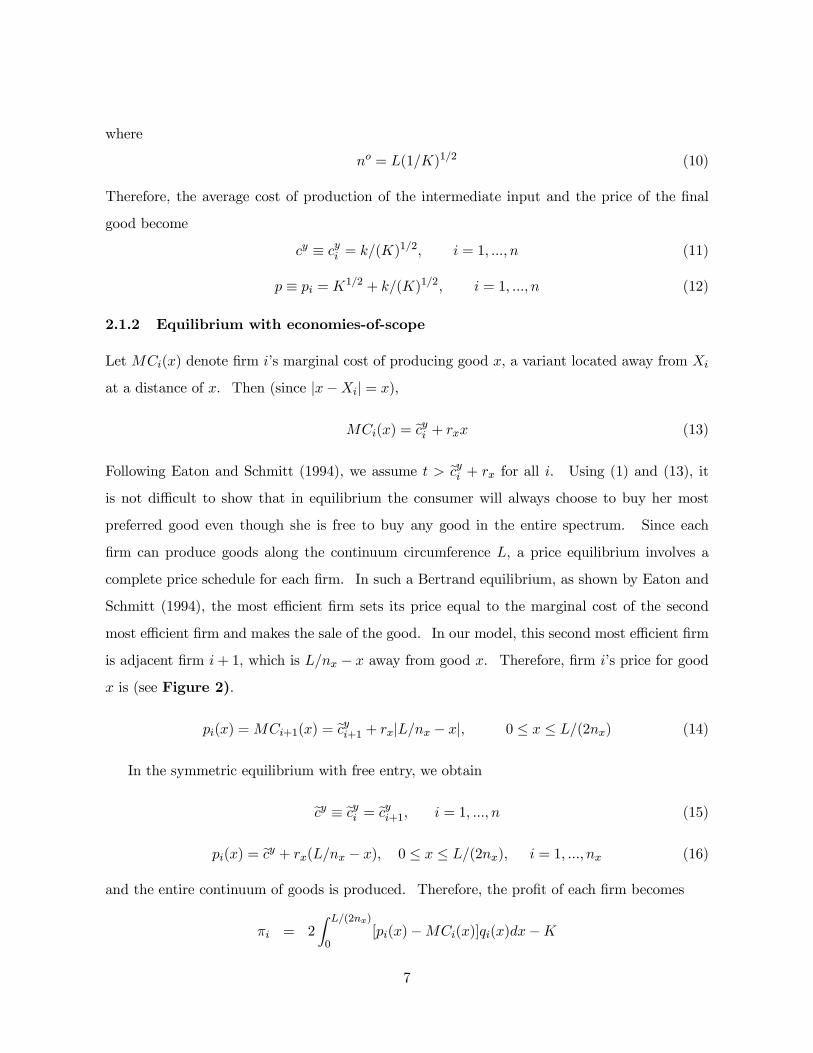
2.1.2 Equilibrium with economies-of-scope

Let MCi(x) denote firm i’s marginal cost of producing good x, a variant located away from Xi

at a distance of x. Then (since |x−Xi| = x),

MCi(x) = ecyi + rxx (13)

Following Eaton and Schmitt (1994), we assume t > ecyi + rx for all i. Using (1) and (13), it

is not difficult to show that in equilibrium the consumer will always choose to buy her most

preferred good even though she is free to buy any good in the entire spectrum. Since each

firm can produce goods along the continuum circumference L, a price equilibrium involves a

complete price schedule for each firm. In such a Bertrand equilibrium, as shown by Eaton and

Schmitt (1994), the most efficient firm sets its price equal to the marginal cost of the second

most efficient firm and makes the sale of the good. In our model, this second most efficient firm

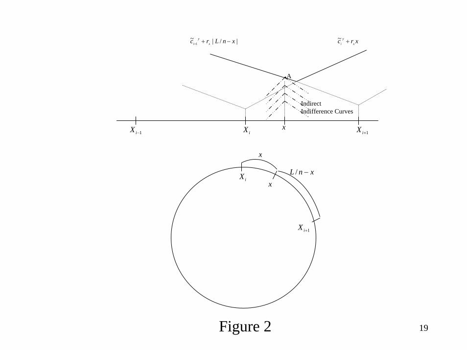
is adjacent firm i+ 1, which is L/nx − x away from good x. Therefore, firm i’s price for good

x is (see Figure 2).

pi(x) =MCi+1(x) = ecyi+1 + rx|L/nx − x|, 0 ≤ x ≤ L/(2nx) (14)

In the symmetric equilibrium with free entry, we obtain

ecy ≡ ecyi = ecyi+1, i = 1, ..., n (15)

pi(x) = ecy + rx(L/nx − x), 0 ≤ x ≤ L/(2nx), i = 1, ..., nx (16)

and the entire continuum of goods is produced. Therefore, the profit of each firm becomes

πi = 2Z L/(2nx)

0[pi(x)−MCi(x)]qi(x)dx−K

7

= 2

Z L/(2nx)

0[rx(L/nx − x)− rxx]dx−K (17)

=rx2(L

nx)2 −K

Free entry will drive πi down to zero. Ignoring the ‘integer issue’, we obtain the equilibrium

number of firms:

nox = L(rx2K

)1/2 (18)

To calculate the average cost of the intermediate good, it is important to notice that, in

general, the distance of |yj − Yi| is not the same as that of |xj −Xi| since the attribute spacefor the final good does not have to be the same as that for the intermediate input. Suppose

that the length of the circumference of the attribute space for the intermediate good is θL, as

illustrated in Figure 1. Then, if θ < 1 (resp. θ > 1), the attribute space of the intermediate

input is smaller (resp. greater) than that of the final good.

Furthermore, notice that ny = nox in vertically-integrated production. Using (4-5), we can

obtain the average cost of the intermediate good:8

ecy ≡ ecyi = k + 2R θL/(2ny)0 qi(y)ryydy

2R θL/(2ny)0 qi(y)dy

=k + 2

R θL/(2nox)0 (ryy/θ)dy

2R θL/(2nox)0 (1/θ)dy

(19)

=k + (θryK)/(2rx)

(2K/rx)1/2

= k(rx2K

)1/2 +θry2(K

2rx)1/2

Using (16) and (18-19), we obtain the equilibrium price of good x:

po(x) ≡ poi (x) = k(rx2K

)1/2 +θry2(K

2rx)1/2 + rx[(

2K

rx)1/2 − x], i = 1, ..., n (20)

where x ∈ [0, (Krx )1/2].

2.2 Vertically-Disintegrated Production (Outsourcing) and the Production-Efficiency Outcome

Now consider the case in which production is vertically-disintegrated, and there are independent

firms and markets for the intermediate input. To avoid any unnecessary strategic action in the

8Notice that for the attribute space of intermediate input y, the length of the circumference becomesθL, and the density 1/θ.

8

intermediate-input market and focus on the fundamental economic force in production (i.e.,

production efficiency), we assume free entry and no cross-subsidizing in the intermediate input

market so that the intermediate products are priced at average costs. Similar to Grossman and

Helpman (2005), we also assume that final-good producers have to incur transaction costs in

purchasing the intermediate input.

2.2.1 Equilibrium with economies-of-scale

When production only has economies-of-scale but not economies-of-scope, only the basic prod-

ucts are produced. Therefore, in equilibrium the number of the basic final-good products has

to equal that of the basic intermediate-input products. Furthermore, minimum-cost production

requires that the basic intermediate product Yi is designed to fit exactly the production of Xi.

Thus, the equilibrium is exactly the same as vertically-integrated production in Section 2.1.1,

except that firms now have to pay transaction costs for the input they purchase. Therefore,

vertically-integrated production will dominate vertically-disintegrated production.

Proposition 1 Without economies-of-scope (i.e., with only economies-of-scale) technology,

vertically-integrated production is more efficient than vertically-disintegrated production.

2.2.2 Equilibrium with economies-of-scope

When there are economies-of-scope in production, the number of the basic intermediate products

no longer has to equal that of the basic final products. Suppose there are ny firms in the

intermediate-input market, and they are located symmetrically along a circumference θL in

attribute space. For a representative firm i, which produces variants located symmetrically

from its basic intermediate input Yi, the total cost of production is

C((y,qyi );Yi) = k + 2

Z θL/(2ny)

0qj(y)ryydy

= k + 2Z θL/(2ny)

0(ryy/θ)dy (21)

= k +θry4(L

ny)2

and the average cost of each variant becomes

cyi =C((y,qyi );Yi)

2R θL/(2ny)0 qj(y)dy

9

=k + (θry/4)(L/ny)

2

2R θL/(2ny)0 (1/θ)dy

(22)

= (kny +θryL

2

4ny)/L

Under free-entry, the average cost of intermediate input will be driven down to the minimum.

Therefore, the equilibrium number of firms in the intermediate-input market is given by

noy = argmin (kny +θryL

2

4ny)/L

= L(θry4k)1/2 (23)

Substituting (23) into (22), we obtain the average cost of the intermediate input in the symmetric

equilibrium,

cy ≡ cyi

= [kL(θry4k)1/2 +

L

2(θkry)

1/2]/L (24)

= (θkry)1/2 i = 1, ..., n

Vertically-disintegrated production, however, requires transaction costs in purchasing the

intermediate input. For simplicity, we assume that to use one unit of the intermediate input,

a final-good producer has to purchase 1 + τ units of the intermediate input (τ > 0, in units of

output). Thus, the cost for using one unit of the intermediate input is cy(1 + τ).

Therefore, comparing cy(1 + τ) with ecy of (19) in Section 2.1.1, we obtain the followingproposition.

Proposition 2 With economies-of-scope technology,

(i) the production-efficient outcome is in-house production if (θKry)/(krx) ∈ [Ω2L(τ),Ω2U (τ )];however,

(ii) the production-efficiency outcome is outsourcing if (θKry)/(krx) < Ω2L(τ), or (θKry)/(krx) >

Ω2U (τ), where Ω2L(τ) ≡ 2(1+ τ)− [(1+ τ)2−1]0.52 and Ω2U (τ) ≡ 2(1+ τ)+ [(1+ τ )2−1]0.52.

Proof: Before comparing ecy with cy(1 + τ), we first derive ecy/cy. Using (19) and (24), weobtain ecy

cy= (

1

2)0.5(

krxKθry

)0.5 + (1

8)0.5(

Kθrykrx

)0.5 (25)

=1

Ω(1

2)0.5 +Ω(

1

8)0.5

10

where Ω ≡ [(θKry)/(krx)]0.5. It is easy to show that (25) reaches the minimum (equal to 1) at

Ω =√2. Now we compare (ecy/cy) in (25) with (1 + τ). It is not difficult to show that ecy >

cy(1 + τ) if (θKry)/(krx) ∈ [Ω2L(τ ),Ω2U (τ)], and ecy < cy(1 + τ) if (θKry)/(krx) < Ω2L(τ), or

(θKry)/(krx) > Ω2U (τ ).

Proposition 2 is also illustrated in Figure 3. When (θKry)/(krx) ∈ [Ω2L(τ),Ω2U (τ)],

(ecy/cy)-curve is below (1 + τ)-line and we have the ‘In-house Production’ region. When

(θKry)/(krx) < Ω2L(τ) or (θKry)/(krx) > Ω

2U (τ), (ecy/cy)-curve is above (1 + τ)-line and we

have the ‘Outsourcing’ region.

The intuitions for the results are as follows. First, notice that with vertically-disintegrated

production (i.e. outsourcing), the number of basic intermediate products noy in (23) is production-

efficient; with vertically-integrated/in-house production, however, the number of basic interme-

diate products ny is constrained to the same as nox in (18) - the equilibrium number of basic

final products, which in general could be either greater or smaller than noy. Only when nox = n

oy

[i.e., when (θKry)/(krx) = 2]9, we have ny = n

oy, and therefore ecy = cy, which is the minimum

point on the (ecy/cy)-curve in Figure 3. When ny > noy [i.e.,(θKry)/(krx) < 2], there are too

many basic intermediate products and hence vertically-integrated production involves too much

fixed costs. When ny < noy [i.e., (θKry)/(krx) > 2], there are not enough basic intermedi-

ate products, and hence vertically-integrated production involves too much modification costs

in producing the variants. Second, when there are transaction costs in purchasing the inter-

mediate input, whether the production-efficient outcome is in-house production or outsourcing

depends on the trade-off between the production efficiency vs. the market transaction cost of

outsourcing. Therefore, as in Figure 3, outsourcing occurs where the (ecy/cy)-curve is above the(1 + τ)-line [i.e., (θKry)/(krx) < Ω2L(τ ) or (θKry)/(krx) > Ω

2U (τ)] — that is, when the in-house

production involves either too much fixed costs or too much modification costs.

Combining the results in Propositions 1 and 2, we have Table 1 and the following Corollary.

Corollary 1 Economies-of-scope is the necessary condition for outsourcing. Adoption of

economies-of-scope technology in production leads to outsourcing if (θKry)/(krx) < Ω2L(τ) or

9From (18) and (23), we obtainnoynox= (

θKry2krx

)1/2. (26)

11

(θKry)/(krx) > Ω2U (τ ).

3 Outsourcing

The advantage of using the address model of spatial competition is that it allows us to identify the

patterns of outsourcing. The results in Proposition 2 reveal how outsourcing activities depend

on various parameters. It is useful to further investigate the implication of these results.

3.1 Patterns of Outsourcing

From (6 -7), notice that a low value of ry means that the modification cost of producing the

variants of the intermediate input is relatively low. A high value of k means that the fixed cost

of developing a basic intermediate product is relatively high. Both indicate that the degree of

economies-of-scope in production of the intermediate input is high. Furthermore, a low value

of θ means that the attribute space of the intermediate input is relatively small (i.e. close to a

homogenous good)10.

On the other hand, a high value of ry and a low value of k indicate that the degree of

economies-of-scope in production of the intermediate input is low. A high value of θ means

that the attribute space of the intermediate input is relatively large (i.e. highly specialized

good). Therefore, we obtain the following proposition.

Proposition 3 The patterns of outsourcing are characterized by the following two opposite

scenarios in terms of production and characteristics of the good: either

(i) the degree of economies-of-scope is very high, or the attribute space is very small (i.e.,

close to a homogenous good); or

(ii) the degree of economies-of-scope is very low, or the attribute space is very large (i.e.,

highly specialized good/service).

3.2 Technology Progress and Outsourcing

Technology progress over the last two decades has certainly played a very important role in the

changes of production structure and outsourcing activities. Their exact impact requires further

10When θ approaches zero, the intermediate input becomes a homogeneous good (the attribute circum-ference of good y in Figure 1 shrinks to a point).

12

investigations. In this paper we focus on the ‘general-purpose technology’ (such as information

technology, etc.). Suppose the progress of the general-purpose technology lowers both the

market transaction cost (τ) and the modification costs of producing variants (rx and ry). From

Proposition 3, a reduction in τ reduces the support [Ω2L(τ),Ω2U (τ)] and hence will always increase

outsourcing activities (it increases the outsourcing region in Figure 3).11

However, the effect of a reduction in ry and rx is more complicated for the following three

reasons. First, since the extent of the impact of technology progresses is likely to be different

between the two production stages, a reduction in ry and rx could either decrease or increase the

ratio of ry/rx. Second, whether a decrease (or an increase) in ry/rx will increase outsourcing

activities depends on the initial value of (θKry)/(krx). For example, if initially (θKry)/(krx) <

2 (e.g. Point A in Figure 3), a decrease in ry/rx will increase outsourcing activities. However,

if (θKry)/(krx) > 2 (e.g. Point B), a decrease in ry/rx will decrease outsourcing activities. For

the same reason, the effect of an increase or a decrease in k and K is also complicated by the

same issues discussed above. To summarize,

Proposition 4 (i) Technology progress that reduces market transaction costs always increases

outsourcing; however,

(ii) Technology progress that improves production techniques could either increase or decrease

outsourcing.

A new technology that reduces the modification costs of producing variants may require a

higher fixed cost of developing the basic product. In that case, the new technology reduces

the ratio of ry/k (or rx/K), and hence it increases the degree of economies-of-scope. We call

the technology progress ‘pro-EOScope’ if it decreases the ratio of the modification cost over the

fixed cost, and ‘anti-EOScope’ if it increases the ratio. Therefore, we have the following result.

Proposition 5 If technology progress, which could be either pro-EOScope or anti-EOScope, is

persistently biased towards one stage of production, outsourcing will eventually occur.

Proposition 5 highlights that the divergence in the degrees of economies-of-scope between

different stages of production is a driving force behind outsourcing activities. The result can

11A lower τ may also be caused by other factors such as a reduction of transport cost, etc.

13

be illustrated using Figure 3. For example, regardless of where we start (either from Point A

or from Point C), a continuous decrease or increase in (ry/k)/(rx/K) will in the end lead to the

outsourcing region.

4 Discussion

In deriving the main results in a transparent way, we have considered a highly stylized model in

which a firm owns at most only one basic product in each stage of production. Naturally, one

wonders to what extent these results are robust. In this section, we relax this assumption to

gain further insights on this issue.

We first examine ownership structure of the basic products in final-good production. Notice

that the profit of a firm in final-good production is equal to the cost savings attributable to its

basic product. This is independent of the ownership structure since in equilibrium goods are

produced by the most efficient firm (see Eaton and Schmitt, 1994). Therefore, a firm does not

gain in reducing costs in final-good production by having multiple basic products. When there

are management costs associated with having multiple basic products, the symmetric equilibrium

is that each firm will have just one basic product.

Next we consider ownership structure of the basic products in intermediate-good production.

From (26), notice thatnoynox= (

θKry2krx

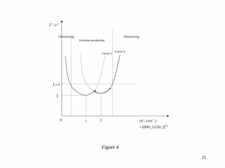
)1/2.

Therefore, we can also obtain the (ecy/cy)-curve as a function of (noy/nox), which is the dashedU-shape curve-1 in Figure 4. If each firm owns two basic products in intermediate-good

production, it is easy to show that the (ecy/cy)-curve will become the dashed U-shape curve-2 inFigure 4. Notice that the minimum point of curve-2 is higher than that of curve-1 as long as

there are management costs of having multiple basic products. Although Figure 4 only draws

these two curves, the same logic applies as the number of the basic products increases.

Then, similar to the relationship between the short-run and long-run cost curves in the

standard production theory, the (ecy/cy)-curve in the presence of multiple basic products is thecontour of these curves, i.e., the solid curve in Figure 4. From a big perspective, this solid

curve is qualitatively the same as the one in Figure 3. Therefore, our main results will still

hold even when firms are allowed to have multiple basic products.

14

5 Concluding Remarks

In this paper we have developed a simple model of two-stage production in which economies-of-

scope play an important role in a vertically-linked production structure. The model allows us to

identify the general patterns of outsourcing and discuss how outsourcing activities are affected

by the degree of product differentiation and economies-of-scope in production. It is also shown

that the main insight of our results are robust even if we relax the key assumption in the model.

Our results on the patterns of outsourcing can be easily formulated as some testable hypotheses,

and we hope they will attract the attention for further empirical investigations.

The paper provides a relatively simple framework that is able to shed some light on wide-

ranging outsourcing activities across industries. In the paper we have considered the case with

only one sector of differentiated products. The model can also be generalized to the case

with multiple sectors of differentiated products. Then, it can be used to explore the impact

of variations across sectors on the relative prevalence of vertically-integrated production vs.

vertically-disintegrated production (outsourcing).

15

References

Antras, Pol 2003, “Firms, contracts, and trade structure”, Quarterly Journal of Economics 118,

1375-1418.

Antras, Pol and Elhanan Helpman 2004, “Global Sourcing”, Journal of Political Economy, 112,

552-580.

Davis, Edward W., “Global outsourcing: Have U.S. managers thrown the baby out with the

bath water?” Business Horizons, July/Aug92, v35(4), pp.58-64.

Eaton, B. Curtis and Schmitt, Nicolas, “Flexible manufacturing and market structure”, Amer-

ican Economic Review 84, September 1994, 875-888.

Grossman, G.M. and Helpman, E., 2002, “Integration vs. outsourcing in industry equilibrium”

Quarterly Journal of Economics 117, pp85-120.

Grossman, Gene and Elhanan Helpman, 2005 “Outsourcing in a global economy”, Review of

Economic Studies, 72, pp135-159.

Feenstra, Robert C. 1998, “Integration of trade and disintegration of production in the global

economy”, Journal of Economic Literature, v12(4), pp31-50.

Feenstra, Robert C. and Gordon H Hanson 2003, “Ownership and control in outsourcing to

China: estimating the property-rights theory of the firm”, NBER Working Paper No. 10198

Hanson, Gordon H. “Localization economics, vertical organization, and trade.” American Eco-

nomic Review 86, 1996, pp1266-78.

MacLeod, W.B., G. Norman and J.-F. Thisse 1988, “Price discrimination and equilibrium in

monopolistic competition”, International Journal of Industrial Organization 6, 429-446.

McLaren, John, 2000, “Globalization and vertical structure.” American Economic Review v90,

1239-1254.

Milgrom, Paul and John Roberts, 1990, “The economics of modern manufacturing: technology,

strategy, and organization”, American Economic Review v80, p511-528.

Milgrom, Paul, Yingyi Qian, and John Roberts, 1991, “Complementarities, mormentum, and

the evolution of modern manufacturing”, American Economic Review Papers and Proceedings,

May 1991, p84-88.

Norman, G. and J.-F. Thisse 1999, “Technology choice and market structure: strategic aspects

of flexible manufacturing”, The Journal of Industrial Economics XLVII, 345-372.

16

Pepall, L., D.J. Richards, and G. Norman, 1999, Industrial Organization: Contemporary Theory

and Practice, Toronto: South-Western College Publishing,

Raff, Daniel M.G., “Making cars and making money in the interwar automobile industry:

economies of scale and scope and the manufacturing behind the marketing”, Business History

Review 65 (Winter 1991), 721-53.

Tirole, Jean, 1988, The Theory of Industrial Organization,The MIT Press, Cambridge, Mass.

Appendix: Figures 1-4 and Table 1.

17

Lθ

L

iX

iY

jx

jy

Figure 1

18

iX

1+iX

xxnL −/

x

Figure 2

iX 1+iX1−iX x

|/|~1 xnLrc x

yi −++ xrc x

yi +~

Indirect Indifference Curves

.A

19

yy cc /~

1

τ+1

2ΩL2ΩU

2

Figure 3

.A C.

In-house production

Outsourcing(ii)

Outsourcing(i)

B.

)//)]/(

)/()(

Krkr

krKr

xy

xy

([θ

=θ

20

yy cc /~

1

τ+1

1 2

In-house productionOutsourcingOutsourcing

5.0)]2/()[()/()(

xy

xo

yo

krKrnn

θ=

Figure 4

0

Curve-1 Curve-2

21

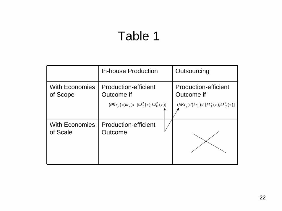
Table 1

In-house Production Outsourcing

With Economies of Scope

Production-efficient Outcome if

Production-efficient Outcome if

With Economies of Scale

Production-efficient Outcome

)](),([)/()( 22 ττθ ULxy krKr ΩΩ∈ )](),([)/()( 22 ττθ ULxy krKr ΩΩ∉

22